Multireference Algebraic Diagrammatic Construction Theory for Excited States: Extended Second-Order Implementation and Benchmark

Abstract

We present an implementation and benchmark of new approximations in multireference algebraic diagrammatic construction theory for simulations of neutral electronic excitations and UV/Vis spectra of strongly correlated molecular systems (MR-ADC). Following our work on the first-order MR-ADC approximation [J. Chem. Phys. 2018, 149, 204113], we report the strict and extended second-order MR-ADC methods (MR-ADC(2) and MR-ADC(2)-X) that combine the description of static and dynamic electron correlation in the ground and excited electronic states without relying on state-averaged reference wavefunctions. We present an extensive benchmark of the new MR-ADC methods for excited states in several small molecules, including the carbon dimer, ethylene, and butadiene. Our results demonstrate that for weakly-correlated electronic states the MR-ADC(2) and MR-ADC(2)-X methods outperform the third-order single-reference ADC approximation and are competitive with the results from equation-of-motion coupled cluster theory. For states with multireference character, the performance of the MR-ADC methods is similar to that of an N-electron valence perturbation theory. In contrast to conventional multireference perturbation theories, the MR-ADC methods have a number of attractive features, such as a straightforward and efficient calculation of excited-state properties and a direct access to excitations outside of the frontier (active) orbitals.

1 Introduction

Ab initio electronic structure methods^{1, 2, 3, 4} are often used in combination with experiment to gain a deeper understanding of the excited-state properties of molecules and to study the behavior of these molecules as they undergo various photochemical transformations. Among many quantum chemical methods, algebraic diagrammatic construction theory^{5, 6, 7, 8, 9} (ADC) has become one of the widely used approaches for studying electronically excited states,^{10, 11, 12, 13, 14, 15, 16, 17, 18, 19, 20, 21, 22, 23, 24, 25} due to a combination of its low computational cost and systematically improvable accuracy. In its original formulation proposed almost 40 years ago,⁵ ADC is based on the conventional (single-reference) perturbation theory, which significantly simplifies its working equations and allows for efficient calculation of excitation energies and excited-state properties. However, due to its single-reference nature, conventional ADC approximations become unreliable in systems with strong electron correlation in the ground or excited electronic states.

Recently, we proposed a multireference formulation of ADC²⁶ (MR-ADC) that can be considered as a natural generalization of the conventional ADC theory for strongly-correlated (multiconfigurational) wavefunctions. MR-ADC combines the advantages of the multireference perturbation theories,^{27, 28, 29, 30, 31, 32, 33, 34, 35, 36, 37, 38, 39, 40, 41, 42} effective Hamiltonian approaches,^{43, 44, 45, 46, 47, 48, 49, 50, 51} and multiconfigurational propagator methods^{52, 53, 54, 55, 56, 57, 58, 59, 60, 61} in a single theoretical framework that offers a hierarchy of computationally efficient approximations that provide a straightforward access to size-consistent excitation energies and excited-state properties and allow for calculation of excitations outside of strongly-correlated (active) orbitals. More recent work in our group concentrated on the development of the second-order MR-ADC approximations for simulating charged excitations (such as electron attachment or ionization) and demonstrated that the MR-ADC methods perform very well in a variety of weakly- and strongly-correlated systems.^{62, 63} On the other hand, our computer implementation of MR-ADC for neutral electronic excitations has been limited to the first-order MR-ADC approximation (MR-ADC(1)),²⁶ which did not provide accurate excitation energies missing much of the dynamic correlation effects.

In this work, we present the implementation and benchmark of the strict and extended second-order MR-ADC methods (MR-ADC(2) and MR-ADC(2)-X) for neutral electronic excitations that provide a more balanced description of static and dynamic electron correlation effects. We present an overview of the MR-ADC theory for neutral excitations in Section 2, before outlining the principle components of our implementation in Section 3. We lay out the details of our computations in Section 4 and present our benchmark results for excited states of small molecules (HF, CO, N2, F2, H2O), the carbon dimer (C2), as well as the ethylene (C2H4) and butdiene (C4H6) molecules in Section 5. Our results demonstrate that the second-order MR-ADC approximations provide accurate predictions of the excited-state energies for weakly- and strongly-correlated electronic states at equilibrium geometries and near dissociation. We outline our conclusions in Section 6.

2 Theory

2.1 MR-ADC for the Polarization Propagator

We begin with a brief overview of the principal components of the MR-ADC theory in the context of neutral (particle-number-conserving) electronic excitations. A more detailed discussion of MR-ADC using the formalism of the effective Liouvillean theory⁶⁴ can be found in Ref. 26. Electronic excitations arise from the perturbation of a molecule by an external electric field. The response of the molecule is described by the spectral function⁵

$$T(\omega)=-\frac{1}{\pi}\operatorname{Tr}\left[\operatorname{Im}(\mathbf{D^{{\dagger}}}\mathbf{\Pi}(\omega)\mathbf{D})\right]$$ (1)

where $\mathbf{D}$ is a dipole moment operator matrix with elements $D_{pq}$ expressed in a finite single-particle basis set and $\mathbf{\Pi}(\omega)$ is a polarization propagator, which is the central object of interest in this work.

The polarization propagator $\mathbf{\Pi}(\omega)$ is a particular type of the retarded frequency-dependent propagator^{3, 4} $\mathbf{G}(\omega)$, which can be generally written as:

$$G_{\mu\nu}(\omega) =G_{\mu\nu}^{+}(\omega)\pm G_{\mu\nu}^{-}(\omega)$$

$$=\bra{\Psi}q_{\mu}(\omega-H+E)^{-1}q^{\dagger}_{\nu}\ket{\Psi}$$

$$\pm\bra{\Psi}q^{\dagger}_{\nu}(\omega+H-E)^{-1}q_{\mu}\ket{\Psi}$$ (2)

where $G_{\mu\nu}^{+}(\omega)$ and $G_{\mu\nu}^{-}(\omega)$ are the forward and backward components of the propagator, $H$ is the electronic Hamiltonian, $\ket{\Psi}$ and $E$ are the eigenfunction and eigenenergy of $H$, respectively. The polarization propagator $\mathbf{\Pi}(\omega)$ is characterized by the choice of $q^{\dagger}_{\nu}=a^{\dagger}_{p}a_{q}-\bra{\Psi}a^{\dagger}_{p}a_{q}\ket{\Psi}$, expressed in terms of the fermionic annihilation and creation operators, and the negative sign for the second term in Section 2.1. In the case of the polarization propagator, the forward and backward components are related as $\mathbf{\Pi}_{+}^{\dagger}(-\omega)=-\mathbf{\Pi}_{-}(\omega)$, so in computing one component, the other is trivially obtained. For this reason, in this work we define $\mathbf{\Pi}(\omega)\equiv\mathbf{\Pi}_{+}(\omega)$ and consider only the forward component of the propagator henceforth.

When written in the equivalent Lehmann⁶⁵ (spectral) representation, in which a resolution of identity is introduced over all excited eigenstates of the system ($\ket{\Psi_{k}}$),

$$\Pi_{pqrs}(\omega)=\sum_{k\neq 0}\frac{\braket{\Psi}{a^{\dagger}_{q}a_{p}}{\Psi_{k}}\braket{\Psi_{k}}{a^{\dagger}_{r}a_{s}}{\Psi}}{\omega+E_{0}-E_{k}}.$$ (3)

the poles of the polarization propagator $\Pi_{pqrs}(\omega)$ correspond to excitation energies ($\omega_{k}=E_{k}-E_{0}$) while the expectation values in the numerator describe the probabilities of the corresponding transitions. The frequency $\omega\equiv\omega^{\prime}+i\eta$ is defined in terms of real ($\omega^{\prime}$) and infinitesimal imaginary ($i\eta$) components. Eq. 3 can be written compactly in a matrix form

$$\mathbf{\Pi}(\omega)=\mathbf{\tilde{X}}(\omega-\mathbf{\tilde{\Omega}})^{-1}\mathbf{\tilde{X}}^{\dagger}$$ (4)

where $\mathbf{\tilde{\Omega}}$ is a diagonal matrix of excitation energies ($\omega_{k}$) and $\mathbf{\tilde{X}}$ is a matrix of spectroscopic amplitudes $\tilde{X}_{pqk}=\braket{\Psi}{a^{\dagger}_{q}a_{p}}{\Psi_{k}}$. The expressions for the polarization propagator in Eqs. 3 and 4 are exact if written in the basis of the exact eigenstates, however in practice these states must be approximated.

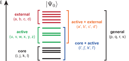
Figure 1: Orbital indexing convention used in this work.

MR-ADC provides a hierarchy of efficient approximations to the polarization propagator (4) by expressing it in a time-independent multireference perturbative expansion and truncating this series at a low order in perturbation theory. Working equations of the MR-ADC approximations are derived using the multireference generalization of the effective Liouvillean theory^{26, 64}, which starts by writing the wavefunction $\ket{\Psi}$ as a unitary transformation^{66, 67, 64, 68, 69, 70} of the complete active-space self-consistent field⁷¹ (CASSCF) reference wavefunction $\ket{\Psi_{0}}$

$$\ket{\Psi} =e^{A}\ket{\Psi_{0}}=e^{T-T^{\dagger}}\ket{\Psi_{0}},\quad T=\sum_{k=1}^{N}T_{k}$$ (5)

$$T_{k} =\frac{1}{(k!)^{2}}{\sum_{i^{\prime}j^{\prime}a^{\prime}b^{\prime}\ldots}}t_{i^{\prime}j^{\prime}\ldots}^{a^{\prime}b^{\prime}\ldots}a^{\dagger}_{a^{\prime}}a^{\dagger}_{b^{\prime}}\ldots a_{j^{\prime}}a_{i^{\prime}}$$ (6)

In Eqs. 5 and 6, $T$ is an excitation operator that generates all of the internally-contracted excitations between the core, active, and external orbitals (Figure 1). Next, the full electronic Hamiltonian $H$ is partitioned into the zeroth-order part $H^{(0)}$ and a perturbation $V=H-H^{(0)}$, where $H^{(0)}$ is the Dyall Hamiltonian^{72, 33, 34, 35} with an eigenfunction $\ket{\Psi_{0}}$. This partitioning of $H$ leads to the perturbative expansions for the wavefunction $\ket{\Psi}$ and the polarization propagator $\mathbf{\Pi}(\omega)$:

$$\ket{\Psi} =e^{A^{(0)}+A^{(1)}+\cdots+A^{(n)}+\cdots}\ket{\Psi_{0}}$$ (7)

$$\mathbf{\Pi}(\omega) =\mathbf{\Pi}^{(0)}(\omega)+\mathbf{\Pi}^{(1)}(\omega)+\cdots+\mathbf{\Pi}^{(n)}(\omega)+\cdots$$ (8)

Truncating these expansions at the n^th order defines the polarization propagator of the MR-ADC(n) approximation. The MR-ADC(n) working equations are derived by writing $\mathbf{\Pi}(\omega)$ in the form

$$\mathbf{\Pi}(\omega)=\mathbf{T}(\omega\mathbf{S}-\mathbf{M})^{-1}\mathbf{T}^{{\dagger}}$$ (9)

where $\mathbf{M}$ is a non-diagonal effective Hamiltonian matrix that can be used to compute the excitation energies and $\mathbf{T}$ is an effective transition moments matrix that contains information about the probabilities of electronic transitions. The matrices $\mathbf{M}$ and $\mathbf{T}$ are evaluated in an approximate basis of many-electron (internally-contracted) states, which are in general non-orthogonal with an overlap matrix $\mathbf{S}$. In Eq. 9 each matrix is evaluated up to the same (n^th) order in perturbation theory.

The MR-ADC(n) excitation energies $\mathbf{\Omega}$ and complementary eigenvectors $\mathbf{Y}$ are obtained by solving the generalized eigenvalue problem

$$\mathbf{M}\mathbf{Y}=\mathbf{S}\mathbf{Y}\mathbf{\Omega}$$ (10)

Combining the eigenvectors $\mathbf{Y}$ with the effective transition moments matrix $\mathbf{T}$ allows to compute the spectroscopic amplitudes

$$\mathbf{X}=\mathbf{T}\mathbf{S}^{-\frac{1}{2}}\mathbf{Y}$$ (11)

and the MR-ADC(n) polarization propagator

$$\mathbf{\Pi}(\omega)=\mathbf{X}(\omega-\mathbf{\Omega})^{-1}\mathbf{X}^{\dagger}$$ (12)

along with the spectral function $T(\omega)$ in Eq. 1. The spectroscopic amplitudes $\mathbf{X}$ can be also used to compute the oscillator strength for each electronic transition $k$

$$f_{k}=\frac{2}{3}\omega_{k}\left|\braket{\Psi}{D}{\Psi_{k}}\right|^{2}=\frac{2}{3}\omega_{k}\left(\sum_{pq}D_{pq}X_{pqk}\right)^{2}$$ (13)

where $\braket{\Psi}{D}{\Psi_{k}}$ is the transition dipole moment matrix element.

2.2 Strict and Extended Second-Order MR-ADC Approximations

2.2.1 Perturbative Structure of the MR-ADC Matrices

In this work, we consider the strict and extended second-order MR-ADC approximations for electronic excitations, denoted as MR-ADC(2) and MR-ADC(2)-X. In the MR-ADC(2) approximation, contributions to $\mathbf{\Pi}(\omega)$ are included strictly up to the second order in the MR-ADC perturbation expansion, while the MR-ADC(2)-X method partially incorporates selected third-order terms as discussed below.

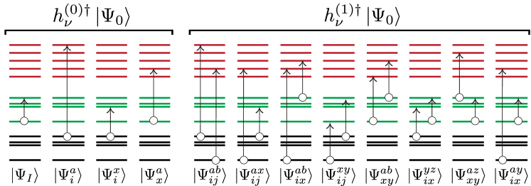
Figure 2: Schematic illustration of the electronically-excited basis states produced by acting the $h_{\nu}^{(k){\dagger}}$ ($k=0,1$) operators (Eqs. 17 and 18) on the reference state $\ket{\Psi_{0}}$. A circle connected with an arrow denotes a single excitation. Black, green, and red lines represent core, active, and external orbitals, respectively.

At each perturbation order n, contributions to the matrix elements of $\mathbf{M}$, $\mathbf{T}$, and $\mathbf{S}$ in Eq. 9 are expressed as

$$M^{(n)}_{\mu\nu} =\sum^{k+l+m=n}_{klm}\braket{\Psi_{0}}{[h^{(k)}_{\mu},[\tilde{H}^{(l)},h^{(m){\dagger}}_{\nu}]]}{\Psi_{0}}$$ (14)

$$T^{(n)}_{\mu\nu} =\sum^{k+m=n}_{km}\braket{\Psi_{0}}{[\tilde{q}^{(k)}_{\mu},h^{(m){\dagger}}_{\nu}]}{\Psi_{0}}$$ (15)

$$S^{(n)}_{\mu\nu} =\sum^{k+m=n}_{km}\braket{\Psi_{0}}{[h^{(k)}_{\mu},h^{(m){\dagger}}_{\nu}]}{\Psi_{0}}$$ (16)

where $\tilde{H}^{(l)}$ and $\tilde{q}^{(l)}_{\mu}$ are the $\mathit{l}$^th-order operators obtained from the perturbative analysis of the Baker–Campbell–Hausdorff expansions for the effective Hamiltonian $\tilde{H}=e^{-A}He^{A}$ and observable $\tilde{q}_{\mu}=e^{-A}q_{\mu}e^{A}$ operators, respectively. The excitation operators $h^{(m){\dagger}}_{\nu}$ are used to construct the many-electron basis states that are necessary for representing the wavefunctions of the excited electronic states. Defining $a^{p}_{q}\equiv a^{\dagger}_{p}a_{q}$ and $a^{pq}_{rs}\equiv a^{\dagger}_{p}a^{\dagger}_{q}a_{s}a_{r}$, the low-order $h^{(m){\dagger}}_{\nu}$ used in MR-ADC(2) and MR-ADC(2)-X have the form:

$$\mathbf{h}^{(0){\dagger}} =\{Z^{\dagger}_{I}\ (I>0),\ a^{a}_{i},\ a^{x}_{i},\ a^{a}_{x}\}$$ (17)

$$\mathbf{h}^{(1){\dagger}} =\{a^{ab}_{ij},\ a^{ax}_{ij},\ a^{ab}_{ix},\ a^{xy}_{ij},\ a^{ab}_{xy},\ a^{yz}_{ix},\ a^{az}_{xy},\ a^{ay}_{ix}\}$$ (18)

These excitations are pictorially represented in Figure 2. The $\mathbf{h}^{(0){\dagger}}$ operator set contains two classes of operators: (i) the eigenoperators^{73, 74} $Z^{\dagger}_{I}=\ket{\Psi_{I}}\bra{\Psi_{0}}$ $(I>0)$ that describe excitations within the active space and (ii) the operators $a^{p}_{q}$ that produce single excitations outside of the active space. The excited-state active-space wavefunctions $\ket{\Psi_{I}}$ $(I>0)$ that appear in $Z^{\dagger}_{I}$ are obtained by performing a multistate CASCI calculation using the CASSCF orbitals optimized for the reference state $\ket{\Psi_{0}}$. Although, formally, the set of $\ket{\Psi_{I}}$ $(I>0)$ includes all CASCI wavefunctions in a given complete active space, in practice only a small number of CASCI states relevant to the spectral region of interest need to be computed. As shown in Figure 2, the $\mathbf{h}^{(1){\dagger}}$ operator set describes all possible double excitations outside of the active space.

Eqs. 14 and 15 define the perturbative structure of the $\mathbf{M}$ and $\mathbf{T}$ matrices shown in Figure 3, with the effective operators $\tilde{H}^{(k)}$ and $\tilde{q}^{(l)}$ expanded to different orders in different sectors defined by the $h^{(0){\dagger}}_{\nu}$ and $h^{(1){\dagger}}_{\nu}$ operators. Both MR-ADC(2) and MR-ADC(2)-X incorporate up to $\tilde{H}^{(2)}$ in the $\braket{\Psi_{0}}{[h^{(0)}_{\mu},[\tilde{H}^{(l)},h^{(0){\dagger}}_{\nu}]]}{\Psi_{0}}$ sector of the $\mathbf{M}$ matrix and up to $\tilde{H}^{(1)}$ in the $h^{(0)}_{\mu}$ – $h^{(1){\dagger}}_{\nu}$ and $h^{(1)}_{\mu}$ – $h^{(0){\dagger}}_{\nu}$ coupling blocks. The two methods differ in the $h^{(1)}_{\mu}$ – $h^{(1){\dagger}}_{\nu}$ sector approximating the effective Hamiltonian to $\tilde{H}^{(0)}$ and $\tilde{H}^{(1)}$ in MR-ADC(2) and MR-ADC(2)-X, respectively. For the $\mathbf{T}$ matrix, MR-ADC(2) and MR-ADC(2)-X describe the effective observable operator up to $\tilde{q}^{(2)}$ in the $h^{(0){\dagger}}_{\nu}$ sector, but differ in its expansion in the $h^{(1){\dagger}}_{\nu}$ block (Figure 3). We note that the perturbative structure of the $\mathbf{M}$ and $\mathbf{T}$ matrices in MR-ADC is very similar to that in single-reference ADC⁹ and the two theories become equivalent when the number of active orbitals is zero.

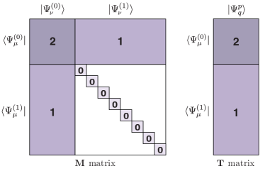
(a)

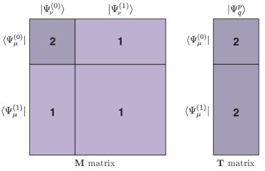
(b)

Figure 3: Graphical representation of the effective Hamiltonian $\mathbf{M}$ and transition moments $\mathbf{T}$ matrices for the a) MR-ADC(2) and b) MR-ADC(2)-X methods.

2.2.2 Amplitudes of the Effective Hamiltonian

Computation of the $\mathbf{M}$ and $\mathbf{T}$ matrix elements in Figure 3 requires solving for the amplitudes of the excitation operator $T^{(k)}$ (Eq. 6). We express $T^{(k)}$ in a general form as

$$T^{(k)}=\mathbf{t^{(k)}}\,\boldsymbol{\tau}^{\dagger}=\sum_{\mu}t_{\mu}^{(k)}\tau^{\dagger}_{\mu}$$ (19)

where $t_{\mu}^{(k)}$ are the kth-order amplitude coefficients and $\tau^{\dagger}_{\mu}$ denotes the corresponding string of creation and annihilation operators. In MR-ADC(2) and MR-ADC(2)-X only the low-order amplitudes $\mathbf{t^{(1)}}$ and $\mathbf{t^{(2)}}$ need to be evaluated. These amplitudes are determined by solving a system of projected linear equations

$$\braket{\Psi_{0}}{\tau_{\mu}\tilde{H}^{(k)}}{\Psi_{0}}=0\qquad(k=1,\ 2)$$ (20)

For the details of solving these amplitude equations we refer the readers to our earlier publications.^{62, 63}

Both MR-ADC(2) and MR-ADC(2)-X require calculating all first-order amplitudes, specifically:

$$\mathbf{t^{(1)}}= \left\{t_{i}^{a(1)};\ t_{i}^{x(1)};\ t_{x}^{a(1)};\ t_{ij}^{ab(1)};\ t_{ij}^{ax(1)};\ t_{ix}^{ab(1)};\right.$$

$$\left.t_{ij}^{xy(1)};\ t_{xy}^{ab(1)};\ t_{ix}^{ay(1)};\ t_{ix}^{yz(1)};\ t_{xy}^{az(1)}\right\}$$ (21)

The first three sets of amplitudes correspond to single excitations ($t_{i}^{a(1)};\ t_{i}^{x(1)};\ t_{x}^{a(1)}$) and the next five sets represent external double excitations. The last three sets of $\mathbf{t^{(1)}}$ in Section 2.2.2 describe the semi-internal double excitations ($t_{ix}^{ay(1)};\ t_{ix}^{yz(1)};\ t_{xy}^{az(1)}$).

The MR-ADC(2) and MR-ADC(2)-X equations for the effective Hamiltonian matrix $\mathbf{M}$ also depend on the second-order singles and semi-internal doubles amplitudes of the form:

$$\mathbf{t^{(2)}_{s}}= \left\{t_{i}^{a(2)};\ t_{i}^{x(2)};\ t_{x}^{a(2)};\ t_{x}^{y(2)}(x>y);\right.$$

$$\left.t_{ix}^{ay(2)};\ t_{ix}^{yz(2)};\ t_{xy}^{az(2)}\right\}$$ (22)

We note that in addition to the external singles amplitudes ($t_{i}^{a(2)};\ t_{i}^{x(2)};\ t_{x}^{a(2)}$), Section 2.2.2 also includes the internal singles amplitudes $t_{x}^{y(2)}(x>y)$ that we did not encounter in our previous work. These amplitudes are necessary to ensure the Hermiticity of the effective Hamiltonian matrix $\mathbf{M}$ as discussed below. Additionally, the MR-ADC(2)-X equations for the $\mathbf{T}$ matrix elements (Figure 3b) depend on the external double-excitation amplitudes

$$\mathbf{t^{(2)}_{d}}= \left\{t_{ij}^{ab(2)};\ t_{ij}^{ax(2)};t_{ix}^{ab(2)};\ t_{ij}^{xy(2)};\ t_{xy}^{ab(2)}\right\}$$ (23)

In our previous work on EA/IP-MR-ADC(2) and EA/IP-MR-ADC(2)-X,^{62, 63} we demonstrated that neglecting all second-order amplitudes except $t_{i}^{a(2)}$ has a negligible effect on the computed charged excitation energies and transition probabilities. However, for neutral electronic excitations, some of the second-order amplitudes need to be computed to prevent asymmetry of the $\mathbf{M}$ matrix. To illustrate this, we consider the second-order contributions to one of the off-diagonal blocks of $\mathbf{M}$ and its transpose that can be expressed and simplified as:

$$M^{(2)}_{ix,jb}= \braket{\Psi_{0}}{[a^{\dagger}_{i}a_{x},[\tilde{H}^{(2)},a^{\dagger}_{b}a_{j}]]}{\Psi_{0}}$$

$$= \braket{\Psi_{0}}{a^{\dagger}_{i}a_{x}\tilde{H}^{(2)}a^{\dagger}_{b}a_{j}}{\Psi_{0}}$$ (24)

$$M^{(2){\dagger}}_{ix,jb}= \braket{\Psi_{0}}{[a^{\dagger}_{j}a_{b},[\tilde{H}^{(2)},a^{\dagger}_{x}a_{i}]]}{\Psi_{0}}^{\dagger}$$

$$= \braket{\Psi_{0}}{a^{\dagger}_{i}a_{x}\tilde{H}^{(2)}a^{\dagger}_{b}a_{j}}{\Psi_{0}}$$

$$+ \delta_{{i}}^{{j}}\braket{\Psi_{0}}{\tilde{H}^{(2)}a^{\dagger}_{b}a_{x}}{\Psi_{0}}$$ (25)

The two blocks of the $\mathbf{M}$ matrix are equal to each other provided that the second term in Section 2.2.2 is zero, which is satisfied if the second-order effective Hamiltonian $\tilde{H}^{(2)}$ is parametrized with the $t_{x}^{b(2)}$ amplitudes that fulfill the projected amplitude equations $\braket{\Psi_{0}}{\tilde{H}^{(2)}a^{\dagger}_{b}a_{x}}{\Psi_{0}}=0$ (Eq. 20). As another example we consider one of the diagonal blocks of $\mathbf{M}$:

$$M^{(2)}_{ix,jy}= \braket{\Psi_{0}}{[a^{\dagger}_{i}a_{x},[\tilde{H}^{(2)},a^{\dagger}_{y}a_{j}]]}{\Psi_{0}}$$

$$= \braket{\Psi_{0}}{a^{\dagger}_{i}a_{x}\tilde{H}^{(2)}a^{\dagger}_{y}a_{j}}{\Psi_{0}}$$

$$- \delta_{{i}}^{{j}}\braket{\Psi_{0}}{a_{x}a^{\dagger}_{y}\tilde{H}^{(2)}}{\Psi_{0}}$$ (26)

$$M^{(2){\dagger}}_{ix,jy}= \braket{\Psi_{0}}{[a^{\dagger}_{j}a_{y},[\tilde{H}^{(2)},a^{\dagger}_{x}a_{i}]]}{\Psi_{0}}^{\dagger}$$

$$= \braket{\Psi_{0}}{a^{\dagger}_{i}a_{x}\tilde{H}^{(2)}a^{\dagger}_{y}a_{j}}{\Psi_{0}}$$

$$- \delta_{{i}}^{{j}}\braket{\Psi_{0}}{\tilde{H}^{(2)}a_{x}a^{\dagger}_{y}}{\Psi_{0}}$$ (27)

Here, the last two terms in Sections 2.2.2 and 2.2.2 are in general different, unless the effective Hamiltonian includes contributions from the internal second-order amplitudes $t_{x}^{y(2)}(x>y)$ ensuring that $\braket{\Psi_{0}}{a_{x}a^{\dagger}_{y}\tilde{H}^{(2)}}{\Psi_{0}}=\braket{\Psi_{0}}{\tilde{H}^{(2)}a_{x}a^{\dagger}_{y}}{\Psi_{0}}$, which results in the Hermitian $M^{(2)}_{ix,jy}$ block. The solution of the amplitude equations for the $t_{x}^{y(2)}(x>y)$ amplitudes is described in the Appendix.

Including all second-order singles amplitudes ensures the full Hermiticity of the $\mathbf{M}$ matrix in all sectors. On the other hand, neglecting the second-order doubles amplitudes does not affect the symmetry of $\mathbf{M}$ and has a negligible effect on the computed excitation energies and oscillator strengths (see Table S1 of the Supporting Information for details). For this reason, in our implementation of MR-ADC for electronic excitations, we approximate:

$$\mathbf{t^{(2)}}\approx \left\{t_{i}^{a(2)};\ t_{i}^{x(2)};\ t_{x}^{a(2)};\ t_{x}^{y(2)}(x>y)\right\}$$ (28)

3 Implementation

Our implementation of MR-ADC(2) and MR-ADC(2)-X for electronic excitations follows the steps outlined below:

1. Given an active space, compute the reference (usually, ground-state) CASSCF wavefunction $\ket{\Psi_{0}}$ and molecular orbitals.

2. Using the reference CASSCF molecular orbitals compute the CASCI wavefunctions $\ket{\Psi_{I}}\,(I>0)$ for the user-defined number of excited states ($N_{\mathrm{CI}}$).

3. Calculate the reduced density matrices (RDMs):

   1. reference RDMs with respect to $\ket{\Psi_{0}}$;

   2. transition RDMs between $\ket{\Psi_{0}}$ and $\ket{\Psi_{I}}\,(I>0)$;

   3. excited-state RDMs amongst $\ket{\Psi_{I}}\,(I>0)$.

4. Solve the linear amplitude equations (Eq. 20) to compute the first- and second-order amplitudes $\mathbf{t^{(1)}}$ and $\mathbf{t^{(2)}}$ discussed in Section 2.2.2.

5. Diagonalize the effective Hamiltonian matrix $\mathbf{M}$ (Eq. 10) to compute excitation energies.

6. Compute the spectroscopic amplitudes $\mathbf{X}$ (Eq. 11) and oscillator strengths $f_{k}$ (Eq. 13).

As discussed in our previous work,^{62, 63} the MR-ADC generalized eigenvalue problem is solved in the symmetrically-orthogonalized form ($\mathbf{\tilde{M}}\,\mathbf{\tilde{Y}}=\mathbf{\tilde{Y}}\,\mathbf{\Omega}$, $\mathbf{\tilde{M}}=\mathbf{S^{-1/2}}\,\mathbf{M}\,\mathbf{S^{-1/2}}$, $\mathbf{\tilde{Y}}=\mathbf{S^{1/2}}\,\mathbf{Y}$) using the multiroot Davidson algorithm^{75, 76} that iteratively optimizes the eigenvectors $\mathbf{\tilde{Y}}$ until convergence by forming the matrix-vector products $\boldsymbol{\sigma}=\mathbf{\tilde{M}\tilde{Y}}$. We note that the $\mathbf{S^{-1/2}}$ matrix has a block-diagonal structure that allows to avoid storing the full matrix in memory. The small non-diagonal blocks of $\mathbf{S^{-1/2}}$ are computed very efficiently by diagonalizing small sectors of the overlap matrix $\mathbf{S}$.⁶² Equations and computer code for the calculation of the $\boldsymbol{\sigma}$ vectors were generated using a modified version of the SecondQuantizationAlgebra program (SQA) developed by Neuscamman and co-workers.⁷⁷ To optimize computational efficiency, our code generator implements the tensor contractions by automatically separating them into the efficient tensor intermediates, which are reused throughout the calculation.

For a fixed active space, the MR-ADC(2) and MR-ADC(2)-X implementations have the $\mathcal{O}(M^{5})$ and $\mathcal{O}(M^{6})$ computational scaling with the basis set size $M$, respectively, which is equivalent to the scaling of their single-reference counterparts.⁹ Both methods have the formal $\mathcal{O}(N_{\mathrm{det}}N^{8}_{\mathrm{act}})$ scaling with the number of active orbitals ($N_{\mathrm{act}}$) and Slater determinants ($N_{\mathrm{det}}$), similar to that of the conventional second-order multireference perturbation theories. The active-space scaling can be further lowered to $\mathcal{O}(N_{\mathrm{det}}N^{6}_{\mathrm{act}})$ using a technique described in our previous work,^{62, 63} which forms efficient intermediates to avoid computation of the four-particle RDMs, although we did not employ this approach in our current implementation.

4 Computational Details

The MR-ADC(2) and MR-ADC(2)-X methods were implemented in Prism, a standalone program that is being developed in our group. The Prism program interfaces with PySCF⁷⁸ to obtain integrals and CASSCF/CASCI reference wavefunctions. The MR-ADC results were benchmarked against excitation energies obtained from the semi-stochastic heat-bath configuration interaction (SHCI)^{79, 80, 81} calculations extrapolated to the full configuration interaction limit. The SHCI method was implemented in the Dice program.^{79, 80, 81} We also compare the MR-ADC results to those computed using strongly-contracted $N$-electron valence second-order perturbation theory (sc-NEVPT2),^{33, 34} single-reference ADC (ADC(n), n = 2, 3),^{5, 9} and equation-of-motion coupled cluster theory with single and double excitations (EOM-CCSD)^{82, 83, 84, 85}. We used PySCF to obtain the sc-NEVPT2 energies. The ADC(2), ADC(3), and EOM-CCSD results were computed using Q-Chem⁸⁶.

Performance of the MR-ADC(2) and MR-ADC(2)-X methods was tested for a benchmark set of five small molecules (HF, F2, CO, N2, and H2O), a carbon dimer (C2), and two alkenes: ethylene and butadiene. As in our earlier work,^{62, 63} computations of the five small molecules were performed using two geometries: equilibrium and stretched. The equilibrium geometries were taken from Ref. 13. The stretched geometries of all molecules were obtained by increasing their bond lengths by a factor of two. The C$-$C bond distance in the carbon dimer was set to 2.4 $a_{0}$, which is close to its equilibrium bond length.⁸⁷ The geometries of the alkenes were obtained as described in Ref. 88 and are reported in the Supporting Information. Calculations of HF, F2, CO, N2, and H2O employed the aug-cc-pVDZ basis set.⁸⁹ Carbon dimer calculations were performed using cc-pVDZ.⁹⁰ For the ethylene and butadiene molecules we used the ANO-L-PVTZ and ANO-L-PVDZ basis sets, respectively.⁹¹

Table 1: Vertical excitation energies ($\Omega$, eV) and oscillator strengths ($f$) of molecules with equilibrium geometries. See Section 4 for details of the calculations. Also shown are mean absolute errors ($\Delta_{\mathrm{MAE}}$), standard deviations ($\Delta_{\mathrm{STD}}$), and maximum absolute errors ($\Delta_{\mathrm{MAX}}$) of the energies, relative to SHCI. Only orbitals participating in excitations are listed in the electron configuration of each excited state.

System	Configuration	Term	ADC(2)	ADC(3)	EOM-CCSD	sc-NEVPT2	MR-ADC(2)	MR-ADC(2)-X	SHCI
			$\Omega\ (f)$	$\Omega\ (f)$	$\Omega$	$\Omega$	$\Omega\ (f)$	$\Omega\ (f)$	$\Omega$
HF	$(3\sigma)^{2}(1\pi)^{3}(4\sigma)^{1}$	${}^{3}\Pi$	$9.30$	$10.50$	$9.89$	$10.09$	$10.40$	$10.21$	$10.05$
	$(3\sigma)^{2}(1\pi)^{3}(4\sigma)^{1}$	${}^{1}\Pi$	$9.63$ ($0.039$)	$10.96$ ($0.042$)	$10.30$	$10.46$	$10.80$ ($0.036$)	$10.58$ ($0.035$)	$10.44$
	$(3\sigma)^{1}(1\pi)^{4}(4\sigma)^{1}$	${}^{3}\Sigma^{+}$	$13.05$	$13.80$	$13.41$	$13.60$	$13.91$	$13.67$	$13.54$
	$(3\sigma)^{2}(1\pi)^{3}(5\sigma)^{1}$	${}^{3}\Pi$	$13.14$	$14.53$	$13.86$	$14.06$	$14.17$	$13.96$	$14.02$
	$(3\sigma)^{2}(1\pi)^{3}(5\sigma)^{1}$	${}^{1}\Pi$	$13.35$ ($0.006$)	$14.74$ ($0.019$)	$14.06$	$14.27$	$14.38$ ($0.010$)	$14.17$ ($0.009$)	$14.21$
	$(3\sigma)^{2}(1\pi)^{3}(2\pi)^{1}$	${}^{3}\Sigma^{+}$	$13.80$	$14.83$	$14.26$	$14.52$	$14.70$	$14.52$	$14.47$
	$(3\sigma)^{1}(1\pi)^{4}(4\sigma)^{1}$	${}^{1}\Sigma^{+}$	$13.91$ ($0.149$)	$15.01$ ($0.178$)	$14.47$	$14.66$	$15.08$ ($0.172$)	$14.77$ ($0.167$)	$14.58$
	$(3\sigma)^{2}(1\pi)^{3}(2\pi)^{1}$	${}^{3}\Delta$	$14.22$	$15.33$	$14.74$	$14.93$	$15.18$	$14.99$	$14.93$
	$(3\sigma)^{2}(1\pi)^{3}(2\pi)^{1}$	${}^{1}\Delta$	$14.46$	$15.66$	$15.03$	$15.20$	$15.49$	$15.29$	$15.20$
	$(3\sigma)^{2}(1\pi)^{3}(2\pi)^{1}$	${}^{3}\Sigma^{-}$	$14.51$	$15.69$	$15.07$	$15.26$	$15.53$	$15.31$	$15.25$
	$(3\sigma)^{1}(1\pi)^{3}(2\pi)^{1}$	${}^{1}\Sigma^{-}$	$14.54$	$15.72$	$15.10$	$15.28$	$15.56$	$15.36$	$15.28$
CO	$(1\pi)^{4}(5\sigma)^{1}(2\pi)^{1}$	${}^{3}\Pi$	$6.49$	$6.00$	$6.42$	$6.57$	$6.51$	$6.02$	$6.33$
	$(1\pi)^{3}(5\sigma)^{2}(2\pi)^{1}$	${}^{3}\Sigma^{+}$	$8.60$	$8.38$	$8.44$	$8.67$	$8.94$	$8.81$	$8.54$
	$(1\pi)^{4}(5\sigma)^{1}(2\pi)^{1}$	${}^{1}\Pi$	$8.82$ ($0.072$)	$8.36$ ($0.093$)	$8.72$	$9.55$	$9.03$ ($0.140$)	$8.42$ ($0.134$)	$8.60$
	$(1\pi)^{3}(5\sigma)^{2}(2\pi)^{1}$	${}^{3}\Delta$	$9.46$	$9.27$	$9.40$	$9.57$	$9.84$	$9.71$	$9.44$
	$(1\pi)^{3}(5\sigma)^{2}(2\pi)^{1}$	${}^{3}\Sigma^{-}$	$10.15$	$9.77$	$9.98$	$10.16$	$10.47$	$9.68$	$9.95$
	$(1\pi)^{3}(5\sigma)^{2}(2\pi)^{1}$	${}^{1}\Sigma^{-}$	$10.21$	$10.02$	$10.21$	$10.32$	$10.58$	$10.43$	$10.17$
	$(1\pi)^{3}(5\sigma)^{2}(2\pi)^{1}$	${}^{1}\Delta$	$10.47$	$10.10$	$10.32$	$10.52$	$10.89$	$10.71$	$10.28$
N2	$(3\sigma_{g})^{2}(1\pi_{u})^{3}(1\pi_{g})^{1}$	${}^{3}\Sigma_{u}^{+}$	$8.20$	$7.36$	$7.74$	$7.86$	$7.93$	$7.86$	$7.74$
	$(3\sigma_{g})^{1}(1\pi_{u})^{4}(1\pi_{g})^{1}$	${}^{3}\Pi_{g}$	$8.25$	$7.85$	$8.15$	$8.14$	$8.82$	$8.38$	$8.09$
	$(3\sigma_{g})^{1}(1\pi_{u})^{4}(1\pi_{g})^{1}$	${}^{3}\Delta_{u}$	$9.37$	$8.57$	$9.09$	$9.12$	$9.17$	$9.08$	$9.03$
	$(3\sigma_{g})^{1}(1\pi_{u})^{4}(1\pi_{g})^{1}$	${}^{1}\Pi_{g}$	$9.60$	$9.32$	$9.53$	$9.41$	$10.04$	$9.59$	$9.45$
	$(3\sigma_{g})^{2}(1\pi_{u})^{3}(1\pi_{g})^{1}$	${}^{3}\Sigma_{u}^{-}$	$10.36$	$9.36$	$10.00$	$10.16$	$10.29$	$10.14$	$9.82$
	$(3\sigma_{g})^{2}(1\pi_{u})^{3}(1\pi_{g})^{1}$	${}^{1}\Sigma_{u}^{-}$	$10.43$	$9.62$	$10.25$	$10.22$	$10.23$	$10.14$	$10.12$
	$(3\sigma_{g})^{1}(1\pi_{u})^{4}(1\pi_{g})^{1}$	${}^{1}\Delta_{u}$	$10.95$	$10.00$	$10.66$	$10.81$	$10.90$	$10.77$	$10.49$
F2	$(1\pi_{u})^{4}(1\pi_{g})^{3}(3\sigma_{u})^{1}$	${}^{3}\Pi_{u}$	$3.43$	$2.95$	$3.32$	$3.38$	$3.35$	$3.26$	$3.26$
	$(1\pi_{u})^{4}(1\pi_{g})^{3}(3\sigma_{u})^{1}$	${}^{1}\Pi_{u}$	$4.76$ ($<0.001$)	$4.18$ ($<0.001$)	$4.61$	$4.58$	$4.57$ ($<0.001$)	$4.49$ ($<0.001$)	$4.52$
	$(1\pi_{u})^{3}(1\pi_{g})^{4}(3\sigma_{u})^{1}$	${}^{3}\Pi_{g}$	$7.28$	$6.50$	$7.05$	$7.07$	$6.96$	$6.81$	$6.84$
	$(1\pi_{u})^{3}(1\pi_{g})^{4}(3\sigma_{u})^{1}$	${}^{3}\Sigma_{u}^{+}$	$7.42$	$6.62$	$7.07$	$7.41$	$7.35$	$7.27$	$7.12$
	$(1\pi_{u})^{3}(1\pi_{g})^{4}(3\sigma_{u})^{1}$	${}^{1}\Pi_{g}$	$8.29$	$6.93$	$7.74$	$7.53$	$7.46$	$7.31$	$7.35$
	$(1\pi_{u})^{4}(1\pi_{g})^{2}(3\sigma_{u})^{2}$	${}^{3}\Sigma_{g}^{-}$	a	a	a	$8.43$	$8.82$	$8.29$	$8.81$
H2O	$(3a_{1})^{2}(1b_{1})^{1}(4a_{1})^{1}$	${}^{3}B_{1}$	$6.63$	$7.40$	$7.04$	$7.11$	$7.40$	$7.17$	$7.14$
	$(3a_{1})^{2}(1b_{1})^{1}(4a_{1})^{1}$	${}^{1}B_{1}$	$6.96$ ($0.055$)	$7.84$ ($0.059$)	$7.44$	$7.50$	$7.78$ ($0.053$)	$7.51$ ($0.052$)	$7.53$
	$(3a_{1})^{2}(1b_{1})^{1}(2b_{2})^{1}$	${}^{3}A_{2}$	$8.50$	$9.43$	$9.04$	$9.12$	$9.35$	$9.09$	$9.14$
	$(3a_{1})^{2}(1b_{1})^{1}(2b_{2})^{1}$	${}^{1}A_{2}$	$8.62$	$9.64$	$9.21$	$9.30$	$9.50$	$9.22$	$9.32$
	$(3a_{1})^{1}(1b_{1})^{2}(4a_{1})^{1}$	${}^{3}A_{1}$	$8.98$	$9.72$	$9.37$	$9.44$	$9.79$	$9.40$	$9.47$
	$(3a_{1})^{1}(1b_{1})^{2}(4a_{1})^{1}$	${}^{1}A_{1}$	$9.35$ ($0.099$)	$10.26$ ($0.112$)	$9.85$	$9.95$	$10.43$ ($0.120$)	$9.99$ ($0.112$)	$9.93$
	$(3a_{1})^{2}(1b_{1})^{1}(2b_{1})^{1}$	${}^{3}A_{1}$	$10.47$	$11.06$	$10.77$	$10.87$	$11.14$	$10.93$	$10.91$
	$(3a_{1})^{2}(1b_{1})^{1}(5a_{1})^{1}$	${}^{3}B_{1}$	$10.44$	$11.31$	$10.93$	$11.00$	$11.33$	$11.08$	$11.04$
	$(3a_{1})^{2}(1b_{1})^{1}(5a_{1})^{1}$	${}^{1}B_{1}$	$10.59$ ($<0.001$)	$11.47$ ($0.003$)	$11.09$	$11.16$	$11.57$ ($0.002$)	$11.32$ ($0.002$)	$11.19$
$\Delta_{\mathrm{MAE}}$			$0.478$	$0.339$	$0.120$	$0.126$	$0.301$	$0.139$
$\Delta_{\mathrm{STD}}$			$0.510$	$0.362$	$0.137$	$0.190$	$0.162$	$0.179$
$\Delta_{\mathrm{MAX}}$			$0.942$	$0.529$	$0.392$	$0.949$	$0.728$	$0.521$

• Excited state with a highly-excited configuration, not present in single-reference calculations.

Table 2: Vertical excitation energies ($\Omega$, eV) and oscillator strengths ($f$) of molecules with stretched geometries. See Section 4 for details of the calculations. Also shown are mean absolute errors ($\Delta_{\mathrm{MAE}}$), standard deviations ($\Delta_{\mathrm{STD}}$), and maximum absolute errors ($\Delta_{\mathrm{MAX}}$) of the energies, relative to SHCI. Only orbitals participating in excitations are listed in the electron configuration of each excited state.

System	Configuration	Term	ADC(2)	ADC(3)	EOM-CCSD	sc-NEVPT2	MR-ADC(2)	MR-ADC(2)-X	SHCI
			$\Omega\ (f)$	$\Omega\ (f)$	$\Omega$	$\Omega$	$\Omega\ (f)$	$\Omega\ (f)$	$\Omega$
HF	$(1\pi)^{3}(3\sigma)^{2}(4\sigma)^{1}$	${}^{3}\Pi$	$1.12$	$1.38$	$1.80$	$1.49$	$1.60$	$1.55$	$1.59$
	$(1\pi)^{3}(3\sigma)^{2}(4\sigma)^{1}$	${}^{1}\Pi$	$1.35$ ($0.001$)	$1.59$ ($<0.001$)	$1.98$	$1.62$	$1.74$ ($<0.001$)	$1.69$ ($<0.001$)	$1.72$
	$(1\pi)^{4}(3\sigma)^{1}(4\sigma)^{1}$	${}^{3}\Sigma^{+}$	$1.38$	$1.14$	$1.51$	$1.72$	$1.74$	$1.72$	$1.77$
	$(1\pi)^{4}(3\sigma)^{1}(4\sigma)^{1}$	${}^{1}\Sigma^{+}$	$5.98$ ($0.555$)	$4.14$ ($0.289$)	$6.48$	$6.38$	$6.31$ ($0.343$)	$6.24$ ($0.335$)	$6.03$
	$(1\pi)^{3}(3\sigma)^{2}(5\sigma)^{1}$	${}^{3}\Pi$	$7.68$	$13.32$	$10.73$	$10.40$	$11.25$	$10.16$	$10.50$
	$(1\pi)^{3}(3\sigma)^{2}(5\sigma)^{1}$	${}^{1}\Pi$	$7.68$ ($0.019$)	$13.13$ ($0.008$)	$10.80$	$10.49$	$11.37$ ($0.022$)	$10.22$ ($0.015$)	$10.59$
	$(1\pi)^{4}(3\sigma)^{1}(5\sigma)^{1}$	${}^{3}\Sigma^{+}$	$10.67$	$11.46$	$11.57$	$11.58$	$11.66$	$11.51$	$11.62$
	$(1\pi)^{4}(3\sigma)^{1}(5\sigma)^{1}$	${}^{1}\Sigma^{+}$	$10.85$ ($0.074$)	$11.52$ ($0.011$)	$11.65$	$11.61$	$11.73$ ($<0.001$)	$11.56$ ($0.001$)	$11.66$
CO	$(5\sigma)^{2}(1\pi)^{3}(2\pi)^{1}$	${}^{3}\Sigma^{+}$	$2.57$	$-3.43$	$-1.74$	$0.42$	$0.43$	$0.42$	$0.42$
	$(5\sigma)^{2}(1\pi)^{3}(2\pi)^{1}$	${}^{1}\Delta$	$2.49$	$-3.25$	$-1.95$	$0.77$	$0.79$	$0.77$	$0.76$
	$(5\sigma)^{2}(1\pi)^{3}(2\pi)^{1}$	${}^{1}\Sigma^{-}$	$2.53$	$-3.23$	$-1.89$	$0.78$	$0.80$	$0.78$	$0.77$
	$(5\sigma)^{2}(1\pi)^{3}(2\pi)^{1}$	${}^{3}\Delta$	$2.52$	$-3.45$	$-1.71$	$0.81$	$0.83$	$0.81$	$0.80$
	$(5\sigma)^{2}(1\pi)^{3}(2\pi)^{1}$	${}^{3}\Sigma^{-}$	$2.53$	$-3.42$	$-1.71$	$0.90$	$0.93$	$0.90$	$0.88$
	$(1\pi)^{2}(2\pi)^{2}(6\sigma)^{2}$	${}^{5}\Sigma^{+}$	a	a	a	$1.28$	$1.44$	$1.41$	$1.35$
	$(1\pi)^{3}(2\pi)^{2}(6\sigma)^{1}$	${}^{3}\Pi$	a	a	a	$1.44$	$1.52$	$1.45$	$1.44$
N2	$(3\sigma_{g})^{2}(1\pi_{u})^{3}(1\pi_{g})^{1}$	${}^{3}\Sigma_{u}^{+}$	$6.26$	$-22.30$	$-2.92$	$0.15$	$0.15$	$0.14$	$0.15$
	$(3\sigma_{g})^{2}(1\pi_{u})^{2}(1\pi_{g})^{2}$	${}^{5}\Sigma_{g}^{+}$	a	a	a	$0.46$	$0.54$	$0.53$	$0.47$
	$(3\sigma_{g})^{1}(1\pi_{u})^{2}(1\pi_{g})^{2}(3\sigma_{u})^{1}$	${}^{7}\Sigma_{u}^{+}$	a	a	a	$1.10$	$1.43$	$1.43$	$1.09$
	$(3\sigma_{g})^{2}(1\pi_{u})^{3}(1\pi_{g})^{1}$	${}^{3}\Delta_{u}$	$8.08$	$-20.88$	$3.45$	$2.40$	$2.41$	$2.37$	$2.46$
	$(3\sigma_{g})^{2}(1\pi_{u})^{2}(1\pi_{g})^{2}$	${}^{3}\Delta_{g}$	a	a	a	$2.60$	$2.62$	$2.58$	$2.72$
	$(3\sigma_{g})^{1}(1\pi_{u})^{4}(1\pi_{g})^{1}$	${}^{3}\Pi_{g}$	$7.80$	$-19.35$	$3.72$	$2.97$	$2.98$	$2.93$	$2.95$
	$(3\sigma_{g})^{1}(1\pi_{u})^{4}(3\sigma_{u})^{1}$	${}^{3}\Sigma_{u}^{+}$	$8.12$	$-16.99$	$3.83$	$3.22$	$3.24$	$3.21$	$3.24$
F2	$(1\pi_{u})^{4}(1\pi_{g})^{3}(3\sigma_{g})^{2}(3\sigma_{u})^{1}$	${}^{3}\Pi_{g}$	$10.37$	$-4.60$	$0.14$	$0.01$	$0.10$	$-0.17$	$-0.02$
	$(1\pi_{u})^{3}(1\pi_{g})^{4}(3\sigma_{g})^{2}(3\sigma_{u})^{1}$	${}^{3}\Pi_{u}$	$1.24$	$-4.55$	$0.06$	$0.05$	$0.12$	$-0.16$	$0.01$
	$(1\pi_{u})^{3}(1\pi_{g})^{4}(3\sigma_{g})^{2}(3\sigma_{u})^{1}$	${}^{1}\Pi_{u}$	$1.45$	$-4.29$	$0.17$	$0.03$	$0.07$	$-0.13$	$0.01$
	$(1\pi_{u})^{4}(1\pi_{g})^{3}(3\sigma_{g})^{2}(3\sigma_{u})^{1}$	${}^{1}\Pi_{g}$	$10.45$	$-4.35$	$0.19$	$0.04$	$0.06$	$-0.16$	$0.02$
	$(1\pi_{u})^{4}(1\pi_{g})^{4}(3\sigma_{g})^{1}(3\sigma_{u})^{1}$	${}^{3}\Sigma_{u}^{+}$	$11.90$	$-8.31$	$-1.31$	$0.03$	$0.03$	$-0.02$	$0.03$
H2O	$(1b_{1})^{1}(1b_{2})^{2}(3a_{1})^{2}(4a_{1})^{1}$	${}^{3}B_{1}$	$0.73$	$-0.32$	$1.12$	$0.88$	$0.94$	$0.89$	$0.87$
	$(1b_{1})^{1}(1b_{2})^{2}(3a_{1})^{2}(4a_{1})^{1}$	${}^{1}B_{1}$	$1.23$ ($0.001$)	$-0.22$ ($<0.001$)	$1.33$	$1.02$	$1.08$ ($<0.001$)	$1.05$ ($<0.001$)	$1.04$
	$(1b_{1})^{2}(1b_{2})^{2}(3a_{1})^{1}(4a_{1})^{1}$	${}^{3}A_{1}$	$1.12$	$-0.13$	$0.50$	$1.08$	$1.09$	$1.07$	$1.10$
	$(1b_{1})^{1}(1b_{2})^{2}(3a_{1})^{2}(2b_{2})^{1}$	${}^{3}A_{2}$	$1.46$	$-0.23$	$1.70$	$1.24$	$1.30$	$1.25$	$1.24$
	$(1b_{1})^{2}(1b_{2})^{1}(3a_{1})^{2}(4a_{1})^{1}$	${}^{3}B_{2}$	$1.78$	$0.94$	$1.84$	$1.52$	$1.54$	$1.51$	$1.54$
	$(1b_{1})^{1}(1b_{2})^{2}(3a_{1})^{2}(2b_{2})^{1}$	${}^{1}A_{2}$	$1.87$	$0.37$	$1.88$	$1.54$	$1.58$	$1.54$	$1.55$
	$(1b_{1})^{1}(1b_{2})^{2}(3a_{1})^{1}(4a_{1})^{1}(2b_{2})^{1}$	${}^{5}A_{2}$	a	a	a	$2.14$	$2.39$	$2.33$	$2.16$
	$(1b_{1})^{1}(1b_{2})^{1}(3a_{1})^{2}(4a_{1})^{1}(2b_{2})^{1}$	${}^{5}B_{1}$	a	a	a	$2.25$	$2.50$	$2.44$	$2.28$
	$(1b_{1})^{1}(1b_{2})^{2}(3a_{1})^{1}(4a_{1})^{2}$	${}^{3}B_{1}$	a	a	a	$2.34$	$2.54$	$2.45$	$2.38$
$\Delta_{\mathrm{MAE}}$			$2.705$	$5.368$	$0.850$	$0.042$	$0.114$	$0.091$
$\Delta_{\mathrm{STD}}$			$3.815$	$7.499$	$1.239$	$0.074$	$0.187$	$0.133$
$\Delta_{\mathrm{MAX}}$			$11.870$	$23.338$	$3.068$	$0.348$	$0.782$	$0.367$

• Excited state with a highly-excited configuration, not present in single-reference calculations.

The active spaces used in the MR-ADC and sc-NEVPT2 computations (Section 5.1) were chosen as follows:

$$\ce{HF}: \ (3\sigma)^{2}(1\pi)^{4}$$

$$\ (4\sigma)^{0}(5\sigma)^{0}(2\pi)^{0}(3\pi)^{0}$$

$$\ce{CO}: \ (1\pi)^{4}(5\sigma)^{2}$$

$$\ (2\pi)^{0}(6\sigma)^{0}(7\sigma)^{0}(3\pi)^{0}$$

$$\ce{N2}: \ (3\sigma_{g})^{2}(1\pi_{u})^{4}$$

$$\ (3\sigma_{u})^{0}(1\pi_{g})^{0}(4\sigma_{g})^{0}(2\pi_{u})^{0}$$

$$\ce{F2}: \ (1\pi_{u})^{4}(3\sigma_{g})^{2}(1\pi_{g})^{4}$$

$$\ (3\sigma_{u})^{0}(2\pi_{u})^{0}$$

$$\ce{H2O}: \ (1b_{2})^{2}(3a_{1})^{2}(1b_{1})^{2}$$

$$\ (4a_{1})^{0}(2b_{2})^{0}(5a_{1})^{0}(2b_{1})^{0}(6a_{1})^{0}(3b_{2})^{0}$$

$$\ce{C2}: \ (2\sigma_{g})^{2}(2\sigma_{u})^{2}(1\pi_{u})^{4}$$

$$\ (3\sigma_{g})^{0}(1\pi_{g})^{0}(3\sigma_{u})^{0}$$

where the molecular orbital occupations shown correspond to the those in the Hartree–Fock Slater determinant. The active spaces used in the calculations of the alkene molecules ranged from the full valence $\pi$-orbital space up to the triple-$\pi$ space for ethylene and up to double-$\pi$ for butadiene, as described in the Supporting Information. The sc-NEVPT2 computations were performed using the state-averaged CASSCF reference wavefunctions, where the ground and all excited states of interest were averaged with equal weights. All MR-ADC calculations were performed using the state-specific (ground-state) CASSCF reference wavefunctions. The MR-ADC calculations were converged with the number of CASCI states by including at least 15 excited singlet CASCI states and no less than 10 excited triplet CASCI states. The $\eta_{s}$ = $10^{-5}$ and $\eta_{d}$ = $10^{-10}$ truncation parameters were used to eliminate redundant excitations in the solution of the MR-ADC equations.^{62, 63} As in our previous work,^{62, 63} we have confirmed that the computed MR-ADC excitation energies and oscillator strengths are size-consistent (see the Supporting Information for details).

5 Results

5.1 Excited States in HF, CO, N2, F2, and H2O

We begin our discussion of results by benchmarking the MR-ADC(2) and MR-ADC(2)-X excitation energies against the accurate excited-state energies computed using the semi-stochastic heat-bath CI algorithm (SHCI)^{79, 80, 81} for five small molecules (HF, CO, N2, H2O, and F2) at equilibrium and stretched geometries. In addition to SHCI, we compare the performance of our MR-ADC methods with the conventional (single-reference) ADC approximations (ADC(n), $n=2,3$), equation-of-motion coupled cluster theory with single and double excitations (EOM-CCSD), as well as strongly-contracted second-order N-electron valence perturbation theory (sc-NEVPT2).

Table 1 compares vertical excitation energies of molecules at their near-equilibrium geometries computed using six approximate methods with the reference results from SHCI. EOM-CCSD shows the best performance for this benchmark set, with the mean absolute error $\Delta_{\mathrm{MAE}}$ = 0.12 eV and a standard deviation ($\Delta_{\mathrm{STD}}$) of 0.14 eV. The single-reference ADC(2) method shows the largest $\Delta_{\mathrm{MAE}}$ = 0.48 eV and $\Delta_{\mathrm{STD}}$ = 0.51 eV, while ADC(3) exhibits only a modest improvement lowering those values to 0.34 eV ($\Delta_{\mathrm{MAE}}$) and 0.36 eV ($\Delta_{\mathrm{STD}}$). MR-ADC(2) outperforms ADC(3) with smaller $\Delta_{\mathrm{MAE}}$ = 0.30 eV and $\Delta_{\mathrm{STD}}$ = 0.16 eV, due to the high-order description of electron correlation effects in the active space. Incorporating the third-order terms in MR-ADC(2)-X reduces $\Delta_{\mathrm{MAE}}$ by a factor of two ($\Delta_{\mathrm{MAE}}$ = 0.14 eV, $\Delta_{\mathrm{STD}}$ = 0.18 eV). While the MR-ADC(2)-X $\Delta_{\mathrm{MAE}}$ and $\Delta_{\mathrm{STD}}$ are quite similar to those of sc-NEVPT2 ($\Delta_{\mathrm{MAE}}$ = 0.13 eV, $\Delta_{\mathrm{STD}}$ = 0.19 eV), its maximum error ($\Delta_{\mathrm{MAX}}$ = 0.52 eV) is almost a factor of two smaller ($\Delta_{\mathrm{MAX}}$ = 0.95 eV for sc-NEVPT2). Table 1 also reports the oscillator strengths ($f$) computed using the single- and multireference ADC methods. The $f$ values computed with different approximations generally agree well with each other, with a couple of exceptions for the ${}^{1}\Pi$ state of HF and ${}^{1}\Pi$ state of CO where the computed oscillator strengths vary by up to a factor of two.

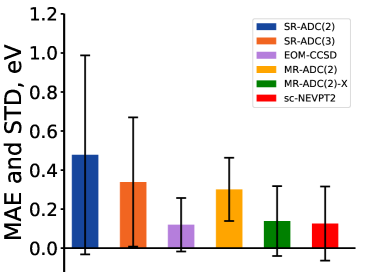
(a)

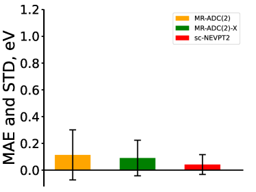
(b)

Figure 4: Mean absolute errors (MAE, eV) and standard deviations from the mean signed error (STD, eV) for vertical electron excitation energies of molecules with (a) equilibrium and (b) stretched geometries, relative to SHCI. MAE is represented as a height of each colored bar, while STD is depicted as a radius of the black vertical line. See Tables 1 and 2 for data on individual molecules with all methods.

Table 2 shows results for electronic excitations of molecules with stretched geometries where the description of multireference effects is important. Unsurprisingly, the accuracy of results produced by the single-reference methods decreases dramatically. In particular, the errors of the single-reference ADC(n) methods become larger with increasing perturbation order (n) as $\Delta_{\mathrm{MAE}}$ roughly doubles from ADC(2) (2.71 eV) to ADC(3) (5.37 eV), while $\Delta_{\mathrm{MAE}}$ for the EOM-CCSD method increases eightfold. The best agreement with SHCI is demonstrated by sc-NEVPT2 ($\Delta_{\mathrm{MAE}}$ = 0.04 eV, $\Delta_{\mathrm{STD}}$ = 0.07 eV). The MR-ADC methods perform similarly well with $\Delta_{\mathrm{MAE}}$ of 0.11 and 0.09 eV for MR-ADC(2) and MR-ADC(2)-X, respectively. The MR-ADC(2)-X approximation shows a smaller $\Delta_{\mathrm{MAX}}$ error (0.37 eV) than that of MR-ADC(2) (0.78 eV), close to $\Delta_{\mathrm{MAX}}$ of sc-NEVPT2 (0.35 eV).

The performance of all methods for this benchmark set is summarized in Figure 4. Overall, our results demonstrate that MR-ADC(2) and MR-ADC(2)-X produce accurate results for many electronic transitions outperforming the single-reference ADC(2) and ADC(3) methods at near-equilibrium geometries and showing accuracy similar to sc-NEVPT2 near dissociation. In contrast to sc-NEVPT2, the MR-ADC methods allow for a straightforward calculation of transition properties (such as oscillator strengths) and do not require using state-averaged CASSCF reference wavefunctions.

5.2 Carbon Dimer

Table 3: Carbon dimer vertical excitation energies ($\Omega$, eV) and oscillator strengths ($f$) computed using the cc-pVDZ basis set with $r$(C-C) = 2.4 $a_{0}$. The MR-ADC and sc-NEVPT2 calculations were performed using the state-specific and state-averaged CASSCF reference wavefunctions, respectively, with the same $(8e,8o)$ active space. Also shown are mean absolute errors ($\Delta_{\mathrm{MAE}}$), standard deviations ($\Delta_{\mathrm{STD}}$), and maximum absolute errors ($\Delta_{\mathrm{MAX}}$) in the computed excitation energies, relative to the DMRG results from Ref. 87.

System	Configuration	Term	sc-NEVPT2	MR-ADC(2)	MR-ADC(2)-X	DMRG
			$\Omega$	$\Omega\ (f)$	$\Omega\ (f)$	$\Omega$
C2	$(2\sigma_{u})^{2}(1\pi_{u})^{3}(3\sigma_{g})^{1}$	${}^{3}\Pi_{u}$	$0.24$	$0.23$	$0.19$	$0.21$
	$(2\sigma_{u})^{2}(1\pi_{u})^{3}(3\sigma_{g})^{1}$	${}^{1}\Pi_{u}$	$1.36$	$1.31$ ($0.003$)	$1.28$ ($0.003$)	$1.29$
	$(2\sigma_{u})^{2}(1\pi_{u})^{2}(3\sigma_{g})^{2}$	${}^{3}\Sigma_{g}^{-}$	$1.33$	$1.27$	$1.25$	$1.29$
	$(2\sigma_{u})^{1}(1\pi_{u})^{4}(3\sigma_{g})^{1}$	${}^{3}\Sigma_{u}^{+}$	$1.33$	$1.53$	$1.38$	$1.29$
	$(2\sigma_{u})^{2}(1\pi_{u})^{2}(3\sigma_{g})^{2}$	${}^{1}\Delta_{g}$	$2.22$	$2.38$	$2.24$	$2.17$
	$(2\sigma_{u})^{2}(1\pi_{u})^{2}(3\sigma_{g})^{2}$	${}^{1}\Sigma_{g}^{+}$	$2.49$	$2.64$	$2.51$	$2.45$
	$(2\sigma_{u})^{1}(1\pi_{u})^{3}(3\sigma_{g})^{2}$	${}^{3}\Pi_{g}$	$2.71$	$2.74$	$2.61$	$2.65$
	$(2\sigma_{u})^{1}(1\pi_{u})^{3}(3\sigma_{g})^{2}$	${}^{1}\Pi_{g}$	$4.72$	$4.71$	$4.61$	$4.61$
	$(2\sigma_{u})^{2}(1\pi_{u})^{3}(1\pi_{g})^{1}$	${}^{3}\Delta_{u}$	$6.96$	$6.79$	$6.60$	$6.66$
$\Delta_{\mathrm{MAE}}$			$0.082$	$0.114$	$0.045$
$\Delta_{\mathrm{STD}}$			$0.084$	$0.093$	$0.055$
$\Delta_{\mathrm{MAX}}$			$0.297$	$0.239$	$0.086$

Next, we consider the C2 molecule, known for the multireference nature of its ground and excited states, which also require accurate description of dynamic correlation.^{92, 93, 94, 95, 87, 81} In our earlier work,²⁶ we demonstrated that the first-order MR-ADC approximation (MR-ADC(1)) captures the strongly correlated nature of the C2 excited states, but produces large errors in vertical excitation energies due to the missing description of the two-electron dynamic correlation effects. Here, we reinvestigate C2 using MR-ADC(2) and MR-ADC(2)-X that provide a more balanced description of static and dynamic correlation.

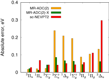
(a)

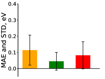
(b)

Figure 5: Absolute errors for vertical excitation energies of C2 (plot (a)), as well as mean absolute errors (MAE) and standard deviations (STD) (plot (b)), relative to DMRG.⁸⁷ In plot (b), the MAE is represented as the height of each colored bar, while STD is depicted as a radius of the black vertical line. See Table 3 for vertical excitation energies.

Table 3 reports the MR-ADC(2), MR-ADC(2)-X, and sc-NEVPT2 vertical excitation energies for C2 at a near equilibrium bond distance ($r$ = 2.4 $a_{0}$) computed using the cc-pVDZ basis set and $(8e,8o)$ active space. The results of these multireference methods are compared to the accurate excitation energies from density matrix renormalization group (DMRG) computed by Wouters et al.⁸⁷ Figure 5 summarizes the performance of each method for predicting the vertical excitation energies of C2. The best agreement with DMRG is shown by MR-ADC(2)-X that reproduces the reference energies with $\Delta_{\mathrm{MAE}}$ and $\Delta_{\mathrm{STD}}$ of $\sim$ 0.05 eV. The sc-NEVPT2 method ($\Delta_{\mathrm{MAE}}$ and $\Delta_{\mathrm{STD}}$ of 0.08 eV) exhibits significantly worse accuracy than MR-ADC(2)-X, but performs slightly better than MR-ADC(2) ($\Delta_{\mathrm{MAE}}$ = 0.11 eV, $\Delta_{\mathrm{STD}}$ = 0.09). The MR-ADC(2) and MR-ADC(2)-X mean absolute errors are reduced tenfold compared to that of MR-ADC(1),²⁶ indicating that the second-order contributions to the MR-ADC propagator are absolutely critical for quantitive predictions of the C2 excited-state energies. As illustrated in Figure 5a, MR-ADC(2)-X has a fairly consistent performance for all excited states resulting in a small $\Delta_{\mathrm{STD}}$, while MR-ADC(2) shows significantly larger errors ($\sim$ 0.2 eV) for the ${}^{3}\Sigma_{u}^{+}$, ${}^{1}\Delta_{g}$, and ${}^{1}\Sigma_{g}^{+}$ states. The errors of sc-NEVPT2 gradually increase reaching $\sim$ 0.3 eV for the highest-energy ${}^{3}\Delta_{u}$ state. The MR-ADC methods predict only one dipole-allowed transition (${}^{1}\Pi_{u}$) with an oscillator strength of 0.003, in agreement with the selection rules of optical spectroscopy.

5.3 Alkenes: Ethylene and Butadiene

Finally, we benchmark MR-ADC(2) and MR-ADC(2)-X for the low-lying excited states of ethylene (C2H4) and butadiene (C4H6). Both molecules have a low-lying triplet state (${}^{3}B_{1u}$ or ${}^{3}B_{u}$), as well as a dipole-allowed $\pi-\pi^{*}$ transition to the singlet state (${}^{1}B_{1u}$ or ${}^{1}B_{u}$) that requires a very accurate description of dynamic correlation between the $\sigma$ and $\pi$ electrons.^{96, 97, 98, 99, 100} In addition, the butadiene molecule features a dipole-forbidden transition to the ${}^{1}A_{g}$ state with a substantial double-excitation character, requiring an accurate description of static correlation in the $\pi$ and $\pi^{*}$ orbitals. For this reason, excitation energies of the butadiene ${}^{1}B_{u}$ and ${}^{1}A_{g}$ states are very sensitive to the level of electron correlation treatment and have been a subject of many theoretical studies.^{98, 99, 100, 101, 102, 103, 104, 105, 106, 107, 108, 109, 88, 110, 42, 111}. In this work, we compute the ethylene and butadiene excited states using MR-ADC(2) and MR-ADC(2)-X and compare their excitation energies to accurate reference results from SHCI obtained by Chien et al.¹⁰⁰ for the same molecular geometries and basis set (see Section 4 for details).

Table 4: Vertical excitation energies (eV) of the ethylene molecule (C2H4) for the lowest-energy triplet state (${}^{3}B_{1u}$) and the lowest-energy dipole-allowed singlet state (${}^{1}B_{1u}$). The MR-ADC results also show the oscillator strength strengths ($f$) in parentheses. See Section 4 for details of the calculations.

Method	Active Space	States
		${}^{3}B_{1u}$	${}^{1}B_{1u}$
EOM-CCSDa		$4.46$	$8.14$
sc-NEVPT2	$(2e,2o)$	$4.84$	$7.68$
	$(2e,4o)$	$4.64$	$8.28$
	$(2e,6o)$	$4.60$	$8.34$
MR-ADC(2)	$(2e,2o)$	$4.85$	$8.19$ ($0.365$)
	$(2e,4o)$	$4.71$	$8.17$ ($0.363$)
	$(2e,6o)$	$4.66$	$8.27$ ($0.363$)
MR-ADC(2)-X	$(2e,2o)$	$4.68$	$7.82$ ($0.338$)
	$(2e,4o)$	$4.56$	$7.92$ ($0.343$)
	$(2e,6o)$	$4.51$	$8.03$ ($0.344$)
SHCIb		$4.59$	$8.05$

• From Ref. 99

• From Ref. 100

Table 4 reports vertical excitation energies for the ${}^{3}B_{u}$ and ${}^{1}B_{u}$ excited states of ethylene computed using MR-ADC(2), MR-ADC(2)-X, sc-NEVPT2, and EOM-CCSD, along with the reference results from SHCI. For the multireference methods we employ three different active spaces ranging from the full-$\pi$ $(2e,2o)$ to the triple-$\pi$ $(2e,6o)$ active space (see the Supporting Information for details). The EOM-CCSD excitation energies are in a good agreement with SHCI with errors less than 0.15 eV, indicating that a high-level description of dynamic correlation is sufficient for accurate description of the ${}^{3}B_{u}$ and ${}^{1}B_{u}$ excited states. Using the minimal $(2e,2o)$ active space, all three multireference methods overestimate the relative energy of the ${}^{3}B_{u}$ state with errors ranging from 0.09 eV (MR-ADC(2)-X) to 0.26 eV (MR-ADC(2)). Increasing the active space lowers the computed ${}^{3}B_{u}$ excitation energy reducing the errors of all three methods to less than 0.1 eV. In contrast, including more $\pi$-orbitals in the active space increases the computed energies of the ${}^{1}B_{u}$ state. Out of all multireference methods, sc-NEVPT2 shows the strongest active-space dependence of the ${}^{1}B_{u}$ excitation energy that changes from 7.68 $(2e,2o)$ to 8.34 eV $(2e,6o)$ and has the worst agreement with SHCI for the largest active space with 0.29 eV error. MR-ADC(2)-X combined with the $(2e,6o)$ active space shows the best agreement with SHCI for the ${}^{1}B_{u}$ state with a small 0.02 eV error. The performance of MR-ADC(2) is similar to that of sc-NEVPT2, although the former method shows a weaker active-space dependence. The ${}^{1}B_{u}$ oscillator strengths computed using the two MR-ADC methods do not change significantly with increasing active space and agree well with each other.

Table 5: Vertical excitation energies (eV) of the butadiene (C4H6) molecule for the lowest-energy triplet state (${}^{3}B_{u}$), as well as the lowest-energy dipole-allowed (${}^{1}B_{u}$) and dipole-forbidden (${}^{1}A_{g}$) singlet states. The MR-ADC results also show the oscillator strength strengths ($f$) in parentheses. See Section 4 for details of the calculations.

Method	Active Space	States
		${}^{3}B_{u}$	${}^{1}B_{u}$	${}^{1}A_{g}$
EOM-CCSDa		$3.20$	$6.53$	$7.28$
sc-NEVPT2	$(4e,4o)$	$3.48$	$5.91$	$6.90$
	$(4e,6o)$	$3.45$	$6.40$	$6.86$
	$(4e,8o)$	$3.43$	$6.54$	$6.77$
MR-ADC(2)	$(4e,4o)$	$3.42$	$6.13$ ($0.619$)	$6.64$
	$(4e,6o)$	$3.56$	$6.46$ ($0.684$)	$6.84$
	$(4e,8o)$	$3.60$	$6.52$ ($0.697$)	$6.91$
MR-ADC(2)-X	$(4e,4o)$	$3.26$	$5.77$ ($0.590$)	$6.20$
	$(4e,6o)$	$3.50$	$6.38$ ($0.670$)	$6.68$
	$(4e,8o)$	$3.54$	$6.39$ ($0.677$)	$6.70$
SHCIb		$3.37$	$6.45$	$6.58$

• From Ref. 99

• From Ref. 100

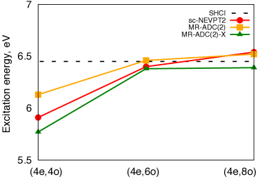
(a)

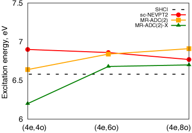
(b)

Figure 6: Vertical excitation energies for the butadiene dipole-allowed ${}^{1}B_{u}$ (plot (a)) and dipole-forbidden ${}^{1}A_{g}$ (plot (b)) electronic states computed using MR-ADC(2), MR-ADC(2)-X, and sc-NEVPT2 as a function of the number of active $\pi$-orbitals ($n$) with 4 active electrons $(4e,no)$. The reference excitation energies computed using SHCI¹⁰⁰ are shown as dashed horizontal lines.

Vertical excitation energies of butadiene are shown in Table 5. As in our study of ethylene, we employ three active spaces for the multireference methods ranging from the full-$\pi$ $(4e,4o)$ to the double-$\pi$ $(4e,8o)$ space. Notably, for this system the EOM-CCSD method shows a large 0.7 eV error for the dipole-forbidden ${}^{1}A_{g}$ state, which is known to have a double-excitation character and requires a multireference treatment. The active-space dependence of the multireference methods for the ${}^{1}A_{g}$ and ${}^{1}B_{u}$ excited states is illustrated in Figure 6. When combined with the smallest $(4e,4o)$ active space, all three multireference methods outperform EOM-CCSD for the ${}^{1}A_{g}$ excitation energy with errors less than 0.4 eV. Using the largest $(4e,8o)$ active space, the best results are shown by MR-ADC(2)-X and sc-NEVPT2 with errors of 0.12 eV and 0.19 eV, respectively. A stronger active-space dependence is observed for the dipole-allowed ${}^{1}B_{u}$ state with the sc-NEVPT2 and MR-ADC(2)-X excitation energies varying by $\sim$ 0.6 eV. Employing the $(4e,8o)$ active space, the best results are shown by MR-ADC(2)-X that outperforms sc-NEVPT2 and EOM-CCSD with an error of 0.06 eV in the ${}^{1}B_{u}$ relative energy. sc-NEVPT2 and MR-ADC(2) overestimate the ${}^{1}B_{u}$ energy by 0.09 and 0.07 eV, respectively. The MR-ADC methods also show a significant active-space dependence in the computed ${}^{1}B_{u}$ oscillator strength that changes by $\sim$ 15 % from $(4e,4o)$ to $(4e,8o)$. A weaker dependence on the active space is observed for the ${}^{3}B_{u}$ state, where the best agreement with SHCI is shown by sc-NEVPT2. Overall, the presented results demonstrate that the MR-ADC methods are competitive in accuracy with sc-NEVPT2 for all three electronic states of butadiene while capable of describing the multireference nature of the ${}^{1}A_{g}$ state that is not captured by EOM-CCSD.

6 Conclusions

In this work, we presented an implementation and benchmark of the strict and extended second-order multireference algebraic diagrammatic construction theory for neutral electronic excitations (MR-ADC(2) and MR-ADC(2)-X). The MR-ADC(2) approximation incorporates all contributions to the polarization propagator up to the second order in its time-independent multireference perturbative expansion, while the MR-ADC(2)-X method includes additional third-order terms in the description of double excitations outside of the active space. We benchmarked the performance of MR-ADC(2) and MR-ADC(2)-X for the excited states in five small molecules (HF, CO, N2, F2, and H2O) at equilibrium and stretched geometries, a carbon dimer (C2), as well as ethylene (C2H4) and butadiene (C4H6).

Our results demonstrate that the MR-ADC methods provide accurate predictions of excited-state energies for the weakly- and strongly-correlated electronic states, at geometric equilibrium or near dissociation. For the weakly-correlated systems, we find that the MR-ADC(2) and MR-ADC(2)-X methods outperform the third-order single-reference ADC approximation (ADC(3)) and are often competitive with the results from equation-of-motion coupled cluster theory (EOM-CCSD). For the multireference problems, the performance of MR-ADC(2) and MR-ADC(2)-X is similar to that of strongly-contracted N-electron valence perturbation theory (sc-NEVPT2). The MR-ADC methods have a number of added benefits, such as a straightforward and efficient calculation of excited-state properties, a direct access to excitations outside of the active space, and an ability to calculate multireference excited states without state-averaged reference wavefunctions.

Our current work can be extended in many possible directions. One important direction is an efficient implementation of the MR-ADC(2) and MR-ADC(2)-X methods that will enable calculations of larger molecular systems with more orbitals and electrons in the active space. Another extension is to take advantage of the MR-ADC ability to calculate excitations outside of the active space, which can be used for efficient calculations of the X-ray absorption spectra of multireference systems. Finally, the methods presented in the current work can be extended to account for relativistic effects, such as spin-orbit and spin-spin coupling, which will enable calculations of magnetic systems with heavy elements. Work along these directions is ongoing in our group.

7 Appendix: Equations for the $t_{x}^{y(2)}$ Amplitudes

As discussed in Section 2.2.2, the MR-ADC(2) and MR-ADC(2)-X second-order effective Hamiltonian $\tilde{H}^{(2)}$ incorporates terms that depend on the internal second-order amplitudes $t_{x}^{y(2)}(x>y)$ that ensure Hermiticity of the effective Hamiltonian matrix $\mathbf{M}$. The $t_{x}^{y(2)}(x>y)$ amplitudes parametrize a contribution to the second-order excitation operator $T^{(2)}$ (Eq. 6) that has the form

$$T^{(2)} \Leftarrow\sum_{x>y}t_{x}^{y(2)}a^{\dagger}_{y}a_{x}$$ (29)

Following our previous work,^{26, 62, 63} the amplitudes $t_{x}^{y(2)}(x>y)$ are obtained by solving the projected linear equations (20) that can be written as:

$$\braket{\Psi_{0}}{a^{\dagger}_{x}a_{y}\tilde{H}^{(2)}}{\Psi_{0}}=0\quad(x>y)$$ (30)

Eq. 30 can be simplified and converted to a tensor form:

$$\mathbf{K}\,\mathbf{T^{(2)}}=-\mathbf{V^{(2)}}$$ (31)

where $\mathbf{T^{(2)}}$ contains $t_{x}^{y(2)}(x>y)$ and the elements of $\mathbf{K}$ and $\mathbf{V^{(2)}}$ are defined as follows:

$$K_{xy,wz} =\braket{\Psi_{0}}{(a^{\dagger}_{x}a_{y}-a^{\dagger}_{y}a_{x})[H^{(0)},a^{\dagger}_{z}a_{w}-a^{\dagger}_{w}a_{z}]}{\Psi_{0}}$$ (32)

$$V_{xy}^{(2)} =\braket{\Psi_{0}}{(a^{\dagger}_{x}a_{y}-a^{\dagger}_{y}a_{x})V^{(2)}}{\Psi_{0}}$$ (33)

Expression for $V^{(2)}$ can be found in Eq. (38) of Ref. 62.

Eq. 31 has the form of the Newton-Raphson equation for the second-order parameters $t_{x}^{y(2)}(x>y)$ that describe relaxation of the active-space orbitals in response to dynamical correlation from outside of the active space. It can be solved by diagonalizing the $\mathbf{K}$ matrix according to the generalized eigenvalue problem

$$\mathbf{K}\,\mathbf{Z}=\mathbf{S}\,\mathbf{Z}\,\boldsymbol{\epsilon}$$ (34)

and inverting the amplitude equation (31) to obtain:

$$\mathbf{T^{(2)}}=-\mathbf{S^{-1/2}}\,\mathbf{\tilde{Z}}\,\boldsymbol{\epsilon^{-1}}\,\mathbf{\tilde{Z}^{\dagger}}\,\mathbf{S^{-1/2}}\,\mathbf{V^{(2)}}\quad(x>y)$$ (35)

In Eqs. 34 and 35 the elements of $\mathbf{S}$ are defined as

$$S_{xy,wz} =\braket{\Psi_{0}}{(a^{\dagger}_{x}a_{y}-a^{\dagger}_{y}a_{x})(a^{\dagger}_{z}a_{w}-a^{\dagger}_{w}a_{z})}{\Psi_{0}}$$ (36)

and $\mathbf{\tilde{Z}}=\mathbf{S^{1/2}}\,\mathbf{Z}$.

Benchmark of the approximation for the second-order amplitudes in Eq. 28. Size-intensivity tests for MR-ADC(2) and MR-ADC(2)-X. Cartesian geometries of the ethylene and butadiene molecules. Active space orbitals in the ethylene and butadiene calculations.

This work was supported by the National Science Foundation under Grant No. CHE-2044648. Computations were performed at the Ohio Supercomputer Center under the projects PAS1583 and PAS1963.¹¹²

References

- Szabo and Ostlund 1982 Szabo, A.; Ostlund, N. S. Modern Quantum Chemistry: Introduction to Advanced Electronic Structure Theory; Macmillan: New York, 1982
- Helgaker et al. 2000 Helgaker, T.; Jørgensen, P.; Olsen, J. Molecular Electronic Structure Theory; John Wiley & Sons, Ltd.: New York, 2000
- Fetter and Walecka 2003 Fetter, A. L.; Walecka, J. D. Quantum theory of many-particle systems; Dover Publications, 2003
- Dickhoff and Van Neck 2005 Dickhoff, W. H.; Van Neck, D. Many-body theory exposed!: Propagator description of quantum mechanics in many-body systems; World Scientific Publishing Co., 2005
- Schirmer 1982 Schirmer, J. Beyond the random-phase approximation: A new approximation scheme for the polarization propagator. Phys. Rev. A 1982, 26, 2395–2416
- Schirmer 1991 Schirmer, J. Closed-form intermediate representations of many-body propagators and resolvent matrices. Phys. Rev. A 1991, 43, 4647
- Mertins and Schirmer 1996 Mertins, F.; Schirmer, J. Algebraic propagator approaches and intermediate-state representations. I. The biorthogonal and unitary coupled-cluster methods. Phys. Rev. A 1996, 53, 2140–2152
- Schirmer and Trofimov 2004 Schirmer, J.; Trofimov, A. B. Intermediate state representation approach to physical properties of electronically excited molecules. J. Chem. Phys. 2004, 120, 11449–11464
- Dreuw and Wormit 2014 Dreuw, A.; Wormit, M. The algebraic diagrammatic construction scheme for the polarization propagator for the calculation of excited states. WIREs Comput. Mol. Sci. 2014, 5, 82–95
- Starcke et al. 2009 Starcke, J. H.; Wormit, M.; Dreuw, A. Unrestricted algebraic diagrammatic construction scheme of second order for the calculation of excited states of medium-sized and large molecules. J. Chem. Phys. 2009, 130, 024104
- Harbach et al. 2014 Harbach, P. H. P.; Wormit, M.; Dreuw, A. The third-order algebraic diagrammatic construction method (ADC(3)) for the polarization propagator for closed-shell molecules: Efficient implementation and benchmarking. J. Chem. Phys. 2014, 141, 064113
- Schirmer et al. 1998 Schirmer, J.; Trofimov, A. B.; Stelter, G. A non-Dyson third-order approximation scheme for the electron propagator. J. Chem. Phys. 1998, 109, 4734
- Trofimov and Schirmer 2005 Trofimov, A. B.; Schirmer, J. Molecular ionization energies and ground- and ionic-state properties using a non-Dyson electron propagator approach. J. Chem. Phys. 2005, 123, 144115
- Angonoa et al. 1987 Angonoa, G.; Walter, O.; Schirmer, J. Theoretical K-shell ionization spectra of N2 and CO by a fourth-order Green’s function method. J. Chem. Phys. 1987, 87, 6789–6801
- Schirmer and Thiel 2001 Schirmer, J.; Thiel, A. An intermediate state representation approach to K-shell ionization in molecules. I. Theory. J. Chem. Phys. 2001, 115, 10621–10635
- Thiel et al. 2003 Thiel, A.; Schirmer, J.; Köppel, H. An intermediate state representation approach to K-shell ionization in molecules. II. Computational tests. J. Chem. Phys. 2003, 119, 2088–2101
- Barth and Schirmer 1985 Barth, A.; Schirmer, J. Theoretical core-level excitation spectra of N2 and CO by a new polarisation propagator method. J. Phys. B: At. Mol. Phys. 1985, 18, 867–885
- Wenzel et al. 2014 Wenzel, J.; Wormit, M.; Dreuw, A. Calculating core-level excitations and X-ray absorption spectra of medium-sized closed-shell molecules with the algebraic-diagrammatic construction scheme for the polarization propagator. J. Comput. Chem. 2014, 35, 1900–1915
- Knippenberg et al. 2012 Knippenberg, S.; Rehn, D. R.; Wormit, M.; Starcke, J. H.; Rusakova, I. L.; Trofimov, A. B.; Dreuw, A. Calculations of nonlinear response properties using the intermediate state representation and the algebraic-diagrammatic construction polarization propagator approach: Two-photon absorption spectra. J. Chem. Phys. 2012, 136, 064107
- Pernpointner 2014 Pernpointner, M. The relativistic polarization propagator for the calculation of electronic excitations in heavy systems. J. Chem. Phys. 2014, 140, 084108
- Krauter et al. 2017 Krauter, C. M.; Schimmelpfennig, B.; Pernpointner, M.; Dreuw, A. Algebraic diagrammatic construction for the polarization propagator with spin-orbit coupling. Chem. Phys. 2017, 482, 286–293
- Pernpointner et al. 2018 Pernpointner, M.; Visscher, L.; Trofimov, A. B. Four-Component Polarization Propagator Calculations of Electron Excitations: Spectroscopic Implications of Spin–Orbit Coupling Effects. J. Chem. Theory Comput. 2018, 14, 1510–1522
- Dempwolff et al. 2019 Dempwolff, A. L.; Schneider, M.; Hodecker, M.; Dreuw, A. Efficient implementation of the non-Dyson third-order algebraic diagrammatic construction approximation for the electron propagator for closed- and open-shell molecules. J. Chem. Phys. 2019, 150, 064108
- Banerjee and Sokolov 2019 Banerjee, S.; Sokolov, A. Y. Third-order algebraic diagrammatic construction theory for electron attachment and ionization energies: Conventional and Green’s function implementation. J. Chem. Phys. 2019, 151, 224112
- Banerjee and Sokolov 2021 Banerjee, S.; Sokolov, A. Y. Efficient implementation of the single-reference algebraic diagrammatic construction theory for charged excitations: Applications to the TEMPO radical and DNA base pairs. J. Chem. Phys. 2021, 154, 074105
- Sokolov 2018 Sokolov, A. Y. Multi-reference algebraic diagrammatic construction theory for excited states: General formulation and first-order implementation. J. Chem. Phys. 2018, 149, 204113
- Wolinski et al. 1987 Wolinski, K.; Sellers, H. L.; Pulay, P. Consistent generalization of the Møller-Plesset partitioning to open-shell and multiconfigurational SCF reference states in many-body perturbation theory. Chem. Phys. Lett. 1987, 140, 225–231
- Hirao 1992 Hirao, K. Multireference Møller—Plesset method. Chem. Phys. Lett. 1992, 190, 374–380
- Werner 1996 Werner, H.-J. Third-order multireference perturbation theory. The CASPT3 method. Mol. Phys. 1996, 89, 645–661
- Finley et al. 1998 Finley, J. P.; Malmqvist, P. Å.; Roos, B. O.; Serrano-Andrés, L. The multi-state CASPT2 method. Chem. Phys. Lett. 1998, 288, 299–306
- Andersson et al. 1990 Andersson, K.; Malmqvist, P. Å.; Roos, B. O.; Sadlej, A. J.; Wolinski, K. Second-order perturbation theory with a CASSCF reference function. J. Phys. Chem. 1990, 94, 5483–5488
- Andersson et al. 1992 Andersson, K.; Malmqvist, P. Å.; Roos, B. O. Second-order perturbation theory with a complete active space self-consistent field reference function. J. Chem. Phys. 1992, 96, 1218–1226
- Angeli et al. 2001 Angeli, C.; Cimiraglia, R.; Evangelisti, S.; Leininger, T.; Malrieu, J.-P. P. Introduction of n-electron valence states for multireference perturbation theory. J. Chem. Phys. 2001, 114, 10252–10264
- Angeli et al. 2001 Angeli, C.; Cimiraglia, R.; Malrieu, J.-P. P. N-electron valence state perturbation theory: a fast implementation of the strongly contracted variant. Chem. Phys. Lett. 2001, 350, 297–305
- Angeli et al. 2004 Angeli, C.; Borini, S.; Cestari, M.; Cimiraglia, R. A quasidegenerate formulation of the second order n-electron valence state perturbation theory approach. J. Chem. Phys. 2004, 121, 4043–4049
- Kurashige and Yanai 2011 Kurashige, Y.; Yanai, T. Second-order perturbation theory with a density matrix renormalization group self-consistent field reference function: Theory and application to the study of chromium dimer. J. Chem. Phys. 2011, 135, 094104
- Kurashige et al. 2014 Kurashige, Y.; Chalupský, J.; Lan, T. N.; Yanai, T. Complete active space second-order perturbation theory with cumulant approximation for extended active-space wavefunction from density matrix renormalization group. J. Chem. Phys. 2014, 141, 174111
- Guo et al. 2016 Guo, S.; Watson, M. A.; Hu, W.; Sun, Q.; Chan, G. K.-L. N-Electron Valence State Perturbation Theory Based on a Density Matrix Renormalization Group Reference Function, with Applications to the Chromium Dimer and a Trimer Model of Poly(p-Phenylenevinylene). J. Chem. Theory Comput. 2016, 12, 1583–1591
- Sokolov and Chan 2016 Sokolov, A. Y.; Chan, G. K.-L. A time-dependent formulation of multi-reference perturbation theory. J. Chem. Phys. 2016, 144, 064102
- Sharma et al. 2017 Sharma, S.; Knizia, G.; Guo, S.; Alavi, A. Combining Internally Contracted States and Matrix Product States To Perform Multireference Perturbation Theory. J. Chem. Theory Comput. 2017, 13, 488–498
- Yanai et al. 2017 Yanai, T.; Saitow, M.; Xiong, X.-G.; Chalupský, J.; Kurashige, Y.; Guo, S.; Sharma, S. Multistate Complete-Active-Space Second-Order Perturbation Theory Based on Density Matrix Renormalization Group Reference States. J. Chem. Theory Comput. 2017, 13, 4829–4840
- Sokolov et al. 2017 Sokolov, A. Y.; Guo, S.; Ronca, E.; Chan, G. K.-L. Time-dependent N-electron valence perturbation theory with matrix product state reference wavefunctions for large active spaces and basis sets: Applications to the chromium dimer and all-trans polyenes. J. Chem. Phys. 2017, 146, 244102
- Chattopadhyay et al. 2000 Chattopadhyay, S.; Mahapatra, U. S.; Mukherjee, D. Development of a linear response theory based on a state-specific multireference coupled cluster formalism. J. Chem. Phys. 2000, 112, 7939–7952
- Chattopadhyay and Mukhopadhyay 2007 Chattopadhyay, S.; Mukhopadhyay, D. Applications of linear response theories to compute the low-lying potential energy surfaces: state-specific MRCEPA-based approach. J. Phys. B: At. Mol. Opt. Phys. 2007, 40, 1787–1799
- Jagau and Gauss 2012 Jagau, T.-C.; Gauss, J. Linear-response theory for Mukherjee’s multireference coupled-cluster method: Excitation energies. J. Chem. Phys. 2012, 137, 044116
- Samanta et al. 2014 Samanta, P. K.; Mukherjee, D.; Hanauer, M.; Köhn, A. Excited states with internally contracted multireference coupled-cluster linear response theory. J. Chem. Phys. 2014, 140, 134108
- Köhn and Bargholz 2019 Köhn, A.; Bargholz, A. The second-order approximate internally contracted multireference coupled-cluster singles and doubles method icMRCC2. J. Chem. Phys. 2019, 151, 041106
- Datta and Nooijen 2012 Datta, D.; Nooijen, M. Multireference equation-of-motion coupled cluster theory. J. Chem. Phys. 2012, 137, 204107
- Nooijen et al. 2014 Nooijen, M.; Demel, O.; Datta, D.; Kong, L.; Shamasundar, K. R.; Lotrich, V.; Huntington, L. M.; Neese, F. Communication: Multireference equation of motion coupled cluster: A transform and diagonalize approach to electronic structure. J. Chem. Phys. 2014, 140, 081102
- Huntington and Nooijen 2015 Huntington, L. M. J.; Nooijen, M. Application of multireference equation of motion coupled-cluster theory to transition metal complexes and an orbital selection scheme for the efficient calculation of excitation energies. J. Chem. Phys. 2015, 142, 194111
- Lechner et al. 2021 Lechner, M. H.; Izsák, R.; Nooijen, M.; Neese, F. A perturbative approach to multireference equation-of-motion coupled cluster. Molecular Physics 2021, 0, e1939185
- Banerjee et al. 1978 Banerjee, A.; Shepard, R.; Simons, J. One-particle Green’s function with multiconfiguration reference states. Int. J. Quantum Chem. 1978, 14, 389–404
- Yeager and Jørgensen 1979 Yeager, D. L.; Jørgensen, P. A multiconfigurational time-dependent Hartree-Fock approach. Chem. Phys. Lett. 1979, 65, 77–80
- Dalgaard 1980 Dalgaard, E. Time-dependent multiconfigurational Hartree–Fock theory. J. Chem. Phys. 1980, 72, 816–823
- Yeager et al. 1984 Yeager, D. L.; Olsen, J.; Jørgensen, P. Generalizations of the multiconfigurational time-dependent Hartree-Fock approach. Faraday Symp. Chem. Soc. 1984, 19, 85–95
- Graham and Yeager 1991 Graham, R. L.; Yeager, D. L. The multiconfigurational particle–particle propagator method for directly determining vertical double ionization potentials and double electron affinities. J. Chem. Phys. 1991, 94, 2884–2893
- Yeager 1992 Yeager, D. L. Applied Many-Body Methods in Spectroscopy and Electronic Structure; Springer, Boston, MA: Boston, MA, 1992; pp 133–161
- Nichols et al. 1984 Nichols, J. A.; Yeager, D. L.; Jørgensen, P. Multiconfigurational electron propagator (MCEP) ionization potentials for general open shell systems. J. Chem. Phys. 1984, 80, 293–314
- Khrustov and Kostychev 2002 Khrustov, V. F.; Kostychev, D. E. Multiconfigurational Green’s function approach with quasidegenerate perturbation theory. Int. J. Quantum Chem. 2002, 88, 507–518
- Helmich-Paris 2019 Helmich-Paris, B. CASSCF linear response calculations for large open-shell molecules. J. Chem. Phys. 2019, 150, 174121
- Helmich-Paris 2021 Helmich-Paris, B. Simulating X-ray absorption spectra with complete active space self-consistent field linear response methods. Int. J. Quantum Chem. 2021, 121, e26559
- Chatterjee and Sokolov 2019 Chatterjee, K.; Sokolov, A. Y. Second-Order Multireference Algebraic Diagrammatic Construction Theory for Photoelectron Spectra of Strongly Correlated Systems. J. Chem. Theory Comput. 2019, 15, 5908–5924
- Chatterjee and Sokolov 2020 Chatterjee, K.; Sokolov, A. Y. Extended Second-Order Multireference Algebraic Diagrammatic Construction Theory for Charged Excitations. J. Chem. Theory Comput. 2020, 16, 6343–6357
- Mukherjee and Kutzelnigg 1989 Mukherjee, D.; Kutzelnigg, W. Many-Body Methods in Quantum Chemistry; Springer, Berlin, Heidelberg: Berlin, Heidelberg, 1989; pp 257–274
- Lehmann 1954 Lehmann, H. Über Eigenschaften von Ausbreitungsfunktionen und Renormierungskonstanten quantisierter Felder. Nuovo Cim 1954, 11, 342–357
- Kirtman 1981 Kirtman, B. Simultaneous calculation of several interacting electronic states by generalized Van Vleck perturbation theory. J. Chem. Phys. 1981, 75, 798–808
- Hoffmann and Simons 1988 Hoffmann, M. R. R.; Simons, J. A unitary multiconfigurational coupled-cluster method: Theory and applications. J. Chem. Phys. 1988, 88, 993
- Yanai and Chan 2006 Yanai, T.; Chan, G. K.-L. Canonical transformation theory for multireference problems. J. Chem. Phys. 2006, 124, 194106
- Chen and Hoffmann 2012 Chen, Z.; Hoffmann, M. R. R. Orbitally invariant internally contracted multireference unitary coupled cluster theory and its perturbative approximation: Theory and test calculations of second order approximation. J. Chem. Phys. 2012, 137, 014108
- Li and Evangelista 2015 Li, C.; Evangelista, F. A. Multireference Driven Similarity Renormalization Group: A Second-Order Perturbative Analysis. J. Chem. Theory Comput. 2015, 11, 2097–2108
- Malmqvist and Roos 1989 Malmqvist, P.-Å.; Roos, B. O. The CASSCF state interaction method. Chem. Phys. Lett. 1989, 155, 189 – 194
- Dyall 1995 Dyall, K. G. The choice of a zeroth-order Hamiltonian for second-order perturbation theory with a complete active space self-consistent-field reference function. J. Chem. Phys. 1995, 102, 4909–4918
- Löwdin 1985 Löwdin, P. O. Some Aspects on the Hamiltonian and Liouvillian Formalism, the Special Propagator Methods, and the Equation of Motion Approach. Adv. Quant. Chem. 1985, 17, 285–334
- Kutzelnigg and Mukherjee 1989 Kutzelnigg, W.; Mukherjee, D. Time-independent theory of one-particle Green’s functions. J. Chem. Phys. 1989, 90, 5578–5594
- Davidson 1975 Davidson, E. R. The iterative calculation of a few of the lowest eigenvalues and corresponding eigenvectors of large real-symmetric matrices. J. Comput. Phys. 1975, 17, 87
- Liu 1978 Liu, B. The Simultaneous Expansion Method for the Iterative Solution of Several of the Lowest-Lying Eigenvalues and Corresponding Eigenvectors of Large Real-Symmetric Matrices; 1978
- Neuscamman et al. 2009 Neuscamman, E.; Yanai, T.; Chan, G. K.-L. Quadratic canonical transformation theory and higher order density matrices. J. Chem. Phys. 2009, 130, 124102
- Sun et al. 2020 Sun, Q.; Zhang, X.; Banerjee, S.; Bao, P.; Barbry, M.; Blunt, N. S.; Bogdanov, N. A.; Booth, G. H.; Chen, J.; Cui, Z.-H.; Eriksen, J. J.; Gao, Y.; Guo, S.; Hermann, J.; Hermes, M. R.; Koh, K.; Koval, P.; Lehtola, S.; Li, Z.; Liu, J.; Mardirossian, N.; McClain, J. D.; Motta, M.; Mussard, B.; Pham, H. Q.; Pulkin, A.; Purwanto, W.; Robinson, P. J.; Ronca, E.; Sayfutyarova, E. R.; Scheurer, M.; Schurkus, H. F.; Smith, J. E. T.; Sun, C.; Sun, S.-N.; Upadhyay, S.; Wagner, L. K.; Wang, X.; White, A. F.; Whitfield, J. D.; Williamson, M. J.; Wouters, S.; Yang, J.; Yu, J. M.; Zhu, T.; Berkelbach, T. C.; Sharma, S.; Sokolov, A. Y.; Chan, G. K.-L. Recent developments in the PySCF program package. J. Chem. Phys. 2020, 153, 024109
- Holmes et al. 2016 Holmes, A. A.; Tubman, N. M.; Umrigar, C. J. Heat-Bath Configuration Interaction: An Efficient Selected Configuration Interaction Algorithm Inspired by Heat-Bath Sampling. J. Chem. Theory Comput. 2016, 12, 3674–3680
- Sharma et al. 2017 Sharma, S.; Holmes, A. A.; Jeanmairet, G.; Alavi, A.; Umrigar, C. J. Semistochastic Heat-Bath Configuration Interaction Method: Selected Configuration Interaction with Semistochastic Perturbation Theory. J. Chem. Theory Comput. 2017, 13, 1595–1604
- Holmes et al. 2017 Holmes, A. A.; Umrigar, C. J.; Sharma, S. Excited states using semistochastic heat-bath configuration interaction. J. Chem. Phys. 2017, 147, 164111
- Geertsen et al. 1989 Geertsen, J.; Rittby, M.; Bartlett, R. J. The equation-of-motion coupled-cluster method: Excitation energies of Be and CO. Chem. Phys. Lett. 1989, 164, 57–62
- Comeau and Bartlett 1993 Comeau, D. C.; Bartlett, R. J. The equation-of-motion coupled-cluster method. Applications to open- and closed-shell reference states. Chem. Phys. Lett. 1993, 207, 414–423
- Stanton and Bartlett 1993 Stanton, J. F.; Bartlett, R. J. The equation of motion coupled-cluster method. A systematic biorthogonal approach to molecular excitation energies, transition probabilities, and excited state properties. J. Chem. Phys. 1993, 98, 7029
- Krylov 2008 Krylov, A. I. Equation-of-Motion Coupled-Cluster Methods for Open-Shell and Electronically Excited Species: The Hitchhiker’s Guide to Fock Space. Annu. Rev. Phys. Chem. 2008, 59, 433–462
- Shao et al. 2014 Shao, Y.; Gan, Z.; Epifanovsky, E.; Gilbert, A. T. B.; Wormit, M.; Kussmann, J.; Lange, A. W.; Behn, A.; Deng, J.; Feng, X.; Ghosh, D.; Goldey, M.; Horn, P. R.; Jacobson, L. D.; Kaliman, I.; Khaliullin, R. Z.; Kuś, T.; Landau, A.; Liu, J.; Proynov, E. I.; Rhee, Y. M.; Richard, R. M.; Rohrdanz, M. A.; Steele, R. P.; Sundstrom, E. J.; Woodcock III, H. L.; Zimmerman, P. M.; Zuev, D.; Albrecht, B.; Alguire, E.; Austin, B.; Beran, G. J. O.; Bernard, Y. A.; Berquist, E.; Brandhorst, K.; Bravaya, K. B.; Brown, S. T.; Casanova, D.; Chang, C.-M.; Chen, Y.; Chien, S. H.; Closser, K. D.; Crittenden, D. L.; Diedenhofen, M.; Distasio JR., R. A.; Do, H.; Dutoi, A. D.; Edgar, R. G.; Fatehi, S.; Fusti-Molnar, L.; Ghysels, A.; Golubeva-Zadorozhnaya, A.; Gomes, J.; Hanson-Heine, M. W. D.; Harbach, P. H. P.; Hauser, A. W.; Hohenstein, E. G.; Holden, Z. C.; Jagau, T.-C.; Ji, H.; Kaduk, B.; Khistyaev, K.; Kim, J.; Kim, J.; King, R. A.; Klunzinger, P.; Kosenkov, D.; Kowalczyk, T.; Krauter, C. M.; Lao, K. U.; Laurent, A. D.; Lawler, K. V.; Levchenko, S. V.; Lin, C. Y.; Liu, F.; Livshits, E.; Lochan, R. C.; Luenser, A.; Manohar, P.; Manzer, S. F.; Mao, S.-P.; Mardirossian, N.; Marenich, A. V.; Maurer, S. A.; Mayhall, N. J.; Neuscamman, E.; Oana, C. M.; Olivares-Amaya, R.; O’Neill, D. P.; Parkhill, J. A.; Perrine, T. M.; Peverati, R.; Prociuk, A.; Rehn, D. R.; Rosta, E.; Russ, N. J.; Sharada, S. M.; Sharma, S.; Small, D. W.; Sodt, A.; Stein, T.; Stück, D.; Su, Y.-C.; Thom, A. J. W.; Tsuchimochi, T.; Vanovschi, V.; Vogt, L.; Vydrov, O.; Wang, T.; Watson, M. A.; Wenzel, J.; White, A. F.; Williams, C. F.; Yang, J.; Yeganeh, S.; Yost, S. R.; You, Z.-Q.; Zhang, I. Y.; Zhang, X.; Zhao, Y.; Brooks, B. R.; Chan, G. K.-L.; Chipman, D. M.; Cramer, C. J.; Goddard III, W. A.; Gordon, M. S.; Hehre, W. J.; Klamt, A.; Schaefer, H. F.; Schmidt, M. W.; Sherrill, C. D.; Truhlar, D. G.; Warshel, A.; Xu, X.; Aspuru-Guzik, A.; Baer, R.; Bell, A. T.; Besley, N. A.; Chai, J.-D.; Dreuw, A.; Dunietz, B. D.; Furlani, T. R.; Gwaltney, S. R.; Hsu, C.-P.; Jung, Y.; Kong, J.; Lambrecht, D. S.; Liang, W.; Ochsenfeld, C.; Rassolov, V. A.; Slipchenko, L. V.; Subotnik, J. E.; Van Voorhis, T.; Herbert, J. M.; Krylov, A. I.; Gill, P. M. W.; Head-Gordon, M. Advances in molecular quantum chemistry contained in the Q-Chem 4 program package. Mol. Phys. 2014, 113, 184–215
- Wouters et al. 2014 Wouters, S.; Poelmans, W.; Ayers, P. W.; Van Neck, D. CheMPS2: A free open-source spin-adapted implementation of the density matrix renormalization group for ab initio quantum chemistry. Comput. Phys. Commun. 2014, 185, 1501–1514
- Daday et al. 2012 Daday, C.; Smart, S.; Booth, G. H.; Alavi, A.; Filippi, C. Full Configuration Interaction Excitations of Ethene and Butadiene: Resolution of an Ancient Question. J. Chem. Theory Comput. 2012, 8, 4441–4451
- Kendall et al. 1992 Kendall, R. A.; Dunning Jr, T. H.; Harrison, R. J. Electron affinities of the first-row atoms revisited. Systematic basis sets and wave functions. J. Chem. Phys. 1992, 96, 6796–6806
- Dunning Jr 1989 Dunning Jr, T. H. Gaussian basis sets for use in correlated molecular calculations. I. The atoms boron through neon and hydrogen. J. Chem. Phys. 1989, 90, 1007–1023
- Widmark et al. 1990 Widmark, P.-O.; Malmqvist, P. Å.; Björn O Roos, Density matrix averaged atomic natural orbital (ANO) basis sets for correlated molecular wave functions. Theoret. Chim. Acta 1990, 77, 291–306
- Roos 1987 Roos, B. O. The Complete Active Space Self-Consistent Field Method and its Applications in Electronic Structure Calculations. Adv. Chem. Phys. 1987, 69, 399–445
- Bauschlicher Jr and Langhoff 1987 Bauschlicher Jr, C. W.; Langhoff, S. R. Ab initio calculations on C2, Si2, and SiC. J. Chem. Phys. 1987, 87, 2919
- Watts and Bartlett 1998 Watts, J. D.; Bartlett, R. J. Coupled-cluster calculations on the C2 molecule and the C and C molecular ions. J. Chem. Phys. 1998, 96, 6073–6084
- Abrams and Sherrill 2004 Abrams, M. L.; Sherrill, C. D. Full configuration interaction potential energy curves for the X1, B1g, and B states of C2: A challenge for approximate methods. J. Chem. Phys. 2004, 121, 9211
- Davidson 1996 Davidson, E. R. The Spatial Extent of the V State of Ethylene and Its Relation to Dynamic Correlation in the Cope Rearrangement. J. Phys. Chem. 1996, 100, 6161–6166
- Angeli 2010 Angeli, C. An analysis of the dynamic polarization in the V state of ethene. Int. J. Quantum Chem. 2010, 110, 2436–2447
- Watts et al. 1996 Watts, J. D.; Gwaltney, S. R.; Bartlett, R. J. Coupled-cluster calculations of the excitation energies of ethylene, butadiene, and cyclopentadiene. J. Chem. Phys. 1996, 105, 6979–6988
- Copan and Sokolov 2018 Copan, A. V.; Sokolov, A. Y. Linear-Response Density Cumulant Theory for Excited Electronic States. J. Chem. Theory Comput. 2018, 14, 4097–4108
- Chien et al. 2018 Chien, A. D.; Holmes, A. A.; Otten, M.; Umrigar, C. J.; Sharma, S.; Zimmerman, P. M. Excited States of Methylene, Polyenes, and Ozone from Heat-Bath Configuration Interaction. J. Phys. Chem. A 2018, 122, 2714–2722
- Tavan and Schulten 1986 Tavan, P.; Schulten, K. The low-lying electronic excitations in long polyenes: A PPP-MRD-CI study. 1986, 85, 6602–6609
- Tavan and Schulten 1987 Tavan, P.; Schulten, K. Electronic excitations in finite and infinite polyenes. Phys. Rev. B 1987, 36, 4337–4358
- Nakayama et al. 1998 Nakayama, K.; Nakano, H.; Hirao, K. Theoretical study of the →* excited states of linear polyenes: The energy gap between 11Bu+ and 21Ag− states and their character. Int. J. Quantum Chem. 1998, 66, 157–175
- Li and Paldus 1999 Li, X.; Paldus, J. Size dependence of the X1Ag→11Bu excitation energy in linear polyenes. Int. J. Quantum Chem. 1999, 74, 177–192
- Kurashige et al. 2004 Kurashige, Y.; Nakano, H.; Nakao, Y.; Hirao, K. The →* excited states of long linear polyenes studied by the CASCI-MRMP method. Chem. Phys. Lett. 2004, 400, 425–429
- Starcke et al. 2006 Starcke, J. H.; Wormit, M.; Schirmer, J.; Dreuw, A. How much double excitation character do the lowest excited states of linear polyenes have? Chem. Phys. 2006, 329, 39–49
- Ghosh et al. 2008 Ghosh, D.; Hachmann, J.; Yanai, T.; Chan, G. K.-L. Orbital optimization in the density matrix renormalization group, with applications to polyenes and -carotene. 2008, 128, 144117
- Schreiber et al. 2008 Schreiber, M.; Silva-Junior, M. R.; Sauer, S. P. A.; Thiel, W. Benchmarks for electronically excited states: CASPT2, CC2, CCSD, and CC3. J. Chem. Phys. 2008, 128, 134110
- Zgid et al. 2009 Zgid, D.; Ghosh, D.; Neuscamman, E.; Chan, G. K.-L. A study of cumulant approximations to n-electron valence multireference perturbation theory. J. Chem. Phys. 2009, 130, 194107
- Watson and Chan 2012 Watson, M. A.; Chan, G. K.-L. Excited States of Butadiene to Chemical Accuracy: Reconciling Theory and Experiment. J. Chem. Theory Comput. 2012, 8, 4013–4018
- Zimmerman 2017 Zimmerman, P. M. Singlet–Triplet Gaps through Incremental Full Configuration Interaction. J. Phys. Chem. A 2017, 121, 4712–4720
- Ohi 1987 Ohio Supercomputer Center; 1987