Origin of metals in old Milky Way halo stars based on GALAH and Gaia

Abstract

Stellar and supernova nucleosynthesis in the first few billion years of the cosmic history have set the scene for early structure formation in the Universe, while little is known about their nature. Making use of stellar physical parameters measured by GALAH Data Release 3 with accurate astrometry from the Gaia EDR3, we have selected $\sim 100$ old main-sequence turn-off stars (ages $\gtrsim 12$ Gyrs) with kinematics compatible with the Milky Way stellar halo population in the Solar neighborhood. Detailed homogeneous elemental abundance estimates by GALAH DR3 are compared with supernova yield models of Pop III (zero-metal) core-collapse supernovae (CCSNe), normal (non-zero-metal) CCSNe, and Type Ia supernovae (SN Ia) to examine which of the individual yields or their combinations best reproduce the observed elemental abundance patterns for each of the old halo stars (“OHS”). We find that the observed abundances in the OHS with [Fe/H]$>-1.5$ are best explained by contributions from both CCSNe and SN Ia, where the fraction of SN Ia among all the metal-enriching SNe is up to 10–20 % for stars with high [Mg/Fe] ratios and up to 20–27 % for stars with low [Mg/Fe] ratios, depending on the assumption about the relative fraction of near-Chandrasekhar-mass SNe Ia progenitors. The results suggest that, in the progenitor systems of the OHS with [Fe/H]$>-1.5$, $\sim$ 50–60% of Fe mass originated from normal CCSNe at the earliest phases of the Milky Way formation. These results provide an insight into the birth environments of the oldest stars in the Galactic halo.

1 Introduction

Production of elements by stars and supernovae in the first few billion years of the cosmic history had impacted the environment of star formation in the early Universe (Bromm & Larson, 2004; Greif et al., 2010; Bromm & Yoshida, 2011; Karlsson et al., 2013). After the Big Bang nucleosynthesis, the first stars, so called Population III (Pop III) stars, were formed as a result of condensation of primordial, pure H and He gas in cosmological mini-halos driven by cooling via molecular hydrogen (e.g., Bromm & Larson, 2004). Depending on the initial stellar masses, Pop III stars undergo supernova explosions and have enriched the primordial gas with metals for the first time in the cosmic history (Umeda & Nomoto, 2002; Heger & Woosley, 2002, 2010; Limongi & Chieffi, 2012; Nomoto et al., 2013; Ishigaki et al., 2018).

Once a critical metal or dust abundance is reached, gas cooling becomes more efficient, which leads to the formation of stars with masses more typical of the present-day Universe (e.g., Bromm & Yoshida, 2011; Chiaki et al., 2014). The stars with masses in the range $\sim 10-40~{}M_{\odot}$ mainly synthesize elements from carbon to silicon through their hydrostatic burning and eject the nucleosynthetic products by core-collapse supernovae (CCSNe) (e.g., Woosley & Weaver, 1995; Thielemann et al., 1996; Nomoto et al., 2013). These normal CCSNe (progenitors with non-zero metal contents) further chemically enrich the interstellar medium. Stars with masses below $\sim 8~{}M_{\odot}$ evolve into a white dwarf, which is a potential progenitor of a Type Ia supernova (SN Ia) (e.g., Umeda et al., 1999; Kobayashi et al., 2020b). The SNe Ia are mainly responsible for production of Fe-group elements, such that 60 % of Fe in the Solar system material is originated from SN Ia (Kobayashi et al. 2020a, see also Tsujimoto et al. 1995).

The chemical enrichment processes by these nucleosynthetic channels in the early galactic environments are still elusive. The physical properties of Pop III stars are one of the biggest uncertainties regarding the early cosmic chemical evolution. Cosmological simulations predict several orders of magnitudes difference in characteristic masses of the Pop III stars ranging from more than $\sim$100$~{}M_{\odot}$ (Bromm et al., 2002; O’Shea & Norman, 2007; Yoshida et al., 2006), a few tens of $M_{\odot}$ (Stacy et al., 2010, 2012; Hosokawa et al., 2011; Sharda et al., 2019), down to less than a few $M_{\odot}$ (Clark et al., 2011; Greif et al., 2011; Stacy & Bromm, 2014). A few orders of magnitudes spread in the predicted Pop III masses and their multiplicity have also been predicted (Hirano et al., 2014, 2015; Susa et al., 2014; Susa, 2019; Sugimura et al., 2020). In addition to the masses, presence of stellar rotation could also impact the metal yields as well as the overall evolution of the progenitor stars (Meynet et al., 2006; Hirschi, 2007; Joggerst et al., 2010; Takahashi et al., 2014; Limongi & Chieffi, 2018; Choplin et al., 2019).

In addition to the Pop III properties, it remains unclear how the ejected metals from Pop III supernovae are transported in the inter galactic medium (IGM) and mixed with primordial gas, from which the next generation, namely, the first metal-enriched stars formed (e.g., Smith et al., 2009; Ritter et al., 2012; Chiaki et al., 2018; Tarumi et al., 2020). Such mechanisms can depend on multiplicity of Pop III stars (Hartwig et al., 2018; Hartwig et al., 2019) or presence of radiative feedback from the Pop III stars (Greif et al., 2010; Jeon et al., 2014; Cooke & Madau, 2014; Chiaki et al., 2018).

Physical mechanisms of CCSN explosions of massive stars in general are crucial for the final yields, while they are not well understood (e.g., Janka, 2012). The explosive nucleosynthesis, amount of fallback (e.g., Woosley & Weaver, 1995; Thielemann et al., 1996; Zhang et al., 2008), mixing in ejecta (e.g., Joggerst et al., 2009), and departure from spherical symmetry (e.g., Tominaga, 2009; Ezzeddine et al., 2019) can all affect the nucleosynthesis products that ultimately contribute to the chemical enrichment.

Finally, progenitor systems of SNe Ia have not been identified. SN Ia is a thermonuclear explosion of a white dwarf of carbon-oxygen composition. A minimum possible time scale is thus determined by an age of the most massive white dwarf progenitors, which corresponds to a few tens of Myrs for $\sim 8~{}M_{\odot}$ stars. Whether a white dwarf is able to explode as a SN Ia depends on properties of the host binary system, which determines mass accretion from the companion star (Single-Degenerate or SD scenario Nomoto, 1982) or on the possibility of a merger of two white dwarfs within a reasonable timescale (Double-Degenerate or DD scenario, e.g., Hillebrandt & Niemeyer, 2000). These scenarios are observationally tested, for example, through characteristic delay time for SNe Ia relative to a major star formation episode. The characteristic delay time or the delay-time distribution has been addressed at various environments and redshifts, while a clear consensus about the dominant SN Ia channel has not been obtained (e.g., Hopkins & Beacom, 2006; Totani et al., 2008; Hachisu et al., 2008; Maoz et al., 2014). In both the SD and DD scenarios, nucleosynthetic yields of SN Ia are mainly determined by physical conditions such as matter density at which thermonuclear burning is ignited, which depends on masses of white dwarfs at the onset of explosion (e.g., Nomoto et al., 1984; Thielemann et al., 1986; Sato et al., 2015, 2016; Kobayashi et al., 2020a). According to this mass, nucleosynthetic products of SN Ia are often categorized according to whether the mass of a white dwarf SN Ia progenitor is close to or below the Chandrasekhar white dwarf mass limit, $M_{\rm Ch}\sim 1.4~{}M_{\odot}$. For some elements, the nucleosynthetic yields of SN Ia are largely different between near-$M_{\rm Ch}$ or sub-$M_{\rm Ch}$ white dwarf progenitor models (e.g., Nomoto & Leung, 2018; Leung & Nomoto, 2018, 2020).

Since it is not feasible to directly observe processes of metal enrichment at high redshifts, the only observational probe of the metal-enrichment sources in the early Universe has been chemical signatures retained in the atmosphere of nearby long-lived stars in the Milky Way halo. Stars with the lowest Fe abundances such as extremely metal-poor (EMP) stars with [Fe/H]$<-3$ are commonly considered to be objects retaining chemical signatures of the Pop III nucloesynthesis (Beers & Christlieb, 2005; Frebel & Norris, 2015). Stars with a wider range of [Fe/H] can also be used as an important probe of chemical evolution as a function of cosmic time by comparing with chemical evolution models (e.g., Kobayashi et al., 2006, 2020b).

While the [Fe/H] abundance is frequently used as a proxy for stellar ages for Galactic halo stars, it has been shown that the age-[Fe/H] relationship depends on the star formation environment. In fact, the Galactic bulge is known to host very old stellar populations, including globular clusters with an age as old as the age of the Universe (e.g., Barbuy et al., 2018, and references therein). Cosmological simulations that implement chemical evolution models also predict that the oldest stars in various Galactic environments do not exclusively possess very low Fe abundances (e.g., Salvadori et al., 2010; Starkenburg et al., 2017; El-Badry et al., 2018; Salvadori et al., 2019). Instead, stellar ages are a fundamental property to identify stars more likely formed in the early Universe, and thus, under the influence of chemical enrichment by the earliest generations of stars. The stellar ages, however, are extremely difficult to estimate for a single star and are often suffer from large systematic uncertainty or dependent on assumptions in stellar evolution modeling (Soderblom, 2010). It has become feasible only recently to obtain stellar ages for a large homogeneous sample of stars thanks to large surveys of Galactic stellar populations (e.g., Sanders & Das, 2018; Sharma et al., 2020). The stars with age, kinematics and chemical abundance estimates available from these massive surveys motivate us to address the question whether there are old but comparatively metal-rich nearby halo stars which possess chemical signatures of the metal enrichment by the earliest generations of stars.

In this paper, we select candidates of old stars in the Milky Way halo based on stellar ages and kinematics provided by the most up-to-date data releases of the Galactic Archaeology with HERMES (GALAH) survey (De Silva et al., 2015; Buder et al., 2021) and the Gaia mission (Lindegren et al., 2020). For the selected stars, we compare observed elemental abundance patterns with sets of yield models for Pop III CCSNe, normal (non-zero-metal 10–40$~{}M_{\odot}$) CCSNe and SNe Ia.

This paper is organized as follows. Section 2 describes the sample selection method based on the GALAH and Gaia data. Section 3 describes the yield models we use to fit the observed elemental abundances. Section 4 presents results of fitting the yield models to the observed abundances. Section 5 gives implications of the results on the metal-enrichment in the early Galactic environment. Finally, we give a summary and our conclusions in Section 6.

2 Data

In this paper, we base our analysis on stellar parameters, elemental abundances, and age estimates from GALAH DR3 (Buder et al., 2021). The main catalog of GALAH DR3 provides stellar parameters and elemental abundances for 588,571 stars obtained using both astrometric data from Gaia DR2 and spectroscopic data from the GALAH survey itself. We further make use of one of the Value-Added Catalogs, which provides age estimates (See Section 2.2.1). To calculate stellar orbital parameters, GALAH DR3 catalog is cross-matched with Gaia EDR3 (Lindegren et al., 2020), which provides up-to-date astrometric data for most of the GALAH DR3 stars. In the following subsections, we first describe the adopted quality cuts. We then describe the sample selection criteria by age and kinematics.

2.1 Quality cuts

2.1.1 GALAH DR3

We applied the following cuts to select stars that are candidates of old stars with reliable stellar parameter and age estimates from the main and the Value-Added Catalog of GALAH DR3 (Buder et al., 2021).

First, we adopt a criterion, flag_sp=0, to ensure that stars have reliable astrometry from Gaia DR2 and with no issues raised in the data reduction process regarding either data quality, peculiar spectral properties (e.g., binary or emission line stars) or large $\chi^{2}$ in the fitting (for the full list, see Table 6 of Buder et al. 2021). Next, $S/N=$SNR_C2_IRAF $>40$ is applied to select stars with precise stellar parameter estimates. At SNR_C2_IRAF $=40$, Buder et al. (2021) report that the typical precision of $T_{\rm eff}$, $\log g$, and [Fe/H] are 49 K, 0.07 dex, and 0.055 dex, respectively. We further restrict our analysis to main-sequence turn-off (MSTO) stars by requiring $3.2<\verb|logg|<4.1$ and $5000<\verb|teff|<7000$, which is the same as the MSTO selection criteria adopted in Sharma et al. (2021). Finally, we require that more than five measurements of [X/Fe], except for Ti or Sc, are available. This ensures that the model parameters (see Section 3) can be robustly constrained by the measured abundance ratios.

To summarize, we adopt following quality cuts:

• flag_sp=0 (73%)

• $S/N=$SNR_C2_IRAF $>40$ (29%)

• $3.2<\verb|logg|<4.1$ & $5000<\verb|teff|<7000$ (7%)

• More than five [X/Fe] measurements. (7%)

Numbers in the brackets indicate the percentage of remaining stars relative to all stars in the main catalog after additionally applying each cut.

2.1.2 Gaia EDR3

The selected stars are cross matched with the Gaia EDR3 (Lindegren et al., 2020) to obtain accurate astrometric data for the kinematic selection in Section 2.2.2. We restrict our sample to stars with high astrometric quality by requiring ruwe $<1.4$ as recommended in Lindegren (2018), where the value of ruwe (re-normalized unit weight error) quantifies the chi-square of the astrometric fit. We also exclude stars with negative parallaxes or with parallax_error/parallax$\geq 0.1$, to exclude objects with unreliable distance estimates. After the above quality cuts, $\sim 35,000$ stars ($\sim 6\%$ of the entire GALAH DR3 catalog) remain.

2.2 Sample selection

2.2.1 Age

In order to select old star candidates in the GALAH-Gaia cross-matched catalog described in the previous section, we employ stellar ages from the Value-Added Catalog of GALAH DR3 (Buder et al., 2021). Stellar ages in this catalog have been estimated by the Bayesian Stellar Parameter Estimation code, BSTEP, developed by Sharma et al. (2018). The code makes use of observed stellar parameters ($T_{\rm eff}$ and $\log g$), chemical composition ([Fe/H] and [$\alpha$/Fe]), photometry (2MASS $J$ and $K_{s}$) and astrometry (parallax) to be compared with theoretical isochrone models (Buder et al., 2021). For the isochrone models, PARSEC-v1.2S (Bressan et al., 2012) with 121 age grid points spanning $6.6<\log{\rm age/Gyr}<10.12$ were used (Sharma et al., 2018; Buder et al., 2021). A flat prior on age across $0<{\rm age/Gyr}<13.18$ has been adopted (Sharma et al., 2018). For an estimate of age and its statistical uncertainty in the catalog, a mean and a standard deviation based on 16 and 84 percentiles are reported (Buder et al., 2021). Figure 1 shows histograms of the one-sigma age uncertainties reported in GALAH DR3 for the stars that satisfy the quality cuts in Section 2.1 (the gray histogram) and the age-kinematics cut described in this and the next section (the cyan and red histograms). The median value of the age uncertainties for the stars that satisfy the quality cut is 0.7 Gyrs. We note that the age uncertainties have been obtained assuming the flat age prior, which could be a strong prior. Given that typical ages of nearby field Milky Way stellar halo have been estimated to be $>10$ Gyrs (e.g., Gallart et al., 2019), we adopt an age cut of $>12$ Gyrs to select candidates of very old stars in the Solar neighborhood.

Figure 2 shows $T_{\rm eff}$-$\log g$ diagrams for stars that satisfy the age cut (cyan crosses) for three different [Fe/H] ranges. A typical uncertainty of $T_{\rm eff}$ and $\log g$ in the GALAH DR3 catalog for the age-selected sample is shown at the left bottom in each panel. For each [Fe/H] range, theoretical isochrones from the Dartmouth Stellar Evolution Database (Dotter et al., 2008) with ages 5, 10, 12, and 14 Gyrs with a scaled-solar $\alpha$-element abundance are shown (black dash-dotted, dashed, dotted and solid lines, respectively). As can be seen, the age-selected sample is mostly cooler than the oldest isochrone model. Since a sizable fraction of the sample is enhanced in [$\alpha$/Fe] in the range 0.0-0.4 (see Section 2.2.3), Figure 2 also shows isochrones with an enhanced $\alpha$-element abundance of [$\alpha$/Fe] = 0.4. It can be seen that, for a given [Fe/H] and an age, the $\alpha$-enhanced models are cooler than the corresponding $\alpha$-solar models and therefore, the absolute age estimates could be a subject of systematic uncertainties depending on [$\alpha$/Fe] abundance ratios of individual stars. Because of the possible systematic uncertainties in absolute ages, our age-selected sample should be interpreted as the oldest stars among those observed by GALAH DR3 and Gaia EDR3 in the Solar neighborhood.

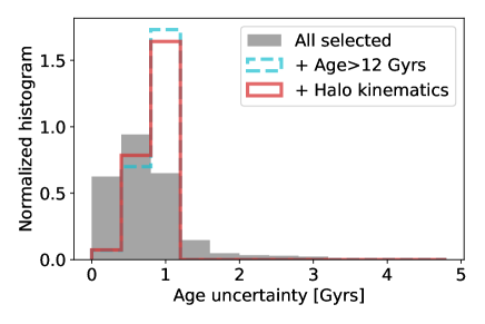
Figure 1: Normalized histograms of the one-sigma age uncertainties from the GALAH DR3 catalog for the sample of stars selected for this study. The gray histogram corresponds to all $\sim 35,000$ stars that satisfy the quality cuts in Section 2.1. The age-selected sample (Section 2.2.1 is shown by the cyan dashed histogram. The stars that satisfy both the age and kinematic criteria (Section 2.2.2) are shown by the red solid histogram.

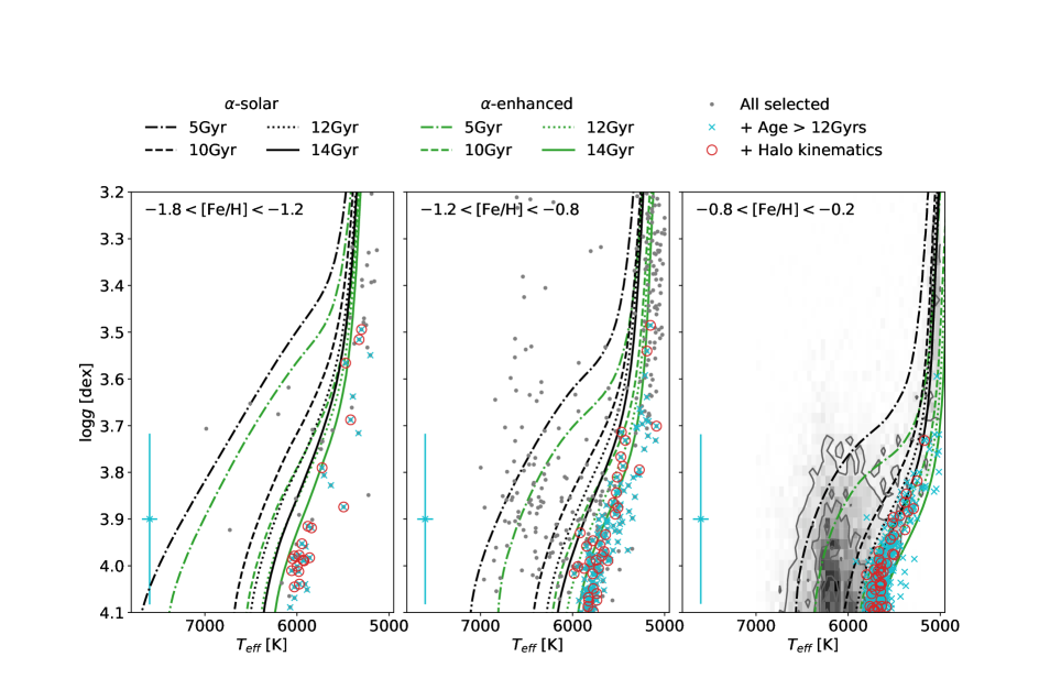
Figure 2: The $T_{\rm eff}-\log g$ diagrams for the sample stars with [Fe/H] metallicities in the ranges $-1.8<$[Fe/H]$\leq-1.2$ (left), $-1.2<$[Fe/H]$\leq-0.8$ (middle), and $-0.8<$[Fe/H]$\leq-0.2$ (right). The values of $T_{\rm eff}$ and $\log g$ taken from GALAH DR3 for stars that satisfy the quality cuts in Section 2.1 are plotted by gray dots or the gray contour. Among them, the stars that satisfy the age cut ($>12$ Gyrs) are marked by cyan crosses. Among them, the stars that also satisfy the kinematic criterion (Section 2.2.2) are marked by red circles. Typical errors of $T_{\rm eff}$ and $\log g$ from the GALAH DR3 catalog for each [Fe/H] subset is shown at the bottom left. The theoretical isochrones from the Dartmouth Stellar Evolution Database (Dotter et al., 2008) with different ages and at [$\alpha$/Fe] = 0.0 are overlaid by dark gray lines, where the oldest age in each [Fe/H] range is shown by a solid line. Corresponding isochrones with an enhanced $\alpha$-element abundance ([$\alpha$/Fe] = 0.4) are shown by green lines.

2.2.2 Kinematics

In addition to the ages, we further select stars with halo-like kinematics based on their parallax and proper motion from Gaia EDR3 and line-of-sight velocities from GALAH DR3. For this purpose, we require that the total velocity with respect to the Solar velocity to be greater than 150 km s^-1 ($|{\bf v_{\rm tot}}-{\bf v}_{\odot}|$ $>150$ km s^-1). With this kinematic cut, 102 stars remain. Uncertainties in the total velocity are calculated by repeating the velocity calculation 1000 times by adding Gaussian noises to the measured values of parallax, proper motion and radial velocity with a standard deviation consistent with the corresponding error of each quantity. The mean uncertainty of $|{\bf v_{\rm tot}}-{\bf v}_{\odot}|$ obtained for the selected sample is 2.4 km s^-1 with the standard deviation of 0.7 km s^-1, which has only a minor effect on the kinematic selection.

In this paper, we refer to the selected stars as “old halo stars (OHS)". The left panel of Figure 1 shows the spatial distribution of the OHS in the Galactic cylindrical coordinates. The majority of the OHS selected in this study are located within $\sim 1$ kpc above or below the Galactic plane. The middle panel of Figure 1 shows a Toomre diagram ($v_{Y}$ versus $\sqrt{v_{X}^{2}+v_{Z}^{2}}$) of the OHS in the Galactic rest frame. It can be seen that the adopted kinematic cut removes stars with disk-like orbits with $V_{Y}>200$ km s^-1 as plotted by the gray contours. Finally, the right panel shows the metallicity distribution of the OHS, which ranges from $-2$ to $-0.3$.

In order to assess whether the selected stars kinematically belong to the old Galactic populations, orbital parameters of the OHS are calculated using the Galpy package (Bovy, 2015) assuming the Galactic potential

WPotential2014 }. The
resulting orbital energy ($E$) and the $z$ component of the angular
momentum ($L_{z}$) are shown in the left panel of Figure \ref{fig:orbit}. Apocentric distances ($R_{\rm apo}$) and
the maximum vertical distances ($Z_{\rm max}$) are shown
on the right panel of Figure \ref{fig:orbit}.
Different symbols correspond to subgroups
defined by chemical abundances as described in
the next section.
A large fraction of the OHS exhibits orbital parameters either $R_{\rm apo}>10$ kpc
or $Z_{\rm max}>1$ kpc, suggesting that they mostly belong to the halo population.
The OHS sample includes stars with disk-like
orbits, which could belong to the thick disk population or debris of past accretion events \citep[e.g.,][]{bonaca17,bonaca20,dimatteo19,naidu20,amarante20,montalban21}.
\begin{figure*}
    \centering
    \includegraphics[width=18cm]{plots/RZ_V_FeH.pdf}
   \caption{({\it Left}): The spatial distribution of the old halo stars (OHS) selected by the method described in Section \ref{sec:data}. The symbols are the same as in Figure \ref{fig:cmd}. ({\it 

iddle): The Toomre diagram for the sample stars. The symbols are the same as in the left plane. (Right): Metallicity distribution of the OHS sample.

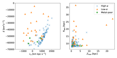
Figure 3: The orbital parameters of the OHS. Different symbols correspond to chemically different subgroups defined in Section 2.2.3 and Figure 4

2.2.3 Chemical abundance subgroups

Figure 4 shows distributions of the OHS in [X/Fe] versus [Fe/H] diagrams. As can be seen, the OHS are widely distributed in [Fe/H] and [X/Fe]. A subset of the stars clearly exhibit relatively low [Mg/Fe] ratios at [Fe/H]$\sim-1.0$, similar to the previously reported low-$\alpha$ population in the solar neighborhood (e.g., Nissen & Schuster, 2010; Ishigaki et al., 2012; Hawkins et al., 2015; Hayes et al., 2018). The large dispersion in [X/Fe] and [Fe/H] among the OHS implies that they have diverse birth environment. We therefore divide the OHS into three subgroups according to the distribution in the [Mg/Fe]-[Fe/H] plane, inspired by preceding studies (e.g., Hawkins et al., 2015; Hayes et al., 2018; Mackereth et al., 2019). The first group is defined as high-[Mg/Fe] stars with [Fe/H]$>-1.5$ (“high-$\alpha$" subgroup; blue crosses in Figure 4). The high-[Mg/Fe] stars with halo-like kinematics are often interpreted as the the early disk populations that have gained high velocity dispersion as a result of minor mergers under the hierarchical Galaxy formation process (e.g., Bonaca et al., 2017; Bonaca et al., 2020; Haywood et al., 2018; Di Matteo et al., 2019; Naidu et al., 2020; Belokurov et al., 2020; Helmi, 2020). As can be seen in Figure 3, these stars are characterized by large $L_{z}$ compared to other stars, which is in line with this interpretation. The second group is defined as low-[Mg/Fe] stars with [Fe/H]$>-1.5$ (“low-$\alpha$" subgroup; orange triangles). As can be seen in Figure 3, the phase-space distribution of the low-$\alpha$ subgroup stars overlap with debris stars of the merger of a single galaxy, known as "Gaia-Enceladus-Sausage" (GES) structure (Belokurov et al., 2018; Helmi et al., 2018, see Section 5.7). The trend of decreasing [Mg/Fe] with increasing [Fe/H] for this subgroup could be attributed to a lower star formation rate in the progenitor galaxy, which has lead to the delayed SN Ia enrichment of Fe significant relative to Mg from CCSNe of massive stars (e.g., Fernández-Alvar et al., 2018). Finally, the OHS includes four stars with [Fe/H]$<-1.5$ (“metal-poor" subgroup; green circles). In general, these stars exhibit a large dispersion in [X/Fe] compared to the two higher-[Fe/H] subgroups. It is beyond the scope of the present work to attribute these stars to the known major identified debris of past accretions (see e.g., Naidu et al., 2020; Aguado et al., 2021; Matsuno et al., 2021)

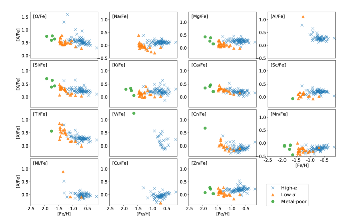
Figure 4: Abundance ratios ([X/Fe]) plotted against [Fe/H] for the three OHS subgroups (“high-$\alpha$", “low-$\alpha$" and “metal-poor") defined in Section 2.2.3.

3 Yield models

3.1 Chemical enrichment scenarios

In this paper, we test four different hypotheses about origin of metals in each of the OHS, which are summarized in Table 1. We describe underlying assumptions and motivations for these hypotheses below.

• Pop III core-collapse supernovae (Model A): In this scenario, similar to Ishigaki et al. (2018), metals are assumed to have predominantly come from a single CCSN of a Pop III stars. Given the relatively high metallicities of the OHS analyzed in this paper, it is an extreme assumption that these stars have formed out of gas purely enriched by a Pop III CCSN. In particular, the high-$\alpha$ OHS subgroup exhibit [Fe/H] as high as $-0.5$, at which this scenario is unlikely even with a tight age constraint as we quantify in Section 5.2.2. These stars, however, may retain a representative enrichment pattern of multiple Pop III CCSNe occurred within a small host halo. For the metal-poor OHS subgroup with [Fe/H]$<-1.5$, a stochastic chemical enrichment in the early Universe coupled with highly inhomogeneous nature of SN metal ejecta would not completely rule out the Pop III CCSNe enrichment (Ritter et al., 2012; Salvadori et al., 2015; Tarumi et al., 2020). By taking into account this scenario, we examine whether the observed patterns of abundance ratios ([X/Fe]) can accept or rule-out the Pop III CCSNe enrichment.

• Pop III $+$ normal core-collapse supernovae (Model B): In this model, we consider a scenario that the ejecta of a Pop III CCSN are mixed with interstellar medium enriched by normal (non-zero-metal) CCSNe. Thus in this scenario, the OHS have formed out of gas enriched by both a Pop III CCSN and normal CCSNe. When the oldest halo stars formed, chemical evolution models generally predict that CCSNe of normal massive stars dominate chemical enrichment. The yields of normal CCSNe depend on both progenitor masses and metallicities (Woosley & Weaver, 1995; Kobayashi et al., 2006; Nomoto et al., 2013). Variation in the characteristic masses or the initial mass function (IMF) of CCSN progenitors is not clearly known, and thus, the Salpeter-type IMF of the form $M^{-\alpha_{\rm IMF}}$ with $\alpha_{\rm IMF}=2.35$ (Salpeter, 1955), which is motivated from local observations, is assumed in this model. Even at the oldest epoch, the metallicity of the normal CCSN progenitors may be different among various Galactic environment with different star formation rates (e.g., Kobayashi et al., 2011). In this scenario (Model B), we fix the IMF to the Salpeter-type IMF, while the metallicities of the normal CCSN progenitors are chosen depending on the observed [Fe/H] of the OHS as detailed in Section 3.3.

• Normal core-collapse supernovae (Model C): In this model, we assume that the elemental abundances of the OHS are predominantly determined by normal CCSNe averaged over an IMF with a characteristic metallicity. In this scenario, the OHS are considered to have formed after the stochastic chemical enrichment by Pop III stars quenched and before the significant metal production by SNe Ia started. In contrast to the Model B, we treat the IMF slope $\alpha$ and $Z_{\rm CC}$ as free parameters within reasonable ranges as detailed in Section 3.3.

• Normal core-collapse $+$ Type Ia supernovae (Model D): In this model, we assume that the metals in the OHS came from both the normal CCSNe and SNe Ia. This scenario is motivated by a speculation that SNe Ia could have contributed to the chemical enrichment in the system even at the oldest epoch when the OHS likely formed. In fact, since progenitor systems of SNe Ia remain controversial, it is not clear when SNe Ia started to contribute to the chemical enrichment in the early Universe at various environments (e.g., Maoz et al., 2014). It has been suggested that there may be a metallicity limit on the occurrence of SNe Ia in single-degenerate systems (Kobayashi et al., 1998; Kobayashi & Nomoto, 2009), but the OHS selected in this paper includes stars with higher metallicities than the limit. In the following analysis, we consider SNe Ia yields of both near-$M_{\rm Ch}$ and sub-$M_{\rm Ch}$ white dwarf progenitors from recent calculations by Leung & Nomoto (2018, 2020), as the origins of metals in the OHS, together with the IMF-averaged normal CCSNe yields. We describe details of the SNe Ia yield models in Section 3.4.

For completeness, we have additionally tested whether a combination of a Pop III CCSN and SNe Ia better explains the observed abundances. We have found that quality of the fit tends to be lower than Models A-D and, in most cases, the maximum possible contribution of SNe Ia is lower than 10 %. We therefore concentrate on Models A-D in this paper. We should note that the Models A-D do not take into account AGB stars as a source of elements detected in the OHS. Galactic chemical evolution models predict that AGB stars are important sources for C, N and neutron-process elements and can contribute after $\sim 30$ Myr after the onset of the Galaxy formation (Kobayashi et al., 2011). For the stars analyzed in this paper, only Y and Ba abundances were reliably measured among the elements likely produced by the AGB stars. We therefore restrict our analysis to elements from O to Zn, for which contributions from AGB stars to the chemical evolution is expected to be small (Kobayashi et al., 2020b). We separately discuss implications from observed Y and Ba abundances in Section 5.6. In the following subsections, we describe the nucleosynthesis yields used in this paper in detail.

Nucleosynthesis source	Model ID	Free parameters	Fixed parameters	Reference
Pop III CCSNe	A	$M$, $E_{51}$, $M_{\rm mix}$, $f_{\rm ej}$, $M_{\rm H}$	-	(1),(2)
Pop III CCSNe $+$ Normal CCSNe	B	$M$, $E_{51}$, $M_{\rm mix}$, $f_{\rm ej}$, $M_{\rm H}$, $f_{\rm CC}$	$\alpha_{\rm IMF}$a, $Z_{\rm CC}$b	(1),(2),(3)
Normal CCSNe	C	$\alpha_{\rm IMF}$, $Z_{\rm CC}$		(3)
Normal CCSNe $+$ SNe Ia	D	$\alpha_{\rm IMF}$, $Z_{\rm CC}$, $f_{\rm Ia}$, $f_{\rm Ch}$c		(3),(4),(5)

Table 1: Description of the four hypothesis (Models A-D) about the origin of metals in the OHS. Reference: (1) Tominaga et al. (2007), (2)Ishigaki et al. (2018), (3)Nomoto et al. (2013), (4)Leung & Nomoto (2018), (5)Leung & Nomoto (2020)

• The IMF slope is fixed at $\alpha_{\rm IMF}=2.35$ for the model B and is changed within $-1\leq\alpha_{\rm IMF}\leq 3$ for the model C.

• The metallicity of CCSNe, $Z_{\rm CC}$, is fixed in Model B according to [Fe/H] of each star (see text for the adopted values). For Models C and D, the value is changed within $0\leq Z_{\rm CC}\leq Z_{\rm obs}$, where $Z_{\rm obs}$ is the metallicity corresponding to [Fe/H] of each star, calculated assuming $Z_{\odot}=0.0152$ (Caffau et al., 2011).

• We tested $f_{\rm Ch}=0.0,0.2,0.5$ and $1.0$.

3.2 Pop III CCSN

We use the same grid of Pop III supernova yield models as has been used to fit the sample of $\sim 200$ EMP stars in I18. The yield models include progenitor masses (13, 15, 25, 40, 100$~{}M_{\odot}$) and explosion energies, $E_{51}=E/10^{51}{\rm[erg]}=0.5$ for the 13$~{}M_{\odot}$ model, 1 for the 13–100$~{}M_{\odot}$ models, 10 for the 25$~{}M_{\odot}$ model, 30 for the $40~{}M_{\odot}$, and 60 for the $100~{}M_{\odot}$ model. The supernova yield models are calculated based on the mixing-fallback model (Umeda & Nomoto, 2002; Tominaga et al., 2007) to approximately take into account mixing among different layers of elements and their fallback to the central compact remnant, which presumably occurs in an aspherical CCSN (Tominaga, 2009). The model employs three parameters, $M_{\rm cut}$, $M_{\rm mix}$, and $f_{\rm ej}$, that correspond to the inner and the outer boundaries of the mixing zone, and the fraction of mass in the mixing zone finally ejected to interstellar medium, respectively. As has been done in I18, we fix $M_{\rm cut}$ at the mass coordinate approximately corresponds to the Fe core radius and vary $M_{\rm mix}$ and $f_{\rm ej}$ as free parameters. For the Model A, we additionally treat hydrogen dilution mass as a free parameter, which is determined to reproduce the observed values of [Fe/H] within a conservative uncertainty of $\pm 0.2$ dex. For the Model B, a total Fe yield is calculated as the sum of Fe yields of a Pop III CCSN and an IMF- and metallicity-averaged normal CCSNe. The mixing-fallback model for the calculation of Pop III CCSN yields have been partly motivated by theoretical predictions that the massive Pop III stars have maintained a high rotational velocity at the end of its evolution (e.g., Ekström et al., 2008) that may affect energy and geometry of the supernova explosion. The yield models used in this work do not self-consistently includes nucleosynthesis specific to rotating massive stars. In reality, it has been suggested that light elements such as N, Na, or Al can be enhanced as a result of rotationally induced mixing during the stellar evolution (e.g., Meynet et al., 2010; Takahashi et al., 2014; Choplin et al., 2019). These elements can also be subject to relatively large uncertainty due to the efficiency of mixing in the stellar interior (e.g., Limongi & Chieffi, 2012). Thus, as in I18, a theoretical uncertainties of 0.5 dex is adopted for Na and Al, which reduces the relative weight of these elements in calculating the quality of the fit. It has been known that the yield models significantly under-predict the yields of Sc, Ti and V (Nomoto et al., 2013), and thus additional nucleosynthesis channels are clearly needed to explain observed abundances of these elements. We therefore treat the model predictions of these abundances as lower limits.

3.3 Normal CCSN

We use the grid of yield models from Kobayashi et al. (2011) and Nomoto et al. (2013), which contains progenitor masses of $13$, $15$, $20$, $25$, and $40M_{\odot}$ with metallicities $Z=0.0,0.001,0.01,0.02$. For each metallicity, we take an average of the yields over the progenitor masses by weighting with an IMF. The IMF of normal CCSN progenitors remain elusive, while available observations have found no significant deviation from the Salpeter-form IMF, $\psi(m)\propto m^{-\alpha_{\rm IMF}}$, with $\alpha_{\rm IMF}=2.35$ (Bastian et al., 2010) for massive stars. For the Model B, we take a linear combination of a Pop III SN and a normal CCSN yield model with an additional parameter $f_{\rm CC}$, which corresponds to the fraction of yield from normal CCSNe relative to the total Pop III SN + normal CCSN yield. The normal CCSN yield is calculated by averaging over a fixed IMF, with a power-low slope of $\alpha_{\rm IMF}=2.35$, and interpolated at the characteristic metallicity, $Z_{\rm CC}$. The value of $Z_{\rm CC}$, is fixed depending on the observed [Fe/H] of the OHS. Specifically, for the metallicities of the CCSN progenitors, we adopt the yields interpolated at $Z_{\rm CC}/Z_{\odot}=0.011$, $0.067$, and $0.209$, for the OHS with [Fe/H]$<-1.2$, $-1.2\leq$[Fe/H]$<-0.7$, and [Fe/H]$\geq-0.7$. These values are compatible with inferred metallicities in bulge, thick disk or halo, for the environments in which old Galactic stellar populations formed (Freeman & Bland-Hawthorn, 2002). For the Model C, in contrast to the Model B, we change $\alpha_{\rm IMF}$ in the range $-1.0\leq\alpha\leq 3.0$ to bracket the values reported by local observations (Bastian et al., 2010). We also treat $Z_{\rm CC}$ as a free parameter in the Model C.

3.4 SN Ia

For the SN Ia yield models, we use the yields of Leung & Nomoto (2018) and Leung & Nomoto (2020) taking into account updates in Kobayashi et al. (2020a), with progenitor metallicities of $Z=0.0$, $0.002$, $0.01$, and $0.02$. Leung & Nomoto (2018) and Leung & Nomoto (2020) provide grids of SN Ia yields for near-Chandrasekhar-mass ($M_{\rm Ch}$) and sub-$M_{\rm Ch}$ white dwarf progenitors, respectively. We make use of the model with a progenitor masses of 1.37$~{}M_{\odot}$ and 1.0$~{}M_{\odot}$, for the near-$M_{\rm Ch}$ and sub-$M_{\rm Ch}$ models, respectively. For the 1.37$~{}M_{\odot}$ white dwarf, we follow Leung & Nomoto (2018), who used this model as the benchmark model of the $M_{\rm Ch}$ white dwarf because it produced the necessary amounts of Mn and Ni matching with the element trends in stars in the solar neighbourhood (see also Kobayashi et al. 2020b). The 1.0$~{}M_{\odot}$ white dwarf is chosen because this model produces $\sim 0.6M_{\odot}$ ⁵⁶Ni in the ejecta, which is the typical amount of ⁵⁶Ni observed in SN Ia (Leung & Nomoto, 2020). For the progenitor metallicities of SN Ia, we assume $Z_{\rm Ia}=0.0$ and $0.1~{}Z_{\odot}$ for the OHS with [Fe/H]$<-1$ and $\geq-1$, respectively. For the Model D, we introduce the parameter, $f_{\rm Ia}$, which corresponds to the number fraction of SNe Ia relative to the total number of normal CCSNe and SNe Ia. In this study, we assume that the number ratio of near-$M_{\rm Ch}$-to-all SN Ia (near-$M_{\rm Ch}$ + sub-$M_{\rm Ch}$) explosions ($f_{\rm Ch}$) to be 0.0, 0.2, 0.5, or 1.0. The value of $f_{\rm Ch}=0.2$ is suggested to reasonably explain the Solar abundance and a local cluster of galaxies by Simionescu et al. (2019). Note that $f_{\rm Ch}\geq 75$ % is suggested from Galactic chemical evolution models (Kobayashi et al., 2020a). The value of $f_{\rm Ch}=1.0$ corresponds to an extreme case where the SNe Ia that have contributed to metals in the OHS all originated from the near-$M_{\rm Ch}$ white dwarf explosions (Leung & Nomoto, 2018).

3.5 Fitting yield models to observed abundances

To fit the yield models to observed abundances, we simply assume that the observed abundances in [X/Fe] are independent and that the likelihood of each [X/Fe] are approximated by a Gaussian function with a standard deviation corresponding to the measurement uncertainty. Although this is a crude assumption, since a true likelihood is unknown and difficult to obtain, we restrict our analysis to this assumption. For the Models A and B, we search for the best-fit yield models that minimize $\chi^{2}$ among the discrete grid of the model parameters as in I18. Under the above assumption, this is equivalent to maximizing the likelihood function. For the Model C and D, where we consider continuous values for the parameter sets, we adopt a Markov-Chain Monte-Carlo (MCMC) algorithm to sample posterior probability distributions of the parameters. For this purpose, we make use of PyMC3 (Salvatier et al., 2016) adopting flat priors for all the fitting parameters in the range described in Table 1.

4 Results

In the following subsections, we describe results of fitting the parameters of Models A–D to the observed chemical abundances in the OHS sample. The estimated model parameters for all the OHS are given in Tables 2-5

4.1 Pop III CCSN yields (Model A)

The left panels of Figure 5 show the best-fit Pop III CCSN yield model and observed abundances for representative stars from the three OHS subgroups. The top panel is for one of the high-$\alpha$ OHS, whose abundance pattern is characterized by small odd-even elemental abundance ratios among Na - Ca. Among the yield models considered, this pattern is best explained by the Pop III CCSN yield with a progenitor mass of 15$M_{\odot}$. The middle panel shows the best-fit model for one of the low-$\alpha$ OHS. The low [Mg/Fe] of this star is reproduced by the 25$M_{\odot}$ Pop III CCSN yield model. The bottom panel shows the best-fit model for one of the metal-poor OHS. The high [O/Fe] and [Si/Fe] ratios in this star are reproduced by the 40$M_{\odot}$ Pop III CCSN yield model. For all the best-fit models, the abundance ratios of odd-Z elements such as Mn are under-produced, implying a need for additional metal-enrichment sources for this element. The best-fit Pop III CCSN progenitor masses for the three OHS subgroups are summarized in the left panel of Figure 6. Overall, the observed abundance patterns of the OHS are predominantly explained by Pop III CCSN progenitor models of either 15 or 25 $M_{\odot}$. A large fraction of the high-$\alpha$ subgroup is best fitted by the $15M_{\odot}$ model, while the low-$\alpha$ or metal-poor subgroups are better explained by the 25$M_{\odot}$ model. The ejected masses of a radio-active ⁵⁶Ni isotope, which decays to ⁵⁶Fe, is $\sim 10^{-2}-10^{-1}M_{\odot}$ for the majority of the best-fit Pop-III CCSN yield models. To explain observed [Fe/H] values of the OHS by a single Pop III yield that fits the abundances, the ejected Fe should be diluted with only $10^{2}-10^{3}M_{\odot}$ of hydrogen in most cases (Table 2). These values are extremely small compared to simulations of metal mixing and analytical models (Magg et al., 2020). We discuss the validity of this scenario in Section 5.2.

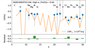
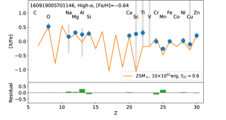
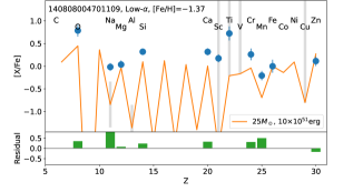
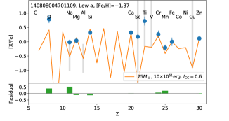
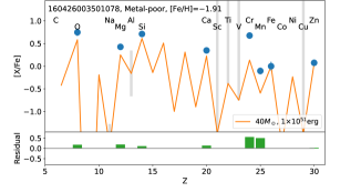
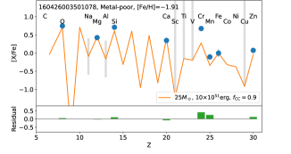
Figure 5: The best-fit yield models (Model A: left and Model B: right) compared with observed abundances for the representative stars from the three OHS subgroups. From top to bottom, the result for the representative star from the high-$\alpha$, low-$\alpha$ and metal-poor subgroups are shown with GALAH ID, subgroup status and [Fe/H] at the top-left. In each panel, the solid line shows the best-fit yield model, where the corresponding parameter values are shown at the bottom-right. The filled circles correspond to the observed abundances from GALAH DR3. The gray vertical bars mark the elements for which a large theoretical uncertainty is assumed (Na and Al) or the model values are treated as lower limits (Sc, Ti, V, and Cu). The residuals are shown by solid bars at the bottom of each panel.

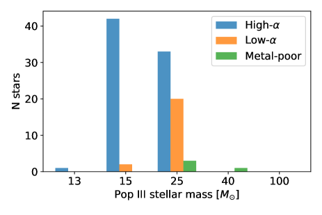
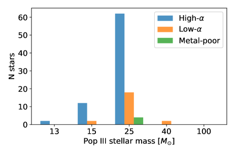
Figure 6: The best-fit Pop III stellar masses (13, 15, 25, 40 or 100$M_{\odot}$) for the Models A(left) and B (right). The results from the three OHS subgroups are shown by different colors.

4.2 Pop III and CCSNe yields (Model B)

The right panels of Figure 5 show the best-fit Pop III + CCSN yield models (Model B) and the observed abundances for the same representative stars from the three OHS subgroups as in the left panels. Compared to the Model A results, quality of the fits to the O, Na, Mg, and Al abundance ratios improve as a result of considering the additional contribution from normal CCSNe. In each panel, the best-fit fraction of normal CCSNe are indicated in the bottom-left corner. The metal-poor OHS tends to be better fitted by larger fraction of normal CCSNe relative to Pop III SNe. This is partly resulted from the low metallicity of the normal CCSNe assumed for the metal-poor OHS with [Fe/H]$<-1.5$. The results of the best-fit Pop III stellar masses are shown in the right panel of Figure 6. Taking into account the contamination from normal CCSNe, the majority of the OHS are best fitted by the 25$M_{\odot}$ Pop III CCSN yield models that produce $\sim 10^{-1}M_{\odot}$ of ⁵⁶Fe (Table 3). Similar to Model A, however, the Fe yields from Pop III CCSN that best explain observed abundances violate the constraint on the amount of diluting hydrogen gas to be compatible with the observed [Fe/H] (Magg et al., 2020). We discuss the validity of the Models A and B in Section 5.2.

4.3 Normal CCSN yields (Model C)

Figure 7 shows results of fitting normal CCSN yields with the IMF slope ($\alpha_{\rm IMF}$) and the characteristic metallicity of CCSN ($Z_{\rm CC}$) for the representative stars from three OHS subgroups. The resulting parameter estimates for all the OHS are summarized in Figure 8 and in Table 4. To illustrate how the predicted abundances change with $\alpha_{\rm IMF}$, the left panels of Figure 7 show the yield models corresponding to the minimum and the maximum values that bracket the 94% highest density interval (HDI) of the posterior distribution of $\alpha_{\rm IMF}$, where the HDI provides a measure of uncertainty in the parameter estimate. The mean $\alpha_{\rm IMF}$ value from the posterior distribution is very close to the maximum allowed value for $\alpha_{\rm IMF}$ we have taken into account. The models with smaller $\alpha_{\rm IMF}$ predict [X/Fe] of elements from O-Si significantly higher than the observed abundances. The larger $\alpha_{\rm IMF}$ corresponds to the larger contribution from less massive stars. The results thus suggest that, in the context of Model C, the OHS are better explained by a larger contribution from lower-mass CCSN progenitor stars than expected from the Salpeter IMF with the slope of $-2.35$. Similar to the left panels, the right panels of Figure 7 illustrate the change in the model abundances with $Z_{\rm CC}$. The dashed and dotted lines indicate the models corresponding to the lower and higher bounds of the 94% HDI of the posterior distribution of $Z_{\rm CC}$. The change in predicted patterns among different $Z_{\rm CC}$ is small for the measured elemental abundance ratios. As can be seen in Figure 8, for most of the OHS, the mean values of $Z_{\rm CC}$ are close to the observed metallicity of the OHS (dotted lines).

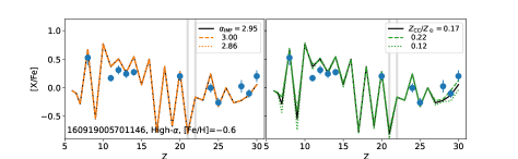
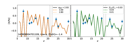
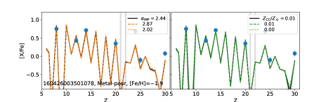
Figure 7: The abundance patterns of IMF-averaged normal CCSN yield models (Model C) compared with observed abundances. In each panel, the solid line shows the model with the parameters corresponding to the mean of the posterior probability distribution. The circles with error bars are the abundances from the GALAH DR3. The left and right panels show the changes in the model abundance pattern by changing $\alpha_{\rm IMF}$ and $Z_{\rm CC}$, respectively. In each panel, the dashed and dotted lines correspond to the lower and higher bounds of the 94 % highest density interval of the posterior probability distribution. The gray vertical bands indicate the elements that are not taken into account in the fitting.

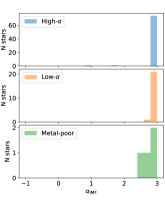
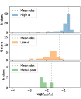
Figure 8: Mean values of the posterior probability distributions for the model parameters, $\alpha_{\rm IMF}$ (left) and $Z_{\rm CC}$ (right) obtained by the MCMC sampling. The histograms for the three subgroups are shown from top to bottom. In the right panels, the vertical lines correspond to mean metallicities of the observed stars in each subgroup.

4.4 Normal CCSN and SN Ia yields (Model D)

Finally, results of fitting yield models of normal CCSNe combined with SNe Ia are shown in Figure 9 for the representative stars of the three OHS subgroups. The result for the case of $f_{\rm Ch}=0.5$ (equal contributions from near-$M_{\rm Ch}$ and sub-$M_{\rm Ch}$ SN Ia progenitors) is shown. The results for all the OHS are given in Table 5. Figure 9 shows abundance patterns corresponding to the mean values of the posterior probability distribution of the model parameters. To illustrate the parameter dependence of the model prediction, different columns show the models with different values of the IMF slope of the CCSN progenitors ($\alpha_{\rm IMF}$; left), characteristic metallicity of the CCSNe ($Z_{\rm CC}$; middle) and the SN Ia fraction ($f_{\rm Ia}$; right). Compared to the CCSN-only model (Model C, Figure 7), the observed abundance ratios are much better reproduced, especially for the high-$\alpha$ and the low-$\alpha$ OHS subgroups. Mean parameter values for $\alpha_{\rm IMF}$, $Z_{\rm CC}$ and $f_{\rm Ia}$ from the posterior distributions for each OHS subgroup are summarized in Figure 10 for the case of $f_{\rm Ch}=0.5$. Similar to the result of Model C, the left panel shows that $\alpha_{\rm IMF}$ are mostly distributed around the steepest possible slope, $\alpha_{\rm IMF}=3.0$, we have taken into account. The values of $Z_{\rm CC}$ are in the range 0.03-0.27$Z_{\odot}$, which are close to the metallicity of the OHS themselves (dotted vertical lines). The right panel of Figure 10 shows that the values of $f_{\rm Ia}$ for the high-$\alpha$ subgroup range from 0.00 up to 0.20 (0.08 on average). The $f_{\rm Ia}$ values are, on average, higher for the low-$\alpha$ subgroup (0.01-0.27, 0.09 on average). For the metal-poor subgroup, the $f_{\rm Ia}$ values are at most $\sim 0.05$, which are lower than the other two subgroups. The SN Ia fractions depend on the different assumptions about $f_{\rm Ch}$. If $f_{\rm Ch}=1.0$ (all SNe Ia from near-$M_{\rm Ch}$ progenitors), instead of $f_{\rm Ch}=0.5$, is assumed, the SN Ia fractions slightly decrease by a few percent for all of the OHS subgroups. To compare the models with different values of $f_{\rm Ch}$ and with the normal CCSNe only model (Model C), for each OHS, we obtain a ranking of these models according to the quality of the fit by penalizing with the number of parameters. Figure 11 summarizes the number of stars that are best explained by the models with $f_{\rm Ch}=0.0$, $0.2$, $0.5$ or $1.0$ or with the normal CCSN only. For the high-$\alpha$ and low-$\alpha$ OHS, we find that the model with $f_{\rm Ch}=0.5$ most frequently best explains the observed abundances. On the other hand, for the metal-poor OHS, the model with $f_{\rm Ch}=1.0$ more frequently best explains the observed abundances.

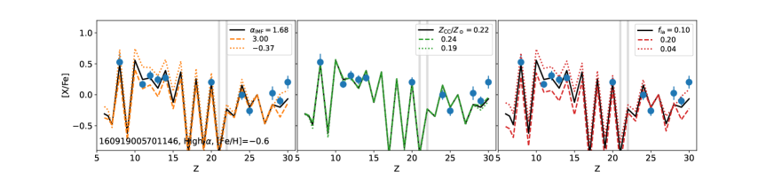
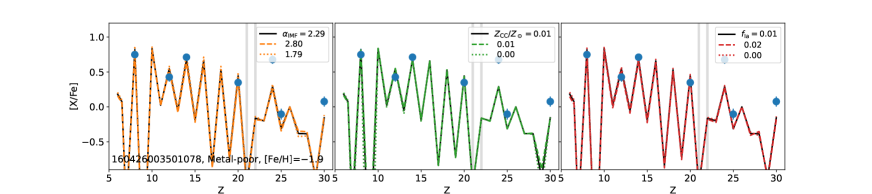
Figure 9: The abundance ratios ([X/Fe]) of the best-fit yield models that assume contributions from both the IMF-averaged normal CCSNe and SNe Ia (Model D). The stars are sorted in order of their metallicity (decreasing from top to bottom). The case for $f_{\rm Ch}=0.5$ is shown. In each panel, the solid line shows the best-fit models and the circles with error bars are the abundances from the GALAH DR2. The models with changing the model parameters, $\alpha$, $Z_{\rm CC}$ and $f_{\rm Ia}$, are shown in the left, middle and right columns, respectively. The gray vertical bands indicate the elements that are not taken into account in the fitting.

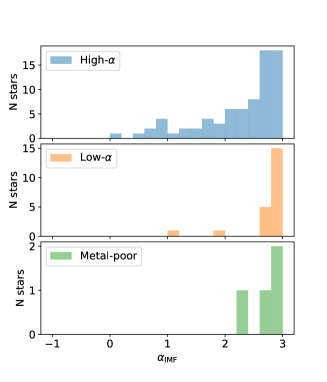
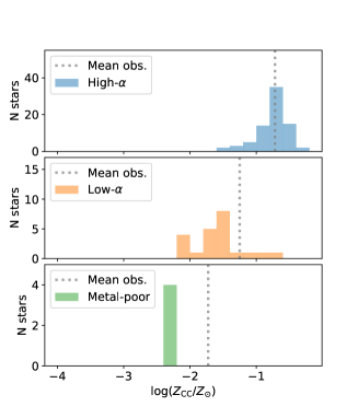
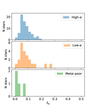
Figure 10: Mean values of the posterior probability distributions for the model parameters, $\alpha_{\rm IMF}$ (left), $Z_{\rm CC}$ (middle) and $f_{\rm Ia}$ (right) obtained by the MCMC sampling. The histograms for the three subgroups are shown from top to bottom. The case for $f_{\rm Ch}=0.5$ is shown. In the middle panels, the vertical lines correspond to mean metallicities of the observed stars in each subgroup.

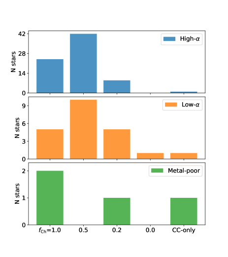
Figure 11: The number of stars that are best explained by Model D with $f_{\rm Ch}=1.0,0.5,0.2$ or $0.0$ (the four bars on the left) or by Model C (the bars on the right).

5 Discussion

Identifying nucleosynthetic sources at various galactic environments in the early Universe remains a major challenge in studies of the cosmic chemical evolution, since it is not feasible to directly observe individual stars or SN events at high redshifts. In our study, we address this question by elemental abundances measured by GALAH DR3 (Buder et al., 2021) for relatively old Milky Way halo stars (“OHS”)) in the solar neighborhood. We have considered yield models that represent four different hypotheses about the origin of metals in the atmosphere of the OHS (Models A-D). For each of the Models A-D, we have obtained the model parameters that reproduce observed elemental abundances.

5.1 Comparison among models

Figure 12 summarizes the best-fit model obtained for each of the Models A-D compared to the observed abundances for the representative stars of the three OHS subgroups. For both the high-$\alpha$ and low-$\alpha$ OHS shown in the top two panels of Figure 12, either the Pop III + normal CCSNe (Model B; dotted line) or the normal CCSNe + SN Ia (Model D; solid line) yields provide a better fit than the other two models. The Pop III CCSN model (Model A; dashed line) tends to significantly under-predict the abundance ratios of odd-atomic-numbered elements such as Al, or Cu. The normal CCSN model (Model C; dash-dotted line) over-predict the observed abundance ratios of elements from O to Si. In the case of the metal-poor OHS shown in the bottom panel, the difference among the best-fit Models B-D is small since the yields of normal CCSN with low metallicity dominate over the Pop III CCSNe or SN Ia. We note that a quantitative comparison among Models A-D is not straightforward because the four models employ different numbers of model parameters, which are not nessesarily independent. Therefore, the comparison of the reduced $\chi 2$ values between different models should be viewed with caution. In the next subsections, we discuss validity of each model in terms of other constraints from simulations and observations.

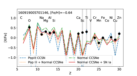
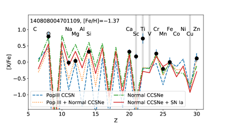
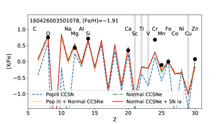
Figure 12: Summary of the best-fit models obtained for the Models A (dashed line), B (dotted line), C (dash-dotted line) and D (solid liinie) for the representative stars of the three OHS subgroups. The observed abundances are shown in black circles.

5.2 Pop III CCSNe

Cosmological simulations including metal enrichment by early generations of massive stars generally predict that the metal pollution is patchy and thus pristine gas for the formation of Pop III stars can survive over a wide range of cosmic time (e.g. Maio et al., 2010). With cosmological hydrodynamical simulations over a volume of $(10{\rm~{}Mpc}h^{-1})^{3}$, Pallottini et al. (2014) suggest that the formation of Pop III stars from pristine gas can occur at least up to $z=4$ in regions far from star-forming galaxies and in low mass halos ($M_{\rm h}\lesssim~{}10^{8}M_{\odot}$). In the following we examine the validity of the Pop III CCSN enrichment scenario in terms of best-fit Pop III CCSN models obtained in the previous section (Section 4.1) and in terms of semi-analytical models for chemical enrichment in the context of the hierarchical galaxy formation scenario (Section 5.2.2).

5.2.1 Best-fit Pop III CCSN model parameters

If the OHS are actually very old stars (e.g., $>12$ Gyrs), they could potentially be the first metal-enriched stars formed out of gas locally pre-enriched by Pop III stars. As the result of comparing observed abundances with the Pop III CCSN yield models, we find that the abundance patterns of the OHS are best explained by the Pop III stars with progenitor masses of 15 or 25 $M_{\odot}$. One difficulty of the Model A is that the ISM from which the OHS have formed should have been pre-enriched with neutron capture elements, such as Y or Ba, both detected in the OHS. These elements are synthesized by both rapid (r-) and slow (s-) neutron capture processes, which generally require Fe seed nuclei. These processes, therefore, are not likely associated with Pop III stars with strictly zero metal content (see Choplin et al. 2020 for a possible channel to produce neutron-capture elements in a low-metallicity massive star). The abundances of the [Ba/H] and [Y/H] in the OHS are a several orders of magnitudes higher than typical EMP stars and an order of magnitude higher than the values observed in the r-rich ultra-faint dwarf galaxy (e.g., Ji et al., 2016). Moreover, since the [Ba/Y] ratio of the OHS are close to the solar value, both r- and s- process should have contributed unlike the pure r-process ratios reported by Ji et al. (2016). Another potential difficulty of the scenario is that the required mass of hydrogen to dilute ejected Fe to be compatible with the observed [Fe/H] value is extremely small. With an analytic prescription (e.g., Thornton et al., 1998; Tominaga et al., 2007), the swept up hydrogen mass by ejecta of a supernova with a given explosion energy of $E_{51}=1$ is estimated to be 10${}^{5}~{}M_{\odot}$ for the hydrogen number density, n=1–100 cm^-3. In contrast, the hydrogen dilution mass required to explain both [X/Fe] ratios and [Fe/H] is determined to be 100–1000$~{}M_{\odot}$, which is much smaller than the analytic prescription. This value is also not compatible with a new estimate of the minimum dilution mass by Magg et al. (2020). In those respect, it is unlikely that only a single Pop III supernova dominate in producing metals in the OHS. In order to more robustly conclude on the possible chemical signature of Pop III stars in the OHS, theoretical investigations on the possible distributions of metallicity of the first metal-enriched stars are nessesary (Karlsson et al., 2013; Smith et al., 2015). It has been proposed that various different mechanisms could have played a role in determining the condition at which the first metal-enriched stars form, potentially leading to the [Fe/H] spread. They includes (1) the properties of the Pop III stellar systems such as the IMF, multiplicity, and the number of Pop III stars per mini halos (Clark et al., 2011; Greif et al., 2011; Stacy & Bromm, 2014; Susa et al., 2014; Hartwig et al., 2018), (2) hydrodynamical properties of Pop III SN ejecta that could depend on the explosion energy and geometry (Joggerst et al., 2009; Tominaga, 2009; Ritter et al., 2012), (3) the properties of the interstellar medium to which energy and metals from Pop III SNe are injected (Kitayama & Yoshida, 2005; Greif et al., 2010; Jeon et al., 2014; Chiaki et al., 2018; Tarumi et al., 2020), (4) metals and dust abundances that determine the efficiency of the formation of the next-generation low-mass stars (e.g., Omukai et al., 2005; Chiaki et al., 2014; de Bennassuti et al., 2014; Hartwig & Yoshida, 2019) and (5) the redshift evolution of CMB and the properties of the host halos (Tumlinson, 2007; Smith et al., 2009). Predictions on their combined effects on the [Fe/H] spread among the first metal-enriched stars would provide useful insights into the best strategy for the upcoming Galactic Archaeology surveys.

5.2.2 Can stellar ages help to select stars purely enriched by Pop III stars?

Based on the paradigm of hierarchical structure formation and incremental chemical enrichment over comic time, we expect a causal connection between the age and chemical composition of a star. Our finding of several old stars at [Fe/H]$>-1$, with abundance ratios similar to Pop III CCSN yield models raises the question if we can use this insight to select interesting candidates for stellar archaeology based on an age selection. To answer these questions, we use the semi-analytical model a-sloth (Ancient Stars and Local Observables by Tracing Haloes) based on Hartwig et al. (2018) and Magg et al. in prep. with an improved subgrid model for stochastic metal mixing in the first galaxies (Tarumi et al., 2020). More technical details of a sloth can be found in the corresponding references, and we briefly summarize its main features here. On top of 30 Milky Way-like dark matter merger trees from the Caterpillar simulation (Griffen et al., 2016), we model Pop III star formation by following chemical, radiative, and mechanical feedback. This allows us to analyse the chemical enrichment history of the Milky Way with detailed abundance and age information of stars that end up in the Milky Way halo at $z=0$. In our fiducial model (calibrated against the metallicity distribution function, see Tarumi et al., 2020), we use a Pop III IMF from 2-180 M_⊙ with a slope of $\mathrm{d}N/\mathrm{d}M=-0.5$, and a Pop III star formation efficiency of $1\%$. With this model, we can predict what fraction of metals in a star comes from Pop III SNe or from later generations of stars. The results as a function of metallicity are illustrated in Figure 13.

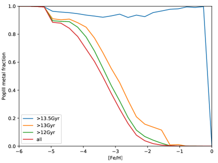
Figure 13: Simulated fraction of metals in MW stars that come from Pop III SNe as a function of stellar metallicities. The different lines illustrate how an age cut helps to select interesting candidates that are dominated by metals from Pop III SNe. A theoretical age selection of $>13.5$ Gyr could help to select such Pop III-dominated stars at metallicities up to [Fe/H]$\sim 0$.

The overall trend for all stars (red line) shows that the average fraction of metals from Pop III SNe decreases monotonically with metallicity. The contribution of metals from Pop III SNe to stars with [Fe/H]$>-2$ is only $<10\%$. The semi-analytical model predicts that metals from Pop III stars are insignificant for the OHS with [Fe/H]$>-1$. However, if we could select old stars with $>13.5$ Gyr, this picture changes dramatically. The metal content of such old stars is dominated ($>80\%$) by Pop III SNe at all metallicities up to solar. Although challenging in reality, such an age pre-selection could be very valuable to pre-select interesting candidates for stellar archaeology at [Fe/H]$>-3$. This plot also shows another property of general interest: the fractional Pop III contribution as a function of metallicity. For EMP stars ([Fe/H]$<-3$), at least $50\%$ of their metal mass comes from Pop III SNe. This value increases to $\gtrsim 80\%$ at [Fe/H]$<-4$. Another interesting related question is if we can identify mono-enriched stars at higher metallicities with the help of an age selection. We show the mono-enriched fraction as a function of metallicity in Figure 14.

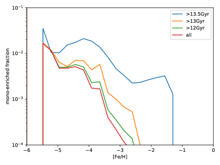
Figure 14: Fraction of stars that are enriched by only one Pop III SN as a function of metallicity. The lines represent different age cuts, which may allow to pre-select interesting candidates. While an age-cut increases the fraction of mono-enriched stars at all metallicities, there are no mono-enriched stars at [Fe/H]$>-1$ in our model.

An age-cut can help to increase the fraction of mono-enriched stars in the sample, but the requirements of age precision are beyond current isochrone-based estimates. Moreover, the overall numbers of mono-enrichment depend strongly on the assumed Pop III star formation efficiency, which is only weakly constrained. In summary, and age-cut is a valuable tool to select interesting, informative candidates for stellar archaeology, but the precision of the age estimate needs to be improved for this method to be reliable.

5.3 Pop III and Normal CCSNe

We next discuss whether the observed abundances in the OHS imply the scenario that both Pop III and normal CCSNe contribute to the metal enrichment (Model B). In what condition this scenario is realized is not clear because of the complexity in physical mechanisms that determine the degree of homogeneity in star forming environment in the early Universe. A motivation of this scenario is that, at redshift $z>3$, when a sizable fraction of Milky Way halo stars formed, it may be possible that, the systems is mainly chemically enriched by normal CCSNe, while there is remaining pristine gas, which could form Pop III CCSN progenitors. We have found that, the contributions from both Pop III and normal CCSNe reasonably well explain observed elemental abundances in the OHS. The combined yields simultaneously explain the abundance ratios for both the intermediate-mass elements (Na-Si) and the iron-peak elements (Cr-Zn) (right panels of Figure 5). Similar to the Model A, nearly solar [Y/Fe], and [Ba/Fe] ratios in the OHS remain difficult to explain, which requires a pre-enrichment of both r- and s-process elements to the ISM prior to the Pop III CCSN. Validity of this scenario is, therefore, depends on the possible sources of the neutron-capture elements in the cosmic epoch when Pop III stars was still contributing to the chemical enrichment.

5.4 Normal CCSNe

Under the assumption that yields of normal CCSNe dominate the metal abundances in the OHS (Model C), none of the yield models we have taken into account explain the data better than the other three models. For the high-$\alpha$ and low-$\alpha$ OHS with [Fe/H]$>-1.5$, the predicted abundance patterns of elements from O to Si relative to Fe are much higher than observed values unless unusually steep IMF slopes such as $\alpha_{\rm IMF}>3$ are assumed. This result is robust against change in the progenitor metallicity ($Z_{\rm CC}$). We therefore conclude that the yields of normal CCSNe alone is not likely as the origin of the metal abundances in the OHS, unless the IMF is extremely bottom heavy. Observations of high-redshift galaxies or different Galactic regions have reported a possible signature of variations in the IMF with cosmic time or with local environment (Bastian et al., 2010). In particular, recent studies have provided evidences that the IMF is top-heavy for environments with high star formation rates (Cowley et al., 2019, and reference therein). The values of $\alpha_{\rm IMF}$ to better explain the OHS’s abundances, on the other hand, imply a significantly steeper or a bottom-heavy IMF for the normal CCSN progenitors, which is not motivated by any other observations (Bastian et al., 2010).

5.5 SNe Ia

The cumulative contribution of SNe Ia to metals in the present Universe has been studied through the Solar chemical composition (e.g., Tsujimoto et al., 1995) or the abundances in the intra-cluster medium (ICM) in nearby clusters of galaxies (Matsushita et al., 2003; de Plaa et al., 2007; Simionescu et al., 2015; Mernier et al., 2016). In one of the latest studies on this topic, Simionescu et al. (2019) employed recent CCSN and SN Ia yield calculations to explain the observed abundance ratios 11 different chemical elements detected in the core of the Perseus cluster of galaxies from high-resolution X-ray spectroscopy. Depending on the yield models used, they find that 13–40 % of SNe that have contributed to the metal enrichment are SN Ia and that 9–36 % of all SNe Ia are associated with near-$M_{\rm Ch}$ progenitors. How the SN Ia rate changes as a function of cosmic time or of environments remains elusive because there is no consensus about the progenitor systems and the mechanisms which make the system to finally explode. The observed lack of evolution of the Fe content in the ICM of clusters of galaxies out to redshift $\sim 2$ (McDonald et al., 2016; Mantz et al., 2017; Liu et al., 2020; Mantz et al., 2020) suggests that metal enrichment by SN Ia was already important early during cosmic history. This is further confirmed by measurements of the metal abundances in the outskirts of nearby galaxy clusters (Werner et al., 2013; Urban et al., 2017); the remarkably uniform distribution of Fe over large spatial scales, and the small cluster-to-cluster scatter, suggest that the ICM was enriched more than 10 billion years ago, before these clusters developed a strongly stratified entropy gradient that would prevent the efficient mixing of metals. The SN Ia rate evolution at high redshifts has also been addressed through the characteristic delay time or the delay time distribution for SN Ia (e.g., Hopkins & Beacom, 2006; Totani et al., 2008; Hachisu et al., 2008; Maoz et al., 2014). Based on the observed cosmic star formation rate density evolution, Hopkins & Beacom (2006) suggest a characteristic delay time of $t\sim 3$ Gyrs, with no strong evidence of a “prompt” component (i.e., no time delay). On the other hand, other studies suggest that SN Ia can explode sooner after a starburst event. Totani et al. (2008) have found that a delay time distribution of the form $\propto t^{-1}$ at delays $>1$ Gyrs best explains their observations of SN Ia rates for a sample of elliptical galaxies, which is generally consistent with the DD scenario (see, however, Hachisu et al. 2008 for the explanation of the $t^{-1}$ delay time distribution with the SD scenario). Maoz et al. (2012) find a continuous delay time distribution, with significant detections of prompt ($<0.4$ Gyr), intermediate ($0.4-2.4$ Gyr), and delayed ($>2.4$ Gyr) explosions. If the ages of the OHS are accurately greater than 12 Gyrs, they provide additional insights into the SN Ia rates at high redshifts. Fitting the abundance ratios of $\alpha$ and Fe-peak elements simultaneously helps alleviating the degeneracy between the SN Ia fraction and the IMF slope of CCSN progenitors. We find that the model in which 4-6% of all the metal-enriching SNe are SN Ia best explains the abundances of the OHS with [Fe/H]$>-1.5$. The smaller relative SN Ia contribution requires the IMF of the CCSN progenitors to be unusually steep ($>3$). The Type Ia supernovae are so far the only channel for synthesizing Mn consistent with the solar composition (Seitenzahl et al., 2013; Nomoto & Leung, 2017b). The observed [Mn/Fe] ratios in the OHS, therefore, provide strong hints on the previous contamination by SNe Ia. Although the SN Ia enrichment in the first few billion years of the Universe remains elusive (Maoz et al., 2014; Hopkins & Beacom, 2006), the results presented here are in line with the early chemical enrichment inferred from metal abundance distributions in nearby and high-redshift galaxy clusters (e.g., Mantz et al., 2020). It is, however, not well established whether near-$M_{\rm Ch}$ white dwarfs or sub-$M_{\rm Ch}$ white dwarfs are the dominant SNe Ia progenitors at high redshifts. The ICM abundances in galaxy clusters hint at a certain contribution from sub-$M_{\rm Ch}$ SN Ia enrichments (Simionescu et al., 2019). Chemical abundance ratios in the stars of ancient dwarf Milky Way satellite galaxies also support contributions of sub-$M_{\rm Ch}$ SN Ia (Kirby et al., 2019; Kobayashi et al., 2020a).

5.6 Contributions from other sources

In this section we discuss the abundances of elements that are potentially affected by nucleosynthetic sources other than Pop III/normal CCSNe or SN Ia.

5.6.1 Y and Ba

For the solar system material, more than 80 % of Y and Ba are attributed to main s-process in AGB stars (Arlandini et al., 1999; Prantzos et al., 2020). In the early Galaxy, stellar winds from fast-rotating massive stars (Meynet et al., 2006; Hirschi, 2007; Ekström et al., 2008; Yoon et al., 2012) are predicted to have significant contribution to the metal enrichment, including s-process elements like Y or Ba (Pignatari et al., 2008; Chiappini et al., 2011; Frischknecht et al., 2016; Choplin et al., 2018; Limongi & Chieffi, 2018; Prantzos et al., 2018). In addition, Ba is likely synthesized by the main $r$-process in the early Universe, whose major astrophysical site is subject to debate (e.g., Cowan et al., 2019). In addition to the main $r$-process, other sources are required for the production of Y to be compatible with observed abundance patterns in EMP stars (e.g., François et al., 2007). Figure 15 shows the [Y/Fe] and [Ba/Fe] abundance ratios for the three OHS subgroups. The low-$\alpha$ OHS show lower [Y/Fe] than the high-alpha OHS at [Fe/H]$\sim-1$ as reported by preceding studies (Ishigaki et al., 2013; Fishlock et al., 2017; Matsuno et al., 2020). On the contrary, the [Ba/Fe] ratios of the low-$\alpha$ OHS are indistinguishable from the high-$\alpha$ OHS. The metal-poor OHS subgroup is characterized by large scatter in both the [Y/Fe] and [Ba/Fe] ratios. The diversity of these neutron-capture elemental abundances hints at the environmental dependence in the s-process enrichment among the oldest nearby halo stars. In order to clarify which of the proposed sites are responsible for producing each of Y and Ba in the OHS, abundance determinations of C and N as well as other neutron-capture elements are necessary.

5.6.2 Zn

Another sources, that could have contributed to the observed abundances in OHS are nucleosynthetic products of stars with masses $\sim 8-10~{}M_{\odot}$, which end their life as electron-capture supernovae (Nomoto, 1984, 1987). Electron capture supernovae are triggered by electron capture on ²⁰Ne when the mass of the electron-degenerate O-Ne-Mg core of $\sim 8-10~{}M_{\odot}$ stars becomes near the Chandrasekhar mass limit ($\sim 1.4M_{\odot}$) so that the central density gets close to the threshold density (Nomoto, 1984, 1987; Nomoto & Leung, 2017a; Leung & Nomoto, 2019; Jones et al., 2019). The contribution to GCE models are thought to be negligible, except for neutron-capture elements (Kobayashi et al., 2020b). The evolution of the progenitor with O-Ne-Mg core based on most recent microphysics model (Suzuki et al., 2019) suggest that electron-capture supernova is triggered at the central density of log $\rho_{c}$(g cm${}^{-3})>10.01$ in the majority of parameter space on convection, etc., which is very likely to lead to collapse to form neutron stars (Zha et al., 2019; Leung et al., 2020). An alternative channel for synthesizing matter with a high Zn/Fe ratio is the collapsar (Tsuruta et al., 2018). The high velocity jet triggered by the central rotating black hole formed by the core in a massive star provides the necessary shock heating. The thermal energy creates the necessary high entropy zone during the alpha-rich freezeout burning (Maeda et al., 2002; Matsuba et al., 2004). To test whether the possible contribution of Zn other than CCSNe or SN Ia could affect our conclusion on the relative CCSNe and SNIa fractions, we repeat the fitting for the Model D with $f_{\rm Ch}=1.0$, considering the model abundance of Zn as a lower limit. The results on the best-fit model parameters do not change significantly, since all the models shown in Fig 9 under-predict [Zn/Fe]. This indicates that the possible contribution from additional Zn sources does not affect the main conclusion in the present analysis.

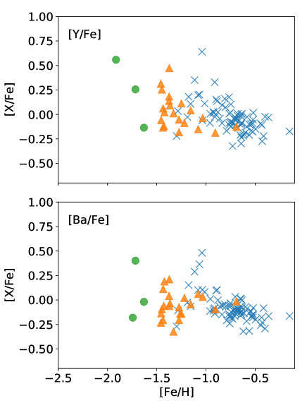
Figure 15: [Y/Fe] and [Ba/Fe] ratios of the three OHS subgroups. Symbols are the same as in Figure 4.

5.7 Relation to known Galactic stellar populations

The OHS analyzed in this study have been selected to have orbital kinematics compatible with the stellar halo population of the Galaxy (Section 2.2.2). The origin of the stellar halo has been debated for many decades (e.g., Eggen et al., 1962; Searle & Zinn, 1978; Chiba & Beers, 2000; Carollo et al., 2007), and it is still being actively discussed (e.g., Helmi, 2020). In particular, astrometric data from Gaia combined with ground-based massive photometric and spectroscopic surveys have made a major breakthrough in this discussion by the discovery of a clear evidence of a merger at the early Galactic formation epoch ($z\sim 1-2$) (e.g., Belokurov et al., 2018; Helmi et al., 2018). The debris stars of this merger event, called “Gaia-Enceladus-Sausage (GES)”, are found to constitute a large fraction of the local stellar halo population (e.g., Di Matteo et al., 2019; Naidu et al., 2020). The discovery of GES is in line with the hierarchical formation of the Galaxy as predicted by cosmological simulations (Bullock & Johnston, 2005; Font et al., 2006; De Lucia & Helmi, 2008; Cooper et al., 2010). The majority of remaining local halo stars are found to be on prograde orbits and have metallicities similar to the thick disk population (Haywood et al., 2018; Di Matteo et al., 2019; Bonaca et al., 2020; Belokurov et al., 2020). These characteristic kinematics and metallicities are compatible with the population formed in-situ, presumably in the old disk or bulge, part of which have dynamically heated by accretion events (Zolotov et al., 2010; Purcell et al., 2010; Tissera et al., 2013). The dynamical heating is thought to be largely associated with the GES merger event, which is predicted to have occurred 8-10 Gyrs ago (Helmi et al., 2018; Mackereth et al., 2019; Gallart et al., 2019; Belokurov et al., 2020; Grand et al., 2020). The OHS provides a unique opportunity to observationally constrain the early Galactic environment, prior to the merger of GES, thanks to the detailed elemental abundance measurements from the GALAH catalogs (see also Fernández-Alvar et al., 2018). The high-$\alpha$ OHS includes stars with [Fe/H] as high as $\sim-0.3$. We have shown that, regardless of the assumptions about the IMF of normal CCSN progenitors, the observed abundances of the high-$\alpha$ OHS are best explained by yields of the normal CCSNe with metallicities as high as $Z_{\rm cc}/Z_{\odot}\sim 0.1-0.3$, suggesting that the enrichment by the normal CCSNe should have been very efficient and have occurred on short timescales. At the same time, the observed abundances of the high-$\alpha$ OHS are better explained with a certain (up to 10 %) contribution of SN Ia. This implies that SN Ia, which produce $\sim 10$ times more Fe than a normal CCSN, have played a role in the chemical enrichment in the earliest epoch of the Galaxy formation. The low-$\alpha$ OHS with [Fe/H] in the range from $-1.5$ up to $-0.7$ includes stars showing a sign of larger contribution from SN Ia (up to 20 %). On the other hand, the metal-poor OHS with [Fe/H]$<-1.5$ do not exhibit strong evidence of the SN Ia nucleosynthetic pattern (Figure 10). The wide range of [Fe/H] as well as [X/Fe] ratios among the OHS implies diversity in metal-enrichment sources available in the early Galactic environment.

5.8 Future prospects for age estimation

This study highlights the importance of more accurate age estimates for the old (age $>12$ Gyrs) halo stars to robustly interpret their elemental abundances in terms of metal enrichment sources in the early Universe. Indeed, stellar age dating has been one of the fundamental elements to make constraints on the Galactic chemical and dynamical evolution (Edvardsson et al., 1993; Haywood et al., 2013; Schuster et al., 2012, e.g.,). It has been, however, challenging to obtain precision ages for a large statistical sample of the stars belonging to the Milky Way halo, which are very rare in the solar neighborhood. As detailed in Section 5.2.2 and shown in Figure 13, the models predict that the age cut of $>13$ Gyrs is required to select field stars with [Fe/H]$\gtrsim-2$ that likely retain chemical signatures of Pop III stars. None of the current samples of stars satisfies this criterion and the age errors up to a few Gyrs for the current OHS sample do not allow for a clean separation of such extremely old stars. Recent and on-going asteroseismology space missions such as TESS(Ricker et al., 2015) and K2 (Howell et al., 2014) will provide accurate stellar mass estimates with a precision of a few percent, which are crucial for identifying potentially oldest stars in the solar-neighborhood. Using these asteroseismology data as a training set, data-driven approaches to estimate stellar masses (and thus ages) from spectroscopic observations alone became a powerful tool, allowing for the age estimates for distant halo stars (e.g., Chaplin & Miglio, 2013; Martig et al., 2016; Ho et al., 2017; Wu et al., 2019; Das & Sanders, 2019). Planned large spectroscopic surveys including WEAVE (Bonifacio et al., 2016), 4MOST (de Jong et al., 2019), DESI (DESI Collaboration et al., 2016), Milky Way Mapper (Kollmeier et al., 2017), or PFS (Takada et al., 2014) combined with asteroseismic data will be promising to deliver stellar ages for a large volume in the stellar halo. Nucleocosmochronometry is another technique to accurately estimate ages with a precision of less than $10$ percent (Soderblom, 2010), although it is currently not feasible to build a large sample with this measurement. Extremely large telescope such as GMT, ELT, and TMT would be needed to carry out the nucleocosmochronometry analysis for well-selected candidates of old halo stars.

6 Conclusions

We have investigated the origin of metals in nearby old Milky Way halo stars selected from GALAH DR3 (Buder et al., 2021) and Gaia EDR3 (Lindegren et al., 2020). Based on stellar parameters ($T_{\rm eff}$, $\log g$ and [Fe/H]) and astrometric data (parallax and proper motion) provided by these catalogs, main-sequence turn-off stars with estimated ages greater than 12 Gyrs and with halo-like kinematics (“OHS”) are selected as candidates of stars belong to the old stellar population in the Solar neighborhood with homogeneous detailed elemental abundance measurements. We have tested different hypotheses about the sources of the metals in the high-$\alpha$, low-$\alpha$ and metal-poor OHS subgroups by comparing their observed abundance patterns ([X/Fe] versus atomic number) with the Pop III CCSNe, normal CCSNe and SN Ia yield models. The main results can be summarized as follows:

1. Pop III CCSN yields with 15–25$~{}M_{\odot}$ reasonably well explain the observed abundance ratios ([X/Fe]) in the OHS (Model A; Section 4.1). The contributions from both Pop III and normal CCSNe simultaneously reproduce observed abundances of O-Si and the Fe-peak elements (Model B; Section 4.2). However, significant contribution from a single Pop III CCSN, assumed in both Model A and B, suffers from difficulties in explaining the relatively high [Fe/H] for the OHS, which requires an extremely small mass of H that dilutes Fe (Section 5.2.1). Based on the semi-analytical model, we have also shown that the contribution of Pop III CCSN to the metal content is insignificant for the OHS with [Fe/H] as high as $\sim-1$ (Section 5.2.2).

2. Normal CCSNe yields with a characteristic metallicity averaged over the initial mass function of the power-low form has difficulty in explaining the [X/Fe] ratios among O-Si, as well as some of the Fe-peak elements unless an extremely bottom-heavy IMF is assumed (Model C; Section 4.3).

3. Contributions from both normal CCSNe and SNe Ia (Model D; Section 4.4) simultaneously explain observed elemental abundance patterns of $\alpha$ and Fe-peak elements of the high-$\alpha$ and low-$\alpha$ OHS subgroups with [Fe/H]$>-1.5$. In this model, the observed abundance patterns of the high-$\alpha$ OHS subgroup are best explained by sets of model parameters where up to 10–20% of all metal-enriching supernovae are SNe Ia. A higher contribution from SN Ia up to 27 % best explain the abundances of low-$\alpha$ subgroup. This fraction also depends on the assumed fraction of near-$M_{\rm Ch}$ white dwarf progenitors among all the SN Ia progenitors. For the OHS analyzed in this study, $~{}50\%$ contribution from a near-$M_{\rm Ch}$ progenitors best explains the observed abundances. In terms of the yield models and the model parameters we have took into account, the last scenario provides the best description of the abundance ratios at least for stars with [Fe/H]$>-1.5$ (Section 5.1). The inferred diversity in metal enrichment sources among the OHS has implications on the formation environment of the oldest stellar population in the Solar neighborhood, while the exact timing of the enrichment depends on stellar absolute ages, which is currently uncertain. We also note that none of the models we have tested are a perfect match to the data, therefore improvements of the observational constraints and of the theoretical yields are necessary to draw robust conclusions.

Future spectroscopic, astrometric and astroseismology surveys will deliver kinematics and detailed elemental abundances as well as age estimates for the Galactic stellar populations with significantly improved statistics. Combined with improvements in theoretical yield calculations and cosmological simulations of the early Galactic chemical enrichment, these data provide us with an opportunity to more robustly constrain the nucleosynthetic origin of individual stars and thus help investigating the chemical and dynamical history of the early Galaxy in unprecedented details.

Appendix A Estimated model parameters

Tables 2–5 summarize the parameter estimates of the Models A–D for the OHS analyzed in this paper. The full tables in a machine readable format are available in the electronic edition of the journal. Only a portion is shown below as a guide.

GALAH DR3 ID	[Fe/H]	OHS subgroup	$M$	$E_{51}$	$M_{\rm mix}$	$\log f_{\rm ej}$	$M_{\rm H}$	$M_{\rm Ni}$	$\chi^{2}$	DoF
131217003901110	$-0.70$	high-alpha	$25.0$	$10.0$	$4.0$	$-0.7$	$3.20e+02$	$1.36e-01$	$186.03$	$6$
140116004302064	$-1.63$	metal-poor	$25.0$	$1.0$	$3.1$	$-0.3$	$2.91e+03$	$1.35e-01$	$21.97$	$2$
140303001002016	$-0.91$	high-alpha	$15.0$	$1.0$	$1.6$	$-0.6$	$1.32e+02$	$3.55e-02$	$63.45$	$7$
140412001201275	$-0.76$	high-alpha	$15.0$	$1.0$	$1.6$	$-0.4$	$1.79e+02$	$5.51e-02$	$66.93$	$5$
140413002701263	$-0.58$	high-alpha	$25.0$	$10.0$	$4.0$	$-0.8$	$1.97e+02$	$1.08e-01$	$95.51$	$5$

Table 2: The summary of the best-fit yield models for Model A. The columns 4-8 show the best-fit parameters; Pop III progenitor mass ($M$ [$M_{\odot}$]), explosion energy ($E$ [$10^{51}$ erg]),size of the mixing zone in the progenitor star’s mass coordinate ($M_{\rm mix}$), the ejected fraction ($\log f_{\rm ej}$), hydrogen dilution mass ($M_{\rm H}$ [$M_{\odot}$]). The column 9 shows the ejected mass of ${}^{56}{\rm Ni}$ ($M_{\odot}$) of the best-fit yield. The $\chi^{2}$ and the degree of freedom (DoF) are given in columns 10-11.

GALAH DR3 ID	[Fe/H]	OHS subgroup	$M$	$E_{51}$	$M_{\rm mix}$	$\log f_{\rm ej}$	$M_{\rm H}$	$M_{\rm Ni}$	$f_{\rm CC}$	$\chi^{2}$	DoF
131217003901110	$-0.70$	high-alpha	$25.0$	$10.0$	$2.1$	$-0.1$	$1.71e+03$	$6.06e-01$	$0.80$	$125.38$	$5$
140116004302064	$-1.63$	metal-poor	$25.0$	$10.0$	$2.1$	$-0.2$	$1.32e+04$	$5.47e-01$	$0.80$	$10.82$	$1$
140303001002016	$-0.91$	high-alpha	$15.0$	$1.0$	$1.6$	$-0.7$	$1.31e+02$	$2.86e-02$	$0.20$	$55.95$	$6$
140412001201275	$-0.76$	high-alpha	$25.0$	$10.0$	$2.1$	$-0.1$	$1.97e+03$	$6.06e-01$	$0.80$	$57.97$	$4$
140413002701263	$-0.58$	high-alpha	$15.0$	$1.0$	$2.1$	$-0.1$	$2.31e+02$	$1.08e-01$	$0.50$	$65.69$	$4$

Table 3: The summary of the best-fit yield models for Model B. The columns 4-8 are the same as in Table 2 and the column 9 shows the fraction of normal CCSNe. The column 10 shows the ejected mass of ${}^{56}{\rm Ni}$ ($M_{\odot}$) of the best-fit yield. The $\chi^{2}$ and the degree of freedom (DoF) are given in columns 10-11.

GALAH DR3 ID	[Fe/H]	OHS subgroup	$\alpha_{\rm IMF}$	$\alpha_{\rm IMF,min}$	$\alpha_{\rm IMF,max}$	$Z_{\rm CC}$	$Z_{\rm CC,min}$	$Z_{\rm CC,max}$
160330103301048	$-1.27$	low-alpha	$2.97$	$2.90$	$3.00$	$0.00056$	$0.00023$	$0.00085$
170911003601230	$-0.43$	high-alpha	$2.99$	$2.97$	$3.00$	$0.00371$	$0.00327$	$0.00425$
170507008301138	$-0.72$	high-alpha	$2.99$	$2.97$	$3.00$	$0.00284$	$0.00263$	$0.00302$
140413002701263	$-0.58$	high-alpha	$2.98$	$2.95$	$3.00$	$0.00298$	$0.00242$	$0.00357$
161107001601013	$-0.75$	high-alpha	$2.97$	$2.92$	$3.00$	$0.00256$	$0.00222$	$0.00285$

Table 4: The parameter estimates for the Model C. The mean of the posterior probability distributions ($\alpha_{\rm IMF}$ and $Z_{\rm CC}$) along with the minimum and the maximum values that bracket the 94% highest density interval (HDI) of the posterior of each parameter are shown.

GALAH DR3 ID	[Fe/H]	OHS subgroup	$\alpha_{\rm IMF}$	$\alpha_{\rm IMF,min}$	$\alpha_{\rm IMF,max}$	$Z_{\rm CC}$	$Z_{\rm CC,min}$	$Z_{\rm CC,max}$	$f_{\rm Ia}$	$f_{\rm Ia,min}$	$f_{\rm Ia,max}$
160330103301048	$-1.27$	low-alpha	$2.80$	$2.44$	$3.00$	$0.00059$	$0.00032$	$0.00085$	$0.08$	$0.06$	$0.11$
170911003601230	$-0.43$	high-alpha	$0.95$	$-0.99$	$2.28$	$0.00565$	$0.00540$	$0.00580$	$0.15$	$0.07$	$0.23$
170507008301138	$-0.72$	high-alpha	$2.68$	$2.18$	$3.00$	$0.00299$	$0.00294$	$0.00302$	$0.05$	$0.04$	$0.07$
140413002701263	$-0.58$	high-alpha	$2.44$	$1.62$	$3.00$	$0.00398$	$0.00371$	$0.00415$	$0.09$	$0.06$	$0.14$
161107001601013	$-0.75$	high-alpha	$2.51$	$1.68$	$3.00$	$0.00277$	$0.00261$	$0.00285$	$0.05$	$0.03$	$0.09$

Table 5: The parameter estimates for the Model D ($f_{\rm Ch}=0.5$). The mean of the posterior probability distributions ($\alpha_{\rm IMF}$, $Z_{\rm CC}$ and $f_{\rm Ia}$) along with the minimum and the maximum values that bracket the 94% highest density interval (HDI) of the posterior of each parameter are shown.

References

- Aguado et al. (2021) Aguado D. S., et al., 2021, ApJ, 908, L8
- Amarante et al. (2020) Amarante J. A. S., Beraldo e Silva L., Debattista V. P., Smith M. C., 2020, ApJ, 891, L30
- Arlandini et al. (1999) Arlandini C., Käppeler F., Wisshak K., Gallino R., Lugaro M., Busso M., Straniero O., 1999, ApJ, 525, 886
- Astropy Collaboration et al. (2013) Astropy Collaboration et al., 2013, A&A, 558, A33
- Barbuy et al. (2018) Barbuy B., Chiappini C., Gerhard O., 2018, ARA&A, 56, 223
- Bastian et al. (2010) Bastian N., Covey K. R., Meyer M. R., 2010, ARA&A, 48, 339
- Beers & Christlieb (2005) Beers T. C., Christlieb N., 2005, ARA&A, 43, 531
- Belokurov et al. (2018) Belokurov V., Erkal D., Evans N. W., Koposov S. E., Deason A. J., 2018, MNRAS, 478, 611
- Belokurov et al. (2020) Belokurov V., Sanders J. L., Fattahi A., Smith M. C., Deason A. J., Evans N. W., Grand R. J. J., 2020, MNRAS, 494, 3880
- Bonaca et al. (2017) Bonaca A., Conroy C., Wetzel A., Hopkins P. F., Kereš D., 2017, ApJ, 845, 101
- Bonaca et al. (2020) Bonaca A., et al., 2020, arXiv e-prints, p. arXiv:2004.11384
- Bonifacio et al. (2016) Bonifacio P., et al., 2016, in Reylé C., Richard J., Cambrésy L., Deleuil M., Pécontal E., Tresse L., Vauglin I., eds, SF2A-2016: Proceedings of the Annual meeting of the French Society of Astronomy and Astrophysics. pp 267–270
- Bovy (2015) Bovy J., 2015, ApJS, 216, 29
- Bressan et al. (2012) Bressan A., Marigo P., Girardi L., Salasnich B., Dal Cero C., Rubele S., Nanni A., 2012, MNRAS, 427, 127
- Bromm & Larson (2004) Bromm V., Larson R. B., 2004, ARA&A, 42, 79
- Bromm & Yoshida (2011) Bromm V., Yoshida N., 2011, ARA&A, 49, 373
- Bromm et al. (2002) Bromm V., Coppi P. S., Larson R. B., 2002, ApJ, 564, 23
- Buder et al. (2021) Buder S., et al., 2021, MNRAS,
- Bullock & Johnston (2005) Bullock J. S., Johnston K. V., 2005, ApJ, 635, 931
- Caffau et al. (2011) Caffau E., Ludwig H. G., Steffen M., Freytag B., Bonifacio P., 2011, Sol. Phys., 268, 255
- Carollo et al. (2007) Carollo D., et al., 2007, Nature, 450, 1020
- Chaplin & Miglio (2013) Chaplin W. J., Miglio A., 2013, ARA&A, 51, 353
- Chiaki et al. (2014) Chiaki G., Marassi S., Nozawa T., Yoshida N., Schneider R., Omukai K., Limongi M., Chieffi A., 2014, Monthly Notices of the Royal Astronomical Society, 446, 2659
- Chiaki et al. (2018) Chiaki G., Susa H., Hirano S., 2018, MNRAS, 475, 4378
- Chiappini et al. (2011) Chiappini C., Frischknecht U., Meynet G., Hirschi R., Barbuy B., Pignatari M., Decressin T., Maeder A., 2011, Nature, 472, 454
- Chiba & Beers (2000) Chiba M., Beers T. C., 2000, AJ, 119, 2843
- Choplin et al. (2018) Choplin A., Hirschi R., Meynet G., Ekström S., Chiappini C., Laird A., 2018, A&A, 618, A133
- Choplin et al. (2019) Choplin A., Tominaga N., Ishigaki M. N., 2019, A&A, 632, A62
- Choplin et al. (2020) Choplin A., Tominaga N., Meyer B. S., 2020, A&A, 639, A126
- Clark et al. (2011) Clark P. C., Glover S. C. O., Klessen R. S., Bromm V., 2011, ApJ, 727, 110
- Cooke & Madau (2014) Cooke R. J., Madau P., 2014, ApJ, 791, 116
- Cooper et al. (2010) Cooper A. P., et al., 2010, MNRAS, 406, 744
- Cowan et al. (2019) Cowan J. J., Sneden C., Lawler J. E., Aprahamian A., Wiescher M., Langanke K., Martínez-Pinedo G., Thielemann F.-K., 2019, arXiv e-prints, p. arXiv:1901.01410
- Cowley et al. (2019) Cowley W. I., Lacey C. G., Baugh C. M., Cole S., Frenk C. S., Lagos C. d. P., 2019, MNRAS, 487, 3082
- DESI Collaboration et al. (2016) DESI Collaboration et al., 2016, arXiv e-prints, p. arXiv:1611.00036
- Das & Sanders (2019) Das P., Sanders J. L., 2019, MNRAS, 484, 294
- De Lucia & Helmi (2008) De Lucia G., Helmi A., 2008, MNRAS, 391, 14
- De Silva et al. (2015) De Silva G. M., et al., 2015, MNRAS, 449, 2604
- Di Matteo et al. (2019) Di Matteo P., Haywood M., Lehnert M. D., Katz D., Khoperskov S., Snaith O. N., Gómez A., Robichon N., 2019, A&A, 632, A4
- Dotter et al. (2008) Dotter A., Chaboyer B., Jevremović D., Kostov V., Baron E., Ferguson J. W., 2008, ApJS, 178, 89
- Edvardsson et al. (1993) Edvardsson B., Andersen J., Gustafsson B., Lambert D. L., Nissen P. E., Tomkin J., 1993, A&A, 500, 391
- Eggen et al. (1962) Eggen O. J., Lynden-Bell D., Sandage A. R., 1962, ApJ, 136, 748
- Ekström et al. (2008) Ekström S., Meynet G., Chiappini C., Hirschi R., Maeder A., 2008, A&A, 489, 685
- El-Badry et al. (2018) El-Badry K., et al., 2018, MNRAS, 480, 652
- Ezzeddine et al. (2019) Ezzeddine R., et al., 2019, ApJ, 876, 97
- Fernández-Alvar et al. (2018) Fernández-Alvar E., et al., 2018, ApJ, 852, 50
- Fishlock et al. (2017) Fishlock C. K., Yong D., Karakas A. I., Alves-Brito A., Meléndez J., Nissen P. E., Kobayashi C., Casey A. R., 2017, MNRAS, 466, 4672
- Font et al. (2006) Font A. S., Johnston K. V., Bullock J. S., Robertson B. E., 2006, ApJ, 646, 886
- François et al. (2007) François P., et al., 2007, A&A, 476, 935
- Frebel & Norris (2015) Frebel A., Norris J. E., 2015, ARA&A, 53, 631
- Freeman & Bland-Hawthorn (2002) Freeman K., Bland-Hawthorn J., 2002, ARA&A, 40, 487
- Frischknecht et al. (2016) Frischknecht U., et al., 2016, MNRAS, 456, 1803
- Gallart et al. (2019) Gallart C., Bernard E. J., Brook C. B., Ruiz-Lara T., Cassisi S., Hill V., Monelli M., 2019, Nature Astronomy, 3, 932
- Grand et al. (2020) Grand R. J. J., et al., 2020, MNRAS, 497, 1603
- Greif et al. (2010) Greif T. H., Glover S. C. O., Bromm V., Klessen R. S., 2010, ApJ, 716, 510
- Greif et al. (2011) Greif T. H., Springel V., White S. D. M., Glover S. C. O., Clark P. C., Smith R. J., Klessen R. S., Bromm V., 2011, ApJ, 737, 75
- Griffen et al. (2016) Griffen B. F., Ji A. P., Dooley G. A., Gómez F. A., Vogelsberger M., O’Shea B. W., Frebel A., 2016, ApJ, 818, 10
- Hachisu et al. (2008) Hachisu I., Kato M., Nomoto K., 2008, ApJ, 683, L127
- Hartwig & Yoshida (2019) Hartwig T., Yoshida N., 2019, ApJ, 870, L3
- Hartwig et al. (2018) Hartwig T., et al., 2018, MNRAS, 478, 1795
- Hartwig et al. (2019) Hartwig T., Ishigaki M. N., Klessen R. S., Yoshida N., 2019, MNRAS, 482, 1204
- Hawkins et al. (2015) Hawkins K., Jofré P., Masseron T., Gilmore G., 2015, MNRAS, 453, 758
- Hayes et al. (2018) Hayes C. R., et al., 2018, ApJ, 852, 49
- Haywood et al. (2013) Haywood M., Di Matteo P., Lehnert M. D., Katz D., Gómez A., 2013, A&A, 560, A109
- Haywood et al. (2018) Haywood M., Di Matteo P., Lehnert M. D., Snaith O., Khoperskov S., Gómez A., 2018, ApJ, 863, 113
- Heger & Woosley (2002) Heger A., Woosley S. E., 2002, ApJ, 567, 532
- Heger & Woosley (2010) Heger A., Woosley S. E., 2010, ApJ, 724, 341
- Helmi (2020) Helmi A., 2020, ARA&A, 58, 205
- Helmi et al. (2018) Helmi A., Babusiaux C., Koppelman H. H., Massari D., Veljanoski J., Brown A. G. A., 2018, Nature, 563, 85
- Hillebrandt & Niemeyer (2000) Hillebrandt W., Niemeyer J. C., 2000, ARA&A, 38, 191
- Hirano et al. (2014) Hirano S., Hosokawa T., Yoshida N., Umeda H., Omukai K., Chiaki G., Yorke H. W., 2014, ApJ, 781, 60
- Hirano et al. (2015) Hirano S., Hosokawa T., Yoshida N., Omukai K., Yorke H. W., 2015, MNRAS, 448, 568
- Hirschi (2007) Hirschi R., 2007, A&A, 461, 571
- Ho et al. (2017) Ho A. Y. Q., Rix H.-W., Ness M. K., Hogg D. W., Liu C., Ting Y.-S., 2017, ApJ, 841, 40
- Hopkins & Beacom (2006) Hopkins A. M., Beacom J. F., 2006, ApJ, 651, 142
- Hosokawa et al. (2011) Hosokawa T., Omukai K., Yoshida N., Yorke H. W., 2011, Science, 334, 1250
- Howell et al. (2014) Howell S. B., et al., 2014, PASP, 126, 398
- Hunter (2007) Hunter J. D., 2007, Computing in Science & Engineering, 9, 90
- Ishigaki et al. (2012) Ishigaki M. N., Chiba M., Aoki W., 2012, ApJ, 753, 64
- Ishigaki et al. (2013) Ishigaki M. N., Aoki W., Chiba M., 2013, ApJ, 771, 67
- Ishigaki et al. (2018) Ishigaki M. N., Tominaga N., Kobayashi C., Nomoto K., 2018, ApJ, 857, 46
- Janka (2012) Janka H.-T., 2012, Annual Review of Nuclear and Particle Science, 62, 407
- Jeon et al. (2014) Jeon M., Pawlik A. H., Bromm V., Milosavljević M., 2014, MNRAS, 444, 3288
- Ji et al. (2016) Ji A. P., Frebel A., Simon J. D., Chiti A., 2016, ApJ, 830, 93
- Joggerst et al. (2009) Joggerst C. C., Woosley S. E., Heger A., 2009, ApJ, 693, 1780
- Joggerst et al. (2010) Joggerst C. C., Almgren A., Bell J., Heger A., Whalen D., Woosley S. E., 2010, ApJ, 709, 11
- Jones et al. (2019) Jones S., et al., 2019, A&A, 622, A74
- Karlsson et al. (2013) Karlsson T., Bromm V., Bland-Hawthorn J., 2013, Reviews of Modern Physics, 85, 809
- Kirby et al. (2019) Kirby E. N., et al., 2019, ApJ, 881, 45
- Kitayama & Yoshida (2005) Kitayama T., Yoshida N., 2005, ApJ, 630, 675
- Kobayashi & Nomoto (2009) Kobayashi C., Nomoto K., 2009, ApJ, 707, 1466
- Kobayashi et al. (1998) Kobayashi C., Tsujimoto T., Nomoto K., Hachisu I., Kato M., 1998, ApJ, 503, L155
- Kobayashi et al. (2006) Kobayashi C., Umeda H., Nomoto K., Tominaga N., Ohkubo T., 2006, ApJ, 653, 1145
- Kobayashi et al. (2011) Kobayashi C., Karakas A. I., Umeda H., 2011, MNRAS, 414, 3231
- Kobayashi et al. (2020a) Kobayashi C., Leung S.-C., Nomoto K., 2020a, ApJ, 895, 138
- Kobayashi et al. (2020b) Kobayashi C., Karakas A. I., Lugaro M., 2020b, ApJ, 900, 179
- Kollmeier et al. (2017) Kollmeier J. A., et al., 2017, SDSS-V: Pioneering Panoptic Spectroscopy (arXiv:1711.03234)
- Leung & Nomoto (2018) Leung S.-C., Nomoto K., 2018, ApJ, 861, 143
- Leung & Nomoto (2019) Leung S.-C., Nomoto K., 2019, Publ. Astron. Soc. Australia, 36, e006
- Leung & Nomoto (2020) Leung S.-C., Nomoto K., 2020, ApJ, 888, 80
- Leung et al. (2020) Leung S.-C., Nomoto K., Suzuki T., 2020, ApJ, 889, 34
- Limongi & Chieffi (2012) Limongi M., Chieffi A., 2012, ApJS, 199, 38
- Limongi & Chieffi (2018) Limongi M., Chieffi A., 2018, ApJS, 237, 13
- Lindegren (2018) Lindegren L., 2018, Re-normalising the astrometric chi-square in Gaia DR2, GAIA-C3-TN-LU-LL-124, http://www.rssd.esa.int/doc_fetch.php?id=3757412
- Lindegren et al. (2020) Lindegren L., et al., 2020, arXiv e-prints, p. arXiv:2012.03380
- Liu et al. (2020) Liu A., Tozzi P., Ettori S., De Grand i S., Gastaldello F., Rosati P., Norman C., 2020, A&A, 637, A58
- Mackereth et al. (2019) Mackereth J. T., et al., 2019, MNRAS, 482, 3426
- Maeda et al. (2002) Maeda K., Nakamura T., Nomoto K., Mazzali P. A., Patat F., Hachisu I., 2002, ApJ, 565, 405
- Magg et al. (2020) Magg M., et al., 2020, arXiv e-prints, p. arXiv:2006.12517
- Maio et al. (2010) Maio U., Ciardi B., Dolag K., Tornatore L., Khochfar S., 2010, MNRAS, 407, 1003
- Mantz et al. (2017) Mantz A. B., Allen S. W., Morris R. G., Simionescu A., Urban O., Werner N., Zhuravleva I., 2017, MNRAS, 472, 2877
- Mantz et al. (2020) Mantz A. B., Allen S. W., Morris R. G., Canning R. E. A., Bayliss M., Bleem L. E., Floyd B. T., McDonald M., 2020, MNRAS, 496, 1554
- Maoz et al. (2012) Maoz D., Mannucci F., Brandt T. D., 2012, MNRAS, 426, 3282
- Maoz et al. (2014) Maoz D., Mannucci F., Nelemans G., 2014, ARA&A, 52, 107
- Martig et al. (2016) Martig M., et al., 2016, MNRAS, 456, 3655
- Matsuba et al. (2004) Matsuba R., Arai K., Fujimoto S.-i., Hashimoto M.-a., 2004, Publications of the Astronomical Society of Japan, 56, 407
- Matsuno et al. (2020) Matsuno T., et al., 2020, arXiv e-prints, p. arXiv:2006.03619
- Matsuno et al. (2021) Matsuno T., Hirai Y., Tarumi Y., Hotokezaka K., Tanaka M., Helmi A., 2021, A&A, 650, A110
- Matsushita et al. (2003) Matsushita K., Finoguenov A., Böhringer H., 2003, A&A, 401, 443
- McDonald et al. (2016) McDonald M., et al., 2016, ApJ, 826, 124
- McKinney (2010) McKinney W., 2010, in Proceedings of the 9th Python in Science Conference. pp 51–56
- McKinney (2011) McKinney W., 2011, Python for High Performance and Scientific Computing, 14
- Mernier et al. (2016) Mernier F., et al., 2016, A&A, 595, A126
- Meynet et al. (2006) Meynet G., Ekström S., Maeder A., 2006, A&A, 447, 623
- Meynet et al. (2010) Meynet G., Hirschi R., Ekstrom S., Maeder A., Georgy C., Eggenberger P., Chiappini C., 2010, A&A, 521, A30
- Montalbán et al. (2021) Montalbán J., et al., 2021, Nature Astronomy,
- Naidu et al. (2020) Naidu R. P., Conroy C., Bonaca A., Johnson B. D., Ting Y.-S., Caldwell N., Zaritsky D., Cargile P. A., 2020, ApJ, 901, 48
- Nissen & Schuster (2010) Nissen P. E., Schuster W. J., 2010, A&A, 511, L10
- Nomoto (1982) Nomoto K., 1982, ApJ, 253, 798
- Nomoto (1984) Nomoto K., 1984, ApJ, 277, 791
- Nomoto (1987) Nomoto K., 1987, ApJ, 322, 206
- Nomoto & Leung (2017a) Nomoto K., Leung S.-C., 2017a, Electron Capture Supernovae from Super Asymptotic Giant Branch Stars. Springer, Cham, p. 483, doi:10.1007/978-3-319-21846-5_118
- Nomoto & Leung (2017b) Nomoto K., Leung S.-C., 2017b, Thermonuclear Explosions of Chandrasekhar Mass White Dwarfs. Springer, Cham, p. 1275, doi:10.1007/978-3-319-21846-5_62
- Nomoto & Leung (2018) Nomoto K., Leung S.-C., 2018, Space Sci. Rev., 214, 67
- Nomoto et al. (1984) Nomoto K., Thielemann F. K., Yokoi K., 1984, ApJ, 286, 644
- Nomoto et al. (2013) Nomoto K., Kobayashi C., Tominaga N., 2013, ARA&A, 51, 457
- O’Shea & Norman (2007) O’Shea B. W., Norman M. L., 2007, ApJ, 654, 66
- Omukai et al. (2005) Omukai K., Tsuribe T., Schneider R., Ferrara A., 2005, The Astrophysical Journal, 626, 627
- Pallottini et al. (2014) Pallottini A., Ferrara A., Gallerani S., Salvadori S., D’Odorico V., 2014, MNRAS, 440, 2498
- Pignatari et al. (2008) Pignatari M., Gallino R., Meynet G., Hirschi R., Herwig F., Wiescher M., 2008, ApJ, 687, L95
- Prantzos et al. (2018) Prantzos N., Abia C., Limongi M., Chieffi A., Cristallo S., 2018, MNRAS, 476, 3432
- Prantzos et al. (2020) Prantzos N., Abia C., Cristallo S., Limongi M., Chieffi A., 2020, MNRAS, 491, 1832
- Price-Whelan et al. (2018) Price-Whelan A. M., et al., 2018, AJ, 156, 123
- Purcell et al. (2010) Purcell C. W., Bullock J. S., Kazantzidis S., 2010, MNRAS, 404, 1711
- Ricker et al. (2015) Ricker G. R., et al., 2015, Journal of Astronomical Telescopes, Instruments, and Systems, 1, 014003
- Ritter et al. (2012) Ritter J. S., Safranek-Shrader C., Gnat O., Milosavljević M., Bromm V., 2012, ApJ, 761, 56
- Salpeter (1955) Salpeter E. E., 1955, ApJ, 121, 161
- Salvadori et al. (2010) Salvadori S., Ferrara A., Schneider R., Scannapieco E., Kawata D., 2010, MNRAS, 401, L5
- Salvadori et al. (2015) Salvadori S., Skúladóttir Á., Tolstoy E., 2015, MNRAS, 454, 1320
- Salvadori et al. (2019) Salvadori S., Bonifacio P., Caffau E., Korotin S., Andreevsky S., Spite M., Skúladóttir Á., 2019, MNRAS, 487, 4261
- Salvatier et al. (2016) Salvatier J., Wiecki T. V., Fonnesbeck C., 2016, PeerJ Computer Science, 2
- Sanders & Das (2018) Sanders J. L., Das P., 2018, MNRAS, 481, 4093
- Sato et al. (2015) Sato Y., Nakasato N., Tanikawa A., Nomoto K., Maeda K., Hachisu I., 2015, ApJ, 807, 105
- Sato et al. (2016) Sato Y., Nakasato N., Tanikawa A., Nomoto K., Maeda K., Hachisu I., 2016, ApJ, 821, 67
- Schuster et al. (2012) Schuster W. J., Moreno E., Nissen P. E., Pichardo B., 2012, A&A, 538, A21
- Searle & Zinn (1978) Searle L., Zinn R., 1978, ApJ, 225, 357
- Seitenzahl et al. (2013) Seitenzahl I. R., Cescutti G., Röpke F. K., Ruiter A. J., Pakmor R., 2013, A&A, 559, L5
- Sharda et al. (2019) Sharda P., Krumholz M. R., Federrath C., 2019, MNRAS, 490, 513
- Sharma et al. (2018) Sharma S., et al., 2018, MNRAS, 473, 2004
- Sharma et al. (2020) Sharma S., et al., 2020, arXiv e-prints, p. arXiv:2011.13818
- Sharma et al. (2021) Sharma S., et al., 2021, MNRAS,
- Simionescu et al. (2015) Simionescu A., Werner N., Urban O., Allen S. W., Ichinohe Y., Zhuravleva I., 2015, ApJ, 811, L25
- Simionescu et al. (2019) Simionescu A., et al., 2019, MNRAS, 483, 1701
- Smith et al. (2009) Smith B. D., Turk M. J., Sigurdsson S., O’Shea B. W., Norman M. L., 2009, ApJ, 691, 441
- Smith et al. (2015) Smith B. D., Wise J. H., O’Shea B. W., Norman M. L., Khochfar S., 2015, MNRAS, 452, 2822
- Soderblom (2010) Soderblom D. R., 2010, ARA&A, 48, 581
- Stacy & Bromm (2014) Stacy A., Bromm V., 2014, ApJ, 785, 73
- Stacy et al. (2010) Stacy A., Greif T. H., Bromm V., 2010, MNRAS, 403, 45
- Stacy et al. (2012) Stacy A., Greif T. H., Bromm V., 2012, MNRAS, 422, 290
- Starkenburg et al. (2017) Starkenburg E., Oman K. A., Navarro J. F., Crain R. A., Fattahi A., Frenk C. S., Sawala T., Schaye J., 2017, MNRAS, 465, 2212
- Sugimura et al. (2020) Sugimura K., Matsumoto T., Hosokawa T., Hirano S., Omukai K., 2020, ApJ, 892, L14
- Susa (2019) Susa H., 2019, ApJ, 877, 99
- Susa et al. (2014) Susa H., Hasegawa K., Tominaga N., 2014, ApJ, 792, 32
- Suzuki et al. (2019) Suzuki T., Zha S., Leung S.-C., Nomoto K., 2019, ApJ, 881, 64
- Takada et al. (2014) Takada M., et al., 2014, PASJ, 66, R1
- Takahashi et al. (2014) Takahashi K., Umeda H., Yoshida T., 2014, ApJ, 794, 40
- Tarumi et al. (2020) Tarumi Y., Hartwig T., Magg M., 2020, arXiv e-prints, p. arXiv:2005.10401
- Thielemann et al. (1986) Thielemann F. K., Nomoto K., Yokoi K., 1986, A&A, 158, 17
- Thielemann et al. (1996) Thielemann F.-K., Nomoto K., Hashimoto M.-A., 1996, ApJ, 460, 408
- Thornton et al. (1998) Thornton K., Gaudlitz M., Janka H. T., Steinmetz M., 1998, ApJ, 500, 95
- Tissera et al. (2013) Tissera P. B., Scannapieco C., Beers T. C., Carollo D., 2013, MNRAS, 432, 3391
- Tominaga (2009) Tominaga N., 2009, ApJ, 690, 526
- Tominaga et al. (2007) Tominaga N., Umeda H., Nomoto K., 2007, ApJ, 660, 516
- Totani et al. (2008) Totani T., Morokuma T., Oda T., Doi M., Yasuda N., 2008, PASJ, 60, 1327
- Tsujimoto et al. (1995) Tsujimoto T., Nomoto K., Yoshii Y., Hashimoto M., Yanagida S., Thielemann F. K., 1995, MNRAS, 277, 945
- Tsuruta et al. (2018) Tsuruta S., Leung S.-C., Nomoto K., 2018, International Journal of Modern Physics D, 27, 1830004
- Tumlinson (2007) Tumlinson J., 2007, ApJ, 664, L63
- Umeda & Nomoto (2002) Umeda H., Nomoto K., 2002, ApJ, 565, 385
- Umeda et al. (1999) Umeda H., Nomoto K., Yamaoka H., Wanajo S., 1999, ApJ, 513, 861
- Urban et al. (2017) Urban O., Werner N., Allen S. W., Simionescu A., Mantz A., 2017, MNRAS, 470, 4583
- Van Der Walt et al. (2011) Van Der Walt S., Colbert S. C., Varoquaux G., 2011, Computing in Science & Engineering, 13, 22
- Virtanen et al. (2020) Virtanen P., et al., 2020, Nature Methods, 17, 261
- Werner et al. (2013) Werner N., Urban O., Simionescu A., Allen S. W., 2013, Nature, 502, 656
- Woosley & Weaver (1995) Woosley S. E., Weaver T. A., 1995, ApJS, 101, 181
- Wu et al. (2019) Wu Y., et al., 2019, MNRAS, 484, 5315
- Yoon et al. (2012) Yoon S. C., Dierks A., Langer N., 2012, A&A, 542, A113
- Yoshida et al. (2006) Yoshida N., Omukai K., Hernquist L., Abel T., 2006, The Astrophysical Journal, 652, 6
- Zha et al. (2019) Zha S., Leung S.-C., Suzuki T., Nomoto K., 2019, ApJ, 886, 22
- Zhang et al. (2008) Zhang W., Woosley S. E., Heger A., 2008, ApJ, 679, 639
- Zolotov et al. (2010) Zolotov A., Willman B., Brooks A. M., Governato F., Hogg D. W., Shen S., Wadsley J., 2010, ApJ, 721, 738
- de Bennassuti et al. (2014) de Bennassuti M., Schneider R., Valiante R., Salvadori S., 2014, MNRAS, 445, 3039
- de Jong et al. (2019) de Jong R. S., et al., 2019, The Messenger, 175, 3
- de Plaa et al. (2007) de Plaa J., Werner N., Bleeker J. A. M., Vink J., Kaastra J. S., Méndez M., 2007, A&A, 465, 345