Probabilistic Trajectory Prediction with Structural Constraints

Abstract

This work addresses the problem of predicting the motion trajectories of dynamic objects in the environment. Recent advances in predicting motion patterns often rely on machine learning techniques to extrapolate motion patterns from observed trajectories, with no mechanism to directly incorporate known rules. We propose a novel framework, which combines probabilistic learning and constrained trajectory optimisation. The learning component of our framework provides a distribution over future motion trajectories conditioned on observed past coordinates. This distribution is then used as a prior to a constrained optimisation problem which enforces chance constraints on the trajectory distribution. This results in constraint-compliant trajectory distributions which closely resemble the prior. In particular, we focus our investigation on collision constraints, such that extrapolated future trajectory distributions conform to the environment structure. We empirically demonstrate on real-world and simulated datasets the ability of our framework to learn complex probabilistic motion trajectories for motion data, while directly enforcing constraints to improve generalisability, producing more robust and higher quality trajectory distributions.

I Introduction

Autonomous robots, such as service robots and self-driving vehicles, are often required to coexist in environments with other dynamic objects. For robots to safely navigate and plan in an anticipatory manner in dynamic environments, accurate motion predictions for other nearby objects are needed. Many recent developments [1, 2, 3] in motion prediction have relied on learning based approaches, whereby future positions, or probabilities over future positions, are learned from motion trajectories of previously observed dynamic objects. Learning-based methods to motion prediction typically extract patterns from the training data. These patterns are then used to extrapolate future positions based on new observations without explicitly considering the feasibility of the prediction.

However, there are often rules for motion trajectories that are known a priori, but are not explicitly enforced during extrapolation by learning-based models. In particular, we address the problem of incorporating constraints that arise from the environment’s structure, such as obstacles, into motion predictions. In most environments, motion trajectories are not highly unstructured, and depend closely on the environment occupancy structure.

To address the shortcomings of purely learning-based methods, we view motion prediction as a combined probabilistic trajectory learning and constrained trajectory optimisation problem. Constrained optimisation methods allow for constraints to be imposed directly onto the distribution of trajectories without incorporating the collected data. We propose a novel framework that incorporates structural constraints into probabilistic motion prediction problems. Our framework leverages the ability of learning based models to extract patterns from data, as well as the ability of constrained trajectory optimisation approaches to explicitly specify constraints, giving better generalisability and higher quality extrapolations. Specifically, our contributions consist of: (1) a method to learn a distribution over trajectories from observations that is amenable to being optimised; (2) an approach to enforce constraints on distributions of trajectories, particularly collision chance constraints when provided an occupancy map.

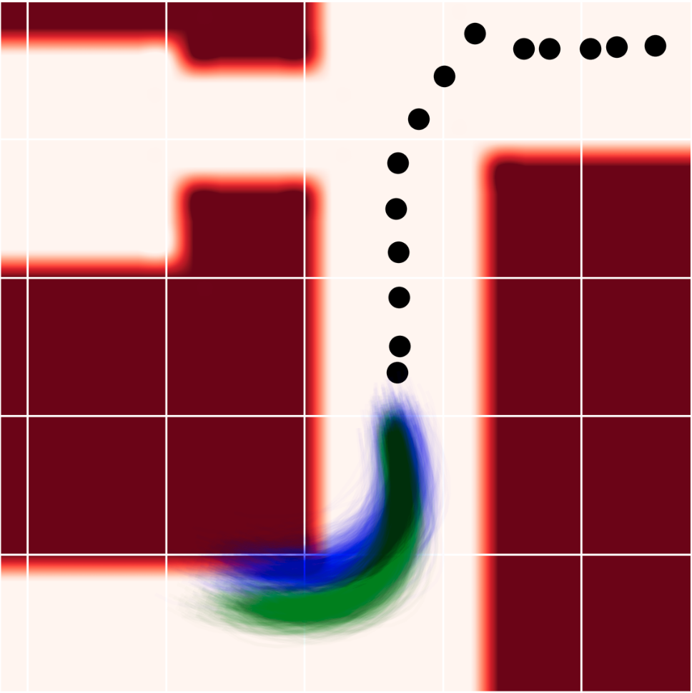
Figure 1: A simple example of enforcing predictions to be consistent with environment: Provided an observed trajectory segment (black), a purely learning method may predict collision-prone distributions of trajectories (blue). Our framework formulates an optimisation problem with chance constraints arising from environmental structure, as given by an occupancy map. We solve to obtain predictions which are compliant with the environment, while remaining similar to the learned future.

II Related Work

Motion Trajectory Prediction. Motion prediction is a problem central to robot autonomy. The most simple methods of motion prediction are physics-based models, such as constant velocity/acceleration models [4]. More complex physics-based models often fuse multiple dynamic models, or select a best fit model from a set [5]. Recent developments in machine learning have led to learning-based methods that learn motion patterns [1, 6] from a dataset of observed trajectories. In particular, long-short term memory (LSTM) and generative adversarial network (GAN)-based models [1, 7, 8, 2] have gained popularity. Methods of learning entire trajectories, similar to our learning component, but with relaxed dependencies, is outlined in [3, 9]. Further attempts to incorporate static obstacles in learning attempt to do so as a part of the learning pipeline [10] and attempts to extrapolate behaviour. Approaches of this kind cannot guarantee that valid solutions satisfy specified chance constraints, and there have not been approaches that directly incorporate occupancy maps, which are typically built by robots from depth sensor data.
Trajectory Optimisation. Trajectory optimisation has been successfully applied in motion planning, by directly expressing obstacles as constraints to solve for collision-free paths between start and goal points. Popular methods include Trajopt [11], CHOMP [12], STOMP [13], and GPMP2 [14]. Trajopt utilises sequential quadratic programming to find locally optimal trajectories compliant with constraints. CHOMP exploits obstacle gradients for efficient optimisation. Further work on gradient-based trajectory optimisation for planning can be found in [15, 16]. Although trajectory optimisation is a popular choice to obtain collision-free trajectories for motion-planning, there has yet to be extensive work in utilising trajectory optimisation for motion prediction. The optimisation required in this work is also different in that we optimise to obtain distributions of trajectories, rather than a single trajectory as required in motion planning.
Combined Learning and Optimisation. There has been previous explorations of combining learning and trajectory optimisation. [17] introduce a framework which combines a known analytical cost function with black box functions in reinforcement learning for manipulation. [18] introduces CLAMP, a framework that combines learning from demonstration with optimisation based motion planning. Theoretical aspects of using learning in conjunction with optimisation, in a Bayesian framework known as posterior regularisation has also been investigated in [19]. All of these methods aim to add more structure to be encoded in learning problems. Similarly our proposed framework allows for encoding of structure, but specifically for the trajectory prediction problem, where we are required to do learning and optimisation on distributions of trajectories with respect to environment occupancy.

III Continuous-time Motion Trajectories

Our framework operates over continuous motion trajectories, capable of being queried at arbitrary resolution, without forward simulating. In this section, we briefly introduce the continuous-time motion trajectory representation used in this work. We restrict ourselves to the 2-D case.

Similar to methods described in [16, 15, 3], we represent motion trajectories as functions $\bm{\xi}:[0,T]\rightarrow\mathbb{R}^{2}$. $T$ represents the prediction time horizon. To we construct our trajectories as dot products between weight vectors and reproducing kernels. We limit our discussion to squared exponential radial basis function (RBF) kernels, though methods in this study generalise to various kernels with minimal modifications. Using RBFs result in smooth trajectories, and have shown good empirical convergence properties for functional trajectory optimisation [15]. A trajectory, $\bm{\xi}(t)$, can be expressed as:

$$\mathbf{\xi}(t)\!=\begin{bmatrix}\mathbf{w}^{x^{\top}}\bm{\phi}(t)\\ \mathbf{w}^{y^{\top}}\bm{\phi}(t)\end{bmatrix}, \mathbf{\phi}(t)\!=\!\left[\phi(t,t^{\prime}_{1}),\dots,\phi(t,t^{\prime}_{M})\right]^{\top},$$ (1)

where the basis functions are given as, $\phi(t,t^{\prime})\!=\!\exp(-\gamma||t-t^{\prime}||^{2})$. The coordinates of a dynamic object at time, $t\in[0,T]$, is given as $x(t)$ and $y(t)$, $\mathbf{w}^{x}$, $\mathbf{w}^{y}\in\mathbb{R}^{M}$ are weight parameters, $\bm{\phi}(t)\in\mathbb{R}^{M}$, and $\bm{t^{\prime}}=[t^{\prime}_{1},t^{\prime}_{2},\ldots,t^{\prime}_{M}]^{\top}$ are $M$ pre-define time points at which RBF kernels are centered. $\gamma$ is a length-scale hyper-parameter which determines the impact a time point neighbouring times on the trajectory.

Motion data typically comes in the form of discrete sequences of timestamped coordinates $\{t_{i},x_{i},y_{i}\},i=0,\dots,N$. To construct a best-fit continuous trajectory of discrete sequences from $N$ timestamped coordinates, we solve the ridge regression problem:

$$\min\limits_{\mathbf{w}^{x},\mathbf{w}^{y}}\sum\limits_{n=1}^{N}\big{\{}(x_{n}-{\mathbf{w}^{x}}^{\top}\bm{\phi}(t_{n}))^{2} +(y_{n}-{\mathbf{w}^{y}}^{\top}\bm{\phi}(t_{n}))^{2}$$

$$+\ldots\lambda(||\mathbf{w}^{x}||^{2}+||\mathbf{w}^{y}||^{2})\big{\}},$$ (2)

where $\lambda$ is a regularisation hyper-parameter, with the set of $M$ uniform times $\bm{t}^{\prime}$ selected a priori, as centers where the kernels are fixed. Evaluating the closed form ridge regression solution results in weight vectors $\mathbf{w}^{x}$ and $\mathbf{w}^{x}$ which forms the trajectory $\bm{\xi}(t)=[{\mathbf{w}^{x}}^{\top}\bm{\phi}(t),{\mathbf{w}^{y}}^{\top}\bm{\phi}(t)]$. We denote the stacked vector of $\mathbf{w}^{x}$ and $\mathbf{w}^{y}$ as $\mathbf{w}$. As future motion trajectories are inherently uncertain, the motion prediction problem often requires predicting a distribution over future trajectories a dynamic object may follow. We denote distributions of trajectories as $\bm{\Xi}$, with the vector of probabilistic weight parameters, $\bm{\omega}$, and the parameters of the distribution over $\bm{\omega}$ is denoted as $\Psi$. $\bm{\Xi}(t)$ gives the distribution of coordinate position at time $t$. Every sample function of $\bm{\Xi}$ is a trajectory $\bm{\xi}$, and samples of vector of random variables $\bm{\omega}$ give $\mathbf{w}$. Denoting the parameter distributions associated with $x$ and $y$ as $\bm{\omega}_{x}$ and $\bm{\omega}_{y}$, distributions of trajectories can be constructed as $\bm{\Xi}=[{\bm{\omega}^{x}}^{\top}\bm{\phi}(t),{\bm{\omega}^{y}}^{\top}\bm{\phi}(t)]$. In practice, to obtain $\bm{\xi}$ we can also sample $\mathbf{w}$ from the distribution $\bm{\omega}$, and take dot products with $\bm{\phi}$.

Figure 2: Overview of our proposed framework. We combine learning and optimisation to generalise data and enforce constraints.

IV Motion Prediction with Environmental Constraints

IV-A Problem Overview

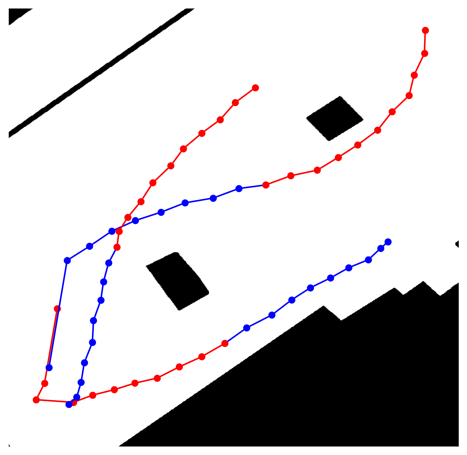
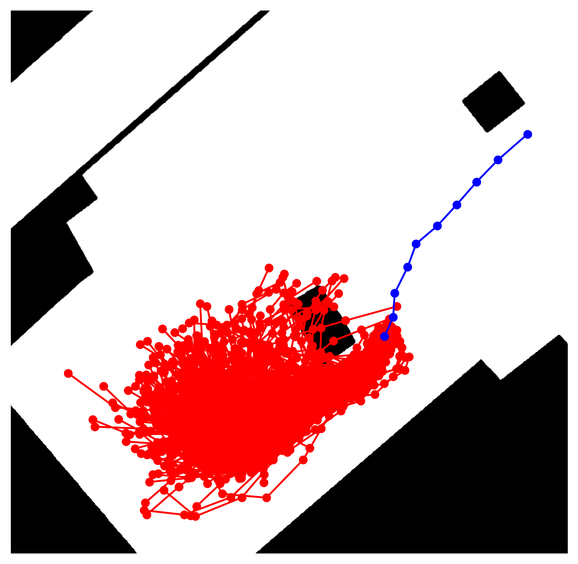
Figure 3: (Left) Examples from real-world dataset [20]. Historical trajectories in blue, and future in red. (Right) Provided a new unseen trajectory (blue), extrapolate futures (red). Learned future trajectories may collide with obstacles. Our framework tackles this by directly enforcing constraints on trajectory distributions, such that the trajectories are collision free.

Our goal is to reason about the possible future trajectories of dynamic objects, based on the immediate past trajectories of the objects, along with occupancy information from the environment. In this work, we limit our discussion to trajectories in 2-D, which usually arise from the tracking of humans and vehicles in video data. We are assumed to have a dataset containing coordinates of an object up to a time, along with its coordinates thereafter, and an occupancy map of the environment. Examples from a real-world dataset are shown in fig. 3, as well as a prediction given by a learning-based model. Given the observed historical coordinates, we aim to extrapolate the distribution of trajectories representing likely future motion thereafter. We require the distribution of trajectories compliant with the environment structure indicated in the occupancy map, such that the probability of hypothesising infeasible trajectories to be constrained to a small value.

IV-B Framework Overview

An overview of our framework is shown in fig. 2. We learn from our training data to predict a vector of random variables of weights $\bm{\omega}_{\Psi_{0}}$ with distribution parameters $\Psi_{0}$, and produce a prior distribution of trajectories, $\bm{\Xi}_{0}$, as described in eq. 1. Our aim is to find an alternative random vector $\bm{\omega}_{\Psi}^{*}$, defined by optimised parameters $\Psi^{*}$, which satisfies enforced constraints, while remaining close to the learned distribution $\bm{\omega}_{\Psi_{0}}$. The optimisation objective uses $\bm{\omega}_{\Psi_{0}}$, while constraints are provided through the obstacle cost operator, $\mathcal{C}$, which requires an occupancy map of the environment. The desired random vector $\bm{\omega}_{\Psi}^{*}$ defines a constraint-compliant distribution of trajectories, $\bm{\Xi}_{\Psi}^{*}$, provided pre-defined RBF features $\bm{\phi}$, by eq. 1. Individual constraint-compliant future trajectories, $\bm{\xi}$, can then be realised from $\bm{\Xi}_{\Psi}^{*}$.

To find the constrain-compliant parameters $\Psi^{*}$, we formulate the optimisation problem in a similar manner to Bayesian posterior regularisation methods [19]. The desired parameters $\Psi^{*}$ is the solution to the constrained optimisation problem:

$$\min_{\Psi}\quad\mathrm{D}_{KL}(\bm{\omega}_{\Psi}\lVert\bm{\omega}_{\Psi_{0}})$$ (3)

$$\textrm{s.t.}\quad\mathcal{C}(\bm{\Xi}_{\Psi})-\epsilon\leq 0$$ (4)

where $\mathrm{D}_{KL}$ is the Kullback-Leibler (KL) divergence [21], and $\mathrm{D}_{KL}(\bm{\omega}_{\Psi}\lVert\bm{\omega}_{\Psi_{0}})$ gives us a definition of “close-ness” between our predicted $\bm{\omega}_{\Psi_{0}}$ and optimised $\bm{\omega}_{\Psi}$ distributions. $\mathcal{C}(\bm{\Xi}_{\Psi})$ is the obstacle cost operator, which maps distributions of trajectories $\bm{\Xi}_{\Psi}$ to a scalar cost value. The cost is interpreted as the time-averaged probability of generating a trajectory that collides with obstacles. We designate $\epsilon$ to be the allowed limit of the obstacle cost. Intuitively, our optimisation problem returns the closest distribution of trajectories, as defined by the KL divergence term, to that given by our predictive model, subject to the obstacle collision constraint. By separating the learning and optimisation, we disentangle the complexities of the learning model and the structural constraints. Our learned $\bm{\omega}_{\Psi_{0}}$ also provides us with a “warm-start” initial solution to our optimisation. In contrast to learning-based approaches, the constraints in our optimisation problem is enforced in valid solutions. The main challenges to solving this trajectory optimisation problem lies in how to obtain the vector of random variables $\bm{\omega}_{\Psi_{0}}$, which defines our prior trajectory distribution $\bm{\Xi}_{0}$, as well as how to derive the obstacle cost operator $\mathcal{C}$ required for optimisation. These are addressed in the following subsections.

IV-C Learning Distributions of Trajectories

In this subsection, we outline a method of learning a mapping from observed historical trajectories to prior distributions of future trajectories, parameterised by $\bm{\omega}_{\Psi_{0}}$. The resulting prior distributions of trajectories are to be used directly in the optimisation problem eq. 4. We model the distribution of trajectories, $\bm{\Xi}$, as mixtures of multi-output stochastic processes. To capture the correlation between x and y coordinates, the distribution over weight parameters are assumed to be mixtures of matrix normal distributions [22]. A matrix normal distribution is the generalisation of the normal distribution to matrix-valued random variables, where each sample from a matrix normal distribution gives a matrix. We work with the matrix of random variables defined by vertically stacking the parameters of coordinate dimensions, denoted as $\mathcal{W}=[\bm{\omega}^{x},\bm{\omega}^{y}]\in\mathbb{R}^{M\times 2}$:

$$\mathcal{W}=\begin{bmatrix}{w}^{x}_{1}&{w}^{y}_{1}\\ \smash{\vdots}&\smash{\vdots}\\ {w}^{x}_{M}&{w}^{y}_{M}\end{bmatrix}, p(\mathcal{W}) =\sum_{r=1}^{R}\alpha_{r}\mathrm{MN}\Big{(}\mathcal{M}_{r},\mathcal{U}_{r},\mathcal{V}_{r}\Big{)}.$$ (5)

We assume that there are $R$ mixture components, similar to a Gaussian mixture model [21], with each component being a matrix normal distribution, and associated weight components $\alpha_{r}$. Matrix normal distributions have location matrices $\mathcal{M}_{r}=[\bm{\mu}_{r}^{x},\bm{\mu}_{r}^{y}]\in\mathbb{R}^{M\times 2}$, and positive-definite scale matrices $\mathcal{U}_{r}\in\mathbb{R}^{M\times M}$, $\mathcal{V}_{r}\in\mathbb{R}^{2\times 2}$ as parameters [23].

We utilise a neural network to learn a mapping from a fixed-length vectorised coordinate sequences, $\bm{\varphi}$, that encodes observed partial trajectories, to component weights $\bm{\alpha}$, along with location matrices $\mathcal{M}_{r}$ the lower triangular $\mathcal{V}_{r}^{\frac{1}{2}}$ and diagonal $\mathcal{U}_{r}^{\frac{1}{2}}$ matrices. $\mathcal{V}$ is positive-definite and will be constructed by taking the product of two lower triangular matrices. The dependence between different times on the trajectory are largely captured the RBF features in the time domain $\bm{\phi}(t)$, as described in section III. Hence, it is sufficient for $\mathcal{U}$ to be a positive definite diagonal matrix. We obtain the input vector $\bm{\varphi}$ by taking a 10 time-step window of the latest observed coordinates, and vectorising to obtain a vector of 20 dimensions. The neural network used is relatively light-weight, consisting of 4 Relu-activated dense layers with number of neurons: $(15\times M\times R)\rightarrow(5\times M\times R)\rightarrow(5\times M\times R)\rightarrow(R\times[3M+3])$. In this work, our main goal is to outline a representation of future trajectories outputted by the network, such that the result can be directly optimised. Our method does not preclude alternative encoding schemes of conditioned history trajectories to be inputted into the network, such as features from LSTM networks [24] or trajectory features outlined in [3].

Provided a dataset of history and future trajectories, given by $N$ pairs of timestamped coordinate sequences. After flattening the history trajectory sequence to obtain $\bm{\varphi}$, and applying eq. 2 on trajectory futures to obtain weight matrices, we have pairs denoted as $\{\bm{\varphi}_{n},\mathcal{W}_{n}\}_{n=1}^{N}$. We learn a mapping from $\bm{\varphi}_{n}$ to parameters $\{\alpha_{r},\mathcal{M}_{r},\mathcal{V}_{r},\mathcal{U}_{r}\}_{r=1}^{R}$ with the fully-connected neural network, with the negative log-likelihood of the weight matrices distributions as the loss function:

$$\mathcal{L} =-\sum_{n=1}^{N}\log$$

$$\dots\sum_{r=1}^{R}\alpha_{r}\frac{\exp\{-\frac{1}{2}\mathrm{tr}[{\mathcal{V}_{r}}^{-1}\!(\mathcal{W}_{n}-\mathcal{M}_{r})^{\top}\!\mathcal{U}_{r}(\mathcal{W}_{n}-\mathcal{M}_{r})]\}}{(2\pi)^{M}|\mathcal{V}_{r}||\mathcal{U}_{r}|^{\frac{M}{2}}}.$$ (6)

and by applying the activation functions:

$$\mathrm{diag}[(\mathcal{U}_{r})^{\frac{1}{2}}] =\exp(z^{\mathrm{diag}(\mathcal{U}_{r})}),$$ (7)

$$\mathrm{LowerTrig}[(\mathcal{V}_{r})^{\frac{1}{2}}] =z^{\mathrm{LowerTrig}(\mathcal{V}_{r})},$$ (8)

$$\mathrm{diag}[(\mathcal{V}_{r})^{\frac{1}{2}}] =\exp(z^{\mathrm{diag}(\mathcal{V}_{r})}),$$ (9)

$$\alpha_{r} =\mathrm{softmax}(z^{\alpha_{r}}),$$ (10)

where $z^{\alpha_{r}},z^{\mathrm{LowerTrig}(\mathcal{V}_{r})},z^{\mathrm{diag}(\mathcal{V}_{r})},z^{\mathrm{diag}(\mathcal{U}_{r})}$ are neural network outputs, and $\mathrm{diag}(\cdot)$, $\mathrm{LowerTrig}(\cdot)$ indicate the matrix diagonal, and strictly lower triangular matrix elements respectively. The $\exp$ activation function guarantees the validity of the scale matrices, by enforcing $z^{\mathrm{diag}(\mathcal{V}_{r})}>0,z^{\mathrm{diag}(\mathcal{U}_{r})}>0$. We also enforce $\sum_{r=1}^{R}\alpha_{r}=1$ using the $\mathrm{softmax}$ function. After we train the neural network, provided a vectorised historical trajectory, $\bm{\varphi}$, the neural network gives the corresponding random vector of weights of our prior trajectory distribution, $\bm{\omega}_{\Psi_{0}}=\mathrm{vec}(\mathcal{W})$, where $\mathrm{vec}(\cdot)$ is the vectorise operator. The prior distributions of trajectories is then the dot product of the trajectory parameters and the RBF features, $\bm{\phi}(t)$, as described in eq. 1.

IV-D Constraints on Distributions of Trajectories

After obtaining the weights, $\bm{\omega}_{\Psi_{0}}$, of a prior distribution of trajectories via learning, our main challenge is to design a cost operator, $\mathcal{C}(\bm{\Xi})$, to encode our desired constraints. Specifically we wish to design $\mathcal{C}(\bm{\Xi})$ to account for collisions of distributions of trajectories, provided an occupancy map. $\mathcal{C}(\bm{\Xi})$ maps a distribution of smooth trajectories, $\bm{\Xi}$, to a real-valued scalar cost, which quantifies how collision-prone a given $\bm{\Xi}$ is. $\mathcal{C}$ differs from the cost operator in trajectory optimisation motion planning problems, such as those in [12, 15, 16], in that the input is a distribution over trajectories rather than a single trajectory. Our optimisation can not only optimise over trajectory mean, but also over trajectory variances.

Like trajectory optimisation methods [12], we assume the cost operator takes the form of average costs over prediction horizon $T$, where the cost at a given point in time, $\mathcal{C}(\bm{\Xi}_{\Psi}(t))$, is the probability of a collision at a given time. $\bm{\Xi}_{\Psi}$ contains weight variables with a distribution parameterised by $\Psi$. We can then interpret $\mathcal{C}(\bm{\Xi}_{\Psi})$ as the average probability of collision over a time horizon, defined as:

$$\mathcal{C}(\bm{\Xi}_{\Psi})= \frac{1}{T}\int\displaylimits_{0}^{T}\mathcal{C}(\bm{\Xi}_{\Psi}(t))\mathrm{d}t$$ (11)

$$= \frac{1}{T}\int\displaylimits_{0}^{T}\int\displaylimits_{\mathbb{R}^{2}}p(m=1|\mathbf{x})p(\mathbf{x}|\Psi,t)\mathrm{d}\mathbf{x}\mathrm{d}t.$$ (12)

The probability of collision at some time and location is computed by taking the product of the probability of the trajectory reaching the coordinate at the given time and the probability that the coordinate is occupied. We are provided with an occupancy map and the probability a coordinate of interest, $\mathbf{x}\in\mathbb{R}^{2}$, being occupied is denoted as $p(m=1|\mathbf{x})$. To evaluate the cost, we could marginalise over the all trajectory parameters, but this may be difficult due to the high dimensionality of $\bm{\omega}$, instead work in the 2-D world space, where the environmental constraints are defined. As $\bm{\Xi}_{\Psi}$ is constructed by taking the dot product of weight vectors and feature vectors, trajectory coordinate distribution in world space at time $t$ is:

$$p(\bm{\Xi}_{\Psi}(t)) \!=\!\sum_{r=1}^{R}\!\alpha_{r}\overbrace{{\mathrm{MN}(\mathcal{M}_{r}^{\top}\bm{\phi}(t),\mathcal{V}_{r},\bm{\phi}(t)^{\top}\mathcal{U}_{r}\bm{\phi}(t)\!)}}^{\text{matrix normal distribution}}$$ (13)

$$\!=\!\sum_{r=1}^{R}\!\alpha_{r}\overbrace{\mathcal{N}(\underbrace{\mathcal{M}_{r}^{\top}\bm{\phi}(t)}_{=:\bm{\mu}_{r}},\underbrace{\bm{\phi}(t)^{\top}\mathcal{U}_{r}\bm{\phi}(t)\mathcal{V}_{r}}_{=:\Sigma_{r}}).}^{\text{multivariate normal}}$$ (14)

By the equivalences between matrix normal and multivariate normal distributions [22], we have a mixture of two-dimensional multivariate normal distributions in world-space, $\bm{\Xi}_{\Psi}(t)\sim\sum_{r=1}^{R}\alpha_{r}\mathcal{N}(\bm{\mu}_{r},\Sigma_{r})$. This is the probability distribution over trajectory coordinates at time $t$, $p(\mathbf{x}|\Psi,t)$. The mixture means and covariances of each component are defined as ${\bm{\mu}_{r}:=\mathcal{M}_{r}^{\top}\bm{\phi}(t)},$ and $\Sigma_{r}:={\bm{\phi}(t)^{\top}\mathcal{U}_{r}\bm{\phi}(t)\mathcal{V}_{r}}.$ Substituting eq. 14 into the inner integral of eq. 12, gives the cost operator equation at given time:

$$\mathcal{C}(\bm{\Xi}_{\Psi}(t))=\sum_{r=1}^{R}\alpha_{r}$$

$$\ldots\int\displaylimits_{\mathbb{R}^{2}}\Big{\{}\frac{\exp[-\frac{1}{2}(\mathbf{x}-\bm{\bm{\mu}_{r}})^{\top}\Sigma_{r}^{-1}\!(\mathbf{x}-\bm{\mu}_{r})]}{(2\pi)|\Sigma_{r}|^{\frac{1}{2}}}\Big{\}}\underbrace{p(m=1|\mathbf{x})}_{\text{From map}}\mathrm{d}\mathbf{x}$$ (15)

Note that $\bm{\mu}_{r}$ and $\Sigma_{r}$ are dependent on $\mathcal{M}_{r},\mathcal{U}_{r},\mathcal{V}_{r}$. During the optimisation, we assume that each mode can be optimised independently and that the importance of each mode, represented by $\alpha$, is accurately captured by the learning model and does not change during trajectory optimisation. We then define the set of parameters to optimise as $\Psi=\big{\{}\mathcal{M}_{r},\mathcal{U}_{r},\mathcal{V}_{r}\}_{r=1}^{R}$. The integral defined in eq. 15 may be intractable to evaluate analytically, so we aim to find an approximation to it. The coordinate distribution at a given time in world space, $\bm{\Xi}_{\Psi}(t)$, is a mixture of bi-variate Gaussian distributions. We use Gauss-Hermite quadrature, suitable for numerically integrating exponential-class functions, to approximate eq. 15. Quadrature methods approximate an integral by taking the weighted sum of integrand values sampled at computed points, called abscissae. We introduce the change of variables, $\bm{z_{r}}=\frac{1}{\sqrt{2}}L_{r}^{-1}(\mathbf{x}-\bm{\mu}_{r})$, where the Cholesky factorisation gives $\Sigma_{r}=L_{r}L_{r}^{T}$. Using Gauss-Hermite quadrature schemes, we have:

$$\mathcal{C}(\bm{\Xi}_{\Psi}(t)) \approx\sum_{r=1}^{R}\alpha_{r}\pi^{-1}\sum_{i=1}^{I}\sum_{j=1}^{J}\beta^{i}\beta^{j}p(m=1|\sqrt{2}L\bm{z}+\bm{\mu}_{r}),$$ (16)

where we find the values of $\bm{z}^{i,j}=[z^{i},z^{j}]^{\top}$ as abscissa obtained from roots of Hermite polynomials, and $\beta^{i}$, $\beta^{j}$ are the associated quadrature weights. Details of abscissae and weight calculations, as well as a review on multi-dimensional Gauss-Hermite quadrature, can be found in [25]. An example of abscissae points when estimating a multi-variate Gaussian is shown in fig. 4. Next, we evaluate the outer integral in eq. 12 using rectangular numerical integration for ${\mathcal{C}(\bm{\Xi}_{\Psi})=\int_{0}^{T}\mathcal{C}(\bm{\Xi}_{\Psi}(t))}\mathrm{d}t$. With $\mathcal{C}(\bm{\Xi}_{\Psi})$ defined, we are in a position to solve the combined learning and constrained optimisation problem, defined earlier in eq. 4, using a non-linear optimisation solver, such as the sequential least squares optimiser SLSQP [26]. Analytical gradients with respect to occupancy is provided when using a continuous differential occupancy map such as those introduced in [27, 28]. By utilising the equivalence between matrix normal distributions and multivariate Gaussians [23], the KL divergence term between $\bm{\omega}_{\Psi}$ and $\bm{\omega}_{\Psi_{0}}$ components can be computed [21]. After obtaining the solution of the optimisation we have the optimised distribution of $\bm{\omega}_{\Psi}^{*}$. By taking dot products between $\bm{\omega}_{\Psi}^{*}$ and $\bm{\phi}$, we can construct $\bm{\Xi}_{\Psi}^{*}$ the constraint-compliant trajectory distribution of futures. Individual realised trajectories $\bm{\xi}$ can then be generated from $\bm{\Xi}_{\Psi}$.

Although we have focused on collision constraints with respect to environment structure, the optimisation allows for constraints on velocity or acceleration. The continuous nature of our trajectories allows time derivatives of trajectories to be obtained. Specifically, the derivative reproducing property, ensures the derivatives of smooth kernels also correspond to kernels [29]. We can reason about the $n^{th}$-order derivatives of displacement by replacing $\bm{\phi}(t)$ with $\frac{\partial^{n}\bm{\phi}(t)}{\partial t^{n}}$.

[capbesideposition=right,top,capbesidewidth=0.3]figure

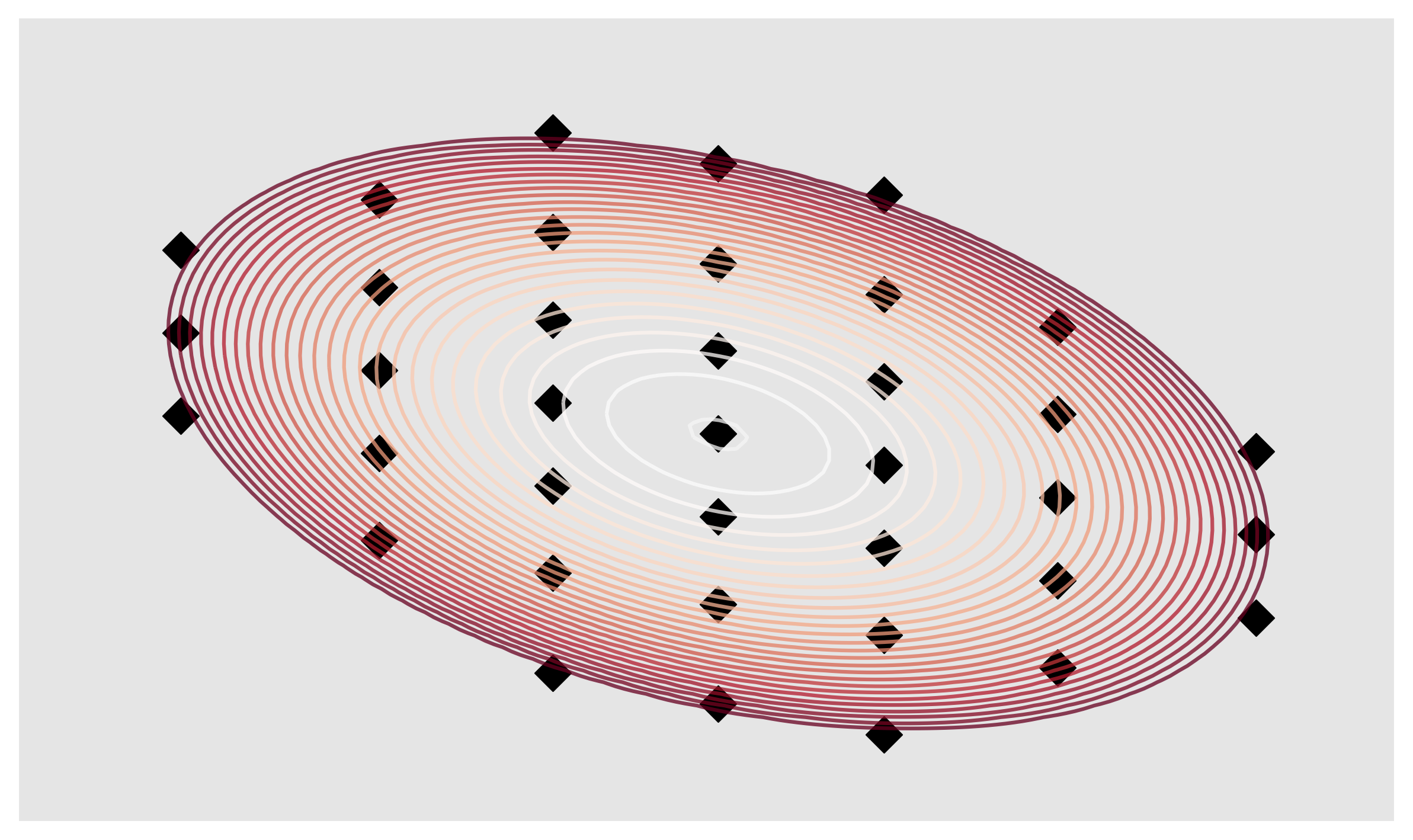
Figure 4: The abscissae (black) for estimating the distribution in world space with the Gauss-Hermite quadrature scheme

V Experimental Evaluation

We empirically evaluate (1) the ability of our learning component to learn probabilistic representations of future trajectories to provide good prior trajectories distributions; (2) the ability of the proposed framework to enforce collision constraints, and its effect on trajectory quality.

V-A Datasets and Metrics

We run our experiments on one simulated dataset, and two real-world datasets, including:

• Simulated dataset (Simulated): This contains simulated trajectories on a floor-plan;

• THÖR dataset [20] (Indoor): This dataset contains real human trajectories walking in a room with three large obstacles in the center of the room.

• Lankershim dataset (Traffic): This dataset contains real vehicle data along a long boulevard. We use a particular busy intersection between $x=[-80,80]$ and $y=[250,500]$.

Throughout each of our experiments, we ensure that the observed trajectory conditioned on contains 10 timesteps. The prediction horizons, $T$, for the simulated, indoor and traffic datasets are 15, 10, and 20 timesteps respectively. We split long trajectories, such that we have 200 pairs of partial trajectories in the simulated dataset, while the indoor dataset contained 871 pairs of partial trajectories, and the traffic dataset contained 6175 pairs. Trajectories that were shorter than the length of the prediction horizon were filtered out. A train-to-test ratio of 80:20 was used for each dataset. For our learning model, we set the number of mixture components $R=2$, hyper-parameters $M=8,10,11$, and $\gamma=0.05,0.1,0.2$ for the simulated, indoors, and traffic datasets respectively. Maps for the simulated and indoor datasets are available, and we construct a map for the traffic dataset by considering the road positions. Our occupancy map is represented as a continuous Hilbert Map [27], giving smooth occupancy probabilities over coordinates, and occupancy gradients.

Metrics used in the quantitative evaluation include: (i) Average displacement error (ADE): The average euclidean distance error between the expectation of the nearest distribution component of trajectories with ground truth trajectory; (iii) Final displacement error (FDE): The euclidean distance error at the end of time horizon between the expectation of the nearest distribution component of trajectories with ground truth trajectory. (iii) Average Likelihood (AL): To take into account the uncertain nature of motion predict, for probabilistic models, we record the likelihood of drawing the trajectory averaged over the timesteps. Note that likelihoods are difficult to interpret and not comparable over different datasets. Lower ADE and FDE, and higher AL indicate better performance. For the evaluation of collisions, we also record the percentage of constraint-violating trajectory distributions in test set.

V-B Learning Continuous-Time Trajectory Distributions as Priors

The trajectory distribution learning component of our framework provides a prior distribution for the optimisation. We examine whether the learning component of our framework is able to learn distributions of future trajectories from data, comparing the performance with several benchmark models. The benchmark models are: (1) Kernel trajectory maps (KTMs) [3], (2) Constant velocity (CV) model, and (3) Naive neural-network (NN) model, where we learn a mapping between past trajectories and future trajectories by minimising the mean squared error loss. The neural network comprised of Relu-activated fully-connect layers with number of neurons: $(560)\rightarrow(180)\rightarrow(180)\rightarrow(N_{t})$, where $N_{t}$ gives the trajectory time horizon.

We see that the learning component of our framework is able to learn high quality distributions of trajectories. Figure 5 shows examples of extrapolated trajectory distributions in red, and the observed trajectory in blue. We see that the learned distribution is relatively close to the ground truth green trajectory, and is able to capture the uncertain nature of motion prediction. Although a non-negligible number of sampled trajectories collide with the environment. Table I summarises the performance results of our method against our benchmarks. We see that our learning model is comparable to the method proposed in [3], while outperforming a constant velocity and naive neural network model. While the KTM method performs slightly better on the traffic dataset, it is purely learning-based and lacks mechanisms to enforce constraints. We note that our method encodes the observed trajectory by simply flattening the input coordinates, as described in section IV-C. More sophisticated methods of encoding the observed trajectory (such as with LSTM networks [24]), independent of our outlined output of trajectory distributions, could improve the performance of the learning model.

		ADE	FDE	AL
Simulated	Ours	1.29	2.27	0.12
	KTM [3]	1.44	2.41	0.11
	CV	4.27	11.66	-
	NN-naive	2.11	6.07	-
Indoors	Ours	0.94	1.32	3.32
	KTM	0.65	1.26	2.88
	CV	2.08	4.66	-
	NN-naive	1.84	3.35	-
Traffic	Ours	4.99	7.24	0.04
	KTM	4.98	7.03	0.043
	CV	5.14	10.38	-
	NN-naive	21.1	39.5	-

TABLE I: We evaluate the quality of our learned trajectory prior with benchmark models. Lower ADE and FDE, and higher AL indicate better performance.

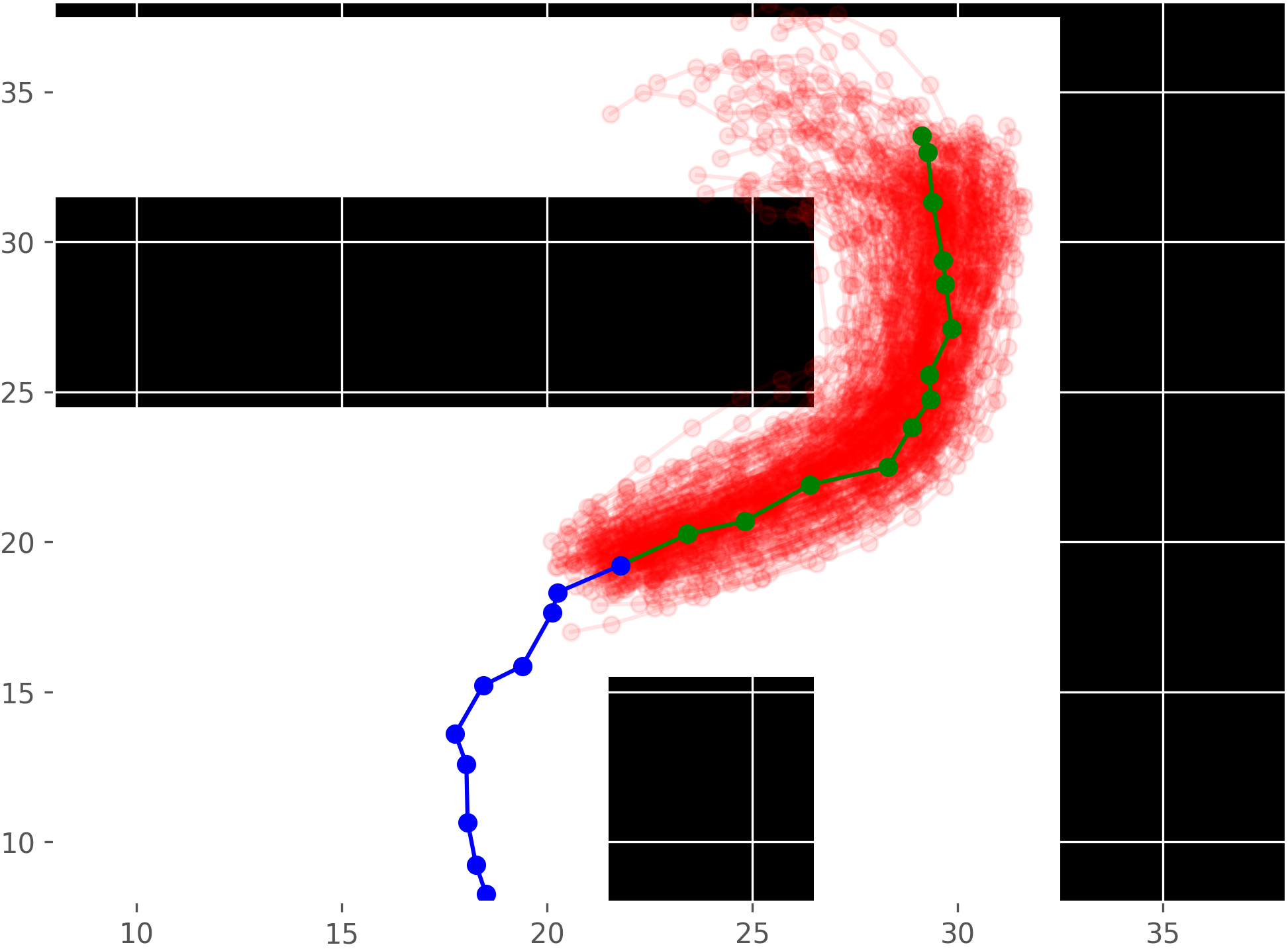
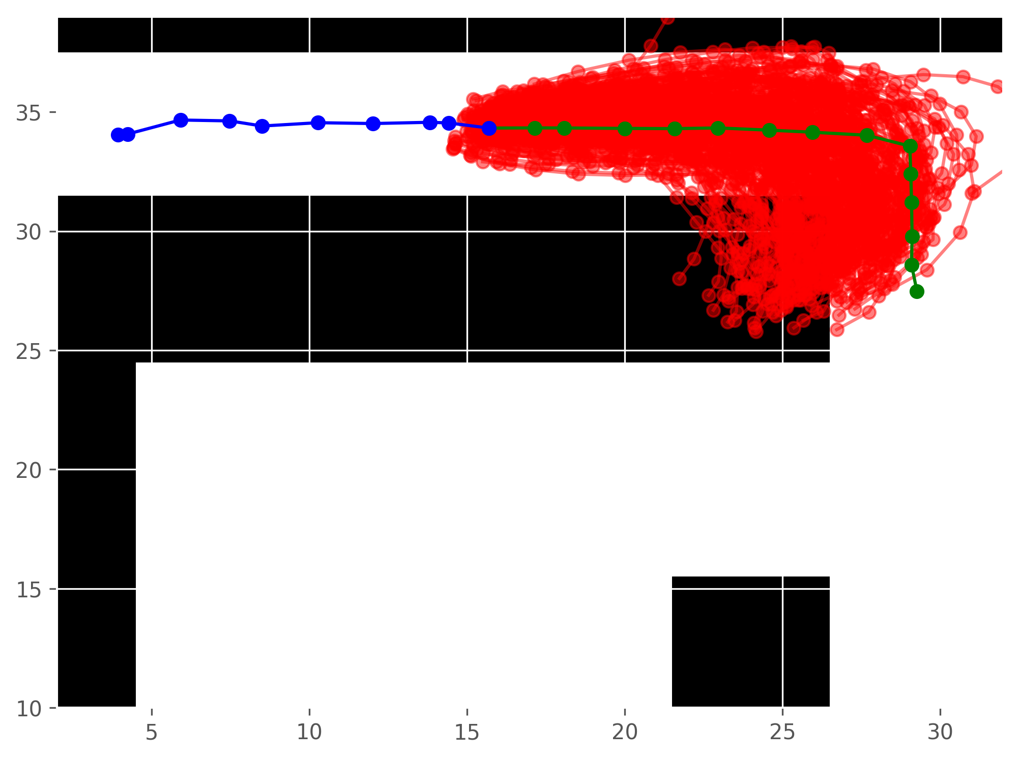
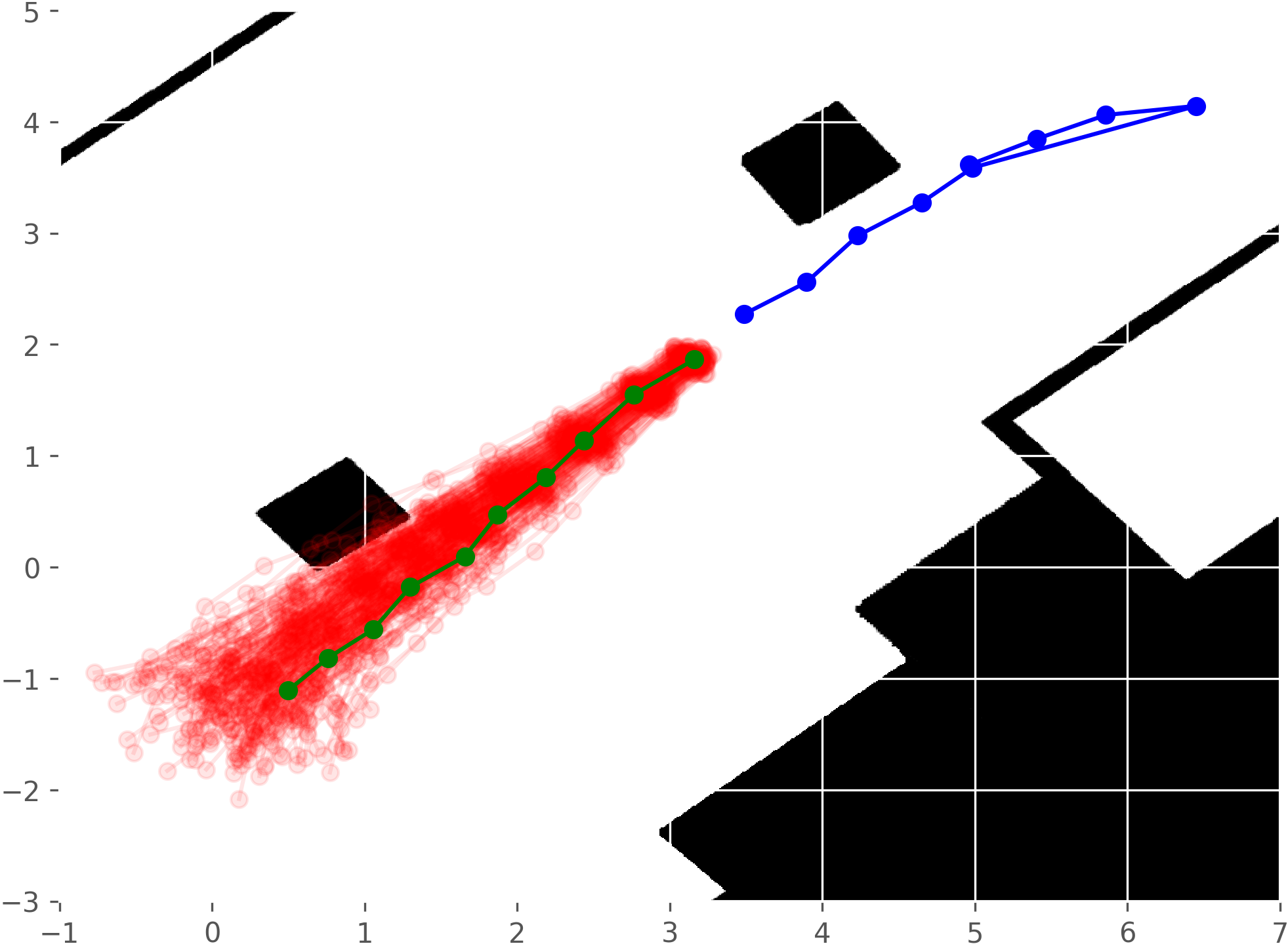
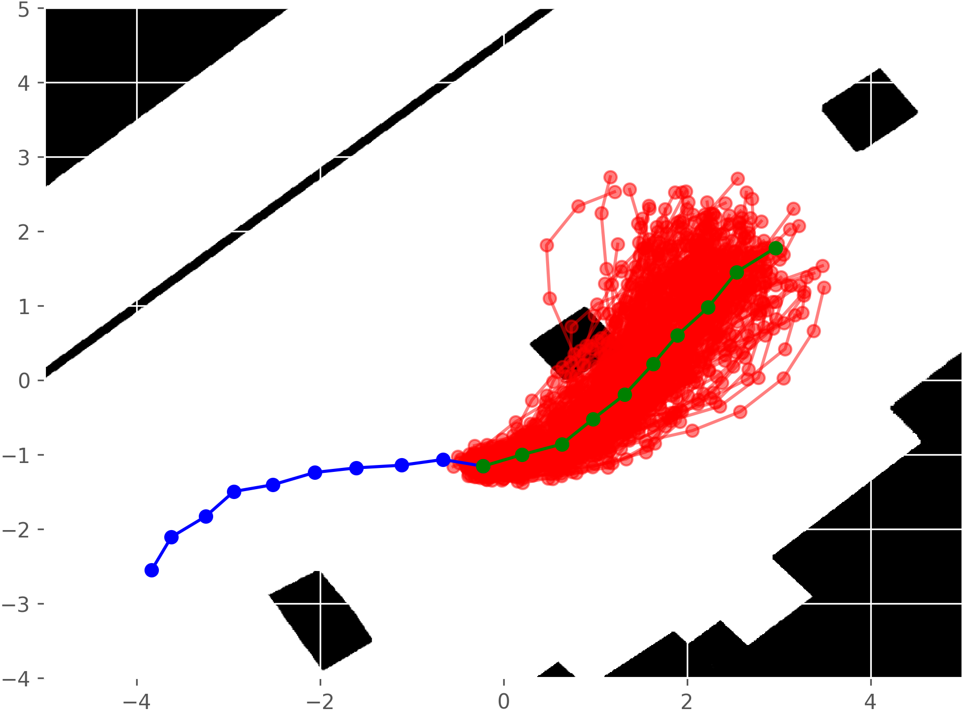
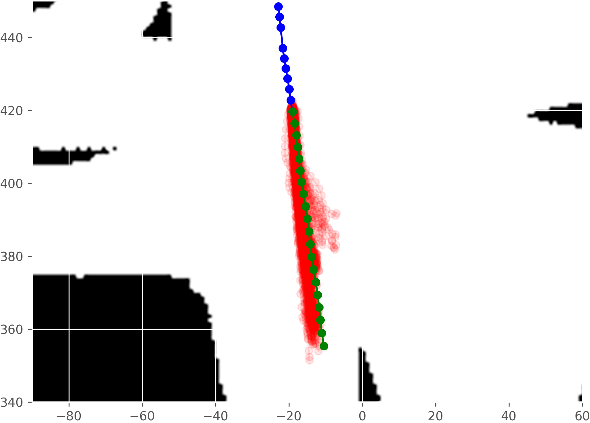
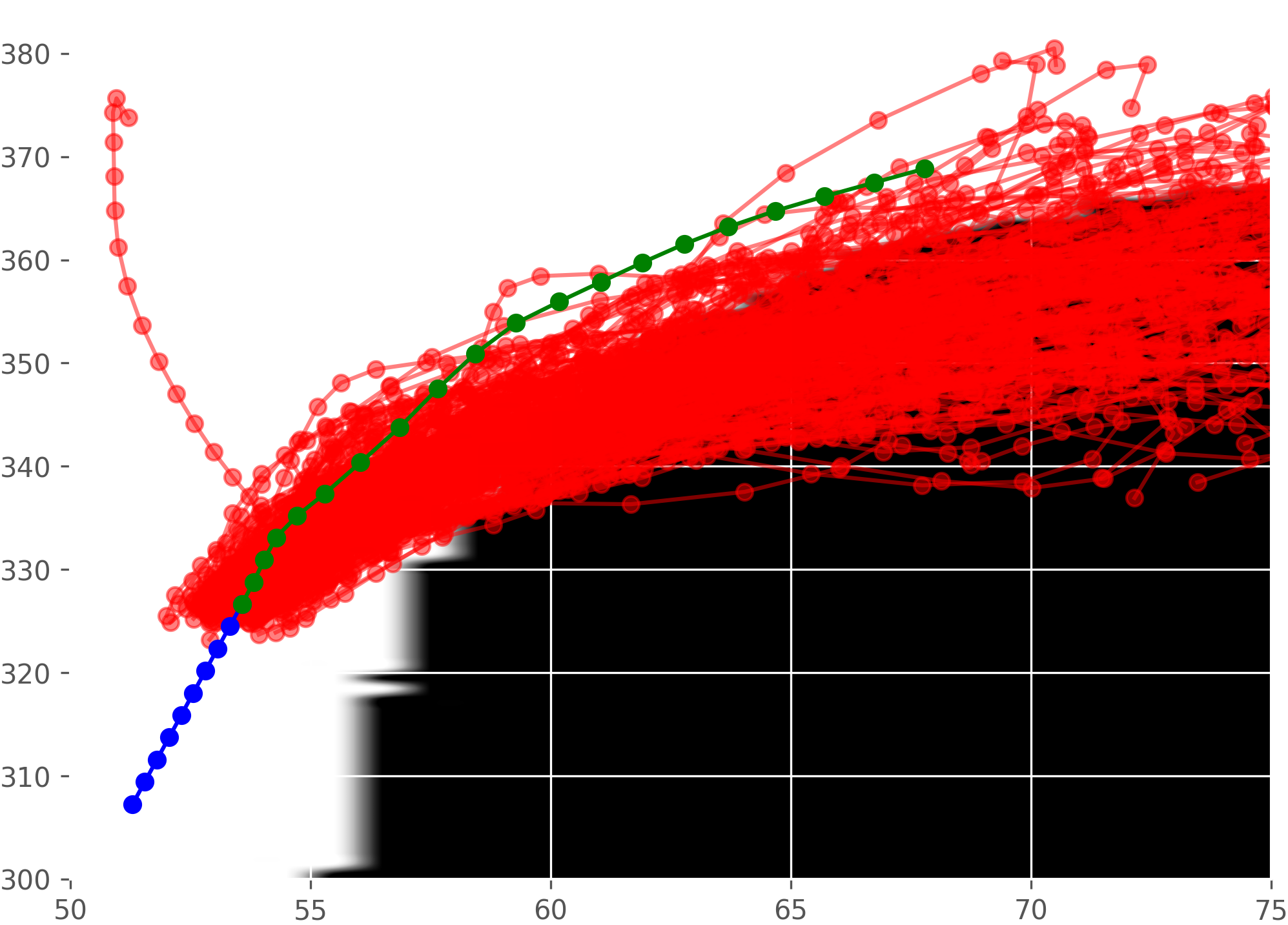
Figure 5: Quantitative evaluations of learned distributions of trajectories (red), Conditioned observations (blue), ground truth (green). We see that our learning model gives relatively good priors, but many sampled trajectories collide with obstacles. The prior distributions are further enforced to be collision-free (See fig. 6)

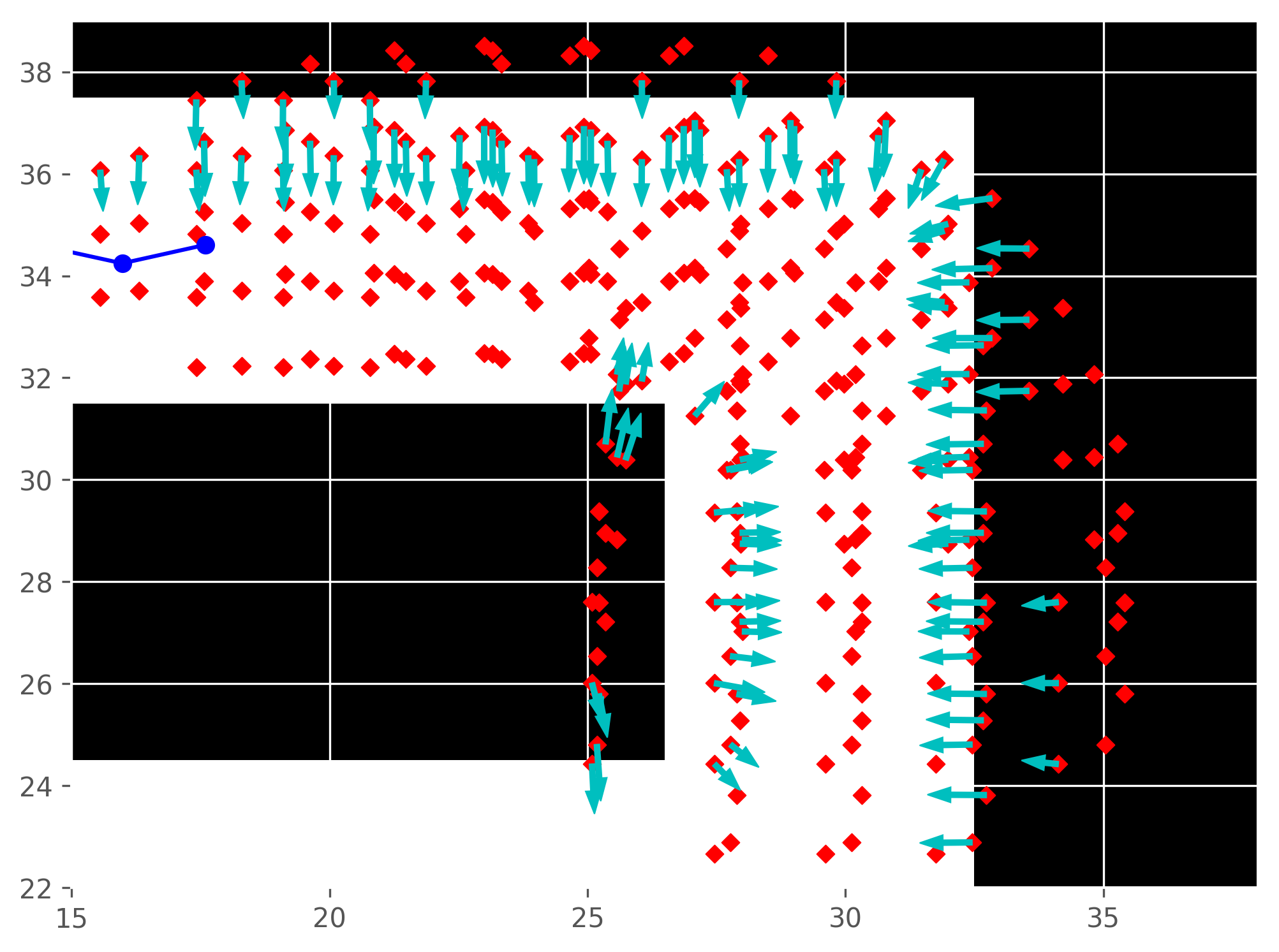
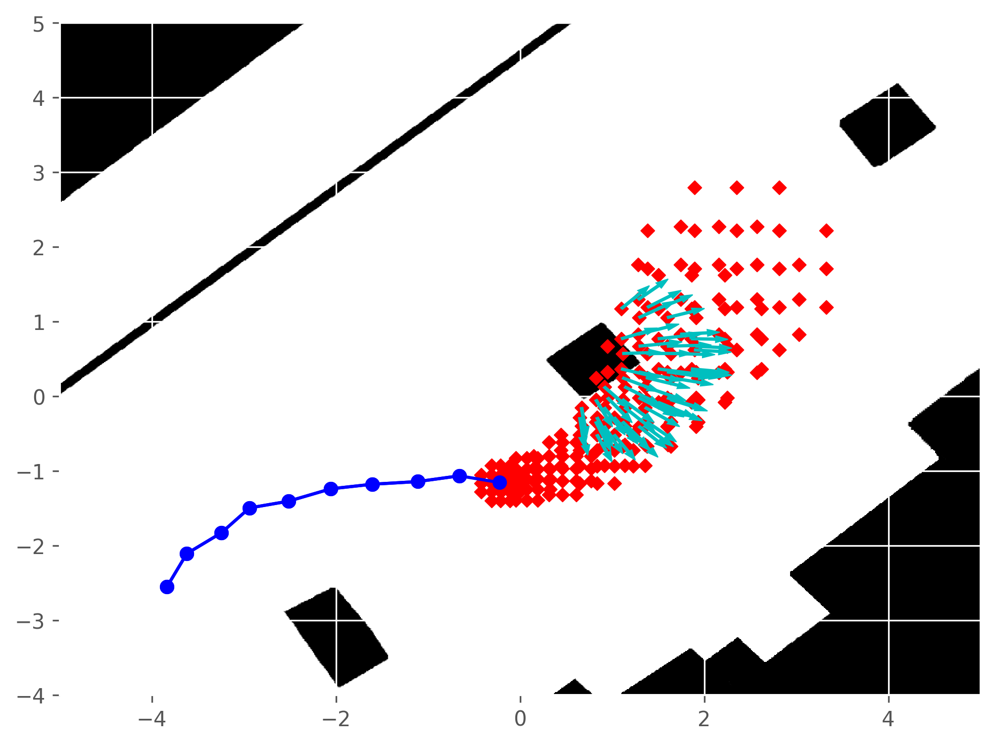
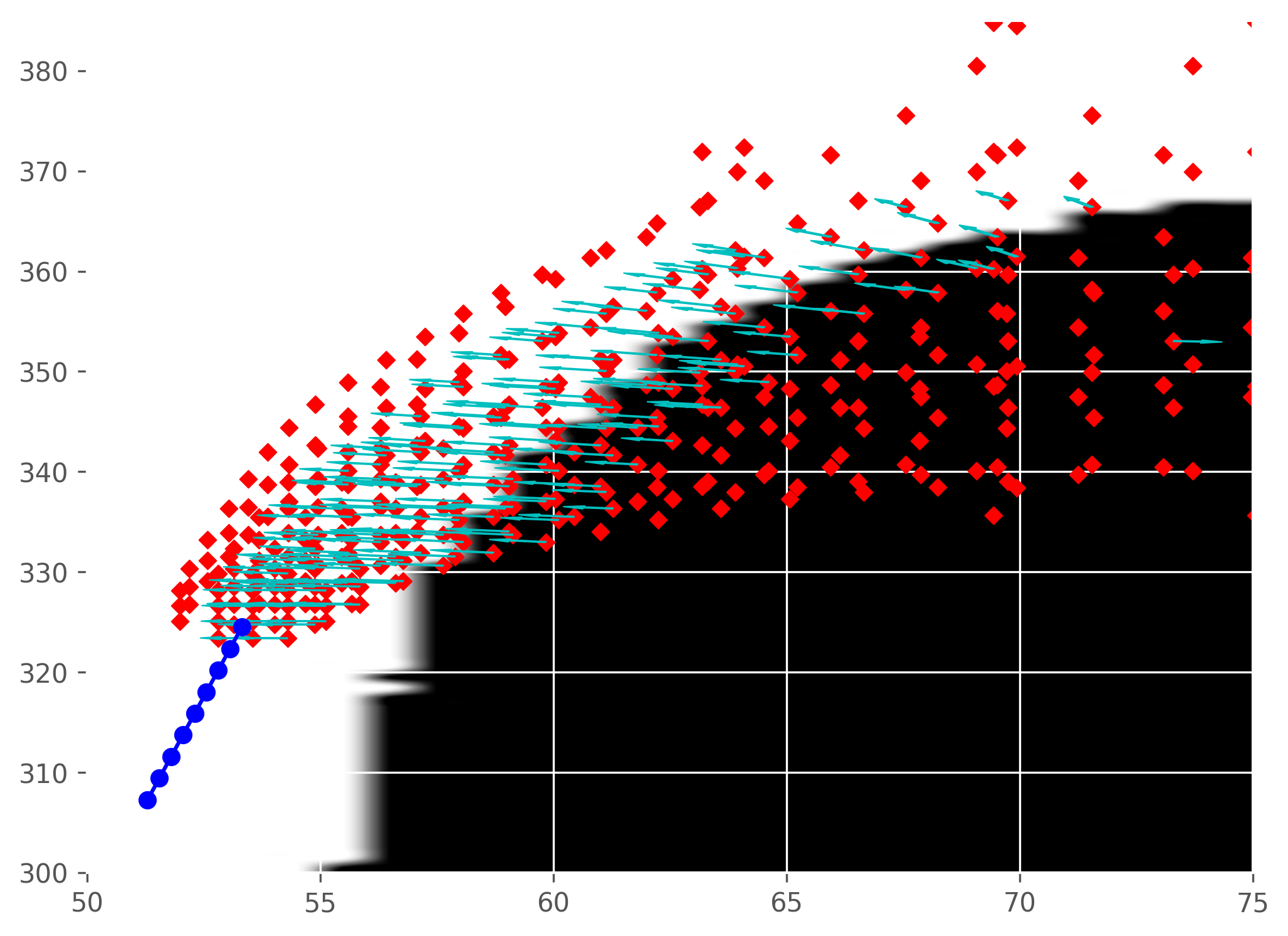
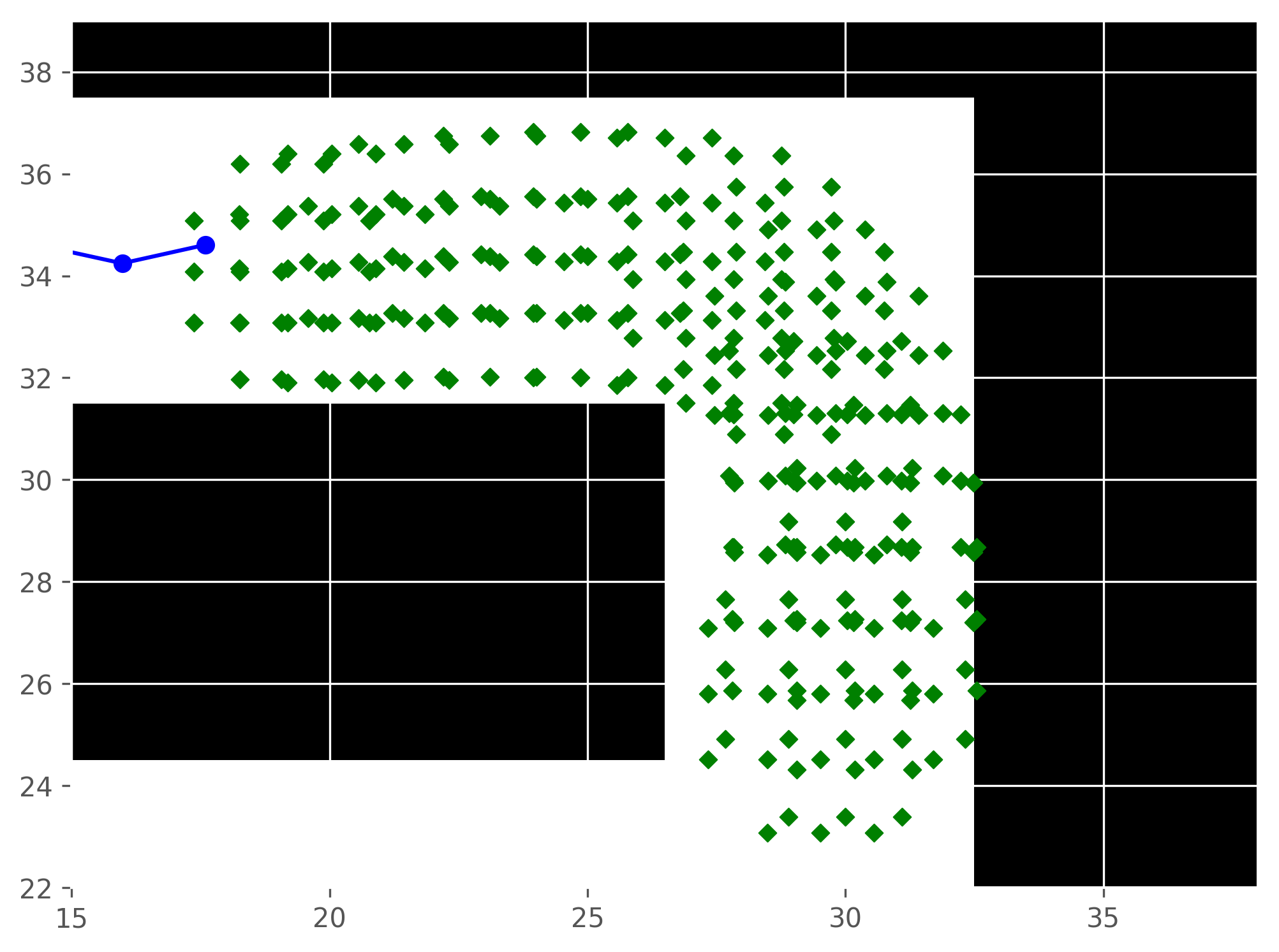
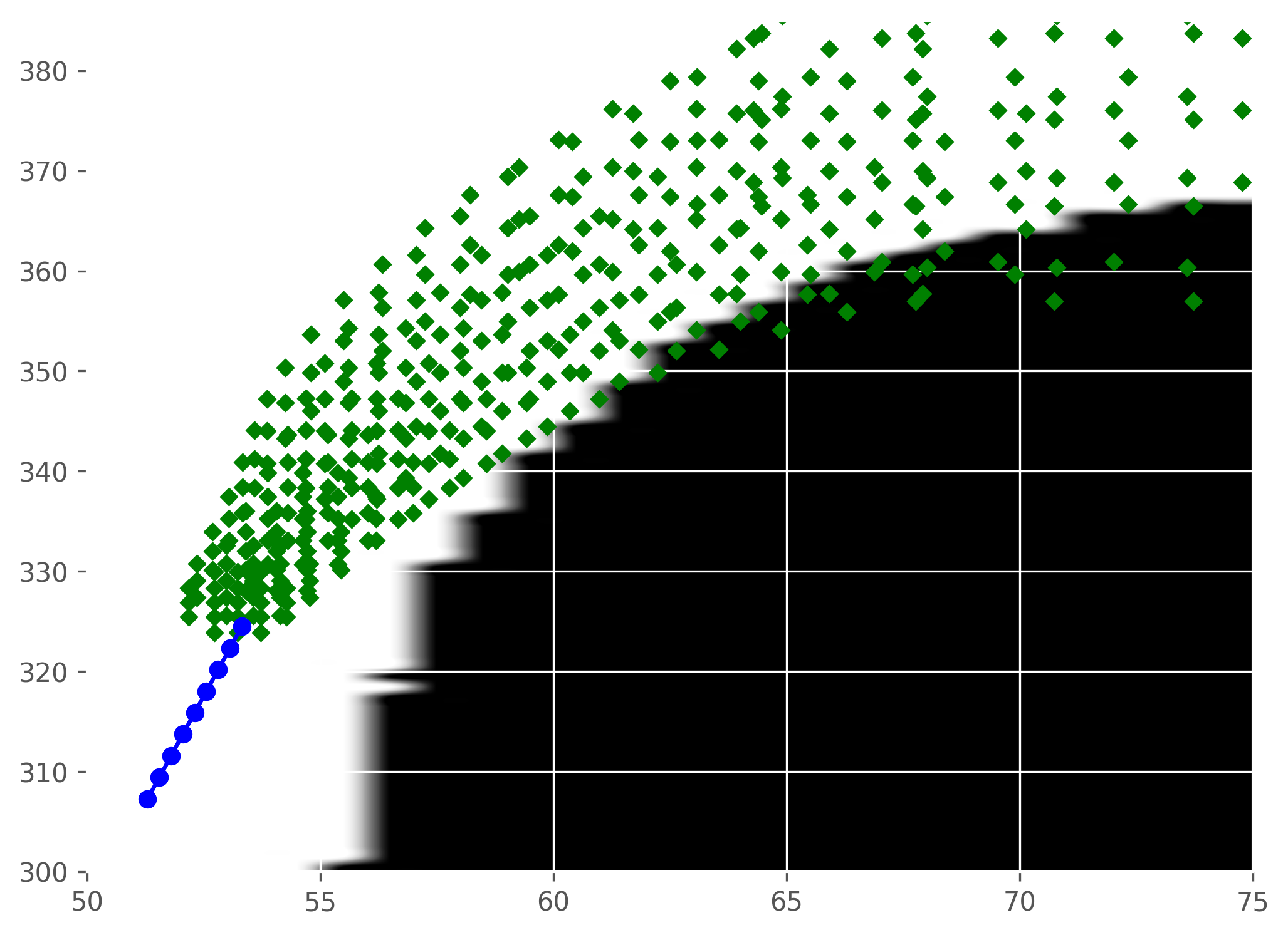
Figure 6: Examples from each dataset of the optimisation component of the framework applying constraints. The top row shows abscissae points of the main component, with notable gradients with respect to occupancy shown as arrows (teal) at the abscissae. The bottom row shows the same abscissae points after optimisation. We see that the constrained distribution subtly conforms better to structures in the environment, while still closely resembling the learned trajectory distribution. The left, middle and right sub-figures are examples from the simulated, indoors, and traffic datasets respectively.

V-C Enforcing Occupancy Compliance via Trajectory Optimisation

After obtaining a prior from our learned model, we apply constraints on the prediction via trajectory optimisation. We will evaluate whether collision constraints can be enforced, and their effect on trajectory quality. We define the constraint such that the time-averaged probability of collision to be less than or equal to 0.05, $\mathcal{C}-0.05\leq 0$. The SLSQP optimiser was able to solve the optimisation quickly, under half a second, with a python implementation. We obtain trajectory distribution priors from our learned model, and select all of the observations where the learned prior trajectory is constraint-violating. We evaluate the performance of the trajectory priors, and compare them with the trajectory distribution predictions after enforcing constraints. The quantitative results are listed in table II. We see after solving with structural constraints, all predictions are feasible. Additionally, the trajectory distribution quality improves after enforcing constraints for all the datasets considered.

		ADE	FDE	AL	C.V.P
Simulated	Unoptimised	1.48	2.87	0.11	40%
	Optimised	1.28	2.33	0.17	0%
Indoors	Unoptimised	1.62	2.41	3.42	15.4%
	Optimised	1.44	2.38	3.3	0%
Traffic	Unoptimised	6.56	11.81	0.034	5.7%
	Optimised	5.14	8.95	0.043	0%

TABLE II: We evaluate the quality of our optimised trajectory distribution with collision constraints, relative to the prior. We see that providing constraints improves prediction quality across all dataset. The percentage of trajectory distributions violating constraint, $\mathcal{C}-0.05\leq 0$, relative to the entire test set is also given, as Constraint Violation Percentage (C.V.P). After optimisation all trajectory distributions are constraint-compliant.

Qualitative results are shown in fig. 6. We see the abscissae points of the largest trajectory distribution component before (top) and after (bottom) the trajectory optimisation of examples in each dataset. Our framework is able to ensure that the distributions comply with environmental structure. Notably, we see that the trajectory optimisation not only adjusts the mean of the trajectory distribution, but also optimises the variances, giving more robust trajectory distributions. This effect is most prominent in the left sub-figure, where the predicted distribution of trajectories in a simulated hallway recovers a much tighter variance which follows the environment structure. We also observe instances collision-avoidance with objects in open space (demonstrated in middle sub-figure), as well as increased adherence to road structure (right sub-figure).

VI Conclusion

We introduced a novel framework to learn motion predictions from observations while conforming to constraints, such as obstacles. Our framework consists of a learning component which learns a distribution over future trajectories. This distribution is used as a prior in a trajectory optimisation step which enforces chance constraints on the trajectory distribution. We empirically demonstrate that our framework can learn complex trajectory distributions and enforce compliance with environment structures via optimisation. This results in reduced variance and the avoidance of obstacles by the predicted trajectories, leading to improved prediction quality.

References

- [1] A. Alahi, K. Goel, V. Ramanathan, A. Robicquet, F.-F. Li, and S. Savarese, “Social lstm: Human trajectory prediction in crowded spaces,” IEEE Conference on Computer Vision and Pattern Recognition, 2016.
- [2] A. Gupta, J. E. Johnson, L. Fei-Fei, S. Savarese, and A. Alahi, “Social gan: Socially acceptable trajectories with generative adversarial networks,” IEEE Conference on Computer Vision and Pattern Recognition, 2018.
- [3] W. Zhi, L. Ott, and F. Ramos, “Kernel trajectory maps for multi-modal probabilistic motion prediction,” Conference on Robot Learning (CoRL), 2019.
- [4] R. Schubert, E. Richter, and G. Wanielik, “Comparison and evaluation of advanced motion models for vehicle tracking,” International Conference on Information Fusion, 2008.
- [5] J. F. P. Kooij, F. Flohr, E. A. I. Pool, and D. Gavrila, “Context-based path prediction for targets with switching dynamics,” International Journal of Computer Vision, 2018.
- [6] W. Zhi, R. Senanayake, L. Ott, and F. Ramos, “Spatiotemporal learning of directional uncertainty in urban environments with kernel recurrent mixture density networks,” IEEE Robotics and Automation Letters, 2019.
- [7] P. Zhang, W. Ouyang, P. Zhang, J. Xue, and N. Zheng, “Sr-lstm: State refinement for lstm towards pedestrian trajectory prediction,” IEEE/CVF Conference on Computer Vision and Pattern Recognition, 2019.
- [8] J. Amirian, J.-B. Hayet, and J. Pettré, “Social ways: Learning multi-modal distributions of pedestrian trajectories with gans,” in CVPR Workshops, 2019.
- [9] W. Zhi, T. Lai, L. Ott, G. Francis, and F. Ramos, “Octnet: Trajectory generation in new environments from past experiences,” 2019.
- [10] A. Sadeghian, V. Kosaraju, A. Sadeghian, N. Hirose, H. Rezatofighi, and S. Savarese, “Sophie: An attentive gan for predicting paths compliant to social and physical constraints,” in Proceedings of the IEEE/CVF Conference on Computer Vision and Pattern Recognition, 2019.
- [11] J. Schulman, J. Ho, A. X. Lee, I. Awwal, H. Bradlow, and P. Abbeel, “Finding locally optimal, collision-free trajectories with sequential convex optimization,” in Robotics: Science and Systems, 2013.
- [12] M. Zucker, N. D. Ratliff, A. D. Dragan, M. Pivtoraiko, M. Klingensmith, C. M. Dellin, J. A. Bagnell, and S. S. Srinivasa, “Chomp: Covariant hamiltonian optimization for motion planning,” The International Journal of Robotics Research, 2013.
- [13] M. Kalakrishnan, S. Chitta, E. Theodorou, P. Pastor, and S. Schaal, “Stomp: Stochastic trajectory optimization for motion planning,” IEEE International Conference on Robotics and Automation, 2011.
- [14] J. Dong, M. Mukadam, F. Dellaert, and B. Boots, “Motion planning as probabilistic inference using gaussian processes and factor graphs,” in Robotics: Science and Systems, 2016.
- [15] Z. Marinho, A. D. Dragan, A. Byravan, B. Boots, S. Srinivasa, and G. J. Gordon, “Functional gradient motion planning in reproducing kernel hilbert spaces,” Robotics: Science and Systems, 2016.
- [16] G. Francis, L. Ott, and F. Ramos, “Fast stochastic functional path planning in occupancy maps,” International Conference on Robotics and Automation (ICRA), 2019.
- [17] P. Englert and M. Toussaint, “Learning manipulation skills from a single demonstration,” International Journal of Robotics Research, 2018.
- [18] M. A. Rana, M. Mukadam, S. R. Ahmadzadeh, S. Chernova, and B. Boots, “Towards robust skill generalization: Unifying learning from demonstration and motion planning,” in Conference on Robot Learning, 2017.
- [19] K. Ganchev, J. a. Graça, J. Gillenwater, and B. Taskar, “Posterior regularization for structured latent variable models,” J. Mach. Learn. Res., 2010.
- [20] A. Rudenko, T. P. Kucner, C. S. Swaminathan, R. T. Chadalavada, K. O. Arras, and A. J. Lilienthal, “Thör: Human-robot navigation data collection and accurate motion trajectories dataset,” IEEE Robotics and Automation Letters, 2020.
- [21] C. M. Bishop, Pattern Recognition and Machine Learning (Information Science and Statistics). 2006.
- [22] A. P. Dawid, “Some matrix-variate distribution theory: Notational considerations and a bayesian application,” Biometrika, 1981.
- [23] P. Dutilleul, “The mle algorithm for the matrix normal distribution,” Journal of Statistical Computation and Simulation, 1999.
- [24] S. Hochreiter and J. Schmidhuber, “Long short-term memory,” Neural Comput., 1997.
- [25] Q. Liu and D. A. Pierce, “A note on gauss-hermite quadrature,” Biometrika, vol. 81, 1994.
- [26] D. Kraft, “A software package for sequential quadratic programming. tech,” tech. rep., DLR German Aerospace Center — Institute for Flight Mechanics, 1988.
- [27] F. Ramos and L. Ott, “Hilbert maps: Scalable continuous occupancy mapping with stochastic gradient descent,” The International Journal of Robotics Research, 2016.
- [28] W. Zhi, L. Ott, R. Senanayake, and F. Ramos, “Continuous occupancy map fusion with fast bayesian hilbert maps,” in 2019 International Conference on Robotics and Automation (ICRA), 2019.
- [29] D.-X. Zhou, “Derivative reproducing properties for kernel methods in learning theory,” Journal of Computational and Applied Mathematics, 2008.