Dynamics of quantum information scrambling under decoherence effects measured via active spins clusters

Abstract

Developing quantum technologies requires the control and understanding of the non-equilibrium dynamics of quantum information in many-body systems. Local information propagates in the system by creating complex correlations known as information scrambling, as this process prevents extracting the information from local measurements. In this work, we develop a model adapted from solid-state NMR methods, to quantify the information scrambling. The scrambling is measured via time-reversal Loschmidt echoes (LE) and Multiple Quantum Coherences experiments that intrinsically contain imperfections. Considering these imperfections, we derive expressions for out-of-time-order correlators (OTOCs) to quantify the observable information scrambling based on measuring the number of active spins where the information was spread. Based on the OTOC expressions, decoherence effects arise naturally by the effects of the nonreverted terms in the LE experiment. Decoherence induces localization of the measurable degree of information scrambling. These effects define a localization cluster size for the observable number of active spins that determines a dynamical equilibrium. We contrast the model’s predictions with quantum simulations performed with solid-state NMR experiments, that measure the information scrambling with time-reversal echoes with controlled imperfections. An excellent quantitative agreement is found with the dynamics of quantum information scrambling and its localization effects determined from the experimental data. The presented model and derived OTOCs set tools for quantifying the quantum information dynamics of large quantum systems (more than $10^{4}$ spins) consistent with experimental implementations that intrinsically contain imperfections.

I introduction

In a quantum many-body system, local information can propagate into many degrees of freedom, creating complex correlations as entanglement that prevents extracting the information from local measurements. This propagation process of information is known as scrambling [1, 2]. Characterizing and understanding the scrambling dynamics is an outstanding problem that connects different fields of physics such as quantum statistical mechanics, cosmology and quantum information processing [3, 4, 5, 6]. The complexity of information scrambling limits our ability to study many-body quantum systems and employ them in technological developments [7, 8]. As many-body systems generate high-order quantum correlations that spread over the system’s degrees of freedom [9, 10, 4, 11, 12, 13], a high degree of scrambling is produced that make these large quantum states more sensitive to perturbations [14, 15, 16, 9, 17, 18].

An accepted measure of scrambling is the tripartite information, which is near maximally negative for quantum channels that scramble the information [19]. This measure proves that information scrambling is manifested through the decay of out-of-time order correlators (OTOCs). OTOCs are special correlators

$$F_{AB}(t) =\frac{1}{|A|\;|B|}\langle A^{\dagger}(t)B^{\dagger}A(t)B\rangle$$ (1)

that quantify the degree of noncommutativity between two local, initially commutating operators $A$ and $B$, where $A(t)=e^{-i\mathcal{H}t}Ae^{i\mathcal{H}t}$ and $\mathcal{H}$ is the Hamiltonian of the interacting system [20, 21, 5]. The decay of the correlator $F_{AB}$ captures the essence of the quantum butterfly effect: a time-evolved local operator fails to commute with almost all the other local operators [22]. The dynamics of $F_{AB}$ is a probe for quantum chaos [23, 24, 25, 26].

The OTOC functions are more accessible experimentally than the tripartite information, therefore these correlators are employed for observing information scrambling in a wide variety of quantum systems using time-reversal of quantum evolutions with Loschmidt echo (LE) experiments [15, 9, 20, 21, 27, 28, 18, 17, 29, 30, 31, 32]. A LE experiment is performed by first evolving forward in time with a Hamiltonian $\mathcal{H}$ and then evolving backward in time with the Hamiltonian $-\mathcal{H}$. A ubiquitous problem of LE experiments is that the forward and backward Hamiltonians are not identical, therefore leading to the existence of nonreverted interactions, such as imperfections or environmental interactions, that introduce nonunitary decays [33, 34, 35, 36, 37, 38]. These decoherence effects add an additional decay to the OTOC functions that should not be confused with the information scrambling generated by the system interactions $\mathcal{H}$. Therefore, it is necessary to model the information scrambling in open quantum systems to correctly interpret scrambling measurements obtained from LE experiments [15, 9, 39, 40, 41, 42, 12, 18, 43].

In this work, we study the dynamics of quantum information scrambling via LE experiments that intrinsically contain imperfections. We show that the scrambling degree can be interpreted as the average number of active spins $K$ [44, 45] –equivalent to a mean Hamming distance– where the information was spread by the evolution that survived the perturbation effects. We derive a more general OTOC than the one described in Eq. (1), that allows modeling decoherence effects induced by the nonreverted terms that affect the outcome of information scrambling measurements. The decoherence effects arise naturally as a leakage of the unitary dynamics of the ideal echo experiment with a rate that depends on the number of active spins. This allows one to model the dynamics of the effective cluster size of correlated spins $K$ that provides a measurable degree of scrambling of information into the system under decoherence effects. We model the OTOCs and the effects of the nonreversed terms in the LE experiments within the framework of the multiple quantum coherences (MQC) technique [15, 9, 20, 27, 28, 29, 18, 17]. The MQC framework was originally developed in solid-state NMR for addressing the dynamics of large interacting quantum systems[46, 47]. Under specific dynamical models, the MQC experiments provide the number of correlated spins $K$ [48, 49, 50], which is an alternative way of interpreting the information scrambling within the spin system [27, 17, 18]. Since solving exactly the dynamics of general and large spin-systems is not possible with present technologies, a variety of models were developed to describe the dynamics of $K$ during the quantum evolution with MQC experiments [51, 46, 47, 52, 53, 54, 55, 56, 57]. We revisit one of these models developed by Levy and Gleason [52] that successfully explained the growth of the cluster size of correlated spins in different crystalline samples [52, 58, 59, 60]. We adapt it to quantify the information scrambling of a local excitation using LE and MQC experiments, including also time-reversal imperfections. The complex dynamics of a multispin system is then simplified, by describing the system quantum state as a mixture of average operators of $L$ active -correlated- spins that have a decoherence decay rate depending on $L$.

We contrast the model’s predictions with quantum simulations performed with solid-state NMR experiments, that measure the information scrambling with time-reversal echoes with controlled imperfections. The presented experiments are based on previous methods and results, where a spin system is quenched by a control Hamiltonian that induces the scrambling of a magnetization that plays the role of a localized initial information [15, 61, 9, 18]. We accurately predict the growth of the cluster size of correlated spins of the experimental data. In particular, our model predicts a localization cluster size of the scrambling dynamics that behaves as a dynamical equilibrium state showing excellent quantitative agreement with the experimental data and previous findings [15, 61]. The model also manifests a transition from a localized to a delocalized dynamics as a function of the perturbation strength in finite systems that might also be related with previous experiments [9]. The quantitative agreement between the model predictions and the experimental data is consistent with a scaling law transition of the decoherence effects of the clusters of active spins where the information is scrambled [18]. Therefore the presented model combined with the derivation of OTOCs can be useful tools to predict the information scrambling dynamics of large quantum systems, and address the effect of imperfections on the control Hamiltonian that drives the quantum evolutions.

Our article is organized as follows. In Sec. II, we introduce the considered spin system, the OTOCs used and how they can be determined with LE and MQC experiments. In Sec. III, we provide a measure for information scrambling based on a cluster size of active –correlated– spins. We also introduce the effects of imperfect echo experiments to quantify the scrambling dynamics. In Sec. IV, we first introduce the original Levy and Gleason model, and then we adapt it to describe quantum information scrambling dynamics. Based on the derived OTOCs, we introduce the decoherence effects induced by imperfection on the time-reversal procedure. In Sec. V, we analyze our model to show how scrambling is modified in the presence of decoherence effects. In Sec. VI, we contrast our model with experimental results, and show the consistency on the predictions of the observable information scrambling bounds measured with NMR quantum simulations. Finally, in Sec. VII we give the conclusions.

II Quantum information scrambling in spin systems

II.1 The system out of equilibrium

We consider a system of $N$ interacting $1/2$ spins in the presence of a strong magnetic field along the $z$ direction. We assume the Larmor frequency $\omega_{z}\gg d_{ij}$, with $d_{ij}$ the dipole-dipole interaction strength between the $i$ and $j$ spins. In a frame of reference rotating at the Larmor frequency, the Hamiltonian of the system is given by the truncated dipolar interaction

$$\mathcal{H} =\mathcal{H}_{dd}$$

$$=\sum_{i<j}d_{ij}\left[2I_{z}^{i}I_{z}^{j}-(I_{x}^{i}I_{x}^{j}+I_{y}^{i}I_{y}^{j})\right],$$ (2)

where we have neglected the nonsecular terms of the dipolar Hamiltonian [62]. Therefore the Hamiltonian $\mathcal{H}_{dd}$ conserves the total magnetization of the system as $[\mathcal{H}_{dd},I_{z}]=0$, with $I_{z}=\sum_{j}I_{z}^{j}$ the total spin operator on the $z$ direction. The operators $I_{v}^{i}$ are the angular momentum of the $i$-th spin in the $v$ direction. We assume the initial-state of the system at a thermal equilibrium with the Zeeman interaction. Its density matrix is $\rho(0)=e^{-\omega_{z}\hbar I_{z}\beta}/\mathrm{Tr}\left(e^{-\omega_{z}\hbar I_{z}\beta}\right)$, where we have neglected the dipolar interaction due to $\omega_{z}\gg d_{ij}$. In the high-temperature limit $\beta^{-1}=k_{B}T\gg\hbar\omega_{z}$, the thermal state is approximated to [62]

$$\rho(0)\sim(\mathbb{I}-\beta\omega_{z}\hbar I_{z})/\mathrm{Tr}\left(\mathbb{I}\right).$$ (3)

The identity operator $\mathbb{I}$ does not evolve over time and does not contribute to the expectation value of an observable magnetization, since $\mathrm{Tr}(I_{v}\mathbb{I})=0$ for any direction $v$. This initial state thus represents an ensemble of local operators $I_{z}^{j}$, that plays the role of an initial local information that will be scrambled into the system degrees of freedom. To induce the spreading of the quantum information from the initial state operator $\rho(0)$, we drive the system away from equilibrium by quenching the Hamiltonian [15, 9, 18]. In NMR, this is typically done by applying rotations to the spins with electromagnetic-field pulses that engineer an average Hamiltonian that does not commute with the initial state [63]. In particular, we consider the effective interaction given by a double-quantum Hamiltonian

$$\mathcal{H}_{0}=\frac{1}{2}\sum_{i,j}d_{ij}(I_{+}^{i}I_{+}^{j}+I_{-}^{i}I_{-}^{j}),$$ (4)

which can be engineered from the dipolar interaction of Eq. (2) via electromagnetic pulse sequences [46]. The Hamiltonian $\mathcal{H}_{0}$ allows one to probe the growth of the number of correlated spins as a function of time [46, 15, 9] as a measure of the degree of scrambling of information into the system [20, 64, 27, 28, 18, 29, 17]. Here, $I_{\pm}^{i}$ are the ladder operators of the $i$-th spin.

In the Zeeman basis, the quantum states $|\vec{m}\rangle=|m_{1},...,m_{N}\rangle$ are characterized by the magnetization numbers $m_{i}=\pm\tfrac{1}{2}$ associated with the local spin operators $I_{z}^{i}$. The double-quantum Hamiltonian flips simultaneously two spins with the same orientation $m_{i}$, therefore inducing transitions from a state $|\vec{m}\rangle$ to a state $|\vec{n}\rangle$ that change the coherence order $M=\sum_{i}m_{i}-n_{i}$ by $\Delta M=\pm 2$. Here $h\left(\vec{m},\vec{n}\right)=M$ is the Hamming distance between the states $|\vec{m}\rangle$ and $|\vec{n}\rangle$. Since the initial state $\rho(0)$ is diagonal, it only has nonvanishing elements for $M=0$ and the double-quantum Hamiltonian only creates even coherence orders.

We consider as our observable the magnetization operator $I_{z}$. The observable signal is then $\mathrm{Tr}\left[I_{z}\rho(t)\right]\propto\mathrm{Tr}\left[I_{z}I_{z}(t)\right]$, which is proportional to the time evolution of the $I_{z}$ operator as the identity term of the initial state gives null trace. Therefore, we consider the evolution of the $I_{z}$ operator. At the evolution time $t$, the scrambled state $I_{z}^{0}(t)=U_{0}(t)I_{z}U_{0}^{\dagger}(t)$ can be expanded in coherence orders as

$$I_{z}^{0}(t) =\sum_{M}\sum_{h\left(\vec{m},\vec{n}\right)=M}\langle\vec{m}|I_{z}^{0}(t)|\vec{n}\rangle\;|\vec{m}\rangle\langle\vec{n}|$$

$$=\sum_{M}I_{z,M}^{0}(t),$$ (5)

where the operator $I_{z,M}^{0}=\sum_{h\left(\vec{m},\vec{n}\right)=M}\langle\vec{m}|I_{z}^{0}(t)|\vec{n}\rangle\;|\vec{m}\rangle\langle\vec{n}|$ contains all the elements of the density operator involving coherences of order $M$. The superindex zero indicates evolution under the double-quantum Hamiltonian $\mathcal{H}_{0}$, i.e., $U_{0}(t)=e^{-i\mathcal{H}_{0}t}$. The amplitude of each coherence order is $f_{M}^{0}=\mathrm{Tr}\left(I_{z}^{2}\right)^{-1}\mathrm{Tr}\left[I_{z,M}^{0}(t)I_{z,M}^{0\dagger}(t)\right]$, that defines the MQC spectrum [46].

II.2 Measuring information scrambling with Multiple Quantum Coherences

The many-body Hamiltonian $\mathcal{H}_{0}$ scrambles the initial local state into the degrees of freedom of the system. The dynamics of the information spreading is contained in the evolved state $I_{z}^{0}(t)=U_{0}(t)I_{z}U_{0}^{\dagger}(t)$. Usually, the degree of information scrambling is quantified between distant local operators $A$ and $B$ in Eq. (1) [19]. In our case, we consider the observation of scrambling based on monitoring the spreading of an ensemble of local operators $I_{z}$ by its own time evolution $I_{z}^{0}(t)$ via the commutator $[I_{z}^{0}(t),I_{z}]$, as it is accessible by time-reversal echoes common in NMR experiments [64, 27, 28, 18, 29]. Based on Eq. (1), the OTO commutator

$$\frac{1}{\mathrm{Tr}\left(I_{z}^{2}\right)}\left\langle\left[I_{z}^{0}(t),I_{z}\right]\left[I_{z}^{0}(t),I_{z}\right]^{\dagger}\right\rangle=\\ =\frac{2}{\mathrm{Tr}\left(I_{z}^{2}\right)}\left\langle I_{z}I_{z}^{0}(t)I_{z}^{0\dagger}(t)I_{z}^{\dagger}\right\rangle-2\mathrm{Re}\left(F_{I_{z},I_{z}}\right)$$ (6)

is related to the OTOC function $F_{I_{z},I_{z}}=\mathrm{Tr}\left(I_{z}^{2}\right)^{-1}\left\langle I_{z}^{0\dagger}(t)I_{z}^{\dagger}I_{z}^{0}(t)I_{z}\right\rangle$, where $\left\langle\mathcal{O}\right\rangle=\mathrm{Tr}\left(\rho_{\beta}\mathcal{O}\right)$ is the expectation value of an operator $\mathcal{O}$ considering the system on the density-matrix state $\rho_{\beta}$. If the system state is in the infinite temperature limit $\rho_{\beta}=\mathbb{I}$, then $\left\langle\mathcal{O}\right\rangle_{\beta=0}=\mathrm{Tr}\left(\mathcal{O}\right)$. Therefore

$$\lim_{\beta\rightarrow 0}\left[\frac{2}{\mathrm{Tr}\left(I_{z}^{2}\right)}\left\langle I_{z}I_{z}^{0}(t)I_{z}^{0\dagger}(t)I_{z}^{\dagger}\right\rangle-2\mathrm{Re}\left(F_{I_{z},I_{z}}\right)\right]=\\ \frac{1}{\mathrm{Tr}\left(I_{z}^{2}\right)}\left\langle\left[I_{z}^{0}(t),I_{z}\right]\left[I_{z}^{0}(t),I_{z}\right]^{\dagger}\right\rangle_{\beta=0}=\\ \frac{1}{\mathrm{Tr}\left(I_{z}^{2}\right)}\mathrm{Tr}\left\{\left[I_{z}^{0}(t),I_{z}\right]\left[I_{z}^{0}(t),I_{z}\right]^{\dagger}\right\}$$ (7)

quantifies the scrambling of local information on $I_{z}$ due to the evolution driven by $\mathcal{H}_{0}$ in the system at infinite temperature [64, 18, 29].

Determining the MQC spectrum allows one to measure the OTOC functions of Eq. (7) [20]. A scheme of an experimental implementation of a concatenation of quantum evolutions used to extract the MQC spectrum is shown in Fig. 1(a) [46].

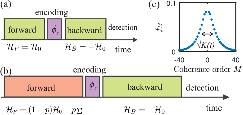
Figure 1: Protocol for measuring multiple quantum coherences and monitoring the quantum information scrambling. (a) The MQC protocol consists of a sequence of quantum evolutions. First, a forward in time evolution is driven by the double quantum Hamiltonian $\mathcal{H}_{F}=\mathcal{H}_{0}$ that pumps coherences of different orders $M$. The rotation $\phi_{z}=e^{iI_{z}\phi}$ encodes the coherence order with a phase $\phi M$. Then a backward in time evolution is driven by the Hamiltonian $\mathcal{H}_{B}=-\mathcal{H}_{0}$ to allow the detection of the MQC spectrum $f_{M}^{0}$ from the signal $f_{0}(t,\phi)=\mathrm{Tr}\left(I_{z}^{2}\right)^{-1}\sum_{M}e^{i\phi M}f_{M}^{0}$. The signal results from measuring the magnetization $I_{z}$, starting from the initial state $\rho(0)=(\mathbb{I}-\beta\omega_{z}\hbar I_{z})/\mathrm{Tr}\left(\mathbb{I}\right)$. (b) Modified MQC protocol to assess the sensitivity of a quantum dynamics to perturbations in the Hamiltonian. The forward Hamiltonian $\mathcal{H}_{F}=(1-p)\mathcal{H}_{0}+p\Sigma$ differs from the backward Hamiltonian $\mathcal{H}_{B}=-\mathcal{H}_{0}$. The resulting MQC spectrum $f_{M}(t,p)=\mathrm{Tr}\left(I_{z}^{2}\right)^{-1}\mathrm{Tr}\left[I_{z,M}^{0}(t)I_{z,M}^{\dagger}(t)\right]$ quantifies the inner product of the coherence orders between the ideal $I_{z}^{0}(t)$ and the perturbed evolution $I_{z}(t)$. (c) Typical form of the MQC spectrum. Its second moment is determined from the squared width of the MQC distribution, and provides a measure for the average number of active spins $K(t)$ where the information was scrambled, shared by the perturbed and unperturbed dynamics.

First, the system is at its initial state, then it is quenched by suddenly turning on the double-quantum Hamiltonian $\mathcal{H}_{0}$. The system evolves forward in time into the scrambled state $I_{z}^{0}(t)=U_{0}(t)I_{z}U_{0}^{\dagger}(t)$. A rotation along the $z$ direction $\phi_{z}=e^{-i\phi I_{z}}$ is applied to the state $I_{z}^{0}(t)$ to label each coherence term $I_{z,M}^{0}(t)$ of Eq. (5), as they acquire a phase $M\phi$. The $I_{z}^{0}(t)$ operator thus becomes

$$I_{z}^{0}\left(\phi,t\right) =\phi_{z}I_{z}^{0}(t)\phi_{z}^{-1}$$

$$=\sum_{M}e^{iM\phi}I_{z,M}^{0}(t).$$ (8)

Finally, the dynamics driven by the double-quantum Hamiltonian $\mathcal{H}_{0}$ is reversed in time by changing the sign of $\mathcal{H}_{0}$ by a pulse sequence design [46]. This backward evolution in time is driven by the evolution operator $U_{0}^{-1}(t)=U_{0}^{\dagger}(t)$. This leads to a many-body Loschmidt echo [33, 34, 37] on the resulting magnetization along $I_{z}$, where we obtain the normalized signal at the end of the evolution:

$$f_{0}(\phi,t) =\frac{1}{\mathrm{Tr}\left(I_{z}^{2}\right)}\mathrm{Tr}\left[I_{z}\ U_{0}^{\dagger}(t)\phi_{z}U_{0}(t)I_{z}U_{0}^{\dagger}(t)\phi_{z}^{\dagger}U_{0}(t)\right]$$

$$=\frac{1}{\mathrm{Tr}\left(I_{z}^{2}\right)}\mathrm{Tr}\left[I_{z}^{0}\left(t\right)I_{z}^{0\dagger}\left(\phi,t\right)\right]$$

$$=\frac{1}{\mathrm{Tr}\left(I_{z}^{2}\right)}\sum_{MM^{\prime}}e^{iM\phi}\mathrm{Tr}\left[I_{z,M}^{0}(t)I_{z,M^{\prime}}^{0\dagger}(t)\right]\delta_{MM^{\prime}}.$$ (9)

We have used the cyclic property of the trace, and the normalization factor $\mathrm{Tr}\left(I_{z}^{2}\right)^{-1}$ to ensure the normalization of the signal $f_{0}(\phi,t=0)=1$. This time-reversal of the quantum dynamics combined with the rotation $\phi_{z}$ allows quantifying the contribution of the different coherence orders $f_{M}^{0}=\mathrm{Tr}\left(I_{z}^{2}\right)^{-1}\mathrm{Tr}\left[I_{z,M}^{0}(t)I_{z,M}^{0\dagger}(t)\right]$ to the global spin state by performing a Fourier transform on $\phi$ [46, 18]. Therefore the scrambling of information into multispin states can be quantified.

As the relevant observable term in the initial state $\rho(0)=(\mathbb{I}-\beta\omega_{z}\hbar I_{z})/\mathrm{Tr}\left(\mathbb{I}\right)$ is proportional to the observable magnetization $I_{z}$, the Loschmidt Echo $f_{0}(\phi,t)$ can be considered as a fidelity between the rotated state $I_{z}^{0}\left(\phi,t\right)$ and the original one $I_{z}^{0}\left(t\right)$ quantified by the inner product $\mathrm{Tr}\left[I_{z}^{0}\left(t\right)I_{z}^{0\dagger}\left(\phi,t\right)\right]$. Moreover, $f_{0}(\phi,t)$ also defines an OTOC function $F_{\phi_{z},I_{z}}$ according to Eq. (7)

$$f_{0}(t,\phi) =\frac{1}{\mathrm{Tr}\left(I_{z}^{2}\right)}\mathrm{Tr}\left[I_{z}^{0}\left(t\right)\phi_{z}I_{z}^{0}\left(t\right)\phi_{z}^{\dagger}\right]$$

$$=F_{\phi_{z},I_{z}}$$

$$=1-\frac{1}{2\mathrm{Tr}\left(I_{z}^{2}\right)}\left\langle\left|\left[I_{z}^{0}(t),\phi_{z}\right]\right|^{2}\right\rangle_{\beta=0},$$ (10)

where again $\mathrm{Tr}(\mathcal{O})=\left\langle\mathcal{O}\right\rangle_{\beta=0}$ is the expectation value of $\mathcal{O}$ with the system state at infinite temperature $\rho_{\beta}=\mathbb{I}$ [64, 18, 29, 65] and we have used that $\left\langle\phi_{z}I_{z}^{0}(t)I_{z}^{0\dagger}(t)\phi_{z}^{\dagger}\right\rangle_{\beta=0}=\mathrm{Tr}\left(I_{z}^{2}\right)$. Using a Taylor expansion as a function of $\phi$ in Eq. (10), the second moment of the MQC spectrum $K_{0}$ is determined by [66, 64, 28, 18]

$$K_{0}=\sum_{M}M^{2}f_{M}^{0}(t)\\ =\frac{1}{\mathrm{Tr}(I_{z}^{2})}\mathrm{Tr}\left(\left[I_{z},I_{z}^{0}(t)\right]\left[I_{z},I_{z}^{0}(t)\right]^{\dagger}\right),$$ (11)

which is related to an OTOC function following Eq. (7). The second moment $K_{0}$ quantifies therefore the information scrambling into the system driven by the double-quantum Hamiltonian $\mathcal{H}_{0}$ starting from the localized information at $I_{z}$.

III Number of active spins as a measure of information scrambling

III.1 Cluster size of correlated spins created by the information scrambling

In the NMR community, the second moment $K_{0}$ is typically used for spin counting of the number of correlated spins by the dynamics induced by a many-body Hamiltonian [46, 48, 50]. The second moment quantifies the cluster size of spins where an initial local state was spread into the system [15, 9]. To relate the second moment of the MQC spectrum $K_{0}$ to a number of correlated spins by the information scrambling, it is necessary to know the propagation model of excitations within the system. Baum et. al. proposed a simple model by assuming that all coherence orders are equally excited for a given system size [46, 47]. The corresponding MQC spectrum has a Gaussian distribution, the second moment of which determines the system size $K_{0}$ which corresponds to the instantaneous number of correlated spins. While this simple assumption works reasonably well in several solid-state systems [67, 48, 52], the MQC distribution is not always Gaussian [49], and other models are required to give a quantitative number of correlated spins [49, 66, 27]. There is no general method to define the number of correlated spins independently of the system dynamics.

We here derive a formal definition for the cluster size of correlated spins from the second moment $K_{0}$ created by the information scrambling, that does not require assumptions regarding the dynamics of the system. This definition for the cluster size is used then in Sec. IV to describe the information scrambling by OTOC functions determined from an imperfect echo experiment.

We consider the product basis $\left\{P_{\vec{u}}=\left(\sqrt{2}\right)^{N}\bigotimes_{i=1}^{N}I_{u_{i}}^{(1)}\right\}$ of the composite Hilbert space for $N$ 1/2-spins, where the index $i$ labels the spins, $u_{i}\in\{0,x,y,z\}$ and $\{I_{u_{i}}^{(1)}\}$ is the set of spin operators of a single $1/2$-spin, including the identity operator $I_{0}^{(1)}\equiv\mathbb{I}$. As these single spin operators satisfy the orthogonal relation $\mathrm{Tr}\left(I_{u_{i}}^{(1)}I_{v_{j}}^{(1)}\right)=\tfrac{1}{2}\delta_{u_{i},v_{j}}$, the operators set $\left\{P_{\vec{u}}\right\}$ is an orthonormal basis of the complete Hilbert space. The evolved quantum state $I_{z}^{0}(t)$ can then be expanded on this basis as

$$I_{z}^{0}(t)=\sum_{\vec{u}}C_{\vec{u}}^{0}(t)P_{\vec{u}},$$ (12)

where $C_{\vec{u}}^{0}(t)$ are time-dependent complex coefficients. Using this expansion, the cluster size of correlated spins is

$$K_{0}(t)=\sum_{\vec{u},\vec{v}}C_{\vec{u}}^{0}(t)C_{\vec{v}}^{0*}(t)\mathcal{L}(\vec{u},\vec{v}),$$ (13)

where ^∗ is the complex conjugate. The function $\mathcal{L}(\vec{u},\vec{v})$ has a functional dependence on $\vec{u}$ and $\vec{v}$ defined by (see Appendix A for a demonstration)

$$\mathcal{L}(\vec{u},\vec{v})=\begin{cases}L(\vec{u})&\vec{u}=\vec{v},\\ 2&h_{z0}(\vec{u},\vec{v})=0,\,h_{xy}(\vec{u},\vec{v})=2\\ &\mathrm{and}\,\vec{v}=\Pi(\vec{u}),\\ -2&h_{z0}(\vec{u},\vec{v})=0,\,h_{xy}(\vec{u},\vec{v})=2\\ &\mathrm{and}\,\vec{v}\neq\Pi(\vec{u}),\\ 0&\mathrm{Other\,cases.}\end{cases}$$ (14)

The diagonal terms when $\vec{u}=\vec{v}$ give the number $L(\vec{u})$ of elements in $\vec{u}$ that are equal to $x$ or $y$. For the nondiagonal terms $\vec{u}\neq\vec{v}$ , the conditions on the right hand side have to be satisfied simultaneously. The function $h_{z0}(\vec{u},\vec{v})$ is the Hamming distance between $\vec{u}$ and $\vec{v}$ only considering the elements that are equal to zero and $z$. In other words, the condition $h_{z0}(\vec{u},\vec{v})=0$ implies that $u_{i}=v{}_{i}$ for every $u_{i}=0,z$. Similarly, $h_{xy}(\vec{u},\vec{v})$ is the Hamming distance between $\vec{u}$ and $\vec{v}$ only considering the elements that are equal to $x$ and $y$. The condition $\vec{v}=\Pi(\vec{u})$ indicates that the vector $\vec{v}$ is a permutation of vector $\vec{u}$.

The cross terms $\vec{u}\neq\vec{v}$ in Eq. (13) have complex numbers with phases that interfere destructively when they are summed, and therefore their contribution goes to zero as the cluster size $K_{0}(t)$ increases [68]. Therefore the cross terms contribution is negligible for large $K_{0}(t)$, obtaining the cluster size of correlated spins

$$K_{0}(t)\sim\sum_{\vec{u}}\left|C_{\vec{u}}^{0}(t)\right|^{2}L(\vec{u}).$$ (15)

Here the magnitude $L(\vec{u})$ quantifies the number of active spins associated to a coherence transfer process $\langle\vec{n}|P_{\vec{u}}|\vec{m}\rangle$ [44, 45]. The transition element $\langle\vec{n}|P_{\vec{u}}|\vec{m}\rangle\neq 0$ if and only if there are $L(\vec{u})$ spins that flip their state during the transition $|\vec{m}\rangle\rightarrow|\vec{n}\rangle$ or, equivalently $L=h(\vec{m},\vec{n})$ with $h$ the Hamming distance. This implies that $K_{0}$ is the average number of active spins in the state $I_{z}^{0}(t)$ weighted by the coefficients $\left|C_{\vec{u}}^{0}(t)\right|^{2}$ that depends on the quantum dynamics, thus providing an interpretation for the information scrambling in spin systems. The cluster size $K_{0}$ provides the average number of spins correlated by quantum superpositions generated by the information scrambling dynamics. The expression of Eq. (15) for $K_{0}$ is similar to the “average correlation length” introduced by Wei et. al. in Ref. [27], but in their work $K_{0}$ is determined by the average number of spins that does not contain identity operators on the system state. A formal connection between OTOC functions and “average correlation length” is also provided in Ref. [27], but only for a particular noninteracting system defined by a spin-chain network topology. In our case, $L(\vec{u})$ quantifies the number of nonidentity operators and non-$I_{z}$ operators in $P_{\vec{u}}$. Based on Eqs. (13) and (15), we provide an average Hamming distance as a way of quantifying a correlation length which is directly connected with the quantum information spreading derived from the OTOC function in Eq. (11). Moreover, our expression to determine $K_{0}$ and the corresponding OTOC is independent of the spin-network topology, and it does not require assumptions on the MQC dynamics.

III.2 Imperfect echo effects on estimating the information scrambling dynamics

Implementations of echo experiments for measuring the information scrambling from the MQC spectrum, always contain imperfections. They thus lead to a time reversion that is not fully performed, altering the OTOC quantification. Different sources of imperfections might occur induced by i) nonidealities of the control operations and ii) the existence of external degrees of freedom considered as an environment [38]. Both imperfection terms in the Hamiltonian cannot be typically reversed. As a paradigmatic model of these imperfections, we consider a perturbation term $p\Sigma$ in the forward Hamiltonian as generally considered within the Loschmidt echo formalism [36, 35, 37] [see Fig. 1(b)]. The perturbation strength $p$ is a dimensionless parameter and $\Sigma$ is a perturbation Hamiltonian. This perturbation spoils the time reversion process and thus induces decoherence effects [15, 9, 18, 38]. As shown in Fig. 1(b), the forward evolution is driven by the evolution operator $U_{P}(t)=e^{-i\mathcal{H}(p)t}$, where the forward Hamiltonian is $\mathcal{H}_{F}=\mathcal{H}(p)=(1-p)\mathcal{H}_{0}+p\Sigma.$ After the forward evolution, again the global rotation $\phi_{z}=e^{-i\phi I_{z}}$ encodes the coherence orders as $\phi_{z}I_{z}(t)\phi_{z}^{\dagger}=\sum_{M}e^{-iM\phi}I_{z,M}(t)$, and then the system is evolved backward in time with an ideal evolution operator $U_{0}^{-1}=e^{it\mathcal{H}_{0}}$. The resulting state is then projected on $I_{z}$, which is the observable magnetization, leading to the signal

$$f(\phi,t,p)=\\ \frac{1}{\mathrm{Tr}\left(I_{z}^{2}\right)}\mathrm{Tr}\left[I_{z}\ U_{0}^{\dagger}(t)\phi_{z}U_{p}(t)I_{z}U_{p}^{\dagger}(t)\phi_{z}^{\dagger}U_{0}(t)\right]\\ =\frac{1}{\mathrm{Tr}\left(I_{z}^{2}\right)}\sum_{M}e^{-iM\phi}\mathrm{Tr}\left[I_{z,M}^{0}(t)I_{z,M}^{\dagger}(t)\right].$$ (16)

The MQC spectrum is now defined by the inner product between the coherence orders of the forward and backward density matrix terms

$$f_{M}(t,p)=\mathrm{Tr}\left(I_{z}^{2}\right)^{-1}\mathrm{Tr}\left[I_{z,M}^{0}(t)I_{z,M}^{\dagger}(t)\right].$$ (17)

As the time reversion evolution is not ideal, therefore it compares the two different information scrambling dynamics by comparing the terms $I_{z,M}^{0}(t)$ and $I_{z,M}(t)$ based on the inner product in $f_{M}$. As derived in Eq. (10), the Loschmidt echo of Eq. (16) can be recast as

$$f(\phi,t) =\frac{1}{\mathrm{Tr}\left(I_{z}^{2}\right)}\mathrm{Tr}\left[I_{z}^{0}(t)I_{z}^{\dagger}(t)\right]-$$

$$-\frac{1}{2\mathrm{Tr}\left(I_{z}^{2}\right)}\mathrm{Tr}\left(\left[\phi_{z},I_{z}^{0}(t)\right]\left[\phi_{z},I_{z}(t)\right]^{\dagger}\right)$$

$$=f(\phi=0,t)-$$

$$-\frac{1}{2\mathrm{Tr}\left(I_{z}^{2}\right)}\mathrm{Tr}\left(\left[\phi_{z},I_{z}^{0}(t)\right]\left[\phi_{z},I_{z}(t)\right]^{\dagger}\right).$$ (18)

Here, the Loschmidt echo is related to a more general OTO commutator $\mathrm{Tr}\left(I_{z}^{2}\right)^{-1}\mathrm{Tr}\left(\left[\phi_{z},I_{z}^{0}(t)\right]\left[\phi_{z},I_{z}(t)\right]^{\dagger}\right)$ than the one described in Eq. (1). This OTOC quantifies the overlap between the commutators $\left[\phi_{z},I_{z}^{0}(t)\right]$ and $\left[\phi_{z},I_{z}(t)\right]$ via the inner product [18]. The second moment of the MQC spectrum $f_{M}(t,p)$ is now

$$\sum_{M}M^{2}f_{M}(t) =\frac{1}{\mathrm{Tr}(I_{z}^{2})}\mathrm{Tr}\left(\left[I_{z},I_{z}^{0}(t)\right]\left[I_{z},I_{z}(t)\right]^{\dagger}\right).$$ (19)

In this imperfect echo experiment, the cluster size is then

$$K(t)=\tfrac{\sum_{M}M^{2}f_{M}(t)}{f(\phi=0,t,p)},$$ (20)

where the second moment of the MQC spectrum must be normalized to the fidelity $f(\phi=0,t,p)=\mathrm{Tr}\left(I_{z}^{2}\right)^{-1}\mathrm{Tr}\left[I_{z}^{0}(t)I_{z}^{\dagger}(t)\right]$. This normalization is required to extract the MQC distribution width, as the fidelity decays as a function of time, and therefore the overall amplitude of the MQC distribution. The second moment $K(t)$ is an effective cluster size that represents the common number of correlated spins between the ideal and the perturbed information scrambling dynamics, quantified by the commutators $\left[I_{z},I_{z}^{0}(t)\right]$ and $\left[I_{z},I_{z}(t)\right]$ respectively [18].

By expanding $I_{z}(t)$ in the basis of the multispin product operators $\left\{P_{\vec{u}}\right\}$,

$$I_{z}(t)=U_{p}(t)I_{z}U_{p}^{\dagger}(t)=\sum_{\vec{u}}C_{\vec{u}}^{p}(t)P_{\vec{u}},$$ (21)

the perturbed version of Eq. (13) is

$$K(t) =\frac{1}{f(\phi=0,t,p)}\sum_{\vec{u},\vec{v}}C_{\vec{u}}^{0}(t)C_{\vec{v}}^{p*}(t)\mathcal{L}(\vec{u},\vec{v}),$$ (22)

where $\mathcal{L}(\vec{u},\vec{v})$ is defined as in Eq. (14). Again, the cross-terms in Eq. (22) are negligible when $K(t)$ is large [68], and we obtain

$$K(t) \simeq\frac{1}{f(\phi=0,t,p)}\sum_{\vec{u}}C_{\vec{u}}^{0}(t)C_{\vec{u}}^{p*}(t)L(\vec{u})$$

$$=\frac{1}{\sum_{\vec{u}}C_{\vec{u}}^{0}(t)C_{\vec{u}}^{p*}(t)}\sum_{\vec{u}}C_{\vec{u}}^{0}(t)C_{\vec{u}}^{p*}(t)L(\vec{u}).$$ (23)

This expression demonstrates that $K(t)$ is an average Hamming distance based on the active spins, weighted by the product between the forward and backward coefficients $C_{\vec{u}}^{0}(t)C_{\vec{u}}^{p*}$ that determine the respective dynamics evolutions. Therefore the expression we derived here for $K(t)$ gives the average number of active spins shared by the forward and backward dynamics. As experimental implementations of time reversions have always a nonreverted interaction, our expression for $K(t)$ provides a definition of what is actually measured as information scrambling with echo experiments.

IV Model for the dynamics of quantum information scrambling under decoherence

IV.1 Revisiting the Levy-Gleason model: Quantum information scrambling dynamics

We develop a phenomenological model to describe the time evolution of the information scrambling observed via the second moment of the MQC distribution $K(t)$. Levy and Gleason developed a model to describe the MQC dynamics in solid state systems [52]. We here adapt this model for determining the information scrambling dynamics in a spin system by using the expressions of Eqs. (15) and (23).

As the complexity of many-spin system dynamics is an outstanding problem in physics that only allows one to obtain exact solutions for $I_{z}(t)$ for very special cases [69, 70, 71, 72, 73], approximations or phenomenological models need to be implemented [51, 46, 52, 47, 74, 53, 75, 68, 54]. The Levy-Gleason model describes the growth of the cluster size of correlated spins $K_{0}(t)$ as a function of time by introducing average operators that contains all the elements of the product operator basis with the same number of nonidentity operators. Instead, based on the result of Eq. (15), which shows that the active spins are the relevant ones for quantifying the information scrambling dynamics, we adapt the Levy-Gleason model by defining an average operator $P_{L}$ of the operators $P_{\vec{u}}$ that contain $L$ active spins, defined by the number of nonidentity and non-$I_{z}$ operators, as described in Sec. III.1. The time evolution of the $I_{z}$ operator is thus

$$I_{z}^{0}(t)=\sum_{\vec{u}}C_{\vec{u}}^{0}(t)P_{\vec{u}}\approx\sum_{L}C_{L}^{0}(t)P_{L}.$$ (24)

Applying the Liouville-von Neumann equation to Eq. (24), the dynamics of the coefficients $C_{L}^{0}(t)$ is determined by the set of $N$ coupled linear differential equations

$$\frac{d}{dt}C_{L}^{0}=-\frac{i}{4}W_{L-1}C_{L-1}^{0}-\frac{i}{4}W_{L}C_{L+1}^{0},$$ (25)

where $W_{L}$ and $W_{L-1}$ are the transition probabilities of increasing or reducing the number of active spins $L(\vec{u})$ by one spin respectively. Following the Levy and Gleason assumptions, we consider that the operator $P_{L}$ represents a contiguous group of $L$ spins in real space, and that the only relevant interactions are between near neighbors. Therefore, the transition probability $W_{L}$ is determined by an effective dipolar coupling strength $d$ multiplied by the number of spins at the cluster edge $L^{\delta}$, where the exponent $\delta$ can be estimated from the the spatial dimension $D$ of the system as $\delta\sim 1-1/D$. The effective coupling $d$ is of the same order of magnitude as the width of the spins’ resonance line and can be determined from a fit to the experimental data [52]. Based on these assumptions, the transition probability is

$$W_{L}=dL^{\delta},$$ (26)

as a function of the number of active spins $L$.

Our results of Sec. III.1 that derive Eq. (15), show that the second moment $K_{0}(t)$ and hence the information scrambling of Eq. (11), are determined by the average number of active spins weighted by the dynamics coefficients $|C_{L}(t)|^{2}$

$$K_{0}(t)=\sum_{L}L|C_{L}^{0}(t)|^{2}.$$ (27)

Its time evolution can then be obtained by solving a set of $N$ differential equations rather than $2^{N}$ as in the exact Liouville-von Neumann equation for an $N$ spin system. Therefore, the connection between the cluster size of correlated spins and the second moment of the MQC spectrum arises naturally based on the average number of active spins involved in the information scrambling correlations. The consistency of this assumption relies on the fact that the Levy and Gleason model reproduced well several experimental results in solid-state systems where power-law growth of the cluster size evolution is seen [52]. The predicted growth rates and power-law exponents were also consistent with the spin-spin coupling network topologies.

IV.2 Model for the decoherent dynamics of quantum information scrambling

We now consider that decoherence effects or perturbations to the ideal Hamiltonian affect the time reversion of the protocol described in Sec. II.2. The product of the two complex coefficients $C_{\vec{u}}^{p}$ and $C_{\vec{u}}^{0}$ of the forward and backward dynamics, respectively, in Eq. (23), produces a reduction of the effective cluster size $K(t)$ compared to the one determined by the ideal echo experiment case $K_{0}(t)$. For weak perturbations, we consider that the coefficients $C_{\vec{u}}^{0}$ and $C_{\vec{u}}^{p}$ mainly differ by a phase, where $C_{\vec{u}}^{p}\sim|C_{\vec{u}}^{0}|\,e^{i\phi_{\vec{u}}}$. Therefore the cluster size of Eq. (23) is

$$K(t)\sim\frac{1}{f(\phi=0,t,p)}\sum_{\vec{u}}\left|C_{\vec{u}}^{0}(t)\right|^{2}\cos(\phi_{\vec{u}})L(\vec{u}).$$ (28)

We here only consider the real part $\cos(\phi_{\vec{u}})$ of the phase term, since $K(t)$ is real and the imaginary terms cancel out. We then recast Eq. (28) in terms of the number of active spins $L$

$$K(t)\sim\frac{1}{f(\phi=0,t,p)}\sum_{L}L\sum_{\vec{u}_{L}}\left|C_{\vec{u}_{L}}^{0}(t)\right|^{2}\cos(\phi_{\vec{u}_{L}}).$$ (29)

The coefficients $C_{L}^{0}(t)\equiv\sum_{\vec{u_{L}}}\left|C_{\vec{u}_{L}}^{0}(t)\right|^{2}$ of the average operator $P_{L}$, in Eq. (24), need now to be modified as the phase $\cos(\phi_{\vec{u}_{L}})$ introduces an attenuation factor that depends on $L$. The effective cluster size $K$ is now described by the attenuated coefficients $C_{L}(t)=\sum_{\vec{u}_{L}}\left|C_{\vec{u}_{L}}^{0}(t)\right|^{2}\cos(\phi_{\vec{u}_{L}})$, with $\left|C_{L}(t)\right|<\left|C_{L}^{0}(t)\right|$. The perturbation term in the echo experiment is therefore modeled as a source of decoherence in an open quantum system. We model this attenuation by adding to Eq. (25) a leakage term with a rate $\Gamma_{L}$ that destroys the quantum superpositions given by the operator product $P_{L}$,

$$\frac{d}{dt}C_{L}=-\frac{i}{4}W_{L-1}C_{L-1}-\frac{i}{4}W_{L}C_{L+1}-\Gamma_{L}C_{L}.$$ (30)

The rate $\Gamma_{L}$ is the average decoherence rate for the product of $L$ active spin operators. A schematic representation of the model is shown in Fig. 2.

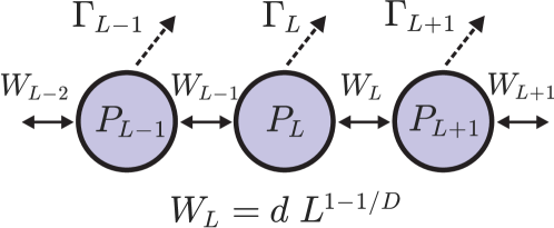
Figure 2: Schematic representation of the model for the decoherent dynamics of quantum information scrambling. It models the evolution of the effective cluster size of active spins $K(t)$ in the presence of decoherence effects induced by a perturbation on the echo experiment described in Fig. 1. The rate $W_{L}$ is the transition probability between $P_{L-1}$ and $P_{L}$, and it is determined by the strength of the dipolar interaction $d$, the size of the cluster of active spins $L$ and the lattice dimension $D$. The spin clusters are affected by a decoherence process, characterized by the decoherence rate $\Gamma_{L}$.

The matrix representation of Eq. (30) is

$$\frac{d}{dt}\vec{C}=-\Upsilon\vec{C},$$

$$\begin{bmatrix}\frac{d}{dt}C_{1}\\ \frac{d}{dt}C_{2}\\ \vdots\\ \frac{d}{dt}C_{N}\end{bmatrix}=-i\begin{bmatrix}-i\Gamma_{1}&\frac{1}{4}W_{1}&0&\cdots&0\\ \frac{1}{4}W_{1}&-i\Gamma_{2}&\frac{1}{4}W_{2}&\cdots&0\\ \vdots&\vdots&\vdots&\ddots&\vdots\\ 0&0&\cdots&\frac{1}{4}W_{N-1}&-i\Gamma_{N}\end{bmatrix}\begin{bmatrix}C_{1}\\ C_{2}\\ \vdots\\ C_{N}\end{bmatrix},$$ (31)

and the effective cluster size $K$ in terms of $C_{L}$, is

$$K(t)=\left[\sum_{L}|C_{L}(t)|^{2}\right]^{-1}\sum_{L}L|C_{L}(t)|^{2}.$$ (32)

If the rate $\Gamma_{L}$ has no dependence on $L$, then all the coefficients $C_{L}$ are affected by a global attenuation factor. The effective cluster size $K(t)$ evolves then equally to the case without perturbation, consistently with the predictions derived in Ref. [64]. However, typically the decoherence effects induced by perturbations increase with the number of active spins that are correlated, and therefore $\Gamma_{L}$ generally depends on $L$ [76, 77, 78, 14, 61, 79, 18].

V Effective cluster size evolution: decoherent dynamics of quantum information scrambling

To analyze the effective cluster size evolution predicted by our model, we consider the diagonal base for $\Upsilon$ to solve Eq. (31)

$$\frac{d}{dt}\tilde{C}_{i}=-\lambda_{i}\tilde{C}_{i},$$ (33)

where $\tilde{C}_{i}$ is the $i$-th component of the populations vector $\vec{C}$ in the eigenbasis of $\Upsilon$, and $\lambda_{i}$ is the the $i$-th eigenvalue. The solution is then

$$\tilde{C}_{i}(t)=\tilde{C}_{i}(0)e^{-\lambda_{i}t},$$ (34)

where $\tilde{C}_{i}(0)$ gives the initial condition $C(0)$ expressed in the $\Upsilon$-eigenbasis. We consider that the decoherence rate increases as a power law with the cluster size of active spins $\Gamma_{L}=\Gamma_{1}L^{\alpha}$, where $\alpha$ is the scaling exponent, as reported in quantum simulations in solid-state spin systems [14, 18] and this dependence is also expected for spin-boson models [76, 77, 78]. We focus on three-dimensional (3D) systems, and thus we set the parameter $\delta=0.66$ in Eq. (26).

We determine the evolution of the cluster size of correlated spins for the case without perturbation. Figure 3(a) shows the cluster size evolution $K_{0}(t)$ for $\Gamma_{1}=0$ and different system sizes $N$. The cluster size grows with a power law as $K_{0}(t)=K_{1}t^{a}$, until it reaches a maximum value due to finite-size effects determined by the system size $N$. The power-law exponent $a$ and the constant $K_{1}$ are determined by the dimension of the system $D$ and the average dipolar coupling $d$ respectively, from Eq. (26). After $K_{0}(t)$ reaches its maximum value, it begins to oscillate indefinitely, again due to finite-size effects. Therefore, this solution is only useful before finite-size effects dominate the dynamical behavior.

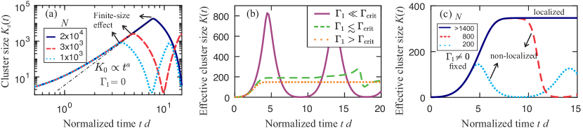
Figure 3: Effective cluster size of correlated spins $K(t)$ that defines the information scrambling predicted by our model. All simulations were performed for a three-dimensional system [$\delta=0.66$, see Eq. (26)]. (a) Cluster size dynamics $K_{0}(t)$ in the ideal case, i.e., without considering decoherence effects ($\Gamma_{1}=0$). Three different system sizes $N$ are shown in the legend. The cluster size grows as $K_{0}(t)\propto t^{a}$ until finite-size effects distort the evolution. All solutions are equivalent before the finite-size effects appear independently of the value of $N$. (b) Effective cluster size evolution $K(t)$, now including the decoherence effects ($\Gamma_{1}\neq 0$), using $N=10^{3}$. When $\Gamma_{1}\ll\Gamma_{\mathrm{crit}}$, the growth of $K(t)$ is delocalized until finite-size effects appear as in the case of $\Gamma_{1}=0$. Near the critical decoherence strength $\Gamma_{\mathrm{crit}}$, $K(t)$ tends to localize although it exhibits low-frequency oscillations. For $\Gamma_{1}>\Gamma_{\mathrm{crit}}$, $K(t)$ localizes indefinitely. (c) Finite-size effects on the observation of the localization dynamics. If $\Gamma_{1}\neq 0$, $K(t)$ will localize only if $N$ is large enough. If not, finite-size effects avoid the observation of the localization effects.

We then introduce the decoherence effects. For $\Gamma_{1}>0$, an initial power-law growth for the effective cluster size $K(t)$ is observed similarly to the case of $\Gamma_{1}=0$ [Fig. 3(b)]. However the exponent $a$ decreases slightly with increasing $\Gamma_{1}$. Again, at long times when finite-size effects are reached, oscillations are seen on the dynamics of $K(t)$. These oscillations decrease in frequency and amplitude as $\Gamma_{1}$ increases. When the decoherence strength $\Gamma_{1}$ increases above a critical value $\Gamma_{\mathrm{crit}}$, the effective cluster size $K(t)$ reaches a plateau which is maintained indefinitely in time. This plateau defines a localization size for the observed information scrambling determined by the effective cluster size. The predicted localization size is consistent with the experimental observations of Refs. [15, 9, 18]. If the system size of the model $N\rightarrow\infty$, we observe that $\Gamma_{\mathrm{crit}}\rightarrow 0$. This implies that considering power-law scalings for the leakage rates $\Gamma_{L}=\Gamma_{1}L^{\alpha}$ our model predicts that the effective cluster size dynamics localizes, provided that the system size $N$ is large enough if $\Gamma_{1}\neq 0$. We have also observed that localization effects are manifested even for slow-growing scaling laws as for $\Gamma_{L}\propto\log(L)$ or $L^{\alpha}$ with $\alpha<1$. Notice that, if the decoherence rate is independent of $L$, localization effects are not observed.

Figure 3(c) shows the dynamics of $K(t)$ for different values of $N$ for a given $\Gamma_{1}$, manifesting that localization effects are observed once $N$ is large enough. All the curves behave equally before finite-size effects are significant. Therefore if $N$ is large enough to manifest localization for a fixed rate $\Gamma_{1}>\Gamma_{\mathrm{crit}}$, the predicted curve for $K(t)$ is independent of $N$.

The effective cluster size $K(t)$ of Eq. (32) can be written in terms of the eigenbasis of $\Upsilon$ as

$$K(t)=\frac{\sum_{L}L|\sum_{i}c_{Li}\tilde{C}_{i}(t)|^{2}}{\sum_{L}|\sum_{i}c_{Li}\tilde{C}_{i}(t)|^{2}},$$ (35)

where the populations $C_{L}(t)$ are in terms of a linear combination of the evolution of $\tilde{C}_{i}(t)$, i.e., $C_{L}(t)=\sum_{i}c_{Li}\tilde{C}_{i}(t)$ with $c_{Li}$ the eigenvector coefficients. Using the solution for $\tilde{C}_{i}(t)$ determined from Eq. (34), we get

$$K(t) =\frac{\sum_{L}L\left|\sum c_{Li}\tilde{C}_{i}(0)e^{-t\lambda_{i}}\right|^{2}}{\sum_{L}|\sum_{i}c_{Li}\tilde{C}_{i}(0)e^{-t\lambda_{i}}|^{2}}.$$ (36)

The transition from a delocalized to a localized scrambling dynamics is evidenced in the behavior of the eigenvalues of $\Upsilon$ as a function of $\Gamma_{1}$ [Fig. 4(a) and (b)]. The eigenvalues $\left\{\lambda_{i}\right\}$ are purely imaginary for $\Gamma_{1}=0$, which implies the conservation of $\sum_{L}\left|C_{L}\right|^{2}$. However, if $\Gamma_{1}\neq 0$, the eigenvalues $\left\{\lambda_{i}\right\}$ are in general complex numbers $\lambda_{i}=\gamma_{i}+i\omega_{i}$, with real $\gamma_{i}$ and imaginary $\omega_{i}$ components. We consider the set $\left\{\lambda_{i}\right\}$ sorted by its real value, so as $\gamma_{i}\leq\gamma_{i+1}$. If $\Gamma_{1}<\Gamma_{\mathrm{crit}}$, then $\lambda_{1}=\lambda_{2}^{*}$, which implies that two different frequencies $\omega_{1}$ and $\omega_{2}=-\omega_{1}$ have the same decay constant $\gamma_{1}=\gamma_{2}$. Hence, in the long time limit, terms with decay constants $\gamma_{i}>\gamma_{1}$ become negligible and we obtain

$$K(t\rightarrow\infty)=\frac{\sum_{L}L\left|e^{-t\lambda_{1}}\sum_{i}c_{Li}\tilde{C}_{i}(0)e^{-t(\lambda_{i}-\lambda_{1})}\right|^{2}}{\sum_{L}|e^{-t\lambda_{1}}\sum_{i}c_{Li}\tilde{C}_{i}(0)e^{-t(\lambda_{i}-\lambda_{1})}|^{2}}$$

$$\sim\frac{\sum_{L}L\left|\left(c_{L1}\tilde{C}_{1}(0)+c_{L2}\tilde{C}_{2}(0)e^{-2it\omega_{1}}\right)\right|^{2}}{\sum_{L}\left|\left(c_{L1}\tilde{C}_{1}(0)+c_{L2}\tilde{C}_{2}(0)e^{-2it\omega_{1}}\right)\right|^{2}}.$$ (37)

This solution provides the oscillations observed for $K(t)$ due to the finite-size effects in Fig. 3.

If $\Gamma_{1}>\Gamma_{\mathrm{crit}}$, then $\lambda_{1}$ becomes a nondegenerate real eigenvalue ($\omega_{1}=0$ and $\gamma_{2}>\gamma_{1}$), implying that the effective cluster size $K(t)$ attain a localization value at long times

$$\lim_{t\rightarrow\infty}K(t)=K_{loc}=\frac{\sum_{L}L\left|c_{L1}\right|^{2}}{\sum_{L}\left|c_{L1}\right|^{2}}.$$ (38)

This demonstrates the existence of a localized regime for the observable information scrambling determined by $K(t)$ when $\Gamma_{1}>\Gamma_{\mathrm{crit}}$. Moreover, $K(t)$ converges always to the same stationary value, provided that the initial condition $\vec{C}(0)$ has a nonzero contribution of the $\tilde{C}_{1}$ eigenvector. This is because the coefficients $c_{L1}$ are independent of the initial condition $\vec{C}(0)$ in Eq. (38). Therefore, independently of the initial cluster size of correlated spins, the effective cluster size in the long time limit will converge to the same localization size consistently with experimental observations [15, 61, 80].

The delocalization-localization transition on the dynamical behavior of the information scrambling manifested by the evolution of $K(t)$, resembles the quantum dynamical phase transitions induced by decoherence effects [81, 82] that are connected with exceptional points ubiquitous in non-Hermitian Hamiltonians [83, 84, 85, 86].

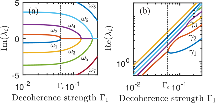
Figure 4: Eigenvalues of the transition rate operator $\Upsilon$ derived from our model. (a) Imaginary and (b) real parts of the eigenvalues ${\lambda_{i}}$ as a function of the decoherence strength $\Gamma_{1}$. We use a low number of $N=10$ to show clearer the functional behavior of the eigenfrequencies, but the qualitative behavior is analogous for larger $N$. For $\Gamma_{1}=0$, all the frequencies are pure imaginary numbers, therefore the global amplitude $\sum_{L}\left|C_{L}\right|^{2}$ of the system is strictly conserved. For $\Gamma_{1}\neq 0$, the solutions $\tilde{C}(t)$ become damped oscillations as ${\lambda_{i}}$ are complex numbers. There is a critical decoherence strength $\Gamma_{\mathrm{crit}}$ from which the smallest eigenvalue $\lambda_{1}$ becomes a real number. Localization effects can be deduced from the eigenspectrum: the existence of a nonoscillating, long-living solution $\tilde{C}_{1}(t)$ for $\Gamma_{1}>\Gamma_{\mathrm{crit}}$ implies that observed scrambling dynamics by $K(t)$ will eventually localize for long times.

VI Model vs. experiments: evaluation of the decoherent dynamics of information scrambling

VI.1 Information scrambling determined with NMR quantum simulations

We evaluate here the presented model as a framework to describe quantum information scrambling dynamics with imperfect echo experiments. We consider the MQC protocol based on imperfect time reversion echoes as described in Fig. 1(b), following the technique introduced in Refs. [15, 61]. In this experimental protocol, a controlled perturbation is introduced to the forward Hamiltonian $\mathcal{H}_{F}=(1-p)\mathcal{H}_{0}+p\Sigma$, where the nonreverted term $\Sigma$ is weighted by the dimensionless parameter $p$ using average Hamiltonian techniques that can control the perturbation strength $p$. This allows performing quantum simulations to evaluate the effect of nonreverted interactions that are inherent to any echo experiment.

We perform the experimental quantum simulations on a Bruker Avance III HD 9.4 T WB NMR spectrometer with a ${}^{1}\mathrm{H}$ resonance frequency of $\omega_{z}=400.15$ MHz. We consider the nuclear spins ${}^{1}\mathrm{H}$ of a powdered adamantane sample as the system, which constitutes a dipolar interacting many-body system of equivalent $1/2$ spins with a 3D spin-spin coupling network topology. The imperfect echo protocol of Fig. 1(b) is implemented using the perturbation Hamiltonian $\Sigma=\mathcal{H}_{dd}$ as the raw dipolar interaction of the system of Eq. (2). The perturbation Hamiltonian is introduced using the NMR sequence described in Refs. [15, 61]. This protocol provides a magnetization echo at the end of the sequence that is proportional to the fidelity function $f(\phi,t,p)$ of Eq. (16), from which we experimentally monitor the dynamics of the effective cluster size $K(t,p)$ based on Eq. (20) (see Fig. 5).

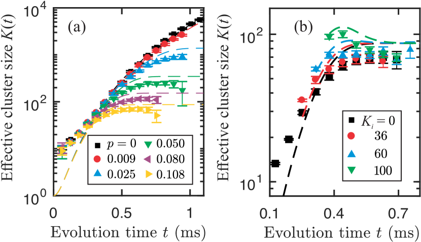
Figure 5: Quantum information scrambling determined from MQC experiments with imperfect time-reversals. (a) Effective cluster size $K(t)$ evolution determined from quantum simulations with solid-state NMR experiments on powdered adamantane for several perturbations strengths $p$ (symbols) with the perturbation Hamiltonian $\Sigma=\mathcal{H}_{dd}$. The corresponding predictions of our model are shown in dashed lines. (b) Experimentally determined effective cluster size $K(t)$ evolution starting from different initial conditions $K_{i}$ for $p=0.108$ (symbols). The effective cluster size $K(t)$ converges to a dynamical equilibrium determined by the localization size $K_{loc}$ independently of the initial cluster size $K_{i}$. The presented model correctly predicts the effective cluster size evolution towards the dynamical equilibrium (dashed lines).

We also calculate the instantaneous decay rate $\chi^{\prime}(t)=\frac{d\chi(t)}{dt}$ with $\chi=\log(f)$ of the echo fidelity $f(\phi,t,p)$, which is shown in Fig. 6(a).

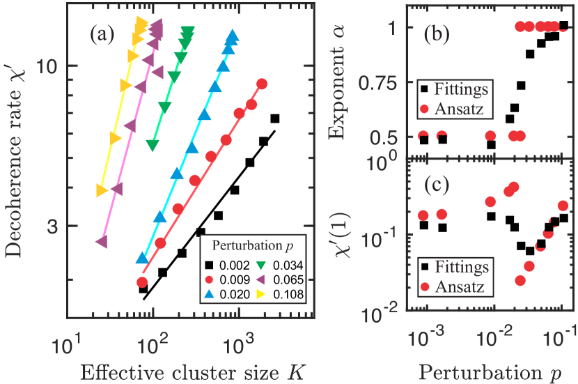
Figure 6: Decoherence scaling as a function of the perturbation strength. (a) Experimentally determined decoherence rates (symbols) and fitting curves (solid lines) $\chi^{\prime}(K)=\chi^{\prime}(1)K^{\alpha}$ for different perturbation strengths $p$. This power law behavior determines the decay rates $\Gamma(L)$ of the presented model. The scaling exponent $\alpha$ and the scaling factor $\chi^{\prime}(1)$ are shown in panels (b) and (c). Black squares are the fitting parameters of curves $\chi^{\prime}(K)$, and the red circles are the parameters determined by assuming the single-parameter ansatz of Eq. (39).

It is seen from the experiments that the decoherence rate scales with a power-law function $\chi^{\prime}(K)=\chi^{\prime}(1)K^{\alpha}$. This scaling behavior indicates the sensitivity of the controlled quantum dynamics to the perturbation as a function of the instantaneous effective cluster size $K$ [18].

For an unperturbed echo experiment ($p=0$), the cluster size $K_{0}(t)$ grows indefinitely following a power-law $K_{0}(t)\propto t^{4.3}$ up to the experimentally accessible timescales (black squares in Fig. 5). If the perturbation to the control Hamiltonian $p\neq 0$, the effective cluster size $K(t)$ growth is reduced. The decay rate $\chi^{\prime}(K)$ and its power-law exponent $\alpha$ increase with the perturbation strength $p$ (Fig. 6). As seen in Fig. 5(a), $K(t)$ reaches a localization value $K_{loc}$ that remains constant in time for large perturbations $p>0.02$ [15, 9]. This localization size reduces by increasing the perturbation strength $p$ consistently with the predictions of Sec. V.

The experimental results evidence that $K_{loc}$ is determined by a dynamical equilibrium of $K(t)$ that converges to the same stationary value, independently of the initial cluster size [15, 61, 80]. Figure 5(b) shows a series of experiments following the protocol implemented in Refs. [15, 61, 80]. Here, an initial cluster size of correlated spins $K_{i}$ is prepared by an unperturbed evolution with the propagator $U_{0}=e^{-it_{ini}\mathcal{H}_{0}}$, where $t_{ini}$ is the initialization time required for preparing the initial cluster size. Then, the cluster size $K_{i}$ is used as the initial information state for the perturbed evolution $U_{p}=e^{-it[(1-p)\mathcal{H}_{0}+p\Sigma]}$. As shown in Refs. [15, 61, 80], the cluster size converges to a localization size $K_{loc}(p)$ independently of the initial value of $K_{i}$.

VI.2 Quantitative evaluation of the decoherent model for the information scrambling dynamics

We perform here a quantitative comparison between the predictions of our model and the experimental results of the information scrambling dynamics in imperfect echo experiments. We determine the parameters $d$ and $\delta$ of Eq. (26) to reproduce the cluster size dynamics at $p=0$ shown in Fig. 5(a). We observe from the experimental data that the cluster size is $K_{0}(t)\approx(7.41\,\frac{1}{\text{ms}}\,t)^{4.2}$. We found that the power law exponent $a=4.2$ is obtained if $\delta=0.78$. This value is slightly larger than the expected $1-1/D=0.66$ for a three-dimensional system as in our case, according to the original Levy-Gleason model. This result is consistent with a cluster size that keeps growing for a long time, at a rate that is faster than in normal diffusion [80]. This might be related with a “super-diffusion” mechanism due to the complex long-range nature of the dipolar interaction in our system [87, 88]. Setting $d=13$kHz defined by the width of the resonance line of adamantane, we obtain an excellent agreement with the experimental evolution of $K_{0}(t)$ as shown by black dashed lines in Fig. 5(a).

To predict the evolution of the effective cluster size $K(t)$ for every perturbation strength $p$, we need to define the decay rates $\Gamma(L)$ in Eq. (30) for the average $L$-spin operators $P_{L}$. The experimentally observed decay rates $\chi^{\prime}(K)=\chi^{\prime}(1)K^{\alpha}$ [Fig. 6 (a)] of the fidelity $f$ have a power law dependence on the instantaneous cluster size $K(t)$ with a power law exponent $\alpha$ and proportionally constant $\chi^{\prime}(1)$ that depend on the perturbation strength [black squares in Fig. 6 (b) and (c) respectively]. We assume that these decoherence rates determine the decay rates of the model as $\Gamma(L)=\chi^{\prime}(L)$ for each perturbation strength. The exponent $\alpha$ presents a transition as a function of $p$, between a low-scaling regimen with $\alpha\sim 0.5$ for weak perturbations and a high-scaling regimen with $\alpha\sim 1$ for large perturbations [18].

We calculate then $K(t)$, using a system size $N=2\times 10^{4}$ large enough to avoid finite-size effects on the experimentally accessible temporal scales of Fig. 5(a). We compare the experimental results for $K(t)$ in Fig. 5(a) with their predictions for several perturbation strengths. The calculated $K(t)$ correctly predicts its time evolution and the achieved localization size $K_{loc}$ for large $p$, although $K_{loc}$ is slightly overestimated in all cases. The model predicts with high accuracy the cluster size growth for the long-time behavior of the weakest perturbation strengths.

Our model also quantitatively predicts well the dynamical equilibrium localization size $K_{loc}$ predicted in subsection VI.1 as show in Fig. 5(b), for the perturbation strength $p=0.108$. The dynamical equilibrium value for the localization size $K_{loc}$ is determined from Eq. (38) as the eigenvector matrix $c_{Lk}$ is independent of the initial condition.

Figure 7 shows with black squares the prediction for the localization size $K_{loc}$ as a function of the perturbation strength $p$ compared with the ones determined from the experimental data (yellow diamonds scatters).

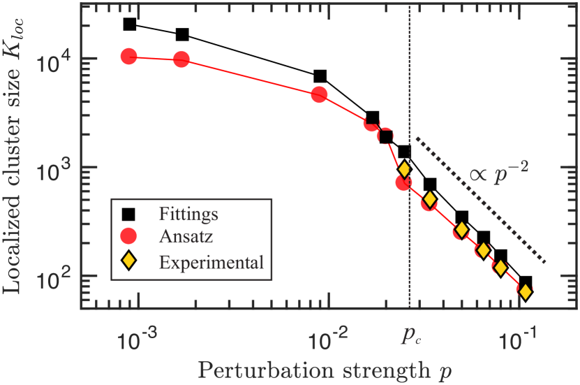
Figure 7: Localization cluster size $K_{loc}$ as a function of the perturbation strength for the perturbation Hamiltonian $\Sigma=\mathcal{H}_{dd}$. Yellow diamonds show the experimentally determined localization sizes only for the largest perturbation strengths where localization effects are observed. We observe a power-law dependence $K_{loc}\propto p^{-2}$ shown with a dotted line as a guide to the eye. The black squares are the localization size predicted by our model for every studied perturbation using the measured parameters $\chi^{\prime}(1)$ and $\alpha$ from the black symbols in Fig. 6 (b) and (c). The red circles are the predicted localization size determined from our model assuming the single-parameter ansatz of Eq. (39) using the experimentally determined parameters $s,\nu,\alpha_{0}$, and $\alpha_{\infty}$. The predicted localization size $K_{loc}$ exhibits two different scaling regimes as a function of the perturbation strength, for weak and strong perturbations. The determined critical perturbation $p_{c}$, where this transition occurs, is shown with a vertical dashed line.

We determined $K_{loc}$ from Eq. (38) which only depends on the eigenvector coefficients $c_{L1}$ associated to the smallest eigenvalue $\lambda_{1}$. The calculation of a single eigenvector can be performed in shorter times compared with solving the full system dynamics, allowing us to calculate $K_{loc}$ for systems with $N=2\times 10^{5}$. The computed values of $K_{loc}$ evidence two different regimes. For large perturbations ($p>0.025$) our model predicts a scaling for the localization size $K_{loc}(p)\propto p^{-2}$. For weak perturbations ($p<0.025$), we observe a weaker dependence of the localization size as a function of the perturbation that can be described approximately by $K_{loc}(p)\propto p^{-0.5}$. This transition is consistent with the transition on the decoherence scaling exponent $\alpha$ shown in Fig. 6(b). Experimental evidence of localization effects is only observed for $p>0.026$, therefore only these experimental data are shown in Fig. 7. Within this perturbation regime the experimental values exhibit a functional dependence $K_{loc}(p)\propto p^{-2}$ consistently with our predictions from the model. We do not observe experimental evidence of localization effects for weaker perturbations within the accessible time which is limited by the decoherence decay of the NMR signal. The largest cluster sizes observed experimentally for the weak perturbations are always lower than the predicted localization sizes.

In a previous work [18], we showed experimental evidence that the scaling behavior of decoherence as a function of the cluster size is consistent with the single-parameter ansatz for the asymptotic functional dependence at long times

$$\chi^{\prime}(p,K)\sim\begin{cases}(p_{c}-p)^{s}K^{\alpha_{0}}&p<p_{c}\\ (p-p_{c})^{-2\nu}K^{\alpha_{\infty}}&p>p_{c},\end{cases}$$ (39)

where we obtained the critical exponents $s=(-0.911\pm 0.004$) and $\nu=(-0.57\pm 0.03)$. The scaling exponents are $\alpha_{\infty}=0.96\pm 0.02$, near to a linear scaling, and $\alpha_{0}=(0.48\pm 0.03)$. The determined critical perturbation is $p_{c}=(0.026\pm 0.006)$. Due to the finite evolution time of the experimental data, the transition from one regime to another is smooth (see Fig. 6). The experimental data give a smooth functional behavior also for the decay rate $\Gamma(K)=\chi^{\prime}(K)$ that we introduced in our model [black squares in Fig. 6(b,c)]. To further evaluate the consistency of the scaling behavior determined by Eq. (39) and extrapolate its predicted behavior for the weak perturbations where we do not have experimental data, we assume this functional behavior for $\Gamma(K)=\chi^{\prime}(K)$ using the extracted parameters $s,\nu,\alpha_{0}$ and $\alpha_{\infty}$. Figure 7 shows with red circles the prediction for the localization size $K_{loc}$ as a function of the perturbation strength $p$. The localization size $K_{loc}$ determined from Eq. (38) now fit better the experimental data for the strong perturbations ($p>0.025$). Again for weak perturbations ($p<0.025$), we observe a weaker dependence of the localization size as a function of the perturbation strength. However, our model now predicts a finite localization size when $p\rightarrow 0$.

Both assumptions for $\Gamma(K)=\chi^{\prime}(K)$ manifest different scaling laws for $K_{loc}$ comparing the weak and strong perturbation regimes. For weak perturbations, it seems from the predicted curves that there might exist a limiting value for $K_{loc}$ for $p\rightarrow 0$. Further experimental designs need to be implemented to verify if the experimental behavior matches these predictions, but we expect that this limiting value is due to intrinsic perturbations on the experimental implementation that are not accounted for in our microscopic model described in Sec. II and in Refs. [9, 18].

VII Conclusion and discussions

We developed a model for studying the quantum information scrambling dynamics based on active spins clusters measured via out-of-time-order correlators determined from Loschmidt echoes combined with multiple quantum coherences experiments. Experimental implementations ubiquitously contain imperfections in the quantum operations that lead to the presence of nonreversed interactions in the LE procedure for measuring the OTOC. Based on considering an imperfect experimental protocol, we derived expressions for OTOC functions connected with the effective number of correlated spins that are active on quantum superpositions generated by coherence transfers of a local information, that survived the perturbation effects. Decoherence effects induced by the time-reversal imperfection arise naturally by the derived OTOCs as a leakage of the ideal unitary dynamics. The derived OTOCs quantify the observable degree of scrambling of information based on an inner product between the ideal and the perturbed scrambling dynamics. The main prediction of our model is the existence of localization effects on the measurable information scrambling that bound the effective cluster size $K(t)$ where the ideal information was propagated. We also found that whether the initial information on $K(0)$ is local or not, the dynamics of the effective cluster size $K(t)$ tends to a dynamical equilibrium value $K_{loc}$. Our predictions were contrasted with quantum simulations performed with NMR experiments on a solid-state adamantane sample, showing excellent quantitative agreement with the experimental observations.

Levy and Gleason originally proposed a model to describe the dynamics of the spin cluster of correlated spins in MQC experiments in solid-state samples. The model was based on simplifying the spin quantum dynamics to a phenomenological equation depending on two physical parameters: the mean value of the spin-spin interactions and the number of dimensions of the system. It correctly described how the number of correlated spins grows in NMR solid-state experiments with only these parameters. Our work revisits this model and adapts it to treat information scrambling. We also introduced a decoherence process induced by imperfection on the experimental implementations into the model. The decoherence process is described by a leakage rate that depends on the number of active spins involved in the states that describe the dynamics of the system. Determining this rate from experimental data, we obtained accurate predictions of the cluster size growth as a function of time and the localization values that were experimentally observed. Our results indicate that quantum information scrambling dynamics and its localization effects due to perturbations are phenomena that can be predicted in terms of few physical parameters by the presented model.

Treating many-body dynamics with exact numerical solutions is not possible with present technology. Therefore, the results shown in this work provide a framework for describing the quantum information scrambling dynamics of many-body systems determined from experiments affected by nonunitary decays, either by imperfections on the control or from interaction with external degrees of freedom. In this article, we have focused on modeling the dynamics of quantum information based on OTOC functions that give the cluster size of correlated spins generated by the scrambling dynamics. However, the model building block is based on finding the density matrix evolution of the system by solving the Liouville-von Neumann equation reduced to the average operator of the active spins in the dynamics. Therefore, one can envisage that the approach can be adapted to study the dynamic behavior of relevant physical quantities such as other types of correlations in the presence of decoherence effects [89, 90, 91, 92, 93]. The framework presented here can be a useful tool to predict the quantum information dynamics in large quantum systems and address the effect of imperfections on the control Hamiltonian that drives the quantum evolutions.

Appendix A Quantum information scrambling as the cluster size of active spins

We here demonstrate that the norm of the commutator $\left[I_{z},\sigma^{0}(t)\right]$ quantifies the average number of active spins in the operator $\sigma^{0}(t)=U_{0}(t)\sigma U_{0}^{\dagger}(t)$ with $\sigma$ an arbitrary operator of the system. Then, when the operator $\sigma=I_{z}$, the following demonstration relates the cluster size of correlated spins of Eq. (13) and the OTO commutator of Eq. (11). We first calculate the commutator $\left[I_{z},\sigma^{0}(t)\right]$ of the OTOC expression of Eq. (11). We find that $\left[I_{z},\sigma^{0}(t)\right]=\sum_{j}^{N}\sum_{\vec{u}}C_{\vec{u}}^{0}(t)[I_{z}^{j},P_{\vec{u}}]$, where we used that $\sigma^{0}(t)=\sum_{\vec{u}}C_{\vec{u}}^{0}(t)P_{\vec{u}}$ and $I_{z}=\sum_{j}^{N}I_{z}^{j}$. The operator $I_{z}$ is a mixture of local spin operators $I_{z}^{j}$,

$$I_{z}^{j}=\underbrace{\mathbb{I}\otimes...}_{j-1}\otimes\underbrace{I_{z}^{(1)}}_{j}\otimes\underbrace{...\otimes\mathbb{I}}_{N-j}.$$ (40)

The operators $P_{\vec{u}}$ are the elements of the orthonormal product basis $\left\{\left(\sqrt{2}\right)^{N}\bigotimes_{k=1}^{N}I_{u_{k}}^{{}^{(1)}}\right\}$, where the coefficients of the vector $\vec{u}$ are $u_{i}\in\{x,y,z,0\}$ (zero for identity operator $I_{0}=\mathbb{I})$. By using the following property of the Kronecker product

$$[A\otimes B,C\otimes D]=[A,C]\otimes BD+CA\otimes[B,D]$$ (41)

and the expression for $I_{z}^{j}$ of Eq. (40), the commutator $[I_{z}^{j},P_{\vec{u}}]$ is

$$[I_{z}^{j},P_{\vec{u}}] =\left(\sqrt{2}\right)^{N}\underbrace{I_{u_{1}}\otimes...}_{j-1}\otimes[I_{z}^{(1)},I_{u_{j}}]\otimes\underbrace{...\otimes I_{u_{N}}}_{N-j}$$

$$=\begin{cases}iP_{\vec{u}^{\prime}(j)}&\text{$\mathrm{if}$\,$u_{j}=x$}\\ -iP_{\vec{u}^{\prime}(j)}&\mathrm{if}\,u_{j}=y\\ 0&\mathrm{if}\,u_{j}=0,z\end{cases}.$$ (42)

The operator $P_{\vec{u^{\prime}}(j)}$ belongs to the product basis $\{P_{\vec{u}}\}$, where the vector $\vec{u}^{\prime}(j)$ is a vector identical to $\vec{u}$, except for the $j$-th element (e.g. if $u_{j}=x$ then $u^{\prime}(j)_{j}=y$ and vice versa). We have used that $[I_{z}^{(1)},I_{x}^{(1)}]=iI_{y}^{(1)}$, $[I_{z}^{(1)},I_{y}^{(1)}]=-iI_{x}^{(1)}$ and $[I_{z}^{(1)},I_{z}^{(1)}]=[I_{z}^{(1)},\mathbb{I}]=0$. This means that if $[I_{z}^{j},P_{\vec{u}}]\neq 0$, then $[I_{z}^{j},P_{\vec{u}}]$ is proportional to the other element $P_{\vec{u^{\prime}}(j)}$ of the product basis $\{P_{\vec{u}}\}$. The sign of $[I_{z}^{j},P_{\vec{u}}]$ depends on whether $u_{j}=x$ $(+)$ or $u_{j}=y$ $(-).$

We then find that the commutator

$$[I_{z},P_{\vec{u}}]=\sum_{j=1}^{N}[I_{z}^{j},P_{\vec{u}}]=\sum_{j\in\mathcal{A}(\vec{u})}\pm iP_{\vec{u}^{\prime}(j)},$$

where $\mathcal{A}(\vec{u})$ is the set of indeces $\{j\}$ corresponding to active spins in $\vec{u}$, that is, those which satisfy $u_{j}=x,y$. The set $\mathcal{A}(\vec{u})$ has $L(\vec{u})$ elements, where $L(\vec{u})$ is the number of elements $u_{j}$ equal to $x$ and $y$, which implies that $[I_{z},P_{\vec{u}}]$ has $L(\vec{u})$ nonzero terms $\pm iP_{\vec{u}^{\prime}(j)}$. The resulting expression for the OTOC and therefore for cluster size $K_{0}(t)$ is then

$$K_{0}(t)=\mathrm{Tr}\left\{[I_{z},\sigma^{0}(t)][I_{z},\sigma^{0}(t)]{}^{\dagger}\right\}\\ =\sum_{\vec{u},\vec{v}}C_{\vec{u}}^{0}C_{\vec{v}}^{0*}\times\\ \times\sum_{i\in\mathcal{A}(\vec{u})}\sum_{j\in\mathcal{A}(\vec{v})}\mathrm{Tr}\left[\left(\pm iP_{\vec{u}^{\prime}(i)}\right)\left(\pm iP_{\vec{v}^{\prime}(j)}\right)^{\dagger}\right].$$ (43)

Finally, we prove that the factor of the previous equation is equal to the function $\mathcal{L}(\vec{u},\vec{v})$ introduced in Eq. (14)

$$\mathcal{L}(\vec{u},\vec{v})=\sum_{i\in\mathcal{A}(\vec{u})}\sum_{j\in\mathcal{A}(\vec{v})}\mathrm{Tr}\left[\left(\pm iP_{\vec{u}^{\prime}(i)}\right)\left(\pm iP_{\vec{v}^{\prime}(j)}\right)^{\dagger}\right].$$ (44)

To prove this, we divide the demonstration into five different propositions as we discuss below. We introduce the notation $h_{0z}(\vec{u},\vec{v})$ for the Hamming distance between $\vec{u}$ and $\vec{v}$ considering only the elements zero,$z$, and $h_{xy}(\vec{u},\vec{v})$ for the Hamming distance between $\vec{u}$ and $\vec{v}$ considering only the elements $x,y$. In Propositions 1 and 2, we deduce the necessary conditions that $\vec{u}$ and $\vec{v}$ must satisfy for obtaining $\mathcal{L}(\vec{u},\vec{v})\neq 0$. Then, Propositions 3, 4 and 5 provide the values of $\mathcal{L}(\vec{u},\vec{v})$ when the conditions deduced in Propositions 1 and 2 are satisfied.

Proposition 1

If $\mathcal{L}(\vec{u},\vec{v})\neq 0$, then $h_{0z}(\vec{u},\vec{v})=0$.

Proof:

Since $\{P_{\vec{u}}\}$ is an orthonormal base $\mathrm{Tr}\left(P_{\vec{u}^{\prime}(i)}P_{\vec{v}^{\prime}(j)}\right)=\delta_{\vec{u}^{\prime}(i),\vec{v}^{\prime}(j)}$, to obtain $\mathcal{L}(\vec{u},\vec{v})\neq 0$, there must be states $\vec{u}^{\prime}(i)=\vec{v}^{\prime}(j)$ for some $i\in\mathcal{A}(\vec{u})$, $j\in\mathcal{A}(\vec{v})$. Since the vectors $\vec{u}^{\prime}(i)$ and $\vec{v}^{\prime}(j)$ are identical to $\vec{u}$ and $\vec{v}$ respectively, in those elements that are equal to $z,$zero, it is necessary that $u_{l}=v_{l}$ if $l=0,z$ for $\vec{u}^{\prime}(i)=\vec{v}^{\prime}(j)$ to exist. Therefore, the Hamming distance $h_{0z}(\vec{u},\vec{v})=0$.

$\blacksquare$

Proposition 2

If $\mathcal{L}(\vec{u},\vec{v})\neq 0$, then $h_{xy}(\vec{u},\vec{v})=0$ or $2$.

Proof:

Again, to obtain $\mathcal{L}(\vec{u},\vec{v})\neq 0$, there must be states $\vec{u}^{\prime}(i)=\vec{v}^{\prime}(j)$ for some $i\in\mathcal{A}(\vec{u})$, $j\in\mathcal{A}(\vec{v})$. We prove Proposition 2 in two steps.

(i) We can see first that if $\mathcal{L}(\vec{u},\vec{v})\neq 0$, $h_{xy}(\vec{u},\vec{v})\leq 2$. From the definition of the vectors $\vec{u^{\prime}}(i)$, we know that $\vec{u^{\prime}}(i)$ only differs from $\vec{u}$ in the $i$-th element, and that $u_{i}$ must be $x$ or $y$. We thus deduce that $h_{xy}\left(\vec{u},\vec{u}^{\prime}(i)\right)=h_{xy}\left(\vec{v},\vec{v}^{\prime}(j)\right)=1$, for every $i\in\mathcal{A}(\vec{u})$, $j\in\mathcal{A}(\vec{v})$. If $\vec{u}^{\prime}(i)=\vec{v}^{\prime}(j)$ for some $i,j$, we then deduce from the triangle inequality that

$$h_{xy}(\vec{u},\vec{v}) \leq h_{xy}\left(\vec{u},\vec{u}^{\prime}(i)\right)+h_{xy}\left(\vec{v},\vec{u}^{\prime}(i)\right)$$

$$=h_{xy}\left(\vec{u},\vec{u}^{\prime}(i)\right)+h_{xy}\left(\vec{v},\vec{v}^{\prime}(j)\right)$$

$$=2.$$ (45)

(ii) We can also see that $h_{xy}(\vec{u},\vec{v})\neq 1$. Let us suppose that $h_{xy}(\vec{u},\vec{v})=1$, then there is a unique index $l$ such that $u_{l}\neq v_{l}$. Therefore $\vec{v}=\vec{u}^{\prime}(l)$, and then it is impossible to find $\vec{v}^{\prime}(j)$ such that $\vec{u}^{\prime}(l)=\vec{v}^{\prime}(j)$, because $\vec{v}^{\prime}(j)\neq\vec{v}=\vec{u}^{\prime}(l)$. If we consider $\vec{u}^{\prime}(i)$ (with $i\neq l$) then $h_{xy}\left(\vec{u}^{\prime}(i),\vec{v}\right)=2$ and again it is impossible to find $\vec{v}^{\prime}(j)$ such that $\vec{u}^{\prime}(i)=\vec{v}^{\prime}(j)$. We have proven that if $h_{xy}(\vec{u},\vec{v})=1$ then $\mathcal{L}(\vec{u},\vec{v})=0$. Therefore, if $\mathcal{L}(\vec{u},\vec{v})\neq 0$, then $h_{xy}(\vec{u},\vec{v})\neq 1$. Therefore, if $\mathcal{L}(\vec{u},\vec{v})\neq 0$, $h_{xy}(\vec{u},\vec{v})=0$ or $h_{xy}(\vec{u},\vec{v})=2$.

$\blacksquare$

Proposition 3

$\mathcal{L}(\vec{u},\vec{u})=L(\vec{u})$, where $L(\vec{u})$ is the number of elements in $\vec{u}$ that are equal to $x,y$. Notice that in this case when $\vec{u}=\vec{v}$, the Hamming distances are $h_{xy}(\vec{u},\vec{v})=0$ and $h_{0z}(\vec{u},\vec{v})=0$.

Proof:

Since $\{P_{\vec{u}}\}$ is an orthonormal basis, $\mathrm{Tr}\left(P_{\vec{u}^{\prime}(i)}P_{\vec{v}^{\prime}(j)}\right)=\delta_{\vec{u}^{\prime}(i),\vec{v}^{\prime}(j)}$. As the number of elements in $\mathcal{A}(\vec{u})$ is $L(\vec{u})$, we get

$$\mathcal{L}(\vec{u},\vec{u}) =\sum_{i\in\mathcal{A}(\vec{u})}\sum_{j\in\mathcal{A}(\vec{u})}\mathrm{Tr}\left[\left(\pm iP_{\vec{u}^{\prime}(i)}\right)\left(\pm iP_{\vec{u}^{\prime}(j)}\right)^{\dagger}\right]$$

$$=-i^{2}\sum_{j\in\mathcal{A}(\vec{u})}1$$

$$=L(\vec{u}).$$ (46)

$\blacksquare$

Proposition 4

If $h_{xy}(\vec{u},\vec{v})=2$, $h_{0z}(\vec{u},\vec{v})=0$ and $\vec{u}$ is not a permutation of $\vec{v}$, i.e., $\vec{u}\neq\Pi(\vec{v})$, then $\mathcal{L}(\vec{u},\vec{v})=-2$.

Proof:

Since $h_{xy}(\vec{u},\vec{v})=2$ and $h_{0z}(\vec{u},\vec{v})=0$, there are only two indices $l_{1}$ and $l_{2}$ for which $u_{l_{1}}\neq v_{l_{1}}$ and $u_{l_{2}}\neq v_{l_{2}}$. Since $l_{1},l_{2}\in\{x,y\}$ and $\vec{u}\neq\Pi(\vec{v})$, there must be the following conditions $u_{l_{1}}=x$, $u_{l_{2}}=x$ and $v_{l_{1}}=y$ , $v_{l_{2}}=y$, or vice versa that are equivalent to exchange $\vec{u}$ and $\vec{v}$. Then, we have that $\vec{u}^{\prime}(l_{1})=\vec{v}^{\prime}(l_{2})$ and $\vec{u}^{\prime}(l_{2})=\vec{v}^{\prime}(l_{1})$. These are the only two terms different from zero in Eq. (44). If $u_{l_{1}}=u_{l_{2}}=x$, then the operators $P_{\vec{u}^{\prime}(l_{1})}$ and $P_{\vec{u}^{\prime}(l_{2})}$ have a multiplicative factor $i$. Analogously, since $v_{l_{1}}=v_{l_{2}}=y$ , then the operators $P_{\vec{v}^{\prime}(l_{1})}$ and $P_{\vec{v}^{\prime}(l_{2})}$ have a multiplicative factor $-i$. Therefore, the operator products $P_{\vec{u}^{\prime}(l_{1})}P_{\vec{v}^{\prime}(l_{2})}$ and $P_{\vec{u}^{\prime}(l_{2})}P_{\vec{v}^{\prime}(l_{1})}$ are proportional to $i^{2}=-1$, and the function $\mathcal{L}(\vec{u},\vec{v})$ is

$$\sum_{i\in\mathcal{A}(\vec{u})}\sum_{j\in\mathcal{A}(\vec{v})}\mathrm{Tr}\left[\left(\pm iP_{\vec{u}^{\prime}(i)}\right)\left(\pm iP_{\vec{v}^{\prime}(j)}\right)^{\dagger}\right]=\\ =i(-i)^{*}\mathrm{Tr}\left(P_{\vec{u}^{\prime}(l_{1})}P_{\vec{v}^{\prime}(l_{2})}\right)+\\ +(-i)^{*}i\mathrm{Tr}\left(P_{\vec{v}^{\prime}(l_{1})}P_{\vec{u}^{\prime}(l_{2})}\right)\\ =-2.$$ (47)

$\blacksquare$

Proposition 5

If $h_{xy}(\vec{u},\vec{v})=2$, $h_{0z}(\vec{u},\vec{v})=0$ and $\vec{u}$ is a permutation of $\vec{v}$, i.e. $\vec{u}=\Pi(\vec{v})$, then $\mathcal{L}(\vec{u},\vec{v})=2$.

Proof:

Since $h_{xy}(\vec{u},\vec{v})=2$ and $h_{0z}(\vec{u},\vec{v})=0$, there are only two indices $l_{1}$ and $l_{2}$ for which $u_{l_{1}}\neq v_{l_{1}}$ and $u_{l_{2}}\neq v_{l_{2}}$. Since $l_{1},l_{2}\in\{x,y\}$ and $\vec{u}=\Pi(\vec{v})$, it must hold that $u_{l_{1}}=x$ , $u_{l_{2}}=y$ and $v_{l_{1}}=y$ , $v_{l_{2}}=x$. Then, we have that $\vec{u}^{\prime}(l_{1})=\vec{v}^{\prime}(l_{2})$ and $\vec{u}^{\prime}(l_{2})=\vec{v}^{\prime}(l_{1})$. These are the only two terms different from zero in Eq. (44). Since $u_{l_{1}}=v_{l_{2}}=x$, then the operators $P_{\vec{u}^{\prime}(l_{1})}$ and $P_{\vec{v}^{\prime}(l_{2})}$ have a multiplicative factor $i$. Analogously, since $v_{l_{1}}=u_{l_{2}}=y$ , then the operators $P_{\vec{v}^{\prime}(l_{1})}$ and $P_{\vec{u}^{\prime}(l_{2})}$ have a multiplicative factor $-i$. Therefore, the operator products $P_{\vec{u}^{\prime}(l_{1})}P_{\vec{v}^{\prime}(l_{2})}$ and $P_{\vec{u}^{\prime}(l_{2})}P_{\vec{v}^{\prime}(l_{1})}$ are proportional to $-i^{2}=1$, and the function $\mathcal{L}(\vec{u},\vec{v})$ is

$$\sum_{i\in\mathcal{A}(\vec{u})}\sum_{j\in\mathcal{A}(\vec{v})}\mathrm{Tr}\left[\left(\pm iP_{\vec{u}^{\prime}(i)}\right)\left(\pm iP_{\vec{v}^{\prime}(j)}\right)^{\dagger}\right]=$$

$$=i\cdot(i)^{*}\mathrm{Tr}\left(P_{\vec{u}^{\prime}(l_{1})}P_{\vec{v}^{\prime}(l_{2})}\right)+(i)^{*}i\mathrm{Tr}\left(P_{\vec{v}^{\prime}(l_{1})}P_{\vec{u}^{\prime}(l_{2})}\right)$$

$$=2.$$ (48)

$\blacksquare$

These five propositions thus demonstrate the expression of Eq. (14) in the main text for the function $\mathcal{L}(\vec{u},\vec{v})$.

For the perturbed case the effective cluster size $K(t)$ of Eq. (22) is derived directly from the previous demonstration. But, we now write $\sigma^{0}(t)=\sum_{\vec{u}}C_{\vec{u}}^{0}(t)P_{\vec{u}}$ and $\sigma(t)=\sum_{\vec{u}}C_{\vec{u}}(t)P_{\vec{u}}$, and then

$$K(t)=\mathrm{Tr}\left[[I_{z},\sigma^{0}(t)][I_{z},\sigma(t)]{}^{\dagger}\right]$$

$$=\sum_{\vec{u},\vec{v}}C_{\vec{u}}^{0}(t)C_{\vec{v}}^{*}(t)\left\{\sum_{i\in\mathcal{A}(\vec{u})}\sum_{j\in\mathcal{A}(\vec{v})}\mathrm{Tr}\left[\left(\pm iP_{\vec{u}^{\prime}(i)}\right)\left(\pm iP_{\vec{v}^{\prime}(j)}\right)^{\dagger}\right]\right\},$$ (49)

where the function $\mathcal{L}(\vec{u},\vec{v})=\sum_{i\in\mathcal{A}(\vec{u})}\sum_{j\in\mathcal{A}(\vec{v})}\mathrm{Tr}\left[\left(\pm iP_{\vec{u}^{\prime}(i)}\right)\cdot\left(\pm iP_{\vec{v}^{\prime}(j)}\right)^{\dagger}\right]$ is the same as Eq. (14) for the nonperturbed case. The expression for $K(t)$ of Eq. (22) is obtained when $\sigma^{0}(t)=I_{z}^{0}(t)$ and $\sigma(t)=I_{z}(t)$.

References

- Sekino and Susskind [2008] Y. Sekino and L. Susskind, Fast scramblers, J. High Energy Phys. 2008, 065.
- Lashkari et al. [2013] N. Lashkari, D. Stanford, M. Hastings, T. Osborne, and P. Hayden, Towards the fast scrambling conjecture, J. High Energy Phys. 2013, 22.
- Martinez et al. [2016] E. A. Martinez, C. A. Muschik, P. Schindler, D. Nigg, A. Erhard, M. Heyl, P. Hauke, M. Dalmonte, T. Monz, P. Zoller, and R. Blatt, Real-time dynamics of lattice gauge theories with a few-qubit quantum computer, Nature 534, 516 (2016).
- Friis et al. [2018] N. Friis, O. Marty, C. Maier, C. Hempel, M. Holzäpfel, P. Jurcevic, M. B. Plenio, M. Huber, C. Roos, R. Blatt, and B. Lanyon, Observation of Entangled States of a Fully Controlled 20-Qubit System, Phys. Rev. X 8, 21012 (2018).
- Swingle [2018] B. Swingle, Unscrambling the physics of out-of-time-order correlators, Nat. Phys. 14, 988 (2018).
- Lewis-Swan et al. [2019] R. J. Lewis-Swan, A. Safavi-Naini, A. M. Kaufman, and A. M. Rey, Dynamics of quantum information, Nat. Rev. Phys. 1, 627 (2019).
- Eisert et al. [2015] J. Eisert, M. Friesdorf, and C. Gogolin, Quantum many-body systems out of equilibrium, Nat. Phys. 11, 124 (2015).
- Abanin et al. [2019] D. A. Abanin, E. Altman, I. Bloch, and M. Serbyn, Colloquium: Many-body localization, thermalization, and entanglement, Rev. Mod. Phys. 91, 21001 (2019).
- Álvarez et al. [2015] G. A. Álvarez, D. Suter, and R. Kaiser, Localization-delocalization transition in the dynamics of dipolar-coupled nuclear spins, Science 349, 846 (2015).
- Schweigler et al. [2017] T. Schweigler, V. Kasper, S. Erne, I. Mazets, B. Rauer, F. Cataldini, T. Langen, T. Gasenzer, J. Berges, and J. Schmiedmayer, Experimental characterization of a quantum many-body system via higher-order correlations, Nature 545, 323 (2017).
- Lukin et al. [2019] A. Lukin, M. Rispoli, R. Schittko, M. E. Tai, A. M. Kaufman, S. Choi, V. Khemani, J. Léonard, and M. Greiner, Probing entanglement in a many-body-localized system, Science 364, 256 (2019).
- Landsman et al. [2019] K. A. Landsman, C. Figgatt, T. Schuster, N. M. Linke, B. Yoshida, N. Y. Yao, and C. Monroe, Verified quantum information scrambling, Nature 567, 61 (2019).
- Brydges et al. [2019] T. Brydges, A. Elben, P. Jurcevic, B. Vermersch, C. Maier, B. P. Lanyon, P. Zoller, R. Blatt, and C. F. Roos, Probing Rényi entanglement entropy via randomized measurements, Science 364, 260 (2019).
- Krojanski and Suter [2004] H. G. Krojanski and D. Suter, Scaling of Decoherence in Wide NMR Quantum Registers, Phys. Rev. Lett. 93, 090501 (2004).
- Álvarez and Suter [2010] G. A. Álvarez and D. Suter, NMR quantum simulation of localization effects induced by decoherence, Phys. Rev. Lett. 104, 230403 (2010).
- Sánchez et al. [2014] C. M. Sánchez, R. H. Acosta, P. R. Levstein, H. M. Pastawski, and A. K. Chattah, Clustering and decoherence of correlated spins under double quantum dynamics, Phys. Rev. A 90, 042122 (2014).
- Niknam et al. [2020] M. Niknam, L. F. Santos, and D. G. Cory, Sensitivity of quantum information to environment perturbations measured with a nonlocal out-of-time-order correlation function, Phys. Rev. Research 2, 13200 (2020).
- Domínguez et al. [2021] F. D. Domínguez, M. C. Rodríguez, R. Kaiser, D. Suter, and G. A. Álvarez, Decoherence scaling transition in the dynamics of quantum information scrambling, Phys. Rev. A 104, 012402 (2021).
- Hosur et al. [2016] P. Hosur, X.-L. Qi, D. A. Roberts, and B. Yoshida, Chaos in quantum channels, J. High Energy Phys. 2016, 4.
- Garttner et al. [2017] M. Garttner, J. G. Bohnet, A. Safavi-Naini, M. L. Wall, J. J. Bollinger, and A. M. Rey, Measuring out-of-time-order correlations and multiple quantum spectra in a trapped-ion quantum magnet, Nat. Phys. 13, 781 (2017).
- Li et al. [2017] J. Li, R. Fan, H. Wang, B. Ye, B. Zeng, H. Zhai, X. Peng, and J. Du, Measuring out-of-time-order correlators on a nuclear magnetic resonance quantum simulator, Phys. Rev. X 7, 031011 (2017).
- Roberts et al. [2015] D. A. Roberts, D. Stanford, and L. Susskind, Localized shocks, J. High Energy Phys. 2015, 1.
- Larkin and Ovchinnikov [1969] A. Larkin and Y. N. Ovchinnikov, Quasiclassical method in the theory of superconductivity, Sov. Phys. JETP 28, 1200 (1969).
- Shenker and Stanford [2014] S. H. Shenker and D. Stanford, Black holes and the butterfly effect, J. High Energy Phys. 2014, 67.
- Maldacena et al. [2016] J. Maldacena, S. H. Shenker, and D. Stanford, A bound on chaos, J. High Energy Phys. 2016, 106.
- García-Mata et al. [2018] I. García-Mata, M. Saraceno, R. A. Jalabert, A. J. Roncaglia, and D. A. Wisniacki, Chaos signatures in the short and long time behavior of the out-of-time ordered correlator, Phys. Rev. Lett. 121, 210601 (2018).
- Wei et al. [2018] K. X. Wei, C. Ramanathan, and P. Cappellaro, Exploring Localization in Nuclear Spin Chains, Phys. Rev. Lett. 120, 070501 (2018).
- Wei et al. [2019] K. X. Wei, P. Peng, O. Shtanko, I. Marvian, S. Lloyd, C. Ramanathan, and P. Cappellaro, Emergent Prethermalization Signatures in Out-of-Time Ordered Correlations, Phys. Rev. Lett. 123, 090605 (2019).
- Sánchez et al. [2020] C. M. Sánchez, A. K. Chattah, K. X. Wei, L. Buljubasich, P. Cappellaro, and H. M. Pastawski, Perturbation Independent Decay of the Loschmidt Echo in a Many-Body System, Phys. Rev. Lett. 124, 030601 (2020).
- Joshi et al. [2020] M. K. Joshi, A. Elben, B. Vermersch, T. Brydges, C. Maier, P. Zoller, R. Blatt, and C. F. Roos, Quantum Information Scrambling in a Trapped-Ion Quantum Simulator with Tunable Range Interactions, Phys. Rev. Lett. 124, 240505 (2020).
- Nie et al. [2020] X. Nie, B. B. Wei, X. Chen, Z. Zhang, X. Zhao, C. Qiu, Y. Tian, Y. Ji, T. Xin, D. Lu, and J. Li, Experimental Observation of Equilibrium and Dynamical Quantum Phase Transitions via Out-of-Time-Ordered Correlators, Phys. Rev. Lett. 124, 250601 (2020).
- Mi et al. [2021] X. Mi, P. Roushan, C. Quintana, S. Mandra, J. Marshall, C. Neill, F. Arute, K. Arya, J. Atalaya, R. Babbush, J. C. Bardin, R. Barends, A. Bengtsson, S. Boixo, A. Bourassa, M. Broughton, B. B. Buckley, D. A. Buell, B. Burkett, N. Bushnell, Z. Chen, B. Chiaro, R. Collins, W. Courtney, S. Demura, A. R. Derk, A. Dunsworth, D. Eppens, C. Erickson, E. Farhi, A. G. Fowler, B. Foxen, C. Gidney, M. Giustina, J. A. Gross, M. P. Harrigan, S. D. Harrington, J. Hilton, A. Ho, S. Hong, T. Huang, W. J. Huggins, L. B. Ioffe, S. V. Isakov, E. Jeffrey, Z. Jiang, C. Jones, D. Kafri, J. Kelly, S. Kim, A. Kitaev, P. V. Klimov, A. N. Korotkov, F. Kostritsa, D. Landhuis, P. Laptev, E. Lucero, O. Martin, J. R. McClean, T. McCourt, M. McEwen, A. Megrant, K. C. Miao, M. Mohseni, W. Mruczkiewicz, J. Mutus, O. Naaman, M. Neeley, M. Newman, M. Y. Niu, T. E. O’Brien, A. Opremcak, E. Ostby, B. Pato, A. Petukhov, N. Redd, N. C. Rubin, D. Sank, K. J. Satzinger, V. Shvarts, D. Strain, M. Szalay, M. D. Trevithick, B. Villalonga, T. White, Z. J. Yao, P. Yeh, A. Zalcman, H. Neven, I. Aleiner, K. Kechedzhi, V. Smelyanskiy, and Y. Chen, Information scrambling in computationally complex quantum circuits (2021), arXiv:2101.08870 .
- Peres [1984] A. Peres, Stability of quantum motion in chaotic and regular systems, Phys. Rev. A 30, 1610 (1984).
- Jalabert and Pastawski [2001] R. A. Jalabert and H. M. Pastawski, Environment-independent decoherence rate in classically chaotic systems, Phys. Rev. Lett. 86, 2490 (2001).
- Jacquod and Petitjean [2009] P. Jacquod and C. Petitjean, Decoherence, entanglement and irreversibility in quantum dynamical systems with few degrees of freedom, Adv. Phys. 58, 67 (2009).
- Gorin et al. [2006] T. Gorin, T. Prosen, T. H. Seligman, and M. Žnidarič, Dynamics of Loschmidt echoes and fidelity decay, Phys. Rep. 435, 33 (2006).
- Goussev et al. [2012] A. Goussev, R. A. Jalabert, H. M. Pastawski, and D. A. Wisniacki, Loschmidt echo, Scholarpedia 7, 11687 (2012).
- Suter and Álvarez [2016] D. Suter and G. A. Álvarez, Colloquium: Protecting quantum information against environmental noise, Rev. Mod. Phys. 88, 041001 (2016).
- Swingle and Yunger Halpern [2018] B. Swingle and N. Yunger Halpern, Resilience of scrambling measurements, Phys. Rev. A 97, 062113 (2018).
- Syzranov et al. [2018] S. V. Syzranov, A. V. Gorshkov, and V. Galitski, Out-of-time-order correlators in finite open systems, Phys. Rev. B 97, 161114 (2018).
- González Alonso et al. [2019] J. R. González Alonso, N. Yunger Halpern, and J. Dressel, Out-of-Time-Ordered-Correlator Quasiprobabilities Robustly Witness Scrambling, Phys. Rev. Lett. 122, 040404 (2019).
- Tuziemski [2019] J. Tuziemski, Out-of-time-ordered correlation functions in open systems: A Feynman-Vernon influence functional approach, Phys. Rev. A 100, 062106 (2019).
- Zanardi and Anand [2021] P. Zanardi and N. Anand, Information scrambling and chaos in open quantum systems, Phys. Rev. A 103, 062214 (2021).
- Sørensen et al. [1983] O. W. Sørensen, M. H. Levitt, and R. R. Ernst, Uniform excitation of multiple-quantum coherence: Application to multiple quantum filtering, J. Magn. Reson. 55, 104 (1983).
- Griesinger et al. [1986] C. Griesinger, O. W. Sørensen, and R. R. Ernst, Correlation of connected transitions by two-dimensional NMR spectroscopy, J. Chem. Phys. 85, 6837 (1986).
- Baum et al. [1985] J. Baum, M. Munowitz, A. N. Garroway, and A. Pines, Multiple-quantum dynamics in solid state NMR, J. Chem. Phys. 83, 2015 (1985).
- Munowitz et al. [1987] M. Munowitz, A. Pines, and M. Mehring, Multiple-quantum dynamics in NMR: A directed walk through Liouville space, J. Chem. Phys. 86, 3172 (1987).
- Lacelle [1991] S. Lacelle, On the Growth of Multiple Spin Coherences in NMR of Solids, in Adv. Magn. Opt. Reson., Vol. 16 (Elsevier, 1991) pp. 173–263.
- Lacelle et al. [1993] S. Lacelle, S. J. Hwang, and B. C. Gerstein, Multiple quantum nuclear magnetic resonance of solids: A cautionary note for data analysis and interpretation, J. Chem. Phys. 99, 8407 (1993).
- Hughes [2004] C. E. Hughes, Spin counting, Prog. Nucl. Magn. Reson. Spectrosc. 45, 301 (2004).
- Murdoch et al. [1984] J. B. Murdoch, W. S. Warren, D. P. Weitekamp, and A. Pines, Computer simulations of multiple-quantum NMR experiments. I. Nonselective excitation, J. Magn. Reson. 60, 205 (1984).
- Levy and Gleason [1992] D. Levy and K. Gleason, Multiple quantum nuclear magnetic resonance as a probe for the dimensionality of hydrogen in polycrystalline powders and diamond films, J. Phys. Chem. 96, 8125 (1992).
- Zobov and Lundin [2006] V. E. Zobov and A. A. Lundin, Second moment of multiple-quantum NMR and a time-dependent growth of the number of multispin correlations in solids, J. Exp. Theor. Phys. 103, 904 (2006).
- Zobov and Lundin [2008] V. E. Zobov and A. A. Lundin, On the second moment of the multiquantum NMR spectrum of a solid, Russ. J. Phys. Chem. B 2, 676 (2008).
- Mogami et al. [2013] Y. Mogami, Y. Noda, H. Ishikawa, and K. Takegoshi, A statistical approach for analyzing the development of 1H multiple-quantum coherence in solids, Phys. Chem. Chem. Phys. 15, 7403 (2013).
- Zobov and Lundin [2011] V. E. Zobov and A. A. Lundin, Decay of multispin multiquantum coherent states in the nmr of a solid, J. Exp. Theor. Phys. 112, 451 (2011).
- Lundin and Zobov [2016] A. A. Lundin and V. E. Zobov, Decoherence-Induced Stabilization of the Multiple-Quantum NMR-Spectrum Width, Appl. Magn. Reson. 47, 701 (2016).
- Cho and Yesinowski [1993] G. Cho and J. P. Yesinowski, Multiple-quantum NMR dynamics in the quasi-one-dimensional distribution of protons in hydroxyapatite, Chem. Phys. Lett. 205, 1 (1993).
- Cho and Yesinowski [1996] G. Cho and J. P. Yesinowski, 1H and19F Multiple-quantum NMR dynamics in quasi-one-dimensional spin clusters in apatites, J. Phys. Chem. 100, 15716 (1996).
- Cho et al. [2005] H. Cho, T. D. Ladd, J. Baugh, D. G. Cory, and C. Ramanathan, Multispin dynamics of the solid-state NMR free induction decay, Phys. Rev. B 72, 054427 (2005).
- Álvarez and Suter [2011] G. A. Álvarez and D. Suter, Localization effects induced by decoherence in superpositions of many-spin quantum states, Phys. Rev. A 84, 012320 (2011).
- Slichter [1990] C. P. Slichter, Principles of magnetic resonance (Springer-Verlag Berlin Heidelberg, 1990).
- Haeberlen and Waugh [1968] U. Haeberlen and J. S. Waugh, Coherent averaging effects in magnetic resonance, Phys. Rev. 175, 453 (1968).
- Gärttner et al. [2018] M. Gärttner, P. Hauke, and A. M. Rey, Relating Out-of-Time-Order Correlations to Entanglement via Multiple-Quantum Coherences, Phys. Rev. Lett. 120, 040402 (2018).
- Yan et al. [2020] B. Yan, L. Cincio, and W. H. Zurek, Information Scrambling and Loschmidt Echo, Phys. Rev. Lett. 124, 160603 (2020).
- Khitrin [1997] A. K. Khitrin, Growth of NMR multiple-quantum coherences in quasi-one-dimensional systems, Chem. Phys. Lett. 274, 217 (1997).
- Munowitz and Pines [1986] M. Munowitz and A. Pines, Principles and applications of multiple-quantum NMR, in Adv. Chem. Phys, Vol. 66 (John Wiley & Sons, Ltd, 1986) pp. 1–152.
- Álvarez et al. [2008] G. A. Álvarez, E. P. Danieli, P. R. Levstein, and H. M. Pastawski, Quantum Parallelism as a Tool for Ensemble Spin Dynamics Calculations, Phys. Rev. Lett. 101, 120503 (2008).
- Scruggs and Gleason [1992] B. E. Scruggs and K. Gleason, Computer-simulation of the multiple-quantum dynamics of one- , two- and three-dimensional spin distributions, Chem. Phys. 166, 367 (1992).
- Doronin et al. [2001] S. I. Doronin, E. B. Fel’dman, I. Y. Guinzbourg, and I. I. Maximov, Supercomputer analysis of one-dimensional multiple-quantum dynamics of nuclear spins in solids, Chem. Phys. Lett. 341, 144 (2001).
- Munowitz [2006] M. Munowitz, Exact simulation of multiple-quantum dynamics in solid-state NMR: implications for spin counting, Mol. Phys. 71, 37 (2006).
- Doronin et al. [2009] S. I. Doronin, A. V. Fedorova, and A. I. Zenchuk, Multiple quantum NMR dynamics of spin- 2 carrying molecules of a gas in nanopores, J. Chem. Phys. 131, 104109 (2009).
- Doronin et al. [2011] S. I. Doronin, E. B. Fel’dman, and A. I. Zenchuk, Numerical analysis of relaxation times of multiple quantum coherences in the system with a large number of spins, J. Chem. Phys. 134, 034102 (2011).
- De Raedt and Michielsen [2004] H. De Raedt and K. Michielsen, Computational methods for simulating quantum computers (2004), arXiv:quant-ph/0406210 .
- Zhang et al. [2007] W. Zhang, N. Konstantinidis, K. A. Al-Hassanieh, and V. V. Dobrovitski, Modelling decoherence in quantum spin systems, J. Condens. Matter Phys. 19, 083202 (2007).
- Palma et al. [1997] G. M. Palma, K.-A. Suominen, and A. K. Ekert, Quantum Computers and Dissipation, Proc. Math. Phys. Eng. Sci. 452, 20 (1997).
- Duan and Guo [1998] L. M. Duan and G. C. Guo, Reducing decoherence in quantum-computer memory with all quantum bits coupling to the same environment, Phys. Rev. A 57, 737 (1998).
- Reina et al. [2002] J. H. Reina, L. Quiroga, and N. F. Johnson, Decoherence of quantum registers, Phys. Rev. A 65, 032326 (2002).
- Jing and Hu [2015] J. Jing and X. Hu, Scaling of decoherence for a system of uncoupled spin qubits, Sci. Rep. 5, 17013 (2015).
- Álvarez et al. [2013] G. A. Álvarez, R. Kaiser, and D. Suter, Quantum simulations of localization effects with dipolar interactions, Ann. Phys. 525, 833 (2013).
- Álvarez et al. [2006] G. A. Álvarez, E. P. Danieli, P. R. Levstein, and H. M. Pastawski, Environmentally induced quantum dynamical phase transition in the spin swapping operation, J. Chem. Phys. 124, 194507 (2006).
- Danieli et al. [2007] E. Danieli, G. Álvarez, P. Levstein, and H. Pastawski, Quantum dynamical phase transition in a system with many-body interactions, Solid State Commun. 141, 422 (2007).
- Rotter [2009] I. Rotter, A non-hermitian hamilton operator and the physics of open quantum systems, J. Phys. A Math. Theor. 42, 153001 (2009).
- Rotter [2010] I. Rotter, Environmentally induced effects and dynamical phase transitions in quantum systems, J. Opt. 12, 065701 (2010).
- Rotter and Bird [2015] I. Rotter and J. P. Bird, A review of progress in the physics of open quantum systems: Theory and experiment, Rep. Prog. Phys. 78, 114001 (2015).
- Martinez Alvarez et al. [2018] V. M. Martinez Alvarez, J. E. Barrios Vargas, and L. E. F. Foa Torres, Non-hermitian robust edge states in one dimension: Anomalous localization and eigenspace condensation at exceptional points, Phys. Rev. B 97, 121401 (2018).
- Metzler and Klafter [2000] R. Metzler and J. Klafter, The random walk’s guide to anomalous diffusion: a fractional dynamics approach, Phys. Rep. 339, 1 (2000).
- Mercadier et al. [2009] N. Mercadier, W. Guerin, M. Chevrollier, and R. Kaiser, Lévy flights of photons in hot atomic vapours, Nat. Phys 5, 602 (2009).
- Maziero et al. [2009] J. Maziero, L. C. Céleri, R. M. Serra, and V. Vedral, Classical and quantum correlations under decoherence, Phys. Rev. A 80, 044102 (2009).
- Xu et al. [2010] J.-S. Xu, X.-Y. Xu, C.-F. Li, C.-J. Zhang, X.-B. Zou, and G.-C. Guo, Experimental investigation of classical and quantum correlations under decoherence, Nat. Commun. 1, 7 (2010).
- Touil and Deffner [2021] A. Touil and S. Deffner, Information scrambling versus decoherence—two competing sinks for entropy, PRX Quantum 2, 010306 (2021).
- Xu et al. [2021] Z. Xu, A. Chenu, T. c. v. Prosen, and A. del Campo, Thermofield dynamics: Quantum chaos versus decoherence, Phys. Rev. B 103, 064309 (2021).
- Styliaris et al. [2021] G. Styliaris, N. Anand, and P. Zanardi, Information scrambling over bipartitions: Equilibration, entropy production, and typicality, Phys. Rev. Lett. 126, 030601 (2021).