Numerical approximation of hybrid Poisson-jump Ait-Sahalia-type interest rate model with delay

Abstract

While the original Ait-Sahalia interest rate model has been found considerable use as a model for describing time series evolution of interest rates, it may not possess adequate specifications to explain responses of interest rates to empirical phenomena such as volatility ’skews’ and ’smiles’, jump behaviour, market regulatory lapses, economic crisis, financial clashes, political instability, among others collectively. The aim of this paper is to propose a modified version of this model by incorporating additional features to collectively describe these empirical phenomena adequately. Moreover, due to lack of a closed-form solution to the proposed model, we employ several new truncated EM techniques to examine this model and justify the scheme within Monte Carlo framework to compute expected payoffs of some financial quantities such as a bond and a barrier option.

Key words: Stochastic interest rate model, Markovian switching, delay volatility, Poisson jump, truncated EM method, strong convergence, Monte Carlo scheme, financial products

1 Introduction

The shortcoming of the continuous-time model of Black-Scholes [1] in describing convex phenomena of implied volatility exhibited by most historical financial data led to the underlying assumption of constant volatility to be questioned. Several empirical studies have rather shown that stochastic volatility models with inherent features of past dependency are suitable models for describing convex phenomena of implied volatility against market anomalies (see, e.g., [2, 8, 9, 15]).

It has also been well known that asset prices admit jumps in response to lack of information or unexpected catastrophic news. This phenomenon typically generates price vibrations with larger quantiles than normal (see [29]). Apparently, this violates the efficient market hypothesis that all available information are reflected in current asset prices. There are several existing rich literature where the authors employed jump-diffusions models to describe jump behaviour of asset prices arising from lack of information or unexpected catastrophic news (see, e.g., [3, 4, 5, 7]).

Hybrid models driven by finite-state Markovian chains have also been increasingly employed as suitable models for modelling uncertainty in modern economic or financial systems (see, e.g.,[6, 14, 15, 16]). The hybrid models randomly switch between finite number of regimes in anticipation to unexpected abrupt structural changes in underlying economic or financial mechanisms.

The Ait-Sahalia interest rate model which is popularly used to describe time-series evolution of interest rates is driven by a strongly nonlinear stochastic differential equation

$$dx(t)=(\alpha_{-1}x(t)^{-1}-\alpha_{0}+\alpha_{1}x(t)-\alpha_{2}x(t)^{2})dt+\sigma x(t)^{\theta}dB(t),$$ (1)

where $\alpha_{-1},\alpha_{0},\alpha_{1},\alpha_{2}>0$ and $\theta>1$. For more extensive existing literature concerning with SDE (1), the readers, for instance, may consult [10], [11], [12] and [13] among others.

Despite of the wide applicability of SDE (1), this model may not possess inherent features to fully describe dynamical behaviours of interest rates in response to unexpected joint effects of extreme volatility, jumps, financial clashes, economic crisis among others. To help describe joint effects of these phenomena, we may specify SDE(1) as a hybrid Poisson-driven jump SDDE governed by

$$\begin{cases}dx(t)=(\alpha_{-1}(r(t))x(t^{-})^{-1}-\alpha_{0}(r(t))+\alpha_{1}(r(t))x(t^{-})-\alpha_{2}(r(t))x(t^{-})^{\rho})dt\\[5.69046pt] \hskip 56.9055pt+\varphi(x((t-\tau)^{-}),r(t))x(t^{-})^{\theta}dB(t)+\alpha_{3}(r(t))x(t^{-})dN(t),\hskip 28.45274pt\text{$t\geq 0$},\\[0.01431pt] x(t)=\xi(t),r(0)=r_{0},\hskip 5.69046pt\text{$t\in[-\tau,0]$}.\end{cases}$$ (2)

Here $\rho,\theta>1$, $r(\cdot)$ is a Markov chain with finite space $\mathcal{S}=\{1,2,..,N\}$, $\alpha_{-1},\alpha_{0},\alpha_{1},\alpha_{2}$ and $\alpha_{3}$ are functions of $r(\cdot)$, $\varphi(\cdot,\cdot)$ depends on $r(\cdot)$ and $x(t-\tau)$, $\tau>0$ and $x(t-\tau)$ denotes delay in $x(t)$. Moreover, $x(t^{-})=\lim_{s\rightarrow t^{-}}x(s)$, $N(t)$ is a scalar Poisson process independent of a scalar Brownian motion $B(t)$, with compensated Poisson process given by $\widetilde{N}(t)=N(t)-\lambda t$, where $\lambda$ is a jump intensity.

The SDDE (2) integrates three unique specifications under a unified framework. For instance, the delay in volatility function may capture the dynamical behaviours of implied volatility. On the other hand, the Poisson-driven term may explain tail distribution of interest rates in response to unexpected catastrophic news. The Markovian switching term may address effects of unpredictable market shocks which may arise from abrupt changes such as regulatory lapses, financial clashes, economic crisis, political instability or unobservable states of the underlying market frameworks or mechanisms.

The solution to SDDE (2) obviously cannot be found by closed-form formula. It is also obvious SDDE (2) has super-linear coefficient terms. As a result, we cannot employ the classical global Lipschitz-based techniques for numerical analysis of SDDE (2). To the best of our knowledge, there exists no relevant literature devoted to numerical analysis of system of SDDE (2) in the strong sense. This therefore calls for a need to investigate feasibility of SDDE (2) from viewpoint of applications.

In this work, we will focus on developing several new truncated EM techniques to numerically study SDDE (2). The rest of the paper is organised as follows: In section 2, we will examine the existence and uniqueness of the solution to SDDE (2) and show that the solution will always be positive. We will also establish moment bounds of the exact solution in this section. In section 3, we will define the truncated EM scheme for SDDE (2) and survey moment bounds of the numerical solutions. We will employ truncated EM techniques to establish finite time strong convergence theory in section 4. in section 5, we will also implement some numerical examples to validate efficiency of the proposed scheme. Finally, in the last section, we will justify the convergence result within a Monte Carlo scheme to value some financial products such a bond and a path-dependent barrier option.

2 Mathematical preliminaries

Throughout this paper unless otherwise specified, we let $\{\Omega,\mathcal{F},\{\mathcal{F}_{t}\}_{t\geq 0},\mathbb{P}\}$ be a complete probability space with filtration $\{\mathcal{F}_{t}\}_{t\geq 0}$ satisfying the usual conditions (i.e, it is increasing and right continuous while $\mathcal{F}_{0}$ contains all $\mathbb{P}$-null sets). If $x,y$ are real numbers, then we denote $x\vee y=\max(x,y)$ and $x\wedge y=\min(x,y)$. For $\tau>0$, $C([-\tau,0];(0,\infty))$ denotes the space of all continuous functions $\xi:[-\tau,0]\rightarrow(0,\infty)$ with the norm $\|\xi\|=\sup_{-\tau\leq u\leq 0}\xi(u)$. Also let $\mathbb{R}_{+}=(0,\infty)$ and $C(\mathbb{R_{+}};\mathbb{R_{+}})$ denote the space of all nonnegative continuous functions defined on $\mathbb{R}_{+}$. Moreover, let $\emptyset$ denote the empty set so that $\text{inf }\emptyset=\infty$. For a set $A$, denote its indication function by $1_{A}$. For $t\geq 0$, let $B(t)$ be a scalar Brownian motion and $N(t)$ be a scalar Poisson process with jump intensity $\lambda$ which is independent of the Brownian motion, defined on the above probability space. Also let $r(t),t\geq 0$, be a right-continuous Markov chain defined on the above probability space taking values in a finite state space $\mathcal{S}=\{1,2,....,N\}$ with the generator $\Gamma=(\gamma_{ij})_{N\times N}$ given by

$$\mathbb{P}\{r(t+\delta)=j|r(t)=i\}=\begin{cases}\gamma_{ij}\delta+o(\delta)&\mbox{if $i\neq j$},\\ 1+\gamma_{ij}\delta+o(\delta)&\mbox{if $i=j$},\end{cases}$$ (3)

where $\delta>0$. Here $\gamma_{ij}\geq 0$ is the transition rate from $i$ to $j$ if $j\neq i$ while

$$\gamma_{ii}=-\sum_{i\neq j}\gamma_{ij}.$$ (4)

We assume that the Markov chain $r(\cdot)$ is ${\cal F}_{t}$-adapted but independent of the Brownian motion $B(\cdot)$ and Poisson process $N(\cdot)$. It is well known that almost every sample path of $r(\cdot)$ is a right-continuous step function with finite number of simple jumps in finite subinterval of $[0,\infty)$. Consider the following scalar dynamics as equation of SDDE (2)

$$dx(t) =f(x(t^{-}),r(t))dt+\varphi(x((t-\tau)^{-})),r(t))g(x(t^{-}))dB(t)+h(x(t^{-}),r(t))dN(t),$$ (5)

such that $f(x,i)=\alpha_{-1}(i)x^{-1}-\alpha_{0}(i)+\alpha_{1}(i)x-\alpha_{2}(i)x^{\rho}$, $g(x)=x^{\theta}$, $h(x,i)=\alpha_{3}(i)x$, $\forall x\in\mathbb{R}_{+}$ and $i\in S$, where $\varphi(\cdot,\cdot)\in C(\mathbb{R}_{+}\times\mathcal{S};\mathbb{R}_{+})$. For each Lyapunov function $H\in C^{2,1}(\mathbb{R}\times\mathbb{R}_{+}\times\mathcal{S};\mathbb{R})$, define the jump-diffusion operator $\mathcal{L}H:\mathbb{R}\times\mathbb{R}\times\mathbb{R}_{+}\times\mathcal{S}\rightarrow\mathbb{R}$ by

$$\mathcal{L}H(x,y,t,i)=\mathcal{I}H(x,y,t,i)+\lambda(H(x+h(x),t,i)-H(x,t,i))+\sum_{j=1}^{N}\gamma_{ij}H(x,t,j),$$ (6)

where $\mathcal{I}H:\mathbb{R}\times\mathbb{R}\times\mathbb{R}_{+}\times\mathcal{S}\rightarrow\mathbb{R}$ is the diffusion operator defined by

$$\mathcal{I}H(x,y,t,i)=H_{t}(x,t,i)+H_{x}(x,t,i)f(x)+\frac{1}{2}H_{xx}(x,t,i)\varphi(y,i)^{2}g(x)^{2},$$ (7)

with $H_{t}(x,t,i)=\frac{\partial H(x,t,i)}{\partial t}$, $H_{x}(x,t,i)=\frac{\partial H(x,t,i)}{\partial x}$ and $H_{xx}(x,t,i)=\frac{\partial^{2}H(x,t,i)}{\partial x^{2}}$. Given the jump-diffusion operator, we could deduce the generalised Itô formula as

$$dH(x(t),t,r(t)) =\mathcal{L}H(x(t^{-}),x((t-\tau)^{-}),t,r(t))dt$$

$$+H_{x}(x(t^{-}),t,r(t))\varphi(x((t-\tau)^{-}),r(t))g(x(t^{-}))dB(t)$$

$$+(H(x(t^{-}))+h(x(t^{-})),t,r(t))-H(x(t^{-}),t,r(t)))d\tilde{N}(t)$$

$$+\int_{\mathbb{R}}(H(x(t^{-}),t,i_{0}+q(x(t^{-}),z))-H(x(t^{-}),t,r(t))))M(dt,dz),\quad\text{a.s}.$$ (8)

Consult [24] and the references therein regarding the function $q(\cdot)$ and the martingale measure $M(\cdot,\cdot)$. We impose the following standing hypotheses which will be recalled later.

Assumption 2.1.

The volatility function $\varphi:\mathbb{R_{+}}\times S\rightarrow\mathbb{R_{+}}$ of SDDE (5) is Borel-measurable and bounded by a positive constant, that is

$$\varphi(y,i)\leq\sigma,$$ (9)

$\forall y\in\mathbb{R}_{+}$ and $i\in\mathcal{S}$.

Assumption 2.2.

For any $R>0$, there exists a constant $L_{R}>0$ such that the volatility function $\varphi(\cdot,\cdot)$ of SDDE (5) satisfies

$$|\varphi(y,i)-\varphi(\bar{y},i)|\leq L_{R}|y-\bar{y}|,\quad$$ (10)

$\forall(y,\bar{y})\in[1/\mathbb{R},\mathbb{R}]$ and $i\in\mathcal{S}$.

Assumption 2.3.

The parameters of SDDE (5) obey

$$1+\rho>2\theta,\quad\rho,\theta>1.$$ (11)

3 Analytical properties

In this section, we study the existence of pathwise uniqueness and boundness of moments of the exact solution to SDDE (5).

3.1 Global positive solution

One basic requirement of a financial model is the existence of a pathwise unique positive solution. The following lemma therefore reveals this requirement.

Lemma 3.1.

Let Assumptions 2.1 and 2.3 hold. Then for any given initial data

$$\{x(t):-\tau\leq t\leq 0\}=\xi(t)\in C([-\tau,0]:\mathbb{R}_{+}),\quad r_{0}\in\mathcal{S},$$ (12)

there exists a unique global solution $x(t)$ to SDDE (5) on $t\geq-\tau$ and $x(t)>0$ a.s.

Proof.

Since the coefficient terms of SDDE (5) are locally Lipschitz continuous in $[-\tau,\infty)$, then there exists a unique positive maximal local solution $x(t)\in[-\tau,\tau_{e})$ for any given initial data (12), where $\tau_{e}$ is the explosion time (e.g., see [24]). Let $n_{0}>0$ be sufficiently large such that

$$\frac{1}{n_{0}}<\underset{-\tau\leq t\leq 0}{\min}|\xi(t)|\leq\underset{-\tau\leq t\leq 0}{\max}|\xi(t)|<n_{0}.$$

For each integer $n\geq n_{0}$, define the stopping time

$$\tau_{n}=\inf\{t\in[0,\tau_{e}):x(t)\not\in(1/n,n)\}.$$ (13)

Obviously, $\tau_{n}$ is increasing as $n\rightarrow\infty$. Set $\tau_{\infty}=\underset{n\rightarrow\infty}{\lim}\tau_{n}$, whence $\tau_{\infty}\leq\tau_{e}$ a.s. In other words, to complete the proof, we need to show that

$$\tau_{\infty}=\infty\quad\text{a.s}.$$

We define a $C^{2}$-function $H:\mathbb{R}_{+}\to\mathbb{R}_{+}$ for some $\phi\in(0,1]$ by

$$H(x)=x^{\phi}-1-\phi\text{log}(x).$$ (14)

From the operator (7) and by Assumption 2.1, we obtain

$$\mathcal{I}H(x,y,t,i) \leq\alpha_{-1}(i)\phi x^{\phi-2}-\alpha_{0}(i)\phi x^{\phi-1}+\alpha_{1}(i)\phi x^{\phi}-\alpha_{2}(i)\phi x^{\rho+\phi-1}-\alpha_{-1}(i)\phi x^{-2}$$

$$+\alpha_{0}(i)\phi x^{-1}-\alpha_{1}(i)\phi+\alpha_{2}(i)\phi x^{\rho-1}+\frac{\sigma^{2}}{2}\phi(\phi-1)x^{\phi+2\theta-2}+\frac{\sigma^{2}}{2}\phi x^{2\theta-2}.$$

By the Jump-diffusion operator in (6), we now have

$$\mathcal{L}H(x,y,t,i)\leq\mathcal{I}H(x,y,t,i)+\lambda((1+\alpha_{3}(i))^{\phi}-1)x^{\phi}-\lambda\phi\log(1+\alpha_{3}(i)).$$

For $\phi\in(0,1]$ and by Assumption 2.3, we observe $-\alpha_{-1}(i)\phi x^{-2}$ dominates and tends to $-\infty$ for small $x$ and for large $x$, $-\alpha_{2}(i)\phi x^{\rho+\phi-1}$ dominates and tends to $-\infty$. So there exists a constant $\mathcal{K}_{0}$ such that

$$\mathcal{L}H(x,y,t,i)\leq\mathcal{K}_{0}.$$

So for any arbitrary $t_{1}\geq 0$, the Itô formula gives us

$$\mathbb{E}[H(x(\tau_{n}\wedge t_{1}))]\leq H(\xi(0))+\mathcal{K}_{0}t_{1}.$$

It then follows

$$\mathbb{P}(\tau_{n}\leq t_{1})\leq\frac{H(\xi(0))+\mathcal{K}_{0}t_{1}}{H(1/n)\wedge H(n)}.$$

This implies $\mathbb{P}(\tau_{\infty}\leq t_{1})=0$ and consequently, we must have

$$\mathbb{P}(\tau_{\infty}=\infty)=1$$

as the required assertion. The proof is thus complete. ∎

3.2 Moment boundedness

The following lemma shows the moment of the exact solution $x(t)$ to SDDE (3) is upper bounded.

Lemma 3.2.

Let Assumptions 2.1 and 2.3 hold. Then for any $p>2\vee(\rho-1)$, the solution $x(t)$ to SDDE (3) satisfies

$$\sup_{0\leq t<\infty}\Big{(}\mathbb{E}|x(t)|^{p}\Big{)}\leq c_{1}$$ (15)

and consequently

$$\sup_{0\leq t<\infty}\Big{(}\mathbb{E}|\frac{1}{x(t)}|^{p}\Big{)}\leq c_{2},$$ (16)

where $c_{1}$ and $c_{2}$ are constants.

Proof.

For every sufficiently large integer $n$, we define the stopping time by

$$\tau_{n}=\inf\{t\geq 0:x(t)\not\in(1/n,n)\}.$$

We also define a Lyapunov function $H\in C^{2,1}(\mathbb{R}_{+}\times\mathbb{R}_{+};\mathbb{R}_{+})$ by $H(x,t)=e^{t}x^{p}$ . By Assumption 2.1, we apply (5) to obtain

$$\mathcal{L}H(x,y,t,i)\leq\mathcal{I}H(x,y,t,i)+\lambda e^{t}x^{p}[(1+\alpha_{3}(i))^{p}-1],$$

where

$$\mathcal{I}H(x,y,t,i)\leq e^{t}\Big{[}x^{p}+px^{p-2}(\alpha_{-1}(i)-\alpha_{0}(i)x+\alpha_{1}(i)x^{2}-\alpha_{2}(i)x^{\rho+1}+\frac{(p-1)}{2}\sigma^{2}x^{2\theta})\Big{]}.$$

Apparently, by Assumption 2.3, $-p\alpha_{2}(i)x^{\rho+p-1}$ dominates and tends to $-\infty$ for large $x$. So there exists a constant $\mathcal{K}_{1}$ such that

$$\mathcal{L}H(x,y,t,i)\leq\mathcal{K}_{1}e^{t}.$$

By the the Itô formula, we have

$$\mathbb{E}[e^{t\wedge\tau_{n}}|x(t\wedge\tau_{n})|^{p}]\leq|\xi(0)|^{p}+\mathcal{K}_{1}e^{t}.$$

Applying the Fatou lemma and letting $n\rightarrow\infty$ yields

$$\mathbb{E}|x(t)|^{p}<\frac{|\xi(0)|^{p}+\mathcal{K}_{1}e^{t}}{e^{t}}$$

and consequently, we obtain (18) as the required assertion. Moreover, by applying the operator (5) to the Lyapunov function $H(x,t)=e^{t}/x^{p}$, we compute

$$\mathcal{L}H(x,y,t,i)\leq\mathcal{I}H(x,y,t,i)+\lambda e^{t}x^{-p}[(1+\alpha_{3}(i))^{-p}-1],$$

where Assumption 2.1 has been used and

$$\mathcal{I}H(x,y,t,i)\leq e^{t}\Big{[}x^{-p}-px^{-(p+2)}(\alpha_{-1}(i)-\alpha_{0}(i)x+\alpha_{1}(i)x^{2}-\alpha_{2}(i)x^{\rho+1}+\frac{(p+1)}{2}\sigma^{2}x^{2\theta})\Big{]}.$$

For $p>2\vee(\rho-1)$, we note $-\alpha_{-1}(i)px^{-(p+2)}$ dominates and tends to $-\infty$ for small $x$. Moreover, we also note $p\alpha_{2}(i)x^{\rho-p-1}$ dominates and tends to 0 for large $x$. We then find a constant $\mathcal{K}_{2}$ such that

$$\mathcal{L}H(x,y,t,i)\leq\mathcal{K}_{2}e^{t}.$$

So from the Itô formula, we can apply the Fatou lemma and let $n\rightarrow\infty$ to arrive at (16). ∎

4 Numerical method

Under this section, we recall the truncated EM method and apply it for convergent approximation of SDDE (5). To start with, let also impose the following useful condition on the initial data.

Assumption 4.1.

There is a pair of constant $\mathcal{K}_{3}>0$ and $\Upsilon\in(0,1]$ such that for all $-\tau\leq s\leq t\leq 0$, the initial data $\xi$ satisfies

$$|\xi(t)-\xi(s)|\leq\mathcal{K}_{3}|t-s|^{\Upsilon}.$$ (17)

We also need the following lemmas (see [21]).

Lemma 4.2.

For any $R>0$, there exists a constant $K_{R}>0$ such that the coefficient terms of SDDE (5) satisfy

$$|f(x,i)-f(\bar{x},i)|\vee|g(x)-g(\bar{x})|\vee|h(x,i)-h(\bar{x},i)|\leq K_{R}|x-\bar{x}|,$$ (18)

$\forall x,\bar{x}\in[1/\mathbb{R},\mathbb{R}]\text{ and }i\in\mathcal{S}$.

Lemma 4.3.

Let Assumptions 2.1 and 2.3 hold. For any $p\geq 2$, there exists $\mathcal{K}_{4}=\mathcal{K}_{4}(p)>0$ such that the coefficient terms of SDDE (5) satisfy

$$xf(x,i)+\frac{p-1}{2}|\varphi(y,i)g(x)|^{2}\leq\mathcal{K}_{4}(1+|x|^{2}),$$ (19)

$\forall(x,y,i)\in\mathbb{R}_{+}\times\mathbb{R}_{+}\times\mathcal{S}$.

The truncated EM scheme for SDDE (5) is now defined in the following subsection.

4.1 The truncated EM method

Let extend the volatility function $\varphi(\cdot,\cdot)$ and the jump term $h(\cdot,\cdot)$ from $\mathbb{R}_{+}$ to $\mathbb{R}$ by setting $\varphi(y,i)=\varphi(0,i)$ and $h(x,i)=0$ for $x<0$. These extensions do not in any way affect above conditions and results. To define the truncated EM scheme for SDDE (5), we first choose a strictly increasing continuous function $\mu:\mathbb{R}_{+}\rightarrow\mathbb{R}_{+}$ such that $\mu(r)\rightarrow\infty$ as $r\rightarrow\infty$ and

$$\sup_{1/r\leq x\leq r}(|f(x,i)|\vee g(x))\leq\mu(r),\quad\forall r>1.$$ (20)

Let $\mu^{-1}$ be the inverse function of $\mu$ and $\psi:(0,1)\rightarrow\mathbb{R}_{+}$ a strictly decreasing function such that

$$\quad\lim_{\Delta\rightarrow 0}\psi(\Delta)=\infty\text{ and }\Delta^{1/4}\psi(\Delta)\leq 1,\quad\forall\Delta\in(0,1].$$ (21)

Find $\Delta^{*}\in(0,1)$ such that $\mu^{-1}(\psi(\Delta^{*}))>1$ and $f(x,i)>0$ for $0<x<\Delta^{*}$. For a given step size $\Delta\in(0,\Delta^{*})$, let us define the truncated functions

$$f_{\Delta}(x,i)=f\Big{(}1/\mu^{-1}(\psi(\Delta))\vee(x\wedge\mu^{-1}(\psi(\Delta))),i\Big{)},\quad\forall(x,i)\in\mathbb{R}\times\mathcal{S}$$

and

$$g_{\Delta}(x)=\begin{cases}g\Big{(}x\wedge\mu^{-1}(\psi(\Delta))\Big{)},&\mbox{if $x\geq 0$ }\\ 0,&\mbox{if $x<0$}.\end{cases}$$

Then for $x\in[1/\mu^{-1}(\psi(\Delta)),\mu^{-1}(\psi(\Delta))]$, we get

$$|f_{\Delta}(x,i)| =|f(x,i)|\leq\underset{1/\mu^{-1}(\psi(\Delta))\leq z\leq\mu^{-1}(\psi(\Delta))}{\max|f(z,i)|}$$

$$\leq\mu(\mu^{-1}(\psi(\Delta)))=\psi(\Delta)$$

and

$$g_{\Delta}(x)\leq\mu(\mu^{-1}(\psi(\Delta)))=\psi(\Delta).$$

We easily see that

$$|f_{\Delta}(x,i)|\vee g_{\Delta}(x)\leq\psi(\Delta),\quad\forall(x,i)\in\mathbb{R}\times\mathcal{S}.$$ (22)

The following lemma confirms $f_{\Delta}$ and $g_{\Delta}$ nicely reproduce (19).

Lemma 4.4.

Let Assumption 2.1 and 2.3 hold. Then, for all $\Delta\in(0,\Delta^{*})$ and $p\geq 2$, the truncated functions satisfy

$$xf_{\Delta}(x,i)+\frac{p-1}{2}|\varphi(y,i)g_{\Delta}(x)|^{2}\leq\mathcal{K}_{5}(1+|x|^{2})$$ (23)

$\forall(x,y,i)\in\mathbb{R}\times\mathbb{R}\times\mathcal{S}$, where $\mathcal{K}_{5}$ is independent of $\Delta$. Consult [21].

Let also recall the following useful lemma.

Lemma 4.5.

Given $\Delta>0$, let $r_{\Delta}^{k}=r_{\Delta}(k\Delta)$ for $k\geq 0$. Then $\{r_{\Delta}^{k},k=0,1,2,...\}$ is a discrete Markov chain with the one-step transition probability matrix

$$P(\Delta)=(P_{ij}(\Delta))_{N\times N}=e^{\Delta\Gamma}.$$

The discrete Markovian chain $\{r_{\Delta}^{k},k=0,1,2,...\}$ can be simulated as follows: compute the one-step transition probability matrix

$$P(\Delta)=(P_{ij}(\Delta))_{N\times N}=e^{\Delta\Gamma}.$$

Let $r_{\Delta}^{0}=i_{0}$ and generate a random number $\varpi$ which is uniformly distributed in $[0,1]$. Define

$$r_{\Delta}^{1}=\begin{cases}i_{1}&\mbox{if $i_{1}\in\mathcal{S}-\{N\}$ such that $\sum_{j=i}^{i_{1}-1}P_{i_{0},j(\Delta)}\leq\varpi_{1}<\sum_{j=i}^{i_{1}}P_{i_{0},j(\Delta)}$ }\\ N,&\mbox{if $\sum_{j=i}^{N-1}P_{i_{0},j(\Delta)}\leq\varpi_{1}$},\end{cases}$$

where we set $\sum_{j=i}^{0}P_{i_{0},j(\Delta)}=0$ as usual. Generate independently a new random number $\varpi_{2}$ which is again uniformly distributed in $[0,1]$ and then define

$$r_{\Delta}^{2}=\begin{cases}i_{2}&\mbox{if $i_{2}\in\mathcal{S}-\{N\}$ such that $\sum_{j=i}^{i_{2}-1}P_{r_{\Delta}^{1},j(\Delta)}\leq\varpi_{2}<\sum_{j=i}^{i_{2}}P_{r_{\Delta}^{1},j(\Delta)}$ }\\ N,&\mbox{if $\sum_{j=i}^{N-1}P_{r_{\Delta}^{1},j(\Delta)}\leq\varpi_{2}$},\end{cases}$$

Repeating this procedure, a trajectory of $\{r_{\Delta}^{k},k=0,1,2,...\}$ can be generated.

Given the discrete Markovian chain scheme, we now form the discrete-time truncated EM scheme for SDDE (5) by first letting $T>0$ be arbitrarily fixed and the step size $\Delta\in(0,\Delta^{*}]$ be a fraction of $\tau$. Define $\Delta=\tau/M$ for some positive integer $M$. Define $t_{k}=k\Delta$ for $k=-M,-(M-1),..,0,1,2,..$, set $X_{\Delta}(t_{k})=\xi(t_{k})$ for $k=-M,-(M-1),..,0$ and then compute

$$X_{\Delta}(t_{k+1}) =X_{\Delta}(t_{k})+f_{\Delta}(X_{\Delta}(t_{k}),r_{\Delta}(t_{k}))\Delta+\varphi(X_{\Delta}(t_{k-M}),r_{\Delta}(t_{k}))g_{\Delta}(X_{\Delta}(t_{k}))\Delta B_{k}$$

$$+h(X_{\Delta}(t_{k}),r_{\Delta}(t_{k}))\Delta N_{k}$$ (24)

for $k=0,1,2...,$ where $\Delta B_{k}=B(t_{k+1})-B(t_{k})$ and $\Delta N_{k}=N(t_{k+1})-N(t_{k})$. We have two versions of the continuous-time truncated EM solutions. The first one is defined by

$$\bar{x}_{\Delta}(t)=\sum_{k=-M}^{\infty}X_{\Delta}(t_{k})1_{[t_{k},t_{k+1})}(t)\text{ and }\bar{r}_{\Delta}(t)=\sum_{k=-M}^{\infty}r_{\Delta}(t_{k})1_{[t_{k},t_{k+1})}(t).$$ (25)

These are the continuous-time step processes $\bar{x}_{\Delta}(t)$ and $\bar{r}_{\Delta}(t)$ on $t\geq-\tau$, where $1_{[t_{k},t_{k+1})}$ is the indicator function on $[t_{k},t_{k+1})$. The second one is the continuous-time continuous process $x_{\Delta}(t)$ on $t\geq-\tau$ defined by setting $x_{\Delta}(t)=\xi(t)$ for $t\in[-\tau,0]$ while for $t\geq 0$

$$x_{\Delta}(t) =\xi(0)+\int_{0}^{t}f_{\Delta}(\bar{x}_{\Delta}(s^{-}),\bar{r}_{\Delta}(s))ds+\int_{0}^{t}\varphi(\bar{x}_{\Delta}((s-\tau)^{-}),\bar{r}_{\Delta}(s))g_{\Delta}(\bar{x}_{\Delta}(s^{-}))dB(s)$$

$$+\int_{0}^{t}h(\bar{x}_{\Delta}(s^{-}),\bar{r}_{\Delta}(s))dN(s).$$ (26)

Apparently $x_{\Delta}(t)$ is an Itô process on $t\geq 0$ satisfying Itô differential

$$dx_{\Delta}(t) =f_{\Delta}(\bar{x}_{\Delta}(t^{-}),\bar{r}_{\Delta}(t))dt+\varphi(\bar{x}_{\Delta}((t-\tau)^{-}),\bar{r}_{\Delta}(t))g_{\Delta}(\bar{x}_{\Delta}(t^{-}))dB(t)$$

$$+h(\bar{x}_{\Delta}(t^{-}),\bar{r}_{\Delta}(t))dN(t).$$ (27)

We observe $x_{\Delta}(t_{k})=\bar{x}_{\Delta}(t_{k})=X_{\Delta}(t_{k})$, for all $k=-M,-(M-1),....$.

5 Numerical properties

Let now investigate the numerical properties of the truncated EM scheme. In the sequel, we let

$$k(t)=[t/\Delta]\Delta,$$

for any $t\in[0,T]$, where $[t/\Delta]$ denotes the integer part of $t/\Delta$. The following lemma affirms $x_{\Delta}(t)$ and $\bar{x}_{\Delta}(t)$ are close to each other in strong sense.

5.1 Moment boundedness

Lemma 5.1.

Let Assumption 2.1 hold. Then for any fixed $\Delta\in(0,\Delta^{*}]$, we have for $p\in[2,\infty)$

$$\mathbb{E}\Big{(}|x_{\Delta}(t)-\bar{x}_{\Delta}(t)|^{p}\big{|}\mathcal{F}_{k(t)}\Big{)}\leq\mathfrak{C}_{1}\Big{(}\Delta^{p/2}(\psi(\Delta))^{p}+\Delta\Big{)}|\bar{x}_{\Delta}(t)|^{p}$$ (28)

$\forall t\geq 0$, where $\mathfrak{C}_{1}$ denotes positive generic constants dependent only on $p$ and may change between occurrences.

Proof.

Fix any $\Delta\in(0,\Delta^{*})$ and $t\in[0,T]$. Then for $p\in[2,\infty)$, we derive

$$\mathbb{E}\Big{(}|x_{\Delta}(t)-\bar{x}_{\Delta}(t)|^{p}\big{|}\mathcal{F}_{k(t)}\Big{)} \leq 3^{p-1}\Big{(}\mathbb{E}\big{(}|\int_{k(t)}^{t}f_{\Delta}(\bar{x}_{\Delta}(s),\bar{r}_{\Delta}(s))ds|^{p}\big{|}\mathcal{F}_{k(t)}\big{)}$$

$$+\mathbb{E}\big{(}|\int_{k(t)}^{t}\varphi(\bar{x}_{\Delta}((s-\tau)),\bar{r}_{\Delta}(s))g_{\Delta}(\bar{x}_{\Delta}(s))dB(s)|^{p}\big{|}\mathcal{F}_{k(t)}\big{)}$$

$$+\mathbb{E}\big{(}|\int_{k(t)}^{t}h(\bar{x}_{\Delta}(s),\bar{r}_{\Delta}(s))dN(s)|^{p}\big{|}\mathcal{F}_{k(t)}\big{)}\Big{)}$$

$$\leq 3^{p-1}\Big{(}\Delta^{p-1}\mathbb{E}(\int_{k(t)}^{t}|f_{\Delta}(\bar{x}_{\Delta}(s),\bar{r}_{\Delta}(s))|^{p}ds\big{|}\mathcal{F}_{k(t)})$$

$$+C_{p}\Delta^{(p-2)/2}\mathbb{E}(\int_{k(t)}^{t}|\varphi(\bar{x}_{\Delta}((s-\tau)),\bar{r}_{\Delta}(s))g_{\Delta}(\bar{x}_{\Delta}(s))|^{p}ds\big{|}\mathcal{F}_{k(t)})$$

$$+\mathbb{E}(|\int_{k(t)}^{t}h(\bar{x}_{\Delta}(s),\bar{r}_{\Delta}(s))dN(s)|^{p}\big{|}\mathcal{F}_{k(t)})\Big{)}$$

$$\leq 3^{p-1}\Big{(}\Delta^{p-1}\Delta(\psi(\Delta))^{p}+C_{p}\Delta^{(p-2)/2}\Delta(\sigma\psi(\Delta))^{p}$$

$$+\mathbb{E}(|\int_{k(t)}^{t}h(\bar{x}_{\Delta}(s),\bar{r}_{\Delta}(s))dN(s)|^{p}\big{|}\mathcal{F}_{k(t)})\Big{)}.$$

Recalling the characteristic function’s argument $\mathbb{E}|\Delta N_{k}|^{p}\leq\bar{C}\Delta$, $\forall\Delta\in(0,\Delta^{*})$, in [26], we note

$$\mathbb{E}\Big{(}|x_{\Delta}(t)-\bar{x}_{\Delta}(t)|^{p}\big{|}\mathcal{F}_{k(t)}\Big{)} \leq 3^{p-1}\Big{(}\Delta^{p-1}\Delta(\psi(\Delta))^{p}+C_{p}\Delta^{(p-2)/2}\Delta(\sigma\psi(\Delta))^{p}+|h(\bar{x}_{\Delta}(t),r(t))|^{p}\mathbb{E}|\Delta N_{k}|^{p}\Big{)}$$

$$\leq 3^{p-1}\Big{(}\Delta^{p-1}\Delta(\psi(\Delta))^{p}+C_{p}\Delta^{(p-2)/2}\Delta(\sigma\psi(\Delta))^{p}+\bar{C}\alpha_{3}(i)^{p}|\bar{x}_{\Delta}(t)|^{p}\Delta\Big{)},$$

where $h(\cdot,\cdot)$ and $\bar{C}>0$ are independent of $N_{k}$ and $\Delta$ respectively. We now have

$$\mathbb{E}\Big{(}|x_{\Delta}(t)-\bar{x}_{\Delta}(t)|^{p}\big{|}\mathcal{F}_{k(t)}\Big{)} \leq 3^{p-1}(1\vee C_{p}\sigma^{p}\vee\bar{C}\alpha_{3}(i)^{p})\Big{(}\Delta^{p/2}(\psi(\Delta))^{p}+|\bar{x}_{\Delta}(t)|^{p}\Delta\Big{)}$$

$$\leq\mathfrak{C}_{1}\Big{(}\Delta^{p/2}(\psi(\Delta))^{p}+\Delta\Big{)}|\bar{x}_{\Delta}(t)|^{p},$$

where

$$\mathfrak{C}_{1}=3^{p-1}(1\vee C_{p}\sigma^{p}\vee\bar{C}\alpha_{3}^{p})\text{ and }\alpha_{3}=\max_{i\in\mathcal{S}}\alpha_{3}(i).$$

Moreover, for $p\in(0,2)$, we obtain from the Jensen inequality that

$$\mathbb{E}\Big{(}|x_{\Delta}(t)-\bar{x}_{\Delta}(t)|^{p}\big{|}\mathcal{F}_{k(t)}\Big{)} \leq\Big{[}\mathfrak{C}_{1}\Big{(}\Delta(\psi(\Delta))^{2}+\Delta\Big{)}|\bar{x}_{\Delta}(t)|^{p}\Big{]}^{p/2}$$

$$\leq 2^{p/2-1}\mathfrak{C}_{1}^{p/2}\Big{(}\Delta^{p/2}(\psi(\Delta))^{p}+\Delta^{p/2}\Big{)}(|\bar{x}_{\Delta}(t)|^{p})^{p/2}$$

$$\leq\mathfrak{C}_{2}\Big{(}\Delta^{p/2}(\psi(\Delta))^{p}\Big{)}|\bar{x}_{\Delta}(t)|^{p},$$ (29)

where $\mathfrak{C}_{2}=2^{p/2}\mathfrak{C}_{1}^{p/2}$. The proof is complete. ∎

The following lemma reveals the numerical solutions have upper bound.

Lemma 5.2.

Let Assumptions 2.1 and 2.3 hold. Then for any $p\geq 3$

$$\sup_{0\leq\Delta\leq\Delta^{*}}\sup_{0\leq t\leq T}(\mathbb{E}|x_{\Delta}(t)|^{p})\leq c_{3},\quad\forall T>0,$$ (30)

where $c_{3}:=c_{3}(T,p,K,\xi)$ and may change between occurrences.

Proof.

Fix any $\Delta\in(0,\Delta^{*})$ and $T\geq 0$. For $t\in[0,T]$, we obtain from (6) and Lemma 4.4

$$\mathbb{E}|x_{\Delta}(t)|^{p}-|\xi(0)|^{p} \leq\mathbb{E}\int_{0}^{t}p|x_{\Delta}(s^{-})|^{p-2}\Big{(}\bar{x}_{\Delta}(s^{-})f_{\Delta}(\bar{x}_{\Delta}(s^{-}),\bar{r}_{\Delta}(s))$$

$$+\frac{p-1}{2}|\varphi(\bar{x}_{\Delta}((s-\tau)^{-}),\bar{r}_{\Delta}(s))g_{\Delta}(\bar{x}_{\Delta}(s^{-}))|^{2}\Big{)}ds$$

$$+\mathbb{E}\int_{0}^{t}p|x_{\Delta}(s^{-})|^{p-2}(x_{\Delta}(s^{-})-\bar{x}_{\Delta}(s^{-}))f_{\Delta}(\bar{x}_{\Delta}(s^{-}),\bar{r}_{\Delta}(s))ds$$

$$+\lambda\mathbb{E}\Big{(}\int_{0}^{t}|x_{\Delta}(s^{-})+h(\bar{x}_{\Delta}(s^{-}),\bar{r}_{\Delta}(s))|^{p}-|x_{\Delta}(s^{-})|^{p}\Big{)}ds$$

$$\leq\mathcal{J}_{11}+\mathcal{J}_{12}+\mathcal{J}_{13},$$

where

$$\mathcal{J}_{11} =\mathbb{E}\int_{0}^{t}\mathcal{K}_{5}p|x_{\Delta}(s^{-})|^{p-2}(1+|\bar{x}_{\Delta}(s^{-})|^{2})ds$$

$$\mathcal{J}_{12} =\mathbb{E}\int_{0}^{t}p|x_{\Delta}(s^{-})|^{p-2}\Big{(}x_{\Delta}(s^{-})-\bar{x}_{\Delta}(s^{-})\Big{)}f_{\Delta}(\bar{x}_{\Delta}(s^{-}),\bar{r}_{\Delta}(s))ds$$

$$\mathcal{J}_{13} =\lambda\mathbb{E}\Big{(}\int_{0}^{t}|x_{\Delta}(s^{-})+h(\bar{x}_{\Delta}(s^{-}),\bar{r}_{\Delta}(s))|^{p}-|x_{\Delta}(s^{-})|^{p}\Big{)}ds.$$

The Young inequality gives us

$$\mathcal{J}_{11} \leq\mathcal{K}_{5}\int_{0}^{t}\Big{(}(p-2)\mathbb{E}|x_{\Delta}(s^{-})|^{p}+2^{p}(1+\mathbb{E}|\bar{x}_{\Delta}(s^{-})|^{p})\Big{)}ds$$

$$\leq\nu_{1}\int_{0}^{t}(1+\mathbb{E}|x_{\Delta}(s)|^{p}+\mathbb{E}|\bar{x}_{\Delta}(s)|^{p})ds,$$

where $\nu_{1}=\mathcal{K}_{5}(2^{p}\vee(p-2))$. By the triangle inequality, we have for $p\geq 3$

$$\mathcal{J}_{12} \leq p\mathbb{E}\int_{0}^{t}\Big{(}|x_{\Delta}(s^{-})-\bar{x}_{\Delta}(s^{-})|+|\bar{x}_{\Delta}(s^{-})|\Big{)}^{p-2}|x_{\Delta}(s^{-})-\bar{x}_{\Delta}(s^{-})||f_{\Delta}(\bar{x}_{\Delta}(s^{-}),\bar{r}_{\Delta}(s))|ds$$

$$\leq 2^{(p-3)}p\mathbb{E}\int_{0}^{t}\Big{(}|x_{\Delta}(s^{-})-\bar{x}_{\Delta}(s^{-})|^{p-2}+|\bar{x}_{\Delta}(s^{-})|^{p-2}\Big{)}|x_{\Delta}(s^{-})-\bar{x}_{\Delta}(s^{-})||f_{\Delta}(\bar{x}_{\Delta}(s^{-}),\bar{r}_{\Delta}(s))|ds$$

$$=\mathcal{J}_{121}+\mathcal{J}_{122},$$

where

$$\mathcal{J}_{121} =2^{(p-3)}p\mathbb{E}\int_{0}^{t}|\bar{x}_{\Delta}(s^{-})|^{p-2}|x_{\Delta}(s^{-})-\bar{x}_{\Delta}(s)||f_{\Delta}(\bar{x}_{\Delta}(s^{-}),\bar{r}_{\Delta}(s))|ds$$

$$\mathcal{J}_{122} =2^{(p-3)}p\mathbb{E}\int_{0}^{t}|x_{\Delta}(s^{-})-\bar{x}_{\Delta}(s^{-})|^{p-1}|f_{\Delta}(\bar{x}_{\Delta}(s^{-}),\bar{r}_{\Delta}(s))|ds.$$

We now obtain from (22) and (5.1)

$$\mathcal{J}_{121} \leq 2^{(p-3)}p\int_{0}^{t}\mathbb{E}\Big{\{}|\bar{x}_{\Delta}(s)|^{p-2}|f_{\Delta}(\bar{x}_{\Delta}(s),\bar{r}_{\Delta}(s))|\mathbb{E}\Big{(}|x_{\Delta}(s)-\bar{x}_{\Delta}(s)|\mathcal{F}_{k(s)})\Big{)}\Big{\}}ds$$

$$\leq 2^{(p-3)}p\mathfrak{C}_{2}(\psi(\Delta))\Delta^{1/2}(\psi(\Delta))\int_{0}^{t}\mathbb{E}\Big{\{}|\bar{x}_{\Delta}(s)|(|\bar{x}_{\Delta}(s)|^{p-2})\Big{\}}ds$$

$$\leq 2^{(p-3)}p\mathfrak{C}_{2}(\psi(\Delta))\Delta^{1/2}(\psi(\Delta))\int_{0}^{t}\mathbb{E}|\bar{x}_{\Delta}(s)|^{p-1}ds$$

$$\leq 2^{(p-3)}\mathfrak{C}_{2}(\psi(\Delta))^{2}\Delta^{1/2}\int_{0}^{t}\Big{(}1+(p-1)\mathbb{E}|\bar{x}_{\Delta}(s)|^{p}\Big{)}ds$$

$$\leq\nu_{2}+\nu_{3}\int_{0}^{t}\mathbb{E}|\bar{x}_{\Delta}(s)|^{p}ds,$$ (31)

where $\nu_{2}=2^{(p-3)}\mathfrak{C}_{2}T$, $\nu_{3}=2^{(p-3)}\mathfrak{C}_{2}(p-1)$ and $[(\psi(\Delta))\Delta^{1/4}]^{2}\leq 1$. We also have from (22)

$$\mathcal{J}_{122} \leq 2^{(p-3)}p\psi(\Delta)\int_{0}^{t}\mathbb{E}|x_{\Delta}(s)-\bar{x}_{\Delta}(s)|^{p-1}ds.$$ (32)

We clearly observe that for $p\geq 3$ and $\varkappa\in(0,1/4]$, $p\varkappa\leq(p-1)/2$ and hence

$$\Delta^{(p-1)/2-\varkappa p}\leq 1.$$ (33)

So for $p\geq 3$ and $\varkappa=1/4$, we obtain from (32), Lemma 5.1, (33) and the Young’s inequality

$$\mathcal{J}_{122} \leq 2^{(p-3)}p\mathfrak{C}_{1}\Big{(}\Delta^{(p-1)/2}(\psi(\Delta))^{p-1}(\psi(\Delta))+\Delta(\psi(\Delta))\Big{)}\int_{0}^{t}\mathbb{E}|\bar{x}_{\Delta}(s)|^{p-1}ds$$

$$\leq 2^{(p-3)}p\mathfrak{C}_{1}\Big{(}\Delta^{(p-1)/2}(\psi(\Delta))^{p}+\Delta(\psi(\Delta))\Big{)}\int_{0}^{t}\mathbb{E}|\bar{x}_{\Delta}(s)|^{p-1}ds$$

$$\leq 2^{(p-3)}p\mathfrak{C}_{1}\Big{(}\Delta^{(p-2)/4}+\Delta(\psi(\Delta))\Big{)}\int_{0}^{t}\mathbb{E}|\bar{x}_{\Delta}(s)|^{p-1}ds$$

$$\leq 2^{(p-2)}\mathfrak{C}_{1}\int_{0}^{t}\Big{(}1+(p-1)\mathbb{E}|\bar{x}_{\Delta}(s)|^{p}\Big{)}ds$$

$$\leq\nu_{4}+\nu_{5}\int_{0}^{t}\mathbb{E}|\bar{x}_{\Delta}(s)|^{p}ds,$$

where $\nu_{4}=2^{(p-2)}\mathfrak{C}_{1}T$ and $\nu_{5}=2^{(p-2)}\mathfrak{C}_{1}(p-1)$. We now combine $\mathcal{J}_{121}$ and $\mathcal{J}_{122}$ to have

$$\mathcal{J}_{12} \leq\nu_{2}+\nu_{4}+(\nu_{3}+\nu_{5})\int_{0}^{t}\mathbb{E}|\bar{x}_{\Delta}(s)|^{p}ds$$

$$\leq\nu_{6}+\nu_{7}\int_{0}^{t}\mathbb{E}|\bar{x}_{\Delta}(s)|^{p}ds,$$

where $\nu_{6}=\nu_{2}+\nu_{4}$ and $\nu_{7}=\nu_{3}+\nu_{5}$. Also we estimate $\mathcal{J}_{13}$ as

$$\mathcal{J}_{13} =\lambda\mathbb{E}\Big{(}\int_{0}^{t}|x_{\Delta}(s^{-})+h(\bar{x}_{\Delta}(s^{-}),\bar{r}_{\Delta}(s))|^{p}-|x_{\Delta}(s^{-})|^{p}\Big{)}ds$$

$$\leq\lambda\mathbb{E}\Big{(}\int_{0}^{t}2^{p-1}|x_{\Delta}(s^{-})|^{p}+2^{p-1}|h(\bar{x}_{\Delta}(s^{-}),\bar{r}_{\Delta}(s))|^{p}-|x_{\Delta}(s^{-})|^{p}\Big{)}ds$$

$$\leq\lambda\mathbb{E}\Big{(}\int_{0}^{t}(2^{p-1}-1)|x_{\Delta}(s^{-})|^{p}+2^{p-1}\alpha_{3}(i)^{p}|\bar{x}_{\Delta}(s^{-})|^{p}\Big{)}ds$$

$$\leq\nu_{8}\int_{0}^{t}(\mathbb{E}|x_{\Delta}(s)|^{p}+\mathbb{E}|\bar{x}_{\Delta}(s)|^{p})ds,$$

where $\nu_{8}=\lambda((2^{p-1}-1)\vee 2^{p-1}\alpha_{3}^{p})$ and $\alpha_{3}=\max_{i\in\mathcal{S}}\alpha_{3}(i)$. We combine $\mathcal{J}_{11}$, $\mathcal{J}_{12}$ and $\mathcal{J}_{13}$ to have

$$\mathbb{E}|x_{\Delta}(t)|^{p} \leq|\xi(0)|^{p}+(\nu_{1}T+\nu_{6})+\int_{0}^{t}\Big{(}(\nu_{1}+\nu_{8})\mathbb{E}|x_{\Delta}(s)|^{p}+(\nu_{1}+\nu_{7}+\nu_{8})\mathbb{E}|\bar{x}_{\Delta}(s)|^{p}\Big{)}ds$$

$$\leq\nu_{9}+2\nu_{10}\int_{0}^{t}\sup_{0\leq u\leq s}\Big{(}\mathbb{E}|x_{\Delta}(u)|^{p}\Big{)}ds,$$

where

$$\nu_{9} =|\xi(0)|^{p}+\nu_{1}T+\nu_{6}$$

$$\nu_{10} =(\nu_{1}+\nu_{8})\vee(\nu_{1}+\nu_{7}+\nu_{8}).$$

As this holds for any $t\in[0,T]$, we then have

$$\sup_{0\leq u\leq t}(\mathbb{E}|x_{\Delta}(u)|^{p})\leq\nu_{9}+2\nu_{10}\int_{0}^{t}\sup_{0\leq u\leq s}\Big{(}\mathbb{E}|x_{\Delta}(u)|^{p}\Big{)}ds.$$

The Gronwall inequality gives us

$$\sup_{0\leq u\leq T}(\mathbb{E}|x_{\Delta}(u)|^{p})\leq c_{3},$$

where $c_{3}=\nu_{9}e^{2\nu_{10}T}$ is independent of $\Delta$. The proof is thus complete. ∎

5.2 Strong convergence

Lemma 5.3.

Suppose Assumptions 2.1, 2.3 and 4.1 hold and fix $T>0$. Then for any $\epsilon\in(0,1)$, there exists a pair $n=n(\epsilon)>0$ and $\bar{\Delta}=\bar{\Delta}(\epsilon)>0$ such that

$$\mathbb{P}(\varsigma_{\Delta,n}\leq T)\leq\epsilon$$ (34)

as long as $\Delta\in(0,\bar{\Delta}]$, where

$$\varsigma_{\Delta,n}=\inf\{t\in[0,T]:x_{\Delta}(t)\notin(1/n,n)\}$$ (35)

is a stopping time.

Proof.

Let $H(\cdot)$ be the Lyapunov function in (15). Then for $t\in[0,T]$, the Itô formula gives us

$$\mathbb{E}(H(x_{\Delta}(t\wedge\varsigma_{\Delta,n}))-H(\xi(0))) =\mathbb{E}\int_{0}^{t\wedge\varsigma_{\Delta,n}}\Big{[}H_{x}(x_{\Delta}(s^{-}))f_{\Delta}(\bar{x}_{\Delta}(s^{-}),\bar{r}_{\Delta}(s))$$

$$+\frac{1}{2}H_{xx}(x_{\Delta}(s^{-}))\varphi(\bar{x}_{\Delta}((s-\tau)^{-}),\bar{r}_{\Delta}(s))^{2}g_{\Delta}(\bar{x}_{\Delta}(s^{-}))^{2}$$

$$+\lambda\Big{(}H(x_{\Delta}(s^{-})+h(\bar{x}_{\Delta}(s^{-}),\bar{r}_{\Delta}(s)))-H(x_{\Delta}(s^{-}))\Big{)}\Big{]}ds.$$

For $s\in[0,t\wedge\varsigma_{\Delta,n}]$, we can expand to have

$$H_{x}(x_{\Delta}(s^{-}))f_{\Delta}(\bar{x}_{\Delta}(s^{-}),\bar{r}_{\Delta}(s))+\frac{1}{2}H_{xx}(x_{\Delta}(s^{-}))\varphi(\bar{x}_{\Delta}((s-\tau)^{-}),\bar{r}_{\Delta}(s))^{2}g_{\Delta}(\bar{x}_{\Delta}(s^{-}))^{2}$$

$$+\lambda\Big{(}H(x_{\Delta}(s^{-})+h(\bar{x}_{\Delta}(s^{-}),\bar{r}_{\Delta}(s)))-H(x_{\Delta}(s^{-}))\leq\mathcal{L}(x_{\Delta}(s^{-}),x_{\Delta}((s-\tau)^{-}),\bar{r}_{\Delta}(s))+\mathcal{J}_{21}+\mathcal{J}_{22}+\mathcal{J}_{23},$$

where $\mathcal{L}H$ is the operator in (6), which now takes the form

$$\mathcal{L}(x_{\Delta}(s^{-}),x_{\Delta}((s-\tau)^{-}),\bar{r}_{\Delta}(s)) =H_{x}(x_{\Delta}(s^{-}))f_{\Delta}(x_{\Delta}(s^{-}),\bar{r}_{\Delta}(s))$$

$$+\frac{1}{2}H_{xx}\Big{(}x_{\Delta}(s^{-}))\varphi(x_{\Delta}((s-\tau)^{-}),\bar{r}_{\Delta}(s))^{2}g_{\Delta}(x_{\Delta}(s^{-}))^{2}$$

$$+\lambda(H(x_{\Delta}(s^{-})+h(x_{\Delta}(s^{-}),\bar{r}_{\Delta}(s))-H(x_{\Delta}(s^{-})))\Big{)}$$

with $H$ independent of $t$ and

$$\mathcal{J}_{21} =H_{x}(x_{\Delta}(s^{-}))\Big{(}f_{\Delta}(\bar{x}_{\Delta}(s^{-}),\bar{r}_{\Delta}(s))-f_{\Delta}(x_{\Delta}(s^{-}),\bar{r}_{\Delta}(s))\Big{)}$$

$$\mathcal{J}_{22} =\frac{1}{2}H_{xx}(x_{\Delta}(s^{-}))\Big{(}\varphi(\bar{x}_{\Delta}((s-\tau)^{-}),\bar{r}_{\Delta}(s))^{2}g_{\Delta}(\bar{x}_{\Delta}(s^{-}))^{2}-\varphi(x_{\Delta}((s-\tau)^{-}),\bar{r}_{\Delta}(s))^{2}g_{\Delta}(x_{\Delta}(s^{-}))^{2}\Big{)}$$

$$\mathcal{J}_{23} =\lambda\Big{(}H(x_{\Delta}(s^{-})+h(\bar{x}_{\Delta}(s^{-}),\bar{r}_{\Delta}(s)))-H(x_{\Delta}(s^{-})+h(x_{\Delta}(s^{-}),\bar{r}_{\Delta}(s)))\Big{)}.$$

By Assumptions 2.1 and 2.3, we can find a constant $\mathcal{K}_{6}$ such that

$$\mathcal{L}(x_{\Delta}(s^{-}),x_{\Delta}((s-\tau)^{-}),\bar{r}_{\Delta}(s))\leq\mathcal{K}_{6}.$$ (36)

Recalling from the definition of $f_{\Delta}$ and $g_{\Delta}$, we note for $s\in[0,t\wedge\varsigma_{\Delta,n}]$

$$f_{\Delta}(x_{\Delta}(s^{-}),\bar{r}_{\Delta}(s))=f(x_{\Delta}(s^{-}),\bar{r}_{\Delta}(s))\text{ and }g_{\Delta}(x_{\Delta}(s^{-}))=g(x_{\Delta}(s^{-})).$$

So for $s\in[0,t\wedge\varsigma_{\Delta,n}]$, we obtain from Lemma 4.2 that

$$\mathcal{J}_{21} \leq K_{n}H_{x}(x_{\Delta}(s^{-}))|\bar{x}_{\Delta}(s^{-})-x_{\Delta}(s^{-})|.$$

Moreover, for $s\in[0,t\wedge\varsigma_{\Delta,n}]$ and any $\bar{x}_{\Delta}(s^{-}),x_{\Delta}(s^{-})\in[1/n,n]$, we note from (20) that

$$g(\bar{x}_{\Delta}(s^{-}))\vee g(x_{\Delta}(s^{-}))\leq\mu(n).$$

So for $s\in[0,t\wedge\varsigma_{\Delta,n}]$, we now obtain from Assumptions 2.1 and 2.2, and Lemma 4.2

$$\mathcal{J}_{22} \leq\frac{1}{2}H_{xx}(x_{\Delta}(s^{-}))\Big{[}g(x_{\Delta}(s^{-}))^{2}\Big{(}\varphi(\bar{x}_{\Delta}((s-\tau)^{-}),\bar{r}_{\Delta}(s))^{2}-\varphi(x_{\Delta}((s-\tau)^{-}),\bar{r}_{\Delta}(s))^{2}\Big{)}$$

$$+\varphi(x_{\Delta}((s-\tau)^{-}),\bar{r}_{\Delta}(s))^{2}\Big{(}g(\bar{x}_{\Delta}(s^{-}))^{2}-g(x_{\Delta}(s^{-}))^{2}\Big{)}\Big{]}$$

$$\leq H_{xx}(x_{\Delta}(s^{-}))\Big{[}L_{n}\sigma(\mu(n))^{2}|\bar{x}_{\Delta}(s-\tau)^{-}-x_{\Delta}(s-\tau)^{-}|+K_{n}\sigma^{2}\mu(n))|\bar{x}_{\Delta}(s^{-})-x_{\Delta}(s^{-})|\Big{]}.$$

Also for $s\in[0,t\wedge\varsigma_{\Delta,n}]$, we obtain from the Lyapunov function in (15) and the mean value theorem that

$$\mathcal{J}_{23} \leq\lambda\Big{[}\Big{(}x_{\Delta}(s^{-})+h(\bar{x}_{\Delta}(s^{-}),\bar{r}_{\Delta}(s))\Big{)}^{{\phi}}-{\phi}\log\Big{(}x_{\Delta}(s^{-})+h(\bar{x}_{\Delta}(s^{-}),\bar{r}_{\Delta}(s))\Big{)}$$

$$-\Big{(}x_{\Delta}(s^{-})+h(x_{\Delta}(s^{-}),\bar{r}_{\Delta}(s))\Big{)}^{{\phi}}+{\phi}\log\Big{(}x_{\Delta}(s^{-})+h(x_{\Delta}(s^{-}),\bar{r}_{\Delta}(s))\Big{)}\Big{]}$$

$$\leq\lambda\Big{[}\Big{(}x_{\Delta}(s^{-})+\alpha_{3}(i)\bar{x}_{\Delta}(s^{-})\Big{)}^{{\phi}}-\Big{(}x_{\Delta}(s^{-})+\alpha_{3}(i)x_{\Delta}(s^{-})\Big{)}^{{\phi}}$$

$$+{\phi}\log\Big{(}x_{\Delta}(s^{-})+\alpha_{3}(i)x_{\Delta}(s^{-})\Big{)}-{\phi}\log\Big{(}x_{\Delta}(s^{-})+\alpha_{3}(i)\bar{x}_{\Delta}(s^{-})\Big{)}\Big{]}$$

$$\leq n\lambda|x_{\Delta}(s^{-})+\alpha_{3}(i)\bar{x}_{\Delta}(s^{-})-x_{\Delta}(s^{-})-\alpha_{3}(i)x_{\Delta}(s^{-})|$$

$$+n\lambda\phi|x_{\Delta}(s^{-})+\alpha_{3}(i)x_{\Delta}(s^{-})-x_{\Delta}(s^{-})-\alpha_{3}(i)\bar{x}_{\Delta}(s^{-})|$$

$$\leq n\lambda\alpha_{3}(1+\phi)|\bar{x}_{\Delta}(s^{-})-x_{\Delta}(s^{-})|,$$

where $\alpha_{3}=\max_{i\in\mathcal{S}}\alpha_{3}(i)$. Combining $\mathcal{J}_{21}$, $\mathcal{J}_{22}$ and $\mathcal{J}_{23}$ with (36), we now have

$$\mathbb{E}(H(x_{\Delta}(t\wedge\varsigma_{\Delta,n})) \leq H(\xi(0)))+\mathcal{K}_{6}T+K_{n}\mathbb{E}\int_{0}^{t\wedge\varsigma_{\Delta,n}}H_{x}(x_{\Delta}(s^{-}))|\bar{x}_{\Delta}(s^{-})-x_{\Delta}(s^{-})|ds$$

$$+\mathbb{E}\int_{0}^{t\wedge\varsigma_{\Delta,n}}H_{xx}(x_{\Delta}(s^{-}))\Big{[}L_{n}\sigma(\mu(n))^{2}|\bar{x}_{\Delta}(s-\tau)^{-}-x_{\Delta}(s-\tau)^{-}|$$

$$+K_{n}\sigma^{2}\mu(n)|\bar{x}_{\Delta}(s^{-})-x_{\Delta}(s^{-})|\Big{]}ds+n\lambda\alpha_{3}(1+\phi)\mathbb{E}\int_{0}^{t\wedge\varsigma_{\Delta,n}}|\bar{x}_{\Delta}(s^{-})-x_{\Delta}(s^{-})|ds$$

$$\leq K7+\mathcal{K}_{8}\mathbb{E}\int_{-\tau}^{0}|\xi([s/\Delta]\Delta)-\xi(s)|ds+(\mathcal{K}_{8}+\mathcal{K}_{9})\int_{0}^{T}\mathbb{E}\Big{(}\mathbb{E}|\bar{x}_{\Delta}(s)-x_{\Delta}(s)|^{p}\Big{|}\mathcal{F}_{k(s)}\Big{)}^{1/p}ds$$

where

$$\mathcal{K}_{7}=H(\xi(0))+\mathcal{K}_{6}T\text{, }\mathcal{K}_{8} =\max_{1/n\leq x\leq n}\{H_{xx}(x)\sigma(\mu(n))^{2}L_{n}\}$$

and

$$\mathcal{K}_{9} =\max_{1/n\leq x\leq n}\{H_{x}(x)K_{n}+H_{xx}(x)\sigma^{2}\mu(n)K_{n}+n\lambda\alpha_{3}(1+\phi)\}.$$

So by Lemmas 5.1 and 5.1, we now obtain

$$\mathbb{E}(H(x_{\Delta}(t\wedge\varsigma_{\Delta,n}))) \leq\mathcal{K}_{7}+\mathcal{K}_{3}\mathcal{K}_{8}T\Delta^{\Upsilon}+(\mathcal{K}_{8}+\mathcal{K}_{9})\mathfrak{C}_{1}^{1/p}\Big{(}\Delta^{p/2}(\psi(\Delta))^{p}+\Delta\Big{)}^{1/p}$$

$$\times\int_{0}^{T}(\sup_{0\leq u\leq s}(\mathbb{E}|\bar{x}_{\Delta}(u)|^{p}))^{1/p}ds$$

$$\leq\mathcal{K}_{7}+\mathcal{K}_{3}\mathcal{K}_{8}T\Delta^{\Upsilon}+(\mathcal{K}_{8}+\mathcal{K}_{9})\mathfrak{C}_{1}^{1/p}\Big{(}\Delta^{p/2}(\psi(\Delta))^{p}+\Delta\Big{)}^{1/p}c_{3}^{1/p}T.$$

This implies

$$\mathbb{P}(\varsigma_{\Delta,n}\leq T)\leq\frac{\mathcal{K}_{7}+\mathcal{K}_{3}\mathcal{K}_{8}T\Delta^{\Upsilon}+(\mathcal{K}_{8}+\mathcal{K}_{9})\mathfrak{C}_{1}^{1/p}\Big{(}\Delta^{p/2}(\psi(\Delta))^{p}+\Delta\Big{)}^{1/p}c_{3}^{1/p}T}{H(1/n)\wedge H(n)}.$$ (37)

For any $\epsilon\in(0,1)$, we may select sufficiently large $n$ such that

$$\frac{\mathcal{K}_{7}}{H(1/n)\wedge H(n)}\leq\frac{\epsilon}{2}$$ (38)

and sufficiently small of each step size $\Delta\in(0,\bar{\Delta}]$ such that

$$\frac{\mathcal{K}_{3}\mathcal{K}_{8}T\Delta^{\Upsilon}+(\mathcal{K}_{8}+\mathcal{K}_{9})\mathfrak{C}_{1}^{1/p}\Big{(}\Delta^{p/2}(\psi(\Delta))^{p}+\Delta\Big{)}^{1/p}c_{3}^{1/p}T}{H(1/n)\wedge H(n)}\leq\frac{\epsilon}{2}.$$ (39)

We can now combine (38) and (39) to obtain the required assertion. ∎

The following lemma shows the truncated EM scheme converges strongly in finite time.

Lemma 5.4.

Let Assumptions 2.1, 2.2, 2.3 and 4.1 hold. Set

$$\vartheta_{\Delta,n}=\tau_{n}\wedge\varsigma_{\Delta,n},$$

where $\tau_{n}$ and $\varsigma_{\Delta,n}$ are (13) and (35). Then for any $p\geq 2$, $T>0$, we have for any sufficiently large $n$ and any $\Delta\in(0,\Delta^{*}]$,

$$\mathbb{E}\Big{(}\sup_{0\leq t\leq T}|x_{\Delta}(t\wedge\vartheta_{\Delta,n})-x(t\wedge\vartheta_{\Delta,n})|^{p}\Big{)}\leq\mathcal{C}\Big{(}(\Delta+o(\Delta))(\psi(\Delta))^{p})\vee\Delta^{p(1/4\wedge\Upsilon\wedge 1/p)}\Big{)}$$ (40)

where $\mathcal{C}$ is a constant independent of $\Delta$ and consequently,

$$\lim_{\Delta\rightarrow 0}\mathbb{E}\Big{(}\sup_{0\leq t\leq T}|x_{\Delta}(t\wedge\vartheta_{\Delta,n})-x(t\wedge\vartheta_{\Delta,n})|^{p}\Big{)}=0.$$ (41)

Proof.

For $t_{1}\in[0,T]$, we obtain from (5) and (4.1) that

$$\mathbb{E}\Big{(}\sup_{0\leq t\leq t_{1}}|x_{\Delta}(t\wedge\vartheta_{\Delta,n})-x(t\wedge\vartheta_{\Delta,n})|^{p}\Big{)} \leq\mathcal{J}_{31}+\mathcal{J}_{32}+\mathcal{J}_{33}.$$ (42)

where

$$\mathcal{J}_{31} =3^{p-1}\mathbb{E}\Big{(}|\int_{0}^{t_{1}\wedge\vartheta_{\Delta,n}}[f_{\Delta}(\bar{x}_{\Delta}(s^{-}),\bar{r}_{\Delta}(s))-f(x(s^{-}),r(s))]ds|^{p}\Big{)},$$

$$\mathcal{J}_{32} =3^{p-1}\mathbb{E}\Big{(}\sup_{0\leq t\leq t_{1}}|\int_{0}^{t\wedge\vartheta_{\Delta,n}}[\varphi(\bar{x}_{\Delta}((s-\tau)^{-}),\bar{r}_{\Delta}(s))g_{\Delta}(\bar{x}_{\Delta}(s^{-}))$$

$$-\varphi(x((s-\tau)^{-}),r(s))g(x(s^{-}))]dB(s)|^{p}\Big{)}$$

$$\mathcal{J}_{33} =3^{p-1}\mathbb{E}\Big{(}\sup_{0\leq t\leq t_{1}}|\int_{0}^{t\wedge\vartheta_{\Delta,n}}[h(\bar{x}_{\Delta}(s^{-}),\bar{r}_{\Delta}(s))-h(x(s^{-}),r(s))]dN(s)|^{p}\Big{)}.$$

By the Hölder and elementary inequalities, we compute

$$\mathcal{J}_{31} \leq\mathcal{J}_{311}+\mathcal{J}_{312},$$

where

$$\mathcal{J}_{311} =3^{p-1}2^{p-1}T^{p-1}\mathbb{E}\int_{0}^{t_{1}\wedge\vartheta_{\Delta,n}}|f_{\Delta}(\bar{x}_{\Delta}(s^{-}),r(s))-f(x(s^{-}),r(s))|^{p}ds$$

$$\mathcal{J}_{312} =3^{p-1}2^{p-1}T^{p-1}\mathbb{E}\int_{0}^{t_{1}\wedge\vartheta_{\Delta,n}}|f_{\Delta}(\bar{x}_{\Delta}(s^{-}),\bar{r}_{\Delta}(s))-f_{\Delta}(\bar{x}(s^{-}),r(s))|^{p}ds.$$

It is clear from the definition of the truncated function $f_{\Delta}$ that $f_{\Delta}(\bar{x}_{\Delta}(s^{-}),\bar{r}_{\Delta}(s))=f(\bar{x}_{\Delta}(s^{-}),\bar{r}_{\Delta}(s))$ for $s\in[0,t_{1}\wedge\vartheta_{\Delta,n}]$ So by Lemma 4.2,

$$\mathcal{J}_{311} =3^{p-1}2^{p-1}T^{p-1}\mathbb{E}\int_{0}^{t_{1}\wedge\vartheta_{\Delta,n}}|f(\bar{x}_{\Delta}(s^{-}),r(s))-f(x(s^{-}),r(s))|^{p}ds$$

$$\leq 3^{p-1}2^{p-1}T^{p-1}K_{n}^{p}\mathbb{E}\int_{0}^{t_{1}\wedge\vartheta_{\Delta,n}}|\bar{x}_{\Delta}(s^{-})-x(s^{-})|^{p}ds.$$

Let $n=[T/\Delta]$ be the integer part of $T/\Delta$. Then

$$\mathcal{J}_{312} =3^{p-1}2^{p-1}T^{p-1}\mathbb{E}\int_{0}^{T}|f_{\Delta}(\bar{x}_{\Delta}(s^{-}),\bar{r}_{\Delta}(s))-f_{\Delta}(\bar{x}(s^{-}),r(s))|^{p}ds$$

$$=3^{p-1}2^{p-1}T^{p-1}\sum_{k=0}^{n}\mathbb{E}\int_{t_{k}}^{t_{k+1}}|f_{\Delta}(\bar{x}_{\Delta}(t_{k}),r(t_{k}))-f_{\Delta}(\bar{x}(t_{k}),r(s))|^{p}ds,$$

with $t_{n+1}$ now set to be $T$. We now have from (22)

$$\mathcal{J}_{312} \leq 3^{p-1}2^{2(p-1)}T^{p-1}\sum_{k=0}^{n}\mathbb{E}\int_{t_{k}}^{t_{k+1}}[|f_{\Delta}(\bar{x}_{\Delta}(t_{k}),r(t_{k}))|^{p}+|f_{\Delta}(\bar{x}(t_{k}),r(s))|^{p}]1_{\{r(s)\neq r(t_{k})\}}ds$$

$$\leq 3^{p-1}2^{2(p-1)}T^{p-1}\sum_{k=0}^{n}\int_{t_{k}}^{t_{k+1}}\mathbb{E}\Big{[}\mathbb{E}[((\psi(\Delta))^{p}+(\psi(\Delta))^{p})1_{\{r(s)\neq r(t_{k})\}}|r(t_{k})]\Big{]}ds$$

$$=3^{p-1}2^{2(p-1)}T^{p-1}\sum_{k=0}^{n}\int_{t_{k}}^{t_{k+1}}\mathbb{E}\Big{[}\mathbb{E}[2(\psi(\Delta))^{p}|r(t_{k})]\mathbb{E}[1_{\{r(s)\neq r(t_{k})\}}|r(t_{k})]\Big{]}ds,$$ (43)

where we use the fact that $\bar{x}(s)$ and $1_{r(s)\neq r(t_{k})}$ are conditionally independent with respect to the $\sigma-$algebra generated by $r(t_{k})$ in the last step. By the Markov property, we compute

$$\mathbb{E}[1_{\{r(s)\neq r(t_{k})\}}|r(t_{k})] =\sum_{i\in\mathcal{S}}1_{\{r(t_{k})=i\}}\mathbb{P}(r(s)\neq i|r(t_{k})=i)$$

$$=\sum_{i\in\mathcal{S}}1_{\{r(t_{k})=i\}}\sum_{i\neq j}(\gamma_{ij}(s-t_{k})+o(s-t_{k}))$$

$$\leq(\max_{1\leq i\leq N}(-\gamma_{ij})\Delta+o(\Delta))\sum_{i\in\mathcal{S}}1_{\{r(t_{k})=i\}}$$

$$\leq\bar{c}_{1}\Delta+o(\Delta).$$ (44)

where $\bar{c}_{1}=\max_{1\leq i\leq N}(-\gamma_{ij})$. By Lemma 5.2, we note

$$\mathbb{E}\int_{t_{k}}^{t_{k+1}}|f_{\Delta}(\bar{x}_{\Delta}(t_{k}),r(t_{k}))-f(\bar{x}(t_{k}),r(s))|^{p}ds \leq 2(\bar{c}_{1}\Delta+o(\Delta))\int_{t_{k}}^{t_{k+1}}(\psi(\Delta))^{p}ds$$

$$\leq 2(\bar{c}_{1}\Delta+o(\Delta))\Delta(\psi(\Delta))^{p}.$$

This implies

$$\mathbb{E}\int_{0}^{T}|f_{\Delta}(\bar{x}_{\Delta}(s^{-}),\bar{r}_{\Delta}(s))-f(\bar{x}(s^{-}),r(s))|^{p}ds \leq 2(\bar{c}_{1}\Delta+o(\Delta))(\psi(\Delta))^{p}$$

and consequently

$$\mathbb{E}\int_{0}^{t_{1}\wedge\vartheta_{\Delta,n}}|f_{\Delta}(\bar{x}_{\Delta}(s^{-}),\bar{r}_{\Delta}(s))-f(\bar{x}(s^{-}),r(s))|^{p}ds \leq 2(\bar{c}_{1}\Delta+o(\Delta))(\psi(\Delta))^{p}$$

Substituting this into $\mathcal{J}_{312}$ yields

$$\mathcal{J}_{312} \leq 3^{p-1}2^{2p-1}T^{p-1}(\bar{c}_{1}\Delta+o(\Delta))(\psi(\Delta))^{p}.$$

We then combine $\mathcal{J}_{311}$ and $\mathcal{J}_{312}$ to obtain

$$\mathcal{J}_{31} \leq\bar{c}_{2}(\bar{c}_{1}\Delta+o(\Delta))(\psi(\Delta))^{p}+\bar{c}_{3}\mathbb{E}\int_{0}^{t_{1}\wedge\vartheta_{\Delta,n}}|\bar{x}_{\Delta}(s^{-})-x(s^{-})|^{p}ds,$$

where

$$\bar{c}_{2} =3^{p-1}2^{2p-1}T^{p-1}$$

$$\bar{c}_{3} =3^{p-1}2^{p-1}T^{p-1}K_{n}^{p}.$$

Also by the Hölder and Burkholder-Davis Gundy inequalities, we have

$$\mathcal{J}_{32} \leq 3^{p-1}T^{\frac{p-2}{2}}C_{1}(p)\mathbb{E}\int_{0}^{t_{1}\wedge\vartheta_{\Delta,n}}\Big{(}|\varphi(\bar{x}_{\Delta}((s-\tau)^{-}),\bar{r}_{\Delta}(s))g_{\Delta}(\bar{x}_{\Delta}(s^{-}))$$

$$-\varphi(x((s-\tau)^{-}),r(s))g_{\Delta}(\bar{x}_{\Delta}(s^{-}))+\varphi(x((s-\tau)^{-}),r(s))g_{\Delta}(\bar{x}_{\Delta}(s^{-}))$$

$$-\varphi(x((s-\tau)^{-}),r(s))g(x(s^{-}))|^{p}\Big{)}ds$$

$$\leq\mathcal{J}_{321}+\mathcal{J}_{322},$$

where

$$\mathcal{J}_{321} =2^{p-1}3^{p-1}T^{\frac{p-2}{2}}C_{1}(p)\mathbb{E}\int_{0}^{t_{1}\wedge\vartheta_{\Delta,n}}g_{\Delta}(\bar{x}_{\Delta}(s^{-}))^{p}|\varphi(\bar{x}_{\Delta}((s-\tau)^{-}),\bar{r}_{\Delta}(s))-\varphi(x((s-\tau)^{-}),r(s))|^{p}ds$$

$$\mathcal{J}_{322} =2^{p-1}3^{p-1}T^{\frac{p-2}{2}}C_{1}(p)\mathbb{E}\int_{0}^{t_{1}\wedge\vartheta_{\Delta,n}}\varphi(x((s-\tau)^{-}),r(s))^{p}|g_{\Delta}(\bar{x}_{\Delta}(s^{-}))-g(x(s^{-}))|^{p}ds.$$

where $C_{1}(p)$ is a positive constant. For $s\in[0,t_{1}\wedge\vartheta_{\Delta,n}]$, we note from (20) that $\bar{x}_{\Delta}(s^{-})\in[1/n,n]$ and $g_{\Delta}(\bar{x}_{\Delta}(s^{-}))\leq\mu(n)$. So we now have

$$\mathcal{J}_{321} \leq 2^{p-1}3^{p-1}T^{\frac{p-2}{2}}C_{1}(p)(\mu(n))^{p}\mathbb{E}\int_{0}^{t_{1}\wedge\vartheta_{\Delta,n}}|\varphi(\bar{x}_{\Delta}((s-\tau)^{-}),\bar{r}_{\Delta}(s))-\varphi(x((s-\tau)^{-}),r(s))|^{p}ds$$

$$\leq\mathcal{J}_{323}+\mathcal{J}_{324},$$

where

$$\mathcal{J}_{323} =2^{2(p-1)}3^{p-1}T^{\frac{p-2}{2}}C_{1}(p)(\mu(n))^{p}\mathbb{E}\int_{0}^{t_{1}\wedge\vartheta_{\Delta,n}}|\varphi(\bar{x}_{\Delta}((s-\tau)^{-}),r(s))-\varphi(x((s-\tau)^{-}),r(s))|^{p}ds$$

$$\mathcal{J}_{324} =2^{2(p-1)}3^{p-1}T^{\frac{p-2}{2}}C_{1}(p)(\mu(n))^{p}\mathbb{E}\int_{0}^{t_{1}\wedge\vartheta_{\Delta,n}}|\varphi(\bar{x}_{\Delta}((s-\tau)^{-}),\bar{r}_{\Delta}(s))-\varphi(\bar{x}((s-\tau)^{-}),r(s))|^{p}ds$$

By Assumption 2.2, we obtain

$$\mathcal{J}_{323} \leq 2^{2(p-1)}3^{p-1}T^{\frac{p-2}{2}}C_{1}(p)(\mu(n))^{p}L_{n}^{p}\mathbb{E}\int_{0}^{t_{1}\wedge\vartheta_{\Delta,n}}|\bar{x}_{\Delta}((s-\tau)^{-})-x((s-\tau)^{-})|^{p}ds.$$

Also as before, we compute

$$\mathcal{J}_{324} =2^{2(p-1)}3^{p-1}T^{\frac{p-2}{2}}C_{1}(p)(\mu(n))^{p}\mathbb{E}\int_{0}^{T}|\varphi(\bar{x}_{\Delta}((s-\tau)^{-}),\bar{r}_{\Delta}(s))-\varphi(\bar{x}((s-\tau)^{-}),r(s))|^{p}ds$$

$$=2^{p-1}3^{p-1}T^{\frac{p-2}{2}}C_{1}(p)(\mu(n))^{p}\sum_{k=0}^{n}\mathbb{E}\int_{t_{k}}^{t_{k+1}}|\varphi(\bar{x}_{\Delta}((t_{k}-\tau)^{-}),\bar{r}_{\Delta}(t_{k}))-\varphi(\bar{x}((t_{k}-\tau)^{-}),r(s))|^{p}ds,$$

where $n$ is the usual integer part of $T/\Delta$ with $t_{n+1}$ set to be $T$. By elementary inequality,

$$\mathcal{J}_{324} \leq 2^{2(p-1)}3^{p-1}T^{\frac{p-2}{2}}C_{1}(p)(\mu(n))^{p}\sum_{k=0}^{n}\mathbb{E}\int_{t_{k}}^{t_{k+1}}[|\varphi(\bar{x}_{\Delta}((t_{k}-\tau)^{-}),\bar{r}_{\Delta}(t_{k}))|^{p}$$

$$+|\varphi(\bar{x}((t_{k}-\tau)^{-}),r(s))|^{p}1_{\{r(s)\neq r(t_{k})\}}]ds$$

$$=2^{2(p-1)}3^{p-1}T^{\frac{p-2}{2}}C_{1}(p)(\mu(n))^{p}\sum_{k=0}^{n}\int_{t_{k}}^{t_{k+1}}\mathbb{E}\Big{[}\mathbb{E}[|\varphi(\bar{x}_{\Delta}((t_{k}-\tau)^{-}),\bar{r}_{\Delta}(t_{k}))|^{p}$$

$$+|\varphi(\bar{x}((t_{k}-\tau)^{-}),r(s))|^{p}1_{\{r(s)\neq r(t_{k})\}}|r(t_{k})]\Big{]}ds$$

$$=2^{2(p-1)}3^{p-1}T^{\frac{p-2}{2}}C_{1}(p)(\mu(n))^{p}\sum_{k=0}^{n}\int_{t_{k}}^{t_{k+1}}\mathbb{E}\Big{[}\mathbb{E}[|\varphi(\bar{x}_{\Delta}((t_{k}-\tau)^{-}),\bar{r}_{\Delta}(t_{k}))|^{p}$$

$$+|\varphi(\bar{x}((t_{k}-\tau)^{-}),r(s))|^{p}]\mathbb{E}[1_{\{r(s)\neq r(t_{k})\}}|r(t_{k})]\Big{]}ds$$

We note from (5.2) that

$$\mathbb{E}[1_{\{r(s)\neq r(t_{k})\}}|r(t_{k})] \leq\bar{c}_{1}\Delta+o(\Delta).$$

By Assumption 2.1, we have

$$\mathbb{E}\int_{t_{k}}^{t_{k+1}}|\varphi(\bar{x}_{\Delta}((t_{k}-\tau)^{-}),\bar{r}_{\Delta}(t_{k}))-\varphi(\bar{x}((t_{k}-\tau)^{-}),r(s))|^{p}ds \leq 2(\bar{c}_{1}\Delta+o(\Delta))\int_{t_{k}}^{t_{k+1}}\sigma^{p}ds$$

$$\leq 2\sigma^{p}(\bar{c}_{1}\Delta+o(\Delta))\Delta.$$

This means by Assumption 2.1, we have

$$\mathbb{E}\int_{0}^{T}|\varphi(\bar{x}_{\Delta}((s-\tau)^{-}),\bar{r}_{\Delta}(s))-\varphi(\bar{x}((s-\tau)^{-}),r(s))|^{p}ds\leq 2\sigma^{p}(\bar{c}_{1}\Delta+o(\Delta))$$

and hence,

$$\mathbb{E}\int_{0}^{t_{1}\wedge\vartheta_{\Delta,n}}|\varphi(\bar{x}_{\Delta}((s-\tau)^{-}),\bar{r}_{\Delta}(s))-\varphi(\bar{x}((s-\tau)^{-}),r(s))|^{p}ds\leq 2\sigma^{p}(\bar{c}_{1}\Delta+o(\Delta)).$$

Inserting this into $\mathcal{J}_{324}$ yields

$$\mathcal{J}_{324}\leq 2^{2p-1}3^{p-1}T^{\frac{p-2}{2}}C_{1}(p)(\mu(n))^{p}\sigma^{p}(\bar{c}_{1}\Delta+o(\Delta)).$$

We obtain from $\mathcal{J}_{323}$ and $\mathcal{J}_{324}$

$$\mathcal{J}_{321} \leq 2^{2p-1}3^{p-1}T^{\frac{p-2}{2}}C_{1}(p)(\mu(n))^{p}\sigma^{p}(\bar{c}_{1}\Delta+o(\Delta))$$

$$+2^{2(p-1)}3^{p-1}T^{\frac{p-2}{2}}C_{1}(p)(\mu(n))^{p}L_{n}^{p}\mathbb{E}\int_{0}^{t_{1}\wedge\vartheta_{\Delta,n}}|\bar{x}_{\Delta}((s-\tau)^{-})-x((s-\tau)^{-})|^{p}ds.$$

Moreover, by Assumption 2.1 and Lemma 4.2

$$\mathcal{J}_{322} \leq 2^{p-1}3^{p-1}T^{\frac{p-2}{2}}C_{1}(p)(\mu(n))^{p}K_{n}^{p}\mathbb{E}\int_{0}^{t_{1}\wedge\vartheta_{\Delta,n}}|\bar{x}_{\Delta}(s^{-})-x(s^{-})|^{p}ds.$$

Combining $\mathcal{J}_{321}$ and $\mathcal{J}_{322}$, we have

$$\mathcal{J}_{32} \leq\bar{c}_{4}(\bar{c}_{1}\Delta+o(\Delta))+\bar{c}_{5}\mathbb{E}\int_{0}^{t_{1}\wedge\vartheta_{\Delta,n}}|\bar{x}_{\Delta}((s-\tau)^{-})-x((s-\tau)^{-})|^{p}ds$$

$$+\bar{c}_{6}\mathbb{E}\int_{0}^{t_{1}\wedge\vartheta_{\Delta,n}}|\bar{x}_{\Delta}(s^{-})-x(s^{-})|^{p}ds,$$

where

$$\bar{c}_{4} =2^{2p-1}3^{p-1}T^{\frac{p-2}{2}}C_{1}(p)(\mu(n))^{p}\sigma^{p}$$

$$\bar{c}_{5} =2^{2(p-1)}3^{p-1}T^{\frac{p-2}{2}}C_{1}(p)(\mu(n))^{p}L_{n}^{p}$$

$$\bar{c}_{6} =2^{p-1}3^{p-1}T^{\frac{p-2}{2}}C_{1}(p)(\mu(n))^{p}K_{n}^{p}.$$

Furthermore, by elementary inequality

$$\mathcal{J}_{33} =3^{p-1}\mathbb{E}\Big{(}\sup_{0\leq t\leq t_{1}}|\int_{0}^{t\wedge\vartheta_{\Delta,n}}[h(\bar{x}_{\Delta}(s^{-}),\bar{r}_{\Delta}(s))-h(x(s^{-}),r(s))]d\widetilde{N}(s)$$

$$+\lambda\int_{0}^{t\wedge\vartheta_{\Delta,n}}[h(\bar{x}_{\Delta}(s^{-}),\bar{r}_{\Delta}(s))-h(x(s^{-}),r(s))]ds|^{p}\Big{)}$$

$$\leq\mathcal{J}_{331}+\mathcal{J}_{332},$$

where

$$\mathcal{J}_{331} =2^{p-1}3^{p-1}\mathbb{E}\Big{(}\sup_{0\leq t\leq t_{1}}|\int_{0}^{t\wedge\vartheta_{\Delta,n}}[h(\bar{x}_{\Delta}(s^{-}),\bar{r}_{\Delta}(s))-h(x(s^{-}),r(s))]d\widetilde{N}(s)|^{p}\Big{)}$$

$$\mathcal{J}_{332} =2^{p-1}3^{p-1}\lambda^{p}\mathbb{E}\Big{(}\sup_{0\leq t\leq t_{1}}|\int_{0}^{t\wedge\vartheta_{\Delta,n}}[h(\bar{x}_{\Delta}(s^{-}),\bar{r}_{\Delta}(s))-h(x(s^{-}),r(s))]ds|^{p}\Big{)}.$$

By the Doob martingale inequality and martingale isometry, we have

$$\mathcal{J}_{331} \leq 2^{p-1}3^{p-1}\lambda^{\frac{p}{2}}C_{2}(p)\mathbb{E}\Big{(}\sup_{0\leq t\leq t_{1}}|\int_{0}^{t\wedge\vartheta_{\Delta,n}}|h(\bar{x}_{\Delta}(s^{-}),\bar{r}_{\Delta}(s))-h(x(s^{-}),r(s))|^{2}d\widetilde{N}(s)\Big{)}^{\frac{p}{2}}$$

$$\leq 2^{p-1}3^{p-1}\lambda^{p/2}T^{\frac{p-2}{2}}C_{2}(p)\mathbb{E}\int_{0}^{t\wedge\vartheta_{\Delta,n}}|h(\bar{x}_{\Delta}(s^{-}),\bar{r}_{\Delta}(s))-h(x(s^{-}),r(s))|^{p}ds$$

$$\leq\mathcal{J}_{333}+\mathcal{J}_{334},$$

where

$$\mathcal{J}_{333} =2^{p-1}3^{p-1}\lambda^{p/2}T^{\frac{p-2}{2}}C_{2}(p)\mathbb{E}\int_{0}^{t\wedge\vartheta_{\Delta,n}}|h(\bar{x}_{\Delta}(s^{-}),r(s))-h(x(s^{-}),r(s))|^{p}ds$$

$$\mathcal{J}_{334} =2^{p-1}3^{p-1}\lambda^{p/2}T^{\frac{p-2}{2}}C_{2}(p)\mathbb{E}\int_{0}^{t\wedge\vartheta_{\Delta,n}}|h(\bar{x}_{\Delta}(s^{-}),\bar{r}_{\Delta}(s))-h(\bar{x}_{\Delta}(s^{-}),r(s))|^{p}ds$$

and $C_{2}(p)$ is a positive constant. By Lemma 4.2,

$$\mathcal{J}_{333} \leq 2^{p-1}3^{p-1}\lambda^{p/2}T^{\frac{p-2}{2}}C_{2}(p)K_{n}^{p}\mathbb{E}\int_{0}^{t\wedge\vartheta_{\Delta,n}}|\bar{x}_{\Delta}(s^{-})-x(s^{-})|^{p}ds.$$

We also compute

$$\mathcal{J}_{334} =2^{p-1}3^{p-1}\lambda^{p/2}T^{\frac{p-2}{2}}C_{2}(p)\mathbb{E}\int_{0}^{T}|h(\bar{x}_{\Delta}(s^{-}),\bar{r}_{\Delta}(s))-h(\bar{x}_{\Delta}(s^{-}),r(s))|^{p}ds$$

$$=2^{p-1}3^{p-1}\lambda^{p/2}T^{\frac{p-2}{2}}C_{2}(p)\sum_{k=0}^{n}\mathbb{E}\int_{t_{k}}^{t_{k+1}}|h(\bar{x}_{\Delta}(t_{k}),\bar{r}_{\Delta}(t_{k}))-h(\bar{x}_{\Delta}(t_{k}),r(s))|^{p}ds$$

$$\leq 2^{2(p-1)}3^{p-1}\lambda^{p/2}T^{\frac{p-2}{2}}C_{2}(p)\sum_{k=0}^{n}\mathbb{E}\int_{t_{k}}^{t_{k+1}}[|h(\bar{x}_{\Delta}(t_{k}),\bar{r}_{\Delta}(t_{k}))|^{p}+|h(\bar{x}_{\Delta}(t_{k}),r(s))|^{p}1_{\{r(s)\neq r(t_{k})\}}ds$$

$$\leq 2^{2(p-1)}3^{p-1}\lambda^{p/2}T^{\frac{p-2}{2}}C_{2}(p)\sum_{k=0}^{n}\int_{t_{k}}^{t_{k+1}}\mathbb{E}\Big{[}\mathbb{E}[|h(\bar{x}_{\Delta}(t_{k}),\bar{r}_{\Delta}(t_{k}))|^{p}$$

$$+|h(\bar{x}_{\Delta}(t_{k}),r(s))|^{p}|r(t_{k}))]\mathbb{E}[1_{\{r(s)\neq r(t_{k})\}}|r(t_{k})]\Big{]}ds,$$

where $n$, as usual, is the integer part of $T/\Delta$ with $t_{n+1}$ set to be $T$. By Lemma 5.2 and (5.2)

$$\mathbb{E}\int_{t_{k}}^{t_{k+1}}|h(\bar{x}_{\Delta}(t_{k}),\bar{r}_{\Delta}(t_{k}))-h(\bar{x}_{\Delta}(t_{k}),r(s))|^{p}ds \leq(\bar{c}_{1}\Delta+o(\Delta))\int_{t_{k}}^{t_{k+1}}2\alpha_{3}(i)\mathbb{E}|\bar{x}_{\Delta}(t_{k})|^{p}ds$$

$$\leq 2\alpha_{3}(\bar{c}_{1}\Delta+o(\Delta))\Delta,$$

where $\alpha_{3}=\max_{i\in\mathcal{S}}\alpha_{3}(i)$. Consequently, we have

$$\mathbb{E}\int_{0}^{T}|h(\bar{x}_{\Delta}(s^{-}),\bar{r}_{\Delta}(s))-h(\bar{x}_{\Delta}(s^{-}),r(s))|^{p}ds \leq 2\alpha_{3}(\bar{c}_{1}\Delta+o(\Delta))$$

and then,

$$\mathbb{E}\int_{0}^{t\wedge\vartheta_{\Delta,n}}|h(\bar{x}_{\Delta}(s^{-}),\bar{r}_{\Delta}(s))-h(\bar{x}_{\Delta}(s^{-}),r(s))|^{p}ds \leq 2\alpha_{3}(\bar{c}_{1}\Delta+o(\Delta)).$$ (45)

We substitute this into $\mathcal{J}_{334}$ to get

$$\mathcal{J}_{334} \leq 2^{2p-1}3^{p-1}C_{2}(p)\alpha_{3}\lambda^{p/2}T^{\frac{p-2}{2}}(\bar{c}_{1}\Delta+o(\Delta)).$$

It then follows from $\mathcal{J}_{333}$ and $\mathcal{J}_{334}$ that

$$\mathcal{J}_{331} \leq 2^{2p-1}3^{p-1}C_{2}(p)\alpha_{3}\lambda^{p/2}T^{\frac{p-2}{2}}(\bar{c}_{1}\Delta+o(\Delta))$$

$$+2^{p-1}3^{p-1}C_{2}(p)K_{n}^{p}\lambda^{p/2}T^{\frac{p-2}{2}}\mathbb{E}\int_{0}^{t\wedge\vartheta_{\Delta,n}}|\bar{x}_{\Delta}(s^{-})-x(s^{-})|^{p}ds.$$

By the the Hölder inequality,

$$\mathcal{J}_{332} \leq 2^{p-1}3^{p-1}\lambda^{p}T^{p-1}\mathbb{E}\int_{0}^{t\wedge\vartheta_{\Delta,n}}|h(\bar{x}_{\Delta}(s^{-}),\bar{r}_{\Delta}(s))-h(x(s^{-}),r(s))|^{p}ds$$

$$=\mathcal{J}_{335}+\mathcal{J}_{336},$$

where

$$\mathcal{J}_{335} =2^{p-1}3^{p-1}\lambda^{p}T^{p-1}\mathbb{E}\int_{0}^{t\wedge\vartheta_{\Delta,n}}|h(\bar{x}_{\Delta}(s^{-}),r(s))-h(x(s^{-}),r(s))|^{p}ds$$

$$\mathcal{J}_{336} =2^{p-1}3^{p-1}\lambda^{p}T^{p-1}\mathbb{E}\int_{0}^{t\wedge\vartheta_{\Delta,n}}|h(\bar{x}_{\Delta}(s^{-}),\bar{r}_{\Delta}(s))-h(\bar{x}_{\Delta}(s^{-}),r(s))|^{p}ds.$$

So by Lemma 4.2,

$$\mathcal{J}_{335} =2^{p-1}3^{p-1}\lambda^{p}T^{p-1}K_{n}^{p}\mathbb{E}\int_{0}^{t\wedge\vartheta_{\Delta,n}}|\bar{x}_{\Delta}(s^{-})-x(s^{-})|^{p}ds.$$

Apparently, we see from (45) that

$$\mathbb{E}\int_{0}^{t\wedge\vartheta_{\Delta,n}}|h(\bar{x}_{\Delta}(s^{-}),\bar{r}_{\Delta}(s))-h(\bar{x}_{\Delta}(s^{-}),r(s))|^{p}ds \leq 2\alpha_{3}(\bar{c}_{1}\Delta+o(\Delta)).$$

This implies

$$\mathcal{J}_{336} \leq 2^{p-1}3^{p-1}2\alpha_{3}\lambda^{p}T^{p-1}(\bar{c}_{1}\Delta+o(\Delta)).$$

We now have from $\mathcal{J}_{335}$ and $\mathcal{J}_{336}$

$$\mathcal{J}_{332} \leq 2^{p-1}3^{p-1}2\alpha_{3}\lambda^{p}T^{p-1}(\bar{c}_{1}\Delta+o(\Delta))$$

$$+2^{p-1}3^{p-1}\lambda^{p}T^{p-1}K_{n}^{p}\mathbb{E}\int_{0}^{t\wedge\vartheta_{\Delta,n}}|\bar{x}_{\Delta}(s^{-})-x(s^{-})|^{p}ds.$$

We then combine $\mathcal{J}_{331}$ and $\mathcal{J}_{332}$ to have

$$\mathcal{J}_{33} \leq\bar{c}_{7}(\bar{c}_{1}\Delta+o(\Delta))+\bar{c}_{8}\mathbb{E}\int_{0}^{t\wedge\vartheta_{\Delta,n}}|\bar{x}_{\Delta}(s^{-})-x(s^{-})|^{p}ds+\bar{c}_{9}\mathbb{E}\int_{0}^{t\wedge\vartheta_{\Delta,n}}|\bar{x}_{\Delta}(s^{-})-x(s^{-})|^{p}ds,$$

where

$$\bar{c}_{7} =2^{2p-1}3^{p-1}C_{2}(p)\alpha_{3}\lambda^{p/2}T^{\frac{p-2}{2}}+2^{p-1}3^{p-1}2\alpha_{3}\lambda^{p}T^{p-1}$$

$$\bar{c}_{8} =2^{p-1}3^{p-1}C_{2}(p)K_{n}^{p}\lambda^{p/2}T^{\frac{p-2}{2}}$$

$$\bar{c}_{9} =2^{p-1}3^{p-1}\lambda^{p}T^{p-1}K_{n}^{p}.$$

Substituting $\mathcal{J}_{31}$, $\mathcal{J}_{32}$ and $\mathcal{J}_{33}$ into (42), we get

$$\mathbb{E}\Big{(}\sup_{0\leq t\leq t_{1}}|x_{\Delta}(t\wedge\vartheta_{\Delta,n})-x(t\wedge\vartheta_{\Delta,n})|^{p}\Big{)}$$

$$\leq\bar{c}_{2}(\bar{c}_{1}\Delta+o(\Delta))(\psi(\Delta))^{p}+\bar{c}_{4}(\bar{c}_{1}\Delta+o(\Delta))+\bar{c}_{7}(\bar{c}_{1}\Delta+o(\Delta))$$

$$+\bar{c}_{5}\mathbb{E}\int_{0}^{t_{1}\wedge\vartheta_{\Delta,n}}|\bar{x}_{\Delta}((s-\tau)^{-})-x((s-\tau)^{-})|^{p}ds+\bar{c}_{6}\mathbb{E}\int_{0}^{t_{1}\wedge\vartheta_{\Delta,n}}|\bar{x}_{\Delta}(s^{-})-x(s^{-})|^{p}ds$$

$$+\bar{c}_{8}\mathbb{E}\int_{0}^{t\wedge\vartheta_{\Delta,n}}|\bar{x}_{\Delta}(s^{-})-x(s^{-})|^{p}ds+\bar{c}_{9}\mathbb{E}\int_{0}^{t\wedge\vartheta_{\Delta,n}}|\bar{x}_{\Delta}(s^{-})-x(s^{-})|^{p}ds.$$

It then follows that

$$\mathbb{E}\Big{(}\sup_{0\leq t\leq t_{1}}|x_{\Delta}(t\wedge\vartheta_{\Delta,n})-x(t\wedge\vartheta_{\Delta,n})|^{p}\Big{)}$$

$$\leq\bar{c}_{10}(\bar{c}_{1}\Delta+o(\Delta))(\psi(\Delta))^{p}+\bar{c}_{5}\mathbb{E}\int_{-\tau}^{0}|\xi([s/\Delta]\Delta)-\xi(s)|^{p}ds+\bar{c}_{11}\mathbb{E}\int_{0}^{t\wedge\vartheta_{\Delta,n}}|\bar{x}_{\Delta}(s^{-})-x(s^{-})|^{p}ds,$$

where

$$\bar{c}_{10} =\bar{c}_{2}\vee\bar{c}_{4}\vee\bar{c}_{7}$$

$$\bar{c}_{11} =\bar{c}_{5}\vee\bar{c}_{6}\vee\bar{c}_{8}\vee\bar{c}_{9}.$$

By elementary inequality, Assumption 4.1 and Lemma 5.1

$$\mathbb{E}\Big{(}\sup_{0\leq t\leq t_{1}}|x_{\Delta}(t\wedge\vartheta_{\Delta,n})-x(t\wedge\vartheta_{\Delta,n})|^{p}\Big{)}$$

$$\leq\bar{c}_{10}(\bar{c}_{1}\Delta+o(\Delta))(\psi(\Delta))^{p})+\bar{c}_{5}\Delta^{p\Upsilon}\tau+2^{p-1}\bar{c}_{11}\int_{0}^{T}\mathbb{E}\Big{(}\mathbb{E}|\bar{x}_{\Delta}(s)-x_{\Delta}(s)|^{p}\big{|}\mathcal{F}_{k(s)}\Big{)}ds$$

$$+2^{p-1}\bar{c}_{11}\int_{0}^{t_{1}}\mathbb{E}\Big{(}\sup_{0\leq t\leq s}|x_{\Delta}(t\wedge\vartheta{\Delta,n})-x(t\wedge\vartheta{\Delta,n})|^{p}\Big{)}ds$$

$$\leq\bar{c}_{10}(\bar{c}_{1}\Delta+o(\Delta))(\psi(\Delta))^{p})+\bar{c}_{5}\Delta^{p\Upsilon}\tau+2^{p-1}\bar{c}_{11}\mathfrak{C}_{1}\Big{(}\Delta^{p/2}(\psi(\Delta))^{p}+\Delta\Big{)}\int_{0}^{T}\mathbb{E}|\bar{x}_{\Delta}(s)|^{p}ds$$

$$+2^{p-1}\bar{c}_{11}\int_{0}^{t_{1}}\mathbb{E}\Big{(}\sup_{0\leq t\leq s}|x_{\Delta}(t\wedge\vartheta_{\Delta,n})-x(t\wedge\vartheta_{\Delta,n})|^{p}\Big{)}ds$$

So by Lemma 5.2 and noting that $(\Delta^{1/4}(\psi(\Delta)))^{p}\leq 1$, we now have

$$\mathbb{E}\Big{(}\sup_{0\leq t\leq t_{1}}|x_{\Delta}(t\wedge\vartheta_{\Delta,n})-x(t\wedge\vartheta_{\Delta,n})|^{p}\Big{)}$$

$$\leq\bar{c}_{10}(\bar{c}_{1}\Delta+o(\Delta))(\psi(\Delta))^{p})+\bar{c}_{5}\Delta^{p\Upsilon}\tau+2^{p-1}\bar{c}_{11}c_{3}\mathfrak{C}_{1}\Big{(}[\Delta^{p/4}(\psi(\Delta))^{p}]\Delta^{p/4}+\Delta^{p(1/p)}\Big{)}$$

$$+2^{p-1}\bar{c}_{11}\int_{0}^{t_{1}}\mathbb{E}\Big{(}\sup_{0\leq t\leq s}|x_{\Delta}(t\wedge\vartheta_{\Delta,n})-x(t\wedge\vartheta_{\Delta,n})|^{p}\Big{)}ds$$

$$\leq\bar{c}_{10}(\bar{c}_{1}\Delta+o(\Delta))(\psi(\Delta))^{p})+\Big{(}\bar{c}_{5}\tau+2^{p-1}\bar{c}_{11}c_{3}\mathfrak{C}_{1}(\Delta^{p/4}(\psi(\Delta))^{p}+1)\Big{)}\Delta^{p(1/4\wedge\Upsilon\wedge 1/p)}$$

$$+2^{p-1}\bar{c}_{11}\int_{0}^{t_{1}}\mathbb{E}\Big{(}\sup_{0\leq t\leq s}|x_{\Delta}(t\wedge\vartheta_{\Delta,n})-x(t\wedge\vartheta_{\Delta,n})|^{p}\Big{)}ds$$

$$\leq\bar{c}_{10}(\bar{c}_{1}\Delta+o(\Delta))(\psi(\Delta))^{p})+\bar{c}_{12}\Delta^{p(1/4\wedge\Upsilon\wedge 1/p)}$$

$$+\bar{c}_{13}\int_{0}^{t_{1}}\mathbb{E}\Big{(}\sup_{0\leq t\leq s}|x_{\Delta}(t\wedge\vartheta_{\Delta,n})-x(t\wedge\vartheta_{\Delta,n})|^{p}\Big{)}ds,$$

where $\bar{c}_{12}=\bar{c}_{5}\tau+2^{p}\bar{c}_{11}c_{3}\mathfrak{C}_{1}$ and $\bar{c}_{13}=2^{p-1}\bar{c}_{11}$. The Gronwall inequality gives us

$$\mathbb{E}\Big{(}\sup_{0\leq t\leq t_{1}}|x_{\Delta}(t\wedge\vartheta_{\Delta,n})-x(t\wedge\vartheta_{\Delta,n})|^{p}\Big{)}\leq\mathcal{C}\Big{(}(\Delta+o(\Delta))(\psi(\Delta))^{p})\vee\Delta^{p(1/4\wedge\Upsilon\wedge 1/p)}\Big{)},$$

as the required result in (40). where $\mathcal{C}=(\bar{c}_{10}(\bar{c}_{1}\vee 1)\vee\bar{c}_{12})e^{\bar{c}_{13}}$. By letting $\Delta\rightarrow 0$, we get (41). ∎

The strong convergence theorem of the truncated approximate solutions is as follows.

Theorem 5.5.

Let Assumptions 2.1, 2.2, 2.3 and 4.1 hold. Then for any $p\geq 2$, we have

$$\lim_{\Delta\rightarrow 0}\mathbb{E}\Big{(}\sup_{0\leq t\leq T}|x_{\Delta}(t)-x(t)|^{p}\Big{)}=0$$ (46)

and consequently

$$\lim_{\Delta\rightarrow 0}\mathbb{E}\Big{(}\sup_{0\leq t\leq T}|\bar{x}_{\Delta}(t)-x(t)|^{p}\Big{)}=0.$$ (47)

Proof.

Here, we only prove the theorem for $p\geq 3$. As for $p\in[2,3)$, it follows directly from the case of $p=3$ and the Hölder inequality. Let $\tau_{n}$, $\varsigma_{\Delta,n}$ and $\vartheta_{\Delta,n}$, be the same as before. Set

$$e_{\Delta}(t)=x_{\Delta}(t)-x(t).$$

For any arbitrarily $\delta>0$, the Young inequality gives us

$$\mathbb{E}\Big{(}\sup_{0\leq t\leq T}|e_{\Delta}(t)|^{p}\Big{)} =\mathbb{E}\Big{(}\sup_{0\leq t\leq T}|e_{\Delta}(t)|^{p}1_{\{\tau_{n}>T\text{ and }\varsigma_{\Delta,n}>T\}}\Big{)}+\mathbb{E}\Big{(}\sup_{0\leq t\leq T}|e_{\Delta}(t)|^{p}1_{\{\tau_{n}\leq T\text{ or }\varsigma_{\Delta,n}\leq T\}}\Big{)}$$

$$\leq\mathbb{E}\Big{(}\sup_{0\leq t\leq T}|e_{\Delta}(t)|^{p}1_{\{\vartheta_{\Delta,n}>T\}}\Big{)}+\frac{\delta}{2}\mathbb{E}\Big{(}\sup_{0\leq t\leq T}|e_{\Delta}(t)|^{2p}\Big{)}$$

$$+\frac{1}{2\delta}\mathbb{P}(\tau_{n}\leq T\text{ or }\varsigma_{\Delta,n}\leq T).$$ (48)

So for $p\geq 3$, Lemmas 3.2 and 5.2 give us

$$\mathbb{E}\Big{(}\sup_{0\leq t\leq T}|e_{\Delta}(t)|^{2p}\Big{)} \leq 2^{2p}\mathbb{E}\Big{(}\sup_{0\leq t\leq T}|x(t)|^{2p}\vee\sup_{0\leq t\leq T}|x_{\Delta}(t)|^{2p}\Big{)}$$

$$\leq 2^{2p}(c_{1}\vee c_{3})^{2}.$$ (49)

By Lemmas 3.1 and 5.3,

$$\mathbb{P}(\vartheta_{\Delta,n}\leq T)\leq\mathbb{P}(\tau_{n}\leq T)+\mathbb{P}(\varsigma_{\Delta,n}\leq T).$$ (50)

Also by Lemma 5.4,

$$\mathbb{E}\Big{(}\sup_{0\leq t\leq T}|e_{\Delta}(t)|^{p}1_{\{\vartheta_{\Delta,n}>T\}}\Big{)}\leq\mathcal{C}\Big{(}(\Delta+o(\Delta))(\psi(\Delta))^{p})\vee\Delta^{p(1/4\wedge\Upsilon\wedge 1/p)}\Big{)}.$$ (51)

Substituting (5.2), (50) and (51) into (5.2) yields

$$\mathbb{E}\Big{(}\sup_{0\leq t\leq T}|e_{\Delta}(t)|^{p}\Big{)} \leq\frac{2^{2p}(c_{1}\vee c_{3})^{2}\delta}{2}+\mathcal{C}\Big{(}(\Delta+o(\Delta))(\psi(\Delta))^{p})\vee\Delta^{p(1/4\wedge\Upsilon\wedge 1/p)}\Big{)}$$

$$+\frac{1}{2\delta}\mathbb{P}(\tau_{n}\leq T)+\frac{1}{2\delta}\mathbb{P}(\varsigma_{\Delta,n}\leq T).$$

Given $\epsilon\in(0,1)$, we can select $\delta$ so that

$$\frac{2^{2p}(c_{1}\vee c_{3})^{2}\delta}{2}\leq\frac{\epsilon}{4}.$$ (52)

Similarly, for any given $\epsilon\in(0,1)$, there exists $n_{o}$ so that for $n\geq n_{o}$, we may select $\delta$ to have

$$\frac{1}{2\delta}\mathbb{P}(\tau_{n}\leq T)\leq\frac{\epsilon}{4}$$ (53)

and select $n(\epsilon)\leq n_{o}$ such that for $\Delta\in(0,\bar{\Delta}]$

$$\frac{1}{2\delta}\mathbb{P}(\varsigma_{\Delta,n}\leq T)\leq\frac{\epsilon}{4}.$$ (54)

Finally, we may select $\Delta\in(0,\bar{\Delta}]$ sufficiently small for $\epsilon\in(0,1)$ such that

$$\mathcal{C}\Big{(}(\Delta+o(\Delta))(\psi(\Delta))^{p})\vee\Delta^{p(1/4\wedge\Upsilon\wedge 1/p)}\Big{)}\leq\frac{\epsilon}{4}.$$ (55)

Combining (52), (53), (54) and (55), we get

$$\mathbb{E}\Big{(}\sup_{0\leq t\leq T}|x_{\Delta}(t)-x(t)|^{p}\Big{)}\leq\epsilon.$$

as the required result in (46). By Lemma 5.1, we also get (47) by setting $\Delta\rightarrow 0$. ∎

6 Numerical simulations

Let us now implement the truncated EM (TEM) scheme for SDDE (2). To illustrate the strong result established in Theorem 5.5, we compare the scheme with the backward EM (BEM) scheme. For justification regarding the choice of BEM scheme and its limitation, we refer the reader to consult [21]. Now consider the following form of SDDE (2)

$$dx(t) =f(x(t^{-}),r(t))dt+\varphi(x((t-\tau)^{-})),r(t))g(x(t^{-}))dB(t)+h(x(t^{-}),r(t))dN(t),$$ (56)

on $t\geq 0$ with initial values $\xi=0.02$ and $r_{0}=1$, where $r(t)$ is a Markovian chain defined on the state $\mathcal{S}=\{1,2\}$ with the generator given by

$$\Gamma=(\gamma)_{2\times 2}=\begin{pmatrix}-2&2\\ 1&-1\end{pmatrix}.$$ (57)

Moreover, let

$$f(x,i) =\begin{cases}0.3x^{-1}-0.2+0.1x-0.5x^{2},&\mbox{if $i=1$ }\\ 0.2x^{-1}-0.3+0.2x-0.6x^{2},&\mbox{if $i=2$,}\end{cases}$$ (58)

$$g(x) =\begin{cases}g(x)=x^{5/4}\\ g(x)=x^{5/4}\end{cases}$$ (59)

and

$$h(x,i) =\begin{cases}h(x)=x,&\mbox{if $i=1$ }\\ h(x)=2x,&\mbox{if $i=2$},\end{cases}$$ (60)

$\forall(x,i)\in(\mathbb{R}\times\mathcal{S})$. The volatility process $\varphi(\cdot,\cdot)$ is a sigmoid-type function defined as follows:

for $i=1$,

$$\varphi(y,i)=\begin{cases}\frac{1}{2}\frac{(1+(e^{y}-e^{-y}))}{(e^{y}+e^{-y})},&\mbox{if $y\geq 0$ }\\ \frac{1}{4},&\mbox{Otherwise},\end{cases}$$

and for $i=2$,

$$\varphi(y,i)=\begin{cases}\frac{1}{4}\frac{(1+(e^{y}-e^{-y}))}{(e^{y}+e^{-y})},&\mbox{if $y\geq 0$ }\\ \frac{1}{8},&\mbox{Otherwise},\end{cases}$$ (61)

$\forall(y,i)\in(\mathbb{R}\times\mathcal{S})$. Obviously, all the assumptions imposed on $\varphi(\cdot,\cdot)$ are met(see [21]). We clearly see

$$\sup_{1/u\leq x\leq u}(|f(x,i)|\vee g(x))\leq 3u^{2},\quad u\geq 1,$$

We can now set $\mu=3u^{2}$ with inverse $\mu^{-1}(u)=(u/3)^{1/2}$.

6.1 Numerical results

By selecting $\psi(\Delta)=\Delta^{-2/3}$ and step size $10^{-3}$, we obtain Monte Carlo simulated sample path of $x(t)$ to SDDE (56) at terminal time $T$ in Figure 1 using the TEM scheme. The strong convergence between TEM and BEM numerical solutions is shown in Figure 2. In Figure 3, we observe the strong order to be approximately one half although this result is not yet proved theoretically. Do note that Figure 2 and Figure 3 were obtained without the $x^{-1}(t)$ drift term (see [21]).

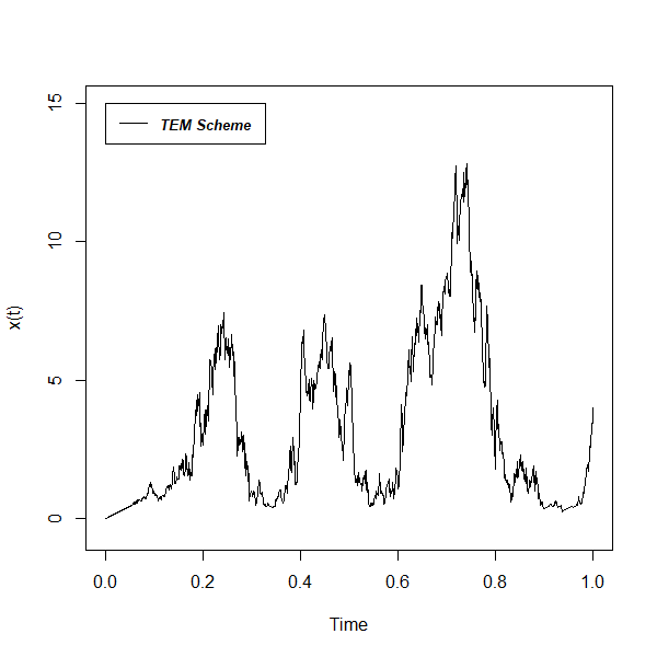
Figure 1: Simulated sample path of $x(t)$ using $\Delta=0.001$

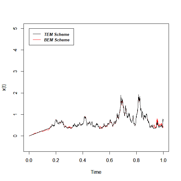
Figure 2: Convergence of TEM and BEM solutions using $\Delta=0.001$

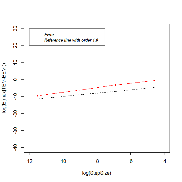
Figure 3: Strong errors between TEM and BEM schemes

7 Applications in finance

In this section, we justify Theorem 5.5 for Monte Carlo valuation of a bond and a barrier option.

7.1 A bond

Suppose the short-term interest rate is governed by SDDE (1). Then a bond price $B$ at maturity time $T$ is given by

$$B(T)=\mathbb{E}\Big{[}\exp\Big{(}-\int_{0}^{T}x(t)dt\Big{)}\Big{]}.$$ (62)

The approximate value of (62) using the step function (25) is computed by

$$B_{\Delta}(T)=\mathbb{E}\Big{[}\exp\Big{(}-\int_{0}^{T}\bar{x}_{\Delta}(t)dt\Big{)}\Big{]}.$$

By Theorem 5.5, we get

$$\lim_{\Delta\rightarrow 0}|B_{\Delta}(T)-B(T)|=0.$$

7.2 A barrier option

Consider the payoff of a path-dependent barrier option at an expiry date $T$ defined by

$$P(T)=\mathbb{E}\Big{[}(x(T)-\Lambda)^{+}1_{\sup_{0\leq t\leq T}}x(t)<\mathbf{B})\Big{]}.$$ (63)

where the barrier, $\mathbf{B}$, and exercise price, $\Lambda$, are constants. Then the approximate value of (63) using (25) is computed by

$$P_{\Delta}(T)=\mathbb{E}\Big{[}(\bar{x}_{\Delta}(T)-\Lambda)^{+}1_{\sup_{0\leq t\leq T}}\bar{x}_{\Delta}(t)<\mathbf{B})\Big{]}.$$

So by Theorem 5.5, we also get

$$\lim_{\Delta\rightarrow 0}|P_{\Delta}(T)-P(T)|=0.$$

The reader is referred to [25] for detailed coverage.

References

- [1] Black, F. and Scholes, M., 1973. The pricing of options and corporate liabilities. Journal of political economy, 81(3), pp.637-654.
- [2] Mao, X. and Sabanis, S., 2013. Delay geometric Brownian motion in financial option valuation. Stochastics An International Journal of Probability and Stochastic Processes, 85(2), pp.295-320.
- [3] Merton, R.C., 1976. Option pricing when underlying stock returns are discontinuous. Journal of financial economics, 3(1-2), pp.125-144.
- [4] Lin, B.H. and Yeh, S.K., 1999. Jump-Diffusion Interest Rate Process: An Empirical Examination. Journal of Business Finance and Accounting, 26(7-8), pp.967-995.
- [5] Kou, S.G., 2002. A jump-diffusion model for option pricing. Management science, 48(8), pp.1086-1101.
- [6] Elliott, R.J., Chan, L. and Siu, T.K., 2013. Option valuation under a regime-switching constant elasticity of variance process. Applied Mathematics and Computation, 219(9), pp.4434-4443.
- [7] Wu, F., Mao, X. and Chen, K., 2008. Strong convergence of Monte Carlo simulations of the mean-reverting square root process with jump. Applied Mathematics and Computation, 206(1), pp.494-505.
- [8] Wu, F., Mao, X. and Chen, K., 2009. The Cox–Ingersoll–Ross model with delay and strong convergence of its Euler–Maruyama approximate solutions. Applied Numerical Mathematics, 59(10), pp.2641-2658.
- [9] Lee, M.K. and Kim, J.H., 2016. A delayed stochastic volatility correction to the constant elasticity of variance model. Acta Mathematicae Applicatae Sinica, English Series, 32(3), pp.611-622.
- [10] Ait-Sahalia, Y., 1996. Testing continuous-time models of the spot interest rate. The review of financial studies, 9(2), pp.385-426.
- [11] Cheng, S.R., 2009. Highly nonlinear model in finance and convergence of Monte Carlo simulations. Journal of Mathematical Analysis and Applications, 353(2), pp.531-543.
- [12] Szpruch, L., Mao, X., Higham, D.J. and Pan, J., 2011. Numerical simulation of a strongly nonlinear Ait-Sahalia-type interest rate model. BIT Numerical Mathematics, 51(2), pp.405-425.
- [13] Dung, N.T., 2016. Tail probabilities of solutions to a generalized Ait-Sahalia interest rate model. Statistics and Probability Letters, 112, pp.98-104.
- [14] Hamilton, J.D., 1988. Rational-expectations econometric analysis of changes in regime: An investigation of the term structure of interest rates. Journal of Economic Dynamics and Control, 12(2-3), pp.385-423.
- [15] Ratanov, N., 2016. Option pricing under jump-diffusion processes with regime switching. Methodology and Computing in Applied Probability, 18(3), pp.829-845.
- [16] Bollen, N.P., Gray, S.F. and Whaley, R.E., 2000. Regime switching in foreign exchange rates:: Evidence from currency option prices. Journal of Econometrics, 94(1-2), pp.239-276.
- [17] Hutzenthaler, M., Jentzen, A. and Kloeden, P.E., 2012. Strong convergence of an explicit numerical method for SDEs with nonglobally Lipschitz continuous coefficients. The Annals of Applied Probability, 22(4), pp.1611-1641.
- [18] Wang, X. and Gan, S., 2013. The tamed Milstein method for commutative stochastic differential equations with non-globally Lipschitz continuous coefficients. Journal of Difference Equations and Applications, 19(3), pp.466-490.
- [19] Liu, W. and Mao, X., 2013. Strong convergence of the stopped Euler–Maruyama method for nonlinear stochastic differential equations. Applied Mathematics and Computation, 223, pp.389-400.
- [20] Mao, X., 2015. The truncated Euler–Maruyama method for stochastic differential equations. Journal of Computational and Applied Mathematics, 290, pp.370-384.
- [21] Coffie, Emmanuel. and Mao, X., 2021. Truncated EM numerical method for generalised Ait-Sahalia-type interest rate model with delay. Journal of Computational and Applied Mathematics, 383, p.113137.
- [22] Mao, X. and Yuan, C., 2006. Stochastic differential equations with Markovian switching. Imperial college press.
- [23] Mao, X., 2007. Stochastic differential equations and applications. 2nd ed. Chichester: Horwood Publishing Limited.
- [24] Yuan, C. and Mao, X., 2010. Stability of stochastic delay hybrid systems with jumps. European journal of control, 16(6), pp.595-608.
- [25] Higham, D.J. and Mao, X., 2005. Convergence of Monte Carlo simulations involving the mean-reverting square root process. Journal of Computational Finance, 8(3), pp.35-61.
- [26] Bao, J., Böttcher, B., Mao, X. and Yuan, C., 2011. Convergence rate of numerical solutions to SFDEs with jumps. Journal of Computational and Applied Mathematics, 236(2), pp.119-131.
- [27] Deng, S., Fei, W., Liu, W. and Mao, X., 2019. The truncated EM method for stochastic differential equations with Poisson jumps. Journal of Computational and Applied Mathematics, 355, pp.232-257.
- [28] Coffie, E., 2021. Delay stochastic interest rate model with jump and strong convergence in Monte Carlo simulations. arXiv preprint arXiv:2103.07651.
- [29] Benth, F.E., 2003. Option theory with stochastic analysis: an introduction to mathematical finance. Berlin: Springer Science and Business Media.
- [30] Oksendal, B., 2013. Stochastic differential equations: an introduction with applications. Springer Science and Business Media.