Numerical instability in B&D models

Abstract

When computing the expected value till extinction of a Birth and Death process, the usual textbook approach results in an extreme case of numerical ill-conditioning, which prevents us from getting accurate answers beyond the first few low-lying states; in this brief note we present a potential solution. We also present a novel derivation of the related formulas.

MCS: 60J80, 65Q30

1 Probability of extinction

Consider a Birth & Death process with rates of $\lambda_{n}$ (for State $n$ to State $n+1$ transition) and $\mu_{n}$ (State $n$ to State $n-1$). When $\lambda_{0}=\mu_{n}=0$, State $0$ is obviously absorbing and the main task is to establish the probability of the process’ ultimate extinction (denoted $a_{i}$), given it starts in State $i.$ Based on what happens during the next transition, the sequence of these probabilities meets the following infinite set of linear equations

$$a_{i}=\frac{\lambda_{i}}{\lambda_{i}+\mu_{i}}~{}a_{i+1}+\frac{\mu_{i}}{\lambda_{i}+\mu_{i}}~{}a_{i-1}$$ (1)

where $i=1,\,2,\,3,\ldots$ and $a_{0}=1$. The last equation can be rewritten as

$$\frac{\lambda_{i}}{\lambda_{i}+\mu_{i}}(a_{i}-a_{i+1})=\frac{\mu_{i}}{\lambda_{i}+\mu_{i}}(a_{i-1}-a_{i})$$ (2)

or, equivalently, introducing $d_{i}=a_{i-1}-a_{i}$

$$d_{i+1}=\frac{\mu_{i}}{\lambda_{i}}~{}d_{i}$$ (3)

Note that

$$a_{i}=1-\sum_{k=1}^{i}d_{k}$$ (4)

To find the solution (see [3]) requires to make State $N$ also absorbing, solving the corresponding finite set of equations, and finally taking the $N\to\infty$ limit. Solving (3) is trivial and yields

$$d_{i}=d_{1}\prod_{n=1}^{i-1}\frac{\mu_{n}}{\lambda_{n}}$$ (5)

Since we have made State $N$ is absorbing, $a_{N}=0$ (i.e. State $0$ cannot be reached from State $N$); this can be restated in the following manner

$$a_{N}=1-\sum_{k=1}^{N}d_{k}=1-d_{1}\sum_{k=1}^{N}\prod_{n=1}^{k-1}\frac{\mu_{n}}{\lambda_{n}}=0$$ (6)

further implying that

$$d_{1}=\frac{1}{\sum_{k=1}^{N}\prod_{n=1}^{k-1}\frac{\mu_{n}}{\lambda_{n}}}$$ (7)

The solution for the $d_{i}$ sequence is thus

$$d_{i}=\frac{\displaystyle\prod_{n=1}^{i-1}\frac{\mu_{n}}{\lambda_{n}}}{\displaystyle\sum_{k=1}^{N}\displaystyle\prod_{n=1}^{k-1}\frac{\mu_{n}}{\lambda_{n}}}\xrightarrow[N\to\infty]{}\frac{\displaystyle\prod_{n=1}^{i-1}\frac{\mu_{n}}{\lambda_{n}}}{\displaystyle\sum_{k=1}^{\infty}\displaystyle\prod_{n=1}^{k-1}\frac{\mu_{n}}{\lambda_{n}}}$$ (8)

which, together with (4), yields any of the probabilities of ultimate extinction. Note that (8) and (4) imply that $\lim_{i\to\infty}a_{i}=0$ when the infinite sum in the last denominator converges, and $a_{i}=1$ for all $i$ when the sum diverges (extinction is then certain for all initial states). Also note that an empty product, i.e. $\prod_{n=1}^{0}\frac{\mu_{n}}{\lambda_{n}}$, equals to $1$.

An alternate approach (see [1]) is to start with

$$a_{0} =1$$ (9)

$$a_{1} =1-\left(\sum_{k=1}^{\infty}\prod_{n=1}^{k-1}\frac{\mu_{n}}{\lambda_{n}}\right)^{-1}$$ (10)

and then iterate using the following recursive formula

$$a_{i+1}=\left(1+\frac{\mu_{i}}{\lambda_{i}}\right)a_{i}-\frac{\mu_{i}}{\lambda_{i}}a_{i-1}$$ (11)

Both algorithms usually work quite well and yield practically identical results, but our recommendation is to use the former one, namely the direct evaluation of (8) followed by (4).

2 Expected time till extinction

When ultimate extinction is certain, the next issue to investigate is: how long does it take to reach State $0$? To find the distribution of this random variable is too difficult to even attempt; we usually settle for the corresponding expected value (denoted $\omega_{i}$, when starting in State $i$). The solution is found by solving the following analog of (1) which similarly relates three consecutive terms of the corresponding sequence of these expected values except now we have to add the expected time till next transition to the RHS, getting

$$\omega_{i}=\frac{\lambda_{i}}{\lambda_{i}+\mu_{i}}~{}\omega_{i+1}+\frac{\mu_{i}}{\lambda_{i}+\mu_{i}}~{}\omega_{i-1}+\frac{1}{\lambda_{i}+\mu_{i}}$$ (12)

or, equivalently

$$\omega_{i+1}=\left(1+\frac{\mu_{i}}{\lambda_{i}}\right)\omega_{i}-\frac{\mu_{i}}{\lambda_{i}}\omega_{i-1}-\frac{1}{\lambda_{i}}$$ (13)

To solve (13), one introduces $\delta_{i}=\omega_{i+1}-\omega_{i}$ which simplifies the previous equation to

$$\delta_{i}=\frac{\mu_{i}}{\lambda_{i}}\delta_{i-1}-\frac{1}{\lambda_{i}}$$ (14)

Its formal solution is

$$\delta_{i}=\sum_{n=i+1}^{\infty}\frac{1}{\lambda_{n}}\prod_{j=i+1}^{n}\frac{\lambda_{j}}{\mu_{j}}+c\prod_{j=1}^{i}\frac{\mu_{j}}{\lambda_{j}}$$ (15)

where $c$ is an arbitrary constant.

Proof.

First we show that the first term of RHS of (15) is a particular solution to (14):

$$\sum_{n=i+1}^{\infty}\frac{1}{\lambda_{n}}\prod\limits_{j=i+1}^{n}\frac{\lambda_{j}}{\mu_{j}}-\frac{\mu_{i}}{\lambda_{i}}\sum_{n=i}^{\infty}\frac{1}{\lambda_{n}}\prod\limits_{j=i}^{n}\frac{\lambda_{j}}{\mu_{j}}$$ (16)

$$=\sum_{n=i+1}^{\infty}\frac{1}{\lambda_{n}}\prod\limits_{j=i+1}^{n}\frac{\lambda_{j}}{\mu_{j}}-\sum_{n=i}^{\infty}\frac{1}{\lambda_{n}}\prod\limits_{j=i+1}^{n}\frac{\lambda_{j}}{\mu_{j}}$$ (17)

$$=-\frac{1}{\lambda_{i}}$$ (18)

The second term is clearly a general solution to the homogeneous version of (14). ∎

Note that $\delta_{i}$ can be interpreted as the expected time till reaching State $i$ (for the first time), given the process starts in State $i+1$; this clearly implies that $\delta_{i}$ cannot be a function of any of the $\lambda_{j}$ and $\mu_{j}$ rates when $j$ is less than or equal to $i$, further implying that $c=0$ (note that the first term of (15) is already free of the irrelevant rates). The final answer is thus

$$\delta_{i}=\sum_{n=i+1}^{\infty}\frac{1}{\lambda_{n}}\prod\limits_{j=i+1}^{n}\frac{\lambda_{j}}{\mu_{j}}$$ (19)

with

$$\omega_{i}=\sum_{k=0}^{i-1}\delta_{k}$$ (20)

An alternate approach (used by both [1] and [2]) would be to first evaluate

$$\omega_{1}=\delta_{0}=\sum_{n=1}^{\infty}\frac{1}{\lambda_{n}}\prod\limits_{j=1}^{n}\frac{\lambda_{j}}{\mu_{j}}$$ (21)

and then use (13) recursively to compute as many terms of the $\omega_{i}$ sequence as needed ($\omega_{0}$ is of course equal to $0$). Unlike in the computation of $a_{i}$, this alternate algorithm results in inaccurate, then incorrect and eventually totally nonsensical values of $\omega_{i}$ as $i$ increases; trying to alleviate this by substantially increasing the accuracy of the computation will only defer the problem to somehow higher values of $i$.

Example 1.

Using $\lambda_{n}=1$ and $\mu_{n}=n$ (one of the simplest such models which, furthermore, leads to the following analytic solution: $\omega_{1}=\delta_{0}=e-1$. Using (13), repeatedly, to find $\omega_{2}$, $\omega_{3}$, …yields nonsensical results starting at $\omega_{20}$; increasing the accuracy to 70 decimal digits still leads to a similar breakdown at $\omega_{52}$, as the corresponding Mathematica program in Figure 1 indicates.

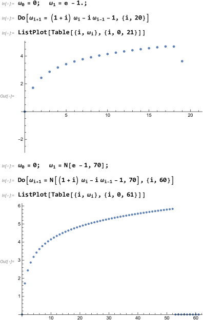
Figure 1: Example 1 results.

Our conclusion (and the main point of this article) is that this algorithm is so badly ill-conditioned that it should never be used.

Instead, we recommend using (19), followed by (20). But even then, similar numerical ill-conditioning may (rather surprisingly) happen when the right hand side of (19) is evaluated analytically (which is possible in some cases). The problem disappears as soon as we switch to numerical evaluation of the same (in Mathematica, this requires using ‘NSum’ instead of ‘Sum’, as the following example demonstrates).

Example 2.

We use the same rates as before, but make the code more general. When we allow Mathematica to convert the RHS of (19) into a formula, its evaluation runs into difficulty at $\omega_{51};$ when we force Mathematica to evaluate the same RHS numerically, correct results are then produced for practically any $\omega_{i}$ (we are demonstrating this up to $\omega_{500}$; in this case we don’t display the corresponding $\delta_{i}$ sequence). See Figure 2.

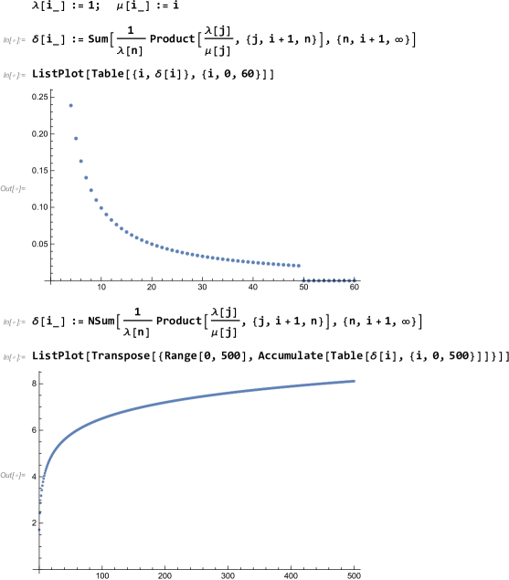
Figure 2: Example 2 results.

Note that no attempt has bee made to optimize our code – the computation is fast enough regardless.

References

[1] Samuel Karlin: “A First Course in Stochastic Processes”,
Academic Press, 1969
[2] Jan Vrbik and Paul Vrbik: “Informal Introduction to Stochastic Processes with Maple”, Springer, 2013
[3] Iosif Pinelis: “Computing probability of ultimate absorption in B&D processes”, Available: https://mathoverflow.net/q/344708 [2021, July]
[4] Iosif Pinelis: “Expected time till extinction in a B&D process”, Available: https://mathoverflow.net/q/345310 [2021, July]