Tensor Methods in Computer Vision and
Deep Learning

Abstract

Tensors, or multidimensional arrays, are data structures that can naturally represent visual data of multiple dimensions. Inherently able to efficiently capture structured, latent semantic spaces and high-order interactions, tensors have a long history of applications in a wide span of computer vision problems. With the advent of the deep learning paradigm shift in computer vision, tensors have become even more fundamental. Indeed, essential ingredients in modern deep learning architectures, such as convolutions and attention mechanisms, can readily be considered as tensor mappings. In effect, tensor methods are increasingly finding significant applications in deep learning, including the design of memory and compute efficient network architectures, improving robustness to random noise and adversarial attacks, and aiding the theoretical understanding of deep networks.

This article provides an in-depth and practical review of tensors and tensor methods in the context of representation learning and deep learning, with a particular focus on visual data analysis and computer vision applications. Concretely, besides fundamental work in tensor-based visual data analysis methods, we focus on recent developments that have brought on a gradual increase of tensor methods, especially in deep learning architectures, and their implications in computer vision applications. To further enable the newcomer to grasp such concepts quickly, we provide companion Python notebooks, covering key aspects of the paper and implementing them, step-by-step with TensorLy.

I Introduction

Tensors are a multidimensional generalization of matrices, and a core mathematical object in multilinear algebra, just like vectors and matrices are in linear algebra. The order of a tensor is the number of indices needed to address its elements. A matrix is a second-order tensor of two modes, namely rows and columns, requiring two indices to access its elements. In analogy, an $N^{\text{th}}$ order tensor has $N$ number of modes, and $N$ indices index it.

Tensors have found tremendous applications in a wide range of disciplines in science and engineering; from many-body quantum systems [1] to algebraic geometry and theoretical computer science [2], to mention a few. In data science and related fields such as machine learning, signal processing, computer vision, and statistics, tensors have been used to represent and analyze information hidden in multi-dimensional data, such as images and videos, or to capture and exploit higher-order similarities or dependencies among vector-valued variables. Just as pair-wise (i.e., second-order) similarities of vector samples are represented by covariance or correlation matrices, a third- (or higher)-order tensor can represent similarities among three (or more) samples in a set. Such tensors are often referred to as higher-order statistics. In this context, tensor methods mainly focus on extending matrix-based learning models such as component analysis [3], dictionary learning e.g., [4], and regression models e.g., [5], to handle data represented by higher-order tensors or estimating parameters of latent variable models by analyzing higher-order statistics [6]. Such developments were for a long time independent of the rise of deep learning, where the concept of a tensor is central. Concretely, besides representing data and statistics, tensors can be viewed as multilinear mappings (i.e., functions), which are higher-order generalizations of linear mappings represented by matrices. For instance, multichannel convolutional kernels, which are the fundamental building blocks of deep convolutional networks, can be readily described using the language of tensors.

This article provides an overview of tensors and tensor methods in the context of representation learning and deep learning, with a particular focus on visual data analysis and computer vision applications.

Tensor structures in visual data. Visual data is a prominent example of multi-dimensional data where a tensor structure is inherent in two main forms:

• Tensor structure of visual measurements: Visual data consist of physically meaningful modes that describe spatial, color, and temporal aspects of the data. Indeed, visual sensors readily generate tensor data: A grayscale image is represented by a matrix whose elements capture the intensity of light along with the spatial coordinates of the image. Hence, a batch of grayscale images is conveniently represented by a third-order tensor with two spatial modes and one mode indexing different images in the batch. A third-order tensor is also a natural way to represent a color image where color channels (e.g., RGB) are stacked along a third mode. Similarly, in tensor representations of hyperspectral and multispectral images, different channels capturing different spectral bands of light are stacked along with the third mode. Tensors of fourth-order are also being used to represent visual data that includes a time mode, in addition to the spatial and spectral/color modes. Higher-order tensor structure also arises in medical imaging. For instance, magnetic resonance imaging (MRI) and functional magnetic resonance imaging (fMRI), are naturally stored in a multidimensional array such as a matrix (e.g., a two-dimensional (2D) MRI image), a third-order tensor (e.g., a three-dimensional (3D) MRI image), or a fourth-order tensor (e.g., a 3D fMRI image over time).

• Latent tensor structure in image formation: Image formation relies upon the interactions of multiple latent factors of variation related to appearance (e.g., illumination, pose) or even image semantics (such as gender and age in human faces). Such factors are often entangled through a multilinear (tensor) mapping in an unobserved, latent space that gives rise to the rich visual data structure. This tensor mapping assumes that visual variation is linear if we keep all but one factor constant. For example, in facial images, changing the illumination does not change the depicted person’s identity.

Typical computer vision and visual data analysis applications, such as detecting objects and recognizing faces in images and videos, understanding human behavior in videos (e.g., action and activity recognition), enhancing the quality of images (i.e., image denoising and inpainting), and generating novel visual content (i.e., image synthesis), require the extraction of physically–or semantically–meaningful representations of visual data. Traditional machine learning models employed towards this end, such as component analysis, sparse coding, and regression functions, treat data points as vectors and datasets as matrices. Hence, multi-dimensional visual data samples need to be flattened into very high-dimensional vectors, where natural topological structures and dependencies among different modes (e.g., spatial and temporal) of measurements are lost. Besides structure loss, when high-dimensional vectors are employed in training matrix-based machine learning models, the number of data samples needed to estimate an arbitrary function (or parameters of a machine learning model) within a given level of accuracy grows exponentially with data dimensionality. This phenomenon is known as the curse of dimensionality [7].

Tensor methods in representation learning for computer vision: Tensor methods have emerged as a powerful tool for learning representations from multidimensional data by mitigating the curse of dimensionality without discarding their structure, which carries useful information in the case of visual data. Indeed, being able to both recover latent factors in visual data and flexible enough to accommodate a large set of structural constraints and regularizations, tensor decomposition and tensor component analysis methods have had a transformative impact in a wide range of computer vision applications, ranging from human sensing (face and body analysis) to medical and hyperspectral imaging. In this context, dimensionality reduction, clustering, and data compression rely on decompositions of tensors representing visual data [8]. Non-negative factorization of such data tensors results in representations that correspond to local parts of the visual object [9]. Decomposing visual data into shape and motion factors, or surface normal and reflectance factors, facilitates the recovery of structure from motion and provides solutions to photometric stereo, e.g., [10]. Tensor decompositions with sparse regularization [11, 4] have proven to be very useful in inverse problems in imaging, such as denoising and inpainting.

Recently, deep learning models have led to qualitative breakthroughs on a wide variety of computer vision applications, among many other machine learning tasks [12]. Deep neural networks act as learnable approximations of high-dimensional, non-linear functions. For example, in image classification, one seeks to learn an unknown high-dimensional target function that maps an input image to the output label. The key ingredient of their success is that deep learning models leverage statistical properties of data such as stationarity (e.g., shift-invariance) and compositionality (e.g., the hierarchical structure of images) through local statistics, which are present in visual data [13, 14, 15]. These properties are exploited by convolutional architectures [13, 16], which are built of alternating multidimensional convolutional layers, point-wise nonlinear functions (e.g., ReLU), downsampling (pooling) layers, while also containing tensor-structured fully-connected layers. The use of multidimensional convolutions in deep neural networks allows extracting local features shared across the image domain. In turn, this greatly reduces the number of learnable parameters and consequently alleviates the effect of the curse of dimensionality–without sacrificing the ability to approximate the target function.

Tensor methods in deep learning architectures for computer vision: Despite the compositional structure of deep neural networks that mitigates the curse of dimensionality, deep learning models are usually over-parameterized involving an enormous number (typically tens of millions or even billions) of unknown parameters. Even though over-parametrization of deep neural networks allows finding good local minima, particularly when they are trained with gradient descent [17, 18], such a large number of trainable parameters makes deep networks prone to overfitting and noise  [19], hindering the analysis of their generalization properties (i.e., how well they perform on unseen data) [20]. Tensor decompositions can significantly reduce the number of unknown parameters of deep models and further mitigate the curse of dimensionality. Indeed, tensor decompositions can be applied to the weights of neural network layers to compress them, and in some cases, speed them up [21, 22, 23]. In addition, using tensor-based operations within deep neural networks allows to preserve and leverage the topological structure in the data while resulting in parsimonious models [24, 25]. In convolutional neural networks (CNNs), (non-separable) multichannel convolution kernels can be decomposed into a sum of mode-separable convolutions using low-rank tensor decompositions, resulting in network compression and a reduction in the number of parameters [26, 27]. Deep network compression is significant in the deployment of deep learning models in resource-limited devices, while reducing the number of parameters acts as implicit regularization that improves generalization across tasks and domains [28, 29, 30]. Furthermore, randomized tensor decomposition of neural networks’ building blocks has been proved effective in robustifying neural networks against adversarial attacks [31, 32] and to various types of random noise–such as noise occurring naturally when capturing data such as MRI [33].

Surveys that approach tensors from varying perspectives have emerged over the past years. In [34], one of the most prominent and influential overviews of tensor decompositions is presented, while in [35], a mathematical account for multilinear mappings is provided. While [34, 35] target audiences mostly from an applied mathematics perspective, other surveys focus on applications of tensors in scientific and engineering fields; indicatively, in areas such as signal processing and machine learning [36, 37], data mining and fusion [38], multidimensional data analysis [39, 40], blind source separation [41], computer vision [3, 8], and spectral learning [6, 42].

While the surveys mentioned above cover an impressive spectrum of theoretical and algorithmic developments and applications, one can identify a gap in the literature concerning recent advancements in the use of tensor methods in the context of representation learning and deep learning for computer vision. In this paper, besides fundamental work in tensor learning for computer vision, we focus on recent developments that have brought on a gradual increase of tensor-related methods, especially in deep learning architectures, and their implications in vision applications. To further enable the newcomer to grasp such concepts quickly, we provide thorough tutorial-style companion notebooks in Python, covering every section of the paper.

Structure of the paper. The remainder of the paper is organized as follows. In Section II, tensor and matrix algebra fundamentals are presented. In Section III, an overview of existing computational tools and the necessary infrastructure is discussed, focusing on the TensorLy library on which the companion notebooks of this paper are based. Section IV provides an introduction to representation learning with tensors. In Section V, recent research that utilizes tensor methods in deep learning architectures are detailed, while related applications in computer vision are discussed in Section VI. Finally, a summary of practical challenges is presented in Section VII, along with advice to practitioners.

II Preliminaries on Matrices and Tensors

Notebook: tensor_manipulation.ipynb

Multilinear algebra is much richer than its linear counterpart and hence tensor algebra notation and manipulation of tensors may appear complicated to newcomers in the field. To make the paper self-contained and give the reader an understanding of the mathematical tools employed in tensor methods for learning, we first introduce the notation conventions used in this paper and then review some of the fundamental concepts of linear and mutlilinear algebra.

To ensure consistency in terminology that would be familiar to machine learning and computer vision researchers we have adopted the terminology employed in relevant overview papers [36, 34, 6] and recent publications on these topics. The notation used here is very similar to that adopted in [36, 34, 43]. However, we differentiate on one point: we employ a different ordering of elements when tensors are flattened to matrices than that used in [34] and may be familiar to some of the readers (cf. Definition II.1).

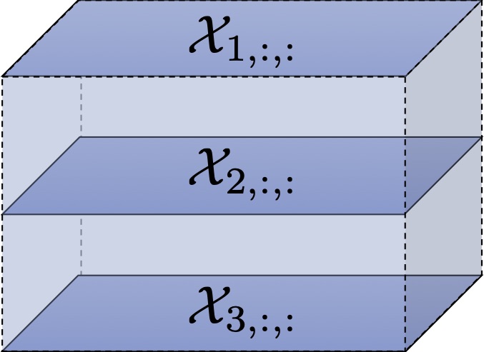
(a) Horizontal Slices

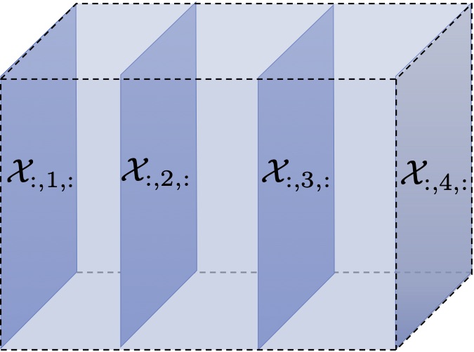
(b) Lateral Slices

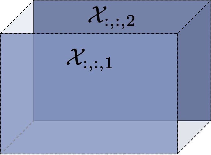
(c) Frontal Slices

Figure 1: Illustration of the slices of a third order tensor of size $3\times 4\times 2$

II-A Notation

Scalars are denoted by plain letters i.e., $x,I,J$. First order tensors are vectors, denoted as $\mathbf{x}$. Second order tensors are matrices, denoted as $\mathbf{X}$. $\mathbf{I}$ denotes the identity matrix of compatible dimensions. The transpose of $\mathbf{X}$ is denoted $\mathbf{X}^{\top}$. The $i$th column of $\mathbf{X}$ is denoted as $\mathbf{x}_{i}$.

The sets of real and integer numbers are denoted by $\mathbb{R}$ and $\mathbb{Z}$, respectively. A set of $M$ real matrices (vectors) of varying dimensions is denoted by $\{\mathbf{X}^{(m)}\in\mathbb{R}^{I_{m}\times N}\}_{m=1}^{M}$ $(\{\mathbf{x}^{(m)}\in\mathbb{R}^{I_{m}}\}_{m=1}^{M})$. Finally, for any $i,j\in\mathbb{Z}$, with $i<j$, $[{i}\mathrel{{.}\,{.}}\nobreak{j}]$ denotes the set of integers $\{i,i+1,\cdots,j-1,j\}$.

Tensors of order three or higher are denoted by $\mathcal{{X}}$. The reader is reminded that the order of a tensor is the number of indices (dimensions) needed to address its elements. Each dimension is called a mode. Specifically, an $N^{\text{th}}$ order tensor has $N$ indices, with each index addressing a mode of $\mathcal{{X}}$. Assuming $\mathcal{{X}}$ is real-valued, it is defined over the tensor space $\mathbb{R}^{I_{1}\times I_{2}\times\cdots\times I_{N}}$, where $I_{n}\in\mathbb{Z}$ for $n=1,2,\ldots,N$. An element $(i_{1},i_{2},\cdots,i_{N})$ of tensor $\mathcal{{X}}\in\mathbb{R}^{I_{1}\times I_{2}\times\cdots\times I_{N}}$ is accessed as: $\mathcal{{X}}_{i_{1},i_{2},\cdots,i_{N}}$ or $\mathcal{{X}}(i_{1},i_{2},\cdots,i_{N})$. This corresponds to viewing a tensor as a multi-dimensional array in $\mathbb{R}^{I_{1}\times I_{2}\times\cdots\times I_{N}}$. Furthermore, given a set of $N$ vectors (or matrices) that correspond to each mode of $\mathcal{{X}}$, the $n^{\text{th}}$ vector (or matrix) is denoted as $\mathbf{u}^{(n)}$ (or $\mathbf{U}^{(n)}$).

Fibers are a generalization of the concept of rows and columns of matrices to tensors. They are obtained by fixing all indices but one. A colon is used to denote all elements of a mode e.g., the mode-1 fibers of $\mathcal{{X}}$ are denoted as $\mathcal{{X}}_{:,i_{2},i_{3}}$.

Slices (Figure 1) are obtained, for a third-order tensor, by fixing one of the indices.

Fibers	mode-0 fibers	mode-1 fibers	mode-2 fibers
2-4 TensorLy	mode-0 unfolding	mode-1 unfolding	mode-2 unfolding
2-4 Matlab	mode-0 unfolding	mode-1 unfolding	mode-2 unfolding

TABLE I: Illustration of the fibers and unfolding of a third order tensor.

II-B Transforming tensors into matrices and vectors

Definition II.1 (Tensor unfolding):

Given a tensor, $\mathcal{{X}}\in\mathbb{R}^{I_{1}\times I_{2}\times\cdots\times I_{N}}$, its mode-$n$ unfolding is a matrix $\mathbf{X}_{[n]}\in\mathbb{R}^{I_{n}\times I_{M}}$, with $M=\prod_{\begin{subarray}{c}k=1,\\ k\neq n\end{subarray}}^{N}I_{k}$ and is defined by the mapping from element $(i_{1},i_{2},\cdots,i_{N})$ to $(i_{n},j)$, with $j=1+\sum_{\begin{subarray}{c}k=1,\\ k\neq n\end{subarray}}^{N}(i_{k}-1)\times\prod_{\begin{subarray}{c}m=k+1,\\ m\neq n\end{subarray}}^{N}I_{m}$.

Tensor unfolding corresponds to a reordering of the fibers of the tensor as the columns of a matrix. There are more than one definition of tensor unfolding, which vary by the ordering of the fibers. In particular, our definition corresponds to a row-wise underlying ordering (or C-ordering ) of the elements. The main other definition, popularised by Kolda and Bader [34], corresponds to a column-wise (or Fortran) ordering of the elements, which is more efficient for libraries using that ordering, such as MATLAB. Conversely, our definition naturally leads to better performance for implementation with C-ordering of the elements, which is the case with most Python/C++ software libraries as well as most GPU libraries [44]. Table I illustrates the link between the fibers and the unfoldings, as well as the difference between our definition (row-wise, or C-ordering) and the column-wise, or Fortran ordering [34].

Definition II.2 (Tensor vectorization):

Given a tensor, $\mathcal{{X}}\in\mathbb{R}^{I_{1}\times I_{2}\times\cdots\times I_{N}}$, we can flatten it into a vector $\text{vec}(\mathcal{{X}})$ of size $I_{1}\cdot I_{2}\cdot\ldots\cdot I_{N}$ defined by the mapping from element $(i_{1},i_{2},\cdots,i_{N})$ of $\mathcal{{X}}$ to element $j$ of $\text{vec}(\mathcal{{X}})$, with $j=1+\sum_{k=1}^{N}(i_{k}-1)\times\prod_{m=k+1}^{N}I_{m}$.

II-C Matrix and tensor products

Here, we will define several matrix and tensor products employed by the surveyed methods.

Definition II.3 (Kronecker product):

Given two matrices $\mathbf{A}\in\mathbb{R}^{I_{1}\times I_{2}}$ and $\mathbf{B}\in\mathbb{R}^{J_{1}\times J_{2}}$, their Kronecker product is defined as:

$$\mathbf{A}\otimes\mathbf{B}=\begin{bmatrix}a_{11}\mathbf{B}&\cdots&a_{1I_{2}}\mathbf{B}\\ \vdots&\ddots&\vdots\\ a_{I_{1}1}\mathbf{B}&\cdots&a_{I_{1}I_{2}}\mathbf{B}\end{bmatrix}\in\mathbb{R}^{I_{1}\cdot J_{1}\times I_{2}\cdot J_{2}}$$

Definition II.4 (Khatri-Rao product):

Given two matrices $\mathbf{A}\in\mathbb{R}^{I\times R}$ and $\mathbf{B}\in\mathbb{R}^{J\times R}$ with the same number of columns, their Khatri-Rao product, also known as column-wise Kronecker product, is defined as $\mathbf{A}\odot\mathbf{B}\in\mathbb{R}^{I\cdot J\times R}$:

$$\mathbf{A}\odot\mathbf{B}=\left[\begin{matrix}\mathbf{A}_{:,1}\otimes\mathbf{B}_{:,1},&\mathbf{A}_{:,2}\otimes\mathbf{B}_{:,2},&\cdots,&\mathbf{A}_{:,R}\otimes\mathbf{B}_{:,R}\end{matrix}\right]$$

Furthermore, the Khatri-Rao product of a set of $M$ matrices $\{\mathbf{X}^{(m)}\in\mathbb{R}^{I_{m}\times N}\}_{m=1}^{M}$ is denoted by $\mathbf{X}^{(1)}\odot\mathbf{X}^{(2)}\odot\cdots\odot\mathbf{X}^{(M)}$.

Definition II.5 (Hadamard product):

The Hadamard product of $\mathbf{A},\mathbf{B}\in\mathbb{R}^{I\times J}$ is the element-wise product is symbolized as $\mathbf{A}*\mathbf{B}$ and is defined element-wise as $\mathbf{A}_{(i,j)}\mathbf{B}_{(i,j)}$.

Definition II.6 (Outer product):

$\circ$ denotes the vector outer product. Given a set of $N$ vectors $\{\mathbf{x}^{(n)}\in\mathbb{R}^{I_{n}}\}_{n=1}^{N}$ their outer product is denoted as $\mathcal{{X}}=\mathbf{x}^{(1)}\circ\mathbf{x}^{(2)}\circ\cdots\circ\mathbf{x}^{(N)}\in\mathbb{R}^{I_{1}\times I_{2}\times\cdots\times I_{N}}$ and defines a rank-one $N^{\text{th}}$-order tensor.

Definition II.7 ($n$-mode product):

For a tensor $\mathcal{{X}}\in\mathbb{R}^{I_{1}\times I_{2}\times\cdots\times I_{N}}$ and a matrix $\mathbf{M}\in\mathbb{R}^{R\times I_{n}}$, the n-mode product of a tensor is a tensor of size $\left(I_{1}\times\cdots\times I_{n-1}\times R\times I_{n+1}\times\cdots\times I_{N}\right)$ and can be expressed using unfolding of $\mathcal{{X}}$ and the classical dot product as:

$$\mathcal{{X}}\times_{n}\mathbf{M}=\mathbf{M}\mathbf{X}_{[n]}\in\mathbb{R}^{I_{1}\times\cdots\times I_{n-1}\times R\times I_{n+1}\times\cdots\times I_{N}}$$

The $n$- mode vector product of a tensor $\mathcal{{X}}\in\mathbb{R}^{I_{1}\times I_{2}\times\ldots\times I_{N}}$ with a vector $\mathbf{x}\in\mathbb{R}^{I_{n}}$ is denoted by $\mathcal{{X}}\times_{n}\mathbf{x}\in\mathbb{R}^{I_{1}\times I_{2}\times\cdots\times I_{n-1}\times I_{n+1}\times\cdots\times I_{N}}$. The resulting tensor is of order $N-1$ and is defined element-wise as

$$(\mathcal{{X}}\times_{n}\mathbf{x})_{i_{1},\ldots,i_{n-1},i_{n+1},\ldots,i_{N}}=\sum_{i_{n}=1}^{I_{n}}x_{i_{1},i_{2},\ldots,i_{N}}x_{i_{n}}.$$ (1)

In order to simplify the notation, we denote $\bm{\mathcal{X}}\times_{1}\mathbf{x}^{(1)}\times_{2}\mathbf{x}^{(2)}\times_{3}\cdots\times_{N}\mathbf{x}^{(N)}=\bm{\mathcal{X}}\prod_{n=1}^{N}\times_{n}\mathbf{x}^{(n)}$.

Definition II.8 (Generalized inner-product):

For two tensors $\mathcal{{X}},\mathcal{{Y}}\in\mathbb{R}^{I_{1}\times I_{2}\times\cdots\times I_{N}}$ of same size, their inner product is defined as $\langle{\mathcal{{X}}},{\mathcal{{Y}}}\rangle=~{}\sum_{i_{1}=1}^{I_{1}}\sum_{i_{2}=1}^{I_{2}}\cdots\sum_{i_{n}=1}^{I_{N}}\mathcal{{X}}_{i_{1},i_{2},\cdots,i_{n}}\mathcal{{Y}}_{i_{1},i_{2},\cdots,i_{n}}$ For two tensors $\mathcal{{X}}\in\mathbb{R}^{D_{x}\times I_{1}\times I_{2}\times\cdots\times I_{N}}$ and $\mathcal{{Y}}\in\mathbb{R}^{I_{1}\times I_{2}\times\cdots\times I_{N}\times D_{y}}$ sharing $N$ modes of same size, we similarly define the generalized inner product along the $N$ last (respectively first) modes of $\mathcal{{X}}$ (respectively $\mathcal{{Y}}$) as

$$\langle{\mathcal{{X}}},{\mathcal{{Y}}}\rangle_{N}=~{}\sum_{i_{1}=1}^{I_{1}}\sum_{i_{2}=1}^{I_{1}}\cdots\sum_{i_{n}=1}^{I_{N}}\mathcal{{X}}_{:,i_{2},i_{3},\cdots,i_{n}}\mathcal{{Y}}_{i_{1},i_{2},\cdots,i_{n-1},:}$$

with $\langle{\mathcal{{X}}},{\mathcal{{Y}}}\rangle_{N}\in\mathbb{R}^{I_{x}\times I_{y}}$.

Definition II.9 (Convolution):

We denote a regular convolution of $\mathcal{{X}}$ with $\mathbf{W}$ as $\mathcal{{X}}\star\mathbf{W}$. For $1$–D convolutions, we write the convolution of a tensor $\mathcal{{X}}\in\mathbb{R}^{I_{1}\times I_{2}\times\cdots\times I_{N}}$ with a vector $\mathbf{v}\in\mathbb{R}^{K}$ along the $n^{\text{th}}$–mode as $\mathcal{{X}}\star_{n}\mathbf{v}$. In practice, as done in current deep learning frameworks [45], we use cross-correlation, which differs from a convolution by a flip of the kernel. This does not impact the results since the weights are learned end-to-end. In other words, $\left(\mathcal{{X}}\star_{n}\mathbf{v}\right)_{i_{1},\cdots,i_{N}}=\sum_{k=1}^{K}\mathbf{v}_{k}\mathcal{{X}}_{i_{1},\cdots,i_{n-1},i_{n}+k,i_{n+1},\cdots,I_{N}}$.

II-D Tensor diagrams

Most tensor methods involve a series of tensor operators, such as tensor contractions, resulting in several sums over various modes and tensors, with as many indices, which can be cumbersome to read and write.

Tensor diagrams are pictorial representations of tensor algebraic operations, in the form of undirected graphs offering a more intuitive way to read and write tensor operators and design tensor methods. The vertices (circles) represent tensors, and its edge the modes of that tensor. The degree of each vertex (the number of edges coming out of it) thus represents the order of the corresponding tensor. Consequently, using tensor diagrams a scalar (Fig. 2(a)) would simply be represented by a vertex while a vector (i.e., a tensor with one index) would have one edge. A matrix (Fig. 2(b)) would be a vertex with two edges, and so on for third- (Fig. 2(c)) and fourth-order (Fig. 2(d)) tensors.

(a) vector

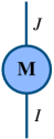
(b) matrix

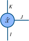
(c) $3^{\text{rd}}$ order tensor

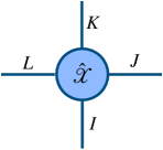
(d) $4^{\text{th}}$ order tensor

Figure 2: Representation of tensors of various orders using tensor diagrams. The vertices represent tensors and their degree the order of the tensors.

By employing tensor diagrams, tensor contraction over a common dimension of two tensors is represented by connecting the two corresponding edges. For instance, given matrices $\mathbf{A}\in\mathbb{R}^{I\times J},\mathbf{B}\in\mathbb{R}^{J\times K}$, we can express simply their product $\mathbf{C}=\mathbf{A}\mathbf{B}=\sum_{j=1}^{J}\mathbf{a}_{:,j}\mathbf{b}_{j,:}^{{}^{\top}}$, as illustrated in Fig. 3(a).

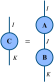
(a) matrix product

(b) inner-product (vectors)

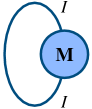
(c) matrix trace

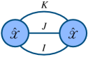
(d) inner-product (tensors)

Figure 3: Representation of some tensor contractions using tensor diagrams

II-E Matrix rank

The rank of a matrix can be defined in several equivalent ways. Hereby we give a simple definition:

Definition II.10 (Matrix rank):

Let $\mathbf{X}\in\mathbb{R}^{I\times J}$ an $I\times J$ matrix of real numbers. The rank of $\mathbf{X}$ is denoted as rank$(\mathbf{X})$. It is equivalently defined as:

• The number of linearly independent columns of $\mathbf{X}$

• The number of linearly independent rows of $\mathbf{X}$

The above definition immediately implies that if $\mathbf{X}\in\mathbb{R}^{I\times J}$, then rank$(\mathbf{X})\leq\min(I,J)$. If rank$(\mathbf{X})=\min(I,J)$ then $\mathbf{X}$ is full-rank.

II-F Norms

One of the major families of tensor norms, of any order, is element-wise norms.

Definition II.11 ($\ell_{p}$ norm):

The element-wise $\ell_{p}$ of $\mathcal{{X}}$ is:

$$\|\mathcal{{X}}\|_{p}=\|\text{vec}(\mathcal{{X}})\|_{p}=\left(\sum_{i_{1},i_{2},\cdots,i_{N}}|\mathcal{{X}}_{i_{1},i_{2},\cdots,i_{N}}|^{p}\right)^{1/p}$$

For $p=0$, the $\ell_{0}$ (pseudo)-norm, denoted $\|\mathcal{{X}}\|_{0}$ returns the number of non-zero elements of a tensor, acting as a measure of the density (and conversely of the sparsity) of the tensor. However, it is not exactly a norm in the mathematical sense (it is positive definite and satisfies the triangle inequality but is not absolutely homogeneous), hence the name pseudo-norm. When $p=1$ the $\ell_{1}$-norm is denoted by $\|\mathcal{{X}}\|_{1}$ and is defined as the sum of the absolute values of the tensor’s elements. The $\ell_{1}$-norm is the tightest convex surrogate of $\ell_{0}$-norm [46] and is used as a convenient measure of sparsity in practice. For $p=2$, the Frobenius norm is denoted as $\|\mathbf{X}\|_{F}$ for matrices and it is generalized to higher-order tensors by the tensor norm, denoted $\|\mathcal{{X}}\|$.

The family of Schatten-$p$ norms are defined for matrices and act as functions of the singular values (i.e., spectrum) of the matrix. Therefore, Schatten-$p$ norms can be used to control the spectral properties of matrices.

Definition II.12 (Schatten-$p$ norm):

Let $[\sigma_{1},\sigma_{2},\ldots,\sigma_{\min(I,J)}]^{\top}$ be a vector of the singular values of $\mathbf{X}\in\mathbb{R}^{I\times J}$. A Schatten-$p$ norm is obtained by taking the $p$ norm of the singular values:

$$\|\mathbf{X}\|_{p}=\left(\sum_{i}^{\min(I,J)}\sigma_{i}^{p}\right)^{1/p}$$

For $p=1$, the Schatten-$1$ norm is referred to as the nuclear norm and denoted by $\|\mathbf{X}\|_{*}$. It is defined as the sum of the singular values of $\mathbf{X}$ and is the tightest convex envelope of the rank function [47].

III Computational Infrastructure and Tools

In this section, we discuss the necessary infrastructure for computer vision and deep learning. Also, to accelerate the learning curve and enable researchers and practitioners to get started in the field of tensor methods quickly, we review available software packages for tensor algebra and introduce the TensorLy library [44], with which we implement ready-to-use examples that accompany the paper.

III-A Hardware

Enabling deep learning, computer vision, and machine learning start in general down at the hardware level. Indeed, modern computer vision is enabled by the “trinity of AI”: data, with the introduction of large bodies of annotated data; algorithms, with the introduction of convolutional neural networks, recurrent units, etc. and finally hardware, with the use of graphical processing units (GPUs). The latter was crucial in scaling up computation and enabling training on big (visual) data consisting of millions of images.

Historically, datasets used in computer vision were relatively small and could easily fit in the memory of most commodity personal computers. However, with the advent of deep learning and large bodies of annotated images, such as ImageNet [14], it became crucial to have large amounts of memory. Most importantly, to be able to process the information efficiently, it became paramount to be able to process multiple bits of information in parallel. However, central processing units (CPUs) are inherently sequential. First proposed in [48], then successfully used on MNIST [49] and more prominently, on ImageNet [14], it is the use of GPUs that revolutionized deep learning, making it feasible to train a very large model on millions of samples. While CPUs perform operations on tensors in a mostly sequential way and prioritize low latency, GPUs favor high throughput and accelerate operations by running them efficiently in parallel: modern CPUs typically contain up to $16$ cores, while a GPU has thousands of them, allowing for the performance of hundreds of TFLOPS.

Efficient libraries then enable to efficient use of the tensor cores composing GPUs. In particular, extending Basic Linear Algebra Subprograms (BLAS) primitives allows to significantly speed up computation by leveraging hardware acceleration [50]. The recent cuTensor [51] is a high-performance CUDA library that leverages GPU-acceleration for efficient tensor operations. In particular, it obviates the need for costly reordering of the elements and reshaping when performing operations such as tensor contraction for which it provides native implementations.

Further, large models typically need to be trained on multiple GPUs distributed in various machines. However, distributed training and inference across multiple machines introduces new challenges and can be incredibly complex to implement correctly. Fortunately, modern deep learning libraries abstract such technicalities and allow the end-user to focus on the model’s logic. Notable such frameworks include PyTorch [45], which offers a functional approach to deep learning, and TensorFlow [52], which uses a symbolic one. Others such as MXNet [53] enable a hybrid approach.

While CPU and GPU are the most widely used mediums for training and inference in computer vision and deep learning tasks, other hardware types can be used towards this end. Examples include application-specific integrated circuits (ASICs) designed specifically for running a specialized set of instructions (e.g., TPUs [54]), or field-programmable gate arrays (FPGAs) that conversely can be dynamically programmed depending on the application.

III-B Software

In the previous section, we covered hardware support, however, there is a considerable interplay between hardware and software, and one cannot function well without the other. Good software without optimized hardware support would result in slow training, while sub-par software with poor API, documentation, and tests is unusable in practice. An example of this interplay is the organization of elements in memory. Memory can be over-simplified as one long vector of numbers. The way these elements are ordered in memory influences how fast operations are executed. For instance, to store a matrix, its elements can be arranged row-after-row (C-ordering) or column-after-column (also called Fortran ordering). In NumPy, elements are organized by default in row-order–the same for PyTorch. This, in turn, influences higher-level operations: unfolding, for instance, needs to be adapted to appropriate ordering to avoid expensive reordering of the data. As a result, much effort has been spent developing user-friendly libraries that provide state-of-the-art algorithms, neatly coded and wrapped in an intuitive, well-tested API. One notable such library is TensorLy [44].

Figure 4: Overview of the TensorLy and TensorLy-Torch libraries

TensorLy is a Python library that aims at making tensor learning simple and accessible. It provides a high-level API for tensor methods, including core tensor operations, tensor decomposition, regression, and deep tensorized architectures. It has a flexible backend that allows running operations seamlessly using NumPy, PyTorch, TensorFlow, etc. The project is also open-sourced under the BSD license, making it suitable for both academic and commercial use. TensorLy is also optimized for Python and its ecosystem. For instance, the unfolding is redefined as introduced in Section II to match the underlying C-ordering of the elements in memory, resulting in better performance. An overview of the functionalities of TensorLy can be seen in Figure 4. By default, it uses NumPy as its backend. However, this can be set to any of the deep learning frameworks, optimized for running large-scale methods, and in the companion, we also use the popular PyTorch library. Once PyTorch has been installed, it can be easily used as a backend for TensorLy, allowing all the operations to run transparently on multiple machines and GPU. Finally, TensorLy-Torch [55] builds on top of TensorLy and PyTorch and implements out-of-the-box layers for tensor operations within deep neural networks.

Other libraries exist for tensor operations in Python. In particular, t3f [56] is a TensorFlow library for working with the tensor-train decomposition on CPU and GPU. It also supports Riemannian optimization operations. Tntorch [57] is a library for tensor networks in PyTorch, while TensorNetwork [58] additionally supports JAX, TensorFlow and NumPy. Scikit-Tensor [59] is a NumPy library for tensor learning, supporting several tensor decompositions.

In MATLAB, packages such as the Tensor Toolbox [60] or TensorLab [61] provide extensive support for tensor decomposition. In C++, ITensor [62] provides efficient support for tensor network calculations.

Finally, efficient operations on sparse tensors require specialized implementations. Indeed, while libraries such as NumPy are highly-optimized for matrix and tensor contractions, they do not support operations on sparse tensors. Explicitly representing sparse tensors as dense arrays is very inefficient in terms of memory use and prohibitive for very large tensors. Instead, these can be represented efficiently, e.g., using the COOrdinate format which instead of storing all the elements only stores the coordinates and values of non-zero elements. As a result, implementing them efficiently can be tricky. While there is a large body of work focusing on sparse matrix support, support for sparse tensor algebra is more scant. Libraries such as the PyData Sparse for CPU and the Minkowski Engine [63] for GPU are being developed and provide an efficient way to leverage large, sparse multi-dimensional data. TensorLy also supports sparse tensor operations on CPU through the PyData Sparse library.

IV Representation Learning with Tensor Decompositions

IV-A Matrix decomposition and representation learning

Real-world visual data exhibit complex variability due to many factors related to visual objects’ appearance (e.g., illumination and pose changes, rigid and non-rigid deformations), image structure, semantics, and noise. Hence, useful information is hidden in high-dimensional visual measurements. Representation learning methods seek to extract useful information from such high-dimensional data through simple, low-dimensional representations (i.e., data are expressed as a linear combination of basic yet fundamental structures) that simultaneously exhibit a set of desirable properties such as invariance to nuisance variability while at the same time recovering factors of variation in a meaningful manner for a specific task. In practice, low-rank and sparsity are popular simplicity measures used in representation learning models.

Matrix decomposition forms the mathematical backbone in learning parsimonious, low-dimensional representations from high-dimensional vector data samples, such as images flattened into vectors. Component analysis, e.g., [64] and sparse coding, e.g., [65, 66] are prominent examples of representation learning methods that extract simple data representations by means of low-rank matrix decompositions and sparse, possibly overcomplete representations, respectively. Given $M$ vector data samples $\{\mathbf{x}_{m}\}_{m=1}^{M}$, where each sample $\mathbf{x}_{m}$ is an $I$-dimensional vector, that is $\mathbf{x}_{m}\in\mathbb{R}^{I}_{m}$, such a dataset can be represented by a data matrix $\mathbf{X}\in\mathbb{R}^{I\times J}$ which contains in its columns data vectors. Matrix decompositions seek to factorize $\mathbf{X}$ as a product of two factor matrices $\mathbf{U}^{(1)}\in\mathbb{R}^{I\times R}$ and $\mathbf{U}^{(2)}\in\mathbb{R}^{J\times R}$, namely

$$\mathbf{X}=\mathbf{U}^{(1)}{\mathbf{U}^{(2)}}^{\top}.$$ (2)

Assuming $\mathbf{X}$ is of low-rank $R<\min\{I,J\}$, Eq. (2) is referred to as low-rank matrix decomposition. Hence, $\mathbf{X}$ can be expressed as a sum of $R$ rank-one matrices: $\mathbf{X}=\mathbf{U}^{(1)}{\mathbf{U}^{(2)}}^{\top}=\sum_{r=1}^{R}\mathbf{u}^{(1)}_{r}\circ{\mathbf{u}^{(2)}_{r}}=\sum_{r=1}^{R}\mathbf{u}^{(1)}_{r}{\mathbf{u}^{(2)}_{r}}^{\top}.$ The concept of low-rank matrix decomposition is generalized for higher-order tensors by low-rank tensor decomposition which will be discussed next in Section IV-B. Interestingly, as opposed to matrix decomposition which is not unique low-rank tensor decomposition, such as the Canonical-Polyadic decomposition, also known as Parallel Factor Analysis (PARAFAC) [67, 68, 69] is unique under mild algebraic assumptions (see [36] and references therein).

In practice, data matrices representing visual data sets are not exactly low-rank. The observed matrix can deviate from the low-rank structure for several reasons, including noise, outliers, and non-linear structures underlying the data. In such cases, we are interested in approximating the observed matrix with a low-rank matrix expressed as a product of two factor matrices. Depending on the application, these elements can be interpreted either as a basis of a low-dimensional subspace or as a mixing operator (i.e., mixing matrix) that combines hidden factors of variation, giving rise to the observed data. Such components comprise a low-dimensional, and hence a simplified representation of the data in the subspace spanned by the basis elements. To ensure uniqueness and make basis elements and/or components physically or semantically interpretable, constraints such as orthogonality, nonnegativity, statistical independence, smoothness, or sparsity are usually imposed on components. For instance, in principal component analysis (PCA) [70, 71] basis elements are imposed to be column orthonormal. In independent component analysis (ICA) [72] latent components should be statistically independent, while in non-negative matrix factorization (NMF) [73] they are imposed to be non-negative. Furthermore, additional constraints can be used to reflect topological or class-specific properties of the data [74], as well as spectral [75] or temporal patterns [76].

The vast majority of the component analysis models mentioned above employ the least-squares criterion [64] which assumes that data are contaminated by Gaussian noise of small variance. However, such an assumption is often not valid for visual data, as we will see in Section IV-C, where robust to non-Gaussian noise tensor decomposition is discussed. Extensions of component analysis methods to high-order tensors are presented in Section IV-D.

Apart from low-rank, sparsity is another widely employed low-dimensional structure in representation learning. Sparse coding, in particular, aims at finding a sparse representation of the input vector data in the form of a sparse linear combination of basic elements. These elements are called atoms, and they compose a dictionary. Atoms in the dictionary (i.e., columns of $\mathbf{U}^{(1)}$) are not required to be orthogonal, and they may comprise an over-complete spanning set. Learning the dictionary and the linear combination coefficients (i.e., the sparse code represented in columns of ${\mathbf{U}^{(2)}}^{\top}$) is referred to as dictionary learning [65, 66, 77]. For signals such as natural images, it is now well established that sparse representations are well suited to classification, and restoration tasks [65, 66]. In Section IV-E we discuss tensor-structured dictionary learning that generalizes the concept of dictionary learning to higher-order tensors.

In multivariate linear regression models, enforcing low-rank constraints on the coefficient matrix offers an effective reduction of unknown parameters, which facilitates reliable parameter estimation and model interpretation. Likewise, low-rank structures can be imposed in tensor regression models such as those presented in Section IV-F.

IV-B Tensor decomposition

Tensor decomposition extends the concept of matrix decomposition to higher-order tensors. Here, we give a brief overview of the three most fundamental tensor decomposition models that are most useful in the context of this paper. For more details on these models, the interested reader is referred to [38, 34, 36, 37], where algorithmic matters are also covered in detail. We introduce all three decompositions for an $N^{\text{th}}$ order tensor $\mathcal{{X}}\in\mathbb{R}^{I_{1}\times I_{2}\times\cdots\times I_{N}}$.

IV-B1 Canonical-Polyadic (CP) decomposition

The CP decomposition, also referred to as PARAFAC, [67, 68, 69], decomposes $\mathcal{{X}}$ into a sum of $R$ rank-one tensors. The rank of a tensor $\mathcal{{X}}$ is the minimum number of rank-one tensors that sum to $\mathcal{{X}}$ and generalizes the notion of matrix rank (cf. Definition II.10) to high-order tensors. However, computing the tensor rank is NP-hard [78, 79]. Hence, a predefined rank should be known in advance or estimated from data using Bayesian approaches, e.g., [80, 81] or deep neural networks [82]. When directly learning the decomposition end-to-end with stochastic gradient descent, the rank parameter is validated along with other parameters.

Formally, the CP decomposition seeks to find the vectors $\mathbf{u}^{(1)}_{r},\mathbf{u}^{(2)}_{r},\cdots,\mathbf{u}^{(N)}_{r}$, such that:

$$\mathcal{{X}}=\sum_{r=1}^{R}\underbrace{\mathbf{u}^{(1)}_{r}\circ\mathbf{u}^{(2)}_{r}\circ\cdots\circ\mathbf{u}^{(N)}_{r}}_{\text{rank-1 components (tensors)}}.$$ (3)

These vectors can be collected into $N$ matrices, $\{\mathbf{U}^{(n)}\in\mathbb{R}^{I_{n}\times R}\}_{n=1}^{N}$, with each matrix defined as:

$$\mathbf{U}^{(n)} =\left[\begin{matrix}\mathbf{u}^{(n)}_{1},\mathbf{u}^{(n)}_{2},\cdots,\mathbf{u}^{(n)}_{R}\end{matrix}\right].$$ (4)

The CP decomposition is denoted more compactly as $\mathcal{{X}}=\llbracket{}{\mathbf{U}^{(1)},\mathbf{U}^{(2)},\cdots,\mathbf{U}^{(N)}}\rrbracket{}$ [34]. Representing a tensor using its CP decomposition is sometimes referred to as Kruskal format. A pictorial representation of the CP decomposition is shown in Fig. 5.

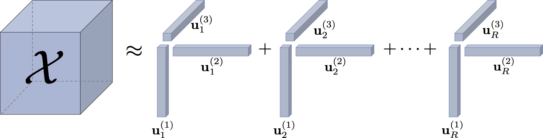
Figure 5: Illustration of a CP decomposition of third-order tensor $\mathcal{{X}}$ into a sum of rank-1 tensors.

IV-B2 Tucker decomposition

The Tucker decomposition [83] decomposes, non-uniquely, $\mathcal{{X}}$ into a core tensor $\mathcal{{G}}\in\mathbb{R}^{R_{1}\times R_{2}\times\cdots\times R_{N}}$ and a set of factor matrices $\left(\mathbf{U}^{(1)},\mathbf{U}^{(2)},\cdots,\mathbf{U}^{(N)}\right)$, with $\mathbf{U}^{(n)}\in\mathbb{R}^{R_{n}\times I_{n}},n=1,2,\ldots,N$ which are multiplied with $\mathcal{{G}}$ along its modes as follows:

$$\mathcal{{X}} =\mathcal{{G}}\times_{1}\mathbf{U}^{(1)}\times_{2}\mathbf{U}^{(2)}\times_{3}\cdots\times_{N}\mathbf{U}^{(N)}.$$ (5)

The core tensor captures interactions between the columns of factor matrices. If $R_{n}\ll I_{n}$, $\forall n$, then the core tensor can be viewed as a compressed version of $\mathcal{{X}}$. It is also worth noting that the CP decomposition can be expressed as Tucker decomposition, with $R_{n}=R$, $\forall n\in\{1,2,\ldots,N\}$ and the core tensor being superdiagonal. The Tucker decomposition is denoted compactly as $\llbracket{}{\mathcal{{G}}};\,{\mathbf{U}^{(1)},\mathbf{U}^{(2)},\cdots,\mathbf{U}^{(N)}}\rrbracket{}$ [34], and it is shown pictorially in Fig. 6. By imposing the factor matrices to be orthonormal, the Tucker model is known as higher-order singular value decomposition (HOSVD) [84].

In practice, data are corrupted by noise, and as in the matrix case, both the Tucker and CP decompositions are not exact. Therefore, they are approximated by optimizing a suitable criterion representing fitting loss. Typically, the least-squares criterion is employed. In this case, assuming that $\{R_{n}\}_{n=1}^{N}$ are known, the Tucker decomposition is computed by solving the following non-convex minimization problem:

$$\min_{\mathcal{{G}},\{\mathbf{U}^{(n)}\}_{n=1}^{N}}\|\mathcal{{X}}-\llbracket{}{\mathcal{{G}}};\,{\mathbf{U}^{(1)},\mathbf{U}^{(2)},\cdots,\mathbf{U}^{(N)}}\rrbracket{}\|^{2}.$$ (6)

The most common optimization algorithm for the Tucker and CP decomposition is the Alternating Least Square (ALS) [85], where the unknowns are estimated iteratively. More specifically, the ALS fixes, sequentially, all but one factor, which is then updated by solving a linear least-squares problem. However, the ALS algorithm is not guaranteed to convergence towards a minimum; see [35] for example.

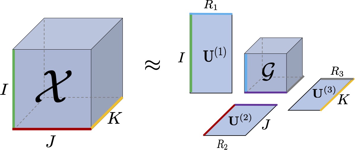
Figure 6: Illustration of a Tucker decomposition of a third-order tensor $\mathcal{{X}}$ into a core tensor and three matrices.

IV-B3 Tensor-Train

The Tensor-Train (TT) decomposition [86], also known as the Matrix-Product-State [87] in quantum physics, expresses $\mathcal{{X}}$ as a product of third order tensors $\mathcal{{G}}_{1}\in\mathbb{R}^{R_{1}\times I_{1}\times R_{2}},\cdots,\mathcal{{G}}_{N}\in\mathbb{R}^{R_{N}\times I_{N}\times R_{N+1}}$ (the cores of the decomposition), such that:

$$\mathcal{{X}}(i_{1},i_{2},\cdots,i_{N})=\underbrace{\mathcal{{G}}_{1}[i_{1}]}_{R_{1}\times R_{2}}\times\underbrace{\mathcal{{G}}_{2}[i_{2}]}_{R_{2}\times R_{3}}\times\cdots\times\underbrace{\mathcal{{G}}_{N}[i_{N}]}_{R_{N}\times R_{N+1}}.$$

The boundary conditions of the tensor-train (open boundary conditions) decomposition dictate $R_{1}=R_{N+1}=1$. The decomposition is illustrated in Fig. 7. The open boundary conditions can be replaced by periodic boundary conditions (the Tensor-Ring) [88, 89] which instead contracts together the first and last cores along $R_{1}$ and $R_{N+1}$.

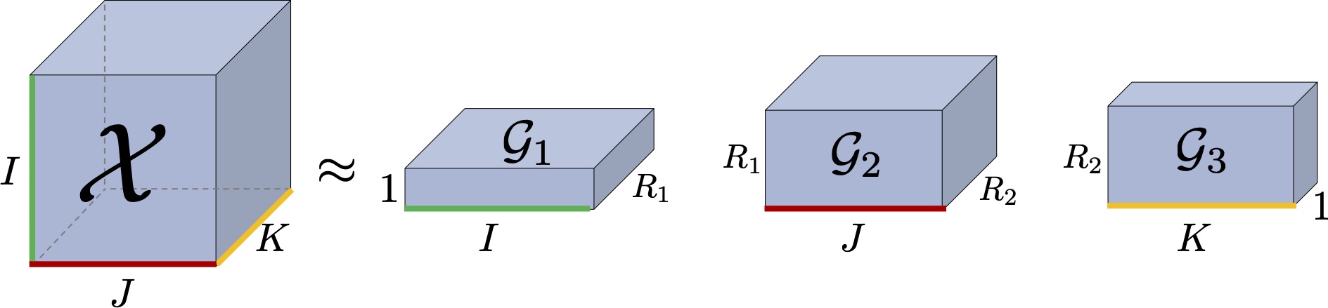
Figure 7: Illustration of a Tensor-Train decomposition of a third-order tensor $\mathcal{{X}}$ into a series of third-order cores. The boundary conditions dictate $R_{1}=R_{N+1}=1$

Let us now depict the aforementioned tensor decompositions using tensor diagrams. While representing tensor decompositions visually (e.g., Figures 5 and 6), we are inherently limited to a maximum of third-order tensors, tensor diagrams conveniently represent decompositions of higher-order tensors. For instance, let $\mathcal{{X}}\in\mathbb{R}^{I_{1}\times I_{2}\times I_{3}\times I_{4}\times I_{5}}$ be a $5^{\text{th}}$-order tensor, its CP decomposition is shown in Fig. 8, Tucker decomposition is shown in Fig. 9, and Fig. 10 depicts its TT decomposition.

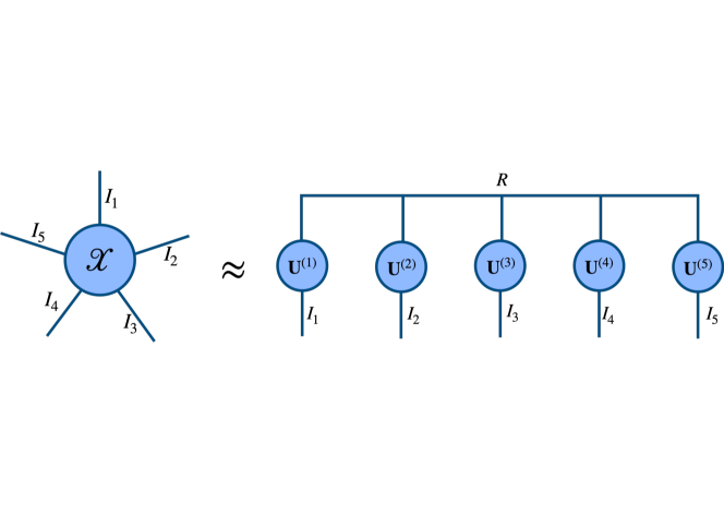
Figure 8: Representation of a CP decomposition using tensor diagrams.

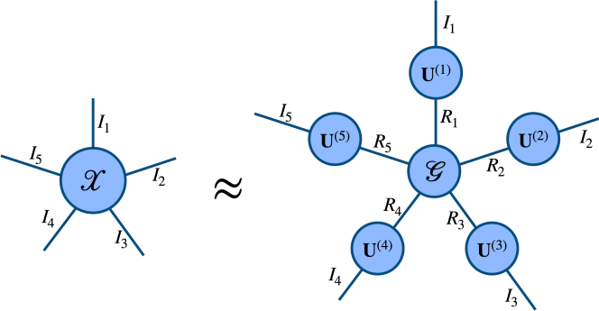
Figure 9: Representation of a Tucker decomposition using tensor diagrams.

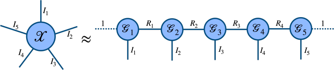
Figure 10: Representation of a Tensor-Train decomposition using tensor diagrams.

IV-C Robust tensor decomposition

Notebook: rpca.ipynb

Visual data of interest, such as facial images captured in unconstrained, real-world conditions, are often severely corrupted by nuisance factors of variation. Such factors include, but are not limited to, significant pose variations, illumination changes, and occlusions, as well as artifacts or missing data introduced during the acquisition process. Collectively, these can be characterized as gross errors. From a statistical point of view, gross errors and outliers do not follow a Gaussian distribution, as is assumed in the vast majority of learning models employed in computer vision–including the tensor decompositions discussed above. Indeed, learning models that rely on optimization of algebraic criteria induced by second-order statistics of observations (e.g., covariance matrix), or goodness of fit measures such as the least-squares criterion, are unable to cope with gross errors and outliers [90]. As a result, the estimated components can be arbitrarily far from the true ones. Hence, their applicability in analyzing visual data captured in unconstrained conditions is rather limited.

Robust tensor decomposition methods aim to recover a low-rank tensor from noisy measurements, assuming the presence of non-Gaussian noise of possibly large magnitude. Those outliers only affect a small fraction of the measurements, and consequently, noise is considered sparse. Concretely, robust tensor modeling seeks a decomposition of the form:

$$\mathcal{{X}}=\mathcal{{L}}+\mathcal{{S}},$$ (7)

where $\mathcal{{X}}$ is an $N^{\text{th}}$-order data tensor usually composed by arranging a set of tensorial data samples of $N-1^{\text{th}}$ order along the $N^{\text{th}}$ mode of the tensor. $\mathcal{{L}}$ and $\mathcal{{S}}$ are unknown $N^{\text{th}}$-order tensors accounting for the low-rank tensor and sparse noise, respectively.

However, as mentioned previously optimizing tensor rank is intractable [78] in general. To address this [91, 92, 93, 94] rely on approximating tensor rank by a convex combination of the n-ranks of $\mathcal{{L}}$. That is, $\sum_{n=1}^{N}\alpha_{n}\operatorname{rank}_{n}(\mathcal{{L}}),$ where $\alpha_{n}\geq 0,\sum_{n=1}^{N}\alpha_{n}=1$ and $\operatorname{rank}_{n}(\mathcal{{L}})$ denotes the column rank of the mode-$n$ matricization of $\mathcal{{L}}$. Therefore, the low-rank tensor is recovered by solving:

$$\min_{\mathcal{{L}},\mathcal{{S}}}\sum_{n=1}^{N}\alpha_{n}\operatorname{rank}_{n}(\mathcal{{L}})+\lambda\|\mathcal{{S}}\|_{0}\quad\text{s.t.}\quad\mathcal{{X}}=\mathcal{{L}}+\mathcal{{S}},$$ (8)

where $\lambda$ is a positive parameter. However, both the $\operatorname{rank}_{n}$ function and the $\ell_{0}$-norm are discrete functions and hence hard to optimize [95, 96]. To make (8) tractable, discrete norms are replaced by their convex surrogates [47, 46]. That is, the rank function is replaced by the nuclear norm and the $\ell_{0}$-norm by the $\ell_{1}$-norm, resulting into a convex optimization problem: [97, 94]:

$$\min_{\mathcal{{L}},\mathcal{{S}}}\sum_{n=1}^{N}\alpha_{n}\|\mathbf{L}_{(n)}\|_{*}+\lambda\|\mathcal{S}\|_{1}\quad\text{s.t.}\quad\mathcal{X}=\mathcal{L}+\mathcal{S},$$ (9)

which is an extension of principal components pursuit (PCP) [75] to higher-order tensors. It is also worth noting that under certain conditions (9) is guaranteed to exactly recover the low-rank component [98]. Similar models has been introduced for the problems of tensor completion [99, 100, 101, 98, 92].

As mentioned in Section IV-B, the CP and Tucker decompositions are approximated in practice by minimizing the least-squares criterion, resulting in algorithms sensitive to sparse, non-Gaussian noise. To alleviate this problem and obtain more robust approximations of tensor decompositions  [102, 103, 94] replace least-squares loss with the $\ell_{1}$-norm.

The vast majority of the aforementioned models are optimized iteratively by employing alternating direction method of multipliers (ADMM) type of algorithms [104].

IV-D Tensor component analysis

Notebooks: MPCA.ipynb, MDA.ipynb

Tensor component analysis (also referred to as multilinear subspace learning [3]) extends the concept of component analysis to data represented by higher-order tensors (please refer to [3, 8] for an overview on the topic).

Let us assume a set of $M$ tensor data samples, that is $\{\mathcal{{X}}_{m}\}_{m=1}^{M}$, where each data sample is a $N-1$-order tensor $\mathcal{{X}}_{m}\in\mathbb{R}^{I_{1}\times I_{2}\times\cdots\times I_{N-1}}$. Therefore, as mentioned previously, a set of such data is represented by an $N^{\text{th}}$ order tensor $\mathcal{{X}}\in\mathbb{R}^{I_{1}\times I_{2}\times\cdots\times I_{N}}$. Tensor component analysis methods seek to estimate a set of $N-1$ projection matrices, $\{\mathbf{U}^{(n)}\in\mathbb{R}^{R_{n}\times I_{n}}\}_{n=1}^{N-1}$ with $R_{n}\ll I_{n}\forall n\in\{1,2,\ldots,N-1\}$ such that the projection of tensor data samples onto the a low-dimensional multilinear subspace, namely $\{\mathcal{{X}}_{m}\times_{1}\mathbf{U}^{(1)}\times_{2}\mathbf{U}^{(2)}\times_{3}\cdots\times_{N-1}\mathbf{U}^{(N-1)}=\mathcal{{X}}_{m}\prod_{n=1}^{N-1}\times_{n}\mathbf{U}^{(n)}\in\mathbb{R}^{R_{1}\times R_{2}\times\cdots\times R_{N-1}}\}_{m=1}^{M}$, yields a low-dimensional tensor representation that satisfy some optimality criterion, such as minimizing reconstruction error e.g., [9] or maximizing tensor scatter [105]. Structural constraints, such as orthogonality in Multilinear PCA (MPCA) [105] or non-negativity in Non-Negative Tensor Factorization (NTF) [9] and its variants [106] are also imposed often on multilinear projections.

Different tensor component analysis methods can be derived as different solutions to constrained optimization problems. For example, unsupervised tensor component analysis can be formulated as a constrained low-rank tensor approximation problem:

$$\min_{\{\mathbf{U}^{(n)}\}_{n=1}^{N}} \|\mathcal{{X}}-\mathcal{{G}}\times_{1}{\mathbf{U}^{(1)}}^{\top}\times_{2}{\mathbf{U}^{(2)}}^{\top}\times_{3}\cdots\times_{N}{\mathbf{U}^{(N)}}^{\top}\|^{2}$$ (10)

$$+\sum_{n=1}^{N}\lambda_{n}r_{n}\left(\mathbf{U}^{(n)}\right)\quad\mbox{s.t.}\;\;\{\mathbf{U}^{(n)}\in\;\;\mathcal{C}_{n}\}_{n=1}^{N},$$

where $r_{n}(\cdot)$ is a regularization function (e.g., $\ell_{1}$-norm for inducing sparsity), $\lambda_{n}$ is a positive regularization parameter, and $\mathcal{C}_{n}$ denotes a set of structural constraints imposed onto the low-dimensional factors. For instance, MPCA [105] is derived by (10) by setting $\mathcal{{G}}=\mathcal{{X}}\times_{1}{\mathbf{U}^{(1)}}\times_{2}{\mathbf{U}^{(2)}}\times_{3}\cdots\times_{N-1}{\mathbf{U}^{(N-1)}}\times_{N}\mathbf{I}$, requiring ${\mathbf{U}^{(N-1)}}=\mathbf{I}$, and enforcing all the $N-1$ projection matrices to be column orthonormal. That is, $\{\mathcal{C}_{n}={\mathbf{U}^{(n)}}^{\top}\mathbf{U}^{(n)}=\mathbf{I}\}_{n=1}^{N-1}$. Furthermore, by requiring factor matrices to be orthogonal and nonnegative (10) yields the non-negative MPCA [107]. By neglecting orthogonality constraints and requiring factor matrices to be only nonnegative, i.e., $\{\mathcal{C}_{n}=\mathbf{U}^{(n)}\geq\mathbf{0}\}_{n=1}^{N-1}$ the NTF [9] is obtained by (10) when $\mathcal{{G}}$ is a superdiagonal tensor, i.e., $\mathcal{{G}}=\mathcal{{I}}$.

Supervised tensor component analysis exploits available side information such as class labels or neighborhood relationships among samples to estimate a multilinear projection. Such models can be unified under the graph embedding framework [74] by solving:

$$\min_{\{\mathbf{U}^{(n)}\}_{n=1}^{N-1}} \sum_{m,k\atop m\neq k}^{M}\mathbf{W}_{m,k}\|\mathcal{{X}}_{m}\prod_{n=1}^{N-1}\times_{n}\mathbf{U}^{(n)}-\mathcal{{X}}_{k}\prod_{n=1}^{N-1}\times_{n}\mathbf{U}^{(n)}\|^{2},$$ (11)

$$\mbox{s.t}\quad\sum_{m,k}^{M}\mathbf{B}_{m,k}\|\mathcal{{X}}_{m}\prod_{n=1}^{N-1}\times_{n}\mathbf{U}^{(n)}\|^{2}=1,$$

where $\mathbf{W}$ denotes the affinity matrix capturing some sort of within-class neighborhood relationship among tensor samples $\mathcal{{X}}_{m}$ and $\mathbf{B}$ is an affinity matrix representing between-class neighborhood relationship. Multilinear extensions to Linear Discriminant Analysis (LDA), such as [108, 109, 110] for example, are obtained by setting $\mathbf{W}_{mk}=\delta_{c_{m},c_{k}}/n_{c_{m}}$ and $\mathbf{B}=\mathbf{I}-\frac{1}{M}\mathbf{e}\mathbf{e}^{\top}$, where $\delta$ denotes the Kronecker delta function, $\mathbf{e}$ is the standard basis and $n_{c}$ denotes the number of the samples belonging to the $c^{\text{th}}$ class.

IV-E Tensor-structured dictionary learning

Sparse coding (or dictionary learning) methods are central in numerous visual information processing tasks. In this context, a data matrix $\mathbf{X}\in\mathbb{R}^{I\times M}$ contains in its columns vectorized image patches of size $\sqrt{I}\times\sqrt{I}$, rather than data samples. Assuming $\mathbf{D}$ is over-complete and requiring $\mathbf{R}=[\mathbf{r}_{1},\mathbf{r}_{2},\ldots,\mathbf{r}_{M}]$ to be sparse, sparse dictionary learning solves the following, non-convex, optimization problem:

$$\min_{\mathbf{R},\mathbf{D}}\|\mathbf{X}-\mathbf{D}\mathbf{R}\|_{F}^{2}+\lambda\sum_{m=1}^{M}\|\mathbf{r}_{m}\|_{0},$$ (12)

However, extracting patches from images and flattening them into vectors makes (12) suboptimal for multidimensional tensor data. Besides structure loss, typical solvers for (12), such as the K-SVD family of algorithms [65], suffer from a high computational burden, preventing their applicability to massive amounts of tensor data.

To preserve multilinear structures in dictionary learning, a separable structure on the dictionary can be enforced. For instance, Separable Dictionary Learning (SeDiL) [11] considers a set of samples in matrix form, namely, $\{\mathbf{X}_{m}\}_{m=1}^{M}$, admitting sparse representations on a pair of bases $\mathbf{U}^{(1)},\mathbf{U}^{(2)}$, of which the Kronecker product constructs the dictionary. More specifically, SeDiL solves:

$$\min_{\mathbf{U}^{(1)},\mathbf{U}^{(2)},\mathcal{{R}}} \frac{1}{2}\sum_{m=1}^{M}\|\mathbf{X}_{m}-\mathbf{U}^{(1)}\mathbf{R}_{m}{\mathbf{U}^{(2)}}^{\top}\|_{F}^{2}$$

$$+\lambda_{1}g(\mathcal{{R}})+\lambda_{2}r(\mathbf{U}^{(1)})+\lambda_{3}r(\mathbf{U}^{(2)}),$$ (13)

where the regularizers $g(\cdot)$ and $r(\cdot)$ promote sparsity in the representations, and low mutual-coherence of the dictionary $\mathbf{D}=\mathbf{U}^{(2)}\otimes\mathbf{U}^{(1)}$, respectively. Here, $\mathbf{D}$ is constrained to have orthogonal columns.

A different approach is taken in [111], where a separable 2D dictionary is learned following a two-step strategy similar to that of the K-SVD. Each observation matrix $\mathbf{X}_{m}$ is approximated by $\mathbf{U}^{(1)}\mathbf{R}_{m}{\mathbf{U}^{(2)}}^{\top}$, where $\mathbf{R}_{m}$ are slices of a core tensor $\mathcal{{R}}$. In the first step, the sparse representations $\mathbf{R}_{m}$ are obtained by 2D Orthogonal Matching Pursuit (OMP) [112]. In the second step, a CP decomposition is performed on a tensor of residuals.

Theoretical analysis suggests that the sample complexity of tensor-structured dictionary learning can be significantly lower than that for unstructured, vector data; see [113] for 2D data, and [114] for $N$-order tensor data. This suggests better performance is achievable with separable dictionary learning from tensor data compared to vector-based dictionary learning methods.

However, the aforementioned models learn dictionaries on many small image patches whose number can easily become prohibitively large, undermining the scalability benefits of learning separable dictionaries. Moreover, it is worth noting that none of the models mentioned above are robust to gross errors due to the loss function used. Such limitations are alliviated by the Robust Kronecker Component Analysis (RKCA) [115, 4].

The RKCA combines ideas from separable dictionary learning and robust tensor decomposition. Instead of seeking overcompleteness, low-rank is promoted on the pair of dictionaries, and sparsity is imposed in the code yielding a sparse representation of the input tensor samples. Specifically, RKCA solves:

$$\min_{\mathbf{U}^{(1)},\mathbf{U}^{(2)},\mathcal{{R}},\mathcal{{S}}}\sum_{m=1}^{M}\|\mathbf{X}_{m}-\mathbf{U}^{(1)}\mathbf{R}_{m}{\mathbf{U}^{(2)}}^{\top}-\mathbf{S}_{m}\|_{F}^{2}$$

$$+\lambda\sum_{m=1}^{M}\|\mathbf{R}_{m}\|_{1}+\lambda\sum_{m=1}^{M}\|\mathbf{S}_{m}\|_{1}+\|\mathbf{U}^{(2)}\otimes\mathbf{U}^{(1)}\|_{F},$$ (14)

where matrices $\{\mathbf{S}_{m}\}_{m=1}^{M}$ account for sparse noise and outliers. Equivalently, enforcing the equality constraints and concatenating the matrices $\mathbf{X}_{m}$, $\mathbf{R}_{m}$, and $\mathbf{S}_{m}$ as the frontal slices of a third-order tensor, (IV-E) is written as:

$$\min_{\mathbf{U}^{(1)},\mathbf{U}^{(2)},\mathcal{{R}},\mathcal{{S}}} \alpha\|\bm{\mathcal{R}}\|_{1}+\lambda\|\mathcal{S}\|_{1}+\|\mathbf{U}^{(2)}\otimes\mathbf{U}^{(1)}\|_{\mathrm{F}}$$

s.t $$\mathcal{X}=\mathcal{R}\times_{1}\mathbf{U}^{(1)}\times_{2}\mathbf{U}^{(2)}+\mathcal{S}.$$ (15)

Consequently, (IV-E) indicate that separable dictionary can be expressed as a regularized tensor decomposition. As opposed to classic dictionary learning models, it is worth mentioning that following [116, 117], the global optimality of RKCA is ensured.

IV-F Tensor regression

Besides learning representations, low-rank tensor decomposition facilitates reducing the parameters of tensor regression models and prevents overfitting. Tensor regression models generalize linear regression to higher-order tensors. More specifically, in tensor regression a regression output $y\in\mathbb{R}$ is expressed as the inner product between the observation tensor $\mathcal{{X}}$ and a weight tensor $\mathcal{{W}}$ with the same dimension as $\mathcal{{X}}$: $y=\langle{\mathcal{{X}}},{\mathcal{{W}}}\rangle+b$. Several low-rank tensor regression models have been proposed [5, 118, 119, 120, 121, 122]. These methods share the assumption that the unknown regression weight tensor is low-rank. This is enforced by expressing the weights tensor in CP [5, 119] or Tucker form [123, 121, 124]. Alternatively, low-rank constraints on the weight tensor are enforced by spectral regularization, such as applying the nuclear norm on the unfoldings of the weight tensor along its modes [123], in a similar way to robust tensor decomposition described in Section IV-C. To further prevent overfitting, regularization is incorporated into low-rank tensor regression models. For instance, [120, 5, 118] employ tensor norm and hence extend the low-rank ridge regression to high-order tensors. $\ell_{1}$-norm and elastic-net regularization is adopted in [119], while a combination of $\ell_{1}$-norm and nuclear norm regularizes the weight tensor in [122] forcing it to be simultaneously low-rank and sparse. It is worth mentioning that low-rank regression models extend support vector machines to higher-order tensors, e.g., [5, 122].

Furthermore, higher-order generalizations of Partial-Least Squares were proposed [125, 126]. The idea of Higher Order Partial Least Squares (HO-PSL) is to find a latent correlated subspace between the observation tensor and the response tensors. Alternatively, it is possible to perform regression in a subspace obtained with Tensor PCA [127]. Finally, quantile regression has also recently been generalized to higher-order [128], using a Tucker structure on the regression weights.

V Tensor Methods in Deep Neural Networks Architectures

Tensors play a central role in modern deep learning architectures. The basic building blocks of deep neural networks, such as multichannel convolutional kernels and attention blocks, are essentially tensor mappings, represented by tensors. Deep neural networks, as mentioned earlier, operate in a regime where the number of parameters is typically tens of millions or even billions, and is thus much larger than the number of training data. In this over-parameterized regime, incorporating tensor decompositions into deep learning architectures leads to a significant reduction in the number of unknown parameters. This allows the design of networks that further preserve the topological structure in the data, being more parsimonious in terms of parameters, more data-efficient, and more robust to various types of noise and domain shifts. Besides the design of deep networks, tensor analysis can be beneficial in demystifying the success behind neural networks, having already been used to prove universal approximation properties of neural networks [129], or to understand the inductive bias leveraged by networks in computer vision [130]. This section overviews recent developments in the use of tensor methods to design efficient and robust deep neural networks and the theoretical understanding of their properties.

V-A Parameterizing fully-connected layers

Notebook: tt-compression.ipynb

Leveraging tensor decompositions within neural networks by re-parametrizing fully-connected layers has been first proposed in [21]. Since the weights of fully-connected layers are represented as matrices, tensor decompositions cannot be applied directly. Therefore, the weight matrix needs to be reshaped to obtain a higher-order tensor.

Specifically, consider an input matrix $\mathbf{W}$ of size $I\times J$, whose dimensions can be expressed as $I=I_{1}\times I_{2}\times\cdots\times I_{N}$ and $J=J_{1}\times J_{2}\times\cdots\times J_{N}$. Hence, $\mathbf{W}$ is tensorized first by reshaping it to a higher-order tensor of size $I_{1}\times I_{2}\times\cdots\times I_{N}\times J_{1}\times J_{2}\times\cdots\times J_{N}$. Next, by permuting the dimensions and reshaping it again, an $N$${}^{\text{th}}$ order tensor of $I_{1}J_{1}\times I_{2}J_{2}\times\cdots\times I_{N}J_{N}$ is obtained. This tensor is then compressed in the TT format. The approximated weights are reconstructed from that low-rank TT factorization during inference, and are then reshaped back into a matrix.

In this setting, other types of decompositions have also been explored, including Tensor-Ring [131] and Block-Term Decomposition [132]. This strategy has also been extended to parametrize other types of layers [133].

In the context of two-layer fully-connected neural networks, tensors have also been used for deriving alternative to (stochastic) gradient descent methods for training, with guaranteed generalization bounds. Specifically, in [134], the CP decomposition is applied on the cross-moment tensor, which encodes the correlation between the third-order score function (i.e., the normalized derivative of the input pdf) to obtain the parameters of the first layer. The parameters of the second layer are obtained next via regression. Under mild assumptions, this approach comes with guaranteed risk bounds in both the realizable setting (i.e., the target function can be approximated with zero error from the neural network under consideration) and the non-realizable one, where the target function is arbitrary.

V-B Tensor contraction layers

In modern deep neural networks such as CNNs, each layer’s output is an (activation) tensor. However, activation tensors are usually flattened and passed to subsequent fully-connected layers resulting in structural information loss. A natural way to preserve the multilinear structure of activation tensors is to incorporate tensor operations into deep networks. For instance, tensor contraction can be applied to an activation tensor to obtain a low-dimensional representation of it [24]. In other words, an input activation tensor is contracted along each mode with a projection matrix (an n-mode product as defined earlier).

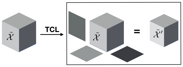
Figure 11: An input tensor $\mathcal{{X}}$ is contracted into a smaller tensor $\mathcal{{X^{\prime}}}$ through a Tensor Contraction Layer [24].

Let us assume a network involves an input activation tensor $\mathcal{{X}}$ of size $S\times I_{1}\times\cdots\times I_{N}$, where $S$ is the batch size. A Tensor Contraction Layer (TCL) contracts the input activation tensor, along each of its dimensions except the batch-size, with a series of factor matrices $\{\mathbf{V}^{(n)}\}_{n=2}^{N}$.The result is a compact core tensor $\mathcal{{X^{\prime}}}$ of smaller size $S\times R_{1}\times\cdots\times R_{N}$ defined as

$$\mathcal{{X^{\prime}}}=\mathcal{{X}}\times_{2}\mathbf{V}^{(2)}\times_{3}\mathbf{V}^{(3)}\times\cdots\times_{N}\mathbf{V}^{(N)},$$ (16)

with $\mathbf{V}^{(n)}\in\mathbb{R}^{R_{n}\times I_{n}},n\in[{2}\mathrel{{.}\,{.}}\nobreak{N}]$. Note that the projections start at the second mode as we do not contract along the first mode $S$, which corresponds to the mini-batch size. These factors are learned in an end-to-end manner, concurrently with all the other network parameters by gradient backpropagation. A TCL that produces a compact core of smaller size is denoted as size–$\left(R_{2},\cdots,R_{N}\right)$ TCL, or TCL–$\left(R_{2},\cdots,R_{N}\right)$.

In addition to preserving the multi-linear structure in the input, TCLs have much less parameters than a corresponding fully-connected layer. We can see this by establishing the link between a fully-connected layer with structured weights and a tensor regression layer. Let us assume an input activation tensor $\mathcal{{X}}$ of size $S_{1}\times I_{1}\times\cdots\times I_{N}$. A size–$\left(R_{2},\cdots,R_{N}\right)$ TCL parameterized by weight factors $\mathbf{V}^{(2)},\cdots,\mathbf{V}^{(N)}$ has a total of $\sum_{n=2}^{N}I_{n}\times R_{n}$ parameters. By unfolding the input tensor (i.e., vectorizing each sample of the batch), TCL can be equivalently expressed as a fully-connected layer parametrized by the weight matrix $\mathbf{W}=\left(\mathbf{V}^{(2)}\otimes\cdots\otimes\mathbf{V}^{(N)}\right)^{\top}$, which computes

$$\mathcal{{X}}_{[1]}\mathbf{W}=\mathcal{{X}}_{[1]}\left(\mathbf{V}^{(2)}\otimes\cdots\otimes\mathbf{V}^{(N)}\right)^{\top}.$$

However, since fully-connected layers have no structure on their weights, the corresponding fully-connected layer parametrized by a weight matrix $\mathbf{W}$ of the same size as above would have a total of $\prod_{n=2}^{N}I_{n}\times R_{n}$ parameters, compared to the $\sum_{n=2}^{N}I_{n}\times R_{n}$ parameters of the TCL.

V-C Tensor regression layers

Notebook: tensor_regression_layer.ipynb

In CNNs, after an activation tensor has been obtained through a series of convolutional layers, predictions (outputs) are typically generated by flattening this activation tensor or applying a spatial pooling, before using a fully-connected output layer. However, both approaches discard the multilinear structure of the activation tensor. To alleviate this, tensor regression models can be incorporated within deep neural networks and trained end-to-end jointly with the other parameters of the network [25].

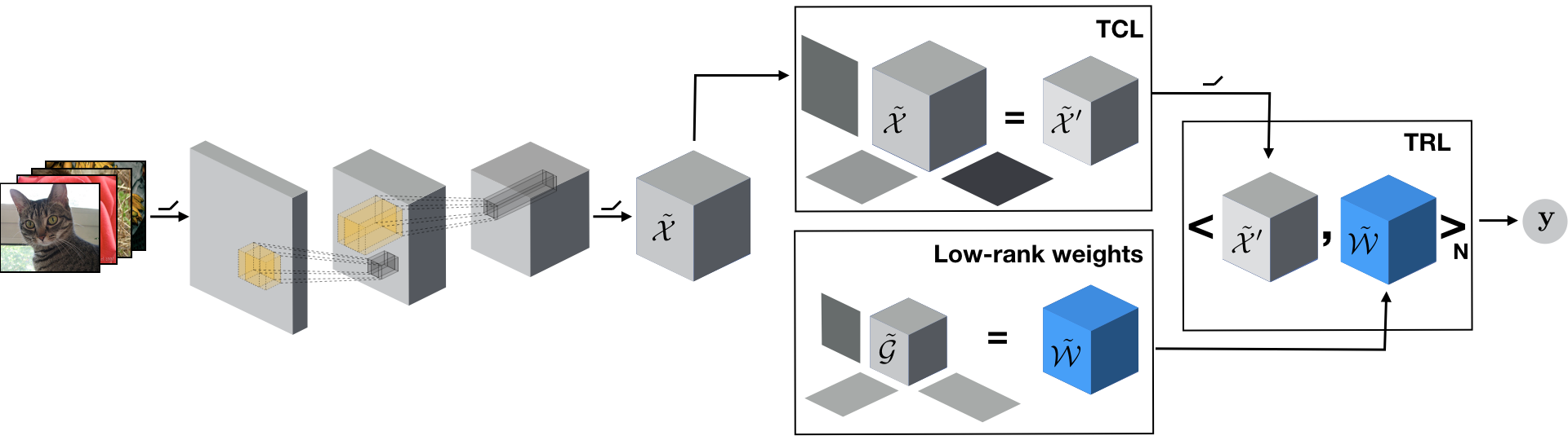
Figure 12: Illustration of a convolutional deep network where the activation tensor is processed through a TCL followed by a TRL to produce the outputs while preserving the topological structure [25]. Note that $y$, here, is a scalar.

Specifically, let us assume we have a set of $S$ input activation tensors $\mathcal{{X}}^{(s)}\in\mathbb{R}^{I_{1}\times I_{2}\times\cdots\times I_{N}}$ and corresponding target labels $y^{(s)}\in\mathbb{R}$, with $s\in[{1}\mathrel{{.}\,{.}}\nobreak{S}]$. A Tensor Regression Layer (TRL) estimates the regression weight tensor $\mathcal{{W}}\in\mathbb{R}^{I_{1}\times I_{2}\cdots\times I_{N}},$ by further assuming that it admits a low-rank decomposition. Originally, TRL has been introduced by assuming a Tucker structure on the regression weights. That is, for a rank–$\left(R_{1},\cdots,R_{N}\right)$ Tucker decomposition, we have:

$$y^{(s)} =\langle{\mathcal{{X}}^{(s)}},{\mathcal{{W}}}\rangle+b$$

with $$\mathcal{{W}}=\mathcal{{G}}\times_{1}\mathbf{U}^{(1)}\times_{2}\mathbf{U}^{(2)}\cdots\times_{N}\mathbf{U}^{(N)}$$ (17)

with $\mathcal{{G}}\in\mathbb{R}^{R_{1}\times\cdots\times R_{N}}$, $\mathbf{U}^{(n)}\in\mathbb{R}^{I_{n}\times R_{n}}$ for each $n$ in $[{1}\mathrel{{.}\,{.}}\nobreak{N}]$ and $\mathbf{U}^{(N)}\in\mathbb{R}^{1\times R_{N}}$. For simplicity, here, we introduce the problem for a scalar output, but it is established, in general, for a tensor-valued response. The inner product between the activation tensor and the regression weight is then replaced by a tensor contraction along matching modes.

In addition to the implicit regularization induced by the low-rank structure of the regression weights, TRLs result in a much smaller number of parameters. For an input activation tensor $\mathcal{{X}}\in\mathbb{R}^{S\times I_{1}\times I_{2}\times\cdots\times I_{N}}$, a rank-$(R_{1},R_{2},\cdots,R_{N},R_{N+1})$ TRL and an $d$-dimensional output. A fully connected layer taking the same input $\mathcal{{X}}$ (after a flattening layer) would have $n_{\text{FC}}$ parameters, with $n_{\text{FC}}=d\times\prod_{n=1}^{N}I_{n}.$ By comparison, a rank-$(R_{1},R_{2},\cdots,R_{N},R_{N+1})$ TRL taking $\mathcal{{X}}$ as input has a number of parameters $n_{\text{TRL}}$, with:

$$n_{\text{TRL}}=\prod_{n=1}^{N+1}R_{n}+\sum_{n=1}^{N}R_{n}\times I_{n}+R_{N+1}\times d.$$

As previously observed for the TCL, TRL is much more parsimonious in terms of the number of parameters. Note that, while we introduced the TRL here with a Tucker structure on the regression weight tensor, in general, any low-rank format can be used, including CP and TT [135].

V-D Parametrizing convolutional layers

The weights of convolutional layers are naturally represented as tensors. For instance, a 2D convolution is represented by a 4${}^{\text{th}}$–order tensor. Hence convolutional layers can directly be compressed by employing tensor decomposition. In fact, there is a close link between deep neural networks and efficient convolutional blocks, which we will highlight in this section.

V-D1 $1\times 1$ convolutions

The first thing to notice is that $1\times 1$ convolutions are tensor contractions. This type of convolution is frequently used within deep neural networks in order to create a data bottleneck. For a $1\times 1$ convolution $\Phi$, defined by kernel $\mathcal{{W}}\in\mathbb{R}^{T\times C\times 1\times 1}$ and applied to an activation tensor $\mathcal{{X}}\in\mathbb{R}^{C\times H\times W}$. We denote the squeezed version of $\mathcal{{W}}$ along the first mode as $\mathbf{W}\in\mathbb{R}^{T\times C}$. We then have:

$$\Phi(\mathcal{{X}})_{t,y,x}=\mathcal{{X}}\star\mathcal{{W}}=\sum_{k=1}^{C}\mathcal{{W}}_{t,k,y,x}\mathcal{{X}}_{k,y,x}=\mathcal{{X}}\times_{1}\mathbf{W}.$$

Note that, here, we have $x=y=1$ as we are considering a $1\times 1$ convolution.

V-D2 Kruskal convolutions

Let us now focus on how tensor decomposition can be applied to the convolutional kernels of CNNs and how this results not only in fewer parameters but also faster operations. The CP decomposition, for instance, allows separating the modes of a convolutional kernel, resulting in a Kruskal form. Albeit the application of tensor decomposition in the context of CNNs is relatively new and of practical interest nowadays, the idea of separable representation of linear operators by means of tensor decomposition is not new (see [136]) and in fact was one of the original motivations for tensor rank decomposition of the matrix-multiplication tensor (see [137] for example).

In computer vision, the use of separable convolutions was proposed in [138], in the context of learnable filter banks. In the context of deep learning, [139] proposed to leverage redundancies across channels by exploiting separable convolutions. Furthermore, it is possible to start from a pre-trained convolutional kernel and apply CP decomposition to it in order to obtain a separable convolution. This was proposed for 2D convolutions in [22], where a CP decomposition of the kernel was achieved by minimizing the reconstruction error between the pre-trained weights and the corresponding CP approximation. The authors demonstrated both space savings and computational speedups. Similar results can be obtained using different optimization strategies such as the tensor power method [23].

An advantage of factorizing the kernel using a CP decomposition is that the resulting factors can be used to parametrize a series of efficient depthwise separable convolutions, replacing the original convolution [22], as illustrated in Fig. 13. This can be seen by considering the expression of a regular convolution:

$$\mathcal{{F}}_{t,y,x}=\leavevmode\color[rgb]{0,0,1}\sum_{k=1}^{C}\leavevmode\color[rgb]{1,0,0}\sum_{j=1}^{H}\leavevmode\color[rgb]{0,1,0}\sum_{i=1}^{W}\mathcal{{W}}(t,\leavevmode\color[rgb]{0,0,1}k,\leavevmode\color[rgb]{1,0,0}j,\leavevmode\color[rgb]{0,1,0}i)\mathcal{{X}}(\leavevmode\color[rgb]{0,0,1}k,\leavevmode\color[rgb]{1,0,0}j+y,\leavevmode\color[rgb]{0,1,0}i+x).$$ (18)

A Kruskal convolution is obtained by expanding the kernel $\mathcal{{W}}$ in the CP form as introduced in Section IV-B1. By reordering the terms, we can then obtain an efficient reparametrization [22]:

$$\mathcal{{F}}_{t,y,x}=\underbrace{\sum_{r=1}^{R}\mathbf{U}^{(T)}_{t,r}\underbrace{\left[\leavevmode\color[rgb]{0,1,0}\sum_{i=1}^{W}\mathbf{U}^{(W)}_{\leavevmode\color[rgb]{0,1,0}i,r}\underbrace{\left(\leavevmode\color[rgb]{1,0,0}\sum_{j=1}^{H}\mathbf{U}^{(H)}_{\leavevmode\color[rgb]{1,0,0}j,r}\underbrace{\left[\leavevmode\color[rgb]{0,0,1}\sum_{k=1}^{C}\mathbf{U}^{(C)}_{\leavevmode\color[rgb]{0,0,1}k,r}\mathcal{{X}}(\leavevmode\color[rgb]{0,0,1}k,\leavevmode\color[rgb]{1,0,0}j+y,\leavevmode\color[rgb]{0,1,0}i+x)\right]}_{\leavevmode\color[rgb]{0,0,1}1\times 1\text{ conv}}\right)}_{\leavevmode\color[rgb]{1,0,0}\text{ depthwise conv}}\right]}_{\leavevmode\color[rgb]{0,1,0}\text{ depthwise conv}}}_{1\times 1\text{ convolution}}$$ (19)

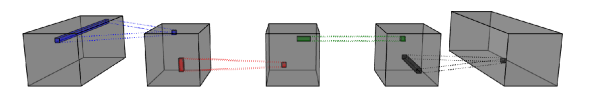
Figure 13: Illustration of a 2D Kruskal convolution, as expressed Eq. 19, with matching colours. First, a $1\times 1$ convolution reduces the number of input channels to the rank (blue). Two depthwise convolutions are then applied on the height and width of the activation tensor (red and green). Finally, a second $1\times 1$ convolution restores the number of channels from the rank of the CP decomposition to the desired number of output channels (black).

V-D3 Tucker convolutions

As previously, we consider the convolution $\mathcal{{F}}=\mathcal{{X}}\star\mathcal{{W}}$ described in (18). However, instead of a Kruskal structure, the convolution kernel $\mathcal{{W}}$ is assumed to admit a Tucker decomposition as follows:

$$\mathcal{{W}}(t,s,j,i)=\sum_{r_{1}=0}^{R_{1}}\sum_{r_{2}=0}^{R_{2}}\sum_{r_{3}=0}^{R_{3}}\sum_{r_{4}=0}^{R_{4}}\mathcal{{G}}_{r_{1},r_{2},r_{3},r_{4}}\mathbf{U}^{(T)}_{t,r_{1}}\mathbf{U}^{(C)}_{s,r_{2}}\mathbf{U}^{(H)}_{j,r_{3}}\mathbf{U}^{(W)}_{i,r_{4}}.$$

This approach allows for an efficient reformulation [140]: first, the factors along the spatial dimensions are absorbed into the core by writing $\mathcal{{H}}=\mathcal{{G}}\times_{3}\mathbf{U}^{(H)}_{j,r_{3}}\times_{4}\mathbf{U}^{(W)}_{i,r_{4}}.$ By reordering the term, we can now see that a Tucker convolution is equivalent to first transforming the number of channels, then applying a (small) convolution before restoring the channel dimension from the rank to the target number of channels:

$$\mathcal{{F}}_{t,y,x}=\underbrace{\leavevmode\color[rgb]{0,1,0}\sum_{r_{1}=1}^{R_{1}}\mathbf{U}^{(T)}_{t,\leavevmode\color[rgb]{0,1,0}r_{1}}\left[\underbrace{\leavevmode\color[rgb]{1,0,0}\sum_{j=1}^{H}\sum_{i=1}^{W}\sum_{r_{2}=1}^{R_{2}}\mathcal{{H}}_{\leavevmode\color[rgb]{0,1,0}r_{1},\leavevmode\color[rgb]{1,0,0}r_{2},\leavevmode\color[rgb]{1,0,0}j,\leavevmode\color[rgb]{1,0,0}i}\left[\underbrace{\leavevmode\color[rgb]{0,0,1}\sum_{k=1}^{C}\mathbf{U}^{(C)}_{\leavevmode\color[rgb]{0,0,1}k,\leavevmode\color[rgb]{1,0,0}r_{2}}\mathcal{{X}}(\leavevmode\color[rgb]{0,0,1}k,\leavevmode\color[rgb]{1,0,0}j+y,\leavevmode\color[rgb]{1,0,0}i+x)}_{\leavevmode\color[rgb]{0,0,1}1\times 1\text{ conv}}\right]}_{\leavevmode\color[rgb]{1,0,0}H\times W\text{ conv}}\right]}_{\leavevmode\color[rgb]{0,1,0}1\times 1\text{ conv}}.$$ (20)

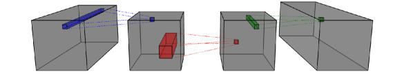
Figure 14: Illustration of a Tucker convolution expressed as a series of small, efficient convolutions, as illustrated in Eq. 20. Note that this is the approach taken by ResNet for the Bottleneck blocks. After the full kernel has been decomposed, the factors along the input and output channels are used to parametrize $1\times 1$ convolutions, applied respectively first (blue) and last (green). The remaining two factors are absorbed into the core and used to parametrize a regular 2D convolution (red).

Besides the aforementioned types of convolutions (i.e., bottleneck layers, separable convolutions), [141] identify maximally resource-efficient convolutional layers utilizing tensor networks and decompositions. Tensor decompositions have also been used for unifying different successful architectures. Particularly, in [29], the block term decomposition [142] is used to unify different architectures that employ residual connections, such as ResNet [15], while proposing a new architecture that improves parameter efficiency. This implies that searching over the space of tensor decompositions and their parameters might be an excellent proxy task to limit the search space for architecture search.

From a theoretical point of view, by using the CP decomposition to replace convolutional with low-rank layers results in deriving the upper bound for the generalization error of the compressed network [143]. This bound improves previous results on the compressibility and generalizability of neural networks [144]. It is also related to the layers’ rank, providing insights on designing neural networks (with low-rank tensors as layers).

V-D4 Multi-stage compression

The factorization strategies mentioned above allow for efficient compression of pre-trained fully-connected and convolutional layers of deep neural networks by applying tensor decomposition to the learned weights. Fine-tuning allows recovery for loss of performance when increasing the compression ratio. However, it is also possible to apply multi-state compression [145] to further compress without loss of performance. Instead of compressing then fine-tuning, the idea is to adopt an iterative approach by alternating low-rank factorization with rank selection and fine-tuning.

V-D5 General N-D separable convolutions and transduction

Design of general (N-dimensional) fully separable, convolution has been introduced in the context of deep neural networks in [27]. Let us assume an $(N+1)^{\text{th}}$–order input activation tensor $\mathcal{{X}}\in\mathbb{R}^{C\times D_{1}\times\cdots\times D_{N}}$ corresponding to $N$ dimensions with $C$ channels. The higher-order separable convolution, which we denote $\Phi$, is defined by a kernel $\mathcal{{W}}\in\mathbb{R}^{T\times C\times K_{1}\times\cdots\times K_{N}}$. By expressing this kernel in a factorized Kruskal form as $\mathcal{{W}}=\llbracket{}{\mathbf{\lambda};\,\,\mathbf{U}^{(T)},\mathbf{U}^{(C)},\mathbf{U}^{(K_{1})},\cdots,\mathbf{U}^{(K_{N})}}\rrbracket{}$, we obtain:

$$\begin{split}\Phi(\mathcal{{X}})_{t,i_{1},\cdots,i_{N}}&=\sum_{r=1}^{R}\sum_{s=1}^{C}\sum_{i_{1}=1}^{K_{1}}\cdots\\ &\cdots\sum_{i_{N}=1}^{K_{N}}\lambda_{r}\bigl{[}\mathbf{U}^{(T)}_{t,r}\mathbf{U}^{(C)}_{s,r}\mathbf{U}^{(K_{1})}_{i_{1},r}\cdots\mathbf{U}^{(K_{N})}_{i_{N},r}\mathcal{{X}}_{s,i_{1},\cdots,i_{N}}\bigr{]}.\end{split}$$

The separable higher-order convolution can be obtained by reordering the term into:

$$\mathcal{{F}}=\left(\rho\left(\mathcal{{X}}\times_{1}\mathbf{U}^{(T)}\right)\right)\times_{1}\left(\operatorname*{diag}(\mathbf{\lambda})\mathbf{U}^{(C)}\right),$$ (21)

where $\rho$ applies the 1D spatial convolutions:

$$\rho(\mathcal{{X}})=\left(\mathcal{{X}}\star_{1}\mathbf{U}^{(K_{1})}\star_{2}\mathbf{U}^{(K_{2})}\star\cdots\star_{N}\mathbf{U}^{(K_{N})}\right).$$ (22)

A factorized separable convolution can be extended from $N$-dimensions to $N+K$ ($N,K\in\mathbb{N}$) by means of transduction [27]. Since the convolution is fully separable, it is possible to add additional factors. In particular, to apply transduction from $N$ to $N+1$, it is sufficient to add an additional factor $\mathbf{U}^{K_{N+1}}$ and update $\rho$ in equation (22) to:

$$\rho(\mathcal{{X}})=\left(\mathcal{{X}}\star_{1}\mathbf{U}^{(K_{1})}\star_{2}\mathbf{U}^{(K_{2})}\star\cdots\star_{N}\mathbf{U}^{(K_{N})}\star_{N+1}\mathbf{U}^{(K_{N+1})}\right).$$

V-D6 Parametrizing full networks

So far, we reviewed methods focusing on parametrizing a single layer. It is also possible to jointly parametrize a whole convolutional neural network with a single low-rank tensor. This is the idea of “T-Net” [26], where all the convolutional layers of a stacked-hourglass [146] (a type of U-Net [147]) are parametrized by a single 8${}^{\text{th}}$–order tensor. Each of the modes of this tensor models a modality of the network, allowing to jointly model and regularize all the layers. Hence correlations across channels, layers, convolutional blocks, and subnetworks of the model can be leveraged. Imposing low-rank constraints on this model tensor results in large parameter space savings with little to no impact on performance, or even improved performance, depending on the compression ratio. That is, small compression ratios result in improved performance, while it is possible to reach substantial compression ratios with only minor decreases in performance. In addition, it is possible to partially reconstruct the full tensor to obtain a Tucker factorization of the kernel of each layer, thus allowing for speedups as described in section V-D3.

V-D7 Preventing degeneracies in factorized convolutions

As we discussed above, when parametrizing DCNNs, one can either train the factorized layers from scratch in an end-to-end fashion via stochastic gradient descent, or decompose existing convolutional kernels to obtain the factorized version. In the latter case, the authors of [148] showed that when applying decomposition to obtain a factorized convolution, degeneracy can appear in the decomposition due to diverging components. They tackle this issue and enable stable factorization of convolutional layers through sensitivity minimization.

V-E Robustness of deep networks

Deep neural networks produce remarkable results in computer vision applications but are typically very vulnerable to noise, such as capture noise, corruption, adversarial attacks of domain shift. Below, we provide a brief review of tensor methods that robustify deep networks.

V-E1 Tensor Dropout

One known way to increase robustness is to incorporate randomization during training. For example, Dropout [149] randomly drops activations, while DropConnect [150] applies the randomization to the weights of fully-connected layers. However, randomizing directly in the original space results in sparse weights or activations (with zero-ed values), which affects the high-order statistics.

Tensor dropout [33] is a principled way to incorporate randomization to robustify the model without altering its statistics. It consists of applying sketching matrices in the latent subspace spanned by a tensor decomposition, whether that’s CP (see Fig. 15) or Tucker (see Fig. 16), leading to significantly improved robustness to random noise (e.g., during capture) or adversarial attacks.

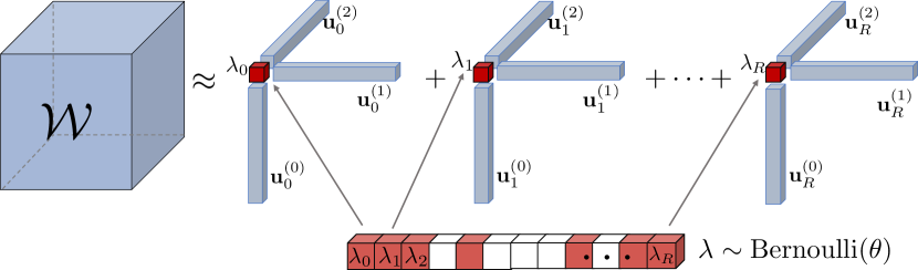
Figure 15: Tensor Dropout on a CP decomposition. Visualization of tensor dropout applied to a CP factorization. Here, a Bernouilli dropout is applied by first sampling a multivariate Bernoulli random vector $\mathbf{\lambda}$. Its elements have value $1$ (red) with probability $\theta$ and $0$ (white) with probability $1-\theta$. Each rank-$1$ CP component is kept or discarded according to the corresponding Bernoulli variable, thus inducing stochasticity on the rank of the decomposition.

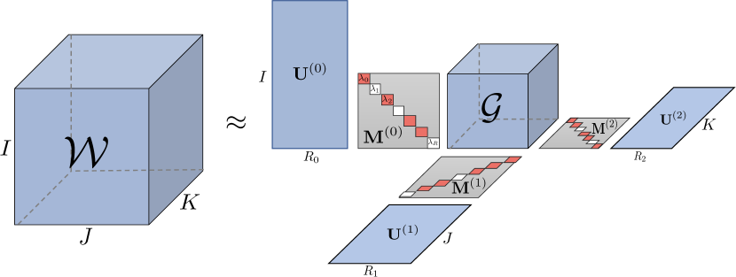
Figure 16: Tensor Dropout on a Tucker decomposition. Visualization of tensor dropout applied to a Tucker decomposition. Several types of randomization can be used. Here, a Bernouilli dropout is represented, applied in the latent subspace of the decomposition, by contracting the core along each mode with a series of (diagonal) Bernouilli sketching matrices, $\mathbf{M}^{(k)}=\operatorname*{diag}({\mathbf{\lambda}^{(k)}})$.

V-E2 Defensive Tensorization

By combining the reparametrization approach described in section V-D5 with tensor dropout, one can drastically improve the robustness of a DCNN to adversarial attacks. When combined with adversarial training, this approach proved successful against a wide range of attacks [151].

V-E3 Tensor-Shield

In addition to the line of research that consists in modifying the weights or activations of the network to increase robustness to adversarial attacks, it is possible to modify the input imagee directly. For instance, Shield [152] uses a JPEG encoding to remove any potential adversarial noise. However, the defensive capacity of this approach is limited. Instead of a JPEG encoding, in [153] tensor decomposition techniques are utilized as a preprocessing step to find a low-rank approximation of images which can significantly discard high-frequency perturbations.

V-F Tensor structures in polynomial networks and attention mechanisms

Notebook: polynomial_neural_network_astroid_generation.ipynb

Apart from CNNs, tensor structures arise in polynomial networks and attention mechanisms, capturing higher-order (e.g., multiplicative) interactions among data or parameters. Here, we provide an overview of how tensor methods are incorporated within such models.

Multiplicative interactions and polynomial function approximation have long been used in the domain of machine learning. Group Method of Data Handling (GMDH) [154] proposes building quadratic polynomials from input elements. The elements in each quadratic polynomial are predetermined, which does not allow the method to capture data-driven correlations among different elements. The method was later extended in higher-order polynomials [155]. Low-order polynomial networks were also used in pi-sigma [156] and sigma-pi-sigma [157]. The pi-sigma network includes a single hidden layer, and the output is the product of all hidden representations with fixed weights equal to $1$. The idea of sigma-pi-sigma is to sum multiple pi-sigma networks. In the context of kernel methods, Factorization Machines [158] and their higher-order extension [159] model both low- and higher-order interactions between variables, using factorized parameters via matrix/tensor decompositions. By employing factorized parameters, such models are able to estimate higher-order interactions even in tasks where data are sparse (e.g., recommender systems), unlike other kernel methods such as SVMs.

More recently, deeper neural networks have been proposed to capture multiplicative interactions [160, 161]. For instance, Highway networks [160] introduce an architecture that enables second-order interactions between the inputs. In [162], the authors augment the original convolution with a multiplicative interaction to increase representational power. In [161], the authors group several such multiplicative interactions as a second-order polynomial and prove that the second-order polynomials extend the class of functions that can be represented with zero error.

Recent empirical [163, 164, 165] and theoretical [161] results indicate that multivariate higher-order polynomials expand the classes of functions that can be approximated with deep neural networks. Approximating a function using a multivariate higher-order polynomial involves learning the multivariate polynomial expansion parameters using input-output training data. Higher-order tensors naturally represent the parameters of such a multivariate polynomial [166], whose dimensionality increases exponentially to the order of the polynomial approximation. This is another instance of the curse of dimensionality that tensor decompositions can mitigate. Moreover, in this setting, choosing different tensor decompositions results in different recursive equations that compose the polynomial function approximation and are hence linked to different neural network architectures.

Particularly, let $\bm{z}\in\mathbb{R}^{d}$ be the input, e.g., the latent noise in a generative model, or an image in a discriminative model, and let $\bm{x}\in\mathbb{R}^{o}$ be the target, e.g., an output image or a class-label. A polynomial expansion of the input $\bm{z}$ can be considered for approximating the target $\bm{x}$. That is, a vector-valued function $\bm{G}(\bm{z}):\mathbb{R}^{d}\to\mathbb{R}^{o}$ expresses the high-order multivariate polynomial expansion:

$$\bm{x}=G(\bm{z})=\sum_{n=1}^{N}\bigg{(}\bm{\mathcal{W}}^{[n]}\prod_{j=2}^{n+1}\times_{j}\bm{z}\bigg{)}+\bm{\beta},$$ (23)

where $\bm{\beta}\in\mathbb{R}^{o}$ and $\big{\{}\bm{\mathcal{W}}^{[n]}\in\mathbb{R}^{o\times\prod_{m=1}^{n}\times_{m}d}\big{\}}_{n=1}^{N}$ are the learnable parameters. The form of (23) can approximate any smooth function (for large $N$). As aforementioned the number of parameters required to accommodate all higher-order interactions of the input increases exponentially with the desired order of the polynomial which is impractical for high-dimensional data. To make this model practical, its parameters can be reduced by making a) low-rank assumptions, and b) sharing factors between the decompositions of each parameter tensor, which accounts to jointly factorize all the parameter tensors $\bm{\mathcal{W}}^{[n]}$. To illustrate this, a certain form of CP decomposition with shared factors among low-rank decompositions of weight tensors [164] is selected. Concretely, the parameter tensor $\bm{\mathcal{W}}^{[n]}$ is factorized using $n$ factor matrices. The first and the last factor matrices (called $\bm{U}_{[{1}]}$ and $\bm{C}$ respectively) are shared across all parameter tensors. Then, depending on the interactions between the layers we want to forge, we can share the corresponding factor matrices. That results (see [164, 169] for detailed derivation) in a simple recursive relationship, that can be expressed as:

$$\bm{x}_{n}=\Big{(}\bm{U}_{[{n}]}^{T}\bm{z}\Big{)}*\bm{x}_{n-1}+\bm{x}_{n-1},$$ (24)

for $n=2,\ldots,N$ with $\bm{x}_{1}=\bm{U}_{[{1}]}^{T}\bm{z}$ and $\bm{x}=\bm{C}\bm{x}_{N}+\bm{\beta}$. The parameters $\bm{C}\in\mathbb{R}^{o\times k},\bm{U}_{[{n}]}\in\mathbb{R}^{d\times k}$ for $n=1,\ldots,N$ are learnable with $k\in\mathbb{N}$ the rank of the CP decomposition.

Each recursive call in (24) expands the approximation order by one. Then, the final output $\bm{x}$ is a polynomial of $N^{th}$ order. The recursive relationship of (24) enables us to implement the polynomial using a hierarchical neural network, where the approximation order defines the depth of the network. A schematic assuming a third-order expansion ($N=3$) is illustrated in Fig. 17. The tensor decomposition selected and the sharing of the factors have a crucial role in the resulting architecture. As aforementioned, by selecting different decompositions, new architectures can emerge [164], while additional constraints can be placed on the structure, e.g., shift invariance by allowing factor matrices to implement convolutions (e.g., via im2col operator or a circulant operator).

Higher-order polynomials can be represented as a product of lower-order polynomials, which have been extensively studied for both univariate and multivariate cases. Berlekamp’s algorithm [170] was one of the first for successfully factoring univariate polynomials over finite fields; the Cantor–Zassenhaus algorithm [171] has since become more popular. Factorizing multivariate polynomials as a linear combination of univariate polynomials has recently been studied using tensor decompositions [172]. The work of [173] demonstrates that the aforementioned factorization of multivariate polynomials is related to the joint CP decomposition.

In deep polynomial networks, instead of using a single polynomial, also products of polynomials can be used [164]. That is, the higher-order multivariate polynomial function is expressed as a product of low-order multivariate polynomials. This approach enforces variable separability in two levels. First, in the parameters of low-order polynomials via tensor decomposition as aforementioned, and second by allowing approximation as a product of simpler functions. The product of polynomials increases the expansion order without increasing the number of layers significantly.

Figure 17: Schematic illustration of the polynomial expansion for third order approximation.

Furthermore, the original attention mechanism [174] is focused on neural machine translation, yet it expresses multiplicative interactions. The idea is to capture long-range dependencies that might exist in a temporal sequence. This was later extended to attention mechanisms for image and video data [175]. Multi-head attention learns different matrices per head; concatenating those matrices, a third-order tensor is obtained. The authors utilize a CP decomposition to both reduce the parameters and reduce the redundancy in the learned matrices [176]. In [177], where the authors extend self-attention to capture not only inter- but also intra-channel correlations by constructing an appropriate tensor such that the variance of spatial-and channel-wise features is regularized.

VI Applications in Computer Vision

In this section, we firstly discuss applications related to extracting multiple latent factors of variation from visual data (Section VI-A). An overview of applications that focus on feature extraction with multilinear subspace learning is presented in Section VI-B, while applications in inverse problems such as denoising and completion are presented in Section VI-C. In Section VI-D, tensor regression applications in visual classification are discussed. Finally, in Section VI-E, some recent applications of tensor-parametrized deep learning architectures are briefly presented

VI-A Multiple factors analysis in computer vision

Notebook: tensorfaces.ipynb

Extracting multiple hidden factors of variation from visual data is a first fundamental step in a large number of computer vision applications. Consider the problem of view- and pose-invariant visual object classification, where one needs to classify visual objects captured across different perspectives and poses. To achieve this, it is required to design or learn data representations that are invariant to view and pose changes, and at the same time, capture discriminant information regarding the object’s category. Structure from motion (which aims to estimate 3D structures from two-dimensional image sequences) is another computer vision task where disentanglement of multiple factors is required. More specifically, one needs to disentangle shape and motion factors and subsequently exploit them in reconstructing 3D visual objects. Face editing [178, 179] and talking faces synthesis [180] are further problems requiring the manipulation of multiple latent variables.

Multiple factors analysis via tensor methods is achieved using two different approaches. The first and historically oldest approach flattens visual data to vectors, which are then arranged into a tensor according to the factors involved in their formation to prepare the data for subsequent analysis. The second, more recent approach assumes a tensor-structured latent space in deep autoencoder-based architectures [181]).

The TensorFaces [182] is probably the most popular method in the first category and has been widely employed to analyze visual data of known sources of variation. For instance PIE [183] and Multi-PIE [184] databases contain a number of people (i.e., multiple identities) captured under different poses and illuminations, displaying a variety of facial expressions. Likewise, the Weizmann face dataset [185] consists of $28$ subjects in $5$ viewpoints, $4$ illuminations, and $3$ expressions. Following the TensorFaces framework, such datasets are represented by a tensor with order equal to the number of sources of variation, and vectorized images are arranged into its fibers according to the labels that describe the sources of variation. The Weizmann dataset, for example, would represented by a $28\times 5\times 4\times 3\times 7943$ tensor $\mathcal{{X}}$, where each image consists of $7943$ pixels. TensorFaces uncover the latent factors of variation by seeking a decompostion of the form:

$$\mathcal{{X}}=\mathcal{{B}}\times_{1}\mathbf{U}_{people}\times_{2}\mathbf{U}_{views}\times_{3}\mathbf{U}_{illumns}\times_{4}\mathbf{U}_{expres}\times_{5}\mathbf{U}_{pixels},$$ (25)

where matrices $\mathbf{U}$ capture different latent factors of variation and $\mathcal{{B}}$ corresponds to multilinear mixing tensor that entangles the factors of variation. Such factor matrices are employed next for extraction of invariant features. Similar analysis has also been done in analysis of motion signatures [186] and gait sequences [187], disentangling pose and body shape [188, 189], 3D head pose estimation [190], face transfer [191], appearance-based tracking [192, 193], structure from motion, and optical flow [194, 195]. A compositional variant of TensorFaces has also been proposed  [196]. TensorFaces and related approaches [197, 196] are supervised learning models and hence suitable for analysis of visual data collected in tightly controlled conditions.

Unsupervised variants of TensorFaces have been proposed in [10, 198],[199] (extending [200] and [201]). Such methods uncover multiple latent factors of variation from vector data samples in an unsupervised setting (i.e., without the presence of labels). It is only assumed that the number of sources of variation is known. More specifically, let $\bm{X}\in\mathbb{R}^{d\times N}$ be a matrix of observations, where each of the $N$ columns represents a vectorized image of $d$ pixels. Each image is assumed to be formed by the entanglement of $M-1$ different, yet unknown sources of variation as:

$$\mathbf{x}_{i}=\mathcal{{B}}\times_{2}\mathbf{u}^{(2)}_{i}\times_{3}\mathbf{a}^{(u)}_{i}\times_{4}\dots\times_{m}\mathbf{u}^{(M)}_{i}.$$ (26)

Each factor $\mathbf{u}_{i}^{(m)}$ accounts for a source of variability in the data, while the multiplicative interactions of these factors through tensor $\mathcal{{B}}\in\mathbb{R}^{d\times K_{2}\times\cdots\times K_{M}}$ emulate the entangled variability giving rise to the rich structure of image $\mathbf{x}_{i}$. For a set of images represented by the observation matrix $\bm{X}$, the above model is written in matrix form as [10, 198]:

$$\mathcal{{X}}=\mathbf{B_{(1)}}(\mathbf{U}^{(2)}\odot\mathbf{U}^{(3)}\cdots\odot\mathbf{U}^{(M)}),$$ (27)

where $\mathbf{B_{(1)}}\mathbb{R}^{d\times K_{2}\cdot K_{3}\cdots K_{M}}$ is the mode-$1$ unfolding of $\bm{\mathcal{B}}$ and $\{\bm{U}^{(m)}\}_{m=2}^{M}\in\mathbb{R}^{K_{m}\times N}$ gathers the variation coefficients for all images across $M-1$ modes of variation. Observe that this model is different from the Tucker decomposition and does not require labels for the data tensor formation, in contrast to TensorFaces. To find the unknown latent factors and the mixing operator, the reconstruction error $\|\mathcal{{X}}-\mathbf{B_{(1)}}(\mathbf{U}^{(2)}\odot\mathbf{U}^{(3)}\cdots\odot\mathbf{U}^{(M)})\|_{F}^{2}$ is minimized. Having found the disentangled modes of variation, they can subsequently be used to drive shape from shading, face editing (expression transfer), and estimation of surface normals [10, 198] and viewpoint and illumination invariant face recognition [199].

In the second family of methods, the multilinear structure is imposed on the latent space of deep autoencoder-based models. More specifically, [178, 179, 202], employ CNN-based encoders to obtain a set of $M-1$ latent vector representations $\{\mathbf{u}_{i}^{(m)}\}_{m=2}^{M}$ for each image using label information. Each factor accounts for a source of variability in the data, while the multiplicative interactions of these factors emulate the entangled variability using (26). The entangled latent variable is fed into a decoder network that reconstructs each image. In this setting, the autoencoder parameters and the tensor $\mathcal{{B}}$ are trained end-to-end. Such models can be used then for image editing (e.g., face editing) via manipulating the latent factors of variation. A similar parameterization of the latent space of conditional deep variational autoencoders has been employed in [203] allowing to generate images formed by combinations of sources of variation that have not been observed in training data.

VI-B Dimensionality reduction via tensor component analysis

Tensor component analysis such as tensor extensions of PCA and LDA (cf. Section IV-D) and decompositions have found a surge of applications in dimensionality reduction and features extraction from tensor-valued visual data. Subsequently, the extracted features are utilized for downstream tasks such as classification, using learning models such as nearest-neighbors, SVMs, or neural networks. In human sensing applications, tensor component analysis methods are applied directly on face or body silhouette images, and the extracted features are used for face recognition, and body/gait analysis [105, 109, 204, 205, 206, 207]. Besides modeling variation on texture, tensor component analysis models, such as the HOSVD, have been used to build statistical shape models in the context of Active Appearance Models (AAM) [208, 209] instead of the linear model typically used [210]. Furthermore, the Tucker decomposition has been used for image compression [211, 212].

In the domain of hyperspectral image analysis, tensor component analysis methods can be used to reduce the statistical redundancy resulting from high interband correlations [213]. For instance, in [214], discriminant features are extracted for classification by applying the tensor discriminative locality alignment (TDLA) method onto a data tensor consisting of hyperspectral image patches.

Variants of tensor networks and decompositions have been further employed for tasks such as tumor and legion detection from visual data [215, 216], showing benefits both in terms of performance and computational cost. Unsupervised coupled matrix-tensor factorization methods have also been proposed towards identifying coherent brain regions across subjects that activate when similar stimuli are provided [217].

VI-C Tensor methods in inverse problems

Inverse problems in imaging span a wide range of tasks, such as image restoration via denoising and completion of missing visual data (imputation). By representing visual as tensors, models addressing inverse problems exploit low-rank tensor decompositions (Section IV-B), or rely on robust variants (Sections IV-C IV-E) to estimate a low-rank tensor which forms a basis from which missing data can be imputed or denoised. Along this line of research, several methods for image and video inpainting and/or denoising have been developed by estimating the low-rank tensor using either nuclear norm-based regularizers, or by assuming an explicit low-rank tensor structure described by decompositions such CP, Tucker, Tensor Ring, or TT decomposition [218, 219, 220, 221, 92, 99, 100, 101, 98]. For the same task, methods based on tensor-structured separable dictionary learning (Section IV-E) have also been proposed [4, 115, 11]. In the context of hyperspectral image analysis, data are corrupted with more complex noise distributions specific to the domain, such as impulse noise and stripings. To denoise, such data, regularized variants of the CP decomposition have been employed [222, 223, 224]. Experimental results indicate increased stability and accuracy compared to methods that do not exploit the tensor structure of the data.

In [225], several extensions of multilinear component analysis methods are presented, emphasizing the discovery of common features shared by multiple data views - such as common and individual feature analysis, with applications in MRI denoising and completion.

VI-D Tensor regression for visual classification

Low-rank tensorregression models are well-suited for classification of large-scale visual data, such as face and body images and videos, as well as hyperspectral and medical images. In [5], low-rank tensor regression models with automatic rank selection are applied on problems such as face classification and pose estimation, while in [123], a multilinear multitask learning framework is used for pain estimation from videos. Low-rank quantile tensor regression is also utilized in [128] and applied for crowd counting on image datasets. In [226], tensor logistic regression is employed towards land-cover classification from hyperspectral data. It effectively reduces the number of parameters compared to methods that treat hyperspectral images as vectors from $C\prod_{i=1}^{N}{I_{i}}$ to $C\sum_{i=1}^{N}I_{i}$, where $C$ indicates the number of classes and $N$ is the order of the tensor describing the data. Classification of fMRI images may relate to several target variables, for example, detecting and identifying disease and brain damage and human brain activity that can be associated with stimuli context. A variety of tensor methods has been used to this end, such as tensor extensions to SVM [227] and regularized low-rank tensor regression models [119, 122, 120].

VI-E Deep networks parametrization using tensor decomposition

The vast majority of the deep learning models discussed in Section V have been introduced in the context of image classification, and their effectiveness have been studied in large-scale standard benchmark datasets such as ImageNet. Neural network compression using CP decomposition has also been applied on land-cover classification  [226]. Furthermore, CNNs with tensor regression layers have also been used for various applications such as affect estimation from faces [228, 27]. Randomized TRL has been employed in age prediction from MRI scans [33], significantly improving the results with respect to state-of-the-art algorithms.

Mobilenet V1 [229] and Mobilenet V2 [230] are seminal light-weight architectures allowing mobile and embedded vision applications. Interestingly, these architectures can be interpreted as special cases of Kruskal and Tucker convolutions described in Section V-D. The interested reader is referred to [27, 141] for details.

Parametrizing one or several layers with a low-rank tensor factorization has several advantages, namely robustness to noise, regularizing effect, computational speedups, and reduction in the number of parameters. Another advantage is conceptual: the structure induced by the factorization can be used to adapt a model to different domains or efficiently share information between tasks. For instance, when applying a Tucker decomposition to a tensor, we obtain a latent subspace represented by the core tensor. We can project to and from that space using the factors of the decomposition, which are typically projection matrices. This enables various applications, including cross-task and cross-domain incremental learning, typically by allowing weight sharing through joint factorization. [28] propose weight sharing in multitask learning and [29] propose sharing residual units. Most recently, [30] proposed to learn a task agnostic core, which is shared between tasks and domains. This shared subspace can be specialized to the new task or domain by learning a new set of task-specific projection matrices.

VII Challenges and Practitioner’s Guide

Tensor methods are handy tools for learning from multi-dimensional data and a convenient framework for infusing more structure in deep neural networks, leveraging redundancy to obtain more compact models, and increasing robustness. However, some challenges may currently prevent their wider adoption, especially in the context of deep learning. This section highlights such significant challenges and guides practitioners on how to tackle them in practice.

Rank selection. Most tensor methods discussed in this paper require knowledge or estimation of the rank of the decomposition. However, determining the rank of a tensor is, in general, NP-hard [78, 79] and usually heuristics are employed in practice. While the choice of exact rank within a deep framework is less crucial as all the parameters are trained end-to-end jointly; rank selection remains a significant challenge.

In practice, one can start with selecting a rank such that $90\%$ of the parameters are preserved and incrementally reduce the rank, e.g., through multi-stage compression [145]. When starting from a pre-trained networks, it is also possible to approximate the rank by applying Bayesian matrix factorization [231] to the unfolding of the weight tensor to get an approximation of the rank [140, 145]. Alternatively, a Lasso-type penalty can be added to the loss function to automatically set some of the components to zero [27].

Which decomposition to use? Another significant open question in tensor methods is the choice of decomposition. While there are heuristics developed through intuition and experimental work, there is no principled way to choose the most appropriate decomposition.

In practice, as a rule of thumb, the Tucker decomposition is well suited for subspace learning as it allows to project to and from the latent subspace represented by its core. The CP decomposition is well suited for learning interpretable latent factors; however, it is less suited for decomposing tensors which have some very large modes and some smaller ones, since the same rank is used for all dimensions. The Tensor-Train decomposition is best when the goal is to achieve very high compression ratios, as it disentangles the dimensions. In fact, it may be desirable to jointly model dimensions if we want to preserve the correlations between them [21].

Similar intuition applies to the choice of tensor decomposition in the context of deep learning, albeit with some additional considerations. A CP factorization can be seen as a MobileNet-v2 block, where the rank is equal to the product of the expansion factor with the number of input channels. This means that for achieving speedups, one should choose the rank accordingly, e.g., to be a power of $2$. CP is a beneficial choice when combined with transduction to train, e.g., on a static domain such as images, and then generalize to videos [27] during inference. A Tucker convolution gives more flexibility by allowing each mode to have a different rank, but the rank chosen along the input and output channels should also be chosen with speed in mind. For efficient learning of convolutional LSTMs in higher-orders, convolutional tensor-train decompositions have proven successful [232].

As we established in Section V, there is an equivalence between choosing the tensor decomposition applied to convolutional kernels and choosing an efficient convolutional block, and an equivalence between finding the decomposition’s rank and finding the block’s parameters. Clearly, choosing the appropriate tensor decomposition and its rank depends on the tensor structure, and therefore the two problems are intertwined. However, there is currently a lack of theory to guide optimal choices and enable efficient search over model architectures. Furthermore, auto-tensorization is of particular interest. In other words, given a (pre-trained) existing network architecture, an interesting question is how to automatically choose the decomposition and its rank to approximate the network in a compressed form optimally.

Training tensorized deep neural networks. Training tensorized deep neural networks remains a challenging task due to mainly numerical issues. For instance, composing several tensor contractions can lead to instability, with the gradient vanishing or exploding. This is particularly true when using lower precisions (e.g., int8) motivating the need for principled ways to initialize the factors of tensor decompositions, and the need for better normalization methods that can take into account the structure.

In practice, using full precision (i.e., ‘float64’) can alleviate most of such numerical issues. However, in order to speed up learning and inference, modern deep learning systems often rely on reduced precision, e.g., float32, or even adopt quantization of the deep models to int16, int8, or just binary, which in turn can cause numerical stability issues. To enable robust and stable learning in such settings, one can use automatic mixed-precision software tools (available for instance through NVIDIA’s Amp). Automatic mixed-precision relies on two parts: using reduced precision when this can be done without affecting performance and automatic loss scaling to preserve small gradient values. On the hardware side, better handling of mathematical operations allows for striking a balance between speed and precision, for example by using tensor floats. Tensor floats on 32 bits (TF32), for instance, use the same mantissa as half-precision (Float16) but still use an 8-bit exponent to support a larger numerical range. Alternatively, it is possible to perform the calculations in log-space. While such an approach improves numerical stability, it limits the range to positive values only.

Finally, it should be noted that a careful initialization of the factors of the decomposition is crucial to ensure that the values of the reconstruction are in the expected range. It is well known that deep convolutional neural networks need to be carefully initialized, e.g., using the He [233] or Glorot [234] initialization. These typically use a Gaussian distribution with a zero-mean and small variance. It is possible to perform variance analysis and initialize the factors directly, so the reconstruction has zero-mean and a given variance.

References

- [1] S. Montangero, S. Montangero, and Evenson, Introduction to Tensor Network Methods. Springer, 2018.
- [2] J. M. Landsberg, “Tensors: geometry and applications,” Representation theory, vol. 381, no. 402, p. 3, 2012.
- [3] H. Lu, K. N. Plataniotis, and A. Venetsanopoulos, Multilinear Subspace Learning: Dimensionality Reduction of Multidimensional Data, 1st ed. Chapman & Hall/CRC, 2013.
- [4] M. Bahri, Y. Panagakis, and S. Zafeiriou, “Robust Kronecker component analysis,” IEEE Trans. Pattern Anal. Mach. Intell., vol. 41, pp. 2365–2379, 2019.
- [5] W. Guo, I. Kotsia, and I. Patras, “Tensor learning for regression,” IEEE Trans. Image Process., vol. 21, no. 2, pp. 816–827, Feb 2012.
- [6] A. Anandkumar, R. Ge, D. Hsu, S. M. Kakade, and M. Telgarsky, “Tensor decompositions for learning latent variable models,” J. Mach. Learn. Res., vol. 15, pp. 2773–2832, 2014.
- [7] R. Bellman, Adaptive Control Processes. Princeton University Press, 1961.
- [8] H. Lu, K. N. Plataniotis, and A. N. Venetsanopoulos, “A survey of multilinear subspace learning for tensor data,” Pattern Recognit., vol. 44, no. 7, pp. 1540–1551, 2011.
- [9] A. Shashua and T. Hazan, “Non-negative tensor factorization with applications to statistics and computer vision,” in Proc. Int. Conf. Mach. Learn. (ICML), 2005, pp. 792–799.
- [10] M. Wang, Y. Panagakis, P. Snape, and S. P. Zafeiriou, “Disentangling the modes of variation in unlabelled data,” IEEE Trans. Pattern Anal. Mach. Intell., vol. 40, no. 11, pp. 2682–2695, 2018.
- [11] S. Hawe, M. Seibert, and M. Kleinsteuber, “Separable dictionary learning,” Proc. IEEE Conf. Comput. Vis. Pattern Recognit. (CVPR), Jun 2013.
- [12] Y. LeCun, Y. Bengio, and G. Hinton, “Deep learning,” Nature, vol. 521, no. 7553, p. 436–444, May 2015.
- [13] Y. LeCun, Y. Bengio et al., “Convolutional networks for images, speech, and time series,” The Handbook of Brain Theory and Neural Netw., vol. 3361, no. 10, p. 1995, 1995.
- [14] A. Krizhevsky, I. Sutskever, and G. E. Hinton, “ImageNet classification with deep convolutional neural networks,” in Advances in Neural Inf. Process. Syst. (NeurIPS), 2012, pp. 1097–1105.
- [15] K. He, X. Zhang, S. Ren, and J. Sun, “Deep residual learning for image recognition,” in Proc. IEEE Conf. Comput. Vis. Pattern Recognit. (CVPR), 2016.
- [16] Y. LeCun, L. Bottou, Y. Bengio, and P. Haffner, “Gradient-based learning applied to document recognition,” Proc. IEEE, vol. 86, no. 11, pp. 2278–2324, 1998.
- [17] S. S. Du and J. D. Lee, “On the power of over-parametrization in neural networks with quadratic activation,” in Proc. Int. Conf. Mach. Learn. (ICML), 2018.
- [18] M. Soltanolkotabi, A. Javanmard, and J. D. Lee, “Theoretical insights into the optimization landscape of over-parameterized shallow neural networks,” IEEE Trans. Inf. Theory, 2018.
- [19] R. Caruana, S. Lawrence, and L. Giles, “Overfitting in neural nets: Backpropagation, conjugate gradient, and early stopping,” in Advances in Neural Inf. Process. Syst. (NeurIPS), 2001.
- [20] H. Mhaskar, Q. Liao, and T. Poggio, “Learning functions: when is deep better than shallow,” arXiv preprint arXiv:1603.00988, 2016.
- [21] A. Novikov, D. Podoprikhin, A. Osokin, and D. Vetrov, “Tensorizing neural networks,” in Advances in Neural Inf. Process. Syst. (NeurIPS), 2015, pp. 442–450.
- [22] V. Lebedev, Y. Ganin, M. Rakhuba, I. V. Oseledets, and V. S. Lempitsky, “Speeding-up convolutional neural networks using fine-tuned CP-decomposition,” in Proc. Int. Conf. Learn. Representations (ICLR), 2015.
- [23] M. Astrid and S. Lee, “CP-decomposition with tensor power method for convolutional neural networks compression,” CoRR, vol. abs/1701.07148, 2017.
- [24] J. Kossaifi, A. Khanna, Z. Lipton, T. Furlanello, and A. Anandkumar, “Tensor contraction layers for parsimonious deep nets,” in Proc. IEEE Conf. Comput. Vis. Pattern Recognit. (CVPR), 2017, pp. 1940–1946.
- [25] J. Kossaifi, Z. C. Lipton, A. Kolbeinsson, A. Khanna, T. Furlanello, and A. Anandkumar, “Tensor regression networks,” J. Mach. Learn. Res., vol. 21, no. 123, pp. 1–21, 2020.
- [26] J. Kossaifi, A. Bulat, G. Tzimiropoulos, and M. Pantic, “T-Net: Parametrizing fully convolutional nets with a single high-order tensor,” in Proc. IEEE Conf. Comput. Vis. Pattern Recognit. (CVPR), 2019, pp. 7814–7823.
- [27] J. Kossaifi, A. Toisoul, A. Bulat, Y. Panagakis, T. M. Hospedales, and M. Pantic, “Factorized higher-order CNNs with an application to spatio-temporal emotion estimation,” in Proc. IEEE Conf. Comput. Vis. Pattern Recognit. (CVPR), 2020, pp. 6060–6069.
- [28] Y. Yang and T. M. Hospedales, “Deep multi-task representation learning: A tensor factorisation approach,” in Proc. Int. Conf. Learn. Representations (ICLR), 2017.
- [29] Y. Chen, X. Jin, B. Kang, J. Feng, and S. Yan, “Sharing residual units through collective tensor factorization to improve deep neural networks,” in Proc. of the Twenty-Seventh Int. Joint Conf. on Artif. Intell., IJCAI-18. Int. Joint Conf. on Artif. Intell. Org., 7 2018, pp. 635–641.
- [30] A. Bulat, J. Kossaifi, G. Tzimiropoulos, and M. Pantic, “Incremental multi-domain learning with network latent tensor factorization,” Proc. AAAI Conf. Artif. Intell. (AAAI), 2020.
- [31] I. Goodfellow, J. Pouget-Abadie, M. Mirza, B. Xu, D. Warde-Farley, S. Ozair, A. Courville, and Y. Bengio, “Generative adversarial nets,” in Advances in Neural Inf. Process. Syst. (NeurIPS), 2014.
- [32] A. Madry, A. Makelov, L. Schmidt, D. Tsipras, and A. Vladu, “Towards deep learning models resistant to adversarial attacks,” in Proc. Int. Conf. Learn. Representations (ICLR), 2018.
- [33] A. Kolbeinsson, J. Kossaifi, Y. Panagakis, A. Anandkumar, I. Tzoulaki, and P. Matthews, “Tensor dropout for robust learning,” CoRR, vol. abs/1902.10758, 2020.
- [34] T. G. Kolda and B. W. Bader, “Tensor decompositions and applications,” SIAM Rev., vol. 51, no. 3, pp. 455–500, 2009.
- [35] P. Comon, “Tensors: a brief introduction,” IEEE Signal Process. Mag., vol. 31, pp. 44–53, 05 2014.
- [36] N. D. Sidiropoulos, L. De Lathauwer, X. Fu, K. Huang, E. E. Papalexakis, and C. Faloutsos, “Tensor decomposition for signal processing and machine learning,” IEEE Trans. Signal Process., vol. 65, no. 13, pp. 3551–3582, 2017.
- [37] A. Cichocki, D. Mandic, L. De Lathauwer, G. Zhou, Q. Zhao, C. Caiafa, and H. A. PHAN, “Tensor decompositions for signal processing applications: From two-way to multiway component analysis,” IEEE Signal Process. Mag., vol. 32, no. 2, pp. 145–163, 2015.
- [38] E. E. Papalexakis, C. Faloutsos, and N. D. Sidiropoulos, “Tensors for data mining and data fusion: Models, applications, and scalable algorithms,” ACM Trans. Intell. Syst. and Technol. (TIST), vol. 8, no. 2, pp. 1–44, 2016.
- [39] A. Smilde, R. Bro, and P. Geladi, “Multi-way analysis with applications in the chemical sciences,” J. Chemometrics, vol. 19, no. 2, pp. 119–120, 2005.
- [40] E. Acar and B. Yener, “Unsupervised multiway data analysis: A literature survey,” IEEE Trans. Know. Data Eng., vol. 21, no. 1, pp. 6–20, 2008.
- [41] A. Cichocki, R. Zdunek, A. H. Phan, and S.-i. Amari, Nonnegative matrix and tensor factorizations: applications to exploratory multi-way data analysis and blind source separation. John Wiley & Sons, 2009.
- [42] M. Janzamin, R. Ge, J. Kossaifi, A. Anandkumar et al., “Spectral learning on matrices and tensors,” Found. and Trends® in Mach. Learn., vol. 12, no. 5-6, pp. 393–536, 2019.
- [43] H. A. Kiers, “Towards a standardized notation and terminology in multiway analysis,” J. Chemometrics, vol. 14, no. 3, pp. 105–122, 2000.
- [44] J. Kossaifi, Y. Panagakis, A. Anandkumar, and M. Pantic, “Tensorly: Tensor learning in python,” J. Mach. Learn. Res., vol. 20, no. 26, pp. 1–6, 2019.
- [45] A. Paszke, S. Gross, S. Chintala, G. Chanan, E. Yang, Z. DeVito, Z. Lin, A. Desmaison, L. Antiga, and A. Lerer, “Automatic differentiation in PyTorch,” in Advances in Neural Inf. Process. Syst. (NeurIPS), 2017.
- [46] D. L. Donoho, “For most large underdetermined systems of linear equations the minimal L1-norm solution is also the sparsest solution,” Commun. on Pure and Appl. Math., vol. 59, no. 6, pp. 797–829, 2006.
- [47] F. Maryam, “Matrix rank minimization with applications,” Ph.D. dissertation, Stanford University, 2002.
- [48] R. Raina, A. Madhavan, and A. Y. Ng, “Large-scale deep unsupervised learning using graphics processors,” in Proc. Int. Conf. Mach. Learn. (ICML). New York, NY, USA: Assoc. for Comput. Machinery, 2009, p. 873–880.
- [49] D. C. Cireşan, U. Meier, J. Masci, L. M. Gambardella, and J. Schmidhuber, “Flexible, high performance convolutional neural networks for image classification,” in Proc. Twenty-Second Int. Joint Conf. Artif. Intell., ser. IJCAI’11. AAAI Press, 2011, p. 1237–1242.
- [50] Y. Shi, U. N. Niranjan, A. Anandkumar, and C. Cecka, “Tensor contractions with extended BLAS kernels on CPU and GPU,” in IEEE Int. Conf. High Perform. Comput. (HiPC), Dec 2016, pp. 193–202.
- [51] P. Springer and M. Hoehnerbach. (2019) cuTENSOR: A high-performance CUDA library for tensor primitives. [Online]. Available: https://docs.nvidia.com/cuda/cutensor/index.html
- [52] M. Abadi, A. Agarwal, P. Barham, E. Brevdo, Z. Chen, C. Citro, G. S. Corrado, A. Davis, J. Dean, M. Devin, S. Ghemawat, I. Goodfellow, A. Harp, G. Irving, M. Isard, Y. Jia, R. Jozefowicz, L. Kaiser, M. Kudlur, J. Levenberg, D. Mané, R. Monga, S. Moore, D. Murray, C. Olah, M. Schuster, J. Shlens, B. Steiner, I. Sutskever, K. Talwar, P. Tucker, V. Vanhoucke, V. Vasudevan, F. Viégas, O. Vinyals, P. Warden, M. Wattenberg, M. Wicke, Y. Yu, and X. Zheng, “TensorFlow: Large-scale machine learning on heterogeneous systems,” 2015, software available from tensorflow.org.
- [53] T. Chen, M. Li, Y. Li, M. Lin, N. Wang, M. Wang, T. Xiao, B. Xu, C. Zhang, and Z. Zhang, “MXNet: A flexible and efficient machine learning library for heterogeneous distributed systems,” CoRR, vol. abs/1512.01274, 2015.
- [54] N. P. Jouppi, C. Young, N. Patil, D. Patterson, G. Agrawal, R. Bajwa, S. Bates, S. Bhatia, N. Boden, A. Borchers et al., “In-datacenter performance analysis of a tensor processing unit,” in Proc. Annu. Int. Symp. Comput. Architecture, 2017, pp. 1–12.
- [55] (2020) Tensorly-torch. [Online]. Available: https://github.com/tensorly/torch
- [56] A. Novikov, P. Izmailov, V. Khrulkov, M. Figurnov, and I. Oseledets, “Tensor train decomposition on tensorflow (t3f),” J. Mach. Learn. Res., vol. 21, no. 30, pp. 1–7, 2020.
- [57] R. Ballester-Ripoll. (2018) tntorch – tensor network learning with pytorch. [Online]. Available: https://github.com/rballester/tntorch
- [58] (2019) Tensor network. [Online]. Available: https://github.com/google/TensorNetwork
- [59] M. Nickel. (2007) scikit-tensor. [Online]. Available: https://github.com/mnick/scikit-tensor/
- [60] B. W. Bader and T. G. Kolda, “MATLAB tensor toolbox version 2.6,” February 2015. [Online]. Available: http://www.sandia.gov/~tgkolda/TensorToolbox/
- [61] N. Vervliet, O. Debals, L. Sorber, M. Van Barel, and L. De Lathauwer, “Tensorlab 3.0,” Mar. 2016. [Online]. Available: https://www.tensorlab.net
- [62] M. Fishman, S. White, and E. M. Stoudenmire, “The itensor software library for tensor network calculations,” ArXiv, vol. abs/2007.14822, 2020.
- [63] C. Choy, J. Gwak, and S. Savarese, “4D spatio-temporal convnets: Minkowski convolutional neural networks,” in Proc. IEEE Conf. Comput. Vis. Pattern Recognit. (CVPR), 2019, pp. 3075–3084.
- [64] F. De la Torre, “A least-squares framework for component analysis,” IEEE Trans. Pattern Anal. Mach. Intell., vol. 34, no. 6, pp. 1041–1055, 2012.
- [65] Z. Zhang, Y. Xu, J. Yang, X. Li, and D. Zhang, “A survey of sparse representation: Algorithms and applications,” IEEE Access, vol. 3, p. 490–530, 2015.
- [66] J. Mairal, F. Bach, J. Ponce, and G. Sapiro, “Online learning for matrix factorization and sparse coding,” J. Mach. Learn. Res., vol. 11, p. 19–60, Mar. 2010.
- [67] F. L. Hitchcock, “The expression of a tensor or a polyadic as a sum of products,” J. of Math. and Phys., vol. 6, no. 1-4, pp. 164–189, 1927.
- [68] J. D. Carroll and J.-J. Chang, “Analysis of individual differences in multidimensional scaling via an n-way generalization of “Eckart-Young” decomposition,” Psychometrika, vol. 35, pp. 283–319, 1970.
- [69] R. A. Harshman, “Foundations of the PARAFAC procedure: Models and conditions for an ”explanatory” multi-modal factor analysis,” UCLA Working Papers in Phonetics, vol. 16, pp. 1–84, 1970.
- [70] K. P. F.R.S., “LIII. on lines and planes of closest fit to systems of points in space,” The London, Edinburgh, and Dublin Philos. Mag. and J. of Sci., vol. 2, no. 11, pp. 559–572, 1901.
- [71] H. Hotelling, “Analysis of a complex of statistical variables into principal components.” J. Educ. Psychol., vol. 24, no. 6, p. 417–441, 1933.
- [72] A. Hyvärinen and E. Oja, “Independent component analysis: algorithms and applications,” Neural Netw., vol. 13, no. 4, pp. 411 – 430, 2000.
- [73] D. Lee and H. Seung, “Learning the parts of objects by non-negative matrix factorization,” Nature, vol. 401, pp. 788–91, 11 1999.
- [74] S. Yan, D. Xu, B. Zhang, H. Zhang, Q. Yang, and S. Lin, “Graph embedding and extensions: A general framework for dimensionality reduction,” IEEE Trans. Pattern Anal. Mach. Intell., vol. 29, no. 1, pp. 40–51, 2007.
- [75] E. J. Candès, X. Li, Y. Ma, and J. Wright, “Robust principal component analysis?” J. ACM, vol. 58, no. 3, Jun. 2011.
- [76] Z. Zhang and D. Tao, “Slow feature analysis for human action recognition,” IEEE Trans. Pattern Anal. Mach. Intell., vol. 34, no. 3, pp. 436–450, 2012.
- [77] A. Mensch, J. Mairal, B. Thirion, and G. Varoquaux, “Dictionary learning for massive matrix factorization,” in Proc. Int. Conf. Mach. Learn. (ICML), ser. ICML’16. JMLR.org, 2016, p. 1737–1746.
- [78] J. Håstad, “Tensor rank is NP-complete,” J. Algorithms (Print), vol. 11, no. 4, pp. 644–654, 1990.
- [79] C. J. Hillar and L.-H. Lim, “Most tensor problems are NP-hard,” J. ACM, vol. 60, no. 6, Nov. 2013.
- [80] Q. Zhao, L. Zhang, and A. Cichocki, “Bayesian CP factorization of incomplete tensors with automatic rank determination,” IEEE Trans. Pattern Anal. Mach. Intell., vol. 37, no. 9, pp. 1751–1763, 2015.
- [81] P. Rai, Y. Wang, S. Guo, G. Chen, D. Dunson, and L. Carin, “Scalable bayesian low-rank decomposition of incomplete multiway tensors,” in Proc. Int. Conf. Mach. Learn. (ICML), vol. 32, no. 2. Bejing, China: PMLR, 22–24 Jun 2014, pp. 1800–1808.
- [82] M. Zhou, Y. Liu, Z. Long, L. Chen, and C. Zhu, “Tensor rank learning in CP decomposition via convolutional neural network,” Signal Process.: Image Commun., vol. 73, pp. 12 – 21, 2019.
- [83] L. R. Tucker, “Some mathematical notes on three-mode factor analysis,” Psychometrika, vol. 31, pp. 279–311, 1966.
- [84] L. De Lathauwer, B. De Moor, and J. Vandewalle, “A multilinear singular value decomposition,” SIAM J. Matrix Anal. and Appl., vol. 21, no. 4, pp. 1253–1278, 2000.
- [85] M. J. Mohlenkamp, “Musings on multilinear fitting,” Linear Algebra and its Appl., vol. 438, no. 2, pp. 834 – 852, 2013, tensors and Multilinear Algebra.
- [86] I. V. Oseledets, “Tensor-train decomposition,” SIAM J. Sci. Comput., vol. 33, no. 5, pp. 2295–2317, Sep. 2011.
- [87] S. Rommer and S. Östlund, “Class of ansatz wave functions for one-dimensional spin systems and their relation to the density matrix renormalization group,” Phys. Rev. B, vol. 55, pp. 2164–2181, Jan 1997.
- [88] M. Espig, K. K. Naraparaju, and J. Schneider, “A note on tensor chain approximation,” Comput. and Visualization in Sci., vol. 15, no. 6, pp. 331–344, Dec. 2012.
- [89] Q. Zhao, G. Zhou, S. Xie, L. Zhang, and A. Cichocki, “Tensor ring decomposition,” CoRR, vol. abs/1606.05535, 2016.
- [90] P. Huber, “Robust statistics (pp. 1248-1251),” Springer Berlin Heidelberg. Rehabilitation Psychology, vol. 46, pp. 382–399, 2011.
- [91] S. Gandy, B. Recht, and I. Yamada, “Tensor completion and low-n-rank tensor recovery via convex optimization,” Inverse Problems, vol. 27, no. 2, p. 025010, 2011.
- [92] J. Liu, P. Musialski, P. Wonka, and J. Ye, “Tensor completion for estimating missing values in visual data,” IEEE Trans. Pattern Anal. Mach. Intell., vol. 35, no. 1, pp. 208–220, 2012.
- [93] L. Yang, Z.-H. Huang, and X. Shi, “A fixed point iterative method for low n-rank tensor pursuit,” IEEE Signal Process. Lett., vol. 61, no. 11, pp. 2952–2962, 2013.
- [94] D. Goldfarb and Z. T. Qin, “Robust low-rank tensor recovery: Models and algorithms,” SIAM J. Matrix Anal. and Appl., vol. 35, no. 1, pp. 225–253, 2014.
- [95] L. Vandenberghe and S. Boyd, “Semidefinite programming,” SIAM Rev., vol. 38, no. 1, pp. 49–95, 1996.
- [96] B. K. Natarajan, “Sparse approximate solutions to linear systems,” SIAM J. Comput., vol. 24, no. 2, pp. 227–234, 1995.
- [97] Y. Li, J. Yan, Z. Yue, and J. Yang, “Optimum subspace learning and error correction for tensors,” in Proc. Eur. Conf. Comput. Vis. (ECCV), 09 2010, pp. 790–803.
- [98] B. Huang, C. Mu, D. Goldfarb, and J. Wright, “Provable models for robust low-rank tensor completion,” Pacific J. Optim., vol. 11, pp. 339–364, 04 2015.
- [99] W. Hu, D. Tao, W. Zhang, Y. Xie, and Y. Yang, “A new low-rank tensor model for video completion,” ArXiv, vol. abs/1509.02027, 2015.
- [100] S. Gandy, B. Recht, and I. Yamada, “Tensor completion and low-n-rank tensor recovery via convex optimization,” Inverse Problems, vol. 27, no. 2, p. 025010, Jan 2011.
- [101] Y. Liu, F. Shang, W. Fan, J. Cheng, and H. Cheng, “Generalized higher-order orthogonal iteration for tensor decomposition and completion,” in Advances in Neural Inf. Process. Syst. (NeurIPS), 2014, pp. 1763–1771.
- [102] D. G. Chachlakis, A. Prater-Bennette, and P. P. Markopoulos, “L1-norm Tucker tensor decomposition,” IEEE Access, vol. 7, pp. 178 454–178 465, 2019.
- [103] D. Chachlakis, A. Prater-Bennette, and P. Markopoulos, “L1-norm higher-order orthogonal iterations for robust tensor analysis,” in IEEE Int. Conf. Acoustics, Speech, Signal Process. (ICASSP), 2020, pp. 4826–4830.
- [104] D. P. Bertsekas, Constrained Optimization and Lagrange Multiplier Methods (Optimization and Neural Computation Series), 1st ed. Athena Scientific, 1996.
- [105] H. Lu, K. N. Plataniotis, and A. N. Venetsanopoulos, “MPCA: Multilinear principal component analysis of tensor objects,” IEEE Trans. Neural Netw., vol. 19, no. 1, pp. 18–39, 2008.
- [106] Y. Panagakis, C. Kotropoulos, and G. Arce, “Music genre classification using locality preserving non-negative tensor factorization and sparse representations.” in Proc. Int. Soc. Music Information Retrieval. (ISMIR), 01 2009, pp. 249–254.
- [107] Y. Panagakis, C. Kotropoulos, and G. R. Arce, “Non-negative multilinear principal component analysis of auditory temporal modulations for music genre classification,” IEEE Trans. Audio Speech Lang. Process., vol. 18, no. 3, pp. 576–588, 2010.
- [108] S. Yan, D. Xu, Q. Yang, L. Zhang, X. Tang, and H.-J. Zhang, “Multilinear discriminant analysis for face recognition,” IEEE Trans. Image Process., vol. 16, no. 1, pp. 212–220, 2006.
- [109] D. Tao, X. Li, X. Wu, and S. J. Maybank, “General tensor discriminant analysis and gabor features for gait recognition,” IEEE Trans. Pattern Anal. Mach. Intell., vol. 29, no. 10, pp. 1700–1715, 2007.
- [110] Q. Li and D. Schonfeld, “Multilinear discriminant analysis for higher-order tensor data classification,” IEEE Trans. Pattern Anal. Mach. Intell., vol. 36, no. 12, pp. 2524–2537, 2014.
- [111] S. Hsieh, C. Lu, and S. Pei, “2D sparse dictionary learning via tensor decomposition,” in 2014 IEEE Global Conf. Signal Inf. Process. (GlobalSIP), 2014, pp. 492–496.
- [112] Y. Fang, B. Huang, and J. Wu, “2D sparse signal recovery via 2D orthogonal matching pursuit,” Sci. China Inf. Sci., vol. 55, 01 2011.
- [113] Z. Shakeri, W. U. Bajwa, and A. D. Sarwate, “Minimax lower bounds for Kronecker-structured dictionary learning,” 2016 IEEE Int. Symp. Inf. Theory (ISIT), Jul 2016.
- [114] Z. Shakeri, W. U. Bajwa, and A. D. Sarwate, “Minimax lower bounds on dictionary learning for tensor data,” IEEE Trans. Inf. Theory, vol. 64, no. 4, pp. 2706–2726, 2018.
- [115] M. Bahri, Y. Panagakis, and S. Zafeiriou, “Robust Kronecker-decomposable component analysis for low-rank modeling,” in Proc. IEEE Int. Conf. Comput. Vis. (ICCV), 2017, pp. 3372–3381.
- [116] B. Haeffele, E. Young, and R. Vidal, “Structured low-rank matrix factorization: Optimality, algorithm, and applications to image processing,” Proc. Int. Conf. Mach. Learn. (ICML), vol. 5, pp. 4108–4117, 01 2014.
- [117] B. D. Haeffele and R. Vidal, “Global optimality in tensor factorization, deep learning, and beyond,” ArXiv, vol. abs/1506.07540, 2015.
- [118] G. Rabusseau and H. Kadri, “Low-rank regression with tensor responses,” in Advances in Neural Inf. Process. Syst. (NeurIPS), D. D. Lee, M. Sugiyama, U. V. Luxburg, I. Guyon, and R. Garnett, Eds. Curran Associates, Inc., 2016, pp. 1867–1875.
- [119] H. Zhou, L. Li, and H. Zhu, “Tensor regression with applications in neuroimaging data analysis,” J. Amer. Statist. Assoc., vol. 108, no. 502, pp. 540–552, 2013.
- [120] N. Batmanghelich, A. Dong, B. Taskar, and C. Davatzikos, “Regularized tensor factorization for multi-modality medical image classification,” in Int. Conf. Medical Image Comput. and Comput.-Assisted Intervention. Springer, 2011, pp. 17–24.
- [121] R. Yu and Y. Liu, “Learning from multiway data: Simple and efficient tensor regression,” in Proc. Int. Conf. Mach. Learn. (ICML), vol. 48, 20–22 Jun 2016, pp. 373–381.
- [122] X. Song and H. Lu, “Multilinear regression for embedded feature selection with application to fMRI analysis,” in Proc. AAAI Conf. Artif. Intell. (AAAI), 2017.
- [123] B. Romera-paredes, H. Aung, N. Bianchi-berthouze, and M. Pontil, “Multilinear multitask learning,” in Proc. Int. Conf. Mach. Learn. (ICML), S. Dasgupta and D. Mcallester, Eds., vol. 28, no. 3. JMLR Workshop and Conf. Proc., May 2013, pp. 1444–1452.
- [124] X. Li, D. Xu, H. Zhou, and L. Li, “Tucker tensor regression and neuroimaging analysis,” Statist. in Biosci., vol. 10, no. 3, pp. 520–545, Dec. 2018.
- [125] Q. Zhao, C. F. Caiafa, D. P. Mandic, L. Zhang, T. Ball, A. Schulze-bonhage, and A. S. Cichocki, “Multilinear subspace regression: An orthogonal tensor decomposition approach,” in Advances in Neural Inf. Process. Syst. (NeurIPS), 2011, pp. 1269–1277.
- [126] Q. Zhao, C. F. Caiafa, D. P. Mandic, Z. C. Chao, Y. Nagasaka, N. Fujii, L. Zhang, and A. Cichocki, “Higher-order partial least squares (HOPLS): A generalized multi-linear regression method,” CoRR, vol. abs/1207.1230, 2012.
- [127] J. Wu and M. M. Trivedi, “A regression model in TensorPCA subspace for face image super-resolution reconstruction,” in Proc. 18th Int. Conf. on Pattern Recognit. (ICPR), vol. 3. IEEE Comput. Soc., 2006, pp. 627–630.
- [128] W. Lu, Z. Zhu, and H. Lian, “High-dimensional quantile tensor regression,” J. Mach. Learn. Res., vol. 21, no. 250, pp. 1–31, 2020.
- [129] N. Cohen and A. Shashua, “Convolutional rectifier networks as generalized tensor decompositions,” in Proc. Int. Conf. Mach. Learn. (ICML), 2016, pp. 955–963.
- [130] Y. Levine, D. Yakira, N. Cohen, and A. Shashua, “Deep learning and quantum entanglement: Fundamental connections with implications to network design,” in Proc. Int. Conf. Learn. Representations (ICLR), 2018.
- [131] Q. Zhao, M. Sugiyama, L. Yuan, and A. Cichocki, “Learning efficient tensor representations with ring structure networks,” in ICLR workshops, 2018.
- [132] J. Ye, G. Li, D. Chen, H. Yang, S. Zhe, and Z. Xu, “Block-term tensor neural networks,” Neural Netw., vol. 130, pp. 11 – 21, 2020.
- [133] T. Garipov, D. Podoprikhin, A. Novikov, and D. Vetrov, “Ultimate tensorization: compressing convolutional and FC layers alike,” NeurIPS workshop: Learning with Tensors: Why Now and How?, 2016.
- [134] M. Janzamin, H. Sedghi, and A. Anandkumar, “Beating the perils of non-convexity: Guaranteed training of neural networks using tensor methods,” arXiv preprint arXiv:1506.08473, 2015.
- [135] X. Cao, G. Rabusseau, and J. Pineau, “Tensor regression networks with various low-rank tensor approximations,” CoRR, vol. abs/1712.09520, 2017.
- [136] A. Cichocki, A.-H. Phan, Q. Zhao, N. Lee, I. Oseledets, M. Sugiyama, and D. P. Mandic, “Tensor networks for dimensionality reduction and large-scale optimization: Part 2 applications and future perspectives,” Foundations and Trends® in Machine Learning, vol. 9, no. 6, pp. 431–673, 2017.
- [137] G. O. Berger, P. Absil, L. D. Lathauwer, R. M. Jungers, and M. V. Barel, “Equivalent polyadic decompositions of matrix multiplication tensors,” CoRR, vol. abs/1902.03950, 2019.
- [138] R. Rigamonti, A. Sironi, V. Lepetit, and P. Fua, “Learning separable filters,” in Proc. IEEE Conf. Comput. Vis. Pattern Recognit. (CVPR), June 2013.
- [139] M. Jaderberg, A. Vedaldi, and A. Zisserman, “Speeding up convolutional neural networks with low rank expansions,” in Proc. Brit. Mach. Vis. Conf. (BMVC), 2014.
- [140] Y. Kim, E. Park, S. Yoo, T. Choi, L. Yang, and D. Shin, “Compression of deep convolutional neural networks for fast and low power mobile applications,” Proc. Int. Conf. Learn. Representations (ICLR), 2016.
- [141] K. Hayashi, T. Yamaguchi, Y. Sugawara, and S.-i. Maeda, “Exploring unexplored tensor network decompositions for convolutional neural networks,” in Advances in Neural Inf. Process. Syst. (NeurIPS), 2019, pp. 5552–5562.
- [142] L. De Lathauwer, “Decompositions of a higher-order tensor in block terms—part II: Definitions and uniqueness,” SIAM J. Matrix Anal. Appl., vol. 30, no. 3, pp. 1033–1066, 2008.
- [143] J. Li, Y. Sun, J. Su, T. Suzuki, and F. Huang, “Understanding generalization in deep learning via tensor methods,” in Proc. Int. Conf. Artif. Intell. Statist. (AISTATS), 2020.
- [144] S. Arora, N. Cohen, W. Hu, and Y. Luo, “Implicit regularization in deep matrix factorization,” in Advances in Neural Inf. Process. Syst. (NeurIPS), H. Wallach, H. Larochelle, A. Beygelzimer, F. d'Alché-Buc, E. Fox, and R. Garnett, Eds., vol. 32, 2019, pp. 7413–7424.
- [145] J. Gusak, M. Kholiavchenko, E. Ponomarev, L. Markeeva, P. Blagoveschensky, A. Cichocki, and I. Oseledets, “Automated multi-stage compression of neural networks,” in Proc. IEEE Int. Conf. Comput. Vis. (ICCV), Oct 2019.
- [146] A. Newell, K. Yang, and J. Deng, “Stacked hourglass networks for human pose estimation,” in Proc. Eur. Conf. Comput. Vis. (ECCV), 2016.
- [147] O. Ronneberger, P. Fischer, and T. Brox, “U-Net: Convolutional networks for biomedical image segmentation,” Medical Image Comput. Comput.-Assisted Intervention (MICCAI), p. 234–241, 2015.
- [148] A.-H. Phan, K. Sobolev, K. Sozykin, D. Ermilov, J. Gusak, P. Tichavský, V. Glukhov, I. Oseledets, and A. Cichocki, “Stable low-rank tensor decomposition for compression of convolutional neural network,” in ECCV, A. Vedaldi, H. Bischof, T. Brox, and J.-M. Frahm, Eds. Cham: Springer International Publishing, 2020, pp. 522–539.
- [149] N. Srivastava, G. Hinton, A. Krizhevsky, I. Sutskever, and R. Salakhutdinov, “Dropout: A simple way to prevent neural networks from overfitting,” J. Mach. Learn. Res., vol. 15, no. 56, pp. 1929–1958, 2014.
- [150] L. Wan, M. Zeiler, S. Zhang, Y. L. Cun, and R. Fergus, “Regularization of neural networks using DropConnect,” in Proc. Int. Conf. Mach. Learn. (ICML), S. Dasgupta and D. McAllester, Eds., vol. 28, no. 3, 2013, pp. 1058–1066.
- [151] A. Bulat, J. Kossaifi, S. Bhattacharya, Y. Panagakis, G. Tzimiropoulos, N. D. Lane, and M. Pantic, “Defensive tensorization: Randomized tensor parametrization for robust neural networks,” 2020. [Online]. Available: https://openreview.net/forum?id=r1gEXgBYDH
- [152] N. Das, M. Shanbhogue, S.-T. Chen, F. Hohman, S. Li, L. Chen, M. E. Kounavis, and D. H. Chau, “SHIELD,” Proc. 24th ACM SIGKDD Int. Conf. Knowl. Discovery & Data Mining, Jul 2018.
- [153] N. Entezari and E. E. Papalexakis, “TensorShield: Tensor-based defense against adversarial attacks on images,” ArXiv, vol. abs/2002.10252, 2020.
- [154] A. G. Ivakhnenko, “Polynomial theory of complex systems,” IEEE Trans. Syst., Man, Cybern. Syst., no. 4, pp. 364–378, 1971.
- [155] S.-K. Oh, W. Pedrycz, and B.-J. Park, “Polynomial neural networks architecture: analysis and design,” Computers & Electrical Engineering, vol. 29, no. 6, pp. 703–725, 2003.
- [156] Y. Shin and J. Ghosh, “The pi-sigma network: An efficient higher-order neural network for pattern classification and function approximation,” in Int. Joint Conf. Neural Netw., vol. 1, 1991, pp. 13–18.
- [157] C.-K. Li, “A sigma-pi-sigma neural network (SPSNN),” Neural Process. Lett., vol. 17, no. 1, pp. 1–19, 2003.
- [158] S. Rendle, “Factorization machines,” in 2010 IEEE International Conference on Data Mining, 2010, pp. 995–1000.
- [159] M. Blondel, A. Fujino, N. Ueda, and M. Ishihata, “Higher-order factorization machines,” in Advances in Neural Information Processing Systems, vol. 29, 2016.
- [160] R. K. Srivastava, K. Greff, and J. Schmidhuber, “Highway networks,” arXiv preprint arXiv:1505.00387, 2015.
- [161] S. M. Jayakumar, W. M. Czarnecki, J. Menick, J. Schwarz, J. Rae, S. Osindero, Y. W. Teh, T. Harley, and R. Pascanu, “Multiplicative interactions and where to find them,” in Proc. Int. Conf. Learn. Representations (ICLR), 2020.
- [162] X. Dong, J. Huang, Y. Yang, and S. Yan, “More is less: A more complicated network with less inference complexity,” in Proc. IEEE Conf. Comput. Vis. Pattern Recognit. (CVPR), 2017, pp. 5840–5848.
- [163] T. Karras, S. Laine, and T. Aila, “A style-based generator architecture for generative adversarial networks,” in Proc. IEEE Conf. Comput. Vis. Pattern Recognit. (CVPR), 2019.
- [164] G. Chrysos, S. Moschoglou, G. Bouritsas, Y. Panagakis, J. Deng, and S. Zafeiriou, “nets: Deep polynomial neural networks,” in Proc. IEEE Conf. Comput. Vis. Pattern Recognit. (CVPR), 2020.
- [165] G. G. Chrysos and Y. Panagakis, “NAPS: Non-adversarial polynomial synthesis,” Pattern Recognit. Lett., vol. 140, pp. 318–324, 2020.
- [166] L. Sorber, M. V. Barel, and L. D. Lathauwer, “Numerical solution of bivariate and polyanalytic polynomial systems,” SIAM J. Numer. Anal., vol. 52, no. 4, pp. 1551–1572, 2014.
- [167] M. H. Stone, “The generalized Weierstrass approximation theorem,” Math. Mag., vol. 21, no. 5, pp. 237–254, 1948.
- [168] S. Nikol’skii, Analysis III: Spaces of Differentiable Functions, ser. Encyclopaedia of Mathematical Sciences. Springer Berlin Heidelberg, 2013.
- [169] G. G. Chrysos, S. Moschoglou, G. Bouritsas, J. Deng, Y. Panagakis, and S. P. Zafeiriou, “Deep polynomial neural networks,” IEEE Transactions on Pattern Analysis and Machine Intelligence, 2021.
- [170] E. R. Berlekamp, “Factoring polynomials over finite fields,” Bell System Technical Journal, vol. 46, no. 8, pp. 1853–1859, 1967.
- [171] D. G. Cantor and H. Zassenhaus, “A new algorithm for factoring polynomials over finite fields,” Mathematics of Computation, pp. 587–592, 1981.
- [172] P. Dreesen, M. Ishteva, and J. Schoukens, “Decoupling multivariate polynomials using first-order information and tensor decompositions,” SIAM J. Matrix Anal. and Appl., vol. 36, no. 2, pp. 864–879, 2015.
- [173] P. Comon, Y. Qi, and K. Usevich, “A polynomial formulation for joint decomposition of symmetric tensors of different orders,” in Int. Conf. Latent Variable Anal. Signal Separation. Springer, 2015, pp. 22–30.
- [174] D. Bahdanau, K. Cho, and Y. Bengio, “Neural machine translation by jointly learning to align and translate,” in Proc. Int. Conf. Learn. Representations (ICLR), 2015.
- [175] X. Wang, R. Girshick, A. Gupta, and K. He, “Non-local neural networks,” in Proc. IEEE Conf. Comput. Vis. Pattern Recognit. (CVPR), 2018, pp. 7794–7803.
- [176] J.-B. Cordonnier, A. Loukas, and M. Jaggi, “Multi-head attention: Collaborate instead of concatenate,” arXiv preprint arXiv:2006.16362, 2020.
- [177] F. Babiloni, I. Marras, G. Slabaugh, and S. Zafeiriou, “TESA: Tensor element self-attention via matricization,” in Proc. IEEE Conf. Comput. Vis. Pattern Recognit. (CVPR), 2020, pp. 13 945–13 954.
- [178] M. Wang, Z. Shu, Y. Panagakis, D. Samaras, and S. Zafeiriou, “An adversarial neuro-tensorial approach for learning disentangled representations,” Int. J. Comput. Vision (IJCV), vol. 127, pp. 743–762, 2019.
- [179] V. F. Abrevaya, S. Wuhrer, and E. Boyer, “Multilinear autoencoder for 3D face model learning,” in IEEE Winter Conf. Appl. Comput. Vision (WACV). IEEE, 2018, pp. 1–9.
- [180] T. Kefalas, K. Vougioukas, Y. Panagakis, S. Petridis, J. Kossaifi, and M. Pantic, “Speech-driven facial animation using polynomial fusion of features,” in IEEE Int. Conf. Acoustics, Speech, Signal Process. (ICASSP), 2020, pp. 3487–3491.
- [181] D. P. Kingma and M. Welling, “Auto-encoding variational bayes,” in Proc. Int. Conf. Learn. Representations (ICLR), Y. Bengio and Y. LeCun, Eds., 2014.
- [182] M. A. O. Vasilescu and D. Terzopoulos, “Multilinear analysis of image ensembles: Tensorfaces,” in Proc. Eur. Conf. Comput. Vis. (ECCV), 2002.
- [183] T. Sim, S. Baker, and M. Bsat, “The CMU pose, illumination, and expression (PIE) database,” in Proc. IEEE Int. Conf. Automatic Face and Gesture Recognit., 2002, pp. 53–58.
- [184] R. Gross, I. Matthews, J. Cohn, T. Kanade, and S. Baker, “Multi-PIE,” Image and Vision Comput., vol. 28, no. 5, pp. 807 – 813, 2010.
- [185] Y. Moses, S. Ullman, and S. Edelman, “Generalization to novel images in upright and inverted faces,” Perception, vol. 25, no. 4, pp. 443–461, 1996.
- [186] M. A. O. Vasilescu, “Human motion signatures: Analysis, synthesis, recognition,” in Proc. IEEE Int. Conf. Pattern Recognit. (ICPR), ser. ICPR ’02. USA: IEEE Comput. Soci., 2002, p. 30456.
- [187] C.-S. Lee and A. Elgammal, “Towards scalable view-invariant gait recognition: Multilinear analysis for gait,” in Audio- and Video-Based Biometric Person Authentication, T. Kanade, A. Jain, and N. K. Ratha, Eds. Berlin, Heidelberg: Springer Berlin Heidelberg, 2005, pp. 395–405.
- [188] N. Hasler, H. Ackermann, B. Rosenhahn, T. Thormählen, and H.-P. Seidel, “Multilinear pose and body shape estimation of dressed subjects from image sets,” in Proc. IEEE Conf. Comput. Vis. Pattern Recognit. (CVPR). IEEE, 2010, pp. 1823–1830.
- [189] Y. Chen, Z. Liu, and Z. Zhang, “Tensor-based human body modeling,” in Proc. IEEE Conf. Comput. Vis. Pattern Recognit. (CVPR), 2013, pp. 105–112.
- [190] D. Derkach, A. Ruiz, and F. M. Sukno, “Tensor decomposition and non-linear manifold modeling for 3D head pose estimation,” Int. J. Comput. Vision (IJCV), vol. 127, no. 10, pp. 1565–1585, 2019.
- [191] D. Vlasic, M. Brand, H. Pfister, and J. Popovic, “Face transfer with multilinear models,” in ACM SIGGRAPH 2006 Courses, 2006, pp. 24–es.
- [192] X. Zhang, X. Shi, W. Hu, X. Li, and S. Maybank, “Visual tracking via dynamic tensor analysis with mean update,” Neurocomput., vol. 74, no. 17, pp. 3277–3285, 2011.
- [193] J. Shao, S. K. Zhou, and R. Chellappa, “Appearance-based tracking and recognition using the 3D trilinear tensor,” in IEEE Int. Conf. Acoustics, Speech, Signal Process. (ICASSP), vol. 3. IEEE, 2004, pp. iii–613.
- [194] M. Ramachandran, A. Veeraraghavan, and R. Chellappa, “A fast bilinear structure from motion algorithm using a video sequence and inertial sensors,” IEEE Trans. Pattern Anal. Mach. Intell., vol. 33, no. 1, pp. 186–193, 2010.
- [195] H. Liu, R. Chellappa, and A. Rosenfeld, “Accurate dense optical flow estimation using adaptive structure tensors and a parametric model,” IEEE Trans. Image Process., vol. 12, no. 10, pp. 1170–1180, 2003.
- [196] M. A. O. Vasilescu and E. Kim, “Compositional hierarchical tensor factorization: Representing hierarchical intrinsic and extrinsic causal factors,” in ACM SIGKDD Conf. on Knowl. Discovery and Data Mining (KDD’19): Workshop on Tensor Methods for Emerging Data Science Challenges, 2019.
- [197] Q. Qiu and R. Chellappa, “Compositional dictionaries for domain adaptive face recognition,” IEEE Trans. Image Process., vol. 24, no. 12, p. 5152–5165, Dec 2015.
- [198] M. Wang, Y. Panagakis, P. Snape, and S. Zafeiriou, “Learning the multilinear structure of visual data,” in Proc. IEEE Conf. Comput. Vis. Pattern Recognit. (CVPR), 2017, pp. 6053–6061.
- [199] M. A. O. Vasilescu and D. Terzopoulos, “Multilinear projection for appearance-based recognition in the tensor framework,” in Proc. IEEE Int. Conf. Comput. Vis. (ICCV), 2007, pp. 1–8.
- [200] J. B. Tenenbaum and W. T. Freeman, “Separating style and content with bilinear models,” Neural Comput., vol. 12, no. 6, pp. 1247–1283, 2000.
- [201] Y. Tang, R. Salakhutdinov, and G. Hinton, “Tensor analyzers,” in Proc. Int. Conf. Mach. Learn. (ICML), S. Dasgupta and D. McAllester, Eds., vol. 28, no. 3. Atlanta, Georgia, USA: PMLR, 17–19 Jun 2013, pp. 163–171.
- [202] Y.-J. Hong, S. E. Choi, G. P. Nam, H. Choi, J. Cho, and I.-J. Kim, “Adaptive 3D model-based facial expression synthesis and pose frontalization,” Sensors, vol. 20, no. 9, p. 2578, 2020.
- [203] M. Georgopoulos, G. Chrysos, Y. Panagakis, and M. Pantic, “Multilinear latent conditioning for generating unseen attribute combinations,” Proc. Int. Conf. Mach. Learn. (ICML), 2020.
- [204] H. Lu, K. N. Plataniotis, and A. N. Venetsanopoulos, “Uncorrelated multilinear discriminant analysis with regularization for gait recognition,” in 2007 Biometrics Symp., 2007.
- [205] H. Lu, K. N. Plataniotis, and A. N. Venetsanopoulos, “Boosting LDA with regularization on MPCA features for gait recognition,” in 2007 Biometrics Symp., 2007.
- [206] H. Lu, K. N. Plataniotis, and A. N. Venetsanopoulos, “Multilinear principal component analysis of tensor objects for recognition,” in Proc. IEEE Int. Conf. Pattern Recognit. (ICPR), vol. 2, 01 2006, pp. 776–779.
- [207] H. Lu, K. N. Plataniotis, and A. N. Venetsanopoulos, “Boosting discriminant learners for gait recognition using MPCA features,” EURASIP J. Image and Video Process., 2009.
- [208] I. Macêdo, E. V. Brazil, and L. Velho, “Expression transfer between photographs through multilinear AAM’s,” in 2006 19th Brazilian Symp. Comput. Graphics and Image Process. IEEE, 2006, pp. 239–246.
- [209] Z.-H. Feng, J. Kittler, B. Christmas, and X.-J. Wu, “A unified tensor-based active appearance model,” ACM Trans. Multimedia Comput., Commun., Appl. (TOMM), vol. 15, no. 3s, pp. 1–22, 2019.
- [210] J. Kossaifi, G. Tzimiropoulos, and M. Pantic, “Fast and exact newton and bidirectional fitting of active appearance models,” IEEE transactions on image processing, vol. 26, no. 2, pp. 1040–1053, 2016.
- [211] K. Inoue and K. Urahama, “DSVD: a tensor-based image compression and recognition method,” in IEEE Int. Symp. on Circuits and Syst., 2005, pp. 6308–6311 Vol. 6.
- [212] R. Ballester-Ripoll, P. Lindstrom, and R. Pajarola, “TTHRESH: Tensor compression for multidimensional visual data,” IEEE Trans. Vis. Comput. Graphics, vol. 26, no. 9, p. 2891–2903, Sep 2020.
- [213] J. A. Richards, X. Jia, D. E. Ricken, and W. Gessner, Remote Sensing Digital Image Analysis: An Introduction, 3rd ed. Berlin, Heidelberg: Springer-Verlag, 1999.
- [214] L. Zhang, L. Zhang, D. Tao, and X. Huang, “Tensor discriminative locality alignment for hyperspectral image spectral–spatial feature extraction,” IEEE Trans. Geosci. Remote Sens., vol. 51, no. 1, pp. 242–256, 2012.
- [215] R. Selvan and E. B. Dam, “Tensor networks for medical image classification,” arXiv preprint arXiv:2004.10076, 2020.
- [216] T. Papastergiou, E. I. Zacharaki, and V. Megalooikonomou, “Tensor decomposition for multiple-instance classification of high-order medical data,” Complexity, vol. 2018, 2018.
- [217] E. E. Papalexakis, C. Faloutsos, T. M. Mitchell, P. P. Talukdar, N. D. Sidiropoulos, and B. Murphy, “Turbo-SMT: Accelerating coupled sparse matrix-tensor factorizations by 200x,” in Proc. 2014 SIAM Int. Conf. Data Mining. SIAM, 2014, pp. 118–126.
- [218] A. Ravindran, M. Baburaj, and S. N. George, “Video inpainting based on re-weighted tensor decomposition,” in Proc. of 2nd Int. Conf. Comput. Vision and Image Process. Springer, 2018, pp. 265–276.
- [219] L. Yuan, C. Li, D. Mandic, J. Cao, and Q. Zhao, “Tensor ring decomposition with rank minimization on latent space: An efficient approach for tensor completion,” in Proc. of the AAAI Conf. on Artif. Intell., vol. 33, 2019, pp. 9151–9158.
- [220] R. Zdunek and T. Sadowski, “Image completion with hybrid interpolation in tensor representation,” Appl. Sci., vol. 10, no. 3, p. 797, 2020.
- [221] W. Hu, D. Tao, W. Zhang, Y. Xie, and Y. Yang, “The twist tensor nuclear norm for video completion,” IEEE Trans. Neural Netw., vol. 28, no. 12, pp. 2961–2973, 2016.
- [222] J. Xue, Y. Zhao, W. Liao, and J. C.-W. Chan, “Nonlocal low-rank regularized tensor decomposition for hyperspectral image denoising,” IEEE Trans. Geosci. Remote Sens., vol. 57, no. 7, pp. 5174–5189, 2019.
- [223] X. Liu, S. Bourennane, and C. Fossati, “Denoising of hyperspectral images using the PARAFAC model and statistical performance analysis,” IEEE Trans. Geosci. Remote Sens., vol. 50, no. 10, pp. 3717–3724, 2012.
- [224] H. Fan, Y. Chen, Y. Guo, H. Zhang, and G. Kuang, “Hyperspectral image restoration using low-rank tensor recovery,” IEEE J. Sel. Topics Appl. Earth Observ., vol. 10, no. 10, pp. 4589–4604, 2017.
- [225] G. Zhou, Q. Zhao, Y. Zhang, T. Adalı, S. Xie, and A. Cichocki, “Linked component analysis from matrices to high-order tensors: Applications to biomedical data,” Proc. IEEE, vol. 104, no. 2, pp. 310–331, 2016.
- [226] K. Makantasis, A. D. Doulamis, N. D. Doulamis, and A. Nikitakis, “Tensor-based classification models for hyperspectral data analysis,” IEEE Trans. Geosci. Remote Sens., vol. 56, no. 12, pp. 6884–6898, 2018.
- [227] L. He, X. Kong, P. S. Yu, X. Yang, A. B. Ragin, and Z. Hao, “Dusk: A dual structure-preserving kernel for supervised tensor learning with applications to neuroimages,” in Proc. 2014 SIAM Int. Conf. Data Mining. SIAM, 2014, pp. 127–135.
- [228] A. Mitenkova, J. Kossaifi, Y. Panagakis, and M. Pantic, “Valence and arousal estimation in-the-wild with tensor methods,” in IEEE Int. Conf. on Autom. Face & Gesture Recognit. (FG). IEEE, 2019, pp. 1–7.
- [229] A. G. Howard, M. Zhu, B. Chen, D. Kalenichenko, W. Wang, T. Weyand, M. Andreetto, and H. Adam, “MobileNets: Efficient convolutional neural networks for mobile vision applications,” CoRR, vol. abs/1704.04861, 2017.
- [230] M. Sandler, A. Howard, M. Zhu, A. Zhmoginov, and L.-C. Chen, “MobileNetV2: Inverted residuals and linear bottlenecks,” in Proc. IEEE Conf. Comput. Vis. Pattern Recognit. (CVPR), 2018.
- [231] S. Nakajima, R. Tomioka, M. Sugiyama, and S. Babacan, “Perfect dimensionality recovery by variational bayesian pca,” in Advances in Neural Information Processing Systems, F. Pereira, C. J. C. Burges, L. Bottou, and K. Q. Weinberger, Eds., vol. 25. Curran Associates, Inc., 2012. [Online]. Available: https://proceedings.neurips.cc/paper/2012/file/26337353b7962f533d78c762373b3318-Paper.pdf
- [232] J. Su, W. Byeon, J. Kossaifi, F. Huang, J. Kautz, and A. Anandkumar, “Convolutional Tensor-Train LSTM for spatio-temporal learning,” in Advances in Neural Information Processing Systems, vol. 33, 2020, pp. 13 714–13 726.
- [233] K. He, X. Zhang, S. Ren, and J. Sun, “Delving deep into rectifiers: Surpassing human-level performance on imagenet classification,” in Proceedings of the IEEE International Conference on Computer Vision (ICCV), December 2015.
- [234] X. Glorot and Y. Bengio, “Understanding the difficulty of training deep feedforward neural networks,” in Proceedings of the Thirteenth International Conference on Artificial Intelligence and Statistics, vol. 9. JMLR Workshop and Conference Proceedings, 2010, pp. 249–256.