Non-Abelian monopoles in the multiterminal Josephson effect

Abstract

In this work we present a detailed theoretical analysis for the spectral properties of Andreev bound states in the multiterminal Josephson junctions by employing a symmetry-constrained scattering matrix approach. We find that in the synthetic multidimensional space of superconducting phases, crossings of Andreev bands may support non-Abelian SU(2) monopoles with a topological charge characterized by the second class Chern number. We propose that these topological defects can be detected via a nonlinear response measurement of the current autocorrelations. In addition, multiterminal Josephson junction devices can be tested as a hardware platform for realizing holonomic quantum computation.

I Introduction

Topological defects, such as domain walls, vortices, monopoles, skyrmions, etc., play a special role in physics and lead to a number of fascinating phenomena with nonperturbative effects. In particular, divergent configurations of the monopole field strength generate quantized flux through any manifold enclosing singular point, which is stable to deformations. The corresponding invariant – topological charge – can be classified by the Chern numbers Chern (1946). Topologies associated with the first Chern class are abundant in physics realizations, most notably found in the context of quantized Hall conductance Thouless et al. (1982). However, topologies of the second Chern class are more elusive as they reside in higher-dimensional spaces. The focus of this work is on the Yang’s monopole Yang (1978) that was originally introduced in the context of non-Abelian gauge fields in five-dimensional flat space and reemerged in the condensed matter theory construction of the four-dimensional (4D) quantum Hall effect Zhang and Hu (2001). At present, practical realizations of the Yang monopole were discussed from the perspectives of the spin Hall effect in hole-doped semiconductors Murakami et al. (2003), states in quasicrystals Kraus et al. (2013), higher-spin fermionic superfluids Chern et al. (2004), and Bose-Einstein condensates Sugawa et al. (2018). The proposed measurement protocols for the second Chern number can be potentially implemented based on spin-$\frac{3}{2}$ particles in an electric quadrupole field Kolodrubetz (2016).

In the recent years multiterminal Josephson junctions were proposed as a promising hardware platform for creating topological states including higher-dimensional topologies Riwar et al. (2016). This idea sparked tremendous interest followed by a multitude of studies Eriksson et al. (2017); Xie et al. (2017); Meyer and Houzet (2017); Xie et al. (2018); Deb et al. (2018); Erdmanis et al. (2018); Houzet and Meyer (2019); Xie and Levchenko (2019); Kotetes et al. (2019); Stenger and Pekker (2019); Kornich et al. (2019); Peralta Gavensky et al. (2019); Marra and Nitta (2019); Repin et al. (2019); Sakurai et al. (2020); Douçot et al. (2020); Klees et al. (2020); Meyer and Houzet (2021); Fatemi et al. (2021); Chirolli and Moore (2021); Peyruchat et al. (2021); Repin and Nazarov (2020); Septembre et al. (2020); Chen and Nazarov (2021); Mélin (2021) that cover a broad spectrum of device designs, transport properties, material components, as well as extensions to the higher-order topologies Weisbrich et al. (2021a, b). In part the interest is also motivated by the perspective applications to quantum computation and realization of the holonomic gates that require adiabatic control of the system driven across the parameter space with a non-Abelian Berry connection Pachos et al. (1999). In the multiterminal superconducting circuits monopoles correspond to Weyl or Majorana zero-energy crossings of Andreev bound states localized in the subgap region. Depending on a particular model realization some of these crossings may be lifted in energy. A crucial point is that these topologies are enabled by the design of the device. The occurrence of a topological crossing can be tested numerically by generating random scattering matrices and a statistically significant fraction of scattering matrices was found to yield Weyl points Riwar et al. (2016). This analysis suggests that topological spectral features remain robust at the mesoscopic level. They can be further enriched if the material constituents forming the junction possess intrinsic topological properties.

The key predicted signatures of the topological regime in transport properties are the quantized nonlocal conductance Eriksson et al. (2017); Xie et al. (2018); Meyer and Houzet (2021), in fundamental units of $(4e^{2}/h)\mathcal{C}_{1}$, as well as adiabatically quantized charge pumping Pekola et al. (1999); Chen and Nazarov (2021); Leone et al. (2008), in units of $2e\mathcal{C}_{1}$ per winding around the monopole. Here, $e$ is the electric charge, $h$ is the Planck constant, and $\mathcal{C}_{1}$ represents the first class Chern number of the underlying Berry curvature flux of nontrivial Andreev bands. The experimental efforts in creating multiply connected superconducting circuits include Andreev interferometers Strambini et al. (2016), proximitized graphene Draelos et al. (2019); Arnault et al. (2020), hybrid superconducting-semiconductor epitaxial heterostructure, and nanowires Cohen et al. (2018); Pankratova et al. (2020); Graziano et al. (2020, arXiv e-prints 2022).

In this work, we explore the idea of a multiterminal Josephson effect as a practical platform for realizing topological artificial matter and construct an analytically solvable model that captures the properties of the Yang’s monopole. We derive spectral properties of the prototypical device and demonstrate the non-Abelian character of the obtained band structure. For this purpose, in Sec. II we use the symmetry-constrained scattering matrix approach with the specific parametrization of unitary matrices. It enables us to take advantage of the properties of palindromic polynomials to resolve analytically the eigenvalue problem. This way we calculate the Andreev spectrum of five- and six-terminal Josephson junction devices. To establish connection to the experimentally detectable responses, possible transport signatures of the multiterminal Josephson junctions in the topological non-Abelian phase are briefly discussed in Sec. III.

II $S$-matrix formalism

We consider a mesoscopic $N$-terminal Josephson junction where all superconducting leads share the same normal scattering region. We assume each lead to be a conventional $s$-wave superconductor (SC) with a rigid energy gap $\Delta e^{i\theta_{\alpha}}$ and the whole device to have a nonuniform set of distributed phases $\theta_{\alpha}$, with $\alpha=0,\cdots,N-1$ labeling the corresponding terminal. Thus each phase plays an effective role of an artificial dimension. For simplicity, we take the energy-independent scattering matrix $\hat{s}$ of a normal bridge with a single channel per spin per lead. This approximation describes well short junctions where the typical size $L$ of the contact is small as compared to the superconducting coherent length $L\ll\xi$. In this setting, we introduce the normal-state propagating wave basis $\psi_{\pm}^{\alpha}=e^{\pm ik_{\alpha}x_{\alpha}}/\sqrt{2\pi\hbar v_{\alpha}}$, where $k_{\alpha}$ is the Fermi momentum and $v_{\alpha}$ is the Fermi velocity, and $\pm$ denotes the incident-to-lead (reflected-from-lead) component. The four-spinor quasiparticle wave function of energy $E$ at the $\alpha^{\text{th}}$ lead $\Psi^{\alpha}(E)$ is a linear combination of propagating waves

$$\Psi^{\alpha}(E)\equiv\begin{pmatrix}\Psi_{\mathrm{e}\downarrow}^{\alpha}\\ \Psi_{\mathrm{h}\uparrow}^{\alpha}\\ \Psi_{\mathrm{e}\uparrow}^{\alpha}\\ \Psi_{\mathrm{h}\downarrow}^{\alpha}\end{pmatrix}=\begin{pmatrix}A_{\mathrm{e}\downarrow}^{\alpha+}\psi_{+}^{\alpha}+A_{\mathrm{e}\downarrow}^{\alpha-}\psi_{-}^{\alpha}\\ A_{\mathrm{h}\uparrow}^{\alpha+}\psi_{-}^{\alpha}+A_{\mathrm{h}\uparrow}^{\alpha-}\psi_{+}^{\alpha}\\ A_{\mathrm{e}\uparrow}^{\alpha+}\psi_{+}^{\alpha}+A_{\mathrm{e}\uparrow}^{\alpha-}\psi_{-}^{\alpha}\\ A_{\mathrm{h}\downarrow}^{\alpha+}\psi_{-}^{\alpha}+A_{\mathrm{h}\downarrow}^{\alpha-}\psi_{+}^{\alpha}\end{pmatrix},$$ (1)

graded by pseudospin $\otimes$ particle-hole space, where the coefficients $\{A_{\tau,\sigma}^{\alpha,\pm}\}$ are the scattering amplitudes. In this basis representation Beenakker (2015), the charge and spin density operator respectively take the expressions

$$\rho=-\frac{e}{2}\sigma_{0}\otimes\tau_{3},\quad\bm{\Sigma}=\frac{\hbar}{4}\begin{pmatrix}\sigma_{1}\otimes\tau_{3},&-\sigma_{2}\otimes\tau_{3},&-\sigma_{3}\otimes\tau_{0}\end{pmatrix},$$ (2)

where $\sigma_{1,2,3}$ and $\tau_{1,2,3}$ are sets of Pauli matrices operational in pseudo-spin and particle-hole spaces, respectively. In general, the Andreev bound state (ABS) amplitudes $\mathbf{A}^{\pm}(E)$ with $|E|<\Delta$ are the eigenstates of the scattering matrix belonging to the eigenvalue “1” Beenakker (1991),

$$\big{[}\mathbb{I}_{4N}-U(E)\big{]}\mathbf{A}^{+}(E)=0,\quad U(E)\equiv SR(E),$$ (3)

and $\mathbf{A}^{-}(E)=R(E)\mathbf{A}^{+}(E)$, where the scattering matrix $S$ of the normal region and the Andreev reflection boundary matrix $R(E)$ respectively read

$$S=\sigma_{0}\otimes\begin{pmatrix}s&0\\ 0&s^{\ast}\end{pmatrix},\quad R(E)=\begin{pmatrix}r(E)&0\\ 0&\tau_{3}r(E)\tau_{3}\end{pmatrix}.$$ (4)

In Eq. (4), $s\in\mathrm{SU}(N)$, and $r(E)$ is a unitary matrix of which the particle-hole space blocks are diagonal $r_{\tau\tau^{\prime}}(E)=\mathrm{diag}\{r_{\tau\tau^{\prime}}^{0}(E),\ldots,r_{\tau\tau^{\prime}}^{N-1}(E)\}$, where $r_{\tau\tau^{\prime}}^{\alpha}(E)$ describes the $\tau^{\prime}\to\tau$ reflection amplitude at lead $\alpha$. The particle-hole symmetry is represented by

$$\mathcal{P}^{-1}U(-E)\mathcal{P}=U(E),\quad\mathcal{P}\equiv i\sigma_{0}\otimes\tau_{2}\mathcal{K},$$ (5)

where $\mathcal{K}$ is the complex conjugation and $\mathcal{P}^{2}=-1$. The spin SU(2) rotation symmetry is represented by

$$\mathcal{S}^{-1}U(E)\mathcal{S}=U(E),\quad\mathcal{S}\equiv e^{i\bm{\Sigma}\cdot\bm{\eta}/\hbar}.$$ (6)

Within the Andreev approximation, namely neglecting the normal reflections at NS interfaces, the Andreev bound states can be obtained by solving the eigenvalue problem of a unitary matrix. The scattering matrix $U(E)$ in Eq. (3) can be simplified to $U({\epsilon})=\gamma({\epsilon})\sigma_{3}\otimes Q$, where

$$\gamma({\epsilon})=e^{-i\arccos{\epsilon}},\quad Q=\begin{pmatrix}0&se^{i\hat{\theta}}\\ s^{\ast}e^{-i\hat{\theta}}&0\end{pmatrix},$$ (7)

with ${\epsilon}=E/\Delta\in[-1,1]$ and $\hat{\theta}=\mathrm{diag}\{\theta_{0},\ldots,\theta_{N-1}\}$. The ABS equation (3) reduces to $\left[\mathbb{I}_{2N}\mp\gamma({\epsilon})Q\right]\mathbf{A}_{\pm}=0$, where $\mathbf{A}_{+}$ and $\mathbf{A}_{-}$ correspond to the eigenvalues of $Q$ with the phases in the interval $[0,\pi]$ and $[-\pi,0]$, respectively (see analogous details in Ref. van Heck et al. (2014)).

We introduce an effective Hamiltonian of the Andreev bound states by $H(\bm{\theta})\equiv(Q+Q^{\dagger})/2$ and thus obtain

$$H(\bm{\theta})=\begin{pmatrix}0&D(\bm{\theta})\\ D^{\dagger}(\bm{\theta})&0\end{pmatrix},\quad D(\bm{\theta})=\Gamma_{0}+e^{i\bm{\theta}}\cdot\bm{\Gamma},$$ (8)

where the $\{\Gamma_{\alpha}\}$ matrices are symmetric and the elements read $\Gamma_{\alpha}^{\mu\nu}=(s_{\mu\nu}\delta_{\nu\alpha}+s_{\nu\mu}\delta_{\mu\alpha})/2$ with $\delta_{\mu\nu}$ being the Kronecker delta function, and we have set the $N$th phase to $\theta_{0}=0$ owning to the global gauge invariance and denoted $\bm{\theta}\equiv(\theta_{1},\ldots,\theta_{N-1})$. We note that in addition to the particle-hole symmetry Eq. (5), the Hamiltonian satisfies the chiral symmetry, $\{\mathcal{C};H\}=0$ with $\mathcal{C}=\tau_{3}$, and thus a combined time-reversal symmetry (TRS), $[\mathcal{T};H]=0$ with $\mathcal{T}\equiv\mathcal{C}\mathcal{P}=\tau_{1}\mathcal{K}$ and $\mathcal{T}^{2}=1$. Therefore, the Hamiltonian (8) belongs the Altland-Zirnbauer class CI Altland and Zirnbauer (1997). The Andreev bound states are given by $H(\bm{\theta})|\Phi_{n}^{\kappa}\rangle={\epsilon}_{n}(\bm{\theta})|\Phi_{n}^{\kappa}\rangle$, for which each band is doubly degenerate with two eigenstates $\kappa=1,2$ related by the outlined symmetries, $|\Phi_{n}^{1}\rangle=\mathcal{T}|\Phi_{n}^{2}\rangle$.

II.1 Andreev bound states spectrum

The Andreev spectrum is determined by the roots of the $Q$-matrix characteristic polynomial $P_{N}(\gamma)\equiv\mathrm{Det}(\mathbb{I}_{2N}-\gamma Q)$. For the $Q$ matrix in Eq. (7) we obtain for the determinant

$$P_{N}(\gamma)=\mathrm{Det}(\mathbb{I}_{N}-\gamma^{2}q),\quad q\equiv s^{\ast}e^{-i\hat{\theta}}se^{i\hat{\theta}},$$ (9)

that is a palindromic (antipalindromic) polynomial of $\gamma^{2}$ for $N\in$ even (odd). For the five-terminal ($N=5$) junctions, we obtain four nontrivial Andreev bands

$${\varepsilon}(\bm{\theta})=\pm\sqrt{\frac{4+A_{5}\pm\sqrt{A_{5}^{2}-4B_{5}+8}}{8}},$$ (10)

and one trivial band ${\varepsilon}(\bm{\theta})=1$, where $\bm{\theta}\equiv(\theta_{1},\theta_{2},\theta_{3},\theta_{4})$, and the functions $A_{5}(\bm{\theta})$ and $B_{5}(\bm{\theta})$ are determined by the $q$ matrix in Eq. (9) as follows:

$$A_{5}=\mathop{\rm Tr}\nolimits q-1,\quad B_{5}=\frac{1}{2}\mathop{\rm Tr}\nolimits^{2}{q}-\frac{1}{2}\mathop{\rm Tr}\nolimits{q}^{2}-\mathop{\rm Tr}\nolimits{q}+1.$$ (11)

For the six-terminal ($N=6$) junctions, we obtain three pairs of Andreev bands

$${\varepsilon}_{m}(\bm{\theta})=\pm\sqrt{\frac{6+A_{6}-2\sqrt{A_{6}^{2}-3B_{6}+9}\,\cos\left(\frac{\Phi+2m\pi}{3}\right)}{12}},$$ (12)

where $m\in\{0,1,2\}$, $\bm{\theta}\equiv(\theta_{1},\theta_{2},\theta_{3},\theta_{4},\theta_{5})$, the $\Phi$ function reads

$$\Phi(\bm{\theta})\equiv\arccos\left[\frac{-2A_{6}^{3}+9A_{6}B_{6}+27(A_{6}-C_{6})}{2(A_{6}^{2}-3B_{6}+9)^{3/2}}\right],$$ (13)

and the functions $A_{6}$, $B_{6}$, and $C_{6}$ are given by expressions

$$A_{6}= \,\mathop{\rm Tr}\nolimits q,\quad B_{6}=\frac{1}{2}\mathop{\rm Tr}\nolimits^{2}q-\frac{1}{2}\mathop{\rm Tr}\nolimits q^{2},$$

$$C_{6}= \,\frac{1}{6}\mathop{\rm Tr}\nolimits^{3}q+\frac{1}{3}\mathop{\rm Tr}\nolimits q^{3}-\frac{1}{2}\mathop{\rm Tr}\nolimits q\,\mathop{\rm Tr}\nolimits q^{2}.$$ (14)

We choose to parametrize the $\hat{s}$-matrix according to the decomposition $\hat{s}=\hat{u}e^{i\hat{d}}\hat{u}^{\dagger}$, where $\hat{d}$ is real diagonal and $\hat{u}$ is unitary. For concreteness we analyze a special realization with matrix elements of the form

$$d_{\alpha}=2\mathrm{arctan}\left[\mu+2t\cos\left(\frac{\phi+2\pi\alpha}{N}\right)\right],\,\,u_{\alpha\beta}=\frac{e^{i\alpha\beta\frac{2\pi}{N}}}{\sqrt{N}},$$ (15)

where $\alpha,\beta$ take values from 0 to $N-1$ and $d_{\alpha}\in[-\pi,\pi]$. Hence, $s_{\alpha\beta}=\frac{1}{N}\sum_{\nu}e^{i[2\pi\nu(\alpha-\beta)/N+d_{\nu}]}$. This $\hat{s}$-matrix satisfies the $N$-polygon symmetry and the three free parameters $\mu$, $t$, and $\phi$ represent the on-site chemical potential, on-site hopping energy, and overall flux through the polygon area, respectively, analogous to the single-site multiterminal junction model introduced in Ref. Meyer and Houzet (2017). As the free parameters varying, the Andreev band gaps can close only at the commensurate SC phases $\theta_{\alpha}^{(n)}\equiv\mathrm{mod}(\alpha n2\pi/N,\,2\pi)$ with $0\leq n\leq N-1$. At these special phase points, we introduce the quantities $T_{n,p}^{{N}}\equiv\mathop{\rm Tr}\nolimits q^{p}(\hat{\theta}^{(n)})$ with $p\in\mathbb{N}$, that determine the ABS energies in Eqs. (10) and (13). The result distinguishes between even and odd numbers of terminals.

(i) For the odd number of terminals ($N\geq 3$), we obtain

$$T_{n,p}^{{N}}=1+2\sum_{j=1}^{\mathsf{N}-1}\cos\left[p\Theta_{n,j}^{(N)}\right],$$ (16)

where $\mathsf{N}\equiv(N+1)/2$ and $\Theta_{n,j}^{(N)}=d_{\langle\langle n\mathsf{N}\rangle+j\rangle}-d_{\langle\langle n\mathsf{N}\rangle-j\rangle}$ with $\langle n\rangle\equiv\mathrm{mod}(n,N)$. Specifically, for $N=5$ a zero-energy Dirac point forms at $\hat{\theta}^{(n)}$ when $\Theta_{n,j}^{(5)}=\pm\pi$. We show $\{\Theta_{n,j}^{(5)}\}$ and the Andreev spectrum as functions of $\phi$ for fixed $\mu$ and $t$ in Figs. 1(a)–1(d).

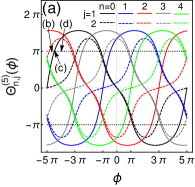
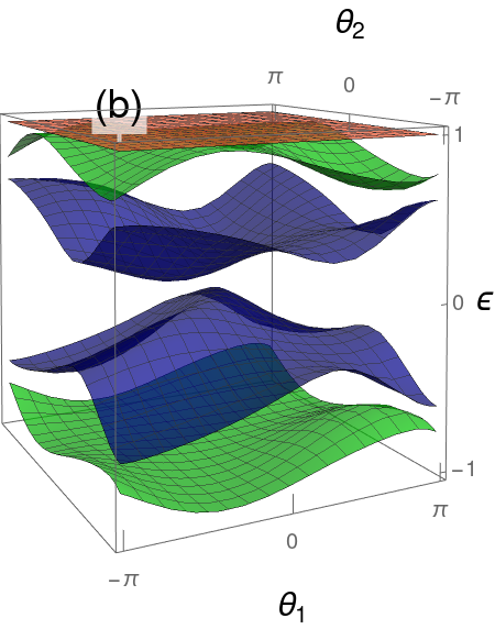
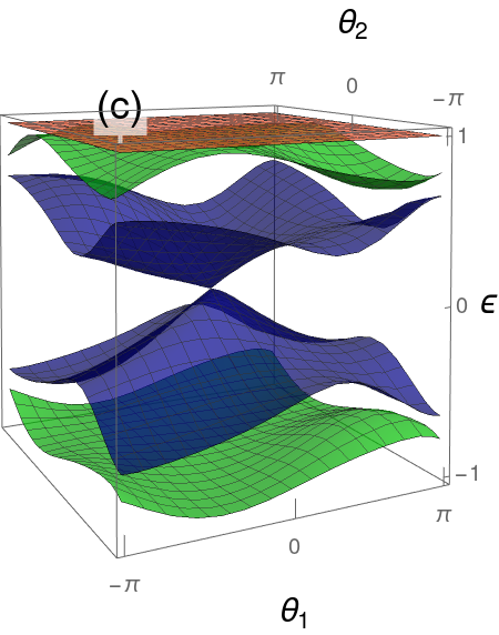
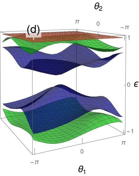
Figure 1: ABS spectrum for a model example of $N=5$ terminal Josephson junction for various $\phi$ and fixed $\mu$ and $t$. We take $\mu=1$ and $t=1.6$ [Eqs. (10) and (15)]. There is one trivial branch at ${\epsilon}=1$. (a) Phase differences $\{\Theta_{n,j}^{(5)}\}$ in Eq. (16) as functions of $\phi$. (b)-(d) ABS spectrum as a function of $\theta_{1,2}$ for $\theta_{3,4}=0$ for various values of $\phi$ as labeled in panel (a). (b) $\phi=-14.2$. (c) $\phi\approx-14.0301$. A Dirac node forms at $\theta_{1,2}=0$. (d) $\phi=-13.8$.

(ii) For the even number of terminals ($N\geq 4$), the result is distinguished by the even and odd values of $n$,

$$T_{n,p}^{{N}}=\begin{cases}2+2\displaystyle\sum_{j=1}^{\mathsf{N}-1}\cos\left[p\,\Theta_{n,j}^{(N,\mathrm{e})}\right],\quad&n\in\mathrm{even},\\ 2\displaystyle\sum_{j=0}^{\mathsf{N}-1}\cos\left[p\,\Theta_{n,j}^{(N,\mathrm{o})}\right],\quad&n\in\mathrm{odd},\end{cases}$$ (17)

where $\mathsf{N}\equiv N/2$, $\Theta_{n,j}^{(N,\mathrm{e})}=d_{\langle\frac{n}{2}+j\rangle}-d_{\langle\frac{n}{2}-j\rangle}$, and $\Theta_{n,j}^{(N,\mathrm{o})}=d_{\langle\frac{n+1}{2}+j\rangle}-d_{\langle\frac{n-1}{2}-j\rangle}$. Specifically, for $N=6$ a zero-energy Dirac point forms at $\hat{\theta}^{(n)}$ when $\Theta_{n,j}^{(6,\mathrm{e}/\mathrm{o})}=\pm\pi$. We depict $\{\Theta_{n,j}^{(6,\mathrm{e}/\mathrm{o})}\}$ as functions of $\phi$ for fixed $\mu$ and $t$ in Fig. 2(a). For the specific values of $\mu$, $t$, and $\phi$, a monopole forms at $\bm{\theta}=0$ and we show the Andreev spectrum in Figs. 2(b)–2(d). We note that alternatively one could set $\phi\to 0$ and vary the parameter space defined by $\mu$ and $t$ to achieve a topological regime.

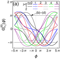
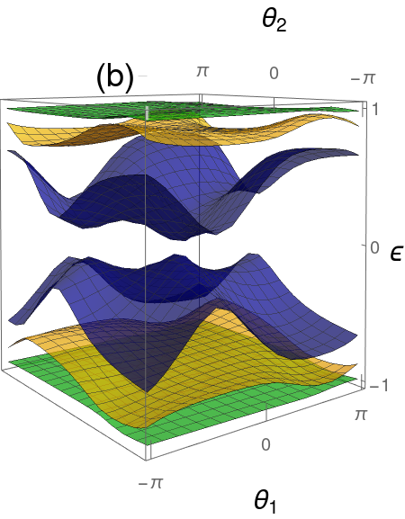
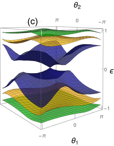
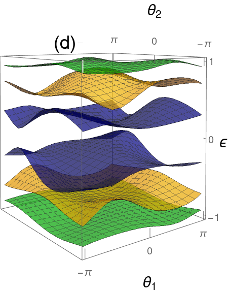
Figure 2: ABS spectrum of $N=6$ terminal Josephson junctions for a fixed $s$ matrix. (a) Phase differences $\{\Theta_{n,j}^{(6)}\}$ in Eq. (17) as functions of $\phi$. A Yang monopole forms at $\bm{\theta}=0$ for $\mu=t=1$ and $\phi\approx-3.7699$. (b)-(d) ABS spectrum as a function of $\theta_{1,2}$ for $\theta_{4,5}=0$ for various values of $\theta_{3}$. (b) $\theta_{3}=-\pi/3$. (c) $\theta_{3}=0$. The monopole manifests. (d) $\theta_{3}=\pi/3$.

II.2 Second Chern number

We proceed to study the topological phases of five -and six-terminal junctions characterized by the second Chern number of the Andreev bound states $\{|\Phi_{n}^{\kappa}(\bm{\theta})\rangle\}$, that are the eigenstates of the Hamiltonian (8). For $N\geq 5$, we define the states on a four-dimensional torus $\theta_{1\leq\alpha\leq 4}\in[0,2\pi]$ and consider the remaining SC phases $\theta_{\alpha\geq 5}$ as fixed parameters if $N>5$. For the $n$th band, we can define the U(2) Berry connection Wilczek and Zee (1984),

$$\mathcal{A}_{n,\alpha}^{\kappa\kappa^{\prime}}(\bm{\theta})\equiv-i\big{\langle}\Phi_{n}^{\kappa}\big{|}\partial_{\alpha}\big{|}\Phi_{n}^{\kappa^{\prime}}\big{\rangle},\quad\kappa,\kappa^{\prime}=1,2,$$ (18)

where $\partial_{\alpha}\equiv\partial_{\theta_{\alpha}}$, which can be decomposed into U(1) and SU(2) parts as $\hat{\mathcal{A}}_{n,\alpha}=(\mathfrak{a}_{n,\alpha}^{0}\hat{\kappa}^{0}+\mathfrak{a}_{n,\alpha}^{j}\hat{\kappa}^{j})/2$ and the U(1) part vanishes $\mathfrak{a}_{n,\alpha}^{0}=0$ in the case of time-reversal symmetry. The corresponding Berry curvature is defined as

$$\hat{\mathcal{F}}_{n,\alpha\beta}\equiv\partial_{\alpha}\hat{\mathcal{A}}_{n,\beta}-\partial_{\beta}\hat{\mathcal{A}}_{n,\alpha}+i\big{[}\hat{\mathcal{A}}_{n,\alpha},\hat{\mathcal{A}}_{n,\beta}\big{]}=\frac{\mathfrak{f}_{n,\alpha\beta}^{j}}{2}\hat{\kappa}_{j},$$ (19)

where $\mathfrak{f}_{n,\alpha\beta}^{j}=\partial_{\alpha}\mathfrak{a}_{n,\beta}^{j}-\partial_{\beta}\mathfrak{a}_{n,\alpha}^{j}-\varepsilon^{jkl}\mathfrak{a}_{n,\alpha}^{k}\mathfrak{a}_{n,\beta}^{l}$. With these notations we can explore the analogy with the Yang-Mills gauge theory and introduce the second Chern number of the $n$ band that reads Belavin et al. (1975); Witten (1977); Yang (1978)

$$\mathcal{C}^{[n]}_{2}\equiv\oint_{\bm{\theta}}\!\varepsilon^{\alpha\beta\gamma\delta}\mathop{\rm Tr}\nolimits\big{[}\hat{\mathcal{F}}_{n,\alpha\beta}\hat{\mathcal{F}}_{n,\gamma\delta}\big{]}=\oint_{\bm{\theta}}\!\varepsilon^{\alpha\beta\gamma\delta}\frac{\mathfrak{f}_{n,\alpha\beta}^{j}\mathfrak{f}_{n,\gamma\delta}^{j}}{2}.$$ (20)

where $\varepsilon^{\alpha\beta\gamma\delta}$ is the Levi-Civita symbol and the sum runs over repeated indices, and $\oint_{\bm{\theta}}\equiv\int_{0}^{2\pi}\!\frac{d^{4}\bm{\theta}}{32\pi^{2}}$. For $N=5$ terminal junctions, the topologies of the gapped Andreev bands are classified by the second Chern number Eq. (20), which is analogous to the 4D quantum Hall effect. For $N=6$ terminal junctions we expect that SU(2) Yang monopoles form in the 5D Andreev bands by tuning the parameters of the $\hat{s}$-matrix.

III Transport signals

The current operator through the $\alpha$th lead is defined by $I_{\alpha}(\bm{\theta})\equiv(2e/\hbar)\partial_{\alpha}H(\bm{\theta})$. In the presence of constant voltages $\{V_{\alpha}\}$ applied to the leads, the SC phases vary linearly in time according to the second Josephson relation $\dot{\theta}_{\alpha}(t)=(2e/\hbar)V_{\alpha}$. The instantaneous eigenenergies and eigenstates are given by the ABS spectrum $\{E_{n}(\bm{\theta}(t))\}$ and wave functions $\{|\Phi_{n}(\bm{\theta}(t))\rangle\}$, respectively. We expand a wave function in the interaction representation

$$\left|\Psi(t)\right\rangle=\sum_{n,\kappa}e^{i\Theta_{n}(t)}c_{n}^{\kappa}(t)|\Phi_{n}^{\kappa}(\bm{\theta}(t))\rangle,$$ (21)

where $\Theta_{n}(t)=-\frac{1}{\hbar}\int_{0}^{t}\!dt^{\prime}E_{n}(\bm{\theta}(t^{\prime}))$ is the dynamical phase, so that the Schrödinger equation takes the form

$$\dot{c}_{n}^{\kappa}(t)= \,-\sum_{\kappa^{\prime}}\langle\Phi_{n}^{\kappa}|\dot{\Phi}_{n}^{\kappa^{\prime}}\rangle c_{n}^{\kappa^{\prime}}(t)$$

$$\,-\frac{\hbar}{2e}\sum_{n^{\prime}\neq n,\kappa^{\prime}}c_{n^{\prime}}^{\kappa^{\prime}}(t)e^{i[\Theta^{n^{\prime}}(t)-\Theta^{n}(t)]}\frac{\dot{\theta}_{\alpha}I_{\alpha,nn^{\prime}}^{\kappa\kappa^{\prime}}}{E_{n^{\prime}}-E_{n}},$$ (22)

where $I_{\alpha,nn^{\prime}}^{\kappa\kappa^{\prime}}\equiv\langle\Phi_{n}^{\kappa}|I_{\alpha}|\Phi_{n^{\prime}}^{\kappa^{\prime}}\rangle$ is the current matrix element in the instantaneous basis (see the Appendix A for further details). In the gapped phase, we impose the adiabatic condition $\mathrm{max}\{2eV_{\alpha}\}\ll\mathrm{min}\{E_{n}-E_{n^{\prime}}\}_{n\neq n^{\prime}}$ and obtain

$$\dot{c}_{n}(t)=-i\dot{\theta}_{\alpha}\hat{\mathcal{A}}_{n,\alpha}\,c_{n}(t),$$ (23)

where $c_{n}(t)\equiv(c_{n}^{1}(t),c_{n}^{2}(t))$ is a two-spinor in the degenerate space. The equation of motion Eq. (23) leads to $\partial_{\alpha}c_{n}=-i\hat{\mathcal{A}}_{n,\alpha}\,c_{n}$, and, therefore, the non-Abelian nature of the Berry connection is manifested by $i[\partial_{\alpha},\partial_{\beta}]c_{n}(t)=\hat{\mathcal{F}}_{\alpha\beta}c_{n}(t)$ in the interaction representation. The adiabatic time evolution gives $c_{n}(t)=\hat{U}_{n}(t)c_{n}(0)$, where

$$\hat{U}_{n}(t)\equiv\mathsf{P}e^{-i\int_{\bm{\theta}(0)}^{\bm{\theta}(t)}\!d\theta_{\alpha}\,\hat{\mathcal{A}}_{n,\alpha}(\bm{\theta})},$$ (24)

with “$\mathsf{P}$” denoting the path order along the trajectory in $\bm{\theta}$ space.

We assume an initial state that is the eigenstate of $H(\bm{\theta}(0))$ of energy $E_{n}(\bm{\theta}(0))$ as well as the adiabatic evolution [Eqs. (21) and (23)]. The instantaneous current through lead $\alpha$ reads $\mathcal{I}_{n,\alpha}(t)\equiv\langle\Psi^{n}(t)|I_{\alpha}(\bm{\theta}(t))|\Psi^{n}(t)\rangle$, and by Eqs. (21) and (23) we obtain

$$\mathcal{I}_{n,\alpha}(t)=J_{n,\alpha}(\bm{\theta}(t))+2e\big{\langle}\hat{\mathcal{F}}_{n,\alpha\beta}\big{\rangle}\dot{\theta}_{\beta},$$ (25)

where $J_{n,\alpha}(\bm{\theta})\equiv\frac{2e}{\hbar}\partial_{\alpha}E_{n}(\bm{\theta})$ is the supercurrent and $\langle\cdots\rangle\equiv c_{n}^{\dagger}(t)\cdots c_{n}(t)$ is the quantum mechanical average at time $t$. We note that the average Berry curvature contributes to the normal current and the instantaneous transconductance. Moreover, if we keep only $V_{2}$ finite and the other voltages vanishing, the time-averaged current, $\bar{\mathcal{I}}_{1}=\mathcal{G}_{12}V_{2},$ gives quantized transconductance, $\mathcal{G}_{12}=(4e^{2}/h)\mathcal{C}_{1}$, that is proportional to the first Chern number $\mathcal{C}_{1}$ defined in the $\theta_{1,2}$ space, as extensively analyzed in earlier works Eriksson et al. (2017); Xie et al. (2018); Meyer and Houzet (2021).

In analogy to Eq. (25), the second Chern number is related to the time average of the instantaneous current correlation function $\mathcal{R}_{n,\alpha\beta}(t)\equiv\langle\Psi^{n}(t)|\Delta I_{\alpha}^{n}\,\Delta I_{\beta}^{n}|\Psi^{n}(t)\rangle$ with $\Delta I_{\alpha}^{n}(t)\equiv I_{\alpha}^{n}(t)-J_{\alpha}^{n}(t)$. We thus obtain

$$\mathcal{R}_{n,\alpha\beta}(t)=4e^{2}\big{\langle}\hat{\mathcal{F}}_{n,\alpha\gamma}\hat{\mathcal{F}}_{n,\beta\delta}\big{\rangle}\dot{\theta}_{\gamma}\dot{\theta}_{\delta}.$$ (26)

In the adiabatic limit, time averaging is equivalent to the integration through the entire phase space. We thus use the Josephson relation for dynamical phases and average autocorrelation function over $\bm{\theta}$. However, unlike in the case of a linear response, where already nonlocal conductance captures topological charge, a nonlinear response requires knowledge of all the nonlocal autocorrelations and only their properly symmetrized sum gives access to higher-rank topologies. Indeed, by combining Eqs. (20) and (26) we can extract

$$\varepsilon^{\alpha\beta\gamma\delta}\frac{\partial^{2}\bar{\mathcal{R}}_{\alpha\beta}}{\partial V_{\gamma}\partial V_{\delta}}=\left(\frac{4\pi e}{\phi_{0}}\right)^{2}\mathcal{C}_{2},$$ (27)

where the fundamental quantization unit is expressed via the flux quantum $\phi_{0}=h/2e$. This result tacitly assumes that in the expectation value for the average of the product of currents the cross-level terms give subleading contributions. Only then can the final result be expressed solely in terms of $\mathcal{C}_{2}$. At finite temperatures occupation functions of the bands would also enter the result. We expect that the robustness of the quantization will be also limited by the voltage/phase noise. With the simplest assumption of white noise in the voltage sources leading to fluctuating phases, $\langle\delta\theta_{\alpha}(t)\delta\theta_{\beta}(t^{\prime})\rangle=\Upsilon\delta_{\alpha\beta}\delta(t-t^{\prime})$, described by a single broadening energy scale $\Upsilon$, one can estimate that the required measurement time to sufficiently average the current signals must exceed $(\Delta/eV)^{2}\Upsilon^{-1}$. Other limiting factors include Landau-Zener transitions between the bands and to the continuum of states above the gap leading to the dissipation. Finally, we note that phase dynamics can be described with the help of the Fokker-Planck equation that in particular yields the probability distribution function of phases. We leave a detailed analysis of these complications to the future work.

Appendix A Adiabatic approximation

In this section we sketch the derivation of the current correlation functions. The adiabatic approximation introduced in the Schrödinger equation (22) implies that $\mathcal{A}_{nn^{\prime},\alpha}^{\kappa\kappa^{\prime}}$ is dominated by the diagonal blocks $n=n^{\prime}$, so that we introduce the formal decomposition $\hat{\mathcal{A}}_{nn^{\prime},\alpha}=\delta_{nn^{\prime}}\hat{\mathcal{A}}_{n,\alpha}+\lambda(1-\delta_{nn^{\prime}})\hat{a}_{nn^{\prime},\alpha}$ where $\lambda\hat{a}_{nn^{\prime},\alpha}=\hat{\mathcal{A}}_{nn^{\prime},\alpha}$ and $\lambda\ll 1$. We define instantaneous eigenstates of the Hamiltonian

$$|\eta_{n}^{\kappa}(t)\rangle\equiv e^{i\Theta_{n}(t)}\sum_{\kappa^{\prime}}U_{n}^{\kappa^{\prime}\kappa}(t)|\Phi_{n}^{\kappa^{\prime}}(\bm{\theta}(t))\rangle,$$ (28)

where $\hat{U}(t)$ is the adiabatic evolution operator in Eq. (24). These satisfy the orthonormal condition $\langle\eta_{n^{\prime}}^{\kappa^{\prime}}(t)|\eta_{n}^{\kappa}(t)\rangle=\delta_{nn^{\prime}}\delta_{\kappa\kappa^{\prime}}$ and the completeness condition $1=|\eta_{n}^{\kappa}(t)\rangle\langle\eta_{n}^{\kappa}(t)|$. For an arbitrary state in Eq. (21) we have

$$\langle\eta_{n}^{\kappa}(t)|\Psi(t)\rangle=(\hat{U}_{n}^{\dagger}c_{n})^{\kappa}.$$ (29)

Moreover, we obtain the important relations

$$i\hbar|\dot{\eta}_{n}^{\kappa}\rangle=E_{n}|\eta_{n}^{\kappa}\rangle+i\hbar\dot{\theta}_{\alpha}\partial_{\alpha}|\eta_{n}^{\kappa}\rangle,$$

$$i\partial_{\alpha}|\eta_{n}^{\kappa}\rangle=e^{i\Theta_{n}(t)}\sum_{\kappa^{\prime}}\big{[}(\hat{\mathcal{A}}_{n}\hat{U}_{n})^{\kappa^{\prime}\kappa}+U_{n}^{\kappa^{\prime}\kappa}i\partial_{\alpha}\big{]}|\Phi_{n}^{\kappa^{\prime}}\rangle.$$ (30)

In the basis (28), the matrix elements of the current operator reads

$$\langle\eta_{n^{\prime}}^{\kappa^{\prime}}|I_{\alpha}|\eta_{n}^{\kappa}\rangle \approx\frac{2e}{\hbar}\big{[}\delta_{nn^{\prime}}\delta_{\kappa\kappa^{\prime}}\partial_{\alpha}E_{n}$$

$$-i\hbar\langle\partial_{\alpha}\eta_{n^{\prime}}^{\kappa^{\prime}}|\dot{\eta}_{n}^{\kappa}\rangle+i\hbar\langle\dot{\eta}_{n^{\prime}}^{\kappa^{\prime}}|\partial_{\alpha}\eta_{n}^{\kappa}\rangle\big{]},$$ (31)

where we have used the adiabatic approximation of the form $H|\eta_{n}^{\kappa}\rangle\approx i\hbar|\dot{\eta}_{n}^{\kappa}\rangle+\mathcal{O}(\lambda)$. Applying the relations in Eq. (30) to Eq. (31), we find

$$\langle\eta_{n^{\prime}}^{\kappa^{\prime}}|I_{\alpha}|\eta_{n}^{\kappa}\rangle\approx\delta_{nn^{\prime}}\left[\hat{U}_{n}^{\dagger}\left(J_{\alpha}^{n}+2e\dot{\theta}_{\beta}\hat{\mathcal{F}}_{n,\alpha\beta}\right)\hat{U}_{n}\right]^{\kappa^{\prime}\kappa},$$ (32)

that is block diagonal up to small corrections in adiabaticity. Using the completeness condition with Eqs. (29) and (32), we obtain Eqs. (25) and (26). It is further possible to extend the calculation of the instantaneous current correlations to higher-order cumulants.

References

- Chern (1946) Shiing-shen Chern, “Characteristic classes of hermitian manifolds,” Annals of Mathematics 47, 85–121 (1946).
- Thouless et al. (1982) D. J. Thouless, M. Kohmoto, M. P. Nightingale, and M. den Nijs, “Quantized hall conductance in a two-dimensional periodic potential,” Phys. Rev. Lett. 49, 405–408 (1982).
- Yang (1978) Chen Ning Yang, “Generalization of dirac’s monopole to su2 gauge fields,” Journal of Mathematical Physics 19, 320–328 (1978).
- Zhang and Hu (2001) Shou-Cheng Zhang and Jiangping Hu, “A four-dimensional generalization of the quantum hall effect,” Science 294, 823–828 (2001).
- Murakami et al. (2003) Shuichi Murakami, Naoto Nagaosa, and Shou-Cheng Zhang, “Dissipationless quantum spin current at room temperature,” Science 301, 1348–1351 (2003).
- Kraus et al. (2013) Yaacov E. Kraus, Zohar Ringel, and Oded Zilberberg, “Four-dimensional quantum hall effect in a two-dimensional quasicrystal,” Phys. Rev. Lett. 111, 226401 (2013).
- Chern et al. (2004) Chyh-Hong Chern, Han-Dong Chen, Congjun Wu, Jiang-Ping Hu, and Shou-Cheng Zhang, “Non-abelian berry phase and chern numbers in higher spin-pairing condensates,” Phys. Rev. B 69, 214512 (2004).
- Sugawa et al. (2018) Seiji Sugawa, Francisco Salces-Carcoba, Abigail R. Perry, Yuchen Yue, and I. B. Spielman, “Second chern number of a quantum-simulated non-abelian yang monopole,” Science 360, 1429–1434 (2018).
- Kolodrubetz (2016) Michael Kolodrubetz, “Measuring the second chern number from nonadiabatic effects,” Phys. Rev. Lett. 117, 015301 (2016).
- Riwar et al. (2016) Roman-Pascal Riwar, Manuel Houzet, Julia S. Meyer, and Yuli V. Nazarov, “Multi-terminal josephson junctions as topological matter,” Nature Communications 7, 11167 (2016).
- Eriksson et al. (2017) Erik Eriksson, Roman-Pascal Riwar, Manuel Houzet, Julia S. Meyer, and Yuli V. Nazarov, “Topological transconductance quantization in a four-terminal josephson junction,” Phys. Rev. B 95, 075417 (2017).
- Xie et al. (2017) Hong-Yi Xie, Maxim G. Vavilov, and Alex Levchenko, “Topological andreev bands in three-terminal josephson junctions,” Phys. Rev. B 96, 161406 (2017).
- Meyer and Houzet (2017) Julia S. Meyer and Manuel Houzet, “Nontrivial chern numbers in three-terminal josephson junctions,” Phys. Rev. Lett. 119, 136807 (2017).
- Xie et al. (2018) Hong-Yi Xie, Maxim G. Vavilov, and Alex Levchenko, “Weyl nodes in andreev spectra of multiterminal josephson junctions: Chern numbers, conductances, and supercurrents,” Phys. Rev. B 97, 035443 (2018).
- Deb et al. (2018) Oindrila Deb, K. Sengupta, and Diptiman Sen, “Josephson junctions of multiple superconducting wires,” Phys. Rev. B 97, 174518 (2018).
- Erdmanis et al. (2018) Janis Erdmanis, Árpád Lukács, and Yuli V. Nazarov, “Weyl disks: Theoretical prediction,” Phys. Rev. B 98, 241105 (2018).
- Houzet and Meyer (2019) Manuel Houzet and Julia S. Meyer, “Majorana-weyl crossings in topological multiterminal junctions,” Phys. Rev. B 100, 014521 (2019).
- Xie and Levchenko (2019) Hong-Yi Xie and Alex Levchenko, “Topological supercurrents interaction and fluctuations in the multiterminal josephson effect,” Phys. Rev. B 99, 094519 (2019).
- Kotetes et al. (2019) Panagiotis Kotetes, Maria Teresa Mercaldo, and Mario Cuoco, “Synthetic weyl points and chiral anomaly in majorana devices with nonstandard andreev-bound-state spectra,” Phys. Rev. Lett. 123, 126802 (2019).
- Stenger and Pekker (2019) John P. T. Stenger and David Pekker, “Weyl points in systems of multiple semiconductor-superconductor quantum dots,” Phys. Rev. B 100, 035420 (2019).
- Kornich et al. (2019) Viktoriia Kornich, Hristo S. Barakov, and Yuli V. Nazarov, “Fine energy splitting of overlapping andreev bound states in multiterminal superconducting nanostructures,” Phys. Rev. Research 1, 033004 (2019).
- Peralta Gavensky et al. (2019) Lucila Peralta Gavensky, Gonzalo Usaj, and C. A. Balseiro, “Topological phase diagram of a three-terminal josephson junction: From the conventional to the majorana regime,” Phys. Rev. B 100, 014514 (2019).
- Marra and Nitta (2019) Pasquale Marra and Muneto Nitta, “Topologically nontrivial andreev bound states,” Phys. Rev. B 100, 220502 (2019).
- Repin et al. (2019) E. V. Repin, Y. Chen, and Y. V. Nazarov, “Topological properties of multiterminal superconducting nanostructures: Effect of a continuous spectrum,” Phys. Rev. B 99, 165414 (2019).
- Sakurai et al. (2020) Keimei Sakurai, Maria Teresa Mercaldo, Shingo Kobayashi, Ai Yamakage, Satoshi Ikegaya, Tetsuro Habe, Panagiotis Kotetes, Mario Cuoco, and Yasuhiro Asano, “Nodal andreev spectra in multi-majorana three-terminal josephson junctions,” Phys. Rev. B 101, 174506 (2020).
- Douçot et al. (2020) Benoît Douçot, Romain Danneau, Kang Yang, Jean-Guy Caputo, and Régis Mélin, “Berry phase in superconducting multiterminal quantum dots,” Phys. Rev. B 101, 035411 (2020).
- Klees et al. (2020) R. L. Klees, G. Rastelli, J. C. Cuevas, and W. Belzig, “Microwave spectroscopy reveals the quantum geometric tensor of topological josephson matter,” Phys. Rev. Lett. 124, 197002 (2020).
- Meyer and Houzet (2021) Julia S. Meyer and Manuel Houzet, “Conductance quantization in topological josephson trijunctions,” Phys. Rev. B 103, 174504 (2021).
- Fatemi et al. (2021) Valla Fatemi, Anton R. Akhmerov, and Landry Bretheau, “Weyl josephson circuits,” Phys. Rev. Research 3, 013288 (2021).
- Chirolli and Moore (2021) Luca Chirolli and Joel E. Moore, “Enhanced coherence in superconducting circuits via band engineering,” Phys. Rev. Lett. 126, 187701 (2021).
- Peyruchat et al. (2021) L. Peyruchat, J. Griesmar, J.-D. Pillet, and Ç. Ö. Girit, “Transconductance quantization in a topological josephson tunnel junction circuit,” Phys. Rev. Research 3, 013289 (2021).
- Repin and Nazarov (2020) E. V. Repin and Y. V. Nazarov, “Weyl points in the multi-terminal Hybrid Superconductor-Semiconductor Nanowire devices,” arXiv e-prints (2020), arXiv:2010.11494 [cond-mat.mes-hall] .
- Septembre et al. (2020) Ismael Septembre, Sergei Koniakhin, Julia Meyer, Dmitry Solnyshkov, and Guillaume Malpuech, “Parametric amplification of topological interface states in synthetic Andreev bands,” arXiv e-prints (2020), arXiv:2012.05709 [cond-mat.mes-hall] .
- Chen and Nazarov (2021) Y. Chen and Y. V. Nazarov, “Weyl point immersed in a continuous spectrum: an example from superconducting nanostructures,” arXiv e-prints (2021), arXiv:2102.03947 [cond-mat.mes-hall] .
- Mélin (2021) Régis Mélin, “The dc-Josephson effect with more than four superconducting leads,” arXiv e-prints (2021), arXiv:2103.03519 [cond-mat.supr-con] .
- Weisbrich et al. (2021a) H. Weisbrich, R.L. Klees, G. Rastelli, and W. Belzig, “Second chern number and non-abelian berry phase in topological superconducting systems,” PRX Quantum 2, 010310 (2021a).
- Weisbrich et al. (2021b) H. Weisbrich, M. Bestler, and W. Belzig, “Tensor monopoles in superconducting systems,” Quantum 5, 601 (2021b).
- Pachos et al. (1999) Jiannis Pachos, Paolo Zanardi, and Mario Rasetti, “Non-abelian berry connections for quantum computation,” Phys. Rev. A 61, 010305 (1999).
- Pekola et al. (1999) J. P. Pekola, J. J. Toppari, M. Aunola, M. T. Savolainen, and D. V. Averin, “Adiabatic transport of cooper pairs in arrays of josephson junctions,” Phys. Rev. B 60, R9931–R9934 (1999).
- Leone et al. (2008) R. Leone, L. P. Lévy, and P. Lafarge, “Cooper-pair pump as a quantized current source,” Phys. Rev. Lett. 100, 117001 (2008).
- Strambini et al. (2016) E. Strambini, S. D’Ambrosio, F. Vischi, F. S. Bergeret, Yu. V. Nazarov, and F. Giazotto, “The ω-squipt as a tool to phase-engineer josephson topological materials,” Nature Nanotechnology 11, 1055–1059 (2016).
- Draelos et al. (2019) Anne W. Draelos, Ming-Tso Wei, Andrew Seredinski, Hengming Li, Yash Mehta, Kenji Watanabe, Takashi Taniguchi, Ivan V. Borzenets, François Amet, and Gleb Finkelstein, “Supercurrent flow in multiterminal graphene josephson junctions,” Nano Letters, Nano Letters 19, 1039–1043 (2019).
- Arnault et al. (2020) Ethan G. Arnault, Trevyn Larson, Andrew Seredinski, Lingfei Zhao, Hengming Li, Kenji Watanabe, Takashi Taniguchi, Ivan V. Borzenets, Francois Amet, and Gleb Finkelstein, “The Multi-terminal Inverse AC Josephson Effect,” arXiv e-prints (2020), arXiv:2012.15253 [cond-mat.mes-hall] .
- Cohen et al. (2018) Yonatan Cohen, Yuval Ronen, Jung-Hyun Kang, Moty Heiblum, Denis Feinberg, Régis Mélin, and Hadas Shtrikman, “Nonlocal supercurrent of quartets in a three-terminal josephson junction,” Proceedings of the National Academy of Sciences 115, 6991–6994 (2018).
- Pankratova et al. (2020) Natalia Pankratova, Hanho Lee, Roman Kuzmin, Kaushini Wickramasinghe, William Mayer, Joseph Yuan, Maxim G. Vavilov, Javad Shabani, and Vladimir E. Manucharyan, “Multiterminal josephson effect,” Phys. Rev. X 10, 031051 (2020).
- Graziano et al. (2020) Gino V. Graziano, Joon Sue Lee, Mihir Pendharkar, Chris J. Palmstrøm, and Vlad S. Pribiag, “Transport studies in a gate-tunable three-terminal josephson junction,” Phys. Rev. B 101, 054510 (2020).
- Graziano et al. (arXiv e-prints 2022) Gino V. Graziano, Mohit Gupta, Mihir Pendharkar, Jason T. Dong, Connor P. Dempsey, Chris Palmstrøm, and Vlad S. Pribiag, “Selective control of conductance modes in multi-terminal josephson junctions,” (arXiv e-prints 2022).
- Beenakker (2015) C. W. J. Beenakker, “Random-matrix theory of majorana fermions and topological superconductors,” Rev. Mod. Phys. 87, 1037–1066 (2015).
- Beenakker (1991) C. W. J. Beenakker, “Universal limit of critical-current fluctuations in mesoscopic josephson junctions,” Phys. Rev. Lett. 67, 3836–3839 (1991).
- van Heck et al. (2014) B. van Heck, S. Mi, and A. R. Akhmerov, “Single fermion manipulation via superconducting phase differences in multiterminal josephson junctions,” Phys. Rev. B 90, 155450 (2014).
- Altland and Zirnbauer (1997) Alexander Altland and Martin R. Zirnbauer, “Nonstandard symmetry classes in mesoscopic normal-superconducting hybrid structures,” Phys. Rev. B 55, 1142–1161 (1997).
- Wilczek and Zee (1984) Frank Wilczek and A. Zee, “Appearance of gauge structure in simple dynamical systems,” Phys. Rev. Lett. 52, 2111–2114 (1984).
- Belavin et al. (1975) A.A. Belavin, A.M. Polyakov, A.S. Schwartz, and Yu.S. Tyupkin, “Pseudoparticle solutions of the yang-mills equations,” Physics Letters B 59, 85–87 (1975).
- Witten (1977) Edward Witten, “Some exact multipseudoparticle solutions of classical yang-mills theory,” Phys. Rev. Lett. 38, 121–124 (1977).