A Deep Residual Star Generative Adversarial Network for multi-domain Image Super-Resolution

Abstract

Recently, most of state-of-the-art single image super-resolution (SISR) methods have attained impressive performance by using deep convolutional neural networks (DCNNs). The existing SR methods have limited performance due to a fixed degradation settings, i.e. usually a bicubic downscaling of low-resolution (LR) image. However, in real-world settings, the LR degradation process is unknown which can be bicubic LR, bilinear LR, nearest-neighbor LR, or real LR. Therefore, most SR methods are ineffective and inefficient in handling more than one degradation settings within a single network. To handle the multiple degradation, i.e. refers to multi-domain image super-resolution, we propose a deep Super-Resolution Residual StarGAN (SR${}^{2~{}*}$GAN), a novel and scalable approach that super-resolves the LR images for the multiple LR domains using only a single model. The proposed scheme is trained in a StarGAN like network topology with a single generator and discriminator networks. We demonstrate the effectiveness of our proposed approach in quantitative and qualitative experiments compared to other state-of-the-art methods.

I Introduction

The goal of the single image super-resolution (SISR) is to reconstruct the high-resolution (HR) image from its low-resolution (LR) image counterpart. SISR problem is a fundamental low-level vision and image processing problem with various practical applications in satellite imaging, medical imaging, video enhancement and security and surveillance imaging as well. With the increasing amount of HR images / videos data on the internet, there is a great demand for storing, transferring, and sharing such large sized data with low cost of storage and bandwidth resources. Moreover, the HR images are usually downscaled to easily fit into display screens with different resolutions while retaining visually plausible information. The downscaled LR counterpart of the HR can efficiently utilize lower bandwidth, save storage, and easily fit to various digital displays. However, some details are lost and sometimes visible artifacts appear when users downscale and upscale the digital contents.

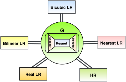
Figure 1: The visualization of our proposed approach where a single generator $\mathbf{G}$ learns the mappings among multiple domains i.e. LR/HR to LR/HR.

Usually, the SISR is described as a linear forward observation model [1, 2, 3] by the following image degradation process:

$${\bf y}={\bf H}*\tilde{{\bf x}}+\eta,$$ (1)

where ${\bf y}$ is an observed LR image, ${\bf H}$ is a down-sampling operator that convolves with an HR image $\tilde{{\bf x}}$ and resizes it by a scaling factor $s$, and $\eta$ is considered as an additive white Gaussian noise with standard deviation $\sigma$. However, in real-world settings, $\eta$ also accounts for all possible errors during the image acquisition process that include inherent sensor noise, stochastic noise, compression artifacts, and the possible mismatch between the forward observation model and the camera device. In most of existing SR methods, the operator ${\bf H}$ is usually known / fixed i.e. bicubic. But in real-world settings, the operator ${\bf H}$ is unknown that can be bicubic, bilinear, nearest, and real degradation kernel.

Recently, numerous works have been addressed toward the task of SISR that are based on DCNNs for their powerful feature representation capabilities either on PSNR values [4, 5, 6, 7, 8, 9, 10] or on visual quality [11, 12, 13, 14, 1, 2]. The SR methods mostly rely on the single degradation (i.e. usually bicubic) with paired LR and HR images in the supervised training. In the real-world settings, the input LR image contains more complex degradation. As the bicubic, bilinear, and nearest LR degradation are rarely suitable for the real LR images, but these degradations can be used for data augmentation and are indeed a good choice for clean and sharp image super-resolution. Moreover, the Real LR domain in the proposed method contains the LR/HR image pairs that follow the realistic physical image model instead of artificial ones. Due to such different degradation settings, the most SR methods often fail to produce convincing SR results or train their model independently for every pair of image domains.

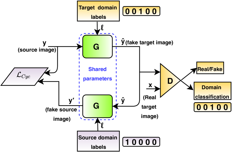
Figure 2: Visualizes the structure of the our proposed SR${}^{2~{}*}$GAN setup. $\mathbf{G}$ takes an input as both the source image (${\bf y}$) and target domain label and generates a fake target image ($\hat{{\bf y}}$). $\mathbf{G}$ tries to reconstruct the fake source image (${\bf y}^{\prime}$) from the fake target image ($\hat{{\bf y}}$) given the source domain label. $\mathbf{D}$ learns to discriminate between real and fake target images and classify the real target images to its corresponding domain. In this way, the $\mathbf{G}$ tries to generate fake target images indistinguishable from real target images and classifiable as target domain images by the $\mathbf{D}$.

Instead of learning a fixed degradation setting (e.g., bicubic LR), the proposed SR${}^{2~{}*}$GAN  takes as inputs both an image and a domain label, and learns to generate the image into the corresponding domain (LR/HR). The domain labels are encoded in binary or one-hot vector to represent domain information. Fig. 1 illustrates an overview of our proposed SISR approach, where a single network $\mathbf{G}$ learns the mappings among the multiple domains i.e. Bicubic LR, Bilinear LR, Nearest LR, Real LR, and HR. During the training phase, we translate the source domain images into the target domain images by randomly generate target domain labels. At the testing phase, we fix the target domain as HR domain to generate the SR images from any blind LR domain. The proposed scheme is inspired by the recent success of StarGAN [15] for multi-domain image-to-image translation applications. The proposed approach (refers to the section III for more details) allows us to simultaneously train for multiple domains with in a unified network.

Our contributions in this paper are as follows:

• We propose SR${}^{2~{}*}$GAN  for multi-domain image super-resolution task. In contrast to the existing deep SISR methods, our method learns the mappings among multiple domains with in a single model.

• The proposed scheme requires a single generator and discriminator networks to train efficiently for the images of multiple domains.

• We provide both qualitative and quantitative results on SR benchmarks to show its superiority over existing SR methods.

II Related Work

Recently, numerous works addressed the task of SISR using deep CNNs for their powerful feature representation capabilities. A preliminary CNN-based method to solve SISR is a super-resolution convolutional network with three layers (SRCNN) [16]. Kim et al. [4] proposed a very deep SR (VDSR) network with a residual learning approach. Lim et al. [5] proposed an enhanced deep SR (EDSR) network by taking advantage of the residual learning. In [17], the authors proposed SRWDNet to solve the joint deblurring and super-resolution task by following the realistic degradation. In [3], the authors proposed the ISRResCNet to solve the SISR in an iterative manner. These methods mostly rely on the PSNR-based metric by optimizing the $\mathcal{L}_{1}$/$\mathcal{L}_{2}$ losses in a supervised way by the LR/HR paired data.

For the perception SR task, a preliminary attempt was made by Ledig et al. [11] who proposed the SRGAN method to produce perceptually more pleasant results. To further enhance the performance of the SRGAN, Wang et al. [12] proposed the ESRGAN model to achieve the state-of-art perceptual performance. Despite their success, the previously mentioned methods are trained with LR/HR image pairs with the bicubic downsampling and thus they have limited performance in the real-world settings. Recently, in the real-world SR challenge series [18, 19, 20], the authors have described the effects of bicubic downsampling. More recently, in [1, 2], the authors proposed GAN-based SR methods to solve the real-world SR problem. However, the above SR methods have different models to be independently built for every LR degradation. Our approach takes into account the different LR degradation within a single network by greatly increasing its applicability in practical scenarios.

III Proposed Method

III-A Multi-domain training strategy

Our goal is to train a single network $\mathbf{G}$ that super-resolves the LR images from multiple LR domains. To achieve this objective, we train the generator $\mathbf{G}$ to translate an input source image ${\bf y}$ into an output target image $\hat{{\bf y}}$ conditioned on the target domain labels $\mathbf{\ell}$ as $\mathbf{G}({\bf y},\mathbf{\ell})\rightarrow\hat{{\bf y}}$. The domain labels $\mathbf{\ell}$ are encoded in binary or one-hot vector to represent domain information. We randomly generate the target domain labels $\mathbf{\ell}$ so that the network $\mathbf{G}$ flexibly translates the source domain images into the target domain images. The discriminator network $\mathbf{D}$ learns to distinguish between real/fake images and also tries to minimize the domain classification error only associated with the known domain label. The discriminator $\mathbf{D}$ (i.e. adapted from StarGAN [15]) produces the probability distributions over both target images and target domain labels, $\mathbf{D}:{\bf x}\rightarrow\{\mathbf{D}_{trg}({\bf x}),\mathbf{D}_{cls}({\bf x})\}$. Fig. 2 illustrates the training strategy of the proposed SR${}^{2~{}*}$GAN.

III-B Network Architectures

Generator ($\mathbf{G}$): We use the generator $\mathbf{G}$ network as a Encoder-Resnet-Decoder like structure, adapted from SRResCGAN [1] which strictly follows the degradation process (1). In the $\mathbf{G}$ network, both Encoder and Decoder layers have $64$ convolutional feature maps of $5\times 5$ kernel size with $C\times H\times W$ tensors, where $C$ is the number of channels of the input image. Resnet consists of $5$ residual blocks with two Pre-activation Conv layers, each of $64$ feature maps with kernel support $3\times 3$, and the preactivation is the Sine nonlinearities layer with $64$ output feature channels. The trainable projection layer [21] inside the Decoder computes the proximal map with the estimated noise standard deviation $\sigma$ and handles the data fidelity and prior terms.
Discriminator ($\mathbf{D}$): The discriminator network ($\mathbf{D}$) learns to distinguish between real and fake images and classify the real images to its corresponding domain. The discriminator network contains 6 convolutional layers with kernels that support $4\times 4$ of increasing feature maps from $64$ to $2048$ followed by the leaky ReLU as done in StarGAN [15].

III-C Network Losses

To train the generator $\mathbf{G}$ and discriminator $\mathbf{D}$, we use the following respective objective loss functions:

$$\mathcal{L}_{G}=\mathcal{L}_{\mathrm{per}}+\mathcal{L}_{\mathrm{GAN}}+\mathcal{L}_{tv}+\mathcal{L}_{cls}^{f}+10\cdot\mathcal{L}_{\mathrm{1}}+10\cdot\mathcal{L}_{\mathrm{cyc}},$$ (2)

$$\mathcal{L}_{D}=\mathcal{L}_{GAN}+\mathcal{L}_{cls}^{r},$$ (3)

where $\mathcal{L}_{per}$, $\mathcal{L}_{GAN}$, $\mathcal{L}_{tv}$, $\mathcal{L}_{cls}^{r/f}$, $\mathcal{L}_{1}$, and $\mathcal{L}_{cyc}$ denote the perceptual (VGG-based) loss, texture/GAN loss, total variation loss, real/fake classification loss, content loss, and cyclic loss respectively.

IV Experiments

IV-A Training data

For the training, we use DIV2K [22], Flickr2K [23], and RealSR [24] datasets that jointly contain 22,430 high-quality HR images for image restoration tasks with rich and diverse textures. We obtain the LR bicubic, LR bilinear, and LR nearest images by down-sampling HR images by the scaling factor $\times 4$ of the DIV2K and Flickr2K datasets using the Pytorch bicubic, bilinear, and nearest kernel function. The LR real images by the scaling factor $\times 4$ are provided with their corresponding HR images in the RealSR dataset. We consider the five domains as shown in Fig. 1. We obtain the source domain images from the three datasets with their corresponding domain labels. We randomly generate the target domain labels with their corresponding images from the three datasets. We train our network in RGB color space.

IV-B Data augmentation

We augment the training data with random vertical and horizontal flipping, and $90^{\circ}$ rotations. Moreover, we also consider another effective data augmentation technique, called mixture of augmentation (MOA) [25] strategy. In the MOA, a data augmentation (DA) method, among i.e. Blend, RGB permutation, Mixup, Cutout, Cutmix, Cutmixup, and CutBlur is randomly selected and then applied on the inputs. This MOA technique encourages the network to acquire more generalization power by partially blocking or corrupting the training sample.

IV-C Training details

At the training time, we set the input image patch size as $128\times 128$. We train the network for 51000 training iterations with a batch size of 16 using Adam optimizer with parameters $\beta_{1}=0.9$, $\beta_{2}=0.999$, and $\epsilon=10^{-8}$ without weight decay for both generator and discriminator to minimize the loss functions in the Eqs. (2) and (3). The learning rate is initially set to $10^{-4}$ and then multiplies by $0.5$ after 5K, 10K, 20K, and 30K iterations. Our all experiments are performed with a scaling factor of $\times 4$ for the LR and HR images.

TABLE I: $\times 4$ SR quantitative results comparison of our method with others over the DIV2K (100 images of validation-set) and RealSR (93 images of testset) that are total 393 images of the testset with the four LR degradation. The arrows indicate if high $\uparrow$ or low $\downarrow$ values are desired. The best performance is shown in red and the second best performance is shown in blue.

SR methods	#Params	Bicubic	Bilinear	Nearest	Real	Average
		PSNR$\uparrow$ / SSIM$\uparrow$ / LPIPS$\downarrow$	PSNR$\uparrow$ / SSIM$\uparrow$ / LPIPS$\downarrow$	PSNR$\uparrow$ / SSIM$\uparrow$ / LPIPS$\downarrow$	PSNR$\uparrow$ / SSIM$\uparrow$ / LPIPS$\downarrow$	PSNR$\uparrow$ / SSIM$\uparrow$ / LPIPS$\downarrow$
EDSR [5]	$43M$	21.33 / 0.66 / 0.3477	23.05 / 0.72 / 0.3083	19.34 / 0.56 / 0.3653	28.06 / 0.82 / 0.4182	22.95 / 0.69 / 0.3599
ESRGAN [12]	$16.7M$	16.02 / 0.31 / 0.6008	17.25 / 0.37 / 0.5186	15.29 / 0.26 / 0.6254	27.98 / 0.82 / 0.3840	19.14 / 0.44 / 0.5322
SRResCGAN [1]	$380K$	23.30 / 0.67 / 0.2900	24.43 / 0.70 / 0.2720	21.10 / 0.60 / 0.3044	27.96 / 0.82 / 0.3676	24.20 / 0.69 / 0.3085
SRResCycGAN [2]	$380K$	24.56 / 0.73 / 0.3380	25.58 / 0.75 / 0.3183	21.75 / 0.63 / 0.3541	28.02 / 0.82 / 0.3827	24.98 / 0.73 / 0.3483
SR${}^{2~{}*}$GAN  (ours)	$380K$	25.52 / 0.75 / 0.4250	26.23 / 0.76 / 0.4083	22.75 / 0.66 / 0.4415	28.02 / 0.82 / 0.4353	25.63 / 0.75 / 0.4275

IV-D Evaluation metrics

We evaluate the trained model under the Peak Signal-to-Noise Ratio (PSNR), Structural Similarity (SSIM), and LPIPS [26] metrics. The PSNR and SSIM are distortion-based measures, while the LPIPS better correlates with human perception. We measure the LPIPS based on the features of pretrained AlexNet [26]. The quantitative SR results are evaluated on the $RGB$ color space.

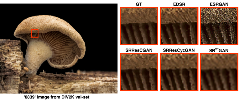
(a) SR results on the LR bicubic

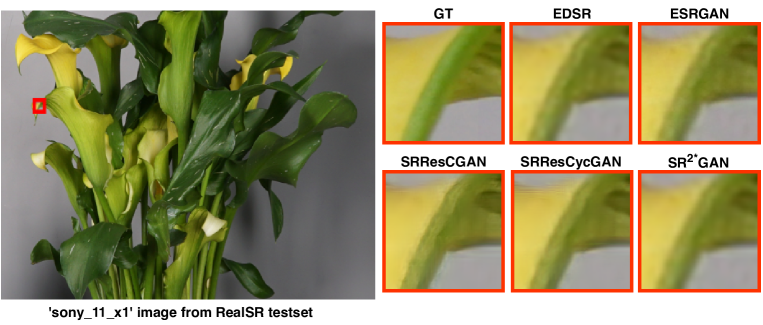
(b) SR results on the LR real

Figure 3: Visual comparison of our method with other state-of-art methods on $\times 4$ super-resolution.

IV-E Comparison with the state-of-art methods

We compare our method with other state-of-art SISR methods including EDSR [5], ESRGAN [12], SRResCGAN [1], and SRResCycGAN [2]. We compare the SR results with one deep feed-forward residual network (i.e. EDSR) and other three GAN-based approaches (i.e. ESRGAN, SRResCGAN, SRResCycGAN). Although there are existing SR methods [7], [10], and [17] by handling multiple degradation settings, but they are the non-blind SR techniques with deep feed-forward networks, while our proposed method is a blind SR GAN-based approach. So, the comparison with [7], [10], and [17] methods is not fair. We run all the original source codes and trained models by the default parameters settings for the comparison. The competing methods are trained for just one degradation setting and tested on the different ones. Unlike them, the proposed approach can be trained with multiple degradations instead of single degradation.

Table I shows the quantitative results comparison of our method with the others over the DIV2K (100 images of validation-set) and RealSR (93 images of testset) that are total 393 images of the testset with the four LR degradation. We have excellent results in terms of PSNR and SSIM compared to the other methods, while in the case of LPIPS, we lag by the others because our training objective is to get better PSNR/SSIM. The reason for none of the competing methods achieved their best performance against the bicubic down-sampling, is that the other GAN-based approaches focus more on the perceptual quality, as good perceptual image quality reduces the PSNR/SSIM scores. Our model is trained with reasonably perceptual quality, while good PSNR/SSIM, refers to section IV-F.

Regarding the visual quality, Fig. 3 shows the visual comparison of our method with other SR methods at the $\times 4$ upscaling factor on the test-set. We have comparable visual SR results with others.

TABLE II: This table reports the quantitative SR results of our method over the DIV2K and RealSR validation-set (20 images, not used during the training phase) with the four LR domains (i.e. Bicubic, Bilinear, Nearest, Real) for our ablation study. The arrows indicate if high $\uparrow$ or low $\downarrow$ values are desired.

SR method	Domain label Conditioning ($\ell$)	PSNR$\uparrow$	SSIM$\uparrow$	LPIPS$\downarrow$
SR${}^{2~{}*}$GAN  (v1)	$\mathbf{G}$ Conditioned on only HR target domain & used two separate Disc. ($\mathbf{D}_{trg}$, $\mathbf{D}_{src}$)	26.95	0.75	0.3423
SR${}^{2~{}*}$GAN  (v2)	$\mathbf{G}$ Conditioned on only HR target domain & used one Disc. ($\mathbf{D}_{trg}$)	27.20	0.76	0.3176
SR${}^{2~{}*}$GAN  (v3)	$\mathbf{G}$ Conditioned on random target domains & used one Disc. ($\mathbf{D}_{trg}$)	28.09	0.78	0.3891

IV-F Ablation Study

For our ablation study, we train three variants of the proposed SR${}^{2~{}*}$GAN  network structure with conditioning of the domain labels. By referencing to the Fig. 2, the first network variant v1 is trained by conditioning the first branch generator $\mathbf{G}$ on only HR target domain labels, while, the other branch generator $\mathbf{G}$ (shared weights) is conditioned on the multiple LR source domain labels. We use two separate discriminators i.e. $\mathbf{D}_{trg}$ for the target domain supervision, $\mathbf{D}_{src}$ for the source domain supervision in the SR${}^{2~{}*}$GAN  (v1). Similarly, the second network variant v2 is trained as the v1, but only uses one discriminator i.e. $\mathbf{D}_{trg}$ for the target domain supervision. Finally, the third network variant v3 is trained by conditioning both generators $\mathbf{G}$ on random domain labels and use only one discriminator $\mathbf{D}_{trg}$ for the real target domain supervision by minimizing the the total loss functions in the Eqs. (2) and (3). Table II shows the quantitative SR results of SR${}^{2~{}*}$GAN  (v1, v2, v3) over the DIV2K and RealSR validation-sets (20 images, not used during the training phase) with the four LR domains i.e. Bicubic, Bilinear, Nearest, Real. The third network variant v3 performs better in terms of PSNR/SSIM among others. This shows the effectiveness of random target domain labeling and real target domain images supervision by the discriminator. Therefore, we opt for the third version v3 and used it for the evaluation in the section-IV-E.

V Conclusion

We proposed a unified deep SR${}^{2~{}*}$GAN  for the multi-domain image super-resolution task. The proposed scheme learns the multiple degradation of different domains within a single model. The proposed method trains the single generator and discriminator networks to efficiently learn mappings among multiple domains using StarGAN like network topology. Our method achieves excellent SR results in terms of the PSNR/SSIM values compared to the existing SR methods.

References

- [1] R. Muhammad Umer, G. Luca Foresti, and C. Micheloni, “Deep generative adversarial residual convolutional networks for real-world super-resolution,” in CVPRW, 2020, pp. 438–439.
- [2] R. Muhammad Umer and C. Micheloni, “Deep cyclic generative adversarial residual convolutional networks for real image super-resolution,” in ECCVW, August 2020.
- [3] R. Muhammad Umer, G. Luca Foresti, and C. Micheloni, “Deep iterative residual convolutional network for single image super-resolution,” in ICPR, January 2021.
- [4] J. Kim, J. K. Lee, and K. M. Lee, “Accurate image super-resolution using very deep convolutional networks,” CVPR, pp. 1646–1654, 2016.
- [5] B. Lim, S. Son, H. Kim, S. Nah, and K. M. Lee, “Enhanced deep residual networks for single image super-resolution,” CVPRW, pp. 1132–1140, 2017.
- [6] K. Zhang, W. Zuo, S. Gu, and L. Zhang, “Learning deep cnn denoiser prior for image restoration,” CVPR, pp. 2808–2817, 2017.
- [7] K. Zhang, W. Zuo, and L. Zhang, “Learning a single convolutional super-resolution network for multiple degradations,” CVPR, pp. 3262–3271, 2018.
- [8] Y. Yuan, S. Liu, J. Zhang, Y. Zhang, C. Dong, and L. Lin, “Unsupervised image super-resolution using cycle-in-cycle generative adversarial networks,” in CVPRW, 2018, pp. 701–710.
- [9] Y. Li, J. Yang, Z. Liu, X. Yang, G. Jeon, and W. Wu, “Feedback network for image super-resolution,” CVPR, 2019.
- [10] K. Zhang, W. Zuo, and L. Zhang, “Deep plug-and-play super-resolution for arbitrary blur kernels,” in CVPR, 2019, pp. 1671–1681.
- [11] C. Ledig et al., “Photo-realistic single image super-resolution using a generative adversarial network,” in CVPR, 2017, pp. 4681–4690.
- [12] X. Wang, K. Yu, S. Wu, J. Gu, Y. Liu, C. Dong, Y. Qiao, and C. Change Loy, “ESRGAN: Enhanced super-resolution generative adversarial networks,” in ECCV, 2018.
- [13] A. Lugmayr, M. Danelljan, and R. Timofte, “Unsupervised learning for real-world super-resolution,” ICCVW, 2019.
- [14] M. Fritsche, S. Gu, and R. Timofte, “Frequency separation for real-world super-resolution,” ICCVW, 2019.
- [15] Y. Choi, M. Choi, M. Kim, J.-W. Ha, S. Kim, and J. Choo, “StarGAN: Unified generative adversarial networks for multi-domain image-to-image translation,” in CVPR, 2018, pp. 8789–8797.
- [16] C. Dong, C. C. Loy, K. He, and X. Tang, “Learning a deep convolutional network for image super-resolution,” ECCV, pp. 184–199, 2014.
- [17] R. M. Umer, G. L. Foresti, and C. Micheloni, “Deep super-resolution network for single image super-resolution with realistic degradations,” in ICDSC, September 2019, pp. 21:1–21:7.
- [18] A. Lugmayr, M. Danelljan, R. Timofte et al., “AIM 2019 challenge on real-world image super-resolution: Methods and results,” in ICCVW, 2019.
- [19] A. Lugmayr, M. Danelljan, and R. Timofte, “NTIRE 2020 challenge on real-world image super-resolution: Methods and results,” in CVPRW, June 2020.
- [20] P. Wei, H. Lu, R. Timofte et al., “AIM 2020 challenge on real image super-resolution: Methods and results,” in ECCVW, August 2020.
- [21] S. Lefkimmiatis, “Universal denoising networks: A novel cnn architecture for image denoising,” CVPR, pp. 3204–3213, 2018.
- [22] E. Agustsson and R. Timofte, “Ntire 2017 challenge on single image super-resolution: Dataset and study,” in CVPRW, 2017, pp. 126–135.
- [23] R. Timofte, E. Agustsson, L. Van Gool, M.-H. Yang, and L. Zhang, “Ntire 2017 challenge on single image super-resolution: Methods and results,” in CVPRW, 2017, pp. 114–125.
- [24] P. Wei, H. Lu, R. Timofte, L. Lin, W. Zuo et al., “AIM 2020 challenge on real image super-resolution: Methods and results,” in ECCVW, August 2020.
- [25] J. Yoo, N. Ahn, and K.-A. Sohn, “Rethinking data augmentation for image super-resolution: A comprehensive analysis and a new strategy,” in CVPR, 2020, pp. 8375–8384.
- [26] R. Zhang, P. Isola, A. A. Efros, E. Shechtman, and O. Wang, “The unreasonable effectiveness of deep features as a perceptual metric,” in CVPR, 2018, pp. 586–595.