O

Abstract

Contextual bandits are a rich model for sequential decision making given side information, with important applications, e.g., in recommender systems. We propose novel algorithms for contextual bandits harnessing neural networks to approximate the unknown reward function. We resolve the open problem of proving sublinear regret bounds in this setting for general context sequences, considering both fully-connected and convolutional networks. To this end, we first analyze NTK-UCB, a kernelized bandit optimization algorithm employing the Neural Tangent Kernel (NTK), and bound its regret in terms of the NTK maximum information gain $\gamma_{T}$, a complexity parameter capturing the difficulty of learning. Our bounds on $\gamma_{T}$ for the NTK may be of independent interest. We then introduce our neural network based algorithm NN-UCB, and show that its regret closely tracks that of NTK-UCB. Under broad non-parametric assumptions about the reward function, our approach converges to the optimal policy at a $\tilde{\mathcal{O}}(T^{-1/2d})$ rate, where $d$ is the dimension of the context.

 

Neural Contextual Bandits without Regret

 

Parnian Kassraie                        Andreas Krause ETH Zurich pkassraie@ethz.ch                        ETH Zurich krausea@ethz.ch

1 Introduction

Contextual bandits are a model for sequential decision making based on noisy observations. At every step, the agent is presented with a context vector and picks an action, based on which it receives a noisy reward. Learning about the reward function with few samples (exploration), while simultaneously maximizing its cumulative payoff (exploitation), are the agent’s two competing objectives. Our goal is to develop an algorithm whose action selection policy attains sublinear regret, which implies convergence to an optimal policy as the number of observations grows. A celebrated approach for regret minimization is the optimism principle: establishing upper confidence bounds (UCB) on the reward, and always selecting a plausibly optimal action. Prior work has developed UCB-based contextual bandit approaches, such as linear or kernelized bandits, for increasingly rich models of reward functions (Abbasi-Yadkori et al., 2011; Auer, 2002; Chowdhury and Gopalan, 2017; Srinivas et al., 2010). There are also several recent attempts to harness deep neural networks for contextual bandit tasks. While these perform well in practice (Gu et al., 2021; Riquelme et al., 2018; Nabati et al., 2021; ZHANG et al., 2021; Zhou et al., 2020), there is a lack of theoretical understanding of neural network-based bandit approaches.

We introduce two optimistic contextual bandit algorithms that employ neural networks to estimate the reward and its uncertainty, NN-UCB and its convolutional variant CNN-UCB. Under the assumption that the unknown reward function $f$ resides in a Reproducing Kernel Hilbert Space (RKHS) with a bounded norm, we prove that both algorithms converge to the optimal policy, if the network is sufficiently wide, or has many channels. To prove this bound, we take a two-step approach. We begin by bounding the regret for NTK-UCB, which simply estimates mean and variance of the reward via Gaussian process (GP) inference. Here, the covariance function of the GP is set to ${k_{\mathrm{NN}}}$, the Neural Tangent Kernel associated with the given architecture. We then exploit the fact that neural networks trained with gradient descent approximate the posterior mean of this GP (Arora et al., 2019), and generalize our analysis of NTK-UCB to bound NN-UCB’s regret. By drawing a connection between fully-connected and 2-layer convolutional networks, we extend our analysis to include CNTK-UCB and CNN-UCB, the convolutional variants of the algorithms. A key contribution of our work is bounding the NTK maximum information gain, a parameter that measures the difficulty of learning about a reward function when it is a sample from $\mathrm{GP}(0,{k_{\mathrm{NN}}})$. This result may be of independent interest, as this quantity is integral to sequential decision making approaches.

Related Work

This work is inspired by Zhou et al. (2020) who introduce the idea of training a neural network within a UCB style algorithm. They analyze Neural-UCB, which bears many similarities to NN-UCB. Relevant treatments of the regret are given by Gu et al. (2021); Yang et al. (2020), ZHANG et al. (2021), and Ban and He (2021) for other neural contextual bandit algorithms. However, as discussed in Section 4, these approaches do not generally guarantee sublinear regret, unless further restrictive assumptions about the context are made. In addition, there is a large literature on kernelized contextual bandits. Closely related to our work are Krause and Ong (2011) and Valko et al. (2013) who provide regret bounds for kernelized UCB methods, with Bayesian and Frequentist perspectives respectively. Srinivas et al. (2010) are the first to tackle the kernelized bandit problem with a UCB based method. Many have then proposed variants of this algorithm, or improved its convergence guarantees under a variety of settings (Berkenkamp et al., 2021; Bogunovic et al., 2020; Calandriello et al., 2019; Chowdhury and Gopalan, 2017; Djolonga et al., 2013; Kandasamy et al., 2019; Mutnỳ and Krause, 2019; Scarlett, 2018). The majority of the bounds in this field are expressed in terms of the maximum information gain, and Srinivas et al. (2010) establish a priori bounds on this parameter. Their analysis only holds for smooth kernel classes, but has since been extended to cover more complex kernels (Janz et al., 2020; Scarlett et al., 2017; Shekhar et al., 2018; Vakili et al., 2021a). In particular, Vakili et al. (2021a) introduce a technique that applies to smooth Mercer kernels, which we use as a basis for our analysis of the NTK’s maximum information gain. In parallel to UCB methods, online decision making via Thompson Sampling is also extensively studied following Russo and Van Roy (2016).

Our work further builds on the literature linking wide neural networks and Neural Tangent Kernels. Cao and Gu (2019) provide important results on training wide fully-connected networks with gradient descent, which we extend to 2-layer convolutional neural networks (CNNs). Through a non-asymptotic bound, Arora et al. (2019) approximate a trained neural network by the posterior mean of a GP with the NTK as its covariance function. Bietti and Bach (2021) study the Mercer decomposition of the NTK and calculate the decay rate of its eigenvalues, which plays an integral role in our analysis. Little is known about the properties of the Convolutional Neural Tangent Kernel (CNTK), and the extent to which it can be used for approximating trained CNNs. Bietti (2022) and Mei et al. (2021) are among the first to study this kernel by investigating its invariance towards certain groups of transformations, which we draw inspiration from.

Contributions

Our main contributions are:

• To our knowledge, we are the first to give an explicit sublinear regret bound for a neural network based UCB algorithm. We show that NN-UCB’s cumulative regret after a total of $T$ steps is $\tilde{{\mathcal{O}}}(T^{(2d-1)/2d})$, for any arbitrary context sequence on the $d$-dimensional hyper-sphere. (Theorem 4.2)

• We introduce CNN-UCB, and prove that when the number of channels is large enough, it converges to the optimal policy at the same rate as NN-UCB. (Theorem 5.4)

The $\tilde{\mathcal{O}}$ notation omits the terms of order $\log T$ or slower. Along the way, we present intermediate results that may be of independent interest. In Theorem 3.1 we prove that $\gamma_{T}$, the maximum information gain for the NTK after $T$ observations, is $\tilde{\mathcal{O}}(T^{(d-1)/d})$. We introduce and analyze NTK-UCB and CNTK-UCB, two kernelized methods with sublinear regret (Theorems 3.2 & 3.3) that can be used in practice or as a theoretical tool. Theorems 3.1 through 3.3 may provide an avenue for extending other kernelized algorithms to neural network based methods.

2 Problem Statement

Contextual bandits are a model of sequential decision making over $T$ rounds, where, at step $t$, the learner observes a context matrix ${\bm{z}}_{t}$, and picks an action ${\bm{a}}_{t}$ from $\mathcal{A}$, the finite set of actions. The context matrix consists of a set of vectors, one for each action, i.e., ${\bm{z}}_{t}=({\bm{z}}_{t,1},\cdots,{\bm{z}}_{t,|\mathcal{A}|})\in\mathbb{R}^{d\times|\mathcal{A}|}$. The learner then receives a noisy reward $y_{t}=f({\bm{x}}_{t})+\epsilon_{t}$. Here, the input to the reward function is the context vector associated with the chosen action, i.e., ${\bm{x}}_{t}={\bm{z}}_{t}{\bm{a}}_{t}\in{\mathbb{R}}^{d}$, where ${\bm{a}}_{t}$ is represented as a one-hot vector of length $|\mathcal{A}|$. Then the reward function is defined as $f:\mathcal{X}\rightarrow{\mathbb{R}}$, where $\mathcal{X}\subseteq\mathbb{R}^{d}$ denotes the input space. Observation noise is modeled with $\epsilon_{t}$, an i.i.d. sample from a zero-mean sub-Gaussian distribution with variance proxy $\sigma^{2}>0$. The goal is to choose actions that maximize the cumulative reward over $T$ time steps. This is analogous to minimizing the cumulative regret, the difference between the maximum possible (context-dependent) reward and the actual reward received, $R_{T}=\sum_{t=1}^{T}f({\bm{x}}_{t}^{*})-f({\bm{x}}_{t})$, where ${\bm{x}}_{t}$ is the learner’s pick and ${\bm{x}}^{*}_{t}$ is the maximizer of the reward function at step $t$

$${\bm{x}}^{*}_{t}=\operatorname*{arg\,max}_{{\bm{x}}={\bm{z}}_{t}{\bm{a}},{\bm{a}}\in\mathcal{A}}f({\bm{x}}).$$

The learner’s goal is to select actions such that $R_{T}/T\rightarrow 0$ as $T\rightarrow\infty$. This property implies that the learner’s policy will converge to the optimal policy.

2.1 Assumptions

Our regret bounds require some assumptions on the reward function $f$ and the input space $\mathcal{X}$. Throughout this work, we assume that $\mathcal{A}$ is finite and $\mathcal{X}$ is a subset of $\mathbb{S}^{d-1}$ the $d$-dimensional unit hyper-sphere. We consider two sets of assumptions on $f$,

• Frequentist Setting: We assume that $f$ is an arbitrary function residing in $\mathcal{H}_{k_{\mathrm{NN}}}$ the RKHS that is reproducing for the NTK, and has a bounded kernel norm, $\left\lVert f\right\rVert_{k_{\mathrm{NN}}}\leq B$.

• Bayesian Setting: We assume that $f$ is a sample from a zero-mean Gaussian process, that uses the NTK as its covariance function, $\text{GP}(0,{k_{\mathrm{NN}}})$.

These assumptions are broad, non-parametric and imply that $f$ is continuous on the hyper-sphere. Both the Bayesian and the Frequentist setting impose certain smoothness properties on $f$ via ${k_{\mathrm{NN}}}$. Technically, the function class addressed by each assumption has an empty intersection with the other. Appendix B.1 provides more insight into the connection between the two assumptions. We require a mild Sufficient Exploration assumption on the kernel matrix, exclusive to the results in Sections 4 and 5. This is presented later, under Assumption 4.1.

2.2 The Neural Tangent Kernel

We review important properties of the NTK as relied upon in this work. Training very wide neural networks has similarities to estimation with kernel methods using the NTK. For now, we will focus on fully-connected feed-forward ReLU networks and their corresponding NTK. In Section 5, we extend our result to networks with one convolutional layer. Let $f({\bm{x}};{\bm{\theta}}):\mathbb{R}^{d}\rightarrow\mathbb{R}$ be a fully-connected network, with $L$ hidden layers of equal width $m$, and ReLU activations, recursively defined as follows,

$$\begin{split}f^{(1)}({\bm{x}})&={\bm{W}}^{(1)}{\bm{x}},\\ f^{(l)}({\bm{x}})&=\sqrt{\frac{2}{m}}{\bm{W}}^{(l)}\sigma_{\text{relu}}\big{(}f^{(l-1)}({\bm{x}})\big{)}\in\mathbb{R}^{m},\,\,1<l\leq L\\ f({\bm{x}};{\bm{\theta}})&=\sqrt{2}{\bm{W}}^{(L+1)}\sigma_{\text{relu}}\big{(}f^{(L)}({\bm{x}})\big{)}\in{\mathbb{R}}.\end{split}$$

The weights ${\bm{W}}^{(i)}$ are initialized to random matrices with standard normal i.i.d. entries, and ${\bm{\theta}}=({\bm{W}}^{(i)})_{i\leq L+1}$. Let ${\bm{g}}({\bm{x}};{\bm{\theta}})=\nabla_{\bm{\theta}}f({\bm{x}};{\bm{\theta}})$ be the gradient of $f$. Assume that given a fixed dataset, the network is trained with gradient descent using an infinitesimally small learning rate. For networks with large width $m$, training causes little change in the parameters and, respectively, the gradient vector. For any ${\bm{x}},\,{\bm{x}}^{\prime}\in\mathcal{X}$, and as $m$ tends to infinity, a limiting behavior emerges: $\langle{\bm{g}}({\bm{x}};{\bm{\theta}}),{\bm{g}}({\bm{x}}^{\prime};{\bm{\theta}})\rangle/m$, the inner product of the gradients, remains constant during training and converges to ${k_{\mathrm{NN}}}({\bm{x}};{\bm{x}}^{\prime})$, a deterministic kernel function (Arora et al., 2019; Jacot et al., 2018). This kernel satisfies the conditions of Mercer’s Theorem over ${\mathbb{S}}^{d-1}$ with the uniform measure (Cao et al., 2021) and has the following Mercer decomposition,

$${k_{\mathrm{NN}}}({\bm{x}},{\bm{x}}^{\prime})=\sum_{k=0}^{\infty}\mu_{k}\sum_{j=1}^{N(d,k)}Y_{j,k}({\bm{x}})Y_{j,k}({\bm{x}}^{\prime}),$$ (1)

where $Y_{j,k}$ is the $j$-th spherical harmonic polynomial of degree $k$, and $N(d,k)$ denotes the algebraic multiplicity of $\mu_{k}$. In other words, each $\mu_{k}$ corresponds to a $N(d,k)$ dimensional eigenspace, where $N(d,k)$ grows with $k^{d-2}$. Without loss of generality, assume that the distinct eigenvalues $\mu_{k}$ are in descending order. Bietti and Bach (2021) show that there exists an absolute constant ${C(d,L)}$ such that

$$\mu_{k}\simeq{C(d,L)}k^{-d}.$$ (2)

Taking the algebraic multiplicity into account, we obtain that the decay rate for the complete spectrum of eigenvalues is of polynomial rate $k^{-1-1/(d-1)}$. This decay is slower than that of the kernels commonly used for kernel methods. The eigen-decay for the squared exponential kernel is $O(\exp(-k^{1/d}))$ (Belkin, 2018), and Matérn kernels with smoothness $\nu>1/2$ have a $O(k^{-1-2\nu/d})$ decay rate (Santin and Schaback, 2016). The RKHS associated with ${k_{\mathrm{NN}}}$ is then given by

$$\mathcal{H}_{k_{\mathrm{NN}}}=\Big{\{}f:\,f=\sum_{k\geq 0}\sum_{j=1}^{N(d,k)} \beta_{j,k}Y_{j,k},$$ (3)

$$\sum_{k\geq 0}\sum_{j=1}^{N(d,k)}\frac{\beta_{j,k}^{2}}{\mu_{k}}<\infty\Big{\}}.$$

Equation 3 explains how the eigen-decay of $k$ controls the complexity of $\mathcal{H}_{k}$. Only functions whose coefficients $\beta_{j,k}$ decay at a faster rate than the kernel’s eigenvalues are contained in the RKHS. Therefore, if the eigenvalues of $k$ decay rapidly, ${\mathcal{H}}_{k}$ is more limited. The slow decay of the NTK’s eigenvalues implies that the assumptions on the reward function given in Section 2.1 are less restrictive compared to what is often studied in the kernelized contextual bandit literature.

3 Warm-up: NTK-UCB – Kernelized Contextual Bandits with the NTK

Our first step will be to analyze kernelized bandit algorithms that employ the NTK as the kernel. In particular, we focus on the Upper Confidence Bound (UCB) exploration policy (Srinivas et al., 2010). Kernelized bandits can be interpreted as modeling the reward function $f$ via a Bayesian prior, namely a Gaussian process $\text{GP}(0,k)$ with covariance function given by $k$. At each step $t$, we calculate the posterior mean and variance $\mu_{t-1}(\cdot)$ and $\sigma_{t-1}(\cdot)$, using the samples observed at previous steps. For i.i.d.  $\mathcal{N}(0,\sigma^{2})$ noise, the posterior GP has a closed form expression,

$$\mu_{t-1}({\bm{x}}) =\bm{k}_{t-1}^{T}({\bm{x}})(\bm{K}_{t-1}+\sigma^{2}\bm{I})^{-1}{\bm{y}}_{t-1}$$ (4)

$$\sigma^{2}_{t-1}({\bm{x}}) =k({\bm{x}},{\bm{x}})-\bm{k}^{T}_{t-1}({\bm{x}})(\bm{K}_{t-1}+\sigma^{2}\bm{I})^{-1}\bm{k}_{t-1}({\bm{x}})$$

where ${\bm{y}}_{t-1}=[y_{i}]_{i<t}$ is the vector of received rewards, $\bm{k}_{t-1}({\bm{x}})=[k({\bm{x}},{\bm{x}}_{i})]_{i<t}$, and $\bm{K}_{t-1}=[k({\bm{x}}_{i},{\bm{x}}_{j})]_{i,j<t}$ is the kernel matrix. We then select the action by maximizing the UCB,

$${\bm{x}}_{t}=\operatorname*{arg\,max}_{{\bm{x}}={\bm{z}}_{t}{\bm{a}},\,{\bm{a}}\in\mathcal{A}}\mu_{t-1}({\bm{x}})+\sqrt{\beta_{t}}\sigma_{t-1}({\bm{x}}).$$ (5)

The acquisition function balances exploring uncertain actions and exploiting the gained information via parameter $\beta_{t}$ which will be detailed later. Our method NTK-UCB, adopts the UCB approach, and uses ${k_{\mathrm{NN}}}$ as the covariance kernel function of the GP for calculating the posteriors in Equation 4.

3.1 Information Gain

The UCB policy seeks to learn about $f$ quickly, while picking actions that also give big rewards. The speed at which we learn about $f$ is quantified by the maximum information gain. Assume that for a sequence of inputs $X_{T}=({\bm{x}}_{1},\cdots,{\bm{x}}_{T})$, the learner observes noisy rewards ${\bm{y}}_{T}=(y_{1},\dots,y_{T})$, and let ${\bm{f}}_{T}=(f({\bm{x}}_{1}),\dots,f({\bm{x}}_{T}))$ be the corresponding true rewards. Then the information gain is defined as the mutual information between these random vectors, $I({\bm{y}}_{T};{\bm{f}}_{T}):=H({\bm{y}}_{T})-H({\bm{y}}_{T}|{\bm{f}}_{T})$, where $H$ denotes the entropy. Assuming the GP prior $f\sim\text{GP}(0,{k_{\mathrm{NN}}})$, and in the presence of i.i.d. Gaussian noise,

$$I({\bm{y}}_{T};{\bm{f}}_{T})=\frac{1}{2}\log\det(\bm{I}+\sigma^{-2}{\bm{K}}_{T})$$

with the kernel matrix ${\bm{K}}_{T}=[{k_{\mathrm{NN}}}({\bm{x}}_{i},{\bm{x}}_{j})]_{i,j\leq T}$. Following Srinivas et al. (2010), we will express our regret bounds in terms of the information gain. The information gain depends on the sequence of points observed. To obtain bounds for arbitrary context sequences, we work with the maximum information gain defined as $\gamma_{T}:=\max_{X_{T}}I({\bm{y}}_{T};{\bm{f}}_{T})$. By bounding $I({\bm{y}}_{T};{\bm{f}}_{T})$ with $\gamma_{T}$, we obtain regret bounds that are independent of the input sequence.

Many regret bounds in this literature, including ours, are of the form $\tilde{\mathcal{O}}(\sqrt{T\gamma_{T}})$ or $\tilde{\mathcal{O}}(\sqrt{T}\gamma_{T})$. For such a bound not to be vacuous, i.e., for it to guarantee convergence to an optimal policy, $\gamma_{T}$ must grow strictly sub-linearly with $T$. Our first main result is an a priori bound on $\gamma_{T}$ for Neural Tangent Kernels corresponding to fully-connected networks of depth $L$.

Theorem 3.1.

Suppose the observation noise is i.i.d., zero-mean and a Gaussian of variance $\sigma^{2}>0$, and the input domain $\mathcal{X}\subset\mathbb{S}^{d-1}$. Then the maximum information gain associated with the NTK of a fully-connected ReLU network is bounded by $\gamma_{T}=\mathcal{O}\bigg{(}\Big{(}\frac{{C(d,L)}T}{\log(1+\frac{T}{\sigma^{2}})}\Big{)}^{\frac{d-1}{d}}\log\Big{(}1+\frac{T}{\sigma^{2}}\Big{(}\frac{{C(d,L)}T}{\log(1+\frac{T}{\sigma^{2}})}\Big{)}^{\frac{d-1}{d}}\Big{)}\bigg{)}$

The parameter $\gamma_{T}$ arises not only in the bandit setting, but in a broad range of related sequential decision making tasks (Berkenkamp et al., 2021; Kandasamy et al., 2016; Kirschner et al., 2020; Kirschner and Krause, 2019; Sessa et al., 2019, 2020; Sui et al., 2018). Theorem 3.1 might therefore be of independent interest and facilitate the extension of other kernelized algorithms to neural network based methods. When restricted to ${\mathbb{S}}^{d-1}$, the growth rate of $\gamma_{T}$ for the NTK matches the rate for a Matérn kernel with smoothness coefficient of $\nu=1/2$, since both kernels have the same rate of eigen-decay (Chen and Xu, 2021). Srinivas et al. (2010) bound $\gamma_{T}$ for smooth Matérn kernels with $\nu\geq 1$, and Vakili et al. (2021a) extend this result to $\nu>1/2$. From this perspective, Theorem 3.1 pushes the previous literature one step further by bounding the information gain of a kernel with the same eigen-decay as a Matérn kernel with $\nu=1/2$.

Proof Idea

Beyond classical analyses of $\gamma_{T}$, additional challenges arise when working with the NTK, since it does not have the smoothness properties required in prior works. As a consequence, we directly use the Mercer decomposition of the NTK (Eq. 1) and break it into two terms, one corresponding to a kernel with a finite-dimensional feature map, and a tail sum. We separately bound the information gain caused by each term. From the Matérn perspective, we are able to extend the previous results, in particular due to our treatment of the Mercer decomposition tail sum. An integral element of our approach is a fine-grained analysis of the NTK’s eigenspectrum over the hyper-sphere, given by Bietti and Bach (2021). The complete proof is given in Appendix C.1.

3.2 Regret Bounds

We now proceed with bounding the regret for NTK-UCB, under both Bayesian and Frequentist assumptions, as explained in Section 2.1. Following Krause and Ong (2011), and making adjustments where needed, we obtain a bound for the Bayesian setting.

Theorem 3.2.

Let $\delta\in(0,1)$ and suppose $f$ is sampled from $\mathrm{GP}(0,{k_{\mathrm{NN}}})$. Values of $f$ are observed with a zero-mean Gaussian noise of variance $\sigma^{2}$, and the exploration parameter is set to $\beta_{t}=2\log(|\mathcal{A}|t^{2}\pi^{2}/6\delta)$. Then with probability greater than $1-\delta$, the regret of NTK-UCB satisfies

$$R_{T}\leq C\sqrt{T\beta_{T}\gamma_{T}}$$

for any $T\geq 1$, where $C:=\sqrt{8\sigma^{-2}/\log(1+\sigma^{-2})}$.

Crucially, this bound holds for any sequence of observed contexts, since $\gamma_{T}$ is deterministic and only depends on $\sigma$, $T$, the kernel function ${k_{\mathrm{NN}}}$, and the input domain $\mathcal{X}$. A key ingredient in the proofs of regret bounds, including Theorem 3.2, is a concentration inequality of the form

$$\left\lvert f({\bm{x}}_{t})-\mu_{t-1}({\bm{x}}_{t})\right\rvert\leq\sqrt{\beta_{t}}\sigma_{t-1}({\bm{x}}_{t}),$$ (6)

which holds with high probability for every ${\bm{x}}_{t}$ and $t$, conditioned on context-reward pairs from the previous steps. This inequality holds naturally under the GP assumption, since $f({\bm{x}})$ is obtained directly from Bayesian inference. Setting $\beta_{t}$ to grow with $\log t$ satisfies the inequality and results in a $\tilde{\mathcal{O}}(\sqrt{T\gamma_{T}})$ regret bound. However, additional challenges arise under the RKHS assumption. For Equation  6 to hold in this setting, we need $\beta_{t}$ to grow with $\gamma_{t}\log t$. The regret would then be $\tilde{\mathcal{O}}(\sqrt{T}\gamma_{T})$ (Chowdhury and Gopalan, 2017). For NTK-UCB, $\gamma_{T}$ is $\tilde{\mathcal{O}}(T^{(d-1)/d})$, and the $\gamma_{T}\sqrt{T}$ rate would no longer imply convergence to the optimal policy for $d\geq 2$. To overcome this open problem (Vakili et al., 2021b), we analyze a variant of our algorithm – called the Sup variant – that has been successfully applied in the kernelized bandit literature (Auer, 2002; Chu et al., 2011; Li et al., 2010; Valko et al., 2013). A detailed description of the SupNTK-UCB, along with its pseudo-code and properties is given in Appendix C.3. Here we give a high-level overview of the Sup variant, and how it resolves the large $\beta_{t}$ problem. This variant combines NTK-UCB policy with Random Exploration (RE). At NTK-UCB steps, the UCB is calculated only using the context-reward pairs observed in the previous RE steps. Moreover, the rewards received during the RE steps are statistically independent conditioned on the input for those steps. Together with other properties, this allows a choice of $\beta_{t}$ that grows with $\log T$. We obtain the following:

Theorem 3.3.

Let $\delta\in[0,1]$. Suppose $f$ lies in the RKHS of ${k_{\mathrm{NN}}}$, with $||f||_{k_{\mathrm{NN}}}\leq B$. Samples of $f$ are observed with a zero-mean sub-Gaussian noise with variance proxy $\sigma^{2}$. Then for a constant $\beta_{t}=2\log\big{(}2T|\mathcal{A}|/\delta\big{)}$, with probability greater than $1-\delta$, SupNTK-UCB algorithm satisfies

$$\begin{split}R(T)=\mathcal{O}\Big{(}\sqrt{T}\Big{(}&\sqrt{\gamma_{T}\sigma^{-2}(\log T)^{3}\log(T\log T|\mathcal{A}|/\delta)}\\ &+\sigma B\Big{)}\Big{)}.\end{split}$$

The first term corresponds to regret of the random exploration steps, and the second term results from the steps at which the actions were taken by the NTK-UCB policy. Proofs of Theorems 3.2 and 3.3 are given in Appendices  C.2 and C.4 respectively. We finish our analysis of the NTK-UCB with the following conclusion, employing our bound on $\gamma_{T}$ from Theorem 3.1 in Theorems 3.2 and 3.3.

Corollary 3.4.

Suppose $f$ satisfies either the GP or RKHS assumption. Then the NTK-UCB (resp. its Sup variant) has sublinear regret $R(T)=\tilde{\mathcal{O}}({C_{\mathrm{NN}}(d,L)}T^{\frac{2d-1}{2d}})$ with high probability. Hereby, ${C_{\mathrm{NN}}(d,L)}$ is a coefficient depending on the eigen-decay of the NTK.

4 Main Result: NN-UCB – Neural Contextual Bandits without Regret

Having analyzed NTK-UCB, we now present our neural net based algorithm NN-UCB, which leverages the connections between NN training and GP regression with the NTK. By design, NN-UCB benefits from the favorable properties of the kernel method which helps us with establishing our regret bound. NN-UCB results from approximating the posterior mean and variance functions appearing in the UCB criterion (Equation 5). First, we approximate the posterior mean $\mu_{t-1}$ with $f^{(J)}=f({\bm{x}};{\bm{\theta}}^{(J)})$, the neural network trained for $J$ steps of gradient descent with some learning rate $\eta$ with respect to the regularized LSE loss

$$\mathcal{L}({\bm{\theta}})=\sum_{i=1}^{t-1}\big{(}f({\bm{x}}_{i};{\bm{\theta}})-y_{i}\big{)}^{2}+m\sigma^{2}\big{|}\big{|}{\bm{\theta}}-{\bm{\theta}}^{0}\big{|}\big{|}^{2}_{2},$$ (7)

where $m$ is the width of the network and ${\bm{\theta}}^{0}$ denotes the network parameters at initialization. This choice is motivated by Arora et al. (2019), who show point-wise convergence of the solution of gradient descent on the unregularized LSE loss, to the GP posterior mean when there is no observation noise. We adapt their result to our setting where we consider $\ell_{2}$ regularized loss and noisy samples. It remains to approximate the posterior variance. Recall from Section 2.2 that the NTK is the limit of $\langle{\bm{g}}({\bm{x}}),{\bm{g}}({\bm{x}}^{\prime})\rangle/m$ as $m\rightarrow\infty$, where ${\bm{g}}(\cdot)$ is the gradient of the network at initialization. This property hints that for a wide network, ${\bm{g}}/\sqrt{m}$ can be viewed as substitute for ${\bm{\phi}}$, the infinite-dimensional feature map of the NTK, since ${k_{\mathrm{NN}}}({\bm{x}},{\bm{x}}^{\prime})=\langle{\bm{\phi}}({\bm{x}}),{\bm{\phi}}({\bm{x}}^{\prime})\rangle$. By re-writing $\sigma_{t-1}$ in terms of ${\bm{\phi}}$ and substituting ${\bm{\phi}}$ with ${\bm{g}}/\sqrt{m}$, we get

$$\hat{\sigma}^{2}_{t-1}({\bm{x}})=\frac{{\bm{g}}^{T}({\bm{x}})}{\sqrt{m}}\Big{(}\sigma^{2}{\bm{I}}+\sum_{i=1}^{t-1}\frac{{\bm{g}}^{T}({\bm{x}}_{i}){\bm{g}}({\bm{x}}_{i})}{m}\Big{)}^{-1}\frac{{\bm{g}}({\bm{x}})}{\sqrt{m}}.$$

At the beginning, NN-UCB initializes the network parameters to ${\bm{\theta}}^{0}$. Then at step $t$, $\hat{\sigma}_{t-1}(\cdot)$ is calculated using ${\bm{g}}(\cdot,{\bm{\theta}}^{0})$ and the action is chosen via maximizing the approximate UCB

$${\bm{x}}_{t}=\operatorname*{arg\,max}_{{\bm{x}}={\bm{z}}_{t}{\bm{a}},\,{\bm{a}}\in{\mathcal{A}}}f^{(J)}({\bm{x}};{\bm{\theta}}_{t-1})+\sqrt{\beta_{t}}\hat{\sigma}_{t-1}({\bm{x}})$$

where ${\bm{\theta}}_{t-1}$ is obtained by training $f(\cdot;{\bm{\theta}}^{0})$, for $J$ steps, with gradient descent on the data observed so far. This algorithm essentially trains a neural network for estimating the reward and combines it with a random feature model for estimating the variance of the reward. These random features arise from the gradient of a neural network with random Gaussian parameters. The pseudo-code to NN-UCB is given in Appendix D. In Appendix A.3, we assess the ability of the approximate UCB criterion to quantify uncertainty in the reward via experiments on the MNIST dataset.

Regret Bound

Similar to Theorem 3.3, we make the RKHS assumption on $f$ and establish a regret bound on the Sup variant of NN-UCB. To do so, we need two further technical assumptions. Following Zhou et al. (2020), for convenience we assume that $f({\bm{x}};{\bm{\theta}}^{0})=0$, for any ${\bm{x}}={\bm{z}}_{t}{\bm{a}}$ where $t\leq T$ and ${\bm{a}}\in\mathcal{A}$. As explained in Appendix B.2, this requirement can be fulfilled without loss of generality.

Assumption 4.1 (Sufficient Exploration).

The kernel matrix is bounded away from zero, i.e., $\lambda_{0}{\bm{I}}\preccurlyeq{\bm{K}}_{T}$.

This assumption is common within the literature (Arora et al., 2019; Cao and Gu, 2019; Du et al., 2019; Zhou et al., 2020) and is satisfied as long as the learner sufficiently explores the input space, such that no two inputs ${\bm{x}}_{t}$ and ${\bm{x}}_{t^{\prime}}$ are identical. Further, a weaker version of it is often required to hold for the kernel matrix in the sparse linear bandits literature (Bastani and Bayati, 2020; Hao et al., 2020; Kim and Paik, 2019).

Theorem 4.2.

Let $\delta\in(1,0)$. Suppose $f$ lies in the RKHS of ${k_{\mathrm{NN}}}$ with $\left\lVert f\right\rVert_{k_{\mathrm{NN}}}\leq B$. Samples of $f$ are observed with zero-mean sub-Gaussian noise of variance proxy $\sigma^{2}$. Set $J>1$ and $\beta_{t}=2\log(2T|\mathcal{A}|/\delta)$ constant. Choose the width such that

$$m\geq\text{poly}\left(T,L,|\mathcal{A}|,\sigma^{-2},B,\lambda_{0}^{-1},\log(1/\delta)\right),$$

and $\eta=C(LmT+m\sigma^{2})^{-1}$ with some universal constant $C$. Then, with probability greater than $1-\delta$, the regret of SupNN-UCB satisfies

$$\begin{split}R(T)=\mathcal{O}\Big{(}\sqrt{T}\Big{(}&\sqrt{\gamma_{T}\sigma^{-2}(\log T)^{3}\log(T\log T|\mathcal{A}|/\delta)}\\ &+\sigma B\Big{)}\Big{)}.\end{split}$$

The pseudo-code of SupNN-UCB and the proof are given in Appendix D. The key idea there is to show that given samples with noisy rewards, members of $\mathcal{H}_{k}$ are well estimated by the solution of gradient descent on the $\ell_{2}$ regularized LSE loss. The following lemma captures this statement.

Lemma 4.3 (Concentration of $f$ and $f^{(J)}$, simplified).

Consider the setting of Theorem 4.2 and further assume that the rewards $\{y_{i}\}_{i<t}$ are independent conditioned on the contexts $\{{\bm{x}}_{i}\}_{i<t}$. Let $0<\delta<1$ and set $m$, $\beta_{t}$ and $\eta$ according to Theorem 4.2. Then, with probability greater than $1-2e^{-\beta_{T}/2}-\delta$,

$$|f^{(J)}({\bm{x}}_{t})-f({\bm{x}}_{t})| \leq\hat{\sigma}_{t-1}({\bm{x}}_{t})\sqrt{\beta_{T}}\,\mathrm{Poly}(B,m,t,L,\eta)$$

Theorem 4.2 shows that SupNN-UCB obeys the same regret guarantee as SupNTK-UCB. In the theorem, the asymptotic growth of the regret is given for large enough $m$, and terms that are $o(1)$ with $T$ are neglected. To compare the two algorithms in more detail, we revisit the bound for a fixed $m$. With a probability greater than $1-\delta$,

$$\begin{split}R_{T}\leq&\mathcal{O}\Big{(}\sqrt{T\gamma_{T}}\sqrt{\sigma^{-2}(\log T)^{3}\log\left(T\log T|\mathcal{A}|/\delta\right)}\\ &+\left(1+\sigma\sqrt{\left(m\log(T\log T|\mathcal{A}|/\delta)\right)^{-1}}\right)\sigma B\sqrt{T}\\ &+L^{3}\left(\frac{TB}{m\sigma^{2}}\right)^{5/3}\sqrt{m^{3}\log m}\\ &+\frac{\sqrt{B}(1-m\eta\sigma^{2})^{J/2}}{\sqrt{m\eta\log(T\log T|\mathcal{A}|/\delta)}}\Big{)}.\end{split}$$

The last two terms, which vanish for sufficiently large $m$, convey the error of approximating GP inference with NN training: The fourth term is the gradient descent optimization error, and the third term is a consequence of working with the linear first order Taylor approximation of $f({\bm{x}};{\bm{\theta}})$. The first two terms, however, come from selecting explorative actions, as in the regret bound of NTK-UCB (Theorem 3.3). The first term denotes regret from random exploration steps, and the second presents the regret at the steps for which the UCB policy is used to pick actions.

Comparison with Prior Work

The Neural-UCB algorithm introduced by Zhou et al. (2020) bears resemblance to our method. At step $t$, NN-UCB approximates the posterior variance via Equation  7 with ${\bm{g}}(\cdot;{\bm{\theta}}^{0})$, a fixed feature map. Neural-UCB, however, updates the feature map at every step $t$, by using ${\bm{g}}(\cdot;{\bm{\theta}}_{t-1})$, where ${\bm{\theta}}_{t-1}$ is defined as before. Effectively, Zhou et al. adopt a GP prior that changes with $t$. Under additional assumptions on $f$ and for $\sigma\geq\max\{1,B^{-1}\}$, they show that for Neural-UCB, a guarantee of the following form holds with probability greater than $1-\delta$.

$$\begin{split}R_{T}\leq\tilde{\mathcal{O}}\Big{(}\sqrt{TI({\bm{y}}_{T};{\bm{f}}_{T})}\big{[}&\sigma\sqrt{I({\bm{y}}_{T};{\bm{f}}_{T})+1-\log\delta}\\ &+\sqrt{T}(\sigma+\frac{TL}{\sigma})\big{(}1-\frac{\sigma^{2}}{TL}\big{)}^{J/2}\\ &+\sigma B\big{]}\Big{)}\end{split}$$

The bound above is data-dependent via $I({\bm{y}}_{T};{\bm{f}}_{T})$ and in this setting, the only known way of bounding the information gain is through $\gamma_{T}$. The treatment of regret given in Yang et al. (2020) and ZHANG et al. (2021) also results in a bound of the form $\tilde{{\mathcal{O}}}(\sqrt{T}\gamma_{T})$. However, the maximum information gain itself grows as $\tilde{{\mathcal{O}}}(T^{(d-1)/d})$ for the NTK covariance function. Therefore, without further assumptions on the sequence of contexts, the above bounds are vacuous. In contrast, our regret bounds for NN-UCB are sublinear without any further restrictions on the context sequence. This follows from Theorem 3.1 and Theorem 4.2:

Corollary 4.4.

Under the conditions of Theorem 4.2, for arbitrary sequences of contexts, with probability greater than $1-\delta$, SupNN-UCB satisfies,

$$R(T)=\tilde{\mathcal{O}}({C_{\mathrm{NN}}(d,L)}T^{\frac{2d-1}{2d}}).$$

The coefficient ${C_{\mathrm{NN}}(d,L)}$ in Corollary 3.4 and 4.4 denotes the same constant. Figures 2 and 2 in Appendix A plot the information gain and regret obtained for NN-UCB when used on the task of online MNIST classification.

5 Extensions to Convolutional Neural Networks

So far, regret bounds for contextual bandits based on convolutional neural networks have remained elusive. Below, we extend our results to a particular case of 2-layer convolutional networks. Consider a cyclic shift $c_{l}$ that maps ${\bm{x}}$ to $c_{l}\cdot{\bm{x}}=(x_{l+1},x_{l+2},\cdots,x_{d},x_{1},\cdots,x_{l})$. We can write a 2-layer CNN, with one convolutional and one fully-connected layer, as a 2-layer NN that is averaged over all cyclic shifts of the input

$$\begin{split}f_{\text{CNN}}({\bm{x}};{\bm{\theta}})&=\sqrt{2}\sum_{i=1}^{m}v_{i}\Big{[}\frac{1}{d}\sum_{l=1}^{d}\sigma_{\mathrm{relu}}(\langle{\bm{w}}_{i},c_{l}\cdot{\bm{x}}\rangle)\Big{]}\\ &=\frac{1}{d}\sum_{l=1}^{d}f_{\text{NN}}(c_{l}\cdot{\bm{x}};{\bm{\theta}}).\end{split}$$

Let ${\mathcal{C}}_{d}$ denote the group of cyclic shifts $\{c_{l}\}_{l\leq d}$. Then the 2-layer CNN is $\mathcal{C}_{d}$-invariant, i.e., $f_{\text{CNN}}(c_{l}\cdot{\bm{x}})=f_{\text{CNN}}({\bm{x}})$, for every $c_{l}$. The corresponding CNTK is also ${\mathcal{C}}_{d}$-invariant and can be viewed as an averaged NTK

$$\begin{split}{k_{\mathrm{CNN}}}({\bm{x}},{\bm{x}}^{\prime})&=\frac{1}{d^{2}}\sum_{l,\,l^{\prime}=1}^{d}{k_{\mathrm{NN}}}(c_{l}\cdot{\bm{x}},c_{l^{\prime}}\cdot{\bm{x}}^{\prime})\\ &=\frac{1}{d}\sum_{l=1}^{d}{k_{\mathrm{NN}}}({\bm{x}},c_{l}\cdot{\bm{x}}^{\prime}).\end{split}$$ (8)

The second equality holds because ${k_{\mathrm{NN}}}({\bm{x}},{\bm{x}}^{\prime})$ depends on its arguments only through the angle between them. In Appendix B.3, we give more intuition about this equation via the random feature kernel formulation (Chizat et al., 2019; Rahimi and Recht, 2008). Equation 8 implies that the CNTK is a Mercer kernel and in Lemma 5.1 we give its Mercer decomposition. The proof is presented in Appendix B.4.

Lemma 5.1.

The Convolutional Neural Tangent Kernel corresponding to $f_{\mathrm{CNN}}({\bm{x}};{\bm{\theta}})$, a 2-layer CNN with standard Gaussian weights, can be decomposed as

$${k_{\mathrm{CNN}}}({\bm{x}},{\bm{x}}^{\prime})=\sum_{k=0}^{\infty}\mu_{k}\sum_{j=1}^{\bar{N}(d,k)}\bar{Y}_{j,k}({\bm{x}})\bar{Y}_{j,k}({\bm{x}}^{\prime})$$

where $\mu_{k}\simeq{C(d,L)}k^{-d}$. The algebraic multiplicity is $\bar{N}(d,k)\simeq N(d,k)/d$, and the eigenfunctions $\{\bar{Y}_{j,k}\}_{j\leq\bar{N}(d,k)}$ form an orthonormal basis for the space of $\mathcal{C}_{d}$-invariant degree-$k$ polynomials on ${\mathbb{S}}^{d-1}$.

With this lemma, we show that the 2-layer CNTK has the same distinct eigenvalues as the NTK, while the eigenfunctions and the algebraic multiplicity of each distinct eigenvalue change. The eigenspaces of the NTK are degree-$k$ polynomials, while for the CNTK, they shrink to $\mathcal{C}_{d}$-invariant degree-$k$ polynomials. This reduction in the dimensionality of eigenspaces results in a smaller algebraic multiplicity for each distinct eigenvalue.

Information Gain

We begin by bounding the maximum information gain $\bar{\gamma}_{T}$, when the reward function is assumed to be a sample from $\text{GP}(0,{k_{\mathrm{CNN}}})$. Proposition 5.2 establishes that the growth rate of $\bar{\gamma}_{T}$ matches our result for maximum information gain of the NTK. The dependence on $d$ however, is improved by a factor of $d^{(d-1)/d}$, indicating that the speed of learning about the reward function is potentially $d^{(d-1)/d}$ times faster for methods that use a CNN. The proof is given in Appendix C.1.

Proposition 5.2.

Suppose the input domain satisfies $\mathcal{X}\subset\mathbb{S}^{d-1}$, and samples of $f$ are observed with i.i.d. zero-mean sub-Gaussian noise of variance proxy $\sigma^{2}>0$. Then the maximum information gain of the convolutional neural tangent kernel ${k_{\mathrm{CNN}}}$ satisfies
$\bar{\gamma}_{T}=\mathcal{O}\bigg{(}\Big{(}\frac{T{C(d,L)}}{d\log(1+\frac{T}{\sigma^{2}})}\Big{)}^{\frac{d-1}{d}}\log\bigg{(}1+\frac{T}{\sigma^{2}}\Big{(}\frac{T{C(d,L)}}{d\log(1+\frac{T}{\sigma^{2}})}\Big{)}^{\frac{d-1}{d}}\bigg{)}\bigg{)}.$

CNTK-UCB

This algorithm is set to be the convolutional variant of NTK-UCB. We take the UCB policy (Equation 5) and plug in ${k_{\mathrm{CNN}}}$ as the covariance function for calculating the posterior mean and variance. By Lemma 5.1, the rate of eigen-decay, and therefore, the smoothness properties, are identical between NTK and the 2-Layer CNTK. Through this correspondence, Theorems 3.2 and 3.3 carry over to CNTK-UCB, thus guaranteeing sublinear regret.

Corollary 5.3.

It follows from Theorem 3.2, Theorem 3.3, and Proposition 5.2, that when $f$ satisfies either the GP or the RKHS assumption, CNTK-UCB (resp. its Sup variant) has a sublinear regret

$$R(T)=\tilde{\mathcal{O}}\left(\frac{{C_{\mathrm{NN}}(d,L)}}{d^{(d-1)/2d}}T^{\frac{2d-1}{2d}}\right)$$

with high probability. Here ${C_{\mathrm{NN}}(d,L)}$ is a coefficient depending on the eigen-decay of the NTK.

Corollary 5.3 implies that while regret for both algorithms grows at the same rate with $T$, CNTK-UCB potentially outperforms NTK-UCB. This claim is investigated on the online MNIST classification task in Figure 4 in Appendix A.

CNN-UCB

Here we adopt the structure of NN-UCB and replace the previously used deep fully-connected network by a 2-layer convolutional network. We show that under the same setting as in Theorem 4.2, for each $T$, there exists a 2-layer CNN with a sufficiently large number of channels, such that the Sup variant of CNN-UCB satisfies the same $\mathcal{O}(T^{(2d-1)/2d})$ regret rate.

Theorem 5.4.

Let $\delta\in(1,0)$. Suppose $f$ lies in the RKHS of ${k_{\mathrm{CNN}}}$ with $\left\lVert f\right\rVert_{k_{\mathrm{CNN}}}\leq B$. Set $J>1$ and $\beta_{t}=2\log(2T|\mathcal{A}|/\delta)$ constant. For any $T\geq 1$, there exists $m$ such that if $\eta=C(LmT+m\sigma^{2})^{-1}$ with some universal constant $C$, then with probability greater than $1-\delta$, SupCNN-UCB satisfies,

$$\begin{split}R(T)=\mathcal{O}\Big{(}\sqrt{T}\Big{(}&\sqrt{\gamma_{T}\sigma^{-2}(\log T)^{3}\log(T\log T|\mathcal{A}|/\delta)}\\ &+\sigma B\Big{)}\Big{)}.\end{split}$$

The main ingredient in the proof of Theorem 5.4 is a convolutional variant of Lemma 4.3 (Lemma D.14). We prove that a 2-layer CNN trained with gradient descent on the $\ell_{2}$ regularized loss can approximate the posterior mean of a GP with CNTK covariance, calculated from noisy rewards. To this end, we show that training $f_{\text{CNN}}({\bm{x}};{\bm{\theta}})$ with gradient descent causes a small change in the network parameters ${\bm{\theta}}$ and the gradient vector $\nabla_{\bm{\theta}}f_{\text{CNN}}({\bm{x}};{\bm{\theta}})$. Appendix D.2 presents the complete proof. Comparing Theorem 4.2 and Theorem 5.4, the assumption on $m$ is milder in the former, but the regrets for both algorithms grow at the same rate with $T$. We do not expect this rate to hold for convolutional networks whose depth is greater than two. In particular, deeper CNNs are no longer ${\mathcal{C}}_{d}$-invariant, and our analysis for CNN-UCB relies on this property for translating the results from the fully-connected setting to the convolutional case. Although the growth rate with $T$ has remained the same, the coefficients in the regret bounds are improved for the convolutional counterparts by a factor of $d^{(d-1)/2d}$. The next corollary presents this observation.

Corollary 5.5.

Under the RKHS assumption and provided that the CNN used in SupCNN-UCB has enough channels, with high probability, this algorithm satisfies

$$R(T)=\tilde{\mathcal{O}}\left(\frac{{C_{\mathrm{NN}}(d,L)}}{d^{(d-1)/2d}}T^{\frac{2d-1}{2d}}\right).$$

Corollary 5.5 establishes the first sublinear regret bound for convolutional contextual bandits. Concurrent to our work, Ban and He (2021) give a ${\mathcal{O}}(\gamma_{T}\sqrt{T})$ regret bound for a UCB-inspired algorithm that employs a CNN which has differentiable activation functions with Lipschitz derivatives. This bound suffers from an issue similar to the other works concerning neural contextual bandits, as the growth rate of $\gamma_{T}$ for the smooth CNN is not taken into account.

6 Conclusion

We proposed NN-UCB, a UCB based method for contextual bandits when the context is rich or the reward function is complex. Under the RKHS assumption on the reward, and for any arbitrary sequence of contexts, we showed that the regret $R(T)$ grows sub-linearly as $\tilde{\mathcal{O}}(T^{(2d-1)/2d})$, implying convergence to the optimal policy. We extended this result to CNN-UCB, a variant of NN-UCB that uses a 2-layer CNN in place of the deep fully-connected network, yielding the first regret bound for convolutional neural contextual bandits. Our approach analyzed regret for neural network based UCB algorithms through the lens of their respective kernelized methods. A key element in this approach is bounding the regret in terms of the maximum information gain $\gamma_{T}$. Importantly, we showed that $\gamma_{T}$ for both the NTK and the 2-layer CNTK is bounded by $\tilde{\mathcal{O}}(T^{(d-1)/d})$, a result that may be of independent interest. We believe our work opens up further avenues towards extending kernelized methods for sequential decision making in a principled way to approaches harnessing neural networks.

Appendix A Experiments

We carry out experiments on the task of online MNIST (LeCun et al., 1998) classification, to assess how well our analysis of information gain and regret matches the practical behavior of our algorithms. We find that the UCB algorithms exhibit a fairly consistent behavior while solving this classification task. In Section A.3 we design two experiments to demonstrate that $\hat{\sigma}_{t-1}$ and the approximate UCB defined for NN-UCB, are a meaningful substitute for the posterior variance and upper confidence bound for NTK-UCB.

A.1 Technical Setup

We formulate the MNIST classification problem such that it fits the bandit setting, following the setup of Li et al. (2010). To create the context matrix ${\bm{z}}$ from a flattened image $\tilde{{\bm{z}}}\in{\mathbb{R}}^{d}$, we construct

$${\bm{z}}^{T}=\begin{bmatrix}\tilde{{\bm{z}}}^{T}&\bm{0}&\cdots&\bm{0}\\ \bm{0}&\tilde{{\bm{z}}}^{T}&\cdots&\bm{0}\\ \vdots&\vdots&\vdots&\vdots\\ \bm{0}&\cdots&\bm{0}&\tilde{{\bm{z}}}^{T}\\ \end{bmatrix}\in{\mathbb{R}}^{K\times Kd}$$

where $K=|\mathcal{A}|=10$ in the case of MNIST dataset. The action taken ${\bm{a}}$ is a one-hot $K$-dimensional vector, indicating which class is selected by the algorithm. The context vector corresponding to an action $i$ is

$${\bm{x}}_{i}={\bm{z}}{\bm{a}}_{i}=\big{[}0\qquad\cdots\tilde{\bm{z}}\cdots\qquad 0\big{]}\in{\mathbb{R}}^{Kd}$$

where $\tilde{\bm{z}}$ occupies indices $(i-1)d$ to $id$. At every step, the context is picked at random and presented to the algorithm. If the correct action is picked, then a noiseless reward of $y_{t}=1$ is given, and otherwise $y_{t}=0$.

Training Details

For NTK-UCB and CNTK-UCB we use the implementation of the NTK from the Neural Tangents package (Novak et al., 2020). PyTorch (Paszke et al., 2019) is used for defining and training the networks in NN-UCB and CNN-UCB. To calculate the approximate UCB, we require the computation of the empirical gram matrix ${\bm{G}}^{T}{\bm{G}}$ where ${\bm{G}}^{T}=[{\bm{g}}({\bm{x}}_{t};{\bm{\theta}}^{0})]_{t\leq T}$. To keep the computations light, we always use the diagonalized matrix as a proxy for ${\bm{G}}^{T}{\bm{G}}$. Algorithm 3 implies that at every step $t$ the network should be trained from initialization. In practice, however, we use a Stochastic Gradient Descent (SGD) optimizer. To train the network at step $t$ of the algorithm, we consider the loss summed over the data points observed so far, and run the optimizer on $f({\bm{x}};{\bm{\theta}}_{t-1})$ rather than starting from $f({\bm{x}};{\bm{\theta}}^{0})$. At every step $t$, we stop training when $J$ reaches $1000$, or when the average loss gets small, i.e., ${\mathcal{L}}({\bm{\theta}}^{J})/(t-1)\leq 10^{-3}$. While $t\leq 1000$ we train at every step, for $t>1000$, however, we train the network once every $100$ steps.

Hyper-parameter Tuning

For the simple task of MNIST classification, we observe that the width of the network does not significantly impact the results, and after searching the exponential space $m\in\{64,128,512,1024\}$ we set $m=128$ for all experiments. The models are not extensively fine-tuned and hyper-parameters of the algorithms, $\beta,\sigma$, are selected after a light search over $\{10^{-2k},0\leq k\leq 5\}$, and vary between plots. For all experiments, we set the learning rate of the SGD optimizer to $\eta=0.01$.

A.2 Growth rates: Empirical vs Theoretical

We test our algorithms on the online MNIST classification task. We plot the empirical information gain and regret to verify the tightness of our bounds. For the information gain of the NN-UCB, we let the algorithm run for $T=10000$ steps. Then we take the sequence $({\bm{x}}_{t})_{t\leq T}$ from this run and plot $\hat{I}({\bm{y}}_{t};{\bm{f}}_{t})$ the empirical information gain against time $t$, where $\hat{I}({\bm{y}}_{t};{\bm{f}}_{t})=\frac{1}{2}\log\det({\bm{I}}+\sigma^{-2}{\bm{G}}_{t}^{T}{\bm{G}}_{t})$, with ${\bm{G}}_{t}^{T}=[{\bm{g}}({\bm{x}}_{\tau};{\bm{\theta}}^{0})]_{\tau\leq t}$. Figure 2 shows the growth of $\hat{I}$ for NN-UCB with networks of various depth. To calculate the empirical growth rate (given in the figure’s labels), we fit a polynomial to the curve, and obtain a rate of roughly $\mathcal{O}(T^{0.45})$. Our theoretical rate is $\tilde{\mathcal{O}}(T^{(d-1)/d})$, where $d=10\times 784$ is the dimension of ${\bm{x}}_{t}$. Note that the theoretical rate bounds the information gain for arbitrary sequences of contexts including adversarial worst cases. Moreover, in the case of MNIST, the contexts reside on a low-dimensional manifold. As for the regret, we run NN-UCB and NTK-UCB for $T=5000$ steps and plot the regret, which in the case of online MNIST classification, shows the number of misclassified digits. Fitting a polynomial to the data from Figure 2 gives an empirical rate of $O(T^{0.75})$. Our theoretical bound for these algorithms grows as $\mathcal{O}(T^{(2d-1)/2d})$.

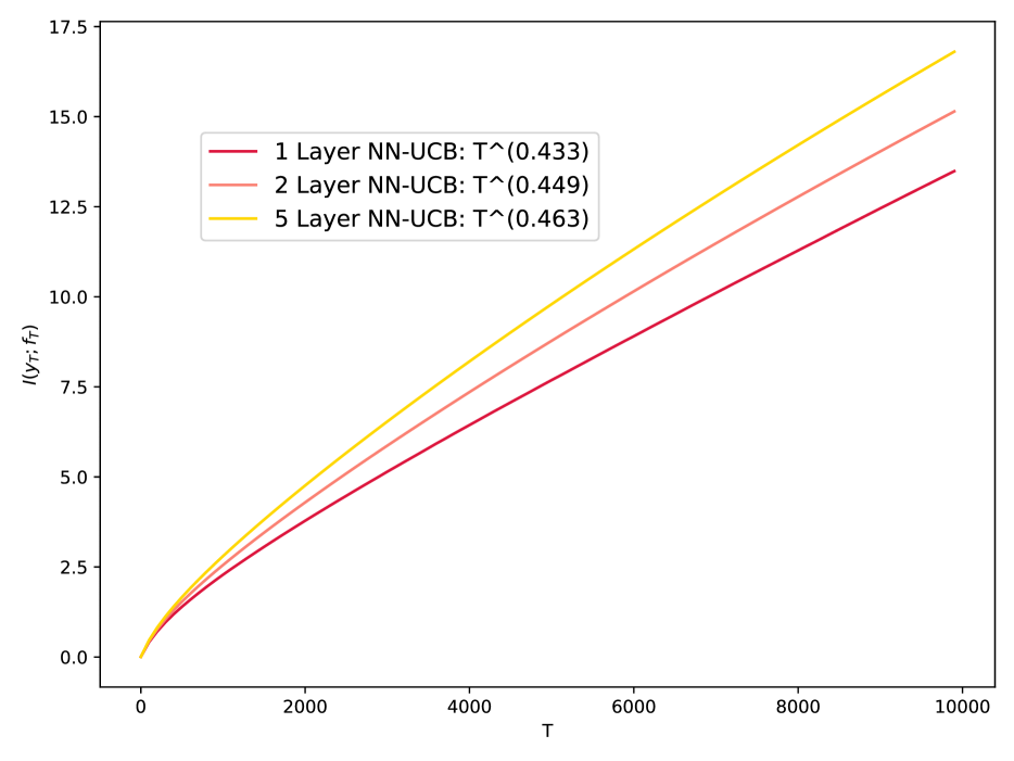
Figure 1: Empirical information gain of NN-UCB with networks of various depths, on the online MNIST classification problem, is of rate $O(T^{0.45})$. Our bound on the maximum information gain (Theorem 3.1) grows as $\tilde{\mathcal{O}}(T^{(d-1)/d})$.

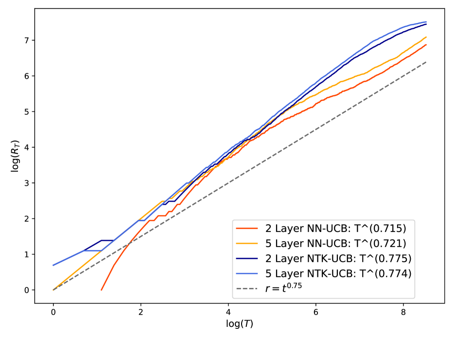
Figure 2: The regret of NTK-UCB and NN-UCB with networks of various depths, on the online MNIST classification problem, is of rate $O(T^{0.75})$. In the worst case it grows as $\tilde{\mathcal{O}}(T^{(2d-1)/2d})$ (Corollaries 3.4 & 4.4).

In Section 5, we conclude that the information gain and the regret grow with the same rate for both NTK-UCB and its convolutional variant. CNTK-UCB however, tends to have a smaller regret for every $T$. This is due to the fact that $R(T)=\tilde{\mathcal{O}}({C_{\mathrm{NN}}(d,L)}T^{(2d-1)/2d})$ for the NTK-UCB, while for the convolutional counterpart $R(T)=\tilde{\mathcal{O}}({C_{\mathrm{NN}}(d,L)}T^{(2d-1)/2d}/d^{(d-1)/2d})$ and $d\geq 1$. The upper bound on the regret being tighter for CNTK-UCB does not imply that the regret will be smaller as well. In Figure 4 we present both algorithms with the same set of contexts, and investigate whether in practice the convolutional variant can outperform NTK-UCB, which seems to be the case for the online MNIST classification task.

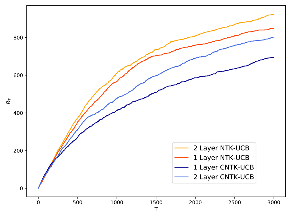
Figure 3: NN-UCB vs. CNN-UCB for online MNIST classification. Both algorithms exhibit a similar growth rate with $T$, while CNN-UCB outperforms NN-UCB, as described in Corollary 5.3.

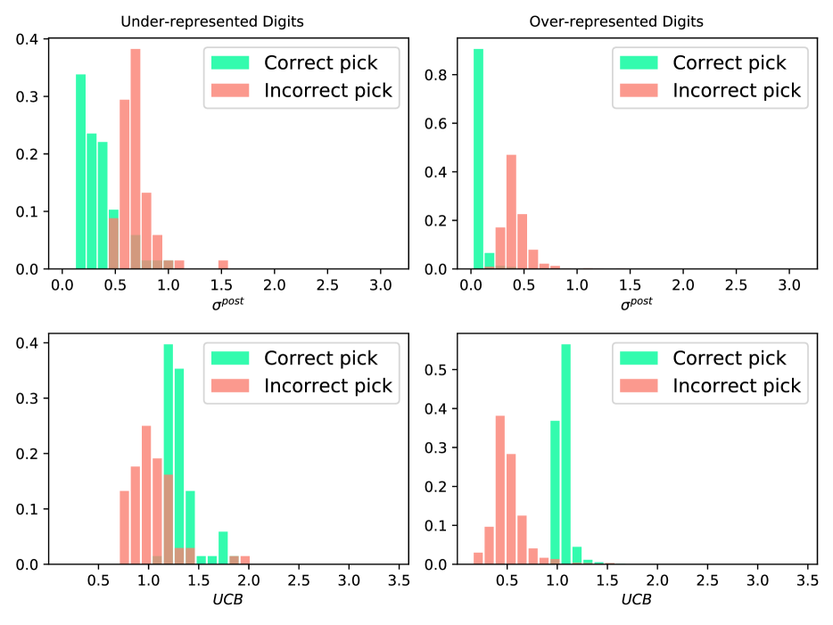
Figure 4: Under-representation Test. Histograms of $\hat{\sigma}_{t}$ and approximate UCB are plotted for an imbalanced dataset of zeros and ones. In lack of data, NN-UCB chooses the sub-optimal action with a high confidence.

A.3 NN-UCB in the face of Uncertainty

The posterior mean and variance have a transparent mathematical interpretation. For designing NN-UCB, however, we approximate $\mu_{t-1}$ and $\sigma_{t-1}$ with $f^{(J)}_{t-1}$ and $\hat{\sigma}_{t-1}$ which are not as easy to interpret. We design two experiments on MNIST to assess how well this approximation reflects the properties of the posterior mean and variance.

Effect of Imbalanced Classes

For this experiment, we limit MNIST to only zeros and ones. We create a dataset with underrepresented zeros, such that the ratio of class populations is $1:20$. This experiment shows that $\hat{\sigma}_{t-1}$ the approximate posterior variance of NN-UCB behaves as expected, similar to $\sigma_{t-1}$. The setup is as follows. Using $80\%$ of this dataset, we first run NN-UCB and train the network. On the remaining $20\%$, we continue to run the algorithm; no longer training the network, but still updating the posterior variance at every step. Presented in Figure 4, we plot the histogram of the posterior variance and upper confidence bound during the test phase. The first row presents histograms for $\sigma^{\mathrm{(post)}}({\bm{x}}_{t}^{*})$, the posterior variance calculated for the true digit ${\bm{x}}_{t}^{*}$ at step t. The lower plots show histograms of the corresponding $\mathrm{UCB}({\bm{x}}_{t}^{*})$ values. We give two separate plots for the times when the true digit ${\bm{x}}^{*}$ comes from the under-represented class, and when it comes from the over-represented class, respectively in the left and right columns. In every plot, to distinguish between the steps at which the digit picked by NN-UCB matches the true digit or not, we make a separate histogram for each case. Figure 4 demonstrates that when the ground truth is over-represented and action is picked correctly, the algorithm always has a high confidence (large UCB) and small uncertainty (posterior variance) for the true class. When the true class is over-represented, for both $\sigma^{\mathrm{post}}$ and UCB, the histogram of the steps with correct picks (green) is concentrated and well separated from the histogram of the steps with incorrect picks (red). This implies that the reason behind misclassifying an over-represented digit is having a large variance, and the algorithm is effectively performing exploration because the estimated reward is small for every action. For the under-represented class, however, the red and green histograms are not well separated. Figure 4 shows that sometimes an under-represended digit has been misclassified with a small posterior variance, or a large UCB. In lack of data, the learner is not able to refine its estimation of the posterior mean or variance. It is forced to do explorations more often which results in incorrect classifications.

Effect of Ambiguous Digits

We also assess the ability of the UCB to quantify uncertainty in light of ambiguous MNIST samples. To this end, we define an ambiguous digit to be a data point that is classified incorrectly by a well-trained classifier. We first train a $2$-layer CNN with $80\%$ of the MNIST dataset as the standard MNIST classifier. The rest of the data we use for testing. We save the misclassified digits from the test set to study NN-UCB. Figure 6 shows a few examples of such digits and the UCB for the top 5 choices of NN-UCB after observing the digit. It can be seen that for these digits there is no action which the algorithm can pick with high confidence. We first run NN-UCB on the training set. On the test set, we continue to run NN-UCB, however we do not train network any further and only update the posterior variance. For any digit, let ${\bm{x}}^{*}_{1}$ denote the maximizer of the UCB, and ${\bm{x}}^{*}_{2}$ be the class with the second largest UCB value. Figure 6 shows the histogram of $U_{{\bm{x}}^{*}_{1}}-U_{{\bm{x}}^{*}_{2}}$. The red histogram is for ambiguous samples and the green one for the non-ambiguous ones. Looking at the medians, we see that for clear samples, the algorithm often has a high confidence on its choice, while this is not the case for the ambiguous digits.

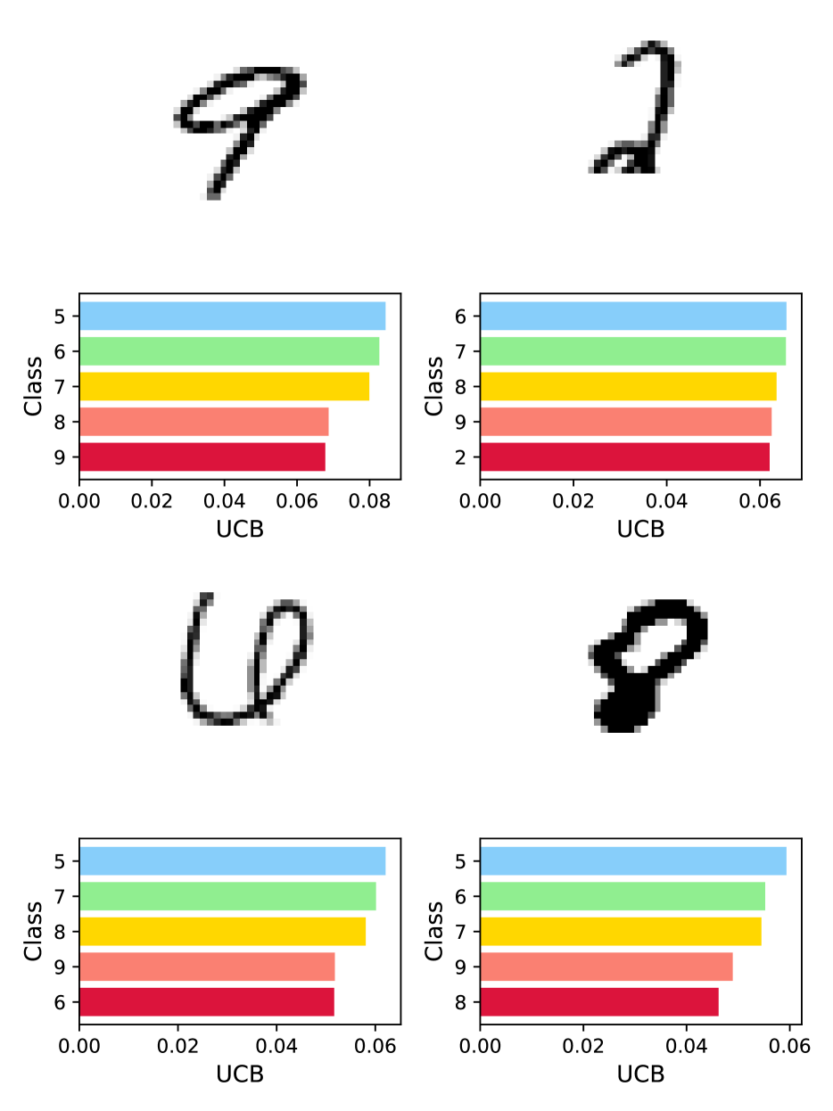
Figure 5: Examples of ambiguous Digits and the top 5 choices of NN-UCB with the largest UCBs.

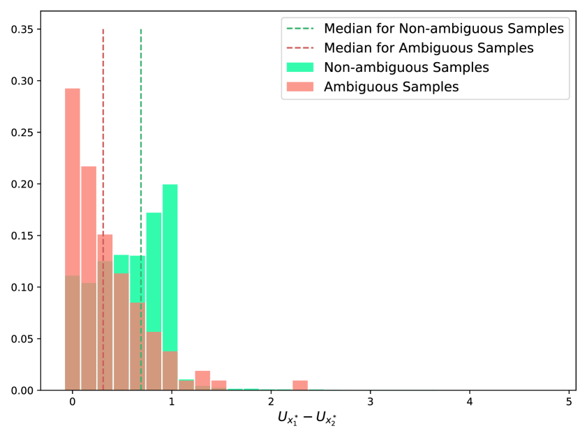
Figure 6: Ambiguity Test. Histogram of $U_{{\bm{x}}^{*}_{1}}-U_{{\bm{x}}^{*}_{2}}$ is plotted. For non-ambiguous digits, NN-UCB is significantly more confident about the class it picks.

Appendix B Details of the Main Result

Here we elaborate on a few matters from the main text.

B.1 On Section 2.1: Connections Between GP and RKHS Assumptions

We explain how the GP and RKHS assumption imposes smoothness on the reward. By assuming that $f\sim\mathrm{GP}(0,k)$, we set $\mathrm{Cov}(f({\bm{x}}),f({\bm{x}}^{\prime}))$ to $k({\bm{x}},{\bm{x}}^{\prime})$. In doing so, we enforce smoothness properties of $k$ onto $f$. As an example, suppose some normalized kernel $k$ satisfies boundedness or Lipschitz-continuity, then for $\left\lVert{\bm{x}}-{\bm{x}}^{\prime}\right\rVert\leq\delta$, $k({\bm{x}},{\bm{x}}^{\prime})$ is close to $k({\bm{x}},{\bm{x}})=1$. The GP assumption then ensures high correlation for value of $f$ at these points, making a smooth $f$ more likely to be sampled. The NTK is rotationally invariant and can be written as $\kappa({\bm{x}}^{T}{\bm{x}}^{\prime})$, where $\kappa$ is continuous and $C^{\infty}$ over $(-1,1)$, but is not differentiable at $\pm 1$ (Bietti and Bach, 2021). Therefore, our GP assumption only implies that it is more likely for $f$ to be continuous. Regarding the RKHS assumption, the Stone-Weierstrass theorem shows that any continuous function can be uniformly approximated by members of $\mathcal{H}_{k_{\mathrm{NN}}}$. We proceed by laying out the connection between the two assumptions in more detail.

Equipped with the Mercer’s theorem, we can investigate properties of $f\sim\text{GP}(0,k)$, in the general case where $k$ is a Mercer kernel and $\mathcal{X}$ is compact. The following proposition shows that sampling $f$ from a GP is equivalent to assuming $f=\sum_{i}\beta_{i}\phi_{i}$, and sampling the coefficients $\beta_{i}$ from $\mathcal{N}(0,\lambda_{i})$, where $\phi_{i}$ and $\lambda_{i}$ are the eigenfunctions and eigenvalues of the GP’s kernel function.

Proposition B.1.

Let $k$ to be a Hilbert-Schmidt continuous positive semi-definite kernel function, with $(\lambda_{i})_{i=1}^{\infty}$, and $(\phi_{i})_{i=1}^{\infty}$ indicating its eigenvalues and eigenfunctions. Assume $\mathcal{X}$ is compact. If $f\sim\text{GP}(0,k)$, then $f=\sum_{i}\beta_{i}\phi_{i}$, where $\beta_{i}\stackrel{{\scriptstyle\text{i.i.d}}}{{\sim}}\mathcal{N}(0,\lambda_{i})$.

Proof.

It suffices to show that if $f=\sum_{i}\beta_{i}\phi_{i}$, then for any ${\bm{x}},\,{\bm{x}}^{\prime}\in\mathcal{X}$, we have:

$$\mathbb{E}f({\bm{x}})=0,\quad\mathbb{E}f({\bm{x}})f({\bm{x}}^{\prime})=k({\bm{x}},{\bm{x}}^{\prime}).$$

Since $\beta_{i}$ are Gaussian and independent,

$$\mathbb{E}f({\bm{x}})=\sum_{i}\phi_{i}({\bm{x}})\,\mathbb{E}\beta_{i}=0,$$

$$\mathbb{E}f({\bm{x}})f({\bm{x}}^{\prime})=\sum_{i}\phi_{i}({\bm{x}})\phi_{i}({\bm{x}}^{\prime})\,\mathbb{E}\beta_{i}^{2}=\sum_{i}\lambda_{i}\phi_{i}({\bm{x}})\phi_{i}({\bm{x}}^{\prime})=k({\bm{x}},{\bm{x}}^{\prime}).$$

Here we have used orthonormality of $\phi_{i}$s. ∎

Proposition B.1 suggests that if $f\sim\mathrm{GP}(0,k)$ then $\left\lVert f\right\rVert_{k}$ is almost surely unbounded, since by the definition of the inner product on ${\mathcal{H}}_{k}$ we have

$$\mathbb{E}||f||_{k}^{2}=\sum_{i}\mathbb{E}\frac{\beta_{i}^{2}}{\lambda_{i}}=\sum_{i}\frac{\lambda_{i}}{\lambda_{i}}.$$

This expectation is unbounded for any kernel with an infinite number of nonzero eigenvalues. Therefore, with probability one, $||f||_{k}$ is unbounded and not a member of ${\mathcal{H}}_{k}$. However, the posterior mean of $f$ after observing $T$ samples lies in ${\mathcal{H}}_{k}$ (Proposition B.2). This connection implies that our estimate of $f$, under both RKHS and GP assumption will be a $k$-norm bounded function, similarly reflecting the smoothness properties of the kernel.

Proposition B.2.

Assume $f\sim\text{GP}(0,k)$, with $k$ Mercer and $\mathcal{X}$ compact. Then $\mu_{T}$ the posterior mean of $f$ given $({\bm{x}}_{i},y_{i})_{i=1}^{T}$ has bounded $k$-norm, and $\mu_{T}\in\mathcal{H}_{k}$.

Proof.

We first recall the Representer Theorem (Schölkopf et al., 2001). Consider the loss function $J(f)=Q({\bm{f}}_{T};{\bm{y}}_{T})+\sigma^{2}||f||_{k}$, where ${\bm{f}}_{T}=[f({\bm{x}}_{1}),\cdots,f({\bm{x}}_{T})]^{T}$. $Q$ is a $\ell_{2}$-loss assessing the fit of ${\bm{f}}_{T}$ to ${\bm{y}}_{T}$. Then $J(f)$ has a unique minimizer, which takes the form:

$$\hat{f}=\sum_{i=1}^{T}\alpha_{i}k({\bm{x}}_{i},\cdot)$$

Note that this sum is finite, hence $\hat{f}$ is $k$-norm bounded and in $\mathcal{H}_{k}$. Minimizing $J$ over $\bm{\alpha}$, we get

$$\hat{\bm{\alpha}}=(\bm{K}_{T}+\sigma^{2}\bm{I})^{-1}{\bm{y}}_{T}$$

Indicating that $\hat{f}({\bm{x}})=\mu_{T}({\bm{x}})$. ∎

B.2 On Assumptions of Theorem 4.2

For technical simplicity, in Theorem 4.2 and its convolutional extension, Theorem 5.4, we require the network at initialization to satisfy $f({\bm{x}};{\bm{\theta}}^{0})=0$ for all ${\bm{x}}\in\mathcal{X}$. We explain how this assumption can be fulfilled without limiting the problem setting to a specific network or input domain. Without loss of generality, we can initialize the network as follows. For $l\leq L$ let the weights at initialization be,

$$W^{(l)}=\begin{pmatrix}W&0\\ 0&W\end{pmatrix},\quad W^{(L+1)}=\big{(}{\bm{w}}^{T},-{\bm{w}}^{T}\big{)}$$

where entries of $W$ and ${\bm{w}}$ are i.i.d and sampled from the normal distribution. Moreover, we assume that $[{\bm{x}}]_{j}=[{\bm{x}}]_{j+d/2}$ for any ${\bm{x}}={\bm{z}}_{t}{\bm{a}}$ where $1\leq t\leq T$ and any ${\bm{a}}\in\mathcal{A}$. Any input ${\bm{x}}$ can be converted to satisfy this assumption by defining an auxiliary input $\tilde{\bm{x}}=[{\bm{x}},{\bm{x}}]/\sqrt{2}$ in a higher dimension. This mapping together with the initialization method, guarantee that output of the network at initialization is zero for every possible input that the learner may observe during a $T$-step run of the algorithm. Essentially, this property comes into effect when using result from Arora et al. (2019) or working with the Taylor expansion of the network around initialization. It allows us to write $f({\bm{x}}_{i};{\bm{\theta}})\approx\langle{\bm{g}}^{T}({\bm{x}}_{i};{\bm{\theta}}^{0}),{\bm{\theta}}-{\bm{\theta}}^{0}\rangle$.

B.3 On Section 5: CNTK as an averaged NTK

This section gives an intuition on, and serves as a sketch for proving Equation 8. Consider a 2-layer ReLU network with width $m$ defined as,

$$f_{\text{NN}}({\bm{x}};{\bm{\theta}}^{(0)})=\frac{2}{\sqrt{m}}\sum_{i=1}^{m}v_{i}^{(0)}\sigma(\langle{\bm{w}}_{i}^{(0)},{\bm{x}}\rangle)$$

where each weight parameter is an i.i.d sample from $\mathcal{N}(0,1)$. We denote the complete weight vector by ${\bm{\theta}}$ and write the first order Taylor approximation of this function with respect to ${\bm{\theta}}$ around the initialization.

$$f_{\text{NN}}({\bm{x}};{\bm{\theta}})\simeq f_{\text{NN}}({\bm{x}};{\bm{\theta}}^{(0)}) +\overbrace{\frac{2}{\sqrt{m}}\sum_{i=1}^{m}(v_{i}-v_{i}^{(0)})\sigma(\langle{\bm{w}}_{i}^{(0)},{\bm{x}}\rangle)}^{f_{\text{NN},1}({\bm{x}};{\bm{v}})}$$

$$+\underbrace{\frac{2}{\sqrt{m}}\sum_{i=1}^{m}v_{i}^{(0)}\dot{\sigma}(\langle{\bm{w}}_{i}^{(0)},{\bm{x}}\rangle)\langle{\bm{w}}_{i}-{\bm{w}}_{i}^{(0)},{\bm{x}}\rangle}_{f_{\text{NN},2}({\bm{x}};{\bm{W}})}$$

We limit the input domain to ${\mathbb{S}}^{d-1}$, equipped with the uniform measure. Consider the function class $\mathcal{F}_{\text{NTK}}=\{f({\bm{x}})=f_{\text{NN},1}({\bm{x}};{\bm{v}})+f_{\text{NN},2}({\bm{x}};{\bm{W}})\,\text{ s.t. }\,{\bm{v}}\in{\mathbb{R}}^{m},\,{\bm{W}}\in{\mathbb{R}}^{m\times d}\}$. It is straightforward to show that $\mathcal{F}_{\text{NTK}}$ is an RKHS and the following kernel function satisfies the reproducing property for ${\mathcal{F}}_{\text{NTK}}$ (Chizat et al., 2019).

$$h({\bm{x}},{\bm{x}}^{\prime})=\frac{1}{m}\sum_{i=1}^{m}\sigma(\langle{\bm{w}}_{i}^{(0)},{\bm{x}}\rangle)\sigma(\langle{\bm{w}}_{i}^{(0)},{\bm{x}}^{\prime}\rangle)+\frac{1}{m}\sum_{i=1}^{m}{\bm{x}}^{T}{\bm{x}}^{\prime}(v_{i}^{(0)})^{2}\dot{\sigma}(\langle{\bm{w}}_{i}^{(0)},{\bm{x}}\rangle)\dot{\sigma}(\langle{\bm{w}}_{i}^{(0)},{\bm{x}}^{\prime}\rangle)$$

Random Feature Derivation of 2-layer CNTK

We repeat the first order Taylor approximation for $f_{\text{CNN}}$.

$$f_{\text{CNN}}({\bm{x}};{\bm{\theta}})\simeq f_{\text{CNN}}({\bm{x}};{\bm{\theta}}^{(0)}) +\overbrace{\frac{2}{\sqrt{m}}\sum_{i=1}^{m}(v_{i}-v_{i}^{(0)})\big{[}\frac{1}{d}\sum_{l=1}^{d}\sigma(\langle{\bm{w}}_{i}^{(0)},c_{l}\cdot{\bm{x}}\rangle)\big{]}}^{f_{\text{CNN,}1}({\bm{x}};{\bm{v}})}$$

$$+\underbrace{\frac{2}{\sqrt{m}}\sum_{i=1}^{m}v_{i}^{(0)}\big{[}\frac{1}{d}\sum_{l=1}^{d}\dot{\sigma}(\langle{\bm{w}}_{i}^{(0)},c_{l}\cdot{\bm{x}}\rangle)\langle{\bm{w}}_{i}-{\bm{w}}_{i}^{(0)},c_{l}\cdot{\bm{x}}\rangle\big{]}}_{f_{\text{CNN,}2}({\bm{x}};{\bm{W}})}$$

And define $\mathcal{F}_{\text{CNTK}}$ to be the convolutional counterpart of $\mathcal{F}_{\text{NTK}}$

$$\mathcal{F}_{\text{CNTK}}=\{f({\bm{x}})=f_{\text{CNN,}1}({\bm{x}};{\bm{v}})+f_{\text{CNN,}2}({\bm{x}};{\bm{W}})\,\text{ s.t. }\,{\bm{v}}\in{\mathbb{R}}^{m},\,{\bm{W}}\in{\mathbb{R}}^{m\times d}\}.$$

Then $\mathcal{F}_{\text{CNTK}}$ is reproducing for the following kernel function,

$$\bar{h}({\bm{x}},{\bm{x}}^{\prime}) =\frac{1}{m}\sum_{i=1}^{m}\frac{1}{d^{2}}\sum_{l=1}^{d}\sum_{l^{\prime}=1}^{d}\sigma(\langle{\bm{w}}_{i}^{(0)},c_{l}\cdot{\bm{x}}\rangle)\sigma(\langle{\bm{w}}_{i}^{(0)},c_{l^{\prime}}\cdot{\bm{x}}^{\prime}\rangle)$$

$$\quad+\frac{1}{m}\sum_{i=1}^{m}\frac{1}{d^{2}}\sum_{l=1}^{d}\sum_{l^{\prime}=1}^{d}\langle c_{l}\cdot{\bm{x}},c_{l^{\prime}}\cdot{\bm{x}}^{\prime}\rangle(v_{i}^{(0)})^{2}\dot{\sigma}(\langle{\bm{w}}_{i}^{(0)},c_{l}\cdot{\bm{x}}\rangle)\dot{\sigma}(\langle{\bm{w}}_{i}^{(0)},c_{l^{\prime}}\cdot{\bm{x}}^{\prime}\rangle)$$

As $m$ the number of channels grows, the average over the parameters converges to the expectation over ${\bm{w}}$ and ${\bm{v}}$, and the kernel becomes rotation invariant, i.e. only depends on the angle between ${\bm{x}}$ and ${\bm{x}}^{\prime}$.

$$\lim_{m\rightarrow\infty}\bar{h}({\bm{x}},{\bm{x}}^{\prime}) =\lim_{m\rightarrow\infty}\frac{1}{d}\frac{1}{m}\sum_{i=1}^{m}\sum_{l=1}^{d}\sigma(\langle{\bm{w}}_{i}^{(0)},c_{l}\cdot{\bm{x}}\rangle)\sigma(\langle{\bm{w}}_{i}^{(0)},{\bm{x}}^{\prime}\rangle)$$

$$\qquad\quad+\langle c_{l}\cdot{\bm{x}},{\bm{x}}^{\prime}\rangle(v_{i}^{(0)})^{2}\dot{\sigma}(\langle{\bm{w}}_{i}^{(0)},c_{l}\cdot{\bm{x}}\rangle)\dot{\sigma}(\langle{\bm{w}}_{i}^{(0)},{\bm{x}}^{\prime}\rangle)$$

$$=\frac{1}{d}\sum_{l=1}^{d}h(c_{l}\cdot{\bm{x}},{\bm{x}}^{\prime})$$

Equation 8 follows by noting that in the infinite $m$ limit, $h$ and $\bar{h}$ converge to ${k_{\mathrm{NN}}}$ and ${k_{\mathrm{CNN}}}$ respectively. A rigorous proof is given in Propostition 4 from Mei et al. (2021).

B.4 Proof of Lemma 5.1

Let $V_{d,k}$ be the space of degree-$k$ polynomials that are orthogonal to the space of polynomials of degree less than $k$, defined on ${\mathbb{S}}^{d-1}$. Then $V_{d,k}({\mathcal{C}}_{d})$ denotes the subspace of $V_{d,k}$ that is also ${\mathcal{C}}_{d}$-invariant.

Proof of Lemma 5.1.

The NTK kernel satisfies the Mercer condition and has the following Mercer decomposition (Bietti and Bach, 2021),

$$k_{\text{NTK}}({\bm{x}},{\bm{x}}^{\prime})=\sum_{k=0}^{\infty}\mu_{k}\sum_{j=1}^{N(d,k)}Y_{j,k}({\bm{x}})Y_{j,k}({\bm{x}}^{\prime})$$

where $\{Y_{j,k}\}_{j\leq N(d,k)}$ form an orthonormal basis for $V_{d,k}$. Bietti and Bach (2021) further show that $Y_{j,k}$ is the $j$-th spherical harmonic polynomial of degree $k$, and $N(d,k)=\text{dim}(V_{d,k})$ gives the total count of such polynomials, where

$$N(d,k)=\frac{2k+d-2}{k}\binom{k+d-3}{d-2}.$$

For any integer $k$, it also holds that (Bietti and Bach, 2021)

$$\sum_{j=1}^{N(d,k)}Y_{j,k}({\bm{x}})Y_{j,k}({\bm{x}}^{\prime})=N(d,k)Q^{(d)}_{k}({\bm{x}}^{T}{\bm{x}}^{\prime})$$ (B.1)

where $Q_{k}^{(d)}$ is the $k$-th Gegenbauer polynomial in dimension $d$. It follows from Equation 8 that $k_{\text{CNTK}}$ is also Mercer. Assume that it has a Mercer decomposition of the form

$$k_{\text{CNTK}}({\bm{x}},{\bm{x}}^{\prime})=\sum_{k=0}^{\infty}\bar{\mu}_{k}\sum_{j=1}^{\bar{N}(d,k)}\bar{Y}_{j,k}({\bm{x}})\bar{Y}_{j,k}({\bm{x}}^{\prime}).$$

We now proceed to identify $\bar{Y}_{j,k}$ and calculate $\bar{N}(d,k)$. From Equations 8 and B.1 we conclude that

$$\bar{k}({\bm{x}},{\bm{x}}^{\prime})=\frac{1}{d}\sum_{l=1}^{d}k({\bm{x}},c_{l}\cdot{\bm{x}}^{\prime})=\frac{1}{d}\sum_{l=1}^{d}\sum_{k=0}^{\infty}\mu_{k}N(d,k)Q^{(d)}_{k}(\langle{\bm{x}},c_{l}\cdot{\bm{x}}^{\prime}\rangle).$$

Lemma 1 in Mei et al. (2021) states that for any integer $k$,

$$\frac{1}{d}N(d,k)\sum_{l=1}^{d}Q_{k}^{(d)}(\langle{\bm{x}},c_{l}\cdot{\bm{x}}^{\prime}\rangle)=\sum_{j=1}^{M(d,k)}Z_{j,k}({\bm{x}})Z_{j,k}({\bm{x}}^{\prime})$$ (B.2)

where $Z_{j,k}$ form an orthonormal basis for $V_{d,k}({\mathcal{C}}_{d})$. Moreover, for the orthonormal basis $(Z_{j,k})_{j}$ over ${\mathbb{S}}^{d-1}$,

$$\sum_{j=1}^{M(d,k)}Z_{j,k}({\bm{x}})Z_{j,k}({\bm{x}})=M(d,k).$$ (B.3)

Therefore, $(\mu_{k},Z_{j,k})_{j,k}$ is a sequence eigenvalue eigenfunction pairs for $\bar{k}$ and the following assignments satisfy the Mercer decomposition for $k_{\text{CNTK}}$:

$$\bar{\mu}_{k} =\mu_{k},$$

$$\bar{Y}_{j,k} =Z_{j,k},$$

$$\bar{N}(d,k) =M(d,k).$$

It remains to show that $M(d,k)\simeq N(d,k)/d$ when $C_{d}$ is the group of cyclic shifts acting on ${\mathbb{S}}^{d-1}$. This follows from Equations B.2 and B.3,

$$\frac{M(d,k)}{N(d,k)} =\frac{1}{d}\sum_{l=1}^{d}Q_{k}^{(d)}(\langle{\bm{x}},c_{l}\cdot{\bm{x}}\rangle)$$

$$=\Theta(d^{-1})$$

where the last equation holds directly due to Lemma 4 in Mei et al. (2021). ∎

Appendix C Details of NTK-UCB and CNTK-UCB

Section C.1 gives the proof to our statement on the information gain (Theorem 3.1, Proposition 5.2). The regret bounds of NTK-UCB under the GP (Theorem 3.2) and the RKHS assumptions (Theorem 3.3) are proven in Section C.2 and Section C.4, respectively. In Section C.3, we present SupNTK-UCB (Algorithm 2), and discuss the exploration policy of this algorithm and its properties.

C.1 Proof of Theorem 3.1 and Proposition 5.2

We begin by giving an overview of the proof. Under the conditions of Theorem 3.1, the NTK is Mercer (Cao et al., 2021) and can be written as $k({\bm{x}},{\bm{x}}^{\prime})=\sum_{i\geq 0}\lambda_{i}\phi_{i}({\bm{x}})\phi_{i}({\bm{x}}^{\prime})$, with $(\phi_{i})_{i\geq 0}$ denoting the orthonoromal eigenfunctions. The main idea is to break $k$ into $k_{p}+k_{o}$ where $k_{p}({\bm{x}},{\bm{x}}^{\prime})=\sum_{i\leq\tilde{D}}\lambda_{i}\phi_{i}({\bm{x}})\phi_{i}({\bm{x}}^{\prime})$ has a finite dimensional feature map $(\phi_{i})_{i\leq\tilde{D}}$, corresponding to the sequence of $\tilde{D}$ largest eigenvalues of $k$. For any arbitrary sequence $X_{T}$, we are then able to decompose $I({\bm{y}}_{T};{\bm{f}}_{T})$ in two terms, one corresponding to information gain of $k_{p}$, and the other, the tail sum of the eigenvalue series $\sum_{i\geq\tilde{D}}\lambda_{i}$. We proceed by bounding each term separately and picking $\tilde{D}$ such that the second term becomes negligible.

Proof of Theorem 3.1.

This proof adapts the finite-dimensional projection idea used in Vakili et al. (2021a). Cao et al. (2021) show that the NTK has a Mercer decomposition on the $d$-dimensional unit hyper-sphere. Bietti and Bach (2021) establish that

$${k_{\mathrm{NN}}}({\bm{x}},{\bm{x}}^{\prime})=\sum_{k\geq 0}\mu_{k}\sum_{j=1}^{N(d,k)}Y_{j,k}({\bm{x}})Y_{j,k}({\bm{x}}^{\prime}),$$

where $Y_{j,k}$ is the $j$-th spherical harmonic polynomial of degree $k$, and for $k\geq 1$ there are

$$N(d,k)=\frac{2k+d-2}{k}\binom{k+d-3}{d-2}$$

of such $k$-degree polynomials. Using Stirling’s approximation we can show that $N(d,k)=\Theta(k^{d-2})$. The functions $\{Y_{j,k}\}$ are an algebraic basis for $\mathcal{H}_{k_{\mathrm{NN}}}$ the RKHS that is reproducing for ${k_{\mathrm{NN}}}$. Consider a finite dimensional subspace of $\mathcal{H}_{k_{\mathrm{NN}}}$ that is spanned by the eigenfunctions corresponding to the first $D$ distinct eigenvalues of ${k_{\mathrm{NN}}}$, ${\bm{\phi}}_{D}=\left((Y_{j,0})_{j\leq N(d,0)},\cdots,(Y_{j,D})_{j\leq N(d,D)}\right)$. We decompose the NTK as ${k_{\mathrm{NN}}}=k_{P}+k_{O}$, where $k_{P}$ is the kernel for the finite dimensional RKHS, and $k_{O}$ represents the kernel for the Hilbert space orthogonal to it. Let $\tilde{D}$ denote the length of ${\bm{\phi}}_{D}$, the feature map corresponding to $k_{P}$,

$$D\leq\tilde{D}=\sum_{k=0}^{D}N(d,k)\simeq C\sum_{k=0}^{D}k^{d-2}\leq C\frac{(D+1)^{d-1}}{d-1}.$$ (C.1)

Note that the first $\tilde{D}$ eigenvalues of ${k_{\mathrm{NN}}}$ make up its first $D$ distinct eigenvalues. We write the information gain in terms of eigenvalues of $k_{p}$ and $k_{O}$, and find $D$ such that the finite-dimensional term dominates the infinite-dimensional tail. Assume the arbitrary sequence $X_{T}=({\bm{x}}_{1},\cdots,{\bm{x}}_{T})$ is observed. The information gain is $I({\bm{y}}_{T};{\bm{f}}_{T})=\frac{1}{2}\log\det({\bm{I}}+\sigma^{-2}K_{X_{T}})$, with $K_{X_{T}}$ being the kernel matrix, $(K_{X_{T}})_{i,j}={k_{\mathrm{NN}}}({\bm{x}}_{i},{\bm{x}}_{j})$. Using a similar notation for the kernel matrices of $k_{P}$ and $k_{O}$, we may write

$$\begin{split}I({\bm{y}}_{T};{\bm{f}}_{T})&=\frac{1}{2}\log\det({\bm{I}}+\sigma^{-2}(K_{P,X_{T}}+K_{O,X_{T}}))\\ &=\frac{1}{2}\log\det({\bm{I}}+\sigma^{-2}K_{P,X_{T}})+\frac{1}{2}\log\det({\bm{I}}+({\bm{I}}+\sigma^{-2}K_{P,X_{T}})^{-1}K_{O,X_{T}})\\ \end{split}$$ (C.2)

We now separately bound the two terms. Let $\bm{\Phi}_{D,T}=[{\bm{\phi}}_{D}({\bm{x}}_{1}),\cdots,{\bm{\phi}}_{D}({\bm{x}}_{T})]^{T}$, then by the mercer decomposition,

$$K_{P,X_{T}}=\bm{\Phi}_{D,T}\Lambda_{D}\bm{\Phi}_{D,T}^{T}$$

Where $\Lambda_{D}\in{\mathbb{R}}^{\tilde{D}\times\tilde{D}}$ is a diagonal matrix with the first $\tilde{D}$ eigenvalues. Let ${\bm{H}}_{T}=\Lambda^{1/2}_{D}\bm{\Phi}^{T}_{D,T}\bm{\Phi}_{D,T}\Lambda_{D}^{1/2}$, by Weinstein-Aronszajn identity,

$$\begin{split}\frac{1}{2}\log\det({\bm{I}}_{T}+\sigma^{-2}K_{P,X_{T}})&=\frac{1}{2}\log\det({\bm{I}}+\sigma^{-2}{\bm{H}}_{T})\\ &\leq\frac{1}{2}\tilde{D}\log\left(\text{tr}({\bm{I}}+\sigma^{-2}{\bm{H}}_{T})/\tilde{D}\right)\end{split}$$

For positive definite matrices ${\bm{P}}\in\mathbb{R}^{n\times n}$, we have $\log\det{\bm{P}}\leq n\log\text{tr}({\bm{P}}/n)$. The inequality follows from ${\bm{I}}_{D}+\sigma^{-2}{\bm{H}}_{T}$ being positive definite. Plugging in the definition of ${\bm{H}}_{T}$

$$\begin{split}\frac{1}{2}\log\det({\bm{I}}_{T}+\sigma^{-2}K_{P,X_{T}})&\leq\frac{1}{2}\tilde{D}\log\left(1+\frac{\sigma^{-2}}{\tilde{D}}\text{tr}\left(\Lambda^{1/2}_{D}\bm{\Phi}^{T}_{D,T}\bm{\Phi}_{D,T}\Lambda_{D}^{1/2}\right)\right)\\ &\leq\frac{1}{2}\tilde{D}\log\left(1+\frac{\sigma^{-2}}{\tilde{D}}\sum_{t=1}^{T}\Lambda^{1/2}_{D}\Phi^{T}_{D}({\bm{x}}_{t}){\bm{\phi}}_{D}({\bm{x}}_{t})\Lambda_{D}^{1/2}\right)\\ &\leq\frac{1}{2}\tilde{D}\log\left(1+\frac{\sigma^{-2}}{\tilde{D}}\sum_{t=1}^{T}||{\bm{\phi}}_{D}({{\bm{x}}_{t}})\Lambda^{1/2}||_{2}^{2}\right)\\ &\leq\frac{1}{2}\tilde{D}\log\left(1+\frac{\sigma^{-2}}{D}\sum_{t=1}^{T}\sum_{k=0}^{D}\mu_{k}\sum_{j=1}^{N(d,k)}Y_{j,k}^{2}({\bm{x}}_{t})\right)\\ &\leq\frac{1}{2}\tilde{D}\log\left(1+\frac{\sigma^{-2}}{\tilde{D}}\sum_{t=1}^{T}k_{P}({\bm{x}}_{t},{\bm{x}}_{t})\right)\\ &\leq\frac{1}{2}\tilde{D}\log\left(1+\frac{\sigma^{-2}T}{\tilde{D}}\right)\end{split}$$

The last inequality holds since the NTK is uniformly bounded by $1$ on the unit sphere. We now bound the second term in Equation C.2, which corresponds to the infinite-dimensional orthogonal space. Similar to the first term, we bound $\log\det{\bm{P}}$ with $n\log\text{tr}({\bm{P}}/n)$,

$$\begin{split}\frac{1}{2}\log\det({\bm{I}}_{T}+({\bm{I}}_{T}+\sigma^{-2}K_{P,X_{T}})^{-1}K_{O,X_{T}})&\leq\frac{T}{2}\log\left(1+\frac{\text{tr}\left(({\bm{I}}_{T}+\sigma^{-2}K_{P,X_{T}})^{-1}K_{O,X_{T}}\right)}{T}\right)\\ &\leq\frac{T}{2}\log\left(1+\text{tr}\left(K_{O,X_{T}}\right)/T\right)\end{split}$$ (C.3)

The second inequality holds due to $({\bm{I}}_{T}+\sigma^{-2}K_{P,X_{T}})^{-1}$ being positive definite, with eigenvalues smaller than $1$. We can bound the trace using the Mercer decomposition

$$\begin{split}\text{tr}\left(K_{O,X_{T}}\right)&=\sum_{t=1}^{T}k_{O}({\bm{x}}_{t},{\bm{x}}_{t})\\ &=\sum_{t=1}^{T}\sum_{k=D+1}^{\infty}\mu_{k}\sum_{j=1}^{N(d,k)}Y_{j,k}^{2}({\bm{x}}_{t})\\ &=\sum_{t=1}^{T}\sum_{k=D+1}^{\infty}\mu_{k}N(d,k)Q^{(d)}_{k}({\bm{x}}_{t}^{T}{\bm{x}}_{t})\end{split}$$

where $Q^{(d)}_{k}$ is the Gegenbauer polynomial of degree $k$ and ${\bm{x}}_{t}$ are on ${\mathbb{S}}^{d-1}$. We have $Q^{(d)}_{K}(1)=1$ which gives,

$$\text{tr}\left(K_{O,X_{T}}\right)=T\sum_{k=D+1}^{\infty}\mu_{k}N(d,k)$$ (C.4)

Plugging in Equation C.4 in Equation C.3, the information gain can be bounded as,

$$I({\bm{y}}_{T},{\bm{f}}_{T})\leq\frac{\tilde{D}}{2}\log\left(1+\frac{T}{\sigma^{2}\tilde{D}}\right)+\frac{T}{2}\log\left(1+\sum_{k=D+1}^{\infty}\mu_{k}N(d,k)\right)$$

We now bound the second term using Bietti and Bach’s result on decay rate of $\mu_{k}$. They show that there exists a constant $C_{1}(d,L)$ such that $\mu_{k}\leq C_{1}k^{-d}$. Using Stirling approximation, there exists $C_{2}$ such that $N(d,k)\leq C_{2}k^{d-2}$. Then,

$$\sum_{k=D+1}^{\infty}\mu_{k}N(d,k)\leq C(d,L)\sum_{k=D+1}^{\infty}k^{-2}$$

We can simply bound the series

$$\sum_{k=D+1}^{\infty}k^{-2}\leq\int_{D}^{\infty}z^{-2}dz=\frac{1}{D}.$$

Therefore, there exists there exists ${C(d,L)}$ such that,

$$\begin{split}I({\bm{y}}_{T},{\bm{f}}_{T})&\leq\frac{\tilde{D}}{2}\log\left(1+\frac{T}{\sigma^{2}\tilde{D}}\right)+\frac{T}{2}\log\left(1+\frac{{C(d,L)}}{D}\right)\\ &\leq\frac{\tilde{D}}{2}\log\left(1+\frac{T}{\sigma^{2}\tilde{D}}\right)+\frac{T{C(d,L)}}{2D}\end{split}$$ (C.5)

Note that the first term is increasing with $\tilde{D}$. We pick $\tilde{D}$ such that the first term in Equation C.5 is dominant. Via Equation C.1 we set,

$$\tilde{D}=\Big{\lceil}\left(\frac{{C(d,L)}T}{\log(1+\sigma^{-2}T)}\right)^{\frac{d-1}{d}}\Big{\rceil}$$

The treatment above holds for any arbitrary sequence $X_{T}$. Plugging in $\tilde{D}$ with Equation C.5, we then may write,

$$\gamma_{T}\leq\left(\frac{{C(d,L)}T}{\log(1+\sigma^{-2}T)}\right)^{\frac{d-1}{d}}\log\left(1+\sigma^{-2}T\left(\frac{{C(d,L)}T}{\log(1+\sigma^{-2}T)}\right)^{\frac{d}{d-1}}\right)$$

which concludes the proof. ∎

Proof of Proposition 5.2.

The CNTK is Mercer by Lemma 5.1. Which implies that we may repeat the steps taken in the proof of Theorem 3.1. To avoid confusion, we use the “bar” notation to indicate the convolutional equivalent of the parameters from that proof. The 2-layer CNTK and the NTK share the same eigenvalues. The eigenfunctions of the CNTK also bounded by one over the hyper sphere. The only difference is that $\bar{N}(d,k)=N(d,k)/d$, which comes into effect for calculating $\text{tr}(\bar{K}_{O,X_{T}})$. For the CNTK we would have,

$$\text{tr}\left(\bar{K}_{O,X_{T}}\right)=T\sum_{k=\bar{D}+1}^{\infty}\mu_{k}\bar{N}(d,k)=T\sum_{k=\bar{D}+1}^{\infty}\mu_{k}N(d,k)/d$$

Equivalent to Equation C.5 we may write,

$$\bar{I}({\bm{y}}_{T},{\bm{f}}_{T})\leq\frac{\tilde{D}}{2}\log\left(1+\frac{T}{\sigma^{2}\tilde{D}}\right)+\frac{T{C(d,L)}}{2\bar{D}d}$$

where similar to the proof of Theorem 3.1, we have $\tilde{D}=\Theta(\bar{D}^{d-1})$. For the first term to be larger than the second, $\tilde{D}$ has to be set to

$$\tilde{D}=\Big{\lceil}\left(\frac{{C(d,L)}T}{d\log(1+\sigma^{-2}T)}\right)^{\frac{d-1}{d}}\Big{\rceil}$$

which then concludes the proof. ∎

C.2 Proof of Theorem 3.2

The proof closely follows the method in Srinivas et al. (2010) and Krause and Ong (2011), with modifications on the assumptions on context domain and actions. The following lemmas will be used.

Lemma C.1.

Let $\delta\in(0,1)$, and set $\beta_{t}=2\log(|\mathcal{A}|\pi_{t}/\delta)$, where $\sum_{t>1}\pi_{t}^{-1}=1$ and $\pi_{t}>0$. Then with probability of at least $1-\delta$

$$|f({\bm{z}}_{t}{\bm{a}})-\mu_{t-1}({\bm{z}}_{t}{\bm{a}})|\leq\sqrt{\beta_{t}}\sigma_{t-1}({\bm{z}}_{t}{\bm{a}}),\quad\forall{\bm{a}}\in\mathcal{A},\,\forall t>1.$$

Lemma C.2.

Let $\sigma_{t-1}^{2}({\bm{x}}_{t})$ be the posterior variance, computed at ${\bm{x}}_{t}={\bm{z}}_{t}{\bm{a}}_{t}$, where ${\bm{a}}_{t}$ is the action picked by the UCB policy. Then,

$$\frac{1}{2}\sum_{t=1}^{T}\log(1+\sigma^{-2}\sigma_{t-1}^{2}({\bm{x}}_{t}))\leq\gamma_{T}$$

Proof of Theorem 3.2.

We use Lemma C.1, to bound the regret at step $t$. Let ${\bm{x}}_{t}^{*}={\bm{z}}_{t}{\bm{a}}^{*}$ denote the optimal point, and ${\bm{x}}_{t}={\bm{z}}_{t}{\bm{a}}_{t}$ be the maximizer of the UCB. Then by Lemma C.1, with probability of at least $1-\delta$

$$\begin{split}&|f({\bm{x}}_{t})-\mu_{t-1}({\bm{x}}_{t})|\leq\sqrt{\beta_{t}}\sigma_{t-1}({\bm{x}}_{t})\\ &|f({\bm{x}}_{t}^{*})-\mu_{t-1}({\bm{x}}_{t}^{*})|\leq\sqrt{\beta_{t}}\sigma_{t-1}({\bm{x}}_{t}^{*})\end{split}$$

Therefore, by definition of ${\bm{x}}_{t}$ (Equation 5) we can write:

$$\begin{split}r_{t}=f({\bm{x}}_{t}^{*})-f({\bm{x}}_{t})&\leq\mu_{t-1}({\bm{x}}_{t}^{*})+\sqrt{\beta_{t}}\sigma_{t-1}({\bm{x}}_{t}^{*})-f({\bm{x}}_{t})\\ &\leq\mu_{t-1}({\bm{x}}_{t})+\sqrt{\beta_{t}}\sigma_{t-1}({\bm{x}}_{t})-f({\bm{x}}_{t})\\ &\leq 2\sqrt{\beta_{t}}\sigma_{t-1}({\bm{x}}_{t}).\end{split}$$

For the regret over $T$ steps, by Cauchy-Schwartz we have,

$$\begin{split}R_{T}=\sqrt{\sum_{t=1}^{T}r_{t}}&\leq\sqrt{T}\sqrt{\sum_{t=1}^{T}r_{t}^{2}}\\ &\leq\sqrt{T}\sqrt{\sum_{t=1}^{T}4\beta_{t}\sigma_{t-1}^{2}({\bm{x}}_{t})}.\end{split}$$ (C.6)

Recall that Lemma C.1, holds for any $\beta_{t}=2\log(|\mathcal{A}|\pi_{t}/\delta)$, where $\sum_{t>1}\pi_{t}^{-1}=1$. We pick $\pi_{t}=\frac{\pi^{2}t^{2}}{6}$, so that $\beta_{t}$ is non-increasing and can be upper bounded by $\beta_{T}$. This allows to reduce the problem of bounding regret to the bounding the sum of posterior variances. By Equation 4, and since ${k_{\mathrm{NN}}}({\bm{x}},{\bm{x}})\leq 1$,

$$\sigma^{-2}\sigma_{t-1}^{2}({\bm{x}}_{t})\leq\sigma^{-2}{k_{\mathrm{NN}}}({\bm{x}}_{t},{\bm{x}}_{t})\leq\sigma^{-2}$$

For any $r\in[0,a]$, it holds that $r\leq\frac{a\log(1+r)}{\log(1+a)}$. Therefore,

$$\sigma^{-2}\sigma_{t-1}^{2}\leq\frac{\sigma^{-2}}{\log(1+\sigma^{-2})}\log(1+\sigma^{-2}\sigma_{t-1}^{2})$$

Putting together the sum in Equation C.6 we get,

$$\begin{split}R_{t}&\leq\sqrt{4T\beta_{T}\sigma^{2}{\sum_{t=1}^{T}}\sigma^{-2}\sigma_{t-1}^{2}}\\ &\leq\sqrt{\frac{4T\beta_{T}\sigma^{2}}{\log(1+\sigma^{-2})}\sum_{t=1}^{T}\log(1+\sigma^{-2}\sigma_{t-1}^{2})}\\ &\leq\sqrt{\frac{8\sigma^{2}}{\log(1+\sigma^{-2})}}\sqrt{T\beta_{T}\gamma_{T}}\end{split}$$

where the last inequality holds by plugging in Lemma C.2. ∎

C.2.1 Proof of Lemma C.1

Proof.

Fix $t\geq 1$. Conditioned on ${\bm{y}}_{t-1}=(y_{1},\cdots,y_{t-1})$, ${\bm{x}}_{1},\cdots,{\bm{x}}_{t-1}$ are deterministic. The posterior distribution is $f({\bm{x}})\sim N(\mu_{t-1}({\bm{x}}),\sigma^{2}_{t-1}({\bm{x}}))$. Applying the sub-Gaussian inequality, and conditioned on the history,

$$\text{Pr}[|f({\bm{x}})-\mu_{t-1}({\bm{x}})|>\sqrt{\beta_{t}}\sigma_{t-1}({\bm{x}})]\leq e^{-\beta_{t}/2}$$

$\mathcal{A}$ is finite and ${\bm{x}}={\bm{z}}_{t}{\bm{a}}$, then by union bound over $S$, the following holds with probability of at least $1-|\mathcal{A}|e^{-\beta_{t}/2}$,

$$|f({\bm{z}}_{t}{\bm{a}})-\mu_{t-1}({\bm{z}}_{t}{\bm{a}})|\leq\sqrt{\beta_{t}}\sigma_{t-1}({\bm{z}}_{t}{\bm{a}}),\quad\forall{\bm{a}}\in\mathcal{A}$$

It is only left to further apply a union bound over all $t\geq 1$. For the statement in lemma to hold, $\beta_{t}$ has to be set such that, $\sum_{t\geq 1}|\mathcal{A}|e^{\beta_{t}/2}\leq\delta$. Setting $\beta_{t}=2\log(|\mathcal{A}|\pi_{t}/\delta)$ with $\sum_{t>1}\pi_{t}=1$ satisfies the condition. ∎

C.2.2 Proof of Lemma C.2

Proof.

Recall that for a Gaussian random variable entropy is, $H(N(\bm{\mu,\Sigma}))=\frac{1}{2}\log\det(2\pi e\bm{\Sigma)}$. Let ${\bm{y}}_{T}$ be the vector of observed rewards and ${\bm{f}}_{T}=[f({\bm{x}}_{t})]_{t\leq T}\in\mathbb{R}^{T}$ the true rewards. We have ${\bm{y}}_{T}={\bm{f}}_{T}+\bm{\epsilon}_{T}$, therefore, ${\bm{y}}_{T}|{\bm{f}}_{T}\sim N(0,\bm{I}\sigma^{2})$, and $y_{T}|{\bm{y}}_{T-1}\sim N(\mu_{T-1},\sigma^{2}+\sigma_{T-1}^{2}({\bm{x}}_{T})))$. By the definition of mutual information,

$$\begin{split}I({\bm{y}}_{T};{\bm{f}}_{T})&=H({\bm{y}}_{T})-H({\bm{y}}_{T}|{\bm{f}}_{T})\\ &=H({\bm{y}}_{T-1})+H(y_{T}|{\bm{y}}_{T-1})-\frac{T}{2}\log(2\pi e\sigma^{2})\\ &=H({\bm{y}}_{T-1})+\frac{1}{2}\log(2\pi e(\sigma^{2}+\sigma_{T-1}^{2}({\bm{x}}_{T})))-\frac{T}{2}\log(2\pi e\sigma^{2}).\\ \end{split}$$

The first equality holds by the chain rule for entropy. By recursion,

$$\gamma_{T}\geq I({\bm{y}}_{T};{\bm{f}}_{T})=\frac{1}{2}\sum_{t=1}^{T}\log(1+\sigma^{-2}\sigma_{t-1}^{2}({\bm{x}}_{t}))$$

∎

C.3 The Sup Variant and its Properties

Input: $\Psi_{t}\subset\{1,\cdots,t-1\}$, ${\bm{z}}_{t}$

Initialize  $\bm{K}\leftarrow[{k_{\mathrm{NN}}}({\bm{x}}_{i},{\bm{x}}_{j})]_{i,j\in\Psi_{t}}$, ${\bm{Z}}^{-1}\leftarrow(\bm{K}+\sigma^{2}\bm{I})^{-1}$, $\bm{y}\leftarrow[y_{i}]^{T}_{i\in\Psi_{t}}$

      

for ${\bm{a}}\in\mathcal{A}$ do

       Define ${\bm{x}}:={\bm{z}}_{t}{\bm{a}}$,

       $\bm{k}\leftarrow[{k_{\mathrm{NN}}}({\bm{x}}_{i},{\bm{x}})]^{T}_{i\in\Psi_{t}}$

       $\mu_{t-1}^{(s)}({\bm{x}})\leftarrow\bm{k}^{T}{\bm{Z}}^{-1}\bm{y}$

       $\sigma_{t-1}^{(s)}({\bm{x}})\leftarrow\sqrt{{k_{\mathrm{NN}}}({\bm{x}},{\bm{x}})-\bm{k}^{T}{\bm{Z}}^{-1}\bm{k}}$

end for

Algorithm 1 GetPosterior

Initialize  $\Psi^{(s)}_{1}\leftarrow\emptyset\,\forall s\leq S$

      

for $t=1$ to $T$ do

       $m\leftarrow 1$, $A_{1}\leftarrow\mathcal{A}$

       while action ${\bm{a}}_{t}$ is not chosen do

             $\Big{(}\mu_{t-1}^{(s)}({\bm{z}}_{t}{\bm{a}}),\sigma_{t-1}^{(s)}({\bm{z}}_{t}{\bm{a}})\Big{)}\leftarrow$ GetPosteriors$\big{(}\Psi_{t}^{(s)},{\bm{z}}_{t}\big{)}$ for all ${\bm{a}}\in A_{s}$

             if $\forall{\bm{a}}\in A_{s}$, $\sqrt{\beta_{t}}\sigma_{t-1}^{(s)}({\bm{z}}_{t}{\bm{a}})\leq\frac{\sigma}{\sqrt{T}}$ then

                   Choose ${\bm{a}}_{t}=\arg\max_{{\bm{a}}\in A_{s}}\mu_{t-1}^{(s)}({\bm{z}}_{t}{\bm{a}})+\sqrt{\beta_{t}}\sigma_{t-1}^{(s)}({\bm{z}}_{t}{\bm{a}})$.

                   Keep the index sets $\Psi_{t+1}^{(s^{\prime})}=\Psi_{t}^{(s^{\prime})}$ for all $s^{\prime}\leq S$

             end if

            else if $\forall{\bm{a}}\in A_{s}$, $\sqrt{\beta_{t}}\sigma_{t-1}^{(s)}({\bm{z}}_{t}{\bm{a}})\leq\sigma 2^{-s}$ then

                   $A_{s+1}\leftarrow\Big{\{}{\bm{a}}\in A_{s}\Big{|}\mu_{t-1}^{(s)}({\bm{z}}_{t}{\bm{a}})+\sqrt{\beta_{t}}\sigma_{t-1}^{(s)}({\bm{z}}_{t}{\bm{a}})\geq\max_{{\bm{a}}\in A_{s}}\mu_{t-1}^{(s)}({\bm{z}}_{t}{\bm{a}})+\sqrt{\beta_{t}}\sigma_{t-1}^{(s)}({\bm{z}}_{t}{\bm{a}})-\sigma 2^{1-s}\Big{\}}$

                   $s\leftarrow s+1$

             end if

            else

                   Choose ${\bm{a}}_{t}\in A_{s}$ such that $\sqrt{\beta_{t}}\sigma_{t-1}^{(s)}({\bm{z}}_{t}{\bm{a}}_{t})>\sigma 2^{-s}$.

                   Update the index sets at all levels $s^{\prime}\leq S$,

                   $\Psi_{t+1}^{(s^{\prime})}=\begin{cases}\Psi_{t+1}^{(s)}\cup\{t\}&\text{if $s^{\prime}=s$}\\ \Psi_{t+1}^{(s)}&\text{otherwise}\\ \end{cases}$

             end if

            

       end while

      

end for

$T$ number of total steps, $S=\log T$ number of discretization levels

Algorithm 2 SupNTK-UCB Algorithm

$T$ number of total steps, $S=\log T$ number of discretization levels

SupNTK-UCB combines NTK-UCB policy and Random Exploration, and at every step $t$, only uses a subset of the previously observed context-reward pairs. These subsets are constructed such that the rewards in each are statistically independent, conditioned on the contexts. Informally put, then the learner chooses an action either if its posterior variance is very high or if the reward is close to the optimal reward. As more steps are played, the criteria for closeness to optimal reward and high variance is refined. The method is given in Algorithm 2. We give some intuition on the key elements to which the algorithm’s desirable properties can be credited.

• The set of indices of the context-reward pairs used for calculating $\mu_{t-1}^{(s)}$ and $\sigma_{t-1}^{(s)}$, is denoted by $\Psi_{t}^{(s)}$. Once an action is chosen, $\Psi_{t}^{(s)}$ is updated to $\Psi_{t+1}^{(s)}$ for all $s$. Each set either grows by one or remains the same.

• For every level $s$, the set $A_{s}$ includes ${\bm{a}}_{t}^{*}$ the true maximizer of the reward with high probability. At every step $t$ we start with $A_{1}$ which includes all the actions, and start removing actions which have a small UCB and are unlikely to be ${\bm{a}}_{t}^{*}$ .

• The UCB strategy is only used if the learner is certain about the outcome of all actions within $A_{s}$, i.e. $\sigma_{t-1}^{(s)}({\bm{z}}_{t}{\bm{a}})\leq\sigma/\sqrt{T\beta_{t}}$, for all ${\bm{a}}\in A_{s}$. The context-reward pairs of these UCB steps are not saved for future estimation of posteriors, i.e. $\Psi_{t+1}^{(s)}=\Psi_{t}^{(s)}$.

• At step $t$, if there are actions ${\bm{a}}\in A_{s}$ for which $\sqrt{\beta_{t}}\sigma_{t-1}^{(s)}({\bm{z}}_{t}{\bm{a}})>\sigma 2^{-s}$, then one is chosen at random, and the set $\Psi_{t}^{(s)}$ is updated with the index $t$, while all other sets remain the same.

• The last case of the if statement in Algorithm 2 considers a middle ground, when the learner is not certain enough to pick an action by maximizing the UCB, but for all ${\bm{a}}\in A_{s}$ posterior variance is smaller than $\sigma 2^{-s}/\sqrt{\beta_{t}}$. In this case, the level s is updated as $s\leftarrow s+1$. In doing so, the learner considers a finer uncertainty level, and updates its criterion for closeness to the optimal action.

• The parameter $s$ discretizes the levels of uncertainty. For instance, in the construction of $\Psi_{t}^{(s)}$, the observed context-reward pairs at steps $t$ are essentially partitioned based on which $[2^{-(s+1)},2^{-s}]$ interval $\sigma_{t-1}^{(s)}$ belongs to. If for all $s\leq S$, $\sqrt{\beta_{t}}\sigma_{t-1}^{(s)}\leq\sigma 2^{-s}$, then that pair is disregarded. Otherwise, it is added to $\Psi_{t+1}^{(s)}$ with the smallest $s$, for which $\sqrt{\beta_{t}}\sigma_{t-1}^{(s)}\leq\sigma 2^{-s}$. We set $S=\log T$, ensuring that $\frac{\sigma}{\sqrt{T}}\leq\sigma 2^{-S}$.

Properties of the SupNTK-UCB

The construction of this algorithm guarantees properties that will later facilitate the proof of a $(\sqrt{T\gamma_{T}})$ regret bound. These properties are given formally in Lemma C.4 and Proposition C.8, here we give an overview. SupNTK-UCB satisfies that for every $t\leq T$ and $s\leq S$:

1. The true maximizer of reward remains within the set of plausible actions, i.e., ${\bm{a}}^{*}_{t}\in A_{s}$.

2. Given the context ${\bm{z}}_{t}$, regret of the actions ${\bm{a}}\in A_{s}$, is bounded by $2^{3-s}$,

with high probability over the observation noise. Let ${\bm{X}}^{(s)}$ denote sequence of ${\bm{x}}_{\tau}$ with $\tau\in\Psi_{t}^{(s)}$. Conveniently, the construction of $\Psi_{t}^{(s)}$ guarantees that,

1. Given ${\bm{X}}^{(s)}$, the corresponding rewards ${\bm{y}}^{(s)}$ are independent random variables and $\mathbb{E}y_{\tau}=f({\bm{x}}_{\tau})$.

2. Cardinality of each uncertainty set $|\Psi^{(s)}_{t}|$, is bounded by $\mathcal{O}(\gamma_{T}\log T)$.

C.4 Proof of Theorem 3.3

Our proof adapts the technique in Valko et al. (2013). Consider the average cumulative regret given the inputs, by property 3 of the algorithm we may write it as,

$$\mathbb{E}[R_{T}|X_{T}]=\sum_{t\in\bar{\Psi}}f({\bm{x}}_{t}^{*})-f({\bm{x}}_{t})+\sum_{t\in[T]/\bar{\Psi}}f({\bm{x}}_{t}^{*})-f({\bm{x}}_{t})$$

where $\bar{\Psi}:=\{t\leq T|\,\forall s,\,t\notin\Psi_{T}^{(s)}\}$ includes the indices of steps with small posterior variance, i.e. $\sigma_{t}({\bm{x}})\leq\sigma/\sqrt{T\beta_{t}}$. For bounding the first term, we use Azuma-Hoeffding to control $f({\bm{x}}_{t}^{*})-f({\bm{x}}_{t})$, with $\sigma_{t}({\bm{x}}_{t})C(B,\sqrt{\gamma_{T}},\beta_{T})$. Since $\sigma_{t-1}$ is small for $t\in\bar{\Psi}$, this term grows slower than $\mathcal{O}(\sqrt{\gamma_{T}T})$. We then use properties 2 and 4, to bound the second term. Having bounded $\mathbb{E}[R_{T}|X_{T}]$, we again use Azuma-Hoeffding, to give a bound on the regret $R_{T}$.

For this proof, we use both feature map and kernel function notation. Let $\mathcal{H}_{k}$ be the RKHS corresponding to $k$ and the sequence $\bm{\phi}=(\sqrt{\lambda_{i}}\phi_{i})_{i=1}^{\infty}$, be an algebraic orthogonal basis for $\mathcal{H}_{k}$, such that $k({\bm{x}},{\bm{x}}^{\prime})=\bm{\phi}^{T}({\bm{x}})\bm{\phi}({\bm{x}}^{\prime})$. For $f\in\mathcal{H}_{k}$ and there exists a unique sequence $\bm{\theta}$, such that $f=\bm{\phi}^{T}\bm{\theta}$. If $\left\lVert f\right\rVert_{k}\leq B$ then $||\bm{\theta}||\leq B$, since

$$||f||^{2}_{k}=\sum_{i}\frac{(\langle f,\phi_{i}\rangle)^{2}}{\lambda_{i}}=\sum_{i}\frac{(\langle\sum_{j}\sqrt{\lambda_{j}\theta_{j}\phi_{j}},\phi_{i}\rangle)^{2}}{\lambda_{i}}=\sum_{i}\theta_{i}^{2}=||\bm{\theta}||^{2}$$

The following lemmas will be used to prove the theorem.

Lemma C.3.

Fix $s\leq S$, for any action ${\bm{a}}\in\mathcal{A}$, let ${\bm{x}}={\bm{z}}_{t}{\bm{a}}$. Then with probability of at least $1-2|\mathcal{A}|e^{-\beta_{T}/2}$,

$$|\mu^{(s)}_{t}({\bm{x}})-f({\bm{x}})|\leq\sigma^{(s)}_{t}({\bm{x}})\big{[}2\sqrt{\beta_{t}}+\sigma\big{]}B.$$

Lemma C.4.

For any $t\leq T$, and $s\leq S$, with probability greater than $1-2|\mathcal{A}|\exp^{-\beta_{T}/2}$,

1. ${\bm{a}}^{*}_{t}\in A_{s}$.

2. For all ${\bm{a}}\in A_{s}$, given ${\bm{z}}_{t}$, $f({\bm{x}}_{t}^{*})-f({\bm{x}})\leq 2^{3-s}$

Lemma C.5.

For any $s\leq S$, the cardinality of $\Psi_{T}^{(s)}$ is grows with $T$ as follows,

$$|\Psi_{T}^{(s)}|\leq\mathcal{O}\Big{(}4^{s}\gamma_{T}\log T\Big{)}$$

Lemma C.6.

Consider ${k_{\mathrm{NN}}}$ defined on $\mathcal{X}\subset\mathbb{S}^{d-1}$, and its corresponding RKHS, ${\mathcal{H}}_{k_{\mathrm{NN}}}$. Any $f\in\mathcal{H}_{k_{\mathrm{NN}}}$ where $\left\lVert f\right\rVert_{k_{\mathrm{NN}}}\leq B$, is uniformly bounded by $B$ over $\mathcal{X}$.

Lemma C.7 (Azuma-Hoeffding Inequality).

Let $X_{1},\cdots,X_{T}$ be random variables with $X_{t}\leq a_{t}$ for some $a_{t}>0$. Then with probability greater than $1-2\exp\Big{(}\frac{-B^{2}}{2\sum_{t}a_{t}^{2}}\Big{)}$,

$$\big{|}\sum_{t}X_{t}-\sum_{t}\mathbb{E}[X_{t}|X_{1},\cdots X_{t-1}]\big{|}\leq B$$

Proof of Theorem 3.3.

Denote by $H_{t-1}$ the history of the algorithm at time $t$,

$$H_{t-1}:=\Big{\{}({\bm{z}}_{i},{\bm{a}}_{i},y_{i})\Big{\}}_{i<t}\cup{{\bm{z}}_{t}}$$

Define $X_{t}=f({\bm{x}}_{t}^{*})-f({\bm{x}}_{t})$. By Lemma C.6, $f$ is bounded and we have $|X_{t}|\leq B$. Then by applying Azuma-Hoeffding (Lemma C.7) on the random variables $X_{1},\cdots,X_{T}$, with probability greater than $1-2T|\mathcal{A}|e^{-\beta_{T}/2}$,

$$\big{|}R(T)-\mathbb{E}\big{[}R(T)|H_{T-1}\big{]}\big{|}\leq\sqrt{2TB^{2}\log(\frac{1}{T|\mathcal{A}|e^{-\beta_{T}/2}})}$$ (C.7)

We now use lemmas C.3, C.5, and C.4 to bound the growth rate of $\mathbb{E}\big{[}R(T)|H_{t-1}\big{]}$. Recall $\bar{\Psi}:=\{t\leq T|\,\forall s,\,t\notin\Psi_{T}^{(s)}\}$.

$$R(T)=\sum_{t\in[T]/\bar{\Psi}}f({\bm{x}}_{t}^{*})-f({\bm{x}}_{t})+\sum_{t\in\bar{\Psi}}f({\bm{x}}_{t}^{*})-f({\bm{x}}_{t})$$ (C.8)

Bounding the expectation of the first sum gives,

$$\begin{split}\sum_{t\in[T]/\bar{\Psi}}\mathbb{E}\big{[}f({\bm{x}}_{t}^{*})-f({\bm{x}}_{t})|H_{t-1}\big{]}&=\sum_{s\leq S}\sum_{t\in\Psi_{T}^{(s)}}f({\bm{x}}_{t}^{*})-f({\bm{x}}_{t})\\ &\leq\sum_{s\leq S}2^{3-s}|\Psi_{T}^{(s)}|\\ &\leq 8S\sqrt{\beta_{T}(10+\sigma^{-2}15)\gamma_{T}T\log T}\end{split}$$ (C.9)

with a probability of at least $1-2ST|\mathcal{A}|e^{-\beta_{T}/2}$. The First equation holds by Prop. C.8, and the second holds due to Lemma C.4. For the third, we have used the inequality in Lemma C.9 and that $|\Psi_{T}^{(s)}|\leq T$. We now bound expectation of the second term in Equation C.8. By Lemma C.3, with probability of greater than $1-2T|\mathcal{A}|e^{-\beta_{T}/2}$,

$$\begin{split}\sum_{t\in\bar{\Psi}}\mathbb{E}\big{[}f({\bm{x}}_{t}^{*})-f({\bm{x}}_{t})|H_{t-1}\big{]}&=\sum_{t\in\bar{\Psi}}f({\bm{x}}_{t}^{*})-f({\bm{x}}_{t})\\ &\stackrel{{\scriptstyle\text{(a)}}}{{\leq}}\sum_{t\in\bar{\Psi}}\mu_{t}({\bm{x}}_{t}^{*})+\sqrt{\beta_{t}}\sigma_{t}({\bm{x}}_{t}^{*})+B(2\sqrt{\beta_{t}}+\sigma)\sigma_{t}({\bm{x}}_{t}^{*})-f({\bm{x}}_{t})\\ &\stackrel{{\scriptstyle\text{(b)}}}{{\leq}}\sum_{t\in\bar{\Psi}}\mu_{t}({\bm{x}}_{t})+\sqrt{\beta_{t}}\sigma_{t}({\bm{x}}_{t})+B(2\sqrt{\beta_{t}}+\sigma)\sigma_{t}({\bm{x}}_{t}^{*})-f({\bm{x}}_{t})\\ &\stackrel{{\scriptstyle\text{(c)}}}{{\leq}}\sum_{t\in\bar{\Psi}}\sqrt{\beta_{t}}\sigma_{t}({\bm{x}}_{t})+B(2\sqrt{\beta_{t}}+\sigma)(\sigma_{t}({\bm{x}}_{t}^{*})+\sigma_{t}({\bm{x}}_{t}))\\ &\stackrel{{\scriptstyle\text{(d)}}}{{\leq}}\sum_{t\in\bar{\Psi}}\frac{\sigma}{\sqrt{T}}+2B(2+\frac{\sigma}{\sqrt{\beta_{T}}})\frac{\sigma}{\sqrt{T}}\\ &\leq\sigma\sqrt{T}\big{(}1+2B(2+\frac{\sigma}{\sqrt{\beta_{T}}})\big{)}\end{split}$$ (C.10)

For inequalities (a) and (c), we have used Lemma C.3, for ${\bm{x}}_{t}^{*}$ and ${\bm{x}}_{t}$ respectively. By Algorithm 2, if $t\in\bar{\Psi}$, then ${\bm{x}}_{t}$ is the maximizer of the upper confidence bound, resulting in inequality (b). Lastly for inequality (d), by construction of $\bar{\Psi}$, we have that $\sqrt{\beta_{t}}\sigma_{t-1}^{(s)}({\bm{x}})\leq\frac{\sigma}{\sqrt{T}}$. We plug in $S=\log T$, $\beta_{t}=\beta_{T}=2\log(2T|\mathcal{A}|/\delta)$ and substitute $\delta$ with $\delta/(1+\log T)$. Putting together equations C.7, C.9, and C.10 gives the result. ∎

C.4.1 Proof of Lemma C.3

SupNTK-UCB is constructed such that the proposition below holds following the results in Valko et al. (2013).

Proposition C.8 (Lemma 6 Valko et al. (2013)).

Consider the SupNTK-UCB algorithm. For all $t\leq T$, $s\leq S$, and for a fixed sequence of ${\bm{x}}_{t}$ where $t\in\Psi_{t}^{(s)}$. The corresponding rewards $y_{t}$ are independent random variables, and we have $\mathbb{E}[y_{t}|{\bm{x}}_{t}]=f({\bm{x}}_{t})$.

Proof of Lemma C.3.

Let $\bm{k},\,\bm{K}$, and ${\bm{y}}$ be defined as they are in Algorithm 1, then by definition of $\bm{\phi}$,

$$\begin{split}\mu^{(s)}_{t}({\bm{x}})&=\bm{k}^{T}(\bm{K}+\sigma^{2}\bm{I})^{-1}{\bm{y}}\\ &=\bm{\phi}^{T}({\bm{x}})(\bm{K}+\sigma^{2}\bm{I})^{-1}\bm{\Phi}^{T}{\bm{y}}\\ &=\bm{\phi}^{T}({\bm{x}})(\bm{\Phi}^{T}\bm{\Phi}+\sigma^{2}\bm{I})^{-1}\bm{\Phi}^{T}{\bm{y}}\end{split}$$ (C.11)

where $\bm{\Phi}=[\bm{\phi}^{T}({\bm{x}}_{i})]^{T}_{i\in\Psi^{(s)}_{t}}$. For simplicity let $C=\bm{\Phi}^{T}\bm{\Phi}+\sigma^{2}\bm{I}$. Similarly for $\sigma^{(s)}_{t}({\bm{x}})$ we can write:

$$\begin{split}\sigma^{(s)}_{t}({\bm{x}})&=\sqrt{\bm{\phi}^{T}({\bm{x}})C^{-1}\bm{\phi}({\bm{x}})}\\ &=\sqrt{\bm{\phi}^{T}({\bm{x}})C^{-1}(\bm{\Phi}^{T}\bm{\Phi}+\sigma^{2}\bm{I})C^{-1}\bm{\phi}({\bm{x}})}\\ &\geq||\bm{\Phi}C^{-1}\bm{\phi}({\bm{x}})||\end{split}$$ (C.12)

Using Equation C.11, we get

$$\begin{split}\mu^{(s)}_{t}({\bm{x}})-f({\bm{x}})&=\bm{\phi}^{T}({\bm{x}})(\bm{\Phi}^{T}\bm{\Phi}+\sigma^{2}\bm{I})^{-1}\bm{\Phi}^{T}{\bm{y}}-\bm{\phi}^{T}\bm{\theta}\\ &=\bm{\phi}^{T}({\bm{x}})C^{-1}\bm{\Phi}^{T}{\bm{y}}-\bm{\phi}^{T}C^{-1}C\bm{\theta}\\ &=\bm{\phi}^{T}({\bm{x}})C^{-1}\bm{\Phi}^{T}({\bm{y}}-\bm{\Phi}\bm{\theta})-\sigma^{2}\bm{\phi}^{T}({\bm{x}})C^{-1}\bm{\theta}\end{split}$$ (C.13)

We now bound the first term in Equation C.13. By Proposition C.8, conditioned on ${\bm{x}}$ and $[{\bm{x}}_{i}]_{i\in\Psi_{t}}$, ${\bm{y}}-\bm{\Phi}\bm{\theta}$ is a vector of zero-mean independent random variables. By Lemma C.6, $f$ is bounded. Similar to Valko et al. (2013), and without loss of generality, we may normalize the vector ${\bm{y}}$ over $\Psi_{t}^{(s)}$, and assume that $y_{i}\leq B$. Then, each $|y_{i}-\bm{\phi}^{T}({\bm{x}}_{i})\bm{\theta}|\leq 2B$. By Equation C.12, and Lemma C.7, with probability greater than $1-2\exp(-\beta_{T}/2)$,

$$|\bm{\phi}^{T}({\bm{x}})(\bm{\Phi}^{T}\bm{\Phi}+\sigma^{2}\bm{I})^{-1}\bm{\Phi}^{T}({\bm{y}}-\bm{\Phi}\bm{\theta})|\leq 2B\sqrt{\beta_{t}}\sigma^{(s)}_{t}({\bm{x}})$$ (C.14)

For the second term, by Cauchy-Schwartz we have,

$$\begin{split}\sigma^{2}\bm{\phi}^{T}({\bm{x}})(\bm{\Phi}^{T}\bm{\Phi}+\sigma^{2}\bm{I})^{-1}\bm{\theta}&=\sigma^{2}\bm{\phi}^{T}({\bm{x}})C^{-1}\bm{\theta}\\ &\leq B\sigma^{2}\sqrt{\bm{\phi}^{T}({\bm{x}})C^{-1}\sigma^{-2}\sigma^{2}\bm{I}C^{-1}\bm{\phi}({\bm{x}})}\\ &\leq B\sigma\sqrt{\bm{\phi}^{T}({\bm{x}})C^{-1}CC^{-1}\bm{\phi}({\bm{x}})}\\ &\leq B\sigma\sigma^{(s)}_{t}({\bm{x}})\end{split}$$ (C.15)

The proof is concluded by plugging in Equations C.14 and C.15 into Equation C.13, and taking a union bound over all $|\mathcal{A}|$ actions. ∎

C.4.2 Proof of Other Lemmas

Proof of lemma C.4.

We prove this lemma by showing the equivalent of NTK-UCB and Kernelized UCB and refer to Lemma 7 in Valko et al. (2013). Consider the GP regression problem with gaussian observation noise, i.e., $y_{i}=f({\bm{x}}_{i})+\varepsilon_{i}$, with $\varepsilon\sim\mathcal{N}(0,\sigma^{2})$, and $f\sim\text{GP}(0,k)$. Let $\bm{\phi}(\cdot)$ be the feature map of the GP’s covariance kernel function $k$, i.e. $k({\bm{x}},{\bm{x}}^{\prime})=\bm{\phi}^{T}({\bm{x}})\bm{\phi}({\bm{x}}^{\prime})$. Denote $\mu^{(\text{GP})}_{t}(\cdot)$ as the posterior mean function, after observing $t$ samples of $({\bm{x}}_{i},y_{i})$ pairs. Then, it is straightforward to show that, for all ${\bm{x}}\in\mathcal{X}$,

$$\mu^{(\text{GP})}_{t}({\bm{x}})=\mu^{(\text{Ridge})}_{t}({\bm{x}})$$

Where $\mu^{(\text{Ridge})}_{t}({\bm{x}})=\bm{\phi}^{T}({\bm{x}})\bm{\theta}^{*}$, with $\bm{\theta}^{*}$ being the minimizer of the kernel ridge loss,

$$\mathcal{L}({\bm{x}})=\sum_{i=1}^{t}(y_{i}-\bm{\phi}^{T}({\bm{x}}_{i})\bm{\theta})^{2}+\sigma^{2}||\bm{\theta}||^{2}.$$

Similarly, let $\sigma^{(\text{GP})}_{t}({\bm{x}})$ be the posterior variance function of the GP regression. Using matrix identities we have,

$$\sigma^{(\text{GP})}_{t}({\bm{x}})=\sqrt{\bm{\phi}^{T}({\bm{x}})(K_{T}+\sigma^{2}\bm{I})^{-1}\bm{\phi}({\bm{x}})}=\sigma^{(\text{Ridge})}_{t}({\bm{x}})$$

which is the width of confidence interval used in Kernelized UCB (Valko et al., 2013). Their exploration policy is then defined as,

$$x^{(\text{Ridge})}_{t}=\arg\max_{x\in\mathcal{X}}\mu^{(\text{Ridge})}_{t}({\bm{x}})+\frac{\beta}{\sigma}\sigma^{(\text{GP})}_{t}({\bm{x}}).$$

We conclude that NTK-UCB and Kernelized UCB (Valko et al., 2013) are equivalent, up to a constant factor in exploration coeficient $\beta$. We modify SupKernelUCB to SupNTK-UCB such that the key lemmas still hold, and Lemma C.4 immediately follows from Valko et al. (2013)’s Lemma 7. ∎

Proof of Lemma C.5.

Let $\lambda_{i}$ denote the eigenvalues of $\bm{K}_{T}+\sigma^{2}\bm{I}$, in decreasing order. Valko et al. define

$$\tilde{d}:=min\big{\{}j:\,j\sigma^{2}\log T\geq\sum_{i\geq j}\lambda_{i}-\sigma^{2}\big{\}},$$

and show that $\gamma_{T}$ gives a data independent upper bound on $\tilde{d}$,

$$\gamma_{T}\geq I({\bm{y}}_{T};{\bm{f}})\geq\Omega(\tilde{d}\log\log T)$$

Due to the equivalence of SupKernelUCB and SupNTK-UCB, as shown in the proof of lemma C.4, the following lemma holds for SupNTK-UCB.

Lemma C.9 (Lemma 5, Valko et al. (2013)).

Let $l_{T}=\max\{\log T,\log(T/(\sigma\tilde{d}))\}$. For all $s\leq S$,

$$|\Psi_{T}^{(s)}|\leq 2^{s}\sqrt{\beta_{T}(10+15\sigma^{-2})\tilde{d}|\Psi_{T}^{(s)}|l_{T}}$$

By Lemma C.9, there exists $T_{0}$ such that for all $T>T_{0}$,

$$|\Psi_{T}^{(s)}|\leq 2^{s}\sqrt{\beta_{T}(10+15\sigma^{-2})\gamma_{T}|\Psi_{T}^{(s)}|\log T}.$$

∎

Proof of Lemma C.6.

By the Reproducing property of ${k_{\mathrm{NN}}}$, for any $f\in\mathcal{H}_{k_{\mathrm{NN}}}$ we have,

$$f({\bm{x}})=\langle f,{k_{\mathrm{NN}}}({\bm{x}},\cdot)\rangle_{\mathcal{H}_{k_{\mathrm{NN}}}}\leq||f||_{k_{\mathrm{NN}}}||{k_{\mathrm{NN}}}({\bm{x}},\cdot)||_{k_{\mathrm{NN}}}$$

where the inequality holds due to Cauchy-Schwartz. The NTK is Mercer over $\mathcal{X}$, with the mercer decomposition ${k_{\mathrm{NN}}}=\sum_{i}\lambda_{i}\phi_{i}$. Then by definition of inner product in $\mathcal{H}_{k_{\mathrm{NN}}}$,

$$\begin{split}||{k_{\mathrm{NN}}}({\bm{x}},\cdot)||_{k}^{2}&=\sum_{i}\frac{\langle{k_{\mathrm{NN}}}({\bm{x}},\cdot),\phi_{i}\rangle^{2}}{\lambda_{i}}\\ &=\sum_{i}\frac{\langle\sum_{j}\lambda_{j}\phi_{j}({\bm{x}})\phi_{j},\phi_{i}\rangle^{2}}{\lambda_{i}}\\ &=\sum_{i}\lambda_{i}\phi_{i}({\bm{x}})^{2}\\ &={k_{\mathrm{NN}}}({\bm{x}},{\bm{x}})\\ &=1\end{split}$$

The second to last equality uses the orthonormality of $\phi_{i}$s, and the last equation follows from the definition of the NTK. We have $\left\lVert f\right\rVert_{k_{\mathrm{NN}}}\leq B$ which concludes the proof. ∎

Appendix D Details of NN-UCB and CNN-UCB

Algorithm 3 and 6 present NN-UCB, and its Sup variant, respectively. The construction of the Sup variant is the same as for NTK-UCB, with minor changes to the conditions of the if statements.

Input: $m,\,L,\,J,\,\eta,\,\sigma,\,\beta_{t},\,T$

Initialize  network parameters to a random ${\bm{\theta}}^{0}$, $\hat{\bm{Z}}_{0}=\sigma^{2}{\bm{I}}$

      

for $t=1\cdots T$ do

       Observe the context ${\bm{z}}_{t}$. for ${\bm{a}}\in\mathcal{A}$ do

             Define ${\bm{x}}:={\bm{z}}_{t}{\bm{a}}$,

             $\hat{\sigma}^{2}_{t-1}({\bm{x}})\leftarrow{\bm{g}}^{T}({\bm{x}};{\bm{\theta}}^{0})\hat{\bm{Z}}^{-1}_{t-1}{\bm{g}}({\bm{x}};{\bm{\theta}}^{0})/m$

             $U_{{\bm{a}},t}\leftarrow f({\bm{x}};{\bm{\theta}}_{t-1})+\sqrt{\beta_{t}}\hat{\sigma}_{t-1}({\bm{x}})$

       end for

      ${\bm{a}}_{t}=\operatorname*{arg\,max}_{{\bm{a}}\in\mathcal{A}}U_{{\bm{a}},t}$

       Pick ${\bm{a}}_{t}$ and append the rewards vector ${\bm{y}}_{t}$ by the observed reward.

       $\hat{\bm{Z}}_{t}\leftarrow\sigma^{2}\bm{I}+\sum_{i\leq t}{\bm{g}}({\bm{x}}_{i};{\bm{\theta}}^{0}){\bm{g}}^{T}({\bm{x}}_{i};{\bm{\theta}}^{0})/m$

       ${\bm{\theta}}_{t}\leftarrow\text{TrainNN}(m,L,J,\eta,\sigma^{2},{\bm{\theta}}^{0},[{\bm{x}}_{i}]_{i\leq t},{\bm{y}}_{t})$

      

end for

$\sigma^{2}$ observation noise, $\beta_{t}$ exploration parameter, $J$ number of GD Steps, $\eta$ GD’s learning rate, $m$ width of the network, $L$ depth of the network, $T$ total steps of the bandit

Algorithm 3 NN-UCB

$\sigma^{2}$ observation noise, $\beta_{t}$ exploration parameter, $J$ number of GD Steps, $\eta$ GD’s learning rate, $m$ width of the network, $L$ depth of the network, $T$ total steps of the bandit

Input: $[{\bm{x}}_{i}]_{i\leq t}$, ${\bm{y}}_{t}$

Define $\mathcal{L}({\bm{\theta}})=\sum_{i\in\Psi_{t}}(f({\bm{x}}_{i};{\bm{\theta}})-y_{i})^{2}+m\sigma^{2}\left\lVert{\bm{\theta}}-{\bm{\theta}}^{0}\right\rVert_{2}^{2}$

for $j=0,\cdots,J-1$ do

       ${\bm{\theta}}^{j+1}={\bm{\theta}}^{j}-\eta\nabla\mathcal{L}({\bm{\theta}}^{j})$

end for

Output: ${\bm{\theta}}^{J}$

Algorithm 4 TrainNN$(m,L,J,\eta,\sigma^{2},{\bm{\theta}}^{0},[{\bm{x}}_{i}]_{i\leq t},{\bm{y}}_{t})$

Input: $\Psi_{t}\subset\{1,\cdots,t-1\}$, ${\bm{z}}_{t}$

Initialize  $\hat{\bm{Z}}\leftarrow\sigma^{2}\bm{I}+\sum_{i\in\Psi_{t}}{\bm{g}}({\bm{x}}_{i},{\bm{\theta}}^{0}){\bm{g}}^{T}({\bm{x}}_{i},{\bm{\theta}}^{0})/m$

${\bm{\theta}}^{\text{(J)}}\leftarrow\text{TrainNN}(m,L,J,\eta,\sigma^{2},{\bm{\theta}}^{0},[{\bm{x}}_{i}]_{i\in\Psi_{t}},[y_{i}]_{i\in\Psi_{t}})$

      

for ${\bm{a}}\in\mathcal{A}$ do

       Define ${\bm{x}}:={\bm{z}}_{t}{\bm{a}}$,

       $\hat{\sigma}^{2}_{t-1}({\bm{x}})\leftarrow\frac{{\bm{g}}^{T}({\bm{x}},{\bm{\theta}}^{0})}{\sqrt{m}}\hat{\bm{Z}}^{-1}\frac{{\bm{g}}({\bm{x}},{\bm{\theta}}^{0})}{\sqrt{m}}$

       Output: $f({\bm{x}},{\bm{\theta}}^{(J)})$ and $\hat{\sigma}^{2}_{t-1}({\bm{x}})$

      

end for

$J$ number of GD Steps, $\eta$ GD’s learning rate, $m$ width of the network, $L$ depth of the network

Algorithm 5 GetApproxPosterior

$J$ number of GD Steps, $\eta$ GD’s learning rate, $m$ width of the network, $L$ depth of the network

Initialize  $\Psi^{(s)}_{1}\leftarrow\emptyset$, $\forall s\leq S$

      

for $t=1$ to $T$ do

       $s\leftarrow 1$, $A_{1}\leftarrow\mathcal{A}$

       while action ${\bm{a}}_{t}$ not chosen do

             $\Big{(}f({\bm{z}}_{t}{\bm{a}},{\bm{\theta}}^{\text{(J)}}),\hat{\sigma}_{t-1}^{(s)}({\bm{z}}_{t}{\bm{a}})\Big{)}\leftarrow$ GetApproxPosterior$\big{(}\Psi_{t}^{(s)},{\bm{z}}_{t}\big{)}$ for all ${\bm{a}}\in A_{s}$

             if $\forall{\bm{a}}\in A_{s}$, $\sqrt{\beta_{t}}\hat{\sigma}_{t-1}^{(s)}({\bm{z}}_{t}{\bm{a}})\leq\frac{\sigma}{T^{2}}$ then

                   Choose ${\bm{a}}_{t}=\arg\max_{{\bm{a}}\in A_{s}}f({\bm{z}}_{t}{\bm{a}},{\bm{\theta}}^{\text{(J)}})({\bm{z}}_{t}{\bm{a}})+\sqrt{\beta_{t}}\hat{\sigma}_{t-1}^{(s)}({\bm{z}}_{t}{\bm{a}})$,

                   Keep the index sets $\Psi_{t+1}^{(s^{\prime})}=\Psi_{t}^{(s^{\prime})}$ for all $s^{\prime}\leq S$.

             end if

            else if $\forall{\bm{a}}\in A_{s}$, $\sqrt{\beta_{t}}\hat{\sigma}_{t-1}^{(s)}({\bm{z}}_{t}{\bm{a}})\leq\sigma 2^{-s}$ then

                   $A_{s+1}\leftarrow\Big{\{}{\bm{a}}\in A_{s}\Big{|}f({\bm{z}}_{t}{\bm{a}},{\bm{\theta}}^{\text{(J)}})+\sqrt{\beta_{t}}\sigma_{t-1}^{(s)}({\bm{z}}_{t}{\bm{a}})\geq\max_{{\bm{a}}\in A_{s}}f({\bm{z}}_{t}{\bm{a}},{\bm{\theta}}^{\text{(J)}})+\sqrt{\beta_{t}}\hat{\sigma}_{t-1}^{(s)}({\bm{z}}_{t}{\bm{a}})-\sigma 2^{1-s}\Big{\}}$

                   $s\leftarrow s+1$

             end if

            else

                   Choose ${\bm{a}}_{t}\in A_{s}$ such that $\sqrt{\beta_{t}}\hat{\sigma}_{t-1}^{(s)}({\bm{z}}_{t}{\bm{a}}_{t})>\sigma 2^{-s}$.

                   Update the index sets at all levels $s^{\prime}\leq S$,

                   $\Psi_{t+1}^{(s^{\prime})}=\begin{cases}\Psi_{t+1}^{(s)}\cup\{t\}&\text{if $s^{\prime}=s$}\\ \Psi_{t+1}^{(s)}&\text{otherwise}\\ \end{cases}$

             end if

            

       end while

      

end for

$T$ number of total steps, $S=2\log T$ number of discretization levels

Algorithm 6 Sup variant for NN-UCB

$T$ number of total steps, $S=2\log T$ number of discretization levels

D.1 Proof of Theorem 4.2

To bound the regret for NN-UCB, we define an auxiliary algorithm that allows us to use the result from NTK-UCB. Consider a kernelized UCB algorithm, which uses $\hat{k}$ an approximation of the NTK function, where $\hat{k}(\cdot,\cdot)={\bm{g}}^{T}(\cdot;{\bm{\theta}}^{0}){\bm{g}}(\cdot;{\bm{\theta}}^{0})/m$. We argued in the main text that this kernel can well approximate ${k_{\mathrm{NN}}}$, and its feature map $\hat{\bm{\phi}}({\bm{x}})={\bm{g}}({\bm{x}};{\bm{\theta}}^{0})/\sqrt{m}$ can be viewed as a finite approximation of ${\bm{\phi}}$, the feature map of the NTK. Throughout the proof, we denote the posterior mean and variance calculated via $\mathrm{GP}(0,\hat{k})$ by $\hat{\mu}_{t-1}$ and $\hat{\sigma}_{t-1}$, respectively. In comparison to NN-UCB, we use $\hat{\mu}_{t-1}$ instead of $f^{(J)}$ to approximate the true posterior mean, however $\hat{\sigma}_{t-1}$ has the same expression as in NN-UCB. Using lemma D.3, we reduce the problem of bounding the regret for NN-UCB to the regret of this auxiliary method. We then repeat the technique used for Theorem 3.3 on the auxiliary Sup variant which yields a regret bound depending on $\hat{\gamma}_{T}$, the information gain of the approximate kernel matrix. Finally, for width $m$ large enough, we bound $\hat{\gamma}_{T}$ with $\gamma_{T}$, information gain of the exact NTK matrix.

The following lemma provides the grounds for approximating the NTK with the empirical gram matrix of the neural network at initialization. Let ${\bm{G}}=[{\bm{g}}^{T}({\bm{x}}_{t};{\bm{\theta}}^{0})]^{T}_{t\leq T}$.

Lemma D.1 (Arora et al. (2019) Theorem 3.1).

Set $0<\delta<1$. If $m=\Omega(L^{6}\log(TL/\delta)/\epsilon^{4})$, then with probability greater than $1-\delta$,

$$\left\lVert{\bm{G}}^{T}{\bm{G}}/m-{\bm{K}_{\mathrm{NN}}}\right\rVert_{F}\leq T\epsilon$$

The next lemma allows us to write the unknown reward as a linear function of the feature map over the finite set of points that are observed while running the algorithm.

Lemma D.2 (Zhou et al. (2020) Lemma 5.1).

Let $f^{*}$ be a member of ${\mathcal{H}}_{k_{\mathrm{NN}}}$ with bounded RKHS norm $\left\lVert f\right\rVert_{k_{\mathrm{NN}}}\leq B$. If for some constant $C$,

$$m\geq\frac{CT^{4}|\mathcal{A}|^{4}L^{6}}{\lambda_{0}^{4}}\log\big{(}T^{2}|\mathcal{A}|^{2}L/\delta\big{)},$$

then for any $\delta\in(0,1)$, there exists ${\bm{\theta}}^{*}\in\mathbb{R}^{p}$ such that

$$f^{*}({\bm{x}}^{i})=\langle{\bm{g}}({\bm{x}}^{i};{\bm{\theta}}^{0}),{\bm{\theta}}^{*}\rangle,\quad\sqrt{m}\left\lVert{\bm{\theta}}^{*}\right\rVert_{2}\leq\sqrt{2}B$$

with probability greater than $1-\delta$, for all $i\leq T|\mathcal{A}|$.

The following lemma acts as the bridge between NN-UCB and the auxiliary UCB algorithm.

Lemma D.3.

Fix $s\leq S$. Consider a given context set, $\{{\bm{x}}_{\tau}\}_{\tau\in\Psi_{t}^{(s)}}$. Assume construction of $\Psi_{t}^{(s)}$ is such that the corresponding rewards, $y_{\tau}$ are statistically independent. Then there exists $C_{1}$, such that for any $\delta>0$, if the learning rate is picked $\eta=C_{1}(LmT+m\sigma^{2})^{-1}$, and

$$m\geq\mathrm{Poly}\Big{(}T,L,|\mathcal{A}|,\sigma^{-2},\log(1/\delta)\Big{)}.$$

Then with probability of at least $1-\delta$, for all $i\leq T|\mathcal{A}|$,

$$|f({\bm{x}}^{i};{\bm{\theta}}^{(J)})-\hat{\mu}^{(s)}({\bm{x}}^{i})|\leq\hat{\sigma}^{(s)}({\bm{x}}^{i})\sqrt{\frac{TB}{m\eta\sigma^{2}}}\big{(}3+\sqrt{2}(1-m\eta\sigma^{2})^{J/2}\big{)}+\bar{C}(\frac{TB}{m\sigma^{2}})^{2/3}L^{3}\sqrt{m\log m}$$

for some constant $\bar{C}$, where $\hat{\mu}^{(s)}$ and $\hat{\sigma}^{(s)}$ are the posterior mean and variance of the reward with $\mathrm{GP}(0,\hat{k})$ prior, after observing $({\bm{x}}_{\tau},y_{\tau})_{\tau\in\Psi_{t}^{(s)}}$.

The following lemma provides the central concentration inequality and is the neural equivalent of Lemma C.3.

Lemma D.4 (Concentration of $f$ and $f^{(J)}$, Formal).

Fix $s\leq S$. Consider a given context set, $\{{\bm{x}}_{\tau}\}_{\tau\in\Psi_{t}^{(s)}}$. Assume construction of $\Psi_{t}^{(s)}$ is such that the corresponding rewards, $y_{\tau}$ are statistically independent. Let $\delta>0$, $\eta=C_{1}(LmT+m\sigma^{2})^{-1}$, and

$$m\geq\mathrm{Poly}\Big{(}T,L,|\mathcal{A}|,\lambda_{0}^{-1},\sigma^{-2},\log(1/\delta)\Big{)}.$$

Then for any action ${\bm{a}}\in\mathcal{A}$, and for some constant $\bar{C}$ with probability of at least $1-2|\mathcal{A}|e^{-\beta_{T}/2}-\delta$,

$$|f({\bm{x}};{\bm{\theta}}^{(J)})-f^{*}({\bm{x}})|\leq\hat{\sigma}^{(s)}({\bm{x}})\Big{(}2B\sqrt{\beta_{T}} +\sigma\sqrt{\frac{2}{m}}B+\sqrt{\frac{TB}{m\eta\sigma^{2}}}\big{(}3+\sqrt{2}(1-m\eta\sigma^{2})^{J/2}\big{)}\Big{)}$$

$$+\bar{C}(\frac{TB}{m\sigma^{2}})^{2/3}L^{3}\sqrt{m\log m}$$

where ${\bm{x}}={\bm{z}}_{t}{\bm{a}}$.

Lemma D.5.

If for any $0<\delta<1$

$$m=\Omega\Big{(}T^{6}L^{6}\log(TL/\delta)\Big{)},$$

then with probability greater than $1-\delta$

$$\hat{\gamma}_{T}\leq\gamma_{T}+\sigma^{-2}$$

We are now ready to give the proof.

Proof of Theorem 4.2.

Construction of $\Psi_{t}^{(s)}$ is the same in both Algorithm 6 and Algorithm 2. Hence, Proposition C.8 immediately follows. It is straightforward to show that lemmas C.5, C.4, C.9 all apply to SupNN-UCB. We consider them for the approximate feature map $\hat{\bm{\phi}}$ and use lemma D.2 to write the unknown reward $f^{*}=\bm{\phi}^{T}({\bm{x}}){\bm{\theta}}^{*}$ with high probability. By the union bound, all lemmas hold for the SupNN-UCB setting, with a probability greater than $1-2T|\mathcal{A}|e^{-\beta/2}-\delta$ for any $0<\delta<1$.

Recall $H_{t-1}$ is the history of the algorithm at time $t$,

$$H_{t-1}:=\Big{\{}({\bm{z}}_{i},{\bm{s}}_{i},y_{i})\Big{\}}_{i<t}\cup{{\bm{z}}_{t}}$$

Similar to proof of Theorem 3.3, we apply the Azuma-Hoeffding bound (Lemma C.7) to the random variables, $X_{t}=:f^{*}({\bm{x}}_{t}^{*})-{\bm{f}}^{*}({\bm{x}}_{t})$. We get, with probability greater than $1-2T|\mathcal{A}|e^{-\beta_{T}/2}$,

$$\big{|}R(T)-\mathbb{E}\big{[}R(T)|H_{T-1}\big{]}\big{|}\leq\sqrt{4T\log(\frac{1}{T|\mathcal{A}|e^{-\beta_{T}/2}})}$$ (D.1)

We now bound $\mathbb{E}\big{[}R(T)|H_{t-1}\big{]}$. Let $\bar{\Psi}:=\{t\leq T|\,\forall s,\,t\notin\Psi_{T}^{(s)}\}$. By lemmas C.4 and C.9 applied to $\hat{k}$ the approximate kernel, with probability of at least $1-ST|\mathcal{A}|E^{-\beta_{T}/2}$,

$$\begin{split}\mathbb{E}\big{[}R(T)|H_{t-1}\big{]}&=\sum_{\begin{subarray}{c}\mathrm{all}\\ t\notin\bar{\Psi}\end{subarray}}f^{*}({\bm{x}}_{t}^{*})-f^{*}({\bm{x}}_{t})+\sum_{t\in\bar{\Psi}}f^{*}({\bm{x}}_{t}^{*})-f^{*}({\bm{x}}_{t})\\ &\leq 8S\sqrt{\beta_{T}(10+\sigma^{-2}15)\hat{\gamma}_{T}T\log T}+\underbrace{\sum_{t\in\bar{\Psi}}f^{*}({\bm{x}}_{t}^{*})-f^{*}({\bm{x}}_{t})}_{I},\end{split}$$

where $\hat{\gamma}_{T}$ is the information gain corresponding to the approximate kernel. Applying Lemma D.4, with probability of greater than $1-2T|\mathcal{A}|e^{-\beta_{T}/2}$,

$$I \leq\sum_{t\in\bar{\Psi}}\big{(}\hat{\sigma}^{(s)}({\bm{x}}_{t})+\hat{\sigma}^{(s)}({\bm{x}}^{*}_{t})\big{)}\Big{(}2B\sqrt{\beta_{T}}+\sigma\sqrt{\frac{2}{m}}B+\sqrt{\frac{TB}{m\eta\sigma^{2}}}\big{(}3+\sqrt{2}(1-m\eta\sigma^{2})^{J/2}\big{)}\Big{)}$$

$$\qquad\quad+\sqrt{\beta_{T}}\hat{\sigma}^{(s)}({\bm{x}}_{t})+2\bar{C}(\frac{TB}{m\sigma^{2}})^{2/3}L^{3}\sqrt{m\log m}$$

$$\leq\sum_{t\in\bar{\Psi}}4B\frac{\sigma}{T^{2}}+\frac{2\sigma^{2}B}{T^{2}}\sqrt{\frac{2}{m\beta_{T}}}+2\sqrt{\frac{B}{m\eta\beta_{T}T^{2}}}\big{(}3+\sqrt{2}(1-m\eta\sigma^{2})^{J/2}\big{)}$$

$$\qquad\quad+2\bar{C}(\frac{TB}{m\sigma^{2}})^{2/3}L^{3}\sqrt{m\log m}$$

$$\leq 4B\frac{\sigma}{T}+2\sigma^{2}B\sqrt{\frac{2}{m\beta_{T}T^{2}}}+2\sqrt{\frac{B}{m\eta\beta_{T}}}\big{(}3+\sqrt{2}(1-m\eta\sigma^{2})^{J/2}\big{)}$$

$$\qquad\quad+2\bar{C}T(\frac{TB}{m\sigma^{2}})^{2/3}L^{3}\sqrt{m\log m}$$

The next to last inequality holds by the construction of $\bar{\Psi}$, and the last one by $|\bar{\Psi}|\leq T$. Set $\delta\leq T|\mathcal{A}|e^{-\beta_{T}/2}$, $S=\log T$ and choose $m$ large enough according to the conditions of Theorem 4.2. Putting together the two terms,

$$\begin{split}R(T)&\leq 4B\frac{\sigma}{T}+2\sqrt{\frac{B(TL+\sigma^{2})}{C_{1}\beta_{T}}}\big{(}3+\sqrt{2}(1-\frac{\sigma^{2}C_{1}}{TL+\sigma^{2}})^{J/2}\big{)}\\ &\quad+8\sqrt{\beta_{T}(10+\sigma^{-2}15)\hat{\gamma}_{T}T(\log T)^{3}}+\sqrt{4T\log(\frac{1}{T|\mathcal{A}|e^{-\beta_{T}/2}})}\\ \end{split}$$

Choosing $\beta_{t}=\beta_{T}=2\log(2T|\mathcal{A}|/\tilde{\delta})$, with probability greater than $1-(\log T+1)\tilde{\delta}$,

$$\begin{split}R(T)&\leq 2(1+B)\frac{\sigma}{T}+8\sqrt{2\log(2T|\mathcal{A}|/\tilde{\delta})}\sqrt{\hat{\gamma}_{T}T(\log T)^{3}(10+\sigma^{-2}15)}\\ &\quad+2\sqrt{\frac{B(TL+\sigma^{2})}{2C_{1}\log(2T|\mathcal{A}|/\tilde{\delta})}}\big{(}3+\sqrt{2}(1-\frac{\sigma^{2}C_{1}}{TL+\sigma^{2}})^{J/2}\big{)}+2\sqrt{T\log(2/\tilde{\delta})}.\end{split}$$

We conclude the proof by using Lemma D.5, to bound $\hat{\gamma}_{T}$ with $\gamma_{T}$, and substitute $\tilde{\delta}$ with $\tilde{\delta}/(1+\log T)$. ∎

Before giving the proof of the Lemmas, we present Condition D.6. Lemmas D.2 through D.5, often rely on the width $m$ being large enough, or the learning rate being small enough. For easier readability, we put those inequalities together and present it at $m$ satisfying a certain polynomial rate and $\eta$ being of order $1/m$.

Condition D.6.

The following conditions on $m$ and $\eta$, ensure convergence in the lemmas used in this section. For every $t\leq T$,

$$2\sqrt{t/(m\sigma^{2})}\geq C_{1}\Big{[}\frac{mL}{\log(TL^{2}|\mathcal{A}|/\sigma^{2})}\Big{]}^{-3/2},$$

$$2\sqrt{t/(m\sigma^{2})}\leq C_{2}\min\big{\{}L^{-6}(\log m)^{-3/2},\big{(}m(\eta\sigma^{2})^{2}L^{-6}t^{-1}(\log m)^{-1}\big{)}^{3/8}\big{\}},$$

$$\eta\leq C_{3}(m\sigma^{2}+tmL)^{-1},$$

$$m^{1/6}\geq C_{4}\sqrt{\log m}L^{7/2}(t/\sigma^{2})^{7/6}(1+\sqrt{t/\sigma^{2}}).$$

Setting $m$ and $\eta$ as follows satisfies the inequalities above.

$$m\geq\mathrm{Poly}\Big{(}T,L,|\mathcal{A}|,\sigma^{-2},\log(1/\delta)\Big{)},$$

$$\eta=C(mTL+m\sigma^{2})^{-1}$$

D.1.1 Proof of lemma D.3

We first give an overview of the proof. Recall that ${\bm{\theta}}^{(J)}$ is the result of running gradient descent for $J$ steps on

$$\mathcal{L}({\bm{\theta}})=\sum_{i\leq t}(f({\bm{x}}_{i};{\bm{\theta}})^{2}-y_{i})^{2}+m\sigma^{2}\left\lVert{\bm{\theta}}-{\bm{\theta}}^{0}\right\rVert_{2}^{2}.$$

The network $f({\bm{x}};{\bm{\theta}})$ is a complex nonlinear function, and it is not feasible to produce the expression for the updates ${\bm{\theta}}^{j}$ at a step $j$ of the gradient descent algorithm. Working with the first order Taylor expansion of the network around initialization, $\langle{\bm{g}}({\bm{x}};{\bm{\theta}}^{0}),{\bm{\theta}}-{\bm{\theta}}^{0}\rangle$, we instead consider running the gradient descent on

$$\tilde{\mathcal{L}}({\bm{\theta}})=\sum_{i\leq t}\big{(}\langle{\bm{g}}^{T}({\bm{x}}_{i};{\bm{\theta}}^{0}),{\bm{\theta}}-{\bm{\theta}}^{0}\rangle-y_{i}\big{)}_{2}^{2}+m\sigma^{2}\left\lVert{\bm{\theta}}-{\bm{\theta}}^{0}\right\rVert_{2}^{2}.$$

Let $\tilde{\bm{\theta}}^{j}$ denote the GD update at step $j$. It can be proven that gradient descent follows a similar path in both scenarios, i.e. the sequences $({\bm{\theta}}^{j})_{j>1}$ and $(\tilde{\bm{\theta}}^{j})_{j>1}$ remain close for all $j$ with high probability. Now gradient descent on $\tilde{\mathcal{L}}$ converges to the global optima, $\tilde{\bm{\theta}}^{*}$, for which we have $\langle{\bm{g}}^{T}({\bm{x}}_{i};{\bm{\theta}}^{0}),\tilde{\bm{\theta}}^{*}-{\bm{\theta}}^{0}\rangle=\hat{\mu}({\bm{x}})$, concluding the proof.

Proof.

Let ${\bm{f}}({\bm{\theta}})=[f({\bm{x}}_{\tau};{\bm{\theta}})]_{\tau\in\Psi_{t}^{(s)}}$, and ${\bm{y}}=[y_{\tau}]_{\tau\in\Psi_{t}^{(s)}}$. Consider the loss function used for training the network

$$\mathcal{L}_{1}({\bm{\theta}})=\left\lVert{\bm{f}}({\bm{\theta}})-{\bm{y}}\right\rVert_{2}^{2}+m\sigma^{2}\left\lVert{\bm{\theta}}\right\rVert_{2}^{2}$$ (D.2)

And let the sequence of $({\bm{\theta}}^{j})$ denote the gradient descent updates. The following lemma shows that at step $j$ of the GD, $f({\bm{x}};{\bm{\theta}}^{j})$ can be approximated with its first order Taylor approximation at initialization, $\langle{\bm{g}}({\bm{x}};{\bm{\theta}}^{0}),{\bm{\theta}}^{j}-{\bm{\theta}}^{0}\rangle$.

Lemma D.7.

There exists constants $(C_{i})_{i\leq 4}$, such that for any $\delta>0$, if $\eta$ and $m$ satisfy Condition D.6, then,

$$\left\lvert f({\bm{x}}^{i};{\bm{\theta}}^{J})-f({\bm{x}}^{i};{\bm{\theta}}^{0})-\langle{\bm{g}}({\bm{x}}^{i};{\bm{\theta}}^{0}),{\bm{\theta}}^{J}-{\bm{\theta}}^{0}\rangle\right\rvert\leq C(\frac{TB}{m\sigma^{2}})^{2/3}L^{3}\sqrt{m\log m}$$

for some constant $C$ with probability greater than $1-\delta$, for any $i\leq T|\mathcal{A}|$.

Lemma above holds, as $m$ and $\eta$ are chosen such that condition D.6 is met. We now show that $\langle{\bm{g}}({\bm{x}}^{i};{\bm{\theta}}^{0}),{\bm{\theta}}^{J}-{\bm{\theta}}^{0}\rangle$ approximates $\hat{\mu}^{(s)}$ well. Let

$${\bm{G}} =[{\bm{g}}^{T}({\bm{x}}_{\tau};{\bm{\theta}}^{0})]^{T}_{\tau\in\Psi_{t}^{(s)}},$$

$$\hat{\bm{Z}} =\sigma^{2}{\bm{I}}+\sum_{\tau\in\Psi_{t}^{(s)}}{\bm{g}}({\bm{x}}_{\tau};{\bm{\theta}}^{0}){\bm{g}}^{T}({\bm{x}}_{\tau};{\bm{\theta}}^{0})/m=\sigma^{2}{\bm{I}}+{\bm{G}}^{T}{\bm{G}}/m.$$

Let $\tilde{\bm{\theta}}^{j}$ to be the GD updates of $\mathcal{L}_{2}$, the loss function corresponding to the auxiliary UCB algorithm

$$\mathcal{L}_{2}({\bm{\theta}})=\left\lVert{\bm{G}}^{T}({\bm{\theta}}-{\bm{\theta}}^{0})-{\bm{y}}\right\rVert_{2}^{2}+m\sigma^{2}\left\lVert{\bm{\theta}}-{\bm{\theta}}^{0}\right\rVert_{2}^{2}.$$ (D.3)

Lemma D.8 states the nice convergence properties of this optimization problem.

Lemma D.8 (Zhou et al. (2020) Lemma C.4).

If $\eta$, $m$ satisfy conditions D.6, then

$$\left\lVert\tilde{\bm{\theta}}^{j}-{\bm{\theta}}^{0}-\hat{\bm{Z}}^{-1}{\bm{G}}^{T}{\bm{y}}/m\right\rVert_{2}\leq(1-\eta m\sigma^{2})^{j/2}\sqrt{2TB/(m\sigma^{2})}$$

$$\left\lVert\tilde{\bm{\theta}}^{j}-{\bm{\theta}}^{0}\right\rVert_{2}\leq\sqrt{\frac{TB}{m\sigma^{2}}}$$

with a probability of at least $1-\delta$, for any $j\leq J$.

Furthermore, we can show that in space of ${\bm{\theta}}$, the path of gradient descent on $\mathcal{L}_{2}$ follows GD’s path on $\mathcal{L}_{1}$. In other words, as the width $m$ grows the sequences $({\bm{\theta}}^{j})_{j\leq J}$ and $(\tilde{\bm{\theta}}^{j})_{j\leq J}$ converge uniformly.

Lemma D.9.

There exists constants $(C_{i})_{i\leq 4}$, such that for any $\delta>0$, if $\eta$ and $m$ satisfy Condition D.6, then,

$$\left\lVert{\bm{\theta}}^{J}-\tilde{{\bm{\theta}}}^{J}\right\rVert_{2}\leq 3\sqrt{\frac{TB}{m\sigma^{2}}}$$

with probability greater than $1-\delta$.

We now have all necessary ingredients to finish the proof. For simplicity, here we denote ${\bm{g}}({\bm{x}};{\bm{\theta}}^{0})$ by ${\bm{g}}$. Applying Cauchy-Schwartz inequality we have,

$$\begin{split}\langle{\bm{g}},{\bm{\theta}}^{J}-{\bm{\theta}}^{0}\rangle&=\langle{\bm{g}},{\bm{\theta}}^{J}-\tilde{\bm{\theta}}^{J}\rangle+\langle{\bm{g}},\tilde{\bm{\theta}}^{J}-{\bm{\theta}}^{0}\rangle\\ &\leq\left\lVert{\bm{g}}\right\rVert_{\hat{\bm{Z}}^{-1}}\left\lVert{\bm{\theta}}^{J}-\tilde{\bm{\theta}}^{J}\right\rVert_{\hat{\bm{Z}}}+\langle{\bm{g}},\tilde{\bm{\theta}}^{J}-{\bm{\theta}}^{0}\rangle\\ &\leq\frac{1}{\sqrt{m\eta}}\left\lVert{\bm{g}}\right\rVert_{\hat{\bm{Z}}^{-1}}\left\lVert{\bm{\theta}}^{J}-\tilde{\bm{\theta}}^{J}\right\rVert_{2}+\langle{\bm{g}},\tilde{\bm{\theta}}^{J}-{\bm{\theta}}^{0}\rangle\\ &\leq 3\left\lVert\frac{{\bm{g}}}{\sqrt{m}}\right\rVert_{\hat{\bm{Z}}^{-1}}\sqrt{\frac{TB}{m\eta\sigma^{2}}}+\langle{\bm{g}},\tilde{\bm{\theta}}^{J}-{\bm{\theta}}^{0}\rangle\end{split}$$ (D.4)

Recall that $\hat{\bm{Z}}=\sigma^{2}{\bm{I}}+{\bm{G}}^{T}{\bm{G}}$. By Lemma D.10, $\left\lVert{\bm{G}}\right\rVert_{F}\leq C\sqrt{TLm}$ and we have,

$$\hat{\bm{Z}}\preccurlyeq(\sigma^{2}+CTLm){\bm{I}}\preccurlyeq\frac{1}{m\eta}{\bm{I}},$$ (D.5)

since $\eta$ is set such that $\eta\leq C(m\sigma^{2}+TLm)^{-1}$. Therefore, for any ${\bm{x}}\in\mathbb{R}^{p}$, $\left\lVert{\bm{x}}\right\rVert_{\hat{\bm{Z}}}\leq\frac{1}{\sqrt{m\eta}}\left\lVert{\bm{x}}\right\rVert_{2}$, and follows the second inequality. For the third inequality we have used Lemma D.9. Define ${\bm{b}}=\sum_{i\leq T}y_{i}{\bm{g}}({\bm{x}}_{i};{\bm{\theta}}^{0})/\sqrt{m}$. Decomposing the second term of the right hand side in equation D.4 we get,

$$\begin{split}\langle{\bm{g}},\tilde{\bm{\theta}}^{J}-{\bm{\theta}}^{0}\rangle&=\langle{\bm{g}},\frac{\hat{\bm{Z}}{\bm{b}}}{\sqrt{m}}\rangle+\langle{\bm{g}},\tilde{\bm{\theta}}^{J}-{\bm{\theta}}^{0}-\frac{\hat{\bm{Z}}{\bm{b}}}{\sqrt{m}}\rangle\\ &\leq\frac{{\bm{g}}^{T}\hat{\bm{Z}}{\bm{b}}}{\sqrt{m}}+\frac{1}{\sqrt{\eta}}\left\lVert\frac{{\bm{g}}}{\sqrt{m}}\right\rVert_{\hat{\bm{Z}}^{-1}}\left\lVert\tilde{\bm{\theta}}^{J}-{\bm{\theta}}^{0}-\frac{\hat{\bm{Z}}{\bm{b}}}{\sqrt{m}}\right\rVert_{2}\\ &\leq\frac{{\bm{g}}^{T}\hat{\bm{Z}}{\bm{b}}}{\sqrt{m}}+\left\lVert\frac{{\bm{g}}}{\sqrt{m}}\right\rVert_{\hat{\bm{Z}}^{-1}}\sqrt{\frac{2TB}{m\eta\sigma^{2}}}(1-\eta m\sigma^{2})^{J/2}\end{split}$$ (D.6)

The second inequality follows from the convergence of GD to $\mathcal{L}_{2}$, given in Lemma D.8. By the definition of posterior mean and variance we have,

$$\hat{\mu}^{(s)}({\bm{x}})=\frac{{\bm{g}}({\bm{x}};{\bm{\theta}}^{0})^{T}\hat{\bm{Z}}{\bm{b}}}{\sqrt{m}}$$

$$\hat{\sigma}^{(s)}({\bm{x}})=\left\lVert\frac{{\bm{g}}({\bm{x}};{\bm{\theta}}^{0})}{\sqrt{m}}\right\rVert_{\hat{\bm{Z}}^{-1}}.$$

The upper bound on $f({\bm{x}};{\bm{\theta}}^{J})-\hat{\mu}^{(s)}({\bm{x}})$ follows from plugging in Equation D.6 into Equation D.4, and applying Lemma D.7. Similarly, for the lower bound we have,

$$-f({\bm{x}}^{i};{\bm{\theta}}^{J}) \leq\langle{\bm{g}},{\bm{\theta}}^{0}-{\bm{\theta}}^{J}\rangle+C(\frac{TB}{m\sigma^{2}})^{2/3}L^{3}\sqrt{m\log m}$$ (D.7)

$$\langle{\bm{g}},{\bm{\theta}}^{0}-\tilde{\bm{\theta}}^{J}\rangle \leq-\hat{\mu}^{(s)}({\bm{x}})+\hat{\sigma}^{(s)}({\bm{x}})\sqrt{\frac{2TB}{m\eta\sigma^{2}}}(1-\eta m\sigma^{2})^{J/2}$$ (D.8)

$$\langle{\bm{g}},\tilde{\bm{\theta}}^{J}-{\bm{\theta}}^{J}\rangle \leq 3\hat{\sigma}^{(s)}({\bm{x}})\sqrt{\frac{TB}{m\eta\sigma^{2}}}$$ (D.9)

Where inequality D.7 holds by Lemma D.7, and the next two inequalities are driven similarly to equations D.4 and D.6. The lower bound results by putting together equations D.7-D.9, and this concludes the proof. ∎

D.1.2 Proof of Lemma D.4

Proof.

Consider Lemma C.3, and substitute the approximate feature map $\hat{\bm{\phi}}(x)={\bm{g}}({\bm{x}};{\bm{\theta}}^{0})$ for the NTK feature map $\bm{\phi}({\bm{x}})$. For simplicity we denote ${\bm{g}}({\bm{x}};{\bm{\theta}}^{0})$ by ${\bm{g}}$. $m$ is chosen such that lemma D.2 holds. Then, by lemma C.3 applied to $\hat{\bm{\phi}}$, with probability greater than $1-\delta-2|\mathcal{A}|e^{-\beta_{T}/2}$,

$$\begin{split}|\hat{\mu}^{(s)}_{t}({\bm{x}})-f^{*}({\bm{x}})|&=|{\bm{g}}^{T}({\bm{x}})({\bm{G}}^{T}{\bm{G}}+\sigma^{2}\bm{I})^{-1}{\bm{G}}^{T}{\bm{y}}-{\bm{g}}^{T}\bm{\theta}^{*}|\\ &\leq 2B\sqrt{\beta_{t}}\hat{\sigma}^{(s)}_{t}({\bm{x}})-\sigma^{2}{\bm{g}}^{T}({\bm{x}})({\bm{G}}^{T}{\bm{G}}+\sigma^{2}\bm{I})^{-1}\bm{\theta}^{*}\end{split}$$

for any ${\bm{x}}={\bm{z}}_{t}{\bm{a}}$, ${\bm{s}}\in\mathcal{A}$. By Lemma D.2, $\sqrt{m}\left\lVert{\bm{\theta}}^{*}\right\rVert_{2}\leq\sqrt{2}B$, and plugging in Lemma D.3 concludes the proof. ∎

D.1.3 Proof of Lemma D.5

Proof.

We use some of the inequalities given in the proof of Lemma 5.4 Zhou et al. (2020). Consider an arbitrary sequence $({\bm{x}}_{t})_{t\leq T}$. For the approximate feature map ${\bm{g}}({\bm{x}};{\bm{\theta}}^{0})/\sqrt{m}$, recall the definition of information gain after observing $T$ samples,

$$I_{g}=\frac{1}{2}\log\det\big{(}{\bm{I}}+\sigma^{-2}{\bm{G}}_{T}{\bm{G}}_{T}^{T}/m\big{)}$$

where ${\bm{G}}_{T}=[{\bm{g}}({\bm{x}}_{t};{\bm{\theta}}^{0})]^{T}_{t\leq T}\in\mathbb{R}^{T\times p}$. Let $[{\bm{K}_{\mathrm{NN}}}]_{i,j\leq T}={k_{\mathrm{NN}}}({\bm{x}}_{i},{\bm{x}}_{j})$ with $k$ the NTK function of the fully-connected $L$-layer network.

$$\begin{split}I_{g}&=\frac{1}{2}\log\det\big{(}{\bm{I}}+\sigma^{-2}{\bm{K}_{\mathrm{NN}}}+\sigma^{-2}({\bm{G}}_{T}{\bm{G}}_{T}^{T}/m-{\bm{K}_{\mathrm{NN}}})\big{)}\\ &\stackrel{{\scriptstyle\mathrm{(a)}}}{{\leq}}\frac{1}{2}\log\det\big{(}{\bm{I}}+\sigma^{-2}{\bm{K}_{\mathrm{NN}}}\big{)}+\langle({\bm{I}}+\sigma^{-2}{\bm{K}_{\mathrm{NN}}})^{-1},\sigma^{-2}({\bm{G}}_{T}{\bm{G}}_{T}^{T}/m-{\bm{K}_{\mathrm{NN}}})\rangle\\ &\leq I_{k}+\sigma^{-2}\left\lVert({\bm{I}}+\sigma^{-2}{\bm{K}_{\mathrm{NN}}})^{-1}\right\rVert_{F}\left\lVert{\bm{G}}_{T}{\bm{G}}_{T}^{T}/m-{\bm{K}_{\mathrm{NN}}}\right\rVert_{F}\\ &\stackrel{{\scriptstyle\mathrm{(b)}}}{{\leq}}I_{k}+\sigma^{-2}\sqrt{T}\left\lVert{\bm{G}}_{T}{\bm{G}}_{T}^{T}/m-{\bm{K}_{\mathrm{NN}}}\right\rVert_{F}\\ &\stackrel{{\scriptstyle\mathrm{(c)}}}{{\leq}}I_{k}+\sigma^{-2}T\sqrt{T}\epsilon\\ &\stackrel{{\scriptstyle\mathrm{(d)}}}{{\leq}}\gamma_{T}+\sigma^{-2}.\end{split}$$ (D.10)

Inequality (a) holds by concavity of $\log\det(\cdot)$. Inequality (b) holds since ${\bm{I}}\preccurlyeq{\bm{I}}+\sigma^{-2}{\bm{K}_{\mathrm{NN}}}$. Inequality (c) holds due to Lemma D.1. Finally, inequality (d) arises from the choice of $m$. Equation D.10 holds for any arbitrary context set, thus it also holds for the sequence which maximizes the information gain. ∎

D.1.4 Proof of Other Lemmas in Section D.1

Proof of Lemma D.7.

Let $m$, $\eta$ satisfy the first two conditions in the lemma. By Cao and Gu (2019) Lemma 4.1, if $\left\lVert{\bm{\theta}}^{J}-{\bm{\theta}}^{0}\right\rVert_{2}\leq\tau$, then

$$\left\lvert f({\bm{x}}^{i};{\bm{\theta}}^{J})-f({\bm{x}}^{i};{\bm{\theta}}^{)})-\langle{\bm{g}}({\bm{x}}^{i};{\bm{\theta}}^{0}),{\bm{\theta}}^{J}-{\bm{\theta}}^{0}\rangle\right\rvert\leq C\tau^{4/3}L^{3}\sqrt{m\log m}.$$

Under the given conditions however, Lemma B.2 from Zhou et al. (2020) holds and we have,

$$\left\lVert{\bm{\theta}}^{J}-{\bm{\theta}}^{0}\right\rVert_{2}\leq 2\sqrt{\frac{TB}{m\sigma^{2}}}.$$

∎

Proof of lemma D.8.

This proof repeats proof of lemma C.4 in Zhou et al. (2020) and is given here for completeness. $\mathcal{L}_{2}$ is $m\sigma^{2}$-strongly convex, and $C(TmL+m\sigma^{2})$-smooth, since

$$\nabla^{2}\mathcal{L}_{2}=G^{T}G+m\sigma^{2}{\bm{I}}\leq(\left\lVert G\right\rVert_{2}^{2}+m\sigma^{2}){\bm{I}}\leq C(tmL+m\sigma^{2}){\bm{I}},$$

where the inequality follows from lemma D.10. It is widely known that gradient descent on smooth strongly convex functions converges to optima given that the learning rate is smaller than the smoothness coefficient inversed. Moreover, the minima of $\mathcal{L}_{2}$ is unique and has the closed form

$$\tilde{\bm{\theta}}^{*}={\bm{\theta}}^{0}+\hat{\bm{Z}}^{-1}{\bm{G}}^{T}{\bm{y}}/m$$

Having set $\eta\leq C(tmL+m\sigma^{2})^{-1}$, we get that $\tilde{\bm{\theta}}^{j}$ converges to $\tilde{\bm{\theta}}^{*}$ with exponential rate,

$$\left\lVert\tilde{\bm{\theta}}^{j}-{\bm{\theta}}^{0}-\hat{\bm{Z}}^{-1}{\bm{G}}^{T}{\bm{y}}/m\right\rVert_{2}^{2} \leq(1-\eta m\sigma^{2})^{j}\frac{2}{m\sigma^{2}}(\mathcal{L}_{2}({\bm{\theta}}^{0})-\mathcal{L}_{2}(\tilde{\bm{\theta}}^{*}))$$

$$\leq\frac{2(1-\eta m\sigma^{2})^{j}}{m\sigma^{2}}\left\lVert y\right\rVert_{2}^{2}$$

$$\leq\frac{2TB(1-\eta m\sigma^{2})^{j}}{m\sigma^{2}}.$$

The second inequality holds due to $\mathcal{L}_{2}\geq 0$. From the RKHS assumption, the true reward is bounded by $B$ and hence the last inequality follows from $|\Psi_{t}^{(s)}|\leq T$. Strong Convexity of $\mathcal{L}_{2}$, guarantees a monotonic decrease of the loss and we have,

$$m\sigma^{2}\left\lVert\tilde{\bm{\theta}}^{J}-\tilde{\bm{\theta}}^{0}\right\rVert_{2}^{2} \leq m\sigma^{2}\left\lVert\tilde{\bm{\theta}}^{J}-\tilde{\bm{\theta}}^{0}\right\rVert_{2}^{2}+\left\lVert{\bm{G}}^{T}(\tilde{\bm{\theta}}^{J}-\tilde{\bm{\theta}}^{0})-{\bm{y}}\right\rVert_{2}^{2}$$

$$\leq m\sigma^{2}\left\lVert\tilde{\bm{\theta}}^{0}-\tilde{\bm{\theta}}^{0}\right\rVert_{2}^{2}+\left\lVert{\bm{G}}^{T}(\tilde{\bm{\theta}}^{0}-\tilde{\bm{\theta}}^{0})-{\bm{y}}\right\rVert_{2}^{2}$$

$$\leq\left\lVert{\bm{y}}\right\rVert^{2}_{2}$$

$$\leq TB$$

∎

Proof of lemma D.9.

Choose $m$, $\eta$ such that they satisfy condition D.6. By lemma B.2 Zhou et al. (2020), $\left\lVert{\bm{\theta}}^{J}-{\bm{\theta}}^{0}\right\rVert_{2}\leq 2\sqrt{TB/(m\sigma^{2})}$.

$$\left\lVert{\bm{\theta}}^{J}-\tilde{\bm{\theta}}^{J}\right\rVert_{2} \leq\left\lVert{\bm{\theta}}^{J}-{\bm{\theta}}^{0}\right\rVert_{2}+\left\lVert\tilde{\bm{\theta}}^{J}-\tilde{\bm{\theta}}^{0}\right\rVert_{2}$$

$$\leq 3\sqrt{\frac{TB}{m\sigma^{2}}.}$$

Where the second inequality holds by Lemma D.8. ∎

Lemma D.10.

Consider the fixed set $\{{\bm{x}}_{i}\}_{i\leq t}$ of inputs. Let ${\bm{G}}=[{\bm{g}}^{T}(x_{i};{\bm{\theta}}^{0})]_{i\leq t}^{T}$, where ${\bm{g}}$ shows the gradients of a $L$-layer feedforward network of width $m$ at initialization. There exists constants $(C_{i})_{i\leq 4}$ such that if for any $\delta>0$, $m$ satisfies condition D.6, then, with probability greater than $1-\delta$.

$$\left\lVert{\bm{G}}\right\rVert_{F}\leq C\sqrt{tmL}$$

for some constant $C$.

Proof of Lemma D.10.

From Lemma B.3 Cao and Gu (2019), we have $\left\lVert{\bm{g}}({\bm{x}}_{i};{\bm{\theta}}^{0})\right\rVert_{2}\leq\bar{C}\sqrt{mL}$ with high probability. By the definition of Frobenius norm, it follows,

$$\left\lVert{\bm{G}}\right\rVert_{F}\leq\sqrt{t}\max_{i\leq t}C\left\lVert{\bm{g}}({\bm{x}}_{i};{\bm{\theta}}^{0})\right\rVert_{2}\leq C\sqrt{tmL}$$

∎

D.2 Proof of Theorem 5.4

This proof will closely follow the proof of Theorem 4.2, with small adjustments to the condition on $m$. We begin by giving intuition on why this is the case. In this section, $m$ refers to the number of channels of the convolutional network. Recall that,

$$\bar{f}({\bm{x}};{\bm{\theta}}):=f_{\mathrm{CNN}}({\bm{x}};{\bm{\theta}})=\frac{1}{d}\sum_{l=1}^{d}f_{\mathrm{NN}}(c_{l}\cdot{\bm{x}};{\bm{\theta}}).$$

For simplicity in notation, from now on we will refer to $f_{\mathrm{NN}}({\bm{x}};{\bm{\theta}})$ just as $f({\bm{x}};{\bm{\theta}})$ and use a “bar” notation to refer to the convolutional counterpart of a variable, to emphasize that the 2-layer convolutional network is the average of the 2-layer fully-connected networks taken over all circular shifts of the input.

$$\bar{k}({\bm{x}},{\bm{x}}^{\prime})={k_{\mathrm{CNN}}}({\bm{x}},{\bm{x}}^{\prime}):=\frac{1}{d}\sum_{l=1}^{d}{k_{\mathrm{NN}}}(c_{l}\cdot{\bm{x}},{\bm{x}}^{\prime}),$$

Then it is straight-forward to show that

$$\bar{g}({\bm{x}};{\bm{\theta}}^{0}):=\nabla_{\bm{\theta}}f_{\mathrm{CNN}}({\bm{x}};{\bm{\theta}}^{0})=\frac{1}{d}\sum_{l=1}^{d}g(c_{l}\cdot{\bm{x}};{\bm{\theta}}^{0})$$

where the vector ${\bm{\theta}}^{0}$ is referring to the same set of parameter in both case. Starting with an identical initialization, and running gradient descent on the $\ell_{2}$ regularized LSE loss will cause $\bar{\bm{\theta}}^{(J)}:={\bm{\theta}}^{(J)}_{\mathrm{CNN}}$ and ${\bm{\theta}}^{(J)}$ not to be equal anymore, but we can still show that $\bar{\bm{\theta}}^{(J)}$ and ${\bm{\theta}}^{0}$ are close as it was in the fully-connected case. Similarly, we can show that $\bar{\bm{g}}$ faces a small change during training with gradient descent. We will now present the lemmas needed for proving Theorem 5.4. These are equivalent to the lemmas in Section D.1 repeated for the convolutional network. Some statements, however, are weaker with respect to the condition on $m$, since convergence of the gram matrix to the CNTK (Lemma D.11) is only proven in the $m\rightarrow\infty$ limit.

Lemma D.11 (Convolutional variant of Lemma D.1).

Let $\bar{\bm{G}}=[\bar{\bm{g}}^{T}({\bm{x}}_{t};{\bm{\theta}}^{0})]^{T}_{t\leq T}$ and $\bar{\bm{K}}=[\bar{k}({\bm{x}}_{i},{\bm{x}}_{j})]_{i,j\leq T}$. For any $\epsilon>0$, there exists $M$ such that for every $m\geq M$,

$$\left\lVert\bar{\bm{G}}^{T}\bar{\bm{G}}/m-\bar{\bm{K}}\right\rVert_{F}\leq T\epsilon$$

Lemma D.12 (Convolutional variant of Lemma D.2).

Let $f^{*}$ be a member of ${\mathcal{H}}_{k_{\mathrm{CNN}}}$ with bounded RKHS norm $\left\lVert f\right\rVert_{k_{\mathrm{CNN}}}\leq B$. Then there exists $M$ such that for every $m\geq M$, there is a ${\bm{\theta}}^{*}\in\mathbb{R}^{p}$ that satisfies

$$f^{*}({\bm{x}}^{i})=\langle\bar{\bm{g}}({\bm{x}}^{i};{\bm{\theta}}^{0}),{\bm{\theta}}^{*}\rangle,\quad\sqrt{m}\left\lVert{\bm{\theta}}^{*}\right\rVert_{2}\leq\sqrt{2}B$$

for all $i\leq T|\mathcal{A}|$.

Lemma D.13 (Convolutional variant of Lemma D.3).

Fix $s\leq S$. Consider a given context set, $\{{\bm{x}}_{\tau}\}_{\tau\in\Psi_{t}^{(s)}}$. Assume construction of $\Psi_{t}^{(s)}$ is such that the corresponding rewards, $y_{\tau}$ are statistically independent. Then there exists $C_{1}$, such that for any $\delta>0$, if the learning rate is picked $\eta=C_{1}(LmT+m\sigma^{2})^{-1}$, and

$$m\geq\mathrm{Poly}\Big{(}T,L,|\mathcal{A}|,\sigma^{-2},\log(1/\delta)\Big{)}.$$

Then with probability of at least $1-\delta$, for all $i\leq T|\mathcal{A}|$,

$$|\bar{f}({\bm{x}}^{i};\bar{\bm{\theta}}^{(J)})-\hat{\bar{\mu}}^{(s)}({\bm{x}}^{i})|\leq\hat{\bar{\sigma}}^{(s)}({\bm{x}}^{i})\sqrt{\frac{TB}{m\eta\sigma^{2}}}\big{(}3+(1-m\eta\sigma^{2})^{J/2}\big{)}+\bar{C}(\frac{TB}{m\sigma^{2}})^{2/3}L^{3}\sqrt{m\log m}$$

for some constant $\bar{C}$, where $\hat{\bar{\mu}}^{(s)}$ and $\hat{\bar{\sigma}}^{(s)}$ are the posterior mean and variance of the reward with $\mathrm{GP}(0,\hat{K}_{\mathrm{CNN}})$ prior, after observing $({\bm{x}}_{\tau},y_{\tau})_{\tau\in\Psi_{t}^{(s)}}$.

Lemma D.14 (Convolutional variant of D.4).

Fix $s\leq S$. Consider a given context set, $\{{\bm{x}}_{\tau}\}_{\tau\in\Psi_{t}^{(s)}}$. Assume construction of $\Psi_{t}^{(s)}$ is such that the corresponding rewards, $y_{\tau}$ are statistically independent. Let $\delta>0$ and $\eta=C_{1}(LmT+m\sigma^{2})^{-1}$. Then, there exists $M$ such that for all $m\geq M$, for any action ${\bm{a}}\in\mathcal{A}$, and for some constant $\bar{C}$ with probability of at least $1-2|\mathcal{A}|e^{-\beta_{T}/2}-\delta$,

$$|\bar{f}({\bm{x}};\bar{\bm{\theta}}^{(J)})-f^{*}({\bm{x}})|\leq\hat{\bar{\sigma}}^{(s)}({\bm{x}})\Big{(}2B\sqrt{\beta_{T}} +\sigma\sqrt{\frac{2}{m}}B+\sqrt{\frac{TB}{m\eta\sigma^{2}}}\big{(}3+(1-m\eta\sigma^{2})^{J/2}\big{)}\Big{)}$$

$$+\bar{C}(\frac{TB}{m\sigma^{2}})^{2/3}L^{3}\sqrt{m\log m}$$

where ${\bm{x}}={\bm{z}}_{t}{\bm{a}}$.

Lemma D.15 (Convolutional variant of Lemma D.5).

There exists $M$ such that for all $m\geq M$,

$$\hat{\bar{\gamma}}_{T}\leq\bar{\gamma}_{T}+\sigma^{-2}$$

Proof of Theorem 5.4.

Repeating the proof of Theorem 4.2, and plugging in Lemmas D.11 through D.15 instead of Lemmas D.1-D.5 concludes the result. ∎

D.2.1 Proof of Lemmas in Section D.2

Proof of Lemma D.11.

From Arora et al. (2019), for any ${\bm{x}}$, ${\bm{x}}^{\prime}$ on the hyper-sphere, with probability one,

$$\lim_{m\rightarrow\infty}\langle\bar{\bm{g}}({\bm{x}};{\bm{\theta}}),\bar{\bm{g}}({\bm{x}}^{\prime};{\bm{\theta}})\rangle={k_{\mathrm{CNN}}}({\bm{x}},{\bm{x}}^{\prime}).$$

In other words, for every $\epsilon>0$, there exists $M$ such that for all $m\geq M$, with probability one,

$$|\langle\bar{\bm{g}}({\bm{x}};{\bm{\theta}}),\bar{\bm{g}}({\bm{x}}^{\prime};{\bm{\theta}})\rangle-{k_{\mathrm{CNN}}}({\bm{x}},{\bm{x}}^{\prime})|\leq\epsilon$$

Recall that $\bar{\bm{G}}=[\bar{\bm{g}}^{T}({\bm{x}}_{t};{\bm{\theta}}^{0})]^{T}_{t\leq T}$. Let $M_{l}$ denote the number of channels that satisfies the equation above for the $l$-th pair of $({\bm{x}}_{i},{\bm{x}}_{j})$, where $i,\,j\leq T$. Setting

$$M=\max_{l\leq\binom{2}{T}}M_{l}$$

will ensure that each two elements of $\bar{\bm{G}}^{T}\bar{\bm{G}}/m$ and $\bar{\bm{K}}$ are closer than $\epsilon$. The proof is concluded via the definition of Frobenius norm. ∎

Proof of Lemma D.12.

This proof closely tracks the proof of Lemma 5.1 in Zhou et al. (2020). Consider Lemma D.11 and let $\epsilon=\lambda_{0}/(2TK)$, where $\lambda_{0}>0$ is the smallest eigenvalue of $\bar{K}$. Then with probability one, we have $\left\lVert\bar{\bm{G}}^{T}\bar{\bm{G}}-\bar{\bm{K}}\right\rVert_{F}\leq\lambda_{0}/2$. Therefore,

$$\bar{\bm{G}}^{T}\bar{\bm{G}}\succcurlyeq\bar{\bm{K}}-\left\lVert\bar{\bm{G}}^{T}\bar{\bm{G}}-\bar{\bm{K}}\right\rVert_{F}{\bm{I}}\succcurlyeq\bar{\bm{K}}-\lambda_{0}{\bm{I}}/2\succcurlyeq\bar{\bm{K}}/2\succ 0$$ (D.11)

where the first inequality is due to the triangle inequality. This implies that $\bar{G}$ is also positive definite. Suppose $\bar{\bm{G}}={\bm{P}}{\bm{A}}{\bm{Q}}^{T}$, with ${\bm{A}}\succ 0$. Setting ${\bm{\theta}}^{*}={\bm{P}}{\bm{A}}^{-1}{\bm{Q}}^{T}{\bm{f}}^{*}$ satisfies the equation in the lemma, where ${\bm{f}}^{*}=[f^{*}({\bm{x}}^{i})]_{i\leq T|{\mathcal{A}}|}$. Moreover, due to Equation D.11,

$$m\left\lVert{\bm{\theta}}^{*}\right\rVert_{2}^{2}=({\bm{f}}^{*})^{T}{\bm{Q}}{\bm{A}}^{-2}{\bm{Q}}{\bm{f}}^{*}=({\bm{f}}^{*})^{T}(\bar{\bm{G}}^{T}\bar{\bm{G}})^{-1}{\bm{f}}^{*}\leq 2{\bm{f}}^{*}\bar{\bm{K}}^{-1}{\bm{f}}^{*}=2\left\lVert f^{*}\right\rVert_{k_{\mathrm{CNN}}}^{2}.$$

By the assumption on reward, $\left\lVert f^{*}\right\rVert_{k_{\mathrm{CNN}}}\leq B$, completing the proof. ∎

Proof of Lemma D.13.

It suffices to show that Lemmas D.7, D.8, and D.9 hold for the convolutional variant, and the proof follows by repeating the steps taken in proof of Lemma D.3. We start by showing that lemma D.8 applies to a CNN. Consider the convolutional variant of the auxiliary loss,

$$\bar{\mathcal{L}}_{2}({\bm{\theta}})=\left\lVert\bar{\bm{G}}^{T}(\bar{\bm{\theta}}-{\bm{\theta}}^{0})-{\bm{y}}\right\rVert_{2}^{2}+m\sigma^{2}\left\lVert\bar{\bm{\theta}}-{\bm{\theta}}^{0}\right\rVert_{2}^{2}.$$ (D.12)

Let $(\tilde{\bar{\bm{\theta}}}^{j})$ to denote the gradient descent updates. The loss $\bar{\mathcal{L}}_{2}$ is strongly convex, which allows us to repeat the proof for the convolutional equivalent of the parameters. We conclude that Lemma D.8 still holds.

By Lemma 4.1 Cao and Gu (2019), if $\left\lVert\bar{\bm{\theta}}^{(J)}-{\bm{\theta}}^{0}\right\rVert\leq\tau$, then,

$$\left\lvert\bar{f}({\bm{x}}^{i};\bar{\bm{\theta}}^{J})-\bar{f}({\bm{x}}^{i};\bar{\bm{\theta}}^{J})-\langle\bar{\bm{g}}({\bm{x}}^{i};{\bm{\theta}}^{0}),\bar{\bm{\theta}}^{J}-{\bm{\theta}}^{0}\rangle\right\rvert\leq C\tau^{4/3}L^{3}\sqrt{m\log m}.$$

To show that Lemma D.7 can be applied to CNN-UCB, it remains to show that $\left\lVert\bar{\bm{\theta}}^{(J)}-{\bm{\theta}}^{0}\right\rVert\leq 2\sqrt{TB/(m\sigma^{2})}$. Recall that $\bar{\bm{g}}({\bm{x}};{\bm{\theta}}^{0})$ is equal to ${\bm{g}}(c_{l}\cdot{\bm{x}};{\bm{\theta}}^{0})$ averaged over all $c_{l}$. Therefore all inequalities that bound a norm of ${\bm{g}}({\bm{x}};{\bm{\theta}}^{0})$ uniformly for all ${\bm{x}}\in\mathcal{X}$, carry over to $\bar{\bm{g}}({\bm{x}};{\bm{\theta}}^{0})$. It is straightforward to show that Lemma B.2 from Zhou et al. (2020) also holds in the convolutional case, which completes the proof for convolutional variant of Lemma D.7. From the triangle inequality, and by Lemma D.8 we also get

$$\left\lVert\bar{\bm{\theta}}^{J}-\tilde{\bar{\bm{\theta}}}^{J}\right\rVert_{2}\leq 3\sqrt{\frac{TB}{m\sigma^{2}}}$$

which proves Lemma D.9 for the convolutional setting. ∎

Proof of Lemma D.14.

We may repeat the proof for Lemma D.4 and use Lemma D.12 and D.13 when needed, in place of Lemmas D.2 and D.3 respectively. ∎

Proof of Lemma D.15.

We may repeat the recipe of the proof to Lemma D.5. To make it applicable to the CNTK, one step has to be modified, and that is inequality (d) of Equation D.10, which still holds due to Lemma D.11. ∎

References

- Abbasi-Yadkori et al. (2011) Yasin Abbasi-Yadkori, Dávid Pál, and Csaba Szepesvári. Improved algorithms for linear stochastic bandits. In NIPS, volume 11, pages 2312–2320, 2011.
- Arora et al. (2019) Sanjeev Arora, Simon S Du, Wei Hu, Zhiyuan Li, Russ R Salakhutdinov, and Ruosong Wang. On exact computation with an infinitely wide neural net. In Advances in Neural Information Processing Systems, pages 8141–8150, 2019.
- Auer (2002) Peter Auer. Using confidence bounds for exploitation-exploration trade-offs. Journal of Machine Learning Research, 3(Nov):397–422, 2002.
- Ban and He (2021) Yikun Ban and Jingrui He. Convolutional neural bandit: Provable algorithm for visual-aware advertising. arXiv preprint arXiv:2107.07438, 2021.
- Bastani and Bayati (2020) Hamsa Bastani and Mohsen Bayati. Online decision making with high-dimensional covariates. Operations Research, 68(1):276–294, 2020.
- Belkin (2018) Mikhail Belkin. Approximation beats concentration? an approximation view on inference with smooth radial kernels. In Conference On Learning Theory, pages 1348–1361. PMLR, 2018.
- Berkenkamp et al. (2021) Felix Berkenkamp, Andreas Krause, and Angela P Schoellig. Bayesian optimization with safety constraints: safe and automatic parameter tuning in robotics. Machine Learning, pages 1–35, 2021.
- Bietti (2022) Alberto Bietti. Approximation and learning with deep convolutional models: a kernel perspective. In International Conference on Learning Representations, 2022.
- Bietti and Bach (2021) Alberto Bietti and Francis Bach. Deep Equals Shallow for ReLU Networks in Kernel Regimes. In ICLR 2021 - International Conference on Learning Representations, pages 1–22, Virtual, Austria, 2021. URL https://hal.inria.fr/hal-02963250.
- Bogunovic et al. (2020) Ilija Bogunovic, Andreas Krause, and Jonathan Scarlett. Corruption-tolerant gaussian process bandit optimization. In International Conference on Artificial Intelligence and Statistics, pages 1071–1081. PMLR, 2020.
- Calandriello et al. (2019) Daniele Calandriello, Luigi Carratino, Alessandro Lazaric, Michal Valko, and Lorenzo Rosasco. Gaussian process optimization with adaptive sketching: Scalable and no regret. In Conference on Learning Theory, pages 533–557. PMLR, 2019.
- Cao and Gu (2019) Yuan Cao and Quanquan Gu. Generalization bounds of stochastic gradient descent for wide and deep neural networks. In Advances in Neural Information Processing Systems, pages 10836–10846, 2019.
- Cao et al. (2021) Yuan Cao, Zhiying Fang, Yue Wu, Ding-Xuan Zhou, and Quanquan Gu. Towards understanding the spectral bias of deep learning. In Zhi-Hua Zhou, editor, Proceedings of the Thirtieth International Joint Conference on Artificial Intelligence, IJCAI-21, pages 2205–2211. International Joint Conferences on Artificial Intelligence Organization, 2021.
- Chen and Xu (2021) Lin Chen and Sheng Xu. Deep neural tangent kernel and laplace kernel have the same {rkhs}. In International Conference on Learning Representations, 2021.
- Chizat et al. (2019) Lénaïc Chizat, Edouard Oyallon, and Francis Bach. On lazy training in differentiable programming. In H. Wallach, H. Larochelle, A. Beygelzimer, F. d'Alché-Buc, E. Fox, and R. Garnett, editors, Advances in Neural Information Processing Systems, volume 32. Curran Associates, Inc., 2019.
- Chowdhury and Gopalan (2017) Sayak Ray Chowdhury and Aditya Gopalan. On kernelized multi-armed bandits. In International Conference on Machine Learning, pages 844–853. PMLR, 2017.
- Chu et al. (2011) Wei Chu, Lihong Li, Lev Reyzin, and Robert Schapire. Contextual bandits with linear payoff functions. In Proceedings of the Fourteenth International Conference on Artificial Intelligence and Statistics, pages 208–214. JMLR Workshop and Conference Proceedings, 2011.
- Djolonga et al. (2013) Josip Djolonga, Andreas Krause, and Volkan Cevher. High-dimensional gaussian process bandits. In Neural Information Processing Systems, 2013.
- Du et al. (2019) Simon Du, Jason Lee, Haochuan Li, Liwei Wang, and Xiyu Zhai. Gradient descent finds global minima of deep neural networks. In International Conference on Machine Learning, pages 1675–1685. PMLR, 2019.
- Gu et al. (2021) Quanquan Gu, Amin Karbasi, Khashayar Khosravi, Vahab Mirrokni, and Dongruo Zhou. Batched neural bandits. arXiv preprint arXiv:2102.13028, 2021.
- Hao et al. (2020) Botao Hao, Tor Lattimore, and Mengdi Wang. High-dimensional sparse linear bandits. In H. Larochelle, M. Ranzato, R. Hadsell, M. F. Balcan, and H. Lin, editors, Advances in Neural Information Processing Systems, volume 33, pages 10753–10763. Curran Associates, Inc., 2020.
- Jacot et al. (2018) Arthur Jacot, Franck Gabriel, and Clément Hongler. Neural tangent kernel: Convergence and generalization in neural networks. In Advances in neural information processing systems, pages 8571–8580, 2018.
- Janz et al. (2020) David Janz, David Burt, and Javier González. Bandit optimisation of functions in the matérn kernel rkhs. In International Conference on Artificial Intelligence and Statistics, pages 2486–2495. PMLR, 2020.
- Kandasamy et al. (2016) Kirthevasan Kandasamy, Gautam Dasarathy, Junier Oliva, Jeff Schneider, and Barnabás Póczos. Gaussian process optimisation with multi-fidelity evaluations. In Proceedings of the 30th/International Conference on Advances in Neural Information Processing Systems (NIPS’30), 2016.
- Kandasamy et al. (2019) Kirthevasan Kandasamy, Gautam Dasarathy, Junier Oliva, Jeff Schneider, and Barnabas Poczos. Multi-fidelity gaussian process bandit optimisation. Journal of Artificial Intelligence Research, 66:151–196, 2019.
- Kim and Paik (2019) Gi-Soo Kim and Myunghee Cho Paik. Doubly-robust lasso bandit. In H. Wallach, H. Larochelle, A. Beygelzimer, F. d'Alché-Buc, E. Fox, and R. Garnett, editors, Advances in Neural Information Processing Systems, volume 32. Curran Associates, Inc., 2019.
- Kirschner and Krause (2019) Johannes Kirschner and Andreas Krause. Stochastic bandits with context distributions. Advances in Neural Information Processing Systems, 32:14113–14122, 2019.
- Kirschner et al. (2020) Johannes Kirschner, Ilija Bogunovic, Stefanie Jegelka, and Andreas Krause. Distributionally robust bayesian optimization. In International Conference on Artificial Intelligence and Statistics, pages 2174–2184. PMLR, 2020.
- Krause and Ong (2011) Andreas Krause and Cheng S Ong. Contextual gaussian process bandit optimization. In Advances in neural information processing systems, pages 2447–2455, 2011.
- LeCun et al. (1998) Yann LeCun, Léon Bottou, Yoshua Bengio, and Patrick Haffner. Gradient-based learning applied to document recognition. Proceedings of the IEEE, 86(11):2278–2324, 1998.
- Li et al. (2010) Lihong Li, Wei Chu, John Langford, and Robert E Schapire. A contextual-bandit approach to personalized news article recommendation. In Proceedings of the 19th international conference on World wide web, pages 661–670, 2010.
- Mei et al. (2021) Song Mei, Theodor Misiakiewicz, and Andrea Montanari. Learning with invariances in random features and kernel models. In Mikhail Belkin and Samory Kpotufe, editors, Proceedings of Thirty Fourth Conference on Learning Theory, volume 134 of Proceedings of Machine Learning Research, pages 3351–3418. PMLR, 15–19 Aug 2021.
- Mutnỳ and Krause (2019) Mojmír Mutnỳ and Andreas Krause. Efficient high dimensional bayesian optimization with additivity and quadrature fourier features. Advances in Neural Information Processing Systems 31, pages 9005–9016, 2019.
- Nabati et al. (2021) Ofir Nabati, Tom Zahavy, and Shie Mannor. Online limited memory neural-linear bandits with likelihood matching. In Marina Meila and Tong Zhang, editors, Proceedings of the 38th International Conference on Machine Learning, volume 139 of Proceedings of Machine Learning Research, pages 7905–7915. PMLR, 18–24 Jul 2021.
- Novak et al. (2020) Roman Novak, Lechao Xiao, Jiri Hron, Jaehoon Lee, Alexander A. Alemi, Jascha Sohl-Dickstein, and Samuel S. Schoenholz. Neural tangents: Fast and easy infinite neural networks in python. In International Conference on Learning Representations, 2020.
- Paszke et al. (2019) Adam Paszke, Sam Gross, Francisco Massa, Adam Lerer, James Bradbury, Gregory Chanan, Trevor Killeen, Zeming Lin, Natalia Gimelshein, Luca Antiga, Alban Desmaison, Andreas Kopf, Edward Yang, Zachary DeVito, Martin Raison, Alykhan Tejani, Sasank Chilamkurthy, Benoit Steiner, Lu Fang, Junjie Bai, and Soumith Chintala. Pytorch: An imperative style, high-performance deep learning library. In H. Wallach, H. Larochelle, A. Beygelzimer, F. d'Alché-Buc, E. Fox, and R. Garnett, editors, Advances in Neural Information Processing Systems 32, pages 8024–8035. Curran Associates, Inc., 2019.
- Rahimi and Recht (2008) Ali Rahimi and Benjamin Recht. Random features for large-scale kernel machines. In Advances in neural information processing systems, pages 1177–1184, 2008.
- Riquelme et al. (2018) Carlos Riquelme, George Tucker, and Jasper Snoek. Deep bayesian bandits showdown: An empirical comparison of bayesian deep networks for thompson sampling. In International Conference on Learning Representations, 2018.
- Russo and Van Roy (2016) Daniel Russo and Benjamin Van Roy. An information-theoretic analysis of thompson sampling. The Journal of Machine Learning Research, 17(1):2442–2471, 2016.
- Santin and Schaback (2016) Gabriele Santin and Robert Schaback. Approximation of eigenfunctions in kernel-based spaces. Advances in Computational Mathematics, 42(4):973–993, 2016.
- Scarlett (2018) Jonathan Scarlett. Tight regret bounds for bayesian optimization in one dimension. In International Conference on Machine Learning, pages 4500–4508. PMLR, 2018.
- Scarlett et al. (2017) Jonathan Scarlett, Ilija Bogunovic, and Volkan Cevher. Lower bounds on regret for noisy gaussian process bandit optimization. In Conference on Learning Theory, pages 1723–1742. PMLR, 2017.
- Schölkopf et al. (2001) Bernhard Schölkopf, Ralf Herbrich, and Alex J Smola. A generalized representer theorem. In International conference on computational learning theory, pages 416–426. Springer, 2001.
- Sessa et al. (2019) Pier Giuseppe Sessa, Ilija Bogunovic, Maryam Kamgarpour, and Andreas Krause. No-regret learning in unknown games with correlated payoffs. In H. Wallach, H. Larochelle, A. Beygelzimer, F. d'Alché-Buc, E. Fox, and R. Garnett, editors, Advances in Neural Information Processing Systems, volume 32. Curran Associates, Inc., 2019.
- Sessa et al. (2020) Pier Giuseppe Sessa, Ilija Bogunovic, Andreas Krause, and Maryam Kamgarpour. Contextual games: Multi-agent learning with side information. Advances in Neural Information Processing Systems, 33, 2020.
- Shekhar et al. (2018) Shubhanshu Shekhar, Tara Javidi, et al. Gaussian process bandits with adaptive discretization. Electronic Journal of Statistics, 12(2):3829–3874, 2018.
- Srinivas et al. (2010) Niranjan Srinivas, Andreas Krause, Sham Kakade, and Matthias Seeger. Gaussian process optimization in the bandit setting: No regret and experimental design. In Proceedings of the 27th International Conference on International Conference on Machine Learning, ICML’10, page 1015–1022, Madison, WI, USA, 2010. Omnipress. ISBN 9781605589077.
- Sui et al. (2018) Yanan Sui, Vincent Zhuang, Joel Burdick, and Yisong Yue. Stagewise safe Bayesian optimization with Gaussian processes. In Proceedings of the 35th International Conference on Machine Learning, volume 80 of Proceedings of Machine Learning Research, pages 4781–4789. PMLR, 2018.
- Vakili et al. (2021a) Sattar Vakili, Kia Khezeli, and Victor Picheny. On information gain and regret bounds in gaussian process bandits. In International Conference on Artificial Intelligence and Statistics, pages 82–90. PMLR, 2021a.
- Vakili et al. (2021b) Sattar Vakili, Jonathan Scarlett, and Tara Javidi. Open problem: Tight online confidence intervals for rkhs elements. In Conference on Learning Theory, pages 4647–4652. PMLR, 2021b.
- Valko et al. (2013) Michal Valko, Nathan Korda, Rémi Munos, Ilias Flaounas, and Nello Cristianini. Finite-time analysis of kernelised contextual bandits. In Proceedings of the Twenty-Ninth Conference on Uncertainty in Artificial Intelligence, UAI’13, page 654–663, Arlington, Virginia, USA, 2013. AUAI Press.
- Yang et al. (2020) Zhuoran Yang, Chi Jin, Zhaoran Wang, Mengdi Wang, and Michael I. Jordan. Bridging exploration and general function approximation in reinforcement learning: Provably efficient kernel and neural value iterations. CoRR, abs/2011.04622, 2020.
- ZHANG et al. (2021) Weitong ZHANG, Dongruo Zhou, Lihong Li, and Quanquan Gu. Neural thompson sampling. In International Conference on Learning Representations, 2021.
- Zhou et al. (2020) Dongruo Zhou, Lihong Li, and Quanquan Gu. Neural contextual bandits with ucb-based exploration. In International Conference on Machine Learning, pages 11492–11502. PMLR, 2020.
Supplementary Material: