Elliptic polytopes and invariant norms
of linear operators

Abstract

We address the problem of constructing elliptic polytopes in ${\mathbb{R}}^{d}$, which are convex hulls of finitely many two-dimensional ellipses with a common center. Such sets arise in the study of spectral properties of matrices, asymptotics of long matrix products, in the Lyapunov stability, etc. The main issue in the construction is to decide whether a given ellipse is in the convex hull of others. The computational complexity of this problem is analysed by considering an equivalent optimisation problem. We show that the number of local extrema of that problem may grow exponentially in $d$. For $d=2,3$, it admits an explicit solution for an arbitrary number of ellipses; for higher dimensions, several geometric methods for approximate solutions are derived. Those methods are analysed numerically and their efficiency is demonstrated in applications.

Keywords: Lyapunov function, norm, convex hull, ellipse, discrete time linear system, Schur stability, joint spectral radius, projection, corner cutting, complexity

AMS 2020 Mathematical Subject classification: 52A21, 39A30, 15A60, 90C90

1   

Introduction

Convex hulls of two-dimensional ellipses in ${\mathbb{R}}^{d}$ are applied in the evaluation of Lyapunov functions and of extremal norms of linear operators, in the study of stability of discrete-time linear systems and in the computation of the joint spectral radius. The construction of such convex hulls is computationally hard, especially in high dimensions. It is reduced to the following question: to decide whether a given ellipse is contained in the convex hull of other given ellipses. We study the complexity and suggest several methods of its approximate solution.

Note that a solution merely by approximating each ellipse with a polygon is extremely inefficient and is hardly realisable if we want a good precision. That is why the problem requires other approaches based on various geometric ideas. The paper is concluded with numerical results and applications.

Definition 1.1.

An elliptic polytope in ${\mathbb{R}}^{d}$ is a convex hull of several two-dimensional ellipses centred at the origin. Those ellipses which are not in the convex hull of the others are called vertices of the elliptic polytope.

An ellipse can be degenerate, in which case it is a segment centred at the origin. So, every (usual) polytope symmetric about the origin is also an elliptic polytope. We usually define an ellipse either by a pair of vectors ${\boldsymbol{a}},{\boldsymbol{b}}\in{\mathbb{R}}^{d}$ as the set of points ${\boldsymbol{a}}\cos t+{\boldsymbol{b}}\sin t\,,\,t\in{\mathbb{R}}$ and denote it as $E({\boldsymbol{a}},{\boldsymbol{b}})$, or by a complex vector ${\boldsymbol{v}}={\boldsymbol{a}}\,+\,i\,{\boldsymbol{b}}\in{\mathbb{C}}^{d}$, and denote it as $E({\boldsymbol{v}})\,=\,E({\boldsymbol{a}},{\boldsymbol{b}})$, where ${\boldsymbol{a}}={\rm Re}\,{\boldsymbol{v}},\,{\boldsymbol{b}}={\rm Im}\,{\boldsymbol{v}}$ are real and imaginary parts of ${\boldsymbol{v}}$, respectively.

Two complex vectors ${\boldsymbol{v}}_{1},{\boldsymbol{v}}_{2}\in{\mathbb{C}}^{d}$ define the same ellipse if either ${\boldsymbol{v}}_{2}=z\,{\boldsymbol{v}}_{1}$ or ${\boldsymbol{v}}_{2}=z\,\bar{\boldsymbol{v}}_{1}$ for some $\,z\in{\mathbb{C}},\,|z|=1$.

1.1   
Motivation

Construction of elliptic polytopes arise naturally in the study of spectral properties of matrices, of asymptotics of long matrix products, the stability of linear dynamical systems, and in related problems. Below we consider some of these applications.

Application 1. Norms in ${\mathbb{C}}^{d}$ restricted to ${\mathbb{R}}^{d}$

It is well-known that every convex body in ${\mathbb{R}}^{d}$ symmetric about the origin generates a norm in ${\mathbb{R}}^{d}$, called its Minkowski norm. In contrast, not every convex body in ${\mathbb{C}}^{d}$ (identified with ${\mathbb{R}}^{2d}$) defines a norm in ${\mathbb{C}}^{d}$. Such bodies have a particular structure: if $S$ is a unit sphere of a norm $\left\lVert\mathord{\,\cdot\,}\right\rVert$ in ${\mathbb{C}}^{d}$, then for every ${\boldsymbol{v}}\in S$ the curve $\{e^{-is}{\boldsymbol{v}}\,|\,s\in{\mathbb{R}}\}$ lies on $S$. Indeed, $\left\lVert e^{-is}{\boldsymbol{v}}\right\rVert=\left\lVert{\boldsymbol{v}}\right\rVert=1$. Note that the real part of the point ${\boldsymbol{v}}(s)$ runs over the ellipse $E({\boldsymbol{v}})$ as $s\in{\mathbb{R}}$. Thus, a unit ball of a norm in ${\mathbb{R}}^{d}$ induced by an arbitrary complex norm is a convex hull of a (possibly infinite) set of ellipses. In particular, a piecewise linear approximation of a norm in the complex space is a balanced complex polytope (see Definition 2.1) with real and imaginary parts being elliptic polytopes. Therefore, elliptic polytopes are the real and imaginary part of a polyhedral approximation for unit balls of norms in ${\mathbb{C}}^{d}$.

Application 2. Lyapunov functions for linear dynamical systems

For a discrete time linear system of the form ${\boldsymbol{x}}(k+1)=A{\boldsymbol{x}}(k),\,k\geq 0$, where $A$ is a constant $d\times d$ matrix, an important issue is a construction of a Lyapunov function $f({\boldsymbol{x}})$, for which $f(A{\boldsymbol{x}})\leq\,\lambda\,f({\boldsymbol{x}}),\,{\boldsymbol{x}}\in{\mathbb{R}}^{d}$. If such a function exists for $\lambda=1$, then the system is stable, if it exists for $\lambda<1$, then it is asymptotically stable. A Lyapunov function provides a detailed information on the asymptotic behaviour of the trajectories ${\boldsymbol{x}}(k)$ as $k\to\infty$. A standard approach is to find a quadratic Lyapunov function $f({\boldsymbol{x}})=\sqrt{{\boldsymbol{x}}^{T}M{\boldsymbol{x}}}$, where $M$ is a positive definite matrix. By the Lyapunov theorem such a matrix $M$ exists whenever $\rho(A)<1$, where $\rho$ is the spectral radius (maximal modulus of eigenvalues). The quadratic Lyapunov function can be found either by solving a semidefinite programming problem $A^{T}MA\prec M$ or by finding all eigenvectors of $A$ (for the sake of simplicity we assume that $A$ does not have multiple eigenvalues). In high dimensions, however, both those methods become hard. In this case one should consider Lyapunov functions from other classes, for example, from the class of polyhedral functions. To construct a polyhedral Lyapunov function one needs to to find a polytope $P$ such that $AP\subset P$. Such a polytope can be constructed iteratively starting with an arbitrary polytope $P_{0}$ and running the process $P_{k+1}={\rm co}\,\{AP_{k},P_{k}\}$, where ${\rm co}$ denotes the convex hull. When $P_{n+1}=P_{n}$ the algorithm halts and we set $P=P_{n}$. However, if $\rho(A)$ is close to one, then the number of vertices of $P_{n}$ may become very large. This can be avoided by including the leading eigenvector ${\boldsymbol{v}}$ of $A$ in the set of vertices of $P_{0}$. If ${\boldsymbol{v}}$ is not real, then $P_{0}$ is replaced by an elliptic polytope: a convex hull of $E({\boldsymbol{v}})$ with several other vertices. In this case, all $P_{k}$ and the final polytope $P$ will be elliptic. Thus, the iterative algorithm with elliptic polytopes constructs the desired Lyapunov function.

Application 3. Computation of the joint spectral radius

This is one of the most important applications of elliptic polytopes. The joint spectral radius of matrices is the maximal rate of asymptotic growth of norms of their long products. For an arbitrary family ${\mathcal{A}}=\{A_{1},\ldots,A_{m}\}$ of $d\times d$ matrices, the joint spectral radius (JSR) is the limit

$$\rho({\mathcal{A}})\ =\ \lim_{k\to\infty}\ \max_{A(j)\in{\mathcal{A}}}\ \big{\|}A(k)\ldots A(1)\big{\|}^{1/k}\,.$$ (1)

Originated with J. K. Rota and G. Strang in 1960 the joint spectral radius found numerous applications, see [3][9][19] for surveys. The computation of the joint spectral radius, even approximate, is a hard problem. The Invariant polytope algorithm introduced in [9] makes it possible to find a precise value of $\rho({\mathcal{A}})$ for a vast majority of matrix families. Its idea traces back to [11][25]. Recent works [10][26][21] develop updated versions of that algorithm which efficiently perform computations in dimensions up to $d=25$ for arbitrary matrices and up to several thousands for nonnegative matrices. The main idea of the Invariant polytope algorithm is the following: First, we find a candidate for the spectrum maximizing product $\Pi$ of matrices from ${\mathcal{A}}$, for which the value $\lambda=\rho(\Pi)^{1/|\Pi|}$ is maximal, where $|\Pi|$ denotes the length of the product $\Pi$. We make an assumption that the leading eigenvalue of $\Pi$ is unique and simple. Then we construct an extremal norm $\left\lVert\mathord{\,\cdot\,}\right\rVert$ in ${\mathbb{R}}^{d}$ such that $\left\lVert A{\boldsymbol{x}}\right\rVert\leq\lambda\left\lVert{\boldsymbol{x}}\right\rVert$ for all $A\in{\mathcal{A}}$, ${\boldsymbol{x}}\in{\mathbb{R}}^{d}$. Once such a norm is found, we have proved that $\rho({\mathcal{A}})=\lambda$. If $\lambda\in{\mathbb{R}}$, then the extremal norm is constructed iteratively, starting with the leading eigenvector ${\boldsymbol{v}}$ of $\Pi$, considering its $m$ images $\lambda^{-1}A{\boldsymbol{v}},\ A\in{\mathcal{A}}$, then constructing their $m^{2}$ images, etc.. To avoid the exponential growth of the number of points we remove all redundant points (those in the convex hull of others) in each iteration. If this process halts after several iterations (no new points appear), then the convex hull of the collected points forms an invariant polytope $P$, for which $AP\subset\lambda P$ for all $A\in{\mathcal{A}}$. The Minkowski norm of this polytope is extremal. If the leading eigenvalue of $\Pi$ is nonreal, then $P$ can be found as a balanced complex polytope (Definition 2.1) by the same iterative procedure starting with complex leading eigenvector ${\boldsymbol{v}}$. This approach was elaborated in [11][12][13] and showed its efficiency for the JSR computation. There were, however, some disadvantages. First of all, this method was mostly applied in low dimensions. Second, for matrix families with complex leading eigenvalue this algorithm suffers, since the uniqueness of the leading eigenvalue assumption is violated. Indeed, in the latter case the complex conjugate number $\bar{\lambda}$ is also a leading eigenvalue.

We modify this method by using elliptic polytopes instead of balanced complex polytopes. The process starts with the ellipse $E({\boldsymbol{v}})$, then in each iteration we compute the images of the previous ellipses, and remove the redundant ones. Thus, in the case of a complex leading eigenvalue, the joint spectral radius can be found by the iterative construction of an invariant elliptic polytope. Usually the elliptic polytope has much less number of vertices (ellipses) than the balanced complex polytope, which allows to speed up its convergence and to apply it in higher dimensions. See Section 10 for details.

Application 4. Stability of linear switching systems

The extremal norm $\left\lVert\mathord{\,\cdot\,}\right\rVert$ constructed above by an elliptic polytope plays not only an auxiliary role for computing the joint spectral radius. It is also an independent interest as a Lyapunov function for the discrete time linear switching system ${\boldsymbol{x}}(k+1)=A(k){\boldsymbol{x}}(k),\,A(k)\in{\mathcal{A}},\,k\geq 0$, see [1][6][15][20][24][28]. For this system, $\rho({\mathcal{A}})$ has the meaning of the Lyapunov exponent, and the extremal norm $\left\lVert\mathord{\,\cdot\,}\right\rVert$ is a Lyapunov function. Thus, the Lyapunov function of a discrete time linear switching system is constructed as the Minkowski functional of an elliptic polytope.

1.2   
The statement of the problem

The following problem, which will be referred to as Problem EE (ellipse in ellipses) is crucial in constructing and studying elliptic polytopes.

Problem EE.

For given ellipses $E_{0},\ldots,E_{N}$ in ${\mathbb{R}}^{d}$, decide whether $\,E_{0}\subset{\rm co}\,\{E_{1},\ldots,E_{N}\}$.

An efficient solution to Problem EE makes it possible to “clean” every set of ellipses removing redundant ones and leaving only the vertices of an elliptic polytope containing all others. All the aforementioned applications in Section 1 are based on the use of Problem EE.

Concerning Application 1, an arbitrary norm in ${\mathbb{C}}^{d}$ can be approximated by a polyhedral norm $\left\lVert{\boldsymbol{x}}\right\rVert=\max_{j}|({\boldsymbol{v}}_{j},{\boldsymbol{x}})|$. Consider the restriction of this norm to ${\mathbb{R}}^{d}$. Solving Problem EE one removes redundant vectors ${\boldsymbol{v}}_{k}$. A term $|({\boldsymbol{v}}_{k},{\boldsymbol{x}})|$ is redundant if and only if the ellipse $E({\boldsymbol{v}}_{k})$ is contained in the convex hull of the others $E({\boldsymbol{v}}_{j})$, $j\neq k$.

In the other applications, solving Problem EE also plays a major role. In the iterative construction of the Lyapunov functions and in the Invariant polytope algorithms, the removal of redundant ellipses in each iteration prevents the exponential growth of the number of ellipses and actually makes those algorithms applicable. Moreover, reducing the number of ellipses makes the Lyapunov function simpler and more convenient for applications.

Our second topic is the algorithmically implementation of the solution of Problem EE. In particular, we aim to modify the algorithm of the JSR computation (Application 3) by using elliptic polytopes instead of complex polytopes. The same construction will be applied for finding invariant Lyapunov functions for switching systems (Application 4).

1.3   
Possible approaches

An analogue to Problem EE for usual polytopes is solved by the standard linear programming technique. For elliptic polytopes, we are not aware of any known method. To the best of our knowledge, the only problem considered in the literature, which is related to Problem EE, is the construction of a balanced complex polytope. This technique was developed in [9][11][12][13][14] for finding extremal Lyapunov functions in ${\mathbb{C}}^{d}$ and for computing the joint spectral radius. It is based on the following fact: An ellipse $E({\boldsymbol{v}}_{0})$ is contained in the convex hull  ${\rm co}\,\{E({\boldsymbol{v}}_{1}),\ldots,E({\boldsymbol{v}}_{N})\}$ if there exist complex numbers $z_{k}$ such that ${\boldsymbol{v}}_{0}=\sum_{k=1}^{m}z_{k}{\boldsymbol{v}}_{k}$ and $\sum_{k=1}^{m}|z_{k}|\leq 1$. This condition, however, is only sufficient but not necessary. Moreover, it turns out that for solving Problem EE, this method gives a rather rough approximate solution. We are going to show that its approximation factor is $\nicefrac{{1}}{{2}}$ and this estimate is tight (Theorems 6.2 and 6.3 in Section 5). Moreover, it works only if we add the complex conjugate vectors $\bar{\boldsymbol{v}}_{k}$ to the set of vectors ${\boldsymbol{v}}_{k}$, otherwise the approximation factor is zero. I.e. we will not obtain even an approximate solution. This aspect has been missed in the recent literature on the joint spectral radius computation.

Natural questions arise – How to get a precise solution of Problem EE and what is the complexity of this problem? What could be done to obtain approximate solutions with better approximation factors? Having answered those questions one can speed up the Invariant polytope algorithm for the joint spectral radius computation, construct extremal Lyapunov functions for discrete time systems that would be easier to define and to compute than those presented in the literature, and address other applications.

1.4   
The main results and the structure of the paper

In Section 2 we give necessary definitions, notation, and formulate auxiliary facts. In Section 3 we rewrite Problem EE in the optimisation form and study its complexity. The problem is highly nonconvex and, therefore, can be hard. Indeed, we show that it is not simper than the problem of maximising a quadratic form of rank 2 over a centrally symmetric polyhedron. We conjecture that the latter problem is NP-hard. An argument for that is established in Theorem 3.4, a positive semidefinite quadratic form of rank 2 in ${\mathbb{R}}^{k}$ under $O(k)$ linear constraints may have $2^{k}$ points of local maxima.

In Section 4 we show that in low dimensions Problem EE admits precise solutions. In general, if the dimension is fixed, then the problem has a polynomial (in the number of ellipses) solution, although hardly realizable for $d\geq 4$. For higher dimensions we can deal with approximate solutions only (Section 5).

In Section 6 we analyse the complex polytope method for solving Problem EE. Its idea is close to those originated with Guglielmi, Zennaro, and Wirth [11][12][13]. By this method we reduce Problem EE to a conic programming problem. First we observe one aspect missed in the literature: This method does not work, unless we add complex conjugate vectors to all given vectors (Proposition 6.1). After this slight modification, the method becomes applicable and gives an approximate solution to Problem EE with an approximation factor of at least $\nicefrac{{1}}{{2}}$. This is shown in Theorem 6.2. This factor, in general, cannot be improved as shown in Theorem 6.3. Certainly, for some initial data the approximation can be sharper. However, the empirical estimate obtained for random elliptic polytopes gives the expected value of the approximation factor around $\nicefrac{{1}}{{\sqrt{2}}}$, which is also quite rough. The corresponding numerical results are presented in Section 9.

Then, in Section 7 we derive another approach, which allows us to obtain approximate solutions with an arbitrary approximation factor (the factor $1$ corresponds to the precise solution). This is a corner cutting algorithm, which reaches a very high accuracy. By solving $k$ conic programming problems with $N$ constraints, where $N$ is the number of ellipses, we get an approximate solution with an approximate factor of $1-\nicefrac{{\pi^{2}}}{{2(k+1)^{2}}}$. Already for $k=3$, we obtain the factor at least $\nicefrac{{\sqrt{2}}}{{2}}\simeq 0.707$, which is better than by the polytope method. For $k=5$, the factor is approximately $0.923$. These are the “worst case estimates” and in practice the corner cutting algorithm reaches a much higher accuracy already for small $k$.

In Section 8 we consider a modification of the corner cutting algorithm to a linear programming problem. To this end we apply the idea of Ben-Tal and Nemirovski of approximating quadrics by projections of higher dimensional polyhedra. This gives a fast algorithm of approximation of ellipses by projections of polyhedra. Combining this construction with the corner cutting method significantly improves the accuracy.

After numerical results presented in Section 9 we demonstrate some applications. We show that the elaborated methods of solving Problem EE allow us to efficiently construct Lyapunov functions for linear dynamical systems even in high dimensions, for which a tradition way of finding a quadratic Lyapunov function by s.d.p. is hardly reachable. For the linear switching systems, our results speed up the Invariant polytope algorithm in case of nonreal leading eigenvalue and reduce a lot the number of ellipses defining the extremal Lyapunov function of the system.

2   

Preliminary facts and notation

Throughout the paper we denote vectors by bold letters and numbers by standard letters. Thus ${\boldsymbol{x}}=(x_{1},\ldots,x_{d})^{T}\in{\mathbb{R}}^{d}$. As usual, for two complex vectors ${\boldsymbol{v}},{\boldsymbol{u}}\in{\mathbb{C}}^{d}$, their scalar product is $({\boldsymbol{v}},{\boldsymbol{u}})=\sum_{k=1}^{d}v_{k}\bar{u}_{k}$. For two real vectors ${\boldsymbol{a}},{\boldsymbol{b}}$, we consider the ellipse

$$E\ =\ E({\boldsymbol{a}},{\boldsymbol{b}})\ =\ \bigl{\{}\,{\boldsymbol{a}}\cos t\,+\,{\boldsymbol{b}}\sin t\ |\ t\in{\mathbb{R}}\bigr{\}}.$$

This is an ellipse with conjugate radii (the halfs of conjugate diameters) ${\boldsymbol{a}},{\boldsymbol{b}}$. For a complex vector ${\boldsymbol{v}}={\boldsymbol{a}}+i{\boldsymbol{b}}$ with real ${\boldsymbol{a}}$ and ${\boldsymbol{b}}$, we write $E({\boldsymbol{v}})$. For every $s\in{\mathbb{R}}$, the real and complex parts of the vector $e^{-i\,s}{\boldsymbol{v}}\,=\,{\boldsymbol{a}}_{s}-i{\boldsymbol{b}}_{s}$ are conjugate directions of the same ellipse, and therefore $E({\boldsymbol{a}}_{s},{\boldsymbol{b}}_{s})=E({\boldsymbol{a}},{\boldsymbol{b}})$ for all $s\in{\mathbb{R}}$. Indeed,

$$e^{-i\,s}{\boldsymbol{v}}\ =\ (\cos s\,-\,i\sin s)\,({\boldsymbol{a}}+i{\boldsymbol{b}})\ =\ ({\boldsymbol{a}}\cos s\,+\,{\boldsymbol{b}}\sin s)\ +\ i\,(-{\boldsymbol{a}}\sin s\,+\,{\boldsymbol{b}}\cos s),$$

hence, ${\boldsymbol{a}}_{s}\,=\,{\boldsymbol{a}}\cos s\,+\,{\boldsymbol{b}}\sin s$ and ${\boldsymbol{b}}_{s}={\boldsymbol{a}}\sin s\,-\,{\boldsymbol{b}}\cos s$. Therefore, ${\boldsymbol{a}}_{s}\cos t\,+\,{\boldsymbol{b}}_{s}\sin t\,=\,{\boldsymbol{a}}\cos(t+s)\,+\,{\boldsymbol{b}}\sin(t_{s})$. The pair $({\boldsymbol{a}}_{s},{\boldsymbol{b}}_{s})$ is the image of $({\boldsymbol{a}},{\boldsymbol{b}})$ after the elliptic rotation by the angle $s$ along the ellipse $E=E({\boldsymbol{a}},{\boldsymbol{b}})$. Consequently, the vectors ${\boldsymbol{a}}_{s},{\boldsymbol{b}}_{s}$ are also conjugate directions of the ellipse $E$.

Elliptic polytopes are real parts of the so-called balanced complex polytopes defined as follows:

Definition 2.1.

A balanced convex hull of a set $K\subset{\mathbb{C}}^{d}$ is

$${\rm cob}\,(K)\quad=\quad\Bigl{\{}\ \sum_{k=1}^{n}\ z_{k}{\boldsymbol{v}}_{k}\quad\Bigl{|}\quad z_{k}\in{\mathbb{C}}\,,\ {\boldsymbol{v}}_{k}\in K\,,\ \sum_{k=1}^{n}|z_{k}|\leq 1,\quad n\in{\mathbb{N}}\,\Bigr{\}}.$$

A balanced convex set is a subset of ${\mathbb{C}}^{d}$ that coincides with its balanced convex hull. A balanced convex hull of a finite set of points is a balanced complex polytope.

If $G$ is a balanced complex polytope, then ${\rm Re}\,G$ is a convex hull of ellipses. Indeed, if $G\,=\,{\rm cob}\,\{{\boldsymbol{v}}_{1},\ldots,{\boldsymbol{v}}_{N}\}\,$ and $\,{\boldsymbol{a}}_{k}={\rm Re}\,{\boldsymbol{v}}_{k},\,{\boldsymbol{b}}_{k}={\rm Im}\,{\boldsymbol{v}}_{k}$, $\ k=1,\ldots,N$, then for arbitrary complex numbers $z_{k}=r_{k}e^{-it_{k}},$ where $r_{k}=|z_{k}|$, $\,k=1,\ldots,N$, we have

$${\rm Re}\,z_{k}{\boldsymbol{v}}_{k}\ =\ r_{k}\bigl{(}{\boldsymbol{a}}_{k}\cos t_{k}\,+\,{\boldsymbol{b}}_{k}\sin t_{k}\bigr{)}\,$$

and hence, the set ${\rm Re}\,G$ consists precisely of the points $\sum_{k}r_{k}{\boldsymbol{u}}_{k}$ with $\,{\boldsymbol{u}}_{k}\in E({\boldsymbol{v}}_{k})$ and $\sum_{k}r_{k}\leq 1$. This is $\,{\rm co}\,\{E({\boldsymbol{v}}_{1}),\ldots,E({\boldsymbol{v}}_{N})\}$.

Note that the balanced polytopes $G$ and $\bar{G}=\{\bar{\boldsymbol{v}}\ |\ {\boldsymbol{v}}\in G\}$ have the same real parts and hence, generate the same elliptic polytope $P$. Therefore, $P$ does not change if we replace $G$ by ${\rm cob}\,\{G,\bar{G}\}$. In what follows, if the converse is not stated, we assume that the balanced complex polytope is symmetric with respect to the conjugacy, i.e. $G=\bar{G}$. Clearly, this holds if so is the set of vertices $\{{\boldsymbol{v}}_{k}\}$.

Remark 2.2.

The imaginary part of a balanced complex polytope is the same elliptic polytope $P$. Indeed,

$${\rm Im}\,z_{k}{\boldsymbol{v}}_{k} =\ r_{k}\Bigl{(}-{\boldsymbol{a}}_{k}\sin t_{k}\,+\,{\boldsymbol{b}}_{k}\cos t_{k}\Bigr{)}\ =\ r_{k}\Bigl{(}\,{\boldsymbol{a}}_{k}\cos\bigl{(}t_{k}+\frac{\pi}{2}\bigr{)}\,+\,{\boldsymbol{b}}_{k}\sin\bigl{(}t_{k}+\frac{\pi}{2}\bigr{)}\ \Bigr{)}\$$

$$=\ -i\,{\rm Re}\,z_{k}{\boldsymbol{v}}_{k}\,.$$

We see that the set ${\rm Im}\,G$ consists of the points $\sum_{k}r_{k}{\boldsymbol{v}}_{k}$ with $\,{\boldsymbol{v}}_{k}\in E_{k}$ and $\sum_{k}r_{k}\leq 1$, and thus, ${\rm Im}\,G=P={\rm Re}\,G$. Of course, the same is true for an arbitrary balanced convex set: its real and imaginary parts coincide.

3   

Equivalent optimisation problems and their complexity

To analyse the complexity and possible solutions of Problem EE we reformulate it as an optimisation problem.

3.1   
Reformulation of Problem EE

Let $P={\rm co}\,\{E_{1},\ldots,E_{N}\}$ be an elliptic polytope. An ellipsoid $E_{0}$ is not contained in $P$ if and only if $P$ possesses a hyperplane of support that intersects $E_{0}$ at two points. For the outward normal vector ${\boldsymbol{x}}$ of that hyperplane, we have

$$\sup_{{\boldsymbol{w}}_{0}\in E({\boldsymbol{a}}_{0},{\boldsymbol{b}}_{0})}\,({\boldsymbol{x}},{\boldsymbol{w}}_{0})\quad>\quad\sup_{{\boldsymbol{w}}\in P}\,({\boldsymbol{x}},{\boldsymbol{w}}).$$

Note that

$$\sup_{{\boldsymbol{w}}\in E({\boldsymbol{a}},{\boldsymbol{b}})}\,({\boldsymbol{x}},{\boldsymbol{w}})\quad=\quad\sup_{t\in{\mathbb{R}}}\,({\boldsymbol{x}},{\boldsymbol{a}})\,\cos t\,+\,({\boldsymbol{x}},{\boldsymbol{b}})\,\sin t\quad=\quad\sqrt{({\boldsymbol{x}},{\boldsymbol{a}})^{2}\,+\,({\boldsymbol{x}},{\boldsymbol{b}})^{2}}\,.$$

Therefore,

$${\sup_{{\boldsymbol{w}}_{0}\in E({\boldsymbol{a}}_{0},{\boldsymbol{b}}_{0})}}\,({\boldsymbol{x}},{\boldsymbol{w}}_{0})=\sqrt{({\boldsymbol{x}},{\boldsymbol{a}}_{0})^{2}\,+\,({\boldsymbol{x}},{\boldsymbol{b}}_{0})^{2}}$$

$${\sup_{{\boldsymbol{w}}\in P}}\,({\boldsymbol{x}},{\boldsymbol{w}})=\max_{k=1,\ldots,n}\sqrt{({\boldsymbol{x}},{\boldsymbol{a}}_{k})^{2}\,+\,({\boldsymbol{x}},{\boldsymbol{b}}_{k})^{2}}\,.$$

Thus, the assertion $E_{0}\not\subset P$ is equivalent to the existence of a solution ${\boldsymbol{x}}\in{\mathbb{R}}^{d}$ for the system of inequalities

$$({\boldsymbol{x}},{\boldsymbol{a}}_{0})^{2}\,+\,({\boldsymbol{x}},{\boldsymbol{b}}_{0})^{2}\quad>\quad({\boldsymbol{x}},{\boldsymbol{a}}_{k})^{2}\,+\,({\boldsymbol{x}},{\boldsymbol{b}}_{k})^{2}\,,\qquad k=1,\ldots,N\,.$$ (2)

Normalising the vector ${\boldsymbol{x}}$, it can be assumed that $({\boldsymbol{x}},{\boldsymbol{a}}_{0})^{2}+({\boldsymbol{x}},{\boldsymbol{b}}_{0})^{2}=1-\varepsilon$ where $\varepsilon>0$ is a small number, in which case the system (2) is equivalent to the system $({\boldsymbol{x}},{\boldsymbol{a}}_{k})^{2}+({\boldsymbol{x}},{\boldsymbol{b}}_{k})^{2}\leq 1\,,\ k=1,\ldots,N$. Thus, we have proved:

Theorem 3.1.

Problem EE is equivalent to the following optimisation problem:

$$\left\{\begin{aligned} ({\boldsymbol{x}},{\boldsymbol{a}}_{0})^{2}\,+\,({\boldsymbol{x}},{\boldsymbol{b}}_{0})^{2}\ \to&\ \max\\ ({\boldsymbol{x}},{\boldsymbol{a}}_{k})^{2}\,+\,({\boldsymbol{x}},{\boldsymbol{b}}_{k})^{2}\,\leq&\,1,\qquad k=1,\ldots,N\,,\end{aligned}\right.$$ (3)

with $d$ variables $(x_{1},\ldots,x_{d})^{T}={\boldsymbol{x}}$ and given vectors ${\boldsymbol{a}}_{k},{\boldsymbol{b}}_{k}\in{\mathbb{R}}^{d}$.

Therefore, we need to maximize a positive semidefinite quadratic form of rank two on the intersection of cylinders.

3.2   
The complexity of Problem EE

Maximisation of a convex function over a convex set is usually nontrivial. Problem EE and its reformulation (3), does not seem to be an exception. Moreover, the feasible domain is defined by $N$ quadratic inequalities in ${\mathbb{R}}^{d}$ and does not look simple either. Geometrically this is an intersection of $N$ elliptic cylinders in ${\mathbb{R}}^{d}$ with two-dimensional bases. The following result sheds some light on the complexity of this problem and hence, on the complexity of Problem EE.

Theorem 3.2.

Maximization of a positive semidefinite quadratic form of rank two over a centrally symmetric polyhedron defined by $2N$ linear inequalities in ${\mathbb{R}}^{d}$ can be reduced to Problem EE.

Proof.

An origin-symmetric polyhedron is defined by $N$ inequalities ${({\boldsymbol{x}},{\boldsymbol{a}}_{k})^{2}\leq 1}$. Choosing arbitrary numbers $t_{1},\ldots,t_{N}\in\bigl{(}0,\frac{\pi}{2}\bigr{)}$, we set ${\boldsymbol{a}}_{k}={\boldsymbol{h}}_{k}\cos t_{k},\ {\boldsymbol{b}}_{k}={\boldsymbol{h}}_{k}\sin t_{k}$. Then the polytope is defined by the system of constraints of the reformulation (3). Finally, every quadratic form of rank two can be written as $({\boldsymbol{x}},{\boldsymbol{a}}_{0})^{2}+({\boldsymbol{x}},{\boldsymbol{b}}_{0})^{2}$ for suitable ${\boldsymbol{a}}_{0},{\boldsymbol{b}}_{0}$, which completes the proof. ∎

Conjecture 3.3.

Maximising a positive semidefinite quadratic form of rank two over a centrally symmetric polyhedron is NP-hard.

Let us recall that the problem of maximizing a positive semidefinite quadratic form over a polyhedron is NP-hard even if that polyhedron is a unit cube, since it is not simpler then the Max-Cut problem [7][17]. Moreover, even its approximate solution is NP-hard [18]. However, the rank two assumption may significantly simplify it. For example, the complexity of this problem on the unit cube becomes not only polynomial, but linear with respect to $Nd$. It is reduced to finding the diameter of a flat zonotope, see [5] for more result on this and related problems. Nevertheless, we believe in the high complexity of this problem. One argument for that is a large number of local extrema. The following theorem states that if we drop the assumption of the symmetry of the polyhedron, then the number of local maxima with different values of the function can be exponential.

Theorem 3.4.

For each $N\geq 2$ there exists a polyhedron in ${\mathbb{R}}^{N}$ with less than $2N$ facets and a positive semidefinite quadratic form of rank two on that polyhedron which has at least $2^{N-2}$ points of local maxima with different values of the function.

The proof is in the Appendix.

On the other hand, as we shall see in the next section, in low dimensions, Problem EE admits efficient solutions.

4   

Problem EE in low dimensions

In dimensions $d=2,3$, Problem EE can be efficiently solved. The solution in the two-dimensional case is simple, the three-dimensional case is computationally harder.

4.1   
The dimension $d=2$

In the two-dimensional plane the solvability of the system (2) is explicitly decidable, which solves Problem EE.

Proposition 4.1.

In the case $d=2$, Problem EE admits an explicit solution for arbitrary ellipses $E_{0},\ldots,E_{N}$. The complexity of the solution is linear in $N$.

The proof is constructive and gives the method for the solution.

Proof.

Denote ${\boldsymbol{x}}=(x,y)^{T}$ and rewrite the inequalities (2) in coordinates. After simplifications we get $A_{k}y^{2}+2B_{k}xy+C_{k}x^{2}>0$, $k=1,\ldots,N$, where $A_{k},B_{k},C_{k}$ are known coefficients. The set of solutions to the $k^{\rm th}$ inequality is $\frac{y}{x}\in I_{k}$, where $I_{k}$ is either the interval with ends at the roots of the quadratic equation $A_{k}t^{2}+2B_{k}t+C_{k}=0$, if $A_{k}<0$ (if there are no real roots, then $I_{k}=\emptyset$); or the union of two open rays with the same roots, if $A_{k}>0$ (if there are no real roots, then $I_{k}={\mathbb{R}}$); or one ray if $A_{k}=0,B_{k}\neq 0$; the other cases are trivial. Then the solution of the system (2) consists of points ${\boldsymbol{x}}=(x,y)^{T}$ such that the ratio $\frac{y}{x}$ belongs to the intersection $\,\bigcap\limits_{k=1,\ldots,N}\,I_{k}$. Hence, $E_{0}\subset{\rm co}\,\{E_{1},\ldots,E_{N}\}$ if and only if this intersection is empty, i.e. $\bigcap\limits_{k=1,\ldots,N}\,I_{k}\,=\,\emptyset$. ∎

4.2   
The dimension $d=3$

In the three-dimensional space the solvability of the system (2) is also explicitly decidable, but much harder than in dimension $2$.

Proposition 4.2.

In the case $d=3$, Problem EE, for arbitrary ellipses $E_{0},\ldots,E_{N}$, is reduced to solving of $O(N^{2})$ bivariate quadratic systems of equations.

Proof.

Denote ${\boldsymbol{x}}=(x,y,z)^{T}$ and rewrite the inequalities (2) in coordinates. This is a system of homogeneous inequalities of degree $2$. After the division by $z^{2}$, we get a system of quadratic inequalities $f_{i}(x,y)<0,\ i=1,\ldots,N$. It is compatible precisely when so is the system $f_{i}(x,y)-\varepsilon\leq 0,\ i=1,\ldots,N$, for some small $\varepsilon>0$. Denote by ${\mathcal{D}}$ the set of its solutions and assume it is nonempty. This is a closed subset of ${\mathbb{R}}^{2}$ bounded by arcs of the quadrics $\Gamma_{i}=\bigl{\{}(x,y)^{T}\in{\mathbb{R}}^{2}\ |\ f_{i}(x,y)-\varepsilon=0\bigr{\}}$. The closest to the origin point of ${\mathcal{D}}$ belongs to one of the three sets: 1) the origin itself; 2) points of pairwise intersections $\Gamma_{i}\cap\Gamma_{j},\,i\neq j$; 3) closest to the origin points of $\Gamma_{i}\,,\,i=1,\ldots,N$. If some of those quadrics coincide or are circles centred at the origin, then we reduce the number of quadrics by the standard argument. Otherwise, the set 2 contains at most $4\cdot\frac{N(N-1)}{2}\,=\,2N(N-1)$ points; the set 3 contains at most $4N$ points. Hence, if ${\mathcal{D}}$ is nonempty, then it contains one of the points of the sets 1, 2, 3. Thus, to decide if ${\mathcal{D}}$ is empty or not, one needs to take each of those $2N(N-1)+4N+1\,=\,2N^{2}+2N+1$ points and check whether it belongs to ${\mathcal{D}}$, i.e. satisfies all the inequalities $f_{i}(x,y)-\varepsilon\leq 0,\ i=1,\ldots,N$. If the answer is affirmative for at least one point, then system (2) is compatible and $E_{0}\neq\subset P$, otherwise $E_{0}\neq\subset P$.

Evaluating each of those $O(N^{2})$ points, except for the first one, is done by solving a system of two quadratic inequalities. ∎

4.3   
Problem EE in a fixed dimension

Similarly to Proposition 4.2, one can show that Problem EE in ${\mathbb{R}}^{d}$ is reduced to $O(N^{d-1})$ systems of $d$ quadratic equations with $d$ variables. The complexity of this problem is formally polynomial in $N$, with the degree depending on $d$. However the method used in the case $d=3$ (the exhaustion of points of intersections and of points minimizing the distance to the origin) becomes non-practical for higher dimensions.

5   

Approximate solutions

Apart from the low-dimensional cases, most likely, no efficient algorithms exist to obtain an explicit solution of Problem EE. That is why we are interested in approximate solutions with a given relative error (approximation factor) according to the following definition:

Definition 5.1.

A method solves Problem EE approximately with a factor $q\in[0,1]$ if it decides between two cases: either $E_{0}\not\subset P$ or $\,qE_{0}\subset P$.

So, the extreme case $q=1$ corresponds to a precise solution, the other extreme case $q=0$ means that the method does not give any approximate solution. We consider two methods. The first one is based on the construction of a balanced complex polytope. Such polytopes were deeply analysed in [11][13][14]. At the first site, the results of those works give a straightforward solution to Problem EE. However, this is not the case. We are going to show that the balanced complex polytope method provides only an approximate solution with the factor $q=\nicefrac{{1}}{{2}}$ and this value cannot be improved. Moreover, this approximation is attained only after a slight modification of this method, otherwise the approximation factor may drop to zero. Then we introduce the second method which provides a better approximation (with the factor $q$ arbitrarily close to $1$, i.e. to the precise solution).

6   

The complex polytope method

We have an elliptic polytope $P={\rm co}\,\{E_{1},\ldots,E_{N}\}$ and an ellipse $E_{0}$ and need to decide whether or not $E_{0}\subset P$. For each ellipse $E_{k}$, we choose arbitrary conjugate radii ${\boldsymbol{a}}_{k},{\boldsymbol{b}}_{k}$, thus $E_{k}=E_{k}({\boldsymbol{a}}_{k},{\boldsymbol{b}}_{k}),\ k=1,\ldots,N$. Define ${\boldsymbol{v}}_{k}={\boldsymbol{a}}_{k}+i{\boldsymbol{b}}_{k}$ and consider the balanced complex polytope

$$G\ =\ {\rm cob}\,\Bigl{\{}\ {\boldsymbol{v}}_{k}\ \Bigl{|}\ k=1,\ldots N\,\Bigr{\}}\,.$$ (4)

To get an approximate solution of Problem EE we consider the following auxiliary problem:

Problem EE*.

For points ${\boldsymbol{v}}_{0},\ldots,{\boldsymbol{v}}_{N}\in{\mathbb{C}}^{d}$, decide whether or not $\,{\boldsymbol{v}}_{0}\in{\rm cob}\,\{{\boldsymbol{v}}_{1},\ldots,{\boldsymbol{v}}_{N}\}$.

What is the relation between Problem EE and EE*? Clearly, if ${\boldsymbol{v}}_{0}\in G$, then $E_{0}\subset P$. Indeed, if ${\boldsymbol{v}}_{0}\in G$, then $e^{it}{\boldsymbol{v}}_{0}\in G$ for all $t\in{\mathbb{R}}$, hence $E_{0}={\rm Re}\,\{e^{it}{\boldsymbol{v}}_{0},\ t\in{\mathbb{R}}\}\,\subset\,{\rm Re}\,G$. However, the converse is, in general, not true and Problem EE* is not equivalent to Problem EE. Moreover, Problem EE* does not even provide an approximate solution to Problem EE with a positive factor. This means that the assertion $E_{0}\subset P$ does not imply the existence of a positive $q$ such that $q{\boldsymbol{v}}_{0}\in G$.

Proposition 6.1.

Problem EE* gives an approximate solution to Problem EE with the factor $q=0$.

Proof.

Let ${\boldsymbol{a}}_{0}=(1,0)^{T}$ and ${\boldsymbol{b}}_{0}=(0,1)^{T}$, and $\,{\boldsymbol{a}}_{1}={\boldsymbol{b}}_{0},{\boldsymbol{b}}_{1}={\boldsymbol{a}}_{0}$. Clearly, $E_{0}$ and $E_{1}$ both coincide with the unit disc, hence $P$ is also a unit disc and $E_{0}\subset P$. On the other hand, no positive number $q$ exists such that $q{\boldsymbol{v}}_{0}\in G$. Indeed, $G=\{z{\boldsymbol{v}}_{1}\ \big{|}\ |z|\leq 1\}$. Denote $z=t+iu$. If $q{\boldsymbol{v}}_{0}=z{\boldsymbol{v}}_{1}$, then

$$q{\boldsymbol{v}}_{0}\ =\ t{\boldsymbol{a}}_{1}\,-\,u{\boldsymbol{b}}_{1}\,+\,i\,(t{\boldsymbol{b}}_{1}\,+\,u{\boldsymbol{a}}_{1})\ =\ t{\boldsymbol{b}}_{0}\,-\,u{\boldsymbol{a}}_{0}\,+\,i\,(t{\boldsymbol{a}}_{0}\,+\,u{\boldsymbol{b}}_{0})\,.$$

Hence,

$$q{\boldsymbol{a}}_{0}\ =\ t{\boldsymbol{b}}_{0}\,-\,u{\boldsymbol{a}}_{0}\quad\text{and}\quad q{\boldsymbol{b}}_{0}\ =\ t{\boldsymbol{a}}_{0}\,+\,u{\boldsymbol{b}}_{0},$$

which is coordinatewise $(q,0)=(-t,u)$ and $(0,q)=(t,u)$. Therefore, $q=t=u=0$. ∎

Thus, Problem EE* does not give an approximate solution to Problem EE. Nevertheless, under an extra assumption that $G$ is self-conjugate, it does provide an approximate solution with the factor $\nicefrac{{1}}{{2}}$. This factor is tight and cannot be improved. This follows from Theorems 6.2 and 6.3 proved below. Before formulating them, we briefly discuss the practical issue.

To solve Problem EE* we consider a self-conjugate balanced complex polytope $G={\rm cob}\,\{{\boldsymbol{v}}_{k},\allowbreak\bar{{\boldsymbol{v}}}_{k}\ |\ k=1,\ldots N\}$. As we noted in Remark 2.2, it has the same real part $P$ as the balanced polytope $G={\rm cob}\,\{{\boldsymbol{v}}_{k}\ |\ k=1,\ldots,N\}$. Problem EE* is solved for $G$ by the following optimisation problem:

$$\left\{\begin{aligned} &t_{0}\ \to\ \max,\quad\mbox{subject to:}\\ &\sqrt{t_{j}^{2}+u_{j}^{2}}\leq r_{j},\ j=1,\ldots,2N\\ &\sum_{j=1}^{2N}r_{j}\,\leq\,1\\ &t_{0}{\boldsymbol{a}}_{0}\,=\,\sum_{k=1}^{N}\bigl{(}t_{k}{\boldsymbol{a}}_{k}\,-\,u_{k}{\boldsymbol{b}}_{k}\bigr{)}\,+\,\bigl{(}t_{k+N}{\boldsymbol{a}}_{k}\,+\,u_{k+N}{\boldsymbol{b}}_{k}\bigr{)}\\ &t_{0}{\boldsymbol{b}}_{0}\,=\,\sum_{i=1}^{\ell}\bigl{(}u_{k}{\boldsymbol{a}}_{k}\,+\,t_{k}{\boldsymbol{b}}_{k}\bigr{)}\,+\,\bigl{(}u_{k+N}{\boldsymbol{a}}_{k}\,-\,t_{k+N}{\boldsymbol{b}}_{k}\bigr{)}\end{aligned}\right.$$ (5)

This problem finds the biggest $t_{0}$ such that $t_{0}{\boldsymbol{v}}_{0}$ is a balanced complex combination of the points ${\boldsymbol{v}}_{1},\ldots,{\boldsymbol{v}}_{N},\allowbreak\bar{\boldsymbol{v}}_{1},\ldots,\bar{\boldsymbol{v}}_{N}$. The coefficients of this combination are $z_{k}=t_{k}+iu_{k}$, $k=1,\ldots,2N$, the points ${\boldsymbol{v}}_{k},\bar{\boldsymbol{v}}_{k}$ correspond to the coefficients $z_{k},z_{k+N}$ respectively. This is a convex conic programming problem with variables $t_{0},t_{k},u_{k}$, where $k=1,\ldots,2N$. It is solved by the interior point method on Lorentz cones. If $t_{0}\geq 1$, then ${\boldsymbol{v}}_{0}\in G$ and vice versa.

In Section 9 we demonstrate the numerical results showing that the problem is efficiently solved in relatively low dimension 2 to 25 and for the number of ellipses up to 1000.

Now we are going to see that if ${\boldsymbol{v}}_{0}\notin G$, then $\,E_{0}\not\subset\frac{1}{2}P$. Dividing by two, we obtain an approximate solution to Problem EE with the factor at least $\nicefrac{{1}}{{2}}$: if $\frac{1}{2}{\boldsymbol{v}}_{0}\notin G$, then $\,E_{0}\not\subset P$, otherwise, if $\frac{1}{2}{\boldsymbol{v}}_{0}\in G$, then $\frac{1}{2}E_{0}\subset P$.

Theorem 6.2.

A precise solution of Problem EE* gives an approximate solution to Problem EE with the factor $q\geq\frac{1}{2}$.

Proof.

It suffices to show that if ${\boldsymbol{v}}_{0}\notin G$, then $\,E_{0}\not\subset\frac{1}{2}P$. If a point ${\boldsymbol{v}}_{0}={\boldsymbol{a}}_{0}+i{\boldsymbol{b}}_{0}$ does not belong to $G$, then it can be separated from $G$ by a nonzero functional ${\boldsymbol{c}}={\boldsymbol{x}}+i{\boldsymbol{y}}$, which means

$${\rm Re}\,({\boldsymbol{c}},{\boldsymbol{v}}_{0})\ >\ \sup_{{\boldsymbol{v}}\in G}\,{\rm Re}\,({\boldsymbol{c}},{\boldsymbol{v}})\,.$$

Rewriting the scalar product in the left-hand side we obtain

$$({\boldsymbol{x}},{\boldsymbol{a}}_{0})\,-\,({\boldsymbol{y}},{\boldsymbol{b}}_{0})\ >\ \sup_{{\boldsymbol{v}}\in G}\ {\rm Re}\,({\boldsymbol{c}},{\boldsymbol{v}})\,.$$

Note that $e^{-it}{\boldsymbol{v}}\in G$ for all $t\in{\mathbb{R}}$. Substituting this for ${\boldsymbol{v}}$ in the right-hand side, we get

$$({\boldsymbol{x}},{\boldsymbol{a}}_{0})\,-\,({\boldsymbol{y}},{\boldsymbol{b}}_{0})\ >\ \sup_{{\boldsymbol{v}}\in G,\,t\in{\mathbb{R}}}\ {\rm Re}\,({\boldsymbol{c}},e^{-it}{\boldsymbol{v}})\,.$$

Since ${\rm Re}\,({\boldsymbol{c}},e^{-it}{\boldsymbol{v}})\,=\,\big{(}({\boldsymbol{x}},{\boldsymbol{a}})-({\boldsymbol{y}},{\boldsymbol{b}})\big{)}\cos t\,+\,\big{(}({\boldsymbol{x}},{\boldsymbol{b}})+({\boldsymbol{y}},{\boldsymbol{a}})\big{)}\sin t$ and the supremum of this value over all $t\in{\mathbb{R}}$ is equal to

$$\sqrt{\,\big{(}({\boldsymbol{x}},{\boldsymbol{a}})-({\boldsymbol{y}},{\boldsymbol{b}})\big{)}^{2}\ +\ \big{(}({\boldsymbol{x}},{\boldsymbol{b}})+({\boldsymbol{y}},{\boldsymbol{a}})\big{)}^{2}},$$

we conclude that

$$({\boldsymbol{x}},{\boldsymbol{a}}_{0})\,-\,({\boldsymbol{y}},{\boldsymbol{b}}_{0})\ >\ \sup_{{\boldsymbol{a}}+i{\boldsymbol{b}}\in G}\ \sqrt{\big{(}({\boldsymbol{x}},{\boldsymbol{a}})-({\boldsymbol{y}},{\boldsymbol{b}})\big{)}^{2}\,+\,\big{(}({\boldsymbol{x}},{\boldsymbol{b}})+({\boldsymbol{y}},{\boldsymbol{a}})\big{)}^{2}}.$$ (6)

Since $G$ is symmetric with respect to the conjugacy, we have $\bar{\boldsymbol{v}}\in G$ and hence $i\bar{\boldsymbol{v}}\,=\,{\boldsymbol{b}}+i{\boldsymbol{a}}\,\in\,G$. Hence, one can interchange ${\boldsymbol{a}}$ and ${\boldsymbol{b}}$ in (6) and get

$$({\boldsymbol{x}},{\boldsymbol{a}}_{0})\,-\,({\boldsymbol{y}},{\boldsymbol{b}}_{0})\ >\ \sup_{{\boldsymbol{a}}+i{\boldsymbol{b}}\in G}\ \sqrt{\big{(}({\boldsymbol{x}},{\boldsymbol{b}})-({\boldsymbol{y}},{\boldsymbol{a}})\big{)}^{2}\,+\,\big{(}({\boldsymbol{x}},{\boldsymbol{a}})+({\boldsymbol{y}},{\boldsymbol{b}})\big{)}^{2}}$$ (7)

If $\ -\,({\boldsymbol{x}},{\boldsymbol{a}})\cdot({\boldsymbol{y}},{\boldsymbol{b}})\,+\,({\boldsymbol{x}},{\boldsymbol{b}})\cdot({\boldsymbol{y}},{\boldsymbol{a}})\,\geq 0$, then(6) yields

$$({\boldsymbol{x}},{\boldsymbol{a}}_{0})\,-\,({\boldsymbol{y}},{\boldsymbol{b}}_{0})\ >\ \sup_{{\boldsymbol{a}}+i{\boldsymbol{b}}\in G}\ \sqrt{({\boldsymbol{x}},{\boldsymbol{a}})^{2}+({\boldsymbol{y}},{\boldsymbol{b}})^{2}\,+\,({\boldsymbol{x}},{\boldsymbol{b}})^{2}+({\boldsymbol{y}},{\boldsymbol{a}})^{2}}.$$ (8)

Otherwise, if $\ -({\boldsymbol{x}},{\boldsymbol{a}})\cdot({\boldsymbol{y}},{\boldsymbol{b}})\,+\,({\boldsymbol{x}},{\boldsymbol{b}})\cdot({\boldsymbol{y}},{\boldsymbol{a}})\leq 0$, then we apply (7) and arrive at the same inequality (8). Since inequality (8) is strict, we take squares of its both parts and obtain that there exists $\varepsilon>0$ such that

$$\big{(}({\boldsymbol{x}},{\boldsymbol{a}}_{0})\,-\,({\boldsymbol{y}},{\boldsymbol{b}}_{0})\big{)}^{2}\ >\ \sup_{{\boldsymbol{a}}+i{\boldsymbol{b}}\in G}\ \big{(}({\boldsymbol{x}},{\boldsymbol{a}})^{2}+({\boldsymbol{y}},{\boldsymbol{b}})^{2}\,+\,({\boldsymbol{x}},{\boldsymbol{b}})^{2}+({\boldsymbol{y}},{\boldsymbol{a}})^{2}\big{)}\ +\ \varepsilon\,.$$ (9)

Denote by ${\boldsymbol{p}}$ the vector from the set $\{{\boldsymbol{x}},{\boldsymbol{y}}\}$ on which the maximum

$$\max_{{\boldsymbol{p}}\in\{{\boldsymbol{x}},{\boldsymbol{y}}\}}\ ({\boldsymbol{p}},{\boldsymbol{a}}_{0})^{2}\,+\,({\boldsymbol{p}},{\boldsymbol{b}}_{0})^{2}$$

is attained. Note that ${\boldsymbol{p}}$ depends on ${\boldsymbol{c}}$ and ${\boldsymbol{v}}_{0}$ only. Hence, for every point ${\boldsymbol{v}}={\boldsymbol{a}}+i{\boldsymbol{b}}\in G$, we have

$$({\boldsymbol{p}},{\boldsymbol{a}})^{2}\,+\,({\boldsymbol{p}},{\boldsymbol{b}})^{2}\ \leq\ ({\boldsymbol{x}},{\boldsymbol{a}})^{2}\,+\,({\boldsymbol{x}},{\boldsymbol{b}})^{2}\,+\,({\boldsymbol{y}},{\boldsymbol{a}})^{2}\,+\,({\boldsymbol{y}},{\boldsymbol{b}})^{2}\ \leq\ \big{(}({\boldsymbol{x}},{\boldsymbol{a}}_{0})\,-\,({\boldsymbol{y}},{\boldsymbol{b}}_{0})\big{)}^{2}\,-\,\varepsilon$$

On the other hand,

$$\big{(}({\boldsymbol{x}},{\boldsymbol{a}}_{0})\,-\,({\boldsymbol{y}},{\boldsymbol{b}}_{0})\big{)}^{2} \leq 2\,({\boldsymbol{x}},{\boldsymbol{a}}_{0})^{2}\,+\,2({\boldsymbol{y}},{\boldsymbol{b}}_{0})^{2}\$$

$$\leq 2\,\big{(}({\boldsymbol{x}},{\boldsymbol{a}}_{0})^{2}\,+\,({\boldsymbol{x}},{\boldsymbol{b}}_{0})^{2}\,+\,({\boldsymbol{y}},{\boldsymbol{a}}_{0})^{2}\,+\,({\boldsymbol{y}},{\boldsymbol{b}}_{0})\big{)}$$

$$\leq 4\,\big{(}({\boldsymbol{p}},{\boldsymbol{a}}_{0})^{2}\,+\,({\boldsymbol{p}},{\boldsymbol{b}}_{0})^{2}\,\big{)}.$$

Thus,

$$({\boldsymbol{p}},{\boldsymbol{a}}_{0})^{2}\,+\,({\boldsymbol{p}},{\boldsymbol{b}}_{0})^{2}\,-\,\frac{\varepsilon}{4}\quad\geq\quad\frac{1}{4}\,\big{(}({\boldsymbol{p}},{\boldsymbol{a}})^{2}\,+\,({\boldsymbol{p}},{\boldsymbol{b}})^{2}\,\big{)}\,,$$

and consequently,

$$\sqrt{({\boldsymbol{p}},{\boldsymbol{a}}_{0})^{2}\,+\,({\boldsymbol{p}},{\boldsymbol{b}}_{0})^{2}\,-\,\frac{\varepsilon}{4}}\quad\geq\quad\frac{1}{2}\,\sqrt{({\boldsymbol{p}},{\boldsymbol{a}})^{2}\,+\,({\boldsymbol{p}},{\boldsymbol{b}})^{2}\,}\,,$$

Now observe that the right-hand side of this inequality is equal to $\sup_{{\boldsymbol{w}}\in E({\boldsymbol{a}},{\boldsymbol{b}})}\,({\boldsymbol{p}},{\boldsymbol{w}})$ and the left-hand side is smaller than $\sup_{{\boldsymbol{w}}_{0}\in E({\boldsymbol{a}}_{0},{\boldsymbol{b}}_{0})}\,({\boldsymbol{p}},{\boldsymbol{w}}_{0})$. Therefore, for every pair ${\boldsymbol{a}},{\boldsymbol{b}}\in{\mathbb{R}}^{d}$ such that ${\boldsymbol{a}}+i{\boldsymbol{b}}\in G$, we have

$$\sup_{{\boldsymbol{w}}_{0}\in E({\boldsymbol{a}}_{0},{\boldsymbol{b}}_{0})}\,({\boldsymbol{p}},{\boldsymbol{w}}_{0})\quad>\quad\frac{1}{2}\,\sup_{{\boldsymbol{w}}\in E({\boldsymbol{a}},{\boldsymbol{b}})}\,({\boldsymbol{p}},{\boldsymbol{w}})\,.$$

This means that there exists a point $\widehat{\boldsymbol{w}}\in E({\boldsymbol{a}}_{0},{\boldsymbol{b}}_{0})$ such that $({\boldsymbol{p}},\widehat{\boldsymbol{w}})>\frac{1}{2}\,\sup_{{\boldsymbol{w}}\in E({\boldsymbol{a}},{\boldsymbol{b}})}\,({\boldsymbol{p}},{\boldsymbol{w}})$. This holds for every point ${\boldsymbol{a}}+i{\boldsymbol{b}}\in G$, in particular, for each point ${\boldsymbol{a}}_{k}+i{\boldsymbol{b}}_{k},\ k=1,\ldots,N$. Hence, the linear functional ${\boldsymbol{p}}$ strictly separates the point $\hat{\boldsymbol{w}}$ of the ellipsoid $E_{0}$ from all ellipsoids $\frac{1}{2}\,E_{k}$, i.e. from their convex hull. Therefore, $\widehat{\boldsymbol{w}}\notin\frac{1}{2}P$ and hence $E_{0}\not\subset\frac{1}{2}P$. ∎

After Theorem 6.2 the natural question arises whether the approximation factor $\nicefrac{{1}}{{2}}$ can be increased. The following theorem shows that the answer is negative.

Theorem 6.3.

The factor $q=\frac{1}{2}$ in Theorem 6.2 is sharp.

Proof.

It suffices to give an example where this factor can be arbitrarily close to $\nicefrac{{1}}{{2}}$. Consider the set $S$ of pairs of vectors $({\boldsymbol{a}},{\boldsymbol{b}})\in{\mathbb{R}}^{2}\times{\mathbb{R}}^{2}$ such that ${\boldsymbol{a}},{\boldsymbol{b}}$ are collinear and $|{\boldsymbol{a}}|^{2}+|{\boldsymbol{b}}|^{2}\leq 1$. Then define $Q=\{{\boldsymbol{a}}+i{\boldsymbol{b}}\ |\ ({\boldsymbol{a}},{\boldsymbol{b}})\in S\}$. Thus, $Q\subset{\mathbb{C}}^{2}$.

Since each pair $({\boldsymbol{a}},0)$ with $|{\boldsymbol{a}}|=1$ belongs to $S$, we see that the set ${\rm Re}\,Q$ contains a unit disc centred at the origin. In our notation this disc can be denoted as $E({\boldsymbol{e}}_{1},{\boldsymbol{e}}_{2})$, where ${\boldsymbol{e}}_{1}=(1,0)^{T}$ and ${\boldsymbol{e}}_{2}=(0,1)^{T}$. Furthermore, if ${\boldsymbol{v}}\in Q$, then $\bar{\boldsymbol{v}}\in Q$ and $e^{it}{\boldsymbol{v}}\in Q$ for each $t\in{\mathbb{R}}$. The first assertion is obvious, to prove the second one we observe that $e^{i\tau}{\boldsymbol{v}}\,=\,{\boldsymbol{a}}_{\tau}+i{\boldsymbol{b}}_{\tau}$ with ${\boldsymbol{a}}_{\tau}={\boldsymbol{a}}\cos\tau-{\boldsymbol{b}}\sin\tau$ and ${\boldsymbol{b}}_{\tau}={\boldsymbol{a}}\sin\tau+{\boldsymbol{b}}\cos\tau$. Clearly, ${\boldsymbol{a}}_{\tau}$ and ${\boldsymbol{b}}_{\tau}$ are collinear and $|{\boldsymbol{a}}_{\tau}|^{2}+|{\boldsymbol{b}}_{\tau}|^{2}\,=\,|{\boldsymbol{a}}|^{2}+|{\boldsymbol{b}}|^{2}\,\leq\,1$. Every point of the balanced convex hull $G\,=\,{\rm cob}\,(Q)$ has the form $\sum_{k=1}^{N}z_{k}{\boldsymbol{u}}_{k}\,=\,\sum_{k=1}^{N}|z_{k}|e^{i\tau_{k}}{\boldsymbol{u}}_{k}$, where $z_{k}=|z_{k}|e^{i\tau_{k}}$ and ${\boldsymbol{u}}_{k}\in Q,\,\sum_{k=1}^{N}|z_{k}|\leq 1$. Writing $t_{k}=|z_{k}|$ and ${\boldsymbol{v}}_{k}=e^{i\tau_{k}}{\boldsymbol{u}}_{k}$ and using that ${\boldsymbol{v}}_{k}\in Q$, we see that every point of $G$ has the form $\sum_{k=1}^{N}t_{k}{\boldsymbol{v}}_{k}$ with all ${\boldsymbol{v}}_{k}$ from $Q$ and $\sum_{k=1}^{N}t_{k}\leq 1$.

Now let us solve Problem EE* for the set $G$ and for the vector $t_{0}({\boldsymbol{e}}_{1}+i{\boldsymbol{e}}_{2})$. We find the maximal positive $t$ for which this vector belongs to $G$. We have $t_{0}({\boldsymbol{e}}_{1}+i{\boldsymbol{e}}_{2})\,=\,\sum_{k=1}^{N}t_{k}{\boldsymbol{v}}_{k}$ with ${\boldsymbol{v}}_{k}={\boldsymbol{a}}_{k}+i{\boldsymbol{b}}_{k}\,\in\,Q$ and $t_{k}\geq 0$, $\sum_{k=1}^{N}t_{k}\leq 1$. We are going to show that $t_{0}\leq\frac{1}{2}$.

Let ${\boldsymbol{a}}_{k}$ be co-directed to the vector $(\cos\gamma_{k},\sin\gamma_{k})^{T}$; the vector ${\boldsymbol{b}}_{k}$ has the direction $\varepsilon_{k}\,(\cos\gamma_{k},\sin\gamma_{k})^{T}$, where $\varepsilon_{k}\in\{1,-1\}$. Since $|{\boldsymbol{a}}_{k}|^{2}+|{\boldsymbol{b}}_{k}|^{2}\leq 1$, it follows that there is an angle $\delta_{k}=\bigl{[}0,\frac{\pi}{2}\bigr{]}$ and a number $h_{k}\in[0,1]$ such that $|{\boldsymbol{a}}_{k}|=h_{k}\cos\delta_{k}\,,\ |{\boldsymbol{b}}_{k}|=h_{k}\sin\delta_{k}$. We have $\sum_{k=1}^{N}t_{k}{\boldsymbol{a}}_{k}=t_{0}{\boldsymbol{e}}_{1}$. In the projection to the abscissa, we have $\sum_{k=1}^{N}t_{k}({\boldsymbol{a}}_{k},e_{1})=t_{0}$ and hence,

$$\sum_{k=1}^{N}t_{k}h_{k}\cos\gamma_{k}\,\cos\delta_{k}\,=\,t_{0}\,.$$

Similarly, after the projection of the equality $\sum_{k=1}^{N}t_{k}{\boldsymbol{b}}_{k}=t_{0}{\boldsymbol{e}}_{2}$ to the vector ${\boldsymbol{e}}_{2}$, we get

$$\sum_{k=1}^{N}\,\varepsilon_{k}t_{k}h_{k}\sin\gamma_{k}\,\sin\delta_{k}\,=\,t_{0}\,.$$

Taking the sum of these two equalities, we obtain

$$\sum_{k=1}^{N}t_{k}h_{k}\cos(\gamma_{k}-\varepsilon_{k}\delta_{k})\,=\,2t_{0}\,.$$

Since all numbers $h_{k}\cos(\gamma_{k}-\varepsilon_{k}\delta_{k})$ do not exceed one, we conclude that

$$\sum_{k=1}^{N}t_{k}\,\geq\,2t_{0}\,,$$

and therefore, $t_{0}\leq\frac{1}{2}$. Hence, for the unit disc $E_{0}({\boldsymbol{e}}_{1},{\boldsymbol{e}}_{2})$ and the set of ellipses $\{\,E({\boldsymbol{a}},{\boldsymbol{b}})\ |\ {\boldsymbol{a}}+i{\boldsymbol{b}}\in G\}$, the solution of Problem EE* gives the approximation for Problem EE with the factor at most $\frac{1}{2}$. This is not the end yet, since $Q$ is infinite and so $G$ is not a balanced complex polytope. However, $G$ can be approximated by a balanced polytope with an arbitrary precision. For the obtained balanced polytope, the approximation factor is close to $\frac{1}{2}$. Since it can be made arbitrarily close, the proof is completed. ∎

7   

The corner cutting method

A straightforward approach to approximate solution of Problem EE could be to replace $E_{0}$ by a sufficiently close circumscribed polygon and then to decide whether all its vertices belong to $P$. However, this idea turns out to be not efficient: to provide a good approximation factor this polygon will have many vertices and hence the algorithm will work slowly. We derive another approach based on step-by-step relaxation by cutting angles of a polygon. This procedure localizes the most distant point of $E_{0}$ from $P$ and checks whether that point belongs to $P$. We begin with the following auxiliary problem PE (point in ellipses), which can be seen as a special case of Problem EE

Problem PE.

In the space ${\mathbb{R}}^{d}$ there are ellipses $E_{1},\ldots,E_{N}$ and a point ${\boldsymbol{w}}$. Find $\|{\boldsymbol{w}}\|_{P}$, where $P={\rm co}\,\{E_{1},\ldots,E_{N}\}$.

In particular, deciding whether $\|{\boldsymbol{w}}\|_{P}\leq 1$ is equivalent to a special case of Problem EE when the ellipse $E_{0}$ degenerates to a segment $[-{\boldsymbol{w}},{\boldsymbol{w}}]$. This problem can be efficiently solved. Either precisely, by the conic programming method in subsection 7.2, or approximately by the linear programming method presented in Section 8.

7.1   
The algorithm of corner cutting

We begin with description of the main idea and then define a routine of the algorithm.

The idea of the algorithm.

It may be assumed that $E_{0}$ is a unit circle. We construct a sequence of polygons circumscribed around $E_{0}$ as follows. The initial polygon is a square. In each iteration we cut off a corner of the polygon with the largest $P$-norm. So, we omit one vertex and add two new vertices. The cutting is by a line touching $E_{0}$ orthogonal to the segment connected to that vertex with the centre.

Let us denote by $\nu_{j}$ the largest $P$-norm of vertices after the $j^{th}$ iteration (the initial square corresponds to $j=0$). Since the norm is convex, its maximum on a polygon is attained at one of its vertices. Hence, the norm of the cut vertex is not less than the norm of each of the new vertices. Therefore, $\nu_{j+1}\leq\nu_{j}$, so the sequence $\{\nu_{j}\}_{j\geq 0}$ is nonincreasing. If at some step we have $\nu_{j}\leq 1$, then all the vertices of the polygon after $j$ iterations are inside $P$. Hence, this polygon is contained in $P$ and therefore $E_{0}\subset P$.

Otherwise, if $\nu_{j}>1$, we have $E_{0}\not\subset\nu_{j}\,\cos(\tau)\,P$, where $\tau$ is the smallest exterior angle of the resulting polygon. This is proved in Theorem 7.1 below. Thus, the algorithm solves Problem EE with the approximation factor $q\geq\nu_{j}\,\cos(\tau)$.

Comments. In each iteration we need to find the vertex with the maximal $P$-norm. Therefore, we need to compute a norm of each vertex by solving Problem PE. For this, we compute the norms of two new vertices in each iteration. Due to the central symmetry, one can reduce computation twice. Among two symmetric vertices we compute the norm of one of them and in each iteration we cut off both symmetric vertices.

Let $\tau$ be an arc of the unit circle connecting points $\alpha$ and $\beta$, we assume that $\tau<\pi$. Denote by $\sigma=\sigma(\tau)$ the midpoint of $\tau$ and

$${\boldsymbol{w}}(\tau)\ =\ \frac{1}{\cos\bigl{(}\tau/2\bigr{)}}\,\Bigl{(}\,{\boldsymbol{a}}_{0}\cos\sigma\,+\,{\boldsymbol{b}}_{0}\sin\sigma\Bigr{)}\,.$$

Two lines touching $E_{0}$ at the points corresponding to the ends of the arc $\tau$ meet at ${\boldsymbol{w}}$.

The algorithm

Initialization

Choose the maximum number of iterations $J$. We split the upper unit semicircle (the part of the unit circle in the upper coordinate half-plane) into equal arcs $\tau_{1},\tau_{2}$ and compute the $P$-norms of the points ${\boldsymbol{w}}(\tau_{i}),\,i=1,2$. Denote by $\nu_{0}$ the maximum of those two norms and set ${\mathcal{T}}=\{\tau_{1},\tau_{2}\}$.

Main loop – the $j^{th}$ iteration

We have a collection ${\mathcal{T}}$ of $j+1$ disjunct open arcs forming the upper semicircle, the $P$-norms of all $j+1$ points ${\boldsymbol{w}}(\tau),\,\tau\in{\mathcal{T}}$, and the maximal norm $\nu_{j-1}$. Find an arc $\tau$ with the biggest $P$-norm and replace that arc by two its halves $\tau_{1},\tau_{2}$. Update ${\mathcal{T}}$ and compute the $P$-norms of the points ${\boldsymbol{w}}(\tau_{1})$ and ${\boldsymbol{w}}(\tau_{1})$. Set $\nu_{j}$ equal to the maximum of those two norms and of $\nu_{j-1}$.

• If $\nu_{j}\leq 1$, then $E_{0}\subset P$ and STOP.

• If $\nu_{j}>\frac{1}{\cos(\tau)}$, where $\tau$ is the minimal arc in ${\mathcal{T}}$, then $E_{0}\not\subset P$ and STOP.

• If $1<\nu_{j}\leq\frac{1}{\cos(\tau)}$ and $j=J$, then $E_{0}\not\subset\cos\,(\tau)\,P$.

• Otherwise go to the next iteration.

Theorem 7.1.

The corner cutting algorithm after $j$ iterations solves Problem EE with the approximation factor $q\geq\nu_{j}\cos(\tau)$, where $\tau$ is the minimal arc in ${\mathcal{T}}$.

Proof.

Let $\tau$ be the smallest arc after $j$ iterations. Suppose this arc appears after the $k^{th}$ iteration, $k\leq j$. Then, its mother arc (let us call it $2\tau$) had the biggest value $\|{\boldsymbol{w}}(\mathord{\,\cdot\,})\|_{P}$ among all arcs in the $k$th iteration. This means that $\|{\boldsymbol{w}}(2\tau)\|_{P}=\nu_{k}$. Since the sequence $\{\nu_{i}\}_{i\geq 0}$ is nonincreasing, we have $\nu_{k}\geq\nu_{j}$. The point ${\boldsymbol{x}}=\cos(\tau)\,{\boldsymbol{w}}(2\tau)$ lies on $E_{0}$. It does not belong to $P$ precisely when $\|{\boldsymbol{x}}\|_{P}>1$, i.e. when ${\boldsymbol{w}}(2\tau)\,>\,\frac{1}{\cos(\tau)}$. Thus, if $\nu_{j}\,>\,\frac{1}{\cos(\tau)}$, then ${\boldsymbol{w}}(2\tau)\,=\,\nu_{k}\,>\,\frac{1}{\cos(\tau)}$, and hence ${\boldsymbol{x}}\notin P$. Therefore, the inequality $\nu_{j}\,>\,\frac{1}{\cos(\tau)}$ implies that $E_{0}$ is not contained in $P$. ∎

The length of each arc has the form $2^{-s}\pi$, where $s$ is the number of double divisions to arrive at that arc. We call this number the level of the arc. So, the original arcs of length $\nicefrac{{\pi}}{{2}}$ are those of level one.

The complexity of the corner cutting algorithm

To perform $j$ iterations one needs to solve Problem PE for $j+2$ points ${\boldsymbol{w}}(\mathord{\,\cdot\,})$. So, the complexity of the algorithm is defined by the complexity of solution of Problem PE. Below, in Sections 7.2 and 8 we derive two methods of its solution, based on different ideas and compare them by numerical experiments. The approximation factor is $\cos(\tau)\,=\,\cos(2^{-s}\pi)\,=\,1\,-\,2^{-2s-1}\pi^{2}\,+\,O(2^{-4s})$, where $s$ is the maximal level of the intervals after $j$ iterations. Already for $s=2$ (after one iteration) the approximation factor is $q=\cos(\frac{\pi}{4})=\frac{\sqrt{2}}{2}$, which is better than in the complex polytope method, where $q=\frac{1}{2}$. For $s=3$ (after at most three iterations), we have $q=\cos(\frac{\pi}{8})=0.923\ldots$, for $s=5$, we have $q=0.995\ldots$, for $s=10$, we have $q>1-10^{-5}$. In the worst case reaching the level $s$ requires $j=2^{s}-1$ iterations. However, in practice it is much faster. Numerical experiments show that $j$ usually does not exceed $s+2$.

In each iteration of the corner cutting algorithm we need to find the $P$-norm of the newly appeared vertices of the polygon. This means that we solve Problem PE for those vertices. The way of arriving at the solution actually defines the efficiency of the whole algorithm. We present two different methods and compare them.

7.2   
Solving Problem PE via conic programming

The norm $\|{\boldsymbol{w}}\|_{P}$ is equal to the minimal $r\in{\mathbb{R}}$ such that ${\boldsymbol{w}}\in rP$, i.e. the minimal possible sum of nonnegative numbers $r_{1},\ldots,r_{j}\in{\mathbb{R}}$ such that ${\boldsymbol{w}}=\sum_{j=1}^{N}r_{j}E_{j}$. Thus, we obtain

$$\left\{\begin{aligned} &r=\min\,\sum_{j=1}^{N}r_{j}\quad\text{subject to}\\ &\tau_{j}\in[0,2\pi),\quad j=1,\ldots,N,\\ &\sum_{j=1}^{N}r_{j}{\boldsymbol{a}}_{j}\cos\tau_{j}\,\,+\,r_{j}{\boldsymbol{b}}_{j}\sin\tau_{j}\ =\ {\boldsymbol{w}},\\ &\,r_{j}\geq 0\,,\quad j=1,\ldots,N\,.\\ \end{aligned}\right.$$ (10)

Changing variables $c_{j}=t_{j}\cos\tau_{j},\,s_{j}=t_{j}\sin\tau_{j}$ we obtain the conic programming problem

$$\left\{\begin{aligned} \text{minimize }&\sum_{j=1}^{N}r_{j}\quad\text{subject to}\\ &\sum_{j=1}^{N}c_{j}{\boldsymbol{a}}_{j}+s_{j}{\boldsymbol{b}}_{j}\ =\ {\boldsymbol{w}},\\ &\sqrt{c_{j}^{2}+s_{j}^{2}}\ \leq\ r_{j}\,,\quad j=1,\ldots,N.\\ \end{aligned}\right.$$ (11)

with $3N$ variables $r_{j},c_{j},s_{j}\in{\mathbb{R}}$ and $N(d+2)$ constraints. Among these constrains, there are $N(d+1)$ linear and only $N$ quadratic ones, but the latter actually defines the complexity of this problem. The problem is solved by conic programming. This can be done efficiently for dimensions $d\leq 20$ and number of ellipsoids $N\leq 1000$.

The value $r=\,\min\,\sum_{j=1}^{N}r_{j}$ of the problem (11) is equal to the norm $\|{\boldsymbol{w}}\|_{P}$. In particular, ${\boldsymbol{w}}\in P$ if and only if $r\leq 1$.

In the next section we introduce the second approach, when the conic programming (11) problem is approximated with a linear programming one with precision that increases exponentially with the number of extra variables.

8   

The projection method

The corner cutting method makes use of a polygonal approximation of the ellipse $E_{0}$. Can we go further and approximate all the $N$ ellipses $E_{1},\ldots,E_{N}$ and thus approximate Problem PE with a linear programming (LP) problem? In principle, this is possible, but very inefficient. Cutting corners of $N$ polygons is expensive and slow. If we do not involve cutting but just approximate each ellipse by a polygon, the situation will be still worse due to a large total number of vertices of all polygons. Nevertheless, each approximating polygon can be build much cheaper if we present it as a projection of a higher dimensional polyhedron. This technique was suggested by Ben-Tal and Nemirovski [2] for approximating quadratic problems by LP problems. See also [8] for generalizations to other classes of functions. We briefly describe this method (with slight modifications) and then apply it to Problem PE. Note that in contrast to the conic programming, here we obtain only an approximate solution of Problem PE. This is, however, not a restriction, since the corner cutting algorithm also gives only an approximate solution for Problem EE. If $q_{1}$ and $q_{2}$ are approximation factors of those two problems, then the resulting approximation factor is $q_{1}q_{2}$. If $q_{i}=1-\varepsilon_{i}$ with a small $\varepsilon_{i},\,i=1,2$, then $q_{1}q_{2}\,>\,1-\varepsilon_{1}-\varepsilon_{2}$.

8.1   
A fast approximation of ellipses

The projection method realizes a polygonal approximation of ellipses by solving a certain LP problem and the precision of this approximation increases exponentially in the LP problem input. This is done by an iterative algorithm, whose main loop is a doubling of a convex figure.

Doubling of a figure

Consider an arbitrary figure $F\subset{\mathbb{R}}^{2}$ located in the lower half-space of the Cartesian plane. Then the set

$$F_{0}\ =\bigl{\{}(x^{\prime},y^{\prime})^{T}\ \bigr{|}\ x^{\prime}=x,\,|y^{\prime}|\leq-y,\ (x,y)^{T}\in F\bigr{\}}$$ (12)

is the convex hull of $F$ with its reflection about the abscissa, see Figure 1. Indeed, each point $A=(x,y)^{T}\in F$ produces a vertical segment $\{(x,y^{\prime})\ |\ y^{\prime}\in[y,-y]\}$ which connects $A$ with its reflection $A^{\prime}$ about the abscissa. Those segments fill the set $F_{0}$.

Figure 1: Set $F$ and the convex hull with its reflection at the abscissa $F_{0}={\rm co}\{F,F^{\prime}\}$.

In the same way one can double a figure $F$ about an arbitrary line passing through the origin provided $F$ lies on one side with respect to this line. Let a line $\ell_{\alpha}$ be defined by the equation $y=x\tan\alpha$; it makes the angle $\alpha\in\bigl{[}0,\pi\bigr{]}$ with the abscissa. After the clockwise rotation by the angle $\alpha$ the line $\ell_{\alpha}$ becomes the abscissa and $F$ becomes a figure $F^{\prime}$ located in the lower half-plane. Since this rotation is defined by the matrix

$$R_{\alpha}\ =\ \left(\begin{array}[]{rr}\cos\alpha&\sin\alpha\\ -\sin\alpha&\cos\alpha\end{array}\right)\,,$$

it follows from formula (12) that the figure $F_{\alpha}$, the convex hull of $F$ with its reflection about the line $\ell_{\alpha}$, consists of points $(x_{1},y_{1})$ satisfying the following system of inequalities:

$$\left\{\begin{aligned} x_{1}\cos\alpha\,+\,y_{1}\sin\alpha&=x\cos\alpha\,+\,y\sin\alpha\\ \bigl{|}-x_{1}\sin\alpha\,+\,y_{1}\cos\alpha\bigr{|}&\leq x\sin\alpha\,-\,y\cos\alpha\\ (x,y)^{T}\in F\end{aligned}\right.$$ (13)

Construction of a regular $2^{n}$-gon

Now we describe the algorithm of recursive doubling of a polygon.

We take an arbitrary radius $r>0$, denote $\alpha_{m}=2^{-m}\,\pi\,,m\geq 0$, and consider an isosceles triangle $AOB$, where $A=(r,0)^{T}$, $B=(r\cos\alpha_{n},r\sin\alpha_{n})^{T}$, and $O$ is the origin. Double this triangle about the line $\ell_{\alpha_{n}}=OB$, then double the obtained quadrilateral about $\ell_{\alpha_{n-1}}$ (the lateral side different from $OA$), then about $\ell_{\alpha_{n-2}}$, etc.. After $n$ doublings (the last one is about $\ell_{1}$, which is abscissa) we get the regular $2^{n}$-gon inscribed in the circle of radius $r$. We denote this polygon by $rT_{n}$. Thus, $T_{n}$ is the $2^{n}$-gon inscribed in the unit circle. Note that the initial triangle $AOB$ is defined by the system of linear inequalities  $0\leq y\leq x\tan\alpha_{n}$ and $x+y\tan\alpha_{n+1}\leq r$.

Thus, we obtain the following description of the set $rT_{n}$, which is a regular $2^{n}$-gon inscribed in the circle of radius $r$:

$$rT_{n}\ =\ \bigl{(}x_{2n+1},x_{2n+2}\bigr{)}^{T}\ :$$

$$\left\{\begin{aligned} &0\ \leq\ x_{2}\ \leq\ x_{1}\tan\alpha_{n-1}&&\\ &x_{1}\ +\ x_{2}\tan\alpha_{n}\ \leq\ r&&\\ &\mbox{for }\ k\ =\ 1,\dots,n\,:&&\\ &\phantom{\big{|}+\,}x_{2k+1}\cos\alpha_{n-k}\,+\,x_{2k+2}\sin\alpha_{n-k}\phantom{\big{|}}&=x_{2k-1}\cos\alpha_{n-k}\,+\,x_{2k}\sin\alpha_{n-k}\\ &\big{|}-x_{2k+1}\sin\alpha_{n-k}\,+\,x_{2k+2}\cos\alpha_{n-k}\big{|}&\leq x_{2k-1}\sin\alpha_{n-k}\,-\,x_{2k}\cos\alpha_{n-k}\\ \end{aligned}\right.$$ (14)

This is a linear system of inequalities with variables $r,x_{1},\ldots,x_{2n+2}$. The inequality with modulus $|a|\leq b$ is replaced by the system $a\leq b,\,-a\leq b$. The system (14) consists of $3n+3$ linear constraints (equations and inequalities) with $2n+3$ variables. For all vectors $X=(x_{1},\ldots,x_{2n+2})^{T}$ satisfying system (14), the vector composed by the two last components $(x_{2n+1},x_{2n+2})^{T}$ fills the regular $2^{n}$-gon. So, this $2^{n}$-gon is a projection of a $(2n+2)$-dimensional polyhedron to the plane. This polyhedron has $3n+3$ facets.

Construction of an affine-regular $2^{n}$-gon inscribed in an ellipse

For and arbitrary ellipse $E({\boldsymbol{a}},{\boldsymbol{b}})$, the point $x_{2n+1}{\boldsymbol{a}}\,+\,x_{2n+2}{\boldsymbol{b}}$ runs over an affine-regular $2^{n}$-gon inscribed in the ellipse $rE({\boldsymbol{a}},{\boldsymbol{b}})$ as the vector $X=\bigl{(}x_{1},\ldots,x_{2n+1},x_{2n+2}\bigr{)}$ runs over the set of solutions of the linear system (14) with this value of $r$.

8.2   
Solving Problem PE by the fast polygonal approximation

We approximate all ellipses $E_{j}=E({\boldsymbol{a}}_{j},{\boldsymbol{b}}_{j}),\,j=1,\ldots,N$ by polygons and then decide if ${\boldsymbol{w}}\in P$ with some approximation factor.

We fix a natural $n$ and nonnegative numbers $r^{(1)},\ldots,r^{(N)}$ such that $\sum_{j=1}^{N}r^{(j)}=1$. For each $j$, we consider the affine-regular polytope

$$r_{j}T_{n}^{(j)}\ =\ x_{2n+1}^{(j)}{\boldsymbol{a}}_{j}\,+\,x_{2n}^{(j)}{\boldsymbol{b}}_{j}$$

inscribed in $E_{j}$, where

$$\Bigl{(}r_{j},X^{(j)}\Bigr{)}\ =\ \Bigl{(}r_{j},x_{1}^{(j)},\ldots,x_{2n+1},x_{2n+2}^{(j)}\Bigr{)}^{T}$$

is a feasible vector for the linear system (14). If ${\boldsymbol{w}}\in r^{(1)}T_{n}^{(1)}+\cdots+r^{(N)}T_{n}^{(N)}$, then ${\boldsymbol{w}}\in r^{(1)}E_{1}+\cdots+r^{(N)}E_{N}$. Therefore, ${\boldsymbol{w}}\in P$ whenever there exist numbers $r^{(j)}\geq 0$ such that $\sum_{j=1}^{N}r^{(j)}=1$ and ${\boldsymbol{w}}\in r^{(1)}T_{n}^{(1)}+\cdots+r^{(N)}T_{n}^{(N)}$. Hence, the assertion ${\boldsymbol{w}}\in P$ is decided by the following LP problem:

$$\left\{\begin{array}[]{lcll}\displaystyle\sum_{j=1}^{N}r^{(j)}\quad\to\quad\min{}&{}\hfil&{}&{}\\ 0\ \leq\ x_{2}^{(j)}\ \leq\ x_{1}^{(j)}\tan\alpha_{n-1},&{}\hfil&{}\\ {}&{}\hfil&{}&{}\\ x_{1}^{(j)}\ +\ x_{2}^{(j)}\tan\alpha_{n}\ \leq\ r^{(j)},&{}\hfil&{}\\ {}&{}\hfil&{}&{}\\ \phantom{\bigl{|}-}x_{2k+1}^{(j)}\cos\alpha_{n-k}\,+\,x_{2k+2}^{(j)}\sin\alpha_{n-k}\phantom{\bigl{|}}&=&x_{2k-1}^{(j)}\cos\alpha_{n-k}\,+\,x_{2k}^{(j)}\sin\alpha_{n-k},\\ {}&{}\hfil&{}&{}\\ \bigl{|}-x_{2k+1}^{(j)}\sin\alpha_{n-k}^{(j)}\,+\,x_{2k+2}^{(j)}\cos\alpha_{n-k}\bigr{|}&\leq&x_{2k-1}^{(j)}\sin\alpha_{n-k}\,-\,x_{2k}\cos\alpha_{n-k}^{(j)},\\ {}&{}\hfil&{}&{}\\ r^{(j)}\ \geq\ 0\ ;&{}\hfil&{}&{}\\ {}&{}\hfil&{}&{}\\ \ k\ =\ 1,\dots,n,\ j\ =\ 1,\dots,N,&{}\hfil&{}&{}\\ {}&{}\hfil&{}&{}\\ \displaystyle{\boldsymbol{w}}\ =\ \sum_{j=1}^{N}x_{2n+1}^{(j)}{\boldsymbol{a}}_{j}\,+\,x_{2n+2}^{(j)}{\boldsymbol{b}}_{j}\ ,&{}\hfil&{}&{}\end{array}\right.$$ (15)

in the variables $r^{(j)},x_{s}^{(j)}$, $j=1,\ldots,N$, $s=1,\ldots,2n+2\,.$ Let us remember that $\alpha_{m}=2^{-m}\pi$. The value of this problem $r\,=\,\sum_{j=1}^{N}r^{(j)}$ is the minimal number such that ${\boldsymbol{w}}$ belongs to the set $rP_{n}$, where $P_{n}={\rm co}\,\{T_{n}^{(1)},\ldots,T_{n}^{(N)}\}$. In other words, $r=\|{\boldsymbol{w}}\|_{P_{n}}$. In particular, ${\boldsymbol{w}}\in P_{n}$ precisely when $r\leq 1$.

The LP problem (15) has $(2n+3)N$ variables $r^{(j)},\,x_{s}^{(j)}$ and $(3n+4)N+d+1$ linear constraints (equations and inequalities). Note that the matrix of this problem possesses only $(12n+2d+7)N+d$ nonzero coefficients, i.e. the total number of nonzero coefficients is linear in the size of the matrix. On the other hand, the product of the number of variables times the number of constraints exceeds $6n^{2}N^{2}+2Nd$. Thus, this problem is very sparse.

Since $P_{n}\subset P$, it follows that ${\boldsymbol{w}}\in P$, whenever $r\leq 1$. In fact, problem (15) provides an approximate solution to Problem PE with the factor $q=\cos(2^{-n}\pi)$.

Theorem 8.1.

If $r$ is the value of the LP problem (15), then for every $\omega\in{\mathbb{R}}^{d}$, we have $\ r\,\cos(2^{-n}\pi)\,\leq\,\|{\boldsymbol{w}}\|_{P}\,\leq\,r$.

Proof.

Since the ratio between the radii of the inscribed and the circumscribed circles of a regular $2^{n}$-gon is equal to $q=\cos(2^{-n}\pi)$, we see that $E_{j}\subset qT^{(j)}_{n}$ for each $j$. Consequently, $P\subset qP_{n}$ and hence $\|{\boldsymbol{w}}\|_{P}\geq\|{\boldsymbol{w}}\|_{P_{n}}$, from which the theorem follows. ∎

Corollary 8.2.

If $r\leq 1$, then ${\boldsymbol{w}}\in P$, otherwise ${\boldsymbol{w}}\notin\cos(2^{-n}\pi)P$.

Since $\cos(2^{-n}\pi)\,=\,1\,-\,2^{-2n-1}\pi^{2}\,+\,O(2^{-4n})$, we see that already for small values of $n$ we obtain a very sharp estimate. The rate of approximation for $n\leq 8$ is given in Table 1.

$n$	3	4	5	6	7	8
$\cos(2^{-n}\pi)$	0.9238	0.9807	0.9951	0.9987	0.9996	0.9999

Table 1: The partial approximation factor $q_{1}$ for Problem PE for small $n$ rounded to four decimal places

For $n=12$, we have $q>1-10^{-6}$; for $m=17$, we have $q>1-10^{-9}$.

9   

Numerical results

Complex polytope method

Corner cutting method

Projection method

Figure 9: Runtime $t$ in seconds of the the methods complex polytope, corner cutting and projection. See the full caption at page 9.

On the $x$-axis the theoretical minimal accuracy on a logarithmic scale is printed, on the $y$-axis the time the algorithm needed, also on a logarithmic scale. The true, obtained, accuracy is especially for the complex polytope method much higher. The colour indicates the number of vertices of the elliptic polytope. The dimension of the problem is not plotted, since it turned out to have only a very minor influence on the runtime.

All algorithms were assessed using the same data set, the corner cutting method and the projection method were tested with different approximation factors.

The left column is for data arising in the Invariant polytope algorithm. The right column is for data of ellipses and elliptic polytopes with normal distributed real and imaginary part.

One can see clearly, that the complex polytope method is the most efficient algorithm when one compares the time the algorithm needs with its accuracy. This is even more true under the viewpoint that the complex polytope method on average yields an accuracy of $0.7071$.

Comparing the corner cutting method and the projection method, one sees that the latter clearly outperforms the former consistently.

Note: The blurring of the last accuracy values in each plot is due to numerical errors.

Caption for Figure 9 on page 9: Runtime $t$ in seconds of the the methods complex polytope, corner cutting and projection.

In this section we demonstrate practical implementations of our methods of finding the convex hulls of ellipses. We use the following solvers: Matlabs linprog and Gurobi for the linear programming (LP) problems and SeDuMi and Gurobi for the quadratic programming (QP) problems.

We obtain numerical results and compare them for the following methods presented in this paper:

• Complex polytope method (Section 6)

• Corner cutting method (Section 7)

• Projection method (Section 8)

• Mixed method

The Mixed method is a combination of the complex polytope method and the projection method. The former is the fastest algorithms of all three, the latter is the most accurate. The mixed method accepts an additional parameter bound describing the range of values one is interested in. Whenever the complex polytope method determined that the norm is inside or outside of the range of interest, the exact algorithm is not started, and thus the computation is sped up. For example, for the application of computing the joint spectral radius using the Invariant polytope algorithm, one is only interested whether an ellipse lies inside or outside of the convex hull of the elliptic polytope. Now, whenever the complex polytope method concludes that an ellipse lies inside or outside, one can already abort the computation.

The algorithms are implemented in Matlab and included in the ttoolbox [22]. The scripts to generate and evaluate the data can be downloaded from tommsch.com/science.php All software is thoroughly tested using the TTEST framework [23]. The various implemented methods are optimized to a different degree, and thus, timings cannot be compared well.

To obtain quantitative measures of how the methods differ, we generated two test sets of random ellipses and elliptic polytopes.

(Dataset $A$) The first set contains ellipses and elliptic polytopes whose ellipses have normal distributed real and imaginary part. Dataset $(A)$ consists of 365 elliptic polytopes in dimension 3 to 25 and the norm is computed approximately for 12 ellipses per elliptic polytope.

(Dataset $B$) The second set is generated by the Invariant polytope algorithm, where we stored the intermediate occurring ellipses and elliptic polytopes for some random sets of input matrices with complex leading eigenvalue. Dataset $(B)$ consists of 119 elliptic polytopes in dimensions 2 to 12 and the norm is computed of 100 ellipses per elliptic polytopes.

For the tests we used a PC with an AMD Ryzen 3600, 6 cores, 3.6 GHz, 64 GB RAM, Windows 10 build 1809, Matlab R2020a, Gurobi solver 9.0.2 from May 2019, SeDuMi solver 1.32 from July 2013, ttoolboxes v1.2 from June 2021, TTEST v0.9 from June 2021.

The measured runtime of the algorithms with respect to the chosen accuracy and number of vertices can be seen in Figure 9.

9.1   
Behaviour of the complex polytope method

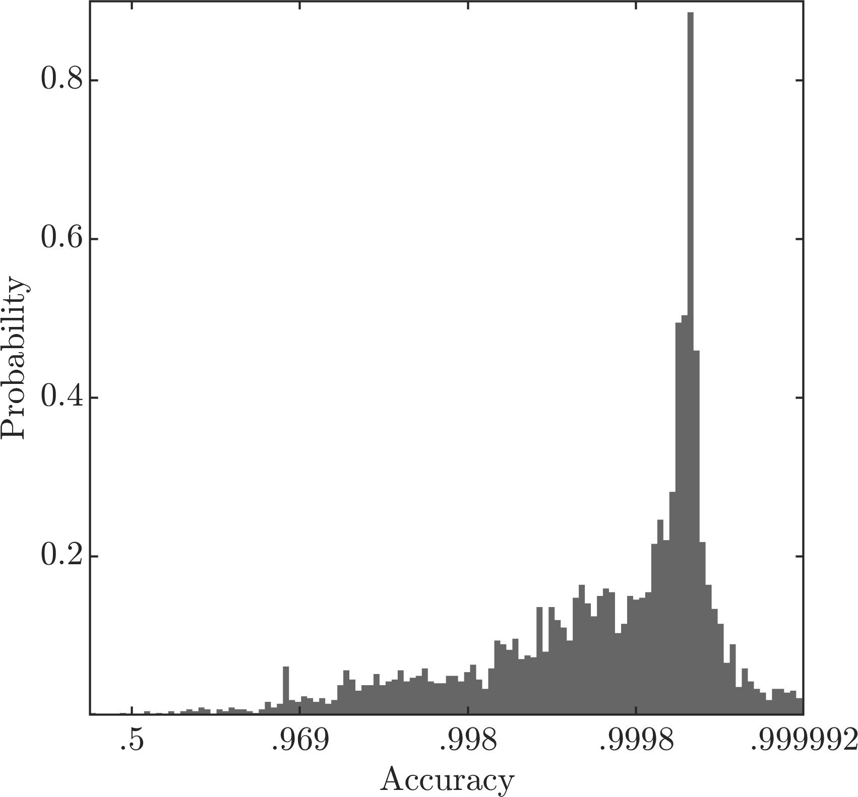
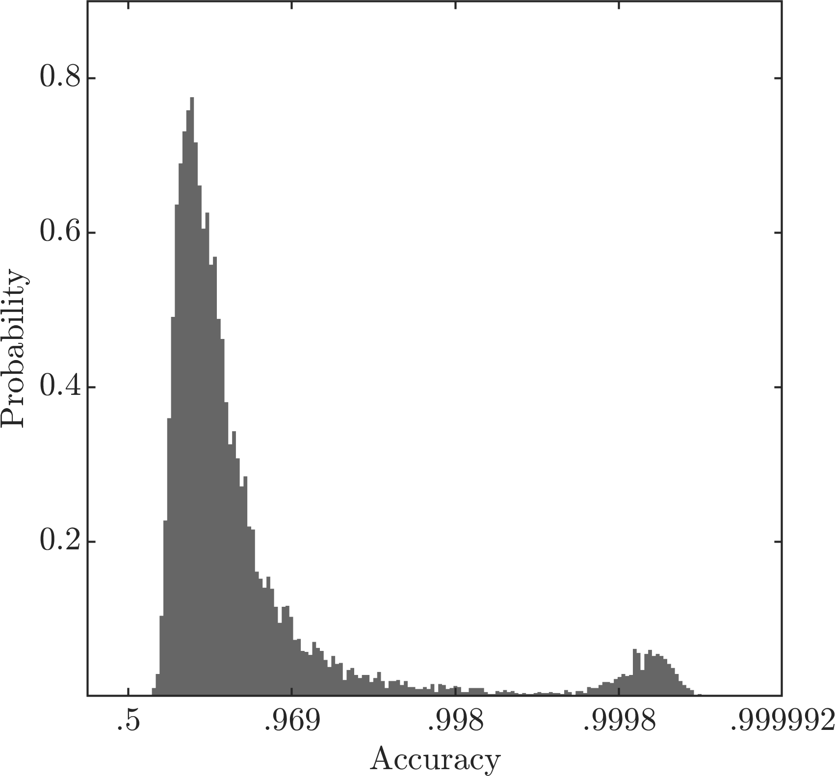
Figure 2: Estimated probability density function of the approximation factor of the complex polytope method for two different data sets. The left pictures data set is Dataset $(A)$, the right pictures data set is Dataset $(B)$.

Although the theoretical approximation factor of this method is $\nicefrac{{1}}{{2}}$, in numerical experiments it turns out that the average approximation factor is mostly larger than $\nicefrac{{1}}{{\sqrt{2}}}$. In small dimensions, $d=2,3$, the approximation factor is even close to $1$ in a lot of cases, see Figure 2 for the (estimated) probability density function of this methods approximation factors.

Note that the numerical accuracy of the QP solver is approximately $10^{-5}$ and thus, the maximal accuracy which can be reached is approximately $0.99999$, which is quite exactly the position of the rightmost peaks in Figure 2

9.2   
Behaviour of the corner cutting method

The corner cutting method is, like the complex polytope method, a QP problem, and thus, the absolute error of the solution returned by our numerical solvers is in the range of $10^{-5}$. For the corner cutting method, this accuracy is on average obtained after 10 to 12 iterations in the generic case, as our experiments show. Apart from the chosen accuracy, the runtime of the algorithm mostly depends on, firstly, the geometry of the problem and, secondly, on the number of vertices of the elliptic polytope. The dimension of the problem only has a minor influence on the runtime.

9.3   
Behaviour of the Projection Method (Method E)

The absolute error of the LP solvers is roughly $10^{-9}$, which is magnitudes higher than for the QP solver. Solely due to this fact, the projection method is the most accurate method of all the described methods.

For the projection method one could increase the number of vertices of the polytopes approximating the ellipses of the elliptic polytope until the norm is computed up to the desired accuracy, similar as in the corner cutting method. Unfortunately, this hinders the use of warm-starting the LP problem since this alters the underlying LP. Therefore, in our implementation we choose the approximation factor $q_{1}$ corresponding to Problem EE* to be of the same magnitude than the approximation factor $q_{2}$ corresponding to Problem EE, and such that $q_{1}q_{2}\simeq q$, where $q$ is the chosen accuracy.

10   

Applications

10.1   
Number of extremal vertices

Before we demonstrate the main applications, the construction of Lyapunov functions of linear systems and evaluation of extremal norms, we address the question of the expected number of vertices in the convex hull of random ellipses. This issue is important for both of the above applications since it shows the growth of the number of ellipses with respect to the number of the iterations of the algorithms.

The corresponding problem for the convex hull of random points originated with the famous question of Sylvester [27]. The answer highly depends on the domain on which the points are sampled and on the dimension. Various lower and upper bounds on the asymptotically expected number of points in the convex hull are known, see [16][4] and references therein. It would be extremely interesting to come up with similar theoretical estimates for convex hulls of ellipses. Here we compare the two cases solely numerically. There is no canonical analogue between points sampled from some domain and ellipses sampled from some domain, since the ellipses are determined by two parameters instead of one. We introduce several numerical results with various samplings.

Uniform sampled ellipsoids in the unit ball

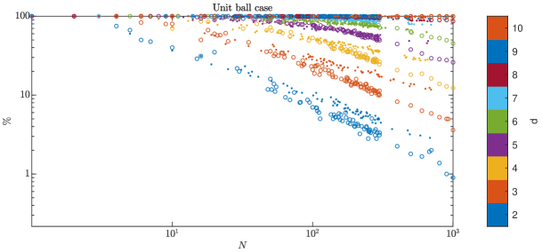
Figure 3: Fraction of points or ellipses which belong to the convex hull of randomly selected points or ellipses which are uniformly distributed in the unit ball or have uniformly distributed real and imaginary part in the unit ball, respectively.

Given ellipses whose real and imaginary part are sampled uniformly from the unit ball, and given points uniformly sampled from the unit ball. The number of vertices and ellipses of their corresponding convex hull is plotted in Figure 3. Experiments are made for dimensions 2 to 10 and number of points and ellipses 1 to 1000. Since the computational time increases significantly with the number of points or ellipses, for sets with more than 300 points or ellipses less examples were conducted. In the plot one can see the relative fraction of points or ellipses belonging to the convex hull, coloured with respect to the dimension. The point examples are plotted with a $\cdot$ symbol, the ellipse examples are plotted with a $\circ$ symbol.

Interestingly, the two cases differ greatly. Whereas for dimensions 2 to 5 the fraction of ellipses belonging to the convex hull is less than for the point counterpart, the situation is reversed from dimension 7 upwards.

Uniform sampled ellipsoids in the unit cube

Interestingly, when the points or the real and imaginary parts of the ellipses are sampled uniformly from a unit-cube, the behaviour between the point case and the ellipses is very similar, at least for small dimensions, as can be seen in Figure 4.

Figure 4: Fraction of points or ellipses which belong to the convex hull of randomly selected points or ellipses which are uniformly distributed in the unit cube or have uniformly distributed real and imaginary part in the unit cube, respectively.

Gaussian sampled ellipsoids

Also for points and ellipses with real and imaginary part sampled from a $d$-dimensional normal distribution, the behaviour is similar. See Figure 5 for a visualization of the obtained numerical results.

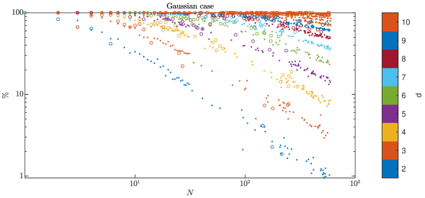
Figure 5: Fraction of points or ellipses which belong to the convex hull of randomly selected points or ellipses which are normal distributed or have normal distributed real and imaginary part, respectively.

10.2   
Lyapunov function for a discrete time linear system

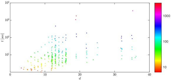
Figure 6: The computation time for evaluating an invariant elliptic polytope $P$ for a given matrix $A$ with complex leading eigenvalue such that $AP\subset\rho(A)P$ holds. The colour indicates the number of vertices of the polytope.

Given a linear system defined by a $d\times d$ matrix $A$ with a complex leading eigenvalue, which is supposed to be unique and simple. We need to construct a norm $\|\cdot\|$ in ${\mathbb{R}}^{d}$ such that $\|A{\boldsymbol{x}}\|\,\leq\,\rho(A)\|{\boldsymbol{x}}\|$ for all ${\boldsymbol{x}}\in{\mathbb{R}}^{d}$. This is the same as constructing a symmetric convex body $P\subset{\mathbb{R}}^{d}$ for which $AP\subset\rho(A)P$. It is obtained as an elliptic polytope by an iteration method, see Section 1, Application 2. In Figure 6 the time needed to compute the invariant elliptic polytope $P$ is plotted against the dimension. The colour indicates the number of vertices of the set $V$.

10.3   
Invariant polytope algorithm

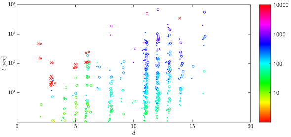
Figure 7: The time of computation of the joint spectral radius for a pair of matrices $A_{1},A_{2}\in{\mathbb{R}}^{d}$, whose spectrum maximizing product has complex leading eigenvalue. The colour indicates the number of vertices of the polytope.

Now we analyse the performance of the Invariant polytope algorithm for computation of the joint spectral radius of a set of matrices. The elliptic polytopes are applied in the case when the spectrum maximizing product has a complex leading eigenvalue. In the construction of the invariant elliptic polytopes we can use each of our methods. The numerical tests show that the projection method always performs better than the corner cutting method and that the mixed method always performs better than the projection method. Thus, only two significant algorithms remain, the complex polytope method and the projection method. We are comparing them.

In Figure 7 the results of our experiments are plotted. On the x-axis we have the dimension of the generated example, the y-axis shows the time needed to compute an invariant polytope. The x-values are slightly distorted for better readability. Similar to the case of random matrices with real leading eigenvalue, it seems that the existence of a spectrum maximizing product with finite length is generic. The results obtained using the complex-polytope method are marked with a $\cdot$ symbol, the results obtained using the projection method are marked with a $\circ$ symbol. Examples where the algorithm could not find an invariant polytope are marked in both cases with a red $\color[rgb]{1,0,0}\times$ symbol. We suspect the reason why the Invariant polytope algorithm may not terminate within reasonable time for certain examples is a long spectrum maximizing product for the set under test.

Remark 10.1.

In practice it occurs rather seldom that a spectrum maximizing product of a set of matrices possesses a complex leading eigenvalue and whose length is greater than one. One such example is given in the Appendix, Example A.3.

Appendix A Appendix

Proof of Theorem 3.4.

We begin with the following technical fact. Let us have a vector ${\boldsymbol{a}}\in{\mathbb{R}}^{2}$ and a line $\ell$ on ${\mathbb{R}}^{2}$ which is not parallel to ${\boldsymbol{a}}$. An affine symmetry about $\ell$ along ${\boldsymbol{a}}$ is an affine transform that for each ${\boldsymbol{x}}\in\ell$ and $t\in{\mathbb{R}}$, maps the point ${\boldsymbol{x}}+t{\boldsymbol{a}}$ to ${\boldsymbol{x}}-t{\boldsymbol{a}}$. If ${\boldsymbol{a}}\perp\ell$, then this is the usual (orthogonal) symmetry.

Lemma A.1.

Let $O$ be an arbitrary point on the side of a convex polygon different from its midpoint. Then there exists an affine symmetry about this side arbitrarily close to an orthogonal symmetry such that the distances from $O$ to the images of the vertices of this polygon are all different.

Proof.

If we choose the origin at $O$ and one of the basis vectors along that side, then the matrix of an arbitrary affine symmetry is

$$S\ =\ \left(\begin{array}[]{rr}1&a\\ 0&-1\end{array}\right)\,,$$

where $a$ is an arbitrary number. If the images $A{\boldsymbol{x}}$ and $A{\boldsymbol{y}}$ of two vertices ${\boldsymbol{x}}\neq{\boldsymbol{y}}$ are equidistant from $O$, then the vectors $A({\boldsymbol{x}}+{\boldsymbol{y}})$ and $A({\boldsymbol{x}}-{\boldsymbol{y}})$ are orthogonal and hence $({\boldsymbol{x}}-{\boldsymbol{y}})A^{T}A({\boldsymbol{x}}+{\boldsymbol{y}})=0$. This is a quadratic equation in $a$, which has at most two solutions. Hence, there exists only a finite number of values of $a$ for which some of images of vertices are equidistant from $O$. ∎

Proposition A.2.

For every $n\geq 2$ and $\varepsilon>0$, there exists a polyhedron $Q_{n}$ in ${\mathbb{R}}^{n+2}$ with at most $2n+3$ facets whose orthogonal projection to some two-dimensional plane is a $2^{n}$-gon such that: 1) Its distance (in the Hausdorff metric) to a regular $2^{n}$-gon centred at the origin is less than $\varepsilon$. 2) The distances from its $2^{n}$ vertices to the origin are all different.

Proof.

Applying the construction (14) for $r=1$, we obtain a polyhedron that consists of points $(x_{1},\ldots,x_{2n+2})^{T}\in{\mathbb{R}}^{2n+2}$ satisfying the system (14). That system contains $n$ linear equations and $2n+3$ linear inequalities. Hence, it defines an $(n+2)$-dimensional polyhedron with at most $2n+3$ facets. Its projection to the plane $(x_{2n+1},x_{2n+2})$ is a regular $2^{n}$-gon. Now, in each iteration $j=1,\dots,n$ of the construction (14), we replace the symmetry about the line $\ell_{\alpha_{n-j+1}}$ by a close affine symmetry about the same line. Invoking Lemma A.1 we can choose this symmetry so that the resulting polygon has all its vertices on different distances from the origin. Hence, the polygon obtained after the last iteration also possesses this property. ∎

Proof of Theorem 3.4..

After applying Proposition A.2 for $n=N-2$, we obtain a polyhedron $Q_{N-2}\subset{\mathbb{R}}^{N}$ whose two-dimensional projection to the plane $(x_{2N-3},x_{2N-2})$ is a $2^{N-2}$-gon close to a regular $2^{N-2}$-gon. Then for the quadratic form $x_{2N-3}^{2}+x_{2N-2}^{2}$, each vertex of this polygon is a local maximum and all the values in those points are different. ∎

Set of matrices with spectral maximizing product of length 2

Example A.3.

For $\alpha,\beta\in(-\pi/2,\pi/2)$, $\alpha\neq\beta$, the set $\{T_{0},T_{1}\}$,

$$T_{0}=\begin{pmatrix}0&0&0\ \\ -\sin\,\alpha&\cos\,\alpha&0\ \\ \phantom{-}\cos\,\alpha&\sin\,\alpha&0\ \end{pmatrix},\quad T_{1}=\begin{pmatrix}\ 0&-\sin\,\beta&\cos\,\beta\ \\ \ 0&\phantom{-}\cos\,\beta&\sin\,\beta\ \\ \ 0&0&0\ \end{pmatrix},$$

has $T_{0}T_{1}$ as spectrum maximizing product, i.e. up to permutations and powers the normalized spectral radius of all other products of matrices $T_{0}$ and $T_{1}$ is strictly less than $\rho(T_{0}T_{1})^{1/2}=1$.

References

- [1] N. E. Barabanov, Lyapunov indicator for discrete inclusions, I-III, Autom. Remote Control, 49 (1988) 2, 152–157.
- [2] A. Ben-Tal, A. Nemirovski, On polyhedral approximations of the second-order cone, Math. Oper. Res., 26 (2001) 2, 193–205, doi: 10.1287/moor.26.2.193.10561.
- [3] M. Charina, C. Conti, T. Sauer, Regularity of multivariate vector subdivision schemes, Num. Algor., 39 (2005), 97–113, doi: 10.1007/s11075-004-3623-z.
- [4] D. L. Donoho, J. Tanner Counting faces of randomly projected polytopes when the projection radically lowers dimension, J. Amer. Math. Soc., 22 (2009), 1–53, doi: 10.1090/S0894-0347-08-00600-0.
- [5] J.-A. Ferrez, K. Fukuda, Th. M. Liebling, Solving the fixed rank convex quadratic maximization in binary variables by a parallel zonotope construction algorithm, European J. Oper. Res., 166 (2005) 1, 35–50, doi: 10.1016/j.ejor.2003.04.011.
- [6] R. Gielen, M. Lazar, On stability analysis methods for large-scale discrete-time systems, Automatica J. IFAC, 55 (2015), 6–72, doi: 10.1016/j.automatica.2015.02.034.
- [7] M. X. Goemans, D. P. Williamson, Improved approximation algorithms for maximum cut and satisfiability problems using semidefinite programming, J. ACM, 42 (1995) 6, 1115–1145, doi: 10.1145/227683.227684.
- [8] E. S. Gorskaya, Approximation of convex functions by projections of polyhedra, Moscow Univ. Math. Bull., 65 (2010) 5, 196–203, doi: 10.3103/S0027132210050049.
- [9] N. Guglielmi , V. Yu. Protasov, Exact computation of joint spectral characteristics of linear operators, Found. Comput. Math., 13 (2013) 1, 37–97, doi: 10.1007/s10208-012-9121-0.
- [10] N. Guglielmi, V. Yu. Protasov, Invariant polytopes of sets of matrices with applications to regularity of wavelets and subdivisions, SIAM J. Matr. Anal. Appl., 37 (2016) 1, 18–52, doi: 10.1137/15M1006945.
- [11] N. Guglielmi, F. Wirth, M. Zennaro, Complex polytope extremality results for families of matrices, SIAM J. Matrix Anal. Appl., 27 (2005), 721–743, doi: 10.1137/040606818.
- [12] N. Guglielmi, M. Zennaro, Balanced complex polytopes and related vector and matrix norms, J. Convex Anal., 14 (2007), 729–766.
- [13] N. Guglielmi, M. Zennaro, Finding extremal complex polytope norms for families of real matrices, SIAM J. Matrix Anal. Appl., 31 (2009) 2, 602–620, doi: 10.1137/080715718.
- [14] N. Guglielmi, M. Zennaro, Canonical construction of polytope Barabanov norms and antinorms for sets of matrices, SIAM J. Matrix Anal. Appl., 36 (2015) 2, 634–655, doi: 10.1137/140962814.
- [15] L. Gurvits, Stability of discrete linear inclusions, Lin. Alg. Appl., 231 (1995), 47–85, doi: 10.1016/0024-3795(95)90006-3.
- [16] I. Hueter, Limit theorems for the convex hull of random points in higher dimensions, Trans. Amer. Math. Soc., 351 (1999) 11, 4337–4363, doi: 10.1090/S0002-9947-99-02499-X.
- [17] J. Håstad, Clique is hard to approximate within , Acta Math., 182 (1999), 105–142, doi: 10.1007/BF02392825.
- [18] J. Håstad, Some optimal inapproximability results, J. ACM., 48 (2001), 798–859., doi: 10.1145/502090.502098.
- [19] R. Jungers, The joint spectral radius. Theory and applications, Lecture Notes in Control and Information Sciences (2009), Springer, ISBN: 978-3-540-95980-9.
- [20] V. S. Kozyakin, Structure of extremal trajectories of discrete linear systems and the finiteness conjecture, Automat. Remote Control, 68 (2007), 174–209, doi: 10.1134/S0005117906040171.
- [21] T. Mejstrik, Improved invariant polytope algorithm and applications, ACM Trans. Math. Softw., 46 (2020) 3 (29), 1–26, doi: doi.org/10.1145/3408891.
- [22] T. Mejstrik, Matlab toolbox for work with subdivision schemes and joint spectral radius, GitLab, gitlab.com/tommsch.
- [23] T. Mejstrik, C. Hollomey, TTEST framework - unit test framework for Matlab/Octave, GitLab, gitlab.com/tommsch/TTEST.
- [24] E. Plischke, F. Wirth, Duality results for the joint spectral radius and transient behaviour, Lin. Alg. Appl., 428 (2008), 2368–2384, doi: 10.1109/CDC.2005.1582512.
- [25] V. Yu. Protasov, The joint spectral radius and invariant sets of linear operators, Fundamentalnaya i prikladnaya Matematika, 2 (1996) 1, 205–231, Link: mi.mathnet.ru/eng/fpm/v2/i1/p205.
- [26] V. Yu. Protasov, The Euler binary partition function and subdivision schemes, Math. Comp., 86 (2017), 1499–1524, doi: 10.1090/mcom/3128.
- [27] J. J. Sylvester, Problem 1491, The Educational Times (London), April (1864), 1–28.
- [28] F. Wirth, The generalized spectral radius and extremal norms, Lin. Alg. Appl., 342 (2002), 17–40, doi: 10.1016/S0024-3795(01)00446-3.