Lubricated axisymmetric gravity currents of power-law fluids.

Abstract

The motion of glaciers over their bedrock or drops of fluid along a solid surface can become unstable when these substrates are lubricated. Previous studies modeled such systems as coupled gravity currents (GCs) consisting of one fluid that lubricates the flow of another fluid, and having two propagating fronts. When both fluid are Newtonian and discharged at constant flux, global similarity solutions were found. However, when the top fluid is strain-rate softening experiments have shown that each fluid front evolved with a different exponent. Here we explore theoretically and numerically such lubricated GCs in a model that describes the axisymmetric spreading of a power-law fluid on top of a Newtonian fluid, where the discharge of both fluids is power law in time. We find that the model admits similarity solutions only in specific cases, including the purely Newtonian case, for a certain discharge exponent, at asymptotic limits of the fluids viscosity ratio, and at the vicinity of the fluid fronts. Generally, each fluid front has a power-law time evolution with a similar exponent as a non-lubricated GC of the corresponding fluid, and intercepts that depend on both fluid properties. Consequently, we identify two mechanisms by which the inner lubricating fluid front outstrips the outer fluid front. Many aspects of our theory are found consistent with recent laboratory experiments. Discrepancies suggest that hydrofracturing or wall slip may be important near the fronts. This theory may help to understand the dynamics of various systems, including surges and ice streams.

1 Introduction

Gravity-driven flows of one fluid over another can involve complex interactions between the two fluids, which can lead to a rich dynamical behavior. Such flows occur in a wide range of natural and human-made systems, as in lava flow over less viscous lava (Griffiths, 2000; Balmforth et al., 2000), spreading of the lithosphere over the mid-mantle boundary (Lister & Kerr, 1989; Dauck et al., 2019), ice flow over an ocean (DeConto & Pollard, 2016; Kivelson et al., 2000) and over bedrock consisting of sediments and water (Stokes et al., 2007; Fowler, 1987), flows in permeable rocks (Woods & Mason, 2000), liquid drops deforming over lubricated surfaces (Daniel et al., 2017), and droplets motion on liquid-infused surfaces (Keiser et al., 2017).

The flow of GCs in circular geometry has been studied with a range of boundary conditions. In the absence of a lubricating layer, a common boundary condition along the base of a sole GC is no slip. Such GCs of Newtonian fluids that are discharged at a rate proportional to $t^{\alpha}$, where $t$ is time and $\alpha$ is a non-negative scalar, has a similarity solution in which the front evolves proportionally to $t^{(3\alpha+1)/8}$ (Huppert, 1982). Similar axisymmetric gravity currents of power-law fluids having exponent $n$, where $n=1$ represents a Newtonian fluid and $n>1$ represents a strain-rate softening fluid, also have similarity solutions in which the front propagation is proportional to $t^{[\alpha(2n+1)+1]/(5n+3)}$ (Sayag & Worster, 2013).

On the other extreme, the presence of a lower fluid layer can significantly reduce friction at the base of the top fluid, resulting in extensionally dominated GCs. This is the case, for example, for ice shelves, which deform over the relatively inviscid oceans with weak friction along their interface. The late-time front evolution of such axisymmetric GCs of Newtonian fluids is proportional to $t$ and is believed to be stable (Pegler & Worster, 2012). However, when the top fluid is strain-rate softening, an initially axisymmetric front can destabilise and develop fingering patterns that consist of tongues separated by rifts (Sayag & Worster, 2019).

In the more general case friction along the base of GCs can vary spatiotemporally, as their stress field evolves. For example, the interface of an ice sheet with its underlying bed rock can include distributed melt water and sediments, which impose nonuniform and time-dependent friction along the ice base, and evolve spatiotemporally under the stresses imposed by the ice layer (Schoof & Hewitt, 2013; Fowler, 1981). Consequently, the coupled ice-lubricant system may evolve various flow patterns such as ice streams (Stokes et al., 2007; Kyrke-Smith et al., 2013) and glacier surges (Fowler, 1987). Such flows were also modelled as two coupled GCs of Newtonian fluids spreading axisymmetrically one on top of the other (Kowal & Worster, 2015). The early stage of these flows follows a self-similar evolution, in which the fronts of the two fluids evolve like $t^{1/2}$, as in non-lubricated (no-slip) GCs (Huppert, 1982), but they can have a radially non-monotonic thickness. Furthermore, laboratory experiments were found to be consistent with the similarity solutions after an initial transient state, but at a later stage they became unstable and developed fingering patterns (Kowal & Worster, 2015). It has been suggested that such instabilities appear when the jump in hydrostatic pressure gradient across the lubrication front is negative (Kowal & Worster, 2019a, b).

Despite the wide range of natural lubricated GCs that involve non-Newtonian fluids, the radial flow of a non-Newtonian fluid over a lubricated layer of Newtonian fluid has just recently been explored experimentally (Kumar et al., 2021). Motivated by glacier flow over lubricated bedrock, the experimental setup consisted of a GC of a strain-rate-softening fluid (Xanthan-gum solution) that has a power-law viscous deformation similar to ice (Glen, 1952), and a lubricating GC of a less viscous Newtonian fluid (diluted sugar solution). The pattern of both fluids in those constant-flux $(\alpha=1)$ experiments remained axisymmetric throughout the flow (Figure 1), in contrast to the fingering pattern that emerged in the purely Newtonian experiments (Kowal & Worster, 2015), as long as the flux ratio of the lubricating fluid to the non-Newtonian fluid was lower than $\sim 0.06$. The fronts of the two fluids appeared to have a power-law time evolution with different exponents. Particularly, the front of the top non-Newtonian fluid evolved with the same exponent $(2n+2)/(5n+3)$ as a non-lubricated power-law fluid (Sayag & Worster, 2013), whereas the front of the Newtonian lubricating fluid evolved with an exponent $1/2$ similar to a Newtonian non-lubricated GC (Huppert, 1982). Despite the similarity of the exponents, the fronts of those lubricated GCs evolved faster than the corresponding non-lubricated GCs owing to larger intercepts. In addition, in contrast with the monotonically declining thickness of non-lubricated GCs, the thickness of the lubricated, non-Newtonian fluid was found to be nearly uniform in the lubricated part of the flow, while that of the lubricating fluid was non-monotonic with localised spikes.

Following up the experimental study of Kumar et al. (2021), here we develop the theory for lubricated axisymmetric GCs of power-law fluids, and explore its major consequences. Specifically, we develop a mathematical model for axisymmetric flow of a viscous gravity current of a power-law fluid lubricated by a Newtonian gravity current, considering a general input flux of the form $t^{\alpha}$, and show that in the general case the flow has no global similarity solution of the 1st kind (§2). We then describe the numerical solver (§3) and investigate several special cases that have similarity solutions (§4). We then explore the possibility that the inner lubricating front outstrip the outer front (§5). Finally, we investigate the case of constant flux discharge (§6), and compare our theoretical predictions with the laboratory experiments of Kumar et al. (2021) (§7).

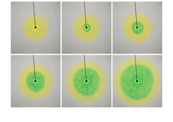
Figure 1: Snapshots from a laboratory experiment (Kumar et al., 2021) of a lubricated GC that consists of a strain-rate softening fluid (yellow) lubricated by a sugar solution (blue, appears green). Marked time at each snapshot is relative to the initiation time $t_{L}$ of the lubricating fluid.

2 Mathematical Model

Consider a power-law fluid having viscosity $\mu$ and density $\rho$ that spreads axisymmetrically under its own weight over a horizontal rigid surface. Simultaneously, a lubricating film of Newtonian fluid of viscosity $\mu_{\ell}$ and density $\rho_{\ell}$ spreads axisymmetrically over the substrate and below the power-law fluid (Figure 2). Both fluids are discharged at the origin of a cylindrical coordinate system in which $r$ is the radial coordinate and $z$ the vertical coordinate. The upper and lower fluid fronts are denoted by $r_{N}(t)$ and $r_{L}(t)$ respectively, and the corresponding fluid thicknesses are denoted by $H(r,t)-h(r,t)$ and $h(r,t)$ respectively, where $t$ is the time variable. Beginning the discharge of the lubricating fluid at a time delay $t_{L}$ with respect to the upper fluid, creates two regions in the flow: an inner, lubricated region ($r\leq r_{L}$) in which the power-law fluid flows at a finite velocity along the interface with the lubricating fluid, and an outer, non-lubricated region ($r_{L}<r\leq r_{N}$) in which the power-law fluid meets the substrate and has zero velocity along it.

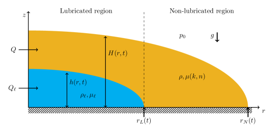
Figure 2: Diagram illustrating a GC of Newtonian fluid (blue) lubricating a GC of a power-law fluid (yellow).

Assuming that the radial extent of the flow is much greater than its thickness in both fluid layers, we can apply the lubrication approximation, which implies that the flow is primarily horizontal (a GC) and that the dominant strain rate in each fluid layer $i$ is $\partial u_{i}/\partial z$, where $u_{i}(r,z,t)$ is the radial velocity component. Therefore, the axisymmetric Cauchy equations for each fluid layer, simplified for flows of low Reynolds numbers and lubrication approximations are

$$\frac{\p p_{i}}{\p r} = \frac{\p}{\p z}\left(\mu_{i}\frac{\p u_{i}}{\p z}\right),$$ (1a)

$$\frac{\p p_{i}}{\p z} = -\rho_{i}g,$$ (1b)

$$\frac{1}{r}\frac{\p(ru_{i})}{\p r}+\frac{\p w_{i}}{\p z} = 0,$$ (1c)

to leading order, where $w_{i}$ is the vertical velocity component, $p_{i}$ is the pressure field, and $g$ is the gravitational acceleration. The pressure is determined hydrostatically in equation 1b because we assume a large Bond number, implying that the effects of surface tension are negligible compared to gravity. We note that equations 1 satisfy the lubrication approximation, so this model does not accurately describe the problem at early times, before the fluid radial extent is sufficiently greater than its thickness.

The viscosity of the power-law fluid is determined by

$$\mu=k\left(\frac{1}{2}\textbf{e}:\textbf{e}\right)^{\textstyle{\frac{1}{2}\left({\frac{1}{n}-1}\right)}},$$ (2)

where e is the strain-rate tensor, $k$ is the consistency coefficient, and $n$ is the power-law exponent, which determines the fluid’s response to stress. Specifically, $n=1$ represents a Newtonian fluid with dynamical viscosity $k$, $n>1$ a shear-thinning fluid, and $n<1$ a shear-thickening fluid. In the lubrication limit $\textbf{e}:\textbf{e}\approx\left(\partial u/\partial z\right)^{2}$ to leading order, so that the viscosity of the power-law fluid simplifies to

$$\mu=k\left|\frac{1}{2}\frac{\partial u}{\partial z}\right|^{\textstyle{\frac{1}{n}-1}}.$$ (3)

We assume that the total volumes of the power-law fluid and the Newtonian fluid evolve following a power law in time given by

$$2\pi\int_{0}^{r_{N}}(H-h)r~{}dr=Qt^{\alpha},$$ (4a)

$$2\pi\int_{0}^{r_{L}}hr~{}dr=Q_{\ell}\left(t-t_{L}\right)^{\alpha},$$ (4b)

respectively, where $\alpha$ is a constant exponent, and $Q$ and $Q_{\ell}$ are constant coefficients representing, for instance, the discharge flux of each fluid when $\alpha=1$.

2.1 The Non-Lubricated Region

In the non-lubricated region, the power-law fluid meets the substrate and the lubricating fluid is absent. Integrating 1b, the pressure distribution is

$$p(z,r,t)=p_{0}+\rho g(H(r,t)-z),$$ (5)

where $p_{0}$ is the ambient pressure over the top free surface of the power-law fluid. Integration of the radial force balance (1a) across the depth of the fluid layer together with no-slip boundary conditions along the substrate and no stress along the free surface

$$u(z=0)=0,\quad\mu\frac{\partial u}{\partial z}(z=H)=0,$$ (6)

gives the radial velocity field

$$u(z,r,t)=2^{{{1-n}}}\left(\frac{\rho g}{k}\right)^{{n}}\frac{\partial H}{\partial r}\left|\frac{\partial H}{\partial r}\right|^{{n-1}}\frac{1}{1+n}\left[(H-z)^{{n+1}}-H^{{n+1}}\right].$$ (7)

Similar integration of the continuity equation (1c), accounting for a free surface at the upper boundary $z=H(r,t)$, and assuming no normal flow through the substrate, gives the Reynolds equation

$$\frac{\p H}{\p t}+\frac{1}{r}\frac{\p(rq)}{\p r}=0,$$ (8)

which should satisfy the boundary conditions

$$H(r=r_{N})=0\quad\textrm{and}\quad q(r=r_{N})=0,$$ (9)

where the local flux $q$ is determined using eq. 7 to give

$$q=\int^{H}_{0}u~{}dz=-2^{1-n}\left(\frac{\rho g}{k}\right)^{{n}}\frac{\p H}{\p r}\left|\frac{\p H}{\p r}\right|^{{n-1}}\frac{1}{n+2}H^{{n+2}}.$$ (10)

2.2 The Lubricated Region

As in the non-lubricated region and assuming continuity of pressure at the fluid-fluid interface $z=h$, the pressure in the lubricated region is determined hydrostatically by

$$p(z)=p_{0}+\rho g(H-z), \quad\textrm{where}\quad h\leq z\leq H,$$ (11a)

$$p_{\ell}(z)=p_{0}+\rho g(H-h) +\,\rho_{\ell}g(h-z), \quad\textrm{where}\quad 0\leq z\leq h.$$ (11b)

The radial force balances simplify to

$$\frac{k}{2^{{\frac{1}{n}-1}}}\frac{\partial}{\partial z}\left(\frac{\partial u}{\partial z}\left|\frac{\partial u}{\partial z}\right|^{\textstyle{\frac{1}{n}-1}}\right) = \frac{\partial p}{\partial r},\quad\textrm{where}\quad h\leq z\leq H,$$ (12a)

$$\mu_{\ell}\frac{\partial^{2}u_{\ell}}{\partial z^{2}} = \frac{\partial p_{\ell}}{\partial r},\quad\textrm{where}\quad 0\leq z\leq h,$$ (12b)

together with the boundary conditions,

$$u_{\ell}=0, \quad\textrm{where}\quad z=0,$$ (13a)

$$u_{\ell}=u,\qquad k\left|\frac{1}{2}\frac{\p u}{\p z}\right|^{\textstyle{\frac{1}{n}-1}}\frac{\p u}{\p z}=\mu_{\ell}\frac{\partial u_{\ell}}{\partial z}, \quad\textrm{where}\quad z=h,$$ (13b)

$$\frac{\partial u}{\partial z}=0, \quad\textrm{where}\quad z=H,$$ (13c)

which represent, respectively, no-slip along the solid substrate, continuous flow velocity and shear stress at the fluid-fluid interface, and no shear stress along the free surface of the power-law fluid. Integrating the radial force balance (equations 12) across the thickness of each fluid layer, and using the boundary conditions (equations 13) we get the radial velocity fields in each fluid layer

$$u(z,r,t) = 2^{1-n}\left(\frac{\rho g}{k}\right)^{{n}}\frac{1}{1+n}\frac{\partial H}{\partial r}\left|\frac{\partial H}{\partial r}\right|^{n-1}\left[(H-z)^{{1+n}}-(H-h)^{{1+n}}\right]$$

$$-\frac{\rho g}{\mu_{\ell}}\left[\frac{\partial H}{\partial r}\left(Hh-\frac{h^{2}}{2}\right)+\frac{h^{2}}{2}\frac{\rho_{\ell}-\rho}{\rho}\frac{\partial h}{\partial r}\right],$$

$$u_{\ell}(z,r,t) = -\frac{\rho g}{\mu_{\ell}}\left[\frac{\partial H}{\partial r}\left(Hz-\frac{z^{2}}{2}\right)+\frac{1}{2}\frac{\rho_{\ell}-\rho}{\rho}\frac{\partial h}{\partial r}\left(2hz-z^{2}\right)\right].$$ (14b)

The Reynolds equations corresponding to each fluid layer have a similar form as that of the non-lubricated region

$$\frac{\partial h}{\partial t}+\frac{1}{r}\frac{\partial(rq_{\ell})}{\partial r} = 0,$$ (15a)

$$\frac{\partial(H-h)}{\partial t}+\frac{1}{r}\frac{\partial(rq)}{\partial r} = 0,$$ (15b)

and should satisfy the boundary conditions

$$h=0,\quad q_{\ell}=0\quad \textrm{at}\quad r=r_{L},$$ (16a)

$$\textrm{and }\quad q^{+}=q^{-},\quad H^{+}=H^{-}\quad \textrm{at}\quad r=r_{L},$$ (16b)

where equation 16b signifies flux and height continuity across $r_{L}$. The local fluxes result from integrating equations 14 to get

$$q=\int_{h}^{H}u~{}dz = -2^{1-n}\left(\frac{\rho g}{k}\right)^{{n}}\frac{\partial H}{\partial r}\left|\frac{\partial H}{\partial r}\right|^{{n-1}}\frac{1}{n+2}(H-h)^{{n+2}}$$ (17a)

$$-(H-h)\frac{h\rho g}{\mu_{\ell}}\left[\frac{\partial H}{\partial r}(H-h)+\frac{h}{2}\left(\frac{\partial H}{\partial r}+\frac{\rho_{\ell}-\rho}{\rho}\frac{\partial h}{\partial r}\right)\right],$$

$$q_{\ell}=\int_{0}^{h}u_{\ell}~{}dz = -\frac{h^{2}}{2}\frac{\rho g}{\mu_{\ell}}\left[\frac{\partial H}{\partial r}(H-h)+\frac{2h}{3}\left(\frac{\partial H}{\partial r}+\frac{\rho_{\ell}-\rho}{\rho}\frac{\partial h}{\partial r}\right)\right].$$ (17b)

We note that without a lubricant, this set of PDEs is reduced to the non-lubricated region, and that this PDE set is consistent with the non-lubricated power-law GC model (Sayag & Worster, 2013), which converges to the Newtonian non-lubricated GC when $n=1$ and the fluid dynamic viscosity is $k=\mu$ (Huppert, 1982). In addition, the full PDE set, for the Newtonian case ($n=1$) and constant source fluxes ($\alpha=1$) is consistent with the model for lubricated, Newtonian GCs (Kowal & Worster, 2015).

2.3 Dimensionless Equations

We non-dimensionalize equations 4, 8-10 and 15-17 with the following time, length and height scales

$$t \equiv T\hat{t},$$ (18a)

$$r \equiv \left(\left(\frac{\rho g}{k}\right)^{n}Q^{2n+1}T^{\alpha(1+2n)+1}\right)^{\textstyle{\frac{1}{5n+3}}}\hat{r},$$ (18b)

$$(H,h) \equiv \left(\left(\frac{\rho g}{k}\right)^{-2n}Q^{1+n}T^{\alpha(1+n)-2}\right)^{\textstyle{\frac{1}{5n+3}}}(\hat{H},\hat{h}),$$ (18c)

where hats denote dimensionless quantities. The resulted dimensionless model, dropping hats, in the non-lubricated region $r_{L}\leq r\leq r_{N}$ is

$$\frac{\partial H}{\partial t}+\frac{1}{r}\frac{\partial(rq)}{\partial r}=0,$$ (19)

where

$$q=-\mathscr{N}\frac{\partial H}{\partial r}\left|\frac{\partial H}{\partial r}\right|^{{n-1}}H^{n+2},\qquad\mathscr{N}=\frac{2^{{1-n}}}{n+2},$$ (20)

and in the lubricated region $0\leq r\leq r_{L}$ it is

$$\frac{\partial h}{\partial t}+\frac{1}{r}\frac{\partial(rq_{\ell})}{\partial r} = 0,$$ (21a)

$$\frac{\partial(H-h)}{\partial t}+\frac{1}{r}\frac{\partial(rq)}{\partial r} = 0,$$ (21b)

where

$$q = -\mathscr{N}\frac{\partial H}{\partial r}\left|\frac{\partial H}{\partial r}\right|^{n-1}(H-h)^{2+n}$$ (22a)

$$-\mathscr{M}h(H-h)\left[\frac{\partial H}{\partial r}(H-h)+\left(\frac{\partial H}{\partial r}+\mathscr{D}\frac{\partial h}{\partial r}\right)\frac{h}{2}\right],$$

$$q_{\ell} = -\mathscr{M}\frac{h^{2}}{2}\left[\frac{\partial H}{\partial r}(H-h)+\frac{2h}{3}\left(\frac{\partial H}{\partial r}+\mathscr{D}\frac{\partial h}{\partial r}\right)\right],$$ (22b)

and where the boundary conditions are

$$q=0,\quad H=0\quad \quad r=r_{N},$$ at (23a)

$$q_{\ell}=0,\quad h=0,\quad q^{+}=q^{-},\quad H^{+}=H^{-}\quad \quad r=r_{L},$$ at (23b)

$$\lim_{r\rightarrow 0}(2\pi rq_{\ell})=\alpha\mathscr{Q}\left(t-\hat{t}_{L}\right)^{\alpha-1}\quad\textrm{and}\quad\lim_{r\rightarrow 0}(2\pi rq)=\alpha t^{\alpha-1},$$ (23c)

where $\hat{t}_{L}=t_{L}/T$. The resulted dimensionless quantities

$$\mathscr{Q}\equiv\frac{Q_{\ell}}{Q},\quad\mathscr{D}\equiv\frac{\rho_{\ell}-\rho}{\rho},\quad n,\quad\mathscr{M}\equiv\frac{\mu}{\mu_{\ell}}=\frac{\rho g}{\mu_{\ell}}\left(\frac{k}{\rho g}\right)^{\textstyle{\frac{8n}{5n+3}}}\left(\frac{T^{5-\alpha}}{Q}\right)^{\textstyle{\frac{n-1}{5n+3}}},$$ (24)

represent respectively the discharge flux ratio, the relative density difference of the lubricating and power-law fluids, the power-law fluid exponent, and the dynamic viscosity ratio.

The viscosity ratio 24(iv) implies that the timescale $T$ in (18) is scaled out of the equations in two special cases $n=1$ and $\alpha=5$. This implies that asymptotically in time ($t/t_{L}\gg 1$) our PDE set admits a global similarity solution of the first kind in these two special cases, whereas for any other value of $n$ or $\alpha$, including the constant flux case $(\alpha=1)$, such global similarity solutions do not exist. Nevertheless, as we show in the section that follows (§4), we find several additional asymptotic limits in which part of the flow evolves in a self-similar manner.

In the general case $n\neq 1$ and $\alpha\neq 5$ there are enough relations to determine the time scale $T$ (18) independently of the height and radial scales. This is primarily because the flux in the top fluid layer (22a) consists of two contributions that are not necessarily of the same scale. Requiring that the scales of those two contributions balance $\mathscr{M}(T)=\mathscr{N}$ leads to an independent constraint for the time scale $T$, which upon substitution in (18) leads to a set of independent scales

$$T^{(1-n)(\alpha-5)} = Q^{n-1}\left(\mathscr{N}\frac{\mu_{\ell}}{\rho g}\right)^{5n+3}\left(\frac{\rho g}{k}\right)^{8n},$$ (25a)

$$R^{(1-n)(\alpha-5)} = Q^{2(n-1)}\left(\mathscr{N}\frac{\mu_{\ell}}{\rho g}\right)^{\alpha+1+2\alpha n}\left(\frac{\rho g}{k}\right)^{n(3\alpha+1)},$$ (25b)

$$H^{(1-n)(\alpha-5)} = Q^{n-1}\left(\mathscr{N}\frac{\mu_{\ell}}{\rho g}\right)^{\alpha-2+\alpha n}\left(\frac{\rho g}{k}\right)^{2n(\alpha-1)}.$$ (25c)

Therefore, in the more general case $(n\neq 1$ and $\alpha\neq 5$) there is no global similarity solution of the 1st kind, and the above scales may represent the time, radius and thickness.

3 Numerical Solution

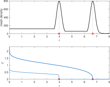
Figure 3: (a) Mesh density and (b) a solution at time $t/t_{L}=100$, showing the lubricated fluid (thick) and the lubricating fluid (thin) for $n=1$, $\mathscr{M}=1$, $\mathscr{Q}=0.2$, and $\mathscr{D}=0.1$. Markers (red) indicate the front positions.

We solve the dimensionless model (eqs. 19 – 24) numerically explicitly using the Matlab PDEPE solver, with an open-ended, non-uniform, and time-dependent adaptive spatial mesh. We find that lower spatial resolution can be used in most of the domain if the mesh is logarithmically spaced, and is denser around the fluid fronts, where the fluid heights drop sharply and the slopes $\p{H}/\p{r}$ and $\p{h}/\p{r}$ become singular. Therefore, we use a non-uniform spatial mesh that consists of two Gaussian distributions centered at the fronts $r_{N}$ and $r_{L}$, and uniform distributions between the origin and $r_{L}$, the two fronts, and beyond $r_{N}$ (Figure 3). The instantaneous front positions $r_{N}(t)$ and $r_{L}(t)$ are determined where $H(r,t)\leq 10^{-6}$ and $h(r,t)\leq 10^{-6}$ respectively. Since the fronts evolve, we enlarge the flow domain progressively and re-mesh the computational grid points every several time steps in order to keep the higher mesh density centered at the front positions. For the re-mesh we predict the front positions in the next time step using a discretization of the front evolution equations

$$\dot{r}_{N}(t)=\lim_{r\rightarrow r_{N}}\frac{q}{H}\quad\textrm{and}\quad\dot{r}_{L}(t)=\lim_{r\rightarrow r_{L}}\frac{q_{\ell}}{h}.$$ (26)

The size of the time step needed in order to solve the PDE is determined by the solver, and we scale $T$ with $t_{L}$, so that $\hat{t}_{L}=1$.

We validated our numerical solver using several known asymptotic solutions. In the limit $\mathscr{Q}=0$ (no lubricating fluid) our model converges to a GC that propagates under no-slip condition along the substrate, which has a similarity solution $r_{N}(t)\propto t^{[\alpha(2n+1)+1]/{(5n+3)}}$ (Huppert, 1982; Sayag & Worster, 2013). We find that our numerical solutions for the fluid heights and for the leading front are consistent with those theoretical predictions (Appendix A). Particularly, discrepancy between the predicted and computed exponents is less than $5\cdot 10^{-3}$ and can be minimized further with a higher spatial resolution. In the limit $n=1$ and $\alpha=1$ our model converges to a purely Newtonian lubricated GC released at constant flux, which has a similarity solution $r_{L},r_{N}\propto t^{1/2}$ (Kowal & Worster, 2015). We find that our numerical solutions are consistent with both the front and thickness predictions for a wide range of $\mathscr{M}$ and $\mathscr{Q}$ values (Appendix A).

4 Similarity solutions

The model described by eqs. 19-24 admits similarity solutions in several special cases. Specifically, global similarity solutions exist when the top fluid is also Newtonian ($n=1$), or when the mass-discharge exponent is $\alpha=5$. In addition, part of the flow evolves in a self-similar manner in the asymptotic limits of the viscosity ratio $\mathscr{M}$. Finally, for any parameter combination the solutions at the vicinity of each front evolve in a self-similar manner.

4.1 The similarity solution for Newtonian fluids $n=1$

When the top fluid is Newtonian ($n=1$) the viscosity ratio $\mathscr{M}$ is independent of $T$, and the resulted purely Newtonian coupled flow admits a global similarity solution. This case, restricted to a constant flux ($\alpha=1$), has been thoroughly explored (Kowal & Worster, 2015). For the general case of $\alpha\geq 0$, the PDE set can be reduced to an ODE set with a similarity variable

$$\eta=\frac{r}{t^{\frac{3\alpha+1}{8}}}\left(\frac{\rho g}{k}Q^{3}\right)^{-\frac{1}{8}},$$ (27)

and a solution of the form

$$\left(H,h\right)=t^{\frac{\alpha-1}{4}}\left(Q\frac{k}{\rho g}\right)^{\frac{1}{4}}\left(F,f\right),$$ (28a)

where $$F f \eta$$ and are dimensionless functions of . Therefore, the fronts of both the lubricated and lubricating fluids evolve like

$$\left(r_{N},r_{L}\right)=\left(\eta_{N},\eta_{L}\right)t^{\frac{3\alpha+1}{8}}\left(Q^{3}\frac{\rho g}{k}\right)^{\frac{1}{8}},$$ (28b)

where $\eta_{N}$ and $\eta_{L}$ are numerical coefficients of order $1$. These solutions have identical structure as the classical solution of Newtonian GCs (Huppert, 1982). Upon substitution, the Reynolds equations (8 and 15) become, for the non-lubricated region ($\eta_{L}\leq\eta\leq\eta_{N}$)

$$\left(\frac{\alpha-1}{4}\right)F-\left(\frac{3\alpha+1}{8}\right)\eta F^{\prime}=\frac{1}{3\eta}\left(\eta F^{\prime}F^{3}\right)^{\prime},$$ (29)

where prime denotes a derivative with respect to $\eta$, and for the lubricated region ($0\leq\eta\leq\eta_{L}$)

$$\left(\frac{\alpha-1}{4}\right)\left(F-f\right)-\left(\frac{3\alpha+1}{8}\right)\eta\left(F^{\prime}-f^{\prime}\right)+\frac{1}{\eta}\left(\eta q\right)^{\prime} = 0,$$ (30a)

$$\left(\frac{\alpha-1}{4}\right)f-\left(\frac{3\alpha+1}{8}\right)\eta f^{\prime}+\frac{1}{\eta}\left(\eta q_{\ell}\right)^{\prime} = 0,$$ (30b)

where

$$q = -\frac{1}{3}F^{\prime}(F-f)^{3}-\mathscr{M}f(F-f)\left[F^{\prime}(F-f)+\frac{1}{2}f\left(\mathscr{D}f^{\prime}+F^{\prime}\right)\right],$$ (31a)

$$q_{\ell} = -\mathscr{M}{f^{2}}\left[\frac{1}{2}F^{\prime}(F-f)+\frac{1}{3}f\left(\mathscr{D}f^{\prime}+F^{\prime}\right)\right].$$ (31b)

The corresponding boundary conditions (23) become

$$F=0,\quad q=0\quad \quad\eta=\eta_{N}$$ at (32a)

$$f=0,\quad q_{\ell}=0,\quad F^{+}=F^{-},\quad q^{+}=q^{-}\quad \quad\eta=\eta_{L},$$ at (32b)

$$\lim_{\eta\rightarrow 0}2\pi\eta q=\alpha,\quad\lim_{\eta\rightarrow 0}2\pi\eta q_{\ell}=\alpha\mathscr{Q},$$ (32c)

where the last condition implies convergence to a similarity solution long time after the initiation of the fluid discharge, $t\gg t_{L}$.

For $\alpha=1$ the model converges to that of Kowal & Worster (2015), and the similarity solutions we predict for general $\alpha$ are consistent with our full numerical solution (Figures 4, 5).

4.2 The similarity solution for mass-discharge exponent $\alpha=5$

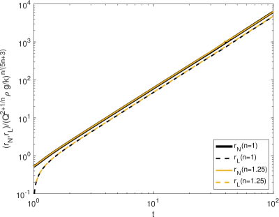
Figure 4: The front propagation verses time for $\alpha=5$, $n=1.25$ and $1$, $\mathscr{Q}=0.2$, $\mathscr{D}=0.1$ and $\mathscr{M}=100$ with curve regression line values indicated on figure, showing that a global similarity solution exists for $\alpha=5$, which is consistent with theoretical prediction of the form $(\eta_{N},\eta_{L})t^{2}$ (eq. 34b).

When the top fluid is non-Newtonian $n\neq 1$ the viscosity ratio $\mathscr{M}$ becomes independent of the time scale $T$ for a discharge exponent $\alpha=5$, and the resulted flow also admits a similarity solution with a similarity variable

$$\eta=\frac{r}{t^{2}}\left[Q^{2n+1}\left(\frac{\rho g}{k}\right)^{n}\right]^{{-1}/{(5n+3)}}$$ (33)

and a solution of the form

$$(H,h)=t\left[Q^{1+n}\left(\frac{k}{\rho g}\right)^{2n}\right]^{{1}/{(5n+3)}}(F,f),$$ (34a)

where $$F f \eta$$ and are dimensionless functions of . Therefore, the fronts of both the lubricated and lubricating fluids evolve like

$$\left(r_{N},r_{L}\right)=\left(\eta_{N},\eta_{L}\right)t^{2}\left[Q^{2n+1}\left(\frac{\rho g}{k}\right)^{n}\right]^{{1}/{(5n+3)}},$$ (34b)

where $\eta_{N}$ and $\eta_{L}$ are numerical coefficients of order $1$. Upon substitution, the Reynolds equations (8 and 15) become, for the non-lubricated region ($\eta_{L}\leq\eta\leq\eta_{N}$)

$$F-2F^{\prime}\eta=\mathscr{N}\frac{1}{\eta}\left(\eta F^{\prime}\left|F^{\prime}\right|^{{n-1}}F^{{n+2}}\right)^{\prime},$$ (35)

and for the lubricated region ($0\leq\eta\leq\eta_{L}$)

$$\left(F-f\right)-2\left(F^{\prime}-f^{\prime}\right)\eta+\frac{1}{\eta}\left(\eta q\right)^{\prime}=0,$$ (36a)

$$f-2f^{\prime}\eta+\frac{1}{\eta}\left(\eta q_{\ell}\right)^{\prime}=0,$$ (36b)

where

$$q = -\mathscr{N}F^{\prime}\left|F^{\prime}\right|^{n-1}\left(F-f\right)^{n+2}-\mathscr{M}f(F-f)\left[F^{\prime}(F-f)+\frac{1}{2}f(\mathscr{D}f^{\prime}+F^{\prime})\right],\qquad$$ (37a)

$$q_{\ell} = -\mathscr{M}{f^{2}}\left[\frac{1}{2}F^{\prime}(F-f)+\frac{1}{3}f(F^{\prime}+\mathscr{D}f^{\prime})\right].$$ (37b)

The corresponding boundary conditions (23) become

$$F=0,\quad q=0\quad \quad\eta=\eta_{N}$$ at (38a)

$$f=0,\quad q_{\ell}=0,\quad F^{+}=F^{-},\quad q^{+}=q^{-}\quad \quad\eta=\eta_{L},$$ at (38b)

$$\lim_{\eta\rightarrow 0}2\pi\eta q=5,\quad\lim_{\eta\rightarrow 0}2\pi\eta q_{\ell}=5\mathscr{Q}.$$ (38c)

Figure 4 shows numerical solution of the full PDE set for $\alpha=5$ for varying power-law exponent values. We find that the numerical solutions are consistent with the predicted similarity solution 34. This consistency further validates the numerical simulation for the combination of lubricated gravity currents with lubricated power-law fluid.

4.3 Similarity solutions for the asymplotic limits in $\mathscr{M}$:
The upper-fluid solid and liquid limits

In the general case of $\alpha\neq 5$ and $n\neq 1$ our model does not admit global similarity solutions of the first kind. However, a similarity solution arises in part of the flow domain in each of the asymptotic limits of the viscosity ratio, in which the upper fluid layer is either relatively more viscous ($\mathscr{M}\gg 1$, the “solid” limit) or relatively less viscous ($\mathscr{M}\ll 1$, the “liquid” limit) compared with the lower fluid layer.

4.3.1 The top-layer solid limit, $\mathscr{M}\gg 1$

The limit $\mathscr{M}\gg 1$ represents the case where the top fluid is much more viscous than the lubricating fluid. One motivation to study this limit is the geophysical setting of ice sheets creeping over less-viscous lubricated beds. In this case, the leading-order scalling of the power-law fluid local flux in the lubricated region (22a) is

$$q\approx-\mathscr{M}h(H-h)\left[\frac{\p H}{\p r}(H-h)+\left(\frac{\p H}{\p r}+\mathscr{D}\frac{\p h}{\p r}\right)\frac{h}{2}\right],$$ (39)

which is identical to the scaling of the Newtonian lubricating fluid flux (22b). In such a case, the three scales $H$, $R$ and $T$ in the lubricated region cannot be determined independently despite the fact that the upper fluid is a power-law fluid. Therefore, both fluids in the lubricated region have a similarity solution in which the dimensionless front in the lubricated region evolves with an $n$-independent exponent

$$r_{L}=\xi_{L}t^{\frac{3\alpha+1}{8}},$$ (40)

where the intercept $\xi_{L}$ may depend on the system dimensionless numbers. The exponent in (40) is consistent with the predictions made for the special cases discussed above. Specifically, for $n=1$ it is $(3\alpha+1)/8$ as we predict in equation (28b), and for $\alpha=5$ it is $2$ independently of $n$ as we predict in equation (34b). This similarity solution does not reveal the evolution of the fluid front $r_{N}$ in the non-lubricated region, which depends on the fluid exponent $n$.

4.3.2 The top-layer “liquid” limit, $\mathscr{M}\ll 1$

The second asymptotic limit, $\mathscr{M}\ll 1$, in which the top fluid is much less viscous than the lubricating fluid, also admits a similarity solution, but of a different sub set of the model. In this case, the leading-order scaling of the power-law fluid local flux in the lubricated region (22a) is

$$q\approx-\mathscr{N}\frac{\partial H}{\partial r}\left|\frac{\partial H}{\partial r}\right|^{{n-1}}(H-h)^{{2+n}},$$ (41)

which is identical to the scaling of the power-law fluid in the non-lubricated region (20). Therefore, the evolution of the power-law fluid in the entire domain converges when $h\ll H$ to the similarity solution of a non-lubricated power-law GC, in which case the upper fluid front evolves with an $n$-dependent exponent

$$r_{N}=\xi_{N}\mathscr{N}^{1/(5n+3)}t^{\textstyle{\frac{\alpha(2n+1)+1}{5n+3}}}$$ (42)

(Sayag & Worster, 2013), where the intercept $\xi_{N}$ may depend on the system dimensionless numbers. This similarity solution does not hold for the lubricating fluid layer since the local flux of the Newtonian lubricating fluid sets a different scaling. Therefore, it does not predict the evolution of the lubricating-fluid front $r_{L}$. For $H-h>1$ the coupling between the upper fluid layer and the lower one grows stronger the more shear-thinning the fluid is ($n\rightarrow\infty$), as the exponent in (41) grows like $n$. Therefore, (42) is expected to be less accurate the more shear-thinning the upper fluid is when $H-h>1$, and more accurate when $H-h<1$.

4.4 Similarity solutions at the vicinity of the fluid fronts

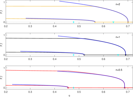
Figure 5: The similarity solutions at the vicinity of the fronts $F(\eta),f(\eta)$ (eqs. 44, 47) based on the non-lubricated theory ($\bullet\bullet\bullet$, blue), compared with the full numerical solution (—) for $\mathscr{M}=100,\mathscr{Q}=0.1,\mathscr{D}=1,\alpha=1$ and $n=0.5,1,2$. The similarity solutions were plotted with respect to the lubricated-theory fronts (${\square},\circ,{\triangle}$ markers at corresponding colors to the $F,f$ curves). For comparison the fronts predicted by the non-lubricated theory are marked ($\bigtriangledown$ (cyan) marks $\eta_{N}$ and $\Diamond$ (cyan) marks $\eta_{L}$).

The thicknesses of the two fluid layers at the vicinity of the fronts have also got self-similar forms, even at the absence of a global similarity solution. These self-similar forms arise because the dynamics at the vicinity of both fronts is dominated by the same dynamics that governs non-lubricated GCs, which are known to have self-similar solutions for any $\alpha$ and $n$ (Sayag & Worster, 2013; Huppert, 1982).

The dominance of a non-lubricated-GC dynamics is naturally expected at the vicinity of the front $r_{N}$, which is the edge of the non-lubricated region in the flow. In this case we expect consistency of the fluid thickness with Sayag & Worster (2013), which implies a similarity solution of the form

$$r = \eta t^{\textstyle{\frac{\alpha(2n+1)+1}{5n+3}}},$$ (43a)

$$H = t^{\textstyle{\frac{\alpha(n+1)-2}{5n+3}}}F\left(\frac{\eta}{\eta_{N}}\right)$$ (43b)

for the model described by equations (19, 20), where $\eta$ is the similarity variable and $\eta_{N}\equiv\eta(r=r_{N})$. Therefore, the asymptotic solution for the function $F$ near the front $\eta_{N}$ in the similarity space is (Sayag & Worster, 2013)

$$F=\left[N\eta_{N}^{n+1}\left(1-\frac{\eta}{\eta_{N}}\right)^{n}\right]^{{1}/{(2n+1)}},\qquad N=\left(\frac{1}{\mathscr{N}}\frac{\alpha(2n+1)+1}{5n+3}\right)^{1/n}\frac{2n+1}{n}.$$ (44)

Near the front $r_{L}$ the dominance of non-lubricated-GC dynamics is also valid, but requires more careful supporting argument. Specifically, we assert that the free surface slope $\p H/\p r$ is finite at $r_{L}$, whereas the slope of the lubricating fluid is singular. Therefore, provided the density difference is non zero, the leading-order flux $q_{\ell}$ (22b) is

$$q_{\ell}=-\frac{\mathscr{M}\mathscr{D}}{3}h^{3}\frac{\p h}{\p r}.$$ (45)

Consequently, the model (21a) for the lubricating fluid near $r_{L}$ is decoupled from $H$, and describes a modified non-lubricated GC of a Newtonian fluid (Huppert, 1982). In this case the thickness $h$ has a similarity solution of the form

$$r = \eta(t-t_{L})^{\textstyle{\frac{3\alpha+1}{8}}},$$ (46a)

$$h = (t-t_{L})^{\textstyle{\frac{\alpha-1}{4}}}f\left(\frac{\eta}{\eta_{L}}\right),$$ (46b)

where $\eta_{L}\equiv\eta(r=r_{L})$. Therefore, the asymptotic solution for the function $f$ near the front $\eta_{L}$ in the similarity space is (Huppert, 1982)

$$f=\left[\frac{9(3\alpha+1)}{8}\frac{\eta_{L}^{2}}{\mathscr{M}\mathscr{D}}\left(1-\frac{\eta}{\eta_{L}}\right)\right]^{1/3}.$$ (47)

Plugging the similarity solutions for $F$ and $f$ into the dimensionless form of the global mass conservation equations 4 in the late time limit $t/t_{L}\gg 1$

$$2\pi\int_{0}^{\eta_{N}}(F-f)\eta d\eta=1,$$ (48a)

$$2\pi\int_{0}^{\eta_{L}}f\eta d\eta=\mathscr{Q},$$ (48b)

we obtain the closed-form solutions for the fronts intercept

$$\eta_{N} = \left[\frac{2\pi}{1+\mathscr{Q}}\frac{(2n+1)^{2}}{(5n+2)(3n+1)}N^{\textstyle{\frac{n}{2n+1}}}\right]^{\textstyle{-\frac{2n+1}{5n+3}}},$$ (49a)

$$\eta_{L} = \left[\frac{2\pi}{\mathscr{Q}}\frac{9}{28}\left(\frac{9(3\alpha+1)}{8\mathscr{M}\mathscr{D}}\right)^{\frac{1}{3}}\right]^{-\frac{3}{8}}.$$ (49b)

The asymptotic solutions 44 and 47 that we obtain based on the non-lubricated theory appear to provide a precise prediction to the fluid thicknesses of the lubricated GC at the vicinity of the fronts when using the numerically calculated values for $\eta_{L},\eta_{N}$ of the lubricated GC (Figure 5). The values for $\eta_{L}$ and $\eta_{N}$ (49) based on the non-lubricated GC theory provide a rough estimate for those of the lubricated theory. Discrepancies between the two seem to decline the more shear-thickening the upper fluid is (Figure 6a).

5 Front outstripping

In the absence of similarity solutions the fronts propagate at different rates, implying that under certain conditions the inner lubricating front $r_{L}$ can outstrip the outer front $r_{N}$. We identify two outstripping mechanisms, one driven by the solution intercepts and the other by the exponents.

5.1 Intercept outstripping

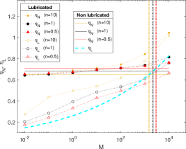
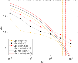
Figure 6: (a) The coefficients $\eta_{N},\eta_{L}$ of the similarity solutions at the vicinity of the fronts of the lubricated GC compared with the non-lubricated solutions, where $\mathscr{Q}=0.2,\mathscr{D}=0.1,\alpha=1$, $10^{-2}\leq\mathscr{M}\leq 10^{4}$, and $n=10,1,0.5$. The $\eta_{N}$ of the non-lubricated theory (solid lines) are independent of $\mathscr{M}$ and diminish with $n$, whereas those of the lubricated theory (solid markers at corresponding colors) are nearly equal in the liquid limit ($\mathscr{M}\ll 1$) and grow monotonically with $\mathscr{M}$. The corresponding $\eta_{L}$ of the non-lubricated theory (- - -, cyan) are independent of $n$, unlike those of the lubricated theory (hollow markers), but both grows monotonically with $\mathscr{M}$. Vertical grid lines mark the non-lubricated threshold viscosity ratio $\mathscr{M}_{c}$. (b) The difference $\Delta\eta\equiv\eta_{N}-\eta_{L}$ of the lubricated and non-lubricated values in panel a.

The intercept difference $\Delta\eta\equiv\eta_{N}-\eta_{L}$ predicted by the non-lubricated theory (49) diminishes with $\mathscr{M}$ and becomes negative when $\mathscr{M}$ grows beyond a threshold value that we denote by $\mathscr{M}_{c}$ (Figure 6b). This implies that across that threshold in the viscosity ratio $\eta_{L}>\eta_{N}$ and the lubricating front outstrips the upper fluid front. The threshold viscosity ratio $\mathscr{M}_{c}$ is found by setting $\Delta\eta=0$ and solving for $\mathscr{M}$

$$\mathscr{M}_{c}\equiv\left(\frac{2\pi}{\mathscr{Q}}\frac{9}{28}\right)^{3}\left(\frac{9(3\alpha+1)}{8\mathscr{D}}\right)\left[\frac{1+\mathscr{Q}}{2\pi}\frac{(5n+2)(3n+1)}{(2n+1)^{2}}N^{\textstyle{-\frac{n}{2n+1}}}\right]^{\textstyle{\frac{8(2n+1)}{5n+3}}}.$$ (50)

Therefore, in the purely Newtonian case the threshold viscosity ratio is

$$\mathscr{M}_{c}(n=1) = \frac{1}{\mathscr{D}}\left(1+\frac{1}{\mathscr{Q}}\right)^{3}$$ (51)

and is independent of $\alpha$. In the case of constant flux $\alpha=1$ the threshold is

$$\mathscr{M}_{c}(\alpha=1) = \left(\frac{2\pi}{\mathscr{Q}}\frac{9}{28}\right)^{3}\frac{9}{2\mathscr{D}}\left[\frac{1+\mathscr{Q}}{2\pi}\frac{(5n+2)(3n+1)}{(2n+1)^{2}}N^{\textstyle{-\frac{n}{2n+1}}}\right]^{\textstyle{\frac{8(2n+1)}{5n+3}}}.$$ (52)

This behaviour reasoned based on the non-lubricated theory is consistent with the trend implied from the numerical solution of the full lubricated theory (Figure 6b), though we do not explicitly observe an outstripping of the outer front by the inner one since the present simulation assumes $r_{L}<r_{N}$.

5.2 Exponent outstripping

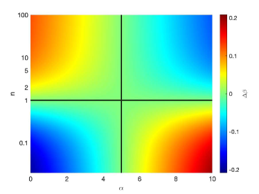
Figure 7: The exponent difference $\Delta\beta$ as a function of the fluid discharge exponent $\alpha$ and the viscosity exponent $n$. Dark lines are the $\Delta\beta=0$ contours, where global similarity solutions exist. When $\Delta\beta>0$ (hot colors) the lubricating fluid front $r_{L}$ outstrips the non-Newtonian fluid front $r_{N}$.

Another mechanism of outstripping can arise due to the different time exponents of the two fronts. This difference can be evaluated from the similarity solutions at the vicinity of each front. Specifically, denoting the front exponents by $\beta_{N}\equiv[\alpha(1+2n)+1]/(5n+3)$ (43a) and $\beta_{L}\equiv(3\alpha+1)/8$ (46a) then

$$\Delta\beta\equiv\beta_{L}-\beta_{N}=\frac{(5-\alpha)(n-1)}{8(5n+3)}.$$ (53)

When the flow has a global similarity solution ($\alpha=5$ or $n=1$) the exponents of the two fluid fronts are identical $\Delta\beta=0$, implying that asymptotically in time the gap between the two fronts evolves with the same exponent and the ratio of their position $r_{L}/r_{N}$ is constant. When $n\neq 1$ and $\alpha\neq 5$ there is no global similarity solution, implying that $\beta_{L}\neq\beta_{N}$ and that the fronts ratio evolves proportionally to $t^{\Delta\beta}$. Consequently, the gap between the fronts closes down in time and front outstripping occurs when $\Delta\beta>0$, which is when $\alpha<5~{}\&~{}n>1$ or when $\alpha>5~{}\&~{}n<1$ (Figure 7). When $\Delta\beta<0$ intercept outstripping can still occur at early time $(t/t_{L}\gtrsim 1)$ when $\mathscr{M}>\mathscr{M}_{c}$.

6 Solutions for constant-flux discharge $\alpha=1$

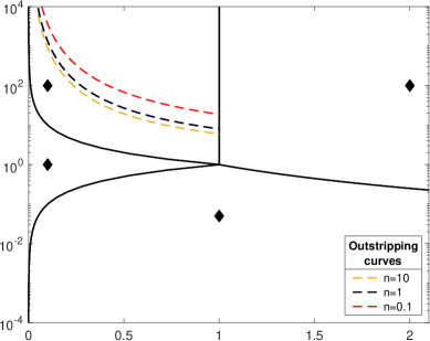
Figure 8: The $\mathscr{M}$ - $\mathscr{Q}$ state map for $\alpha=1$, $n=1$ and $\mathscr{D}=1$ is divided into four characteristic flow regimes I-IV. The dashed curves marks the critical viscosity ratios $\mathscr{M}_{c}(\mathscr{Q},n)$ (equation 52), beyond which we expect the front of the lubricating fluid to outstrip the front of the top fluid. The characteristic solution of the $\mathscr{M}-\mathscr{Q}$ states marked by diamonds are shown in Figure 9.

The case of constant flux ($\alpha=1$) was explored theoretically in several asymptotic limits, including the case of no lubrication (Huppert, 1982; Sayag & Worster, 2013) and the case where both fluids are Newtonian (Kowal & Worster, 2015). These cases are useful to validate our general solutions in several asymptotic limits and to elucidate the impact of lubrication when the upper fluid is non-Newtonian.

When the upper fluid is Newtonian $(n=1)$ the flow is self similar and can be classified into four different flow regimes in the $\mathscr{M}$-$\mathscr{Q}$ state space (Kowal & Worster, 2015), in which the radial distribution of the fluid thickness and the evolution of the fronts have unique qualitative characteristics (Figures 8, 9). When the upper fluid is non-Newtonian ($n\neq 1$), no global similarity solution arises for a constant-flux discharge (§2.3). Nevertheless, we find numerically that the characteristic distributions of the fluid thickness in each of the four regimes are qualitatively preserved (Figure 9). Moreover, the thickness of the lubricating fluid in the non-Newtonian case varies very weakly from that in the purely Newtonian case, and the fronts $r_{L}$ in both cases appear to follow a similar evolution pattern (Figure 9). In contrast, the propagation rate of the front $r_{N}$ varies strongly with the non-Newtonian properties of the upper fluid, becoming faster than the purely Newtonian case for shear-thickening fluids and slower than the purely Newtonian case for shear-thinning fluids (Figure 9). This pattern in all of the four regimes can be physically rationalised through a dimension-based argument: the radial velocity at constant flux $[u]\sim Q/(2\pi RH)$ combined with the thickness scale $[H]\sim(Q\mu_{\ell}/\rho g)^{1/4}$ (25c) implies that the dominant strain rate $[\p u/\p z]\sim Q/(2\pi RH^{2})\sim(\rho gQ/\mu_{\ell})^{1/2}/(2\pi R)$ declines radially. Consequently, a shear-thinning fluid ($n>1$) becomes increasingly more viscous with radius than a shear-thickening fluid, leading to its relatively slower propagation.

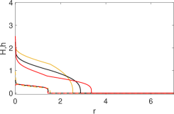
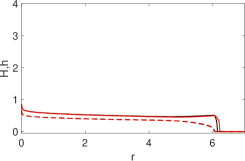
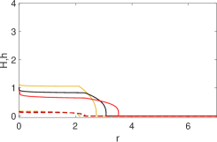
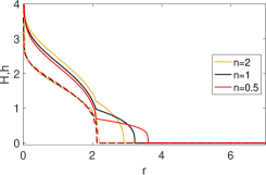
Figure 9: Characteristic solutions of each of the four states in the different regimes marked by $\blacklozenge$ in Figure 8 for a range of power-law exponents (yellow $n=2$, black $n=1$ and red $n=0.5$), at constant flux ($\alpha=1$), showing the position of the free surface of the lubricated power-law fluid (solid), and the lubricating Newtonian fluid (dash), at constant dimensionless time t=20, and $\mathscr{D}=1$.

The slower front speed of a shear-thinning fluid compared to a Newtonian fluid implies that outstripping by the front of the Newtonian lubricating fluid may occur after some time (§5). We investigate this more carefully by considering the evolution of the two fronts within a range of viscosity ratios $10^{-2}\leq\mathscr{M}\leq 10^{4}$, a range of fluid exponent $n=10,1,0.5$ and for fixed flux ratio $\mathscr{Q}=0.2$ and density ratio $\mathscr{D}=0.1$. Even though no global similarity solution of the first kind exists when $\alpha,n\neq 1$, we find that each front has a power-law evolution in time of the form

$$r_{N}(t)\approx c_{N}t^{\beta_{N}},\quad r_{L}(t)\approx c_{L}(t-1)^{\beta_{L}}$$ (54)

in dimensionless units, where we compute the intercepts $c_{N},c_{L}$ and the exponents $\beta_{N},\beta_{L}$, which may depend on the dimensionless groups $\mathscr{M},\mathscr{Q},\mathscr{D}$ and $n$, through regression to the numerical solution (Figures 10, 11, and 11). Our numerical solver does not admit front outstripping since it constrains $r_{L}\leq r_{N}$. Therefore, we infer that front outstripping is in progress when the interval $r_{N}-r_{L}$ is closing in time.

In the upper-fluid “liquid” limit, $\mathscr{M}\ll 1$, we find that the numerical solution for the front of the upper fluid evolves consistently with (42), in which $\beta_{N}=(2+2n)/(5n+3)$ and $c_{N}=\xi_{N}\mathscr{N}^{1/(5n+3)}$. For example, when $\mathscr{M}=0.01$ the computed exponents $\beta_{N}$ for $n=0.5,1,10$ differ from the corresponding theoretical values $6/11,1/2,22/53$ by less than 2% (Figure 10a). The larger discrepancy among those is for the shear-thinning fluid, which is expected due to the stronger coupling in this case between the upper and the lower fluid layers, as mentioned in §4.3.2. The corresponding intercepts $c_{N}$ differ by less than 5% from the theoretical values. The lubricating fluid front $r_{L}$ evolves with exponent $\beta_{L}\approx 1/2$ for $n=1$, larger than $1/2$ for a shear-thinning fluid (by 10% for $n=10$), and smaller than 1/2 for shear-thickening fluid (by 1.2% for $n=1/2$) (Figure 10a). The corresponding intercepts have small variation with $n$, being in the range $0.17\lesssim c_{L}\lesssim 0.21$, which is much smaller than the intercept in non-lubricated Newtonian GCs $\xi_{L}(1/3)^{1/8}\approx 0.62$.

In the upper-fluid “solid” limit, $M\gg 1$, we find that the front of the lubricating fluid evolves consistently with (40), in which $\beta_{L}\rightarrow 1/2$ is $n$-independent, and the solution for $\beta_{N}$ also tends to $1/2$ (Figure 10b). For intermediate $\mathscr{M}$ values we find that the front exponent $\beta_{N}$ varies weakly with $\mathscr{M}$ initially ($\mathscr{M}\lesssim 10$), remaining close to the $\mathscr{M}\ll 1$ asymptotic values (Figure 11a), and the intercept $c_{N}$ grows with $\mathscr{M}$ and varies weakly with $n$ (Figure 11d). The exponent of the lubricating front $\beta_{L}$ grows with $\mathscr{M}$ over 1/2 for shear-thickening fluids and less than 1/2 for shear-thinning fluids (Figure 11b), whereas the intercept $c_{L}$ grows monotonically with $\mathscr{M}$ for all $n$s while varying very weekly with $n$ (Figure 11e).

Throughout the range $10^{-2}\leq\mathscr{M}\leq 10^{4}$ we find that $\beta_{N}>\beta_{L}$ for shear-thickening ($n<1$), $\beta_{N}<\beta_{L}$ for shear-thinning fluids ($n>1$), and $\beta_{N}=\beta_{L}=1/2\pm 0.0008$ when $n=1$ (Figure 11c), consistently with our predictions of the similarity solutions near the front (§5.2). This implies that in the long-time limit the front $r_{L}$ outstrips $r_{N}$ when the upper fluid is shear thinning, independently of $\mathscr{M}$, while no exponent outstripping is expected when the upper fluid is shear thickening. However, the exponent differences $|\Delta\beta|\equiv|\beta_{L}-\beta_{N}|$ declines with $\mathscr{M}$ so that when $\mathscr{M}=10^{4}>\mathscr{M}_{c}$ it is marginally zero (Figure 11c), implying termination of the exponent-driven outstripping. Simultaneously, the intercept difference $c_{N}-c_{L}$ is positive throughout the range of $\mathscr{M}$ but approaches zero at the vicinity of $\mathscr{M}=10^{4}$ (Figure 11f). This may reflect the approach to an intercept-driven outstripping ($c_{N}-c_{L}<0$) across a critical viscosity ratio $\mathscr{M}>\mathscr{M}_{c}$, given by (52), while both exponents converge to $1/2$. We note again that numerically we do not resolve explicit outstripping, so the behaviour as $\mathscr{M}$ approaches $\mathscr{M}_{c}$ and grows beyond it reflects mostly the qualitative trend.

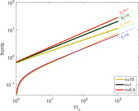
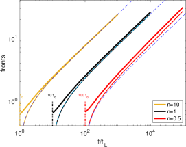
Figure 10: (a) The non-dimensional front positions $r_{N}$ (—, thick) and $r_{L}$ (—, thin) for varying power-law fluid exponents, $n=10,1,0.5$, and for dimensionless parameters $\alpha=1$, $\mathscr{Q}=0.2$ and $\mathscr{D}=0.1$. (a) $\mathscr{M}=0.01$. Shown for reference the theoretical prediction for $r_{N}(t)$ (eq. 42) in the $\mathscr{M}\ll 1$ limit (- - -, green), and with the prediction for the purely Newtonian solution (- - -, blue). (b) $\mathscr{M}=10^{4}>\mathscr{M}_{c}(n)$. Shown for reference curves with exponent 1/2 (—, blue), corresponding to the purely Newtonian solution. The exponents of each front are $\beta_{N}=0.4962\pm 0.0006,0.5\pm 0.001,0.523\pm 0.003$ and $\beta_{L}=0.4984\pm 0.0001,0.4998\pm 0.0003,0.526\pm 0.002$ for $n=10,1,0.5$, respectively.

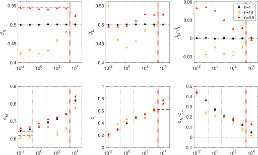
Figure 11: The fitted exponents and intercepts to numerical solutions of the fronts $r_{N},r_{L}$ for varying $\mathscr{M}$, and $n=10,1$ and $0.5$, for $\alpha=1$, $\mathscr{Q}=0.2$ and $\mathscr{D}=0.1$. Vertical grid line (dotted blue) marks the intercept-driven outstripping threshold $\mathscr{M}_{c}(n)$. (a) The exponent $\beta_{N}$. Horizontal grid lines show the predicted asymptotic ($\mathscr{M}\ll 1$) exponents $(2n+2)/(5n+3)$(eq. 42) corresponding by color to the specific $n$s. (b) The exponent $\beta_{L}$. Horizontal grid line show the predicted asymptotic ($n=1$) exponent $0.5$ (Kowal & Worster, 2015). (c) The exponent difference $\beta_{N}-\beta_{L}$. The differences in $\mathscr{M}=10^{4}$ are $-0.002\pm 0.001,0.0008\pm 0.003$, and $-0.003\pm 0.005$ for $n=10,1,0.5$, respectively. Horizontal grid lines represents the critical value for exponent outstripping. (d) The intercept $c_{N}$. Vertical grid lines (dash grey) mark the regime thresholds (Figure 8). Horizontal grid lines show the predicted asymptotic ($\mathscr{M}\ll 1$) intercepts $\xi_{N}\mathscr{N}^{1/(5n+3)}$ (eq. 42) corresponding by color to the specific $n$s. (e) The intercept $c_{L}$. Vertical grid lines (dash grey) mark the regime thresholds (Figure 8). Dashed grey curves are the theoretical prediction of $c_{L}$ for $n=1$ (Kowal & Worster, 2015). Horizontal grid line shows the asymptotic intercept of a non-lubricated Newtonian GC $\xi_{N}(1/3)^{1/8}$ (Huppert, 1982). (e) The intercept difference $c_{N}-c_{L}$. Horizontal grid lines mark the critical value for intercept outstripping.

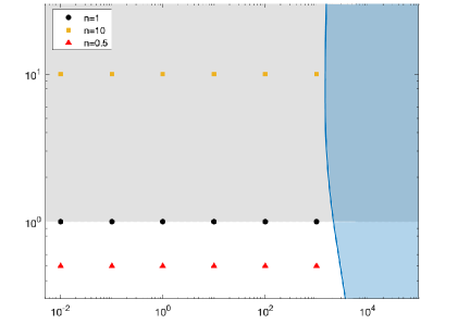
Figure 12: The $\mathscr{M}-n$ state map for $\alpha=1,\mathscr{Q}=0.2$, and $\mathscr{D}=0.1$, showing the numerical simulations presented in Figure 11 (markers). The region (cyan) bounded by the curve $\mathscr{M}_{c}(n)$ is where Intercept-driven outstripping occurs. The region (gray) bounded by $n=1$ is where exponent-driven outstripping occurs.

7 Comparison with experimental evidence for $\alpha=1$ and $n>1$

The theory we have developed can be validated with the recent laboratory experiments of lubricated GCs at constant-flux ($\alpha=1$) that consisted of a strain-rate softening fluid that was lubricated by a denser Newtonian fluid (Kumar et al., 2021). The experimental findings have shown that for flux ratio $\mathscr{Q}\lesssim 0.06$ both fronts were highly axisymmetric, in experiments that lasted over $10t_{L}$ in some cases, implying that a comparison with our axisymmetric theory should be valid.

7.1 Proparation of the fronts

Experimentally it was found that the two fronts evolved faster than those of non-lubricated GCs of the corresponding fluids. Nevertheless, each front had a power-law time evolution with a similar exponent as non-lubricated GCs of the corresponding fluids. In particular, the front $r_{N}$ evolved with exponent $(2n+2)/(5n+3)$ before the lubrication fluid was introduced ($t\leq t_{L}$) as well as when $t\gtrsim 5t_{L}$, while the exponent was larger during the transition between the two intervals. At the same time, the front $r_{L}$ evolved with exponent 1/2.

To compare our theoretical predictions to the experimental measurements we compute numerical solutions to each of the 15 experiments described in Kumar et al. (2021, Table 2c and eq. 2.2) (Figures 13, 14) based on the measured quantities $\mathscr{Q},\mathscr{M},\mathscr{D}$ and $n$ and without any fitting parameter. The viscosity ratio in each of these experiments was in the range $1\ll\mathscr{M}<\mathscr{M}_{c}$, implying that the experiments were all in the exponent-outstripping regime (§5.2) as well as in the solid-limit regime (§4.3.1). Consequently, we expect the lubrication front to evolve like $r_{L}\propto t^{1/2}$.

Comparing the time exponents, we find that the numerical solutions and the theoretical predictions are consistent with those measured experimentally for both $r_{N}$ (Figure 13a, b) and $r_{L}$ (Figure 14a, b). Specifically, during $t_{L}<t\lesssim 5t_{L}$ the solutions to the front $r_{N}$ evolve with larger exponent than non-lubricated current (Figure 13a,b), and when $t\gtrsim 5t_{L}$ the exponent diminishes and converges back to that of non-lubricated GCs (Figure 13b). Similarly, the solutions to the front $r_{L}$ evolve with an exponent 1/2, consistently with the experimental measurements (Figure 14a, b). In spite of the exponent consistency between the experiment and the theory, the experimental fronts advance faster than the predicted ones (Figure 13c, d and 14c, d). This discrepancy is larger in experiments with higher polymer concentration (Figure 13d and 14d). It implies that the numerically predicted intercepts are lower than those that were measured experimentally, suggesting that additional physical processes that contribute to a faster front propagation are not accounted for by our theoretical model. We elaborate on potential additional mechanisms in §8.

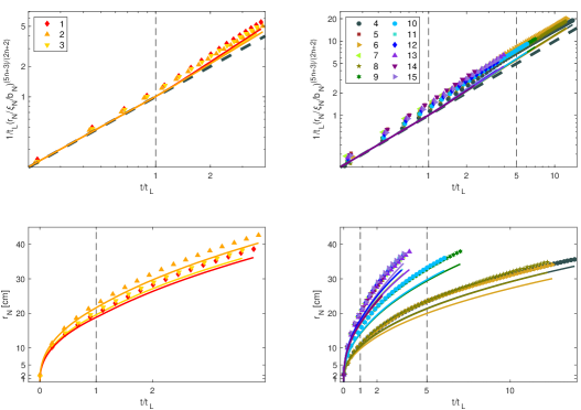
Figure 13: Comparison of the theoretical predictions of the fronts $r_{N}$ evolution (colored lines) with the experimental measurements (markers) (Kumar et al., 2021, experiments #1-15 in table 2c). (a, c) Comparison with the 1% polymer concentration (experiments 1-3) in linear and log scale respectively. In panel (a) the fronts are normalised with the similarity solution of non-lubricated GCs of power-law fluids (Sayag & Worster, 2013) and the front solution of such curent is shown for reference (dash, gray). (b, d) Same as panels a and c but for experiments (4-15) of the 2% polymer concentration.

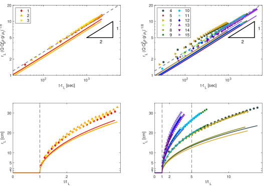
Figure 14: Comparison of the theoretical predictions of the fronts $r_{L}$ evolution (colored lines) with the experimental measurements (markers) (Kumar et al., 2021, experiments #1-15 in table 2c). (a-b) Comparison with the 1% polymer concentration (experiments 1-3) in linear and log scale respectively. In panel (b) the fronts are normalised with the similarity solution of a Newtonian lubricated GCs (Kowal & Worster, 2015) and the front solution of such a current is shown for reference (dash, gray), with a fitted coefficient 0.27. (c-d) Same as panels a and b but for experiments (4-15) of the 2% polymer concentration.

7.2 Thickness evolution

Experimentally, the thickness of the lubricated, non-Newtonian fluid was found to be nearly uniform in the lubricated region. The layer of the lubricating fluid was also largely uniform with localised spikes, and its average thickness was approximated through mass conservation to be $h_{\ell}=Q_{\ell}(t-t_{L})/\rho_{\ell}\pi r_{L}^{2}$ (Kumar et al., 2021). This nearly uniform pattern differs substantially from the monotonically diminishing thickness of a non-lubricated GC under similar conditions. Our numerical solutions, which do not involve any fitting parameter, follow a similar pattern as in the experiments (Figure 15). The theoretical and experimental patterns are highly consistent during most of the flow (e.g., Figure 15a-c), but discrepancy between the two grows progressively near the fronts $r_{L},r_{N}$ and in the non-lubricated region (e.g., Figure 15d). In particular, the fronts in the experiment evolve faster than those computed numerically, and the thickness distribution of the top fluid at the vicinity of the lubricating front changes more sharply in the computed solutions than in the measurements. This growing discrepancy may imply the action of additional mechanisms, as we elaborate in §8.

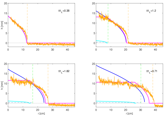
Figure 15: The thickness field of the top fluid layer along a radius at four different times during the non-lubricated phase (a) and during the lubricated phase (b-d). The experimental thickness measurement derived from transmitted-light intensity (—, orange) (Kumar et al., 2021, experiment #1 in table 2c) compared with the corresponding solution (Sayag & Worster, 2013) for the thickness of a non-lubricated GC of PL fluid (—, blue) and with the numerical solution for lubricated power-law fluid (—, magenta). Also shown are the corresponding numerical solution for the lubrication layer (—, cyan), and the experimentally measured fronts $r_{N}$ (vertical grid line, orange), $r_{L}$ (vertical grid line, green), and the average thickness of the lubrication fluid $h_{\ell}$ (- - -, pale blue).

8 Discussion

The lubricated GCs that we consider involve five dimensionless parameters $\mathscr{Q},\mathscr{D},\mathscr{M},n$ and $\alpha$, associated with significant qualitative transitions in the structure of the solution, in the relative motion of the fluid fronts and their stability, and in the thickness distribution of the two fluids.

The fluid exponent $n$ and the discharge exponent $\alpha$ have a dramatic qualitative impact on the solutions. Specifically, similarity solutions exist only when $n=1$, in which both fluids follow a similar constitutive law, and when $\alpha=5$. In those cases the two fronts evolve with the same power law in time and as a result the ratio $r_{N}/r_{L}$ is constant. In all other cases ($n\neq 1,\alpha\neq 5$) the fronts also appear to follow a power law evolution, but each with a different exponent, implying that asymptotically in time the ratio $r_{N}/r_{L}$ evolves following a power law in time with exponent $\Delta\beta$ (53). Therefore, there are solutions where $r_{N}/r_{L}$ declines in time resulting in the lubrication front outstripping the front of the upper fluid ($n>1~{}\&~{}\alpha<5$, and $n<1~{}\&~{}\alpha>5$), and otherwise $r_{N}/r_{L}$ grows in time (Figure 7).

The flux ratio $\mathscr{Q}$ can lead to the emergence of two significantly different patterns, and may have a critical impact on the front stability. When $\mathscr{Q}<1$ the flux of the lubricating fluid is lower than the top fluid layer. Consequently, the thickness of the lubricating layer is significantly smaller and the propagation of the front $r_{L}$ is affected by the relatively larger pressure imposed by the thicker top layer (Figure 9III, and Figure 15). The opposite occurs when $\mathscr{Q}>1$ – the lubricating fluid is discharged at a larger flux and its thickness is significantly larger than the top fluid layer (Figure 9II). $\mathscr{Q}$ may also have a crucial impact on the stability of the axisymmetric fronts. Preliminary experimental evidence indicate that when the flux is constant ($\alpha=1$), the top fluid layer is strain-rate softening ($n=6$) and $\mathscr{M}\gg 1$, the initially axisymmetric fronts become unstable when $\mathscr{Q}\gtrsim 0.1$ and develop fingering patterns after an initial axisymmetric spreading (Kumar et al., 2021). Similar symmetry breaking also emerges in the purely Newtonian case when $0.14\lesssim\mathscr{Q}\lesssim 0.44$ (Kowal & Worster, 2015).

The viscosity ratio $\mathscr{M}$ affects the relative motion of the fronts, and the relative thickness of the fluid layers. At a high viscosity ratio ($\mathscr{M}\gg 1$) the more viscous top fluid is effectively solid-like compared with the less viscous lower fluid. Consequently, the flow in the lubricated region is independent of the fluid exponent $n$, and both fluid layers in that region follow the same similarity solution, in which the front of the lubrication fluid $r_{L}$ evolves with a time exponent $(3\alpha+1)/8$, same as a non-lubricated Newtonian GC (40). In the low viscosity ratio ($\mathscr{M}\ll 1$) the top fluid is significantly more mobile than the lower fluid layer, which does not provide an effective lubrication. In this case the two fluid layers in the lubricated region do not exhibit a global similarity solution, but the top fluid layer along the whole domain does. Consequently, a self-similar solution exist in the top-fluid layer, in which the front $r_{N}$ evolves with a time exponent $[\alpha(2n+1)+1]/(5n+3)$, same as a non-lubricated GCs (42). The impact of the viscosity ratio on the fluid thickness distributions can be appreciated through the constant flux case ($\alpha=1$), in which the free surface of the top fluid is substantially flatter in the $\mathscr{M}\gg 1$ case than in the $\mathscr{M}\lesssim 1$ case (Figure 9).

Independently of the value of the dimensionless parameters, the solutions at the vicinity of the fronts are also self similar, with exponents consistent with those of non-lubricated GCs of power-law fluids (Huppert, 1982; Sayag & Worster, 2013). Particularly, both fronts evolve with an exponent $[\alpha(2n+1)+1]/(5n+3)$, which simplifies to $(3\alpha+1)/8$ for the Newtonian lubricating fluid. The intercepts of the fronts depend on the different dimensionless numbers of the system. Together, the exponents and the intercepts provide insights into the interaction between the two fronts. One important consequence of that interaction is the outstripping of the upper fluid front by the lower lubricating fluid front, which can occur either through the intercept difference $\Delta\eta$ or through the exponent difference $\Delta\beta$. The condition for an intercept-driven outstripping can be formalised in terms of the critical viscosity ratio $\mathscr{M}_{c}(\mathscr{Q},\mathscr{D},\alpha,n)$ (51), so that outstripping occurs when $\mathscr{M}>\mathscr{M}_{c}$. Physically this implies that when $\mathscr{Q}\ll 1$ then $\mathscr{M}_{c}\propto 1/\mathscr{Q}^{3}\gg 1$ and the top fluid should be significantly more viscous than the lower fluid for outstripping to occur, in which case the top fluid deforms substantially slower making it easier for the lubricating fluid front to outstrip. Alternatively, when $\mathscr{Q}\gg 1$ then for shear-thinning fluids $\mathscr{M}_{c}(n\rightarrow\infty)\propto\mathscr{Q}^{1/5}\gg 1$, whereas for shear-thickening fluids $\mathscr{M}_{c}(n\rightarrow 0)\propto 1/\mathscr{Q}^{1/3}\ll 1$. In either case the superiority of the lubricating fluid flux leads to front outstripping. When $\mathscr{M}<\mathscr{M}_{c}$ then $\Delta\eta>0$ and outstripping can only be driven by the exponent difference. As discussed above, the condition for that mechanism depends on the values of $n$ and $\alpha$ (Figure 7). For example, shear-thinning fluids at relatively low discharge exponent $(\alpha<5)$ become increasingly more viscous as they expand radially, resulting in slower front velocity than the lubricating fluid front. Moreover, their thickness and correspondingly the pressure they apply on the lubricating fluid is relatively larger and contribute further to the radial spreading of the lubricating fluid. We find that the intercept-driven outstripping can occur significantly faster than exponent-driven outstripping. For example, as in the constant flux ($\alpha=1$) case intercept-driven outstripping occurs at roughly $t/t_{L}\lesssim 10$, which is much faster than the $t/t_{L}\gtrsim 10^{3}$ in the exponent-driven case (Figure 10).

It is important to note that the global similarity solution that we find for a discharge exponent $\alpha=5$ arises in additional axisymmetric GCs of different settings, which a priori appear remotely related. This includes for example, isothermal lava domes that are modeled as axisymmetric GCs of visco-plastic fluids (Balmforth et al., 2000). The structure of the similarity solution in that case is identical to the lubricating GCs that we consider, in which the front evolves like $r\propto t^{2}$ and the fluid thickness evolves like $h\propto t$ independently of the fluid exponent $n$. Another system with a similarity solution at $\alpha=5$ is the axisymmetric viscous GCs flowing over a porous medium (Spannuth et al., 2009). Such a similarity among a broad range of physical systems may not be coincidental and could imply a more general symmetry associated with the circular geometry.

Many aspects of the theory were found consistent with experiments performed for the dimensionless parameters $\mathscr{D}\approx 0.15,\mathscr{Q}<0.06,1\ll\mathscr{M}<\mathscr{M}_{c},\alpha=1$, and $n>1$ (Kumar et al., 2021). In particular, the time evolution of both fluid fronts predicted by the theory is consistent with the power law measured in the experiments. In addition, the thickness distribution we predict for the top fluid layer is in good agreement with the experimental measurements. However, some discrepancies that arise may imply that the theory is not entirely complete. Specifically, the theoretical predictions for the intercepts do not accurately capture the measured ones, particularly in the case of the lubricating front, which evolves faster than the theoretical predictions. Several potential physical mechanisms that the present theory does not account for may explain these discrepancies. One possible mechanism is that the lubrication front $r_{L}$ advances as a hydrofracture in between the substrate and the relatively solid viscous fluid layer (Ball & Neufeld, 2018), or as a shock in the fluid-fluid interface at $r_{L}$ (Dauck et al., 2019). In addition, discrepancy between the experimental measurements of $r_{N}$ before introducing the lubrication fluid ($t/t_{L}<1$) and the theoretical prediction of a non-lubricated GC, particularly for the 2% polymer concentration (Kumar et al., 2021), may imply that the power-law constitutive equation that we use is incomplete. Specifically, the time for the viscosity to adjust to the evolving strain rates may not be instantaneous as we assume, but finite. In addition polymer entanglements may arise in higher polymer concentrations that potentially drive wall slip at the fluid-solid interface through adhesive failure of the polymer chains at the solid surface or through cohesive failure owing to disantanglement of chains in the bulk from chains adsorbed at the wall (Brochard & Gennes, 1992). The implications of these potential physical mechanisms will be addressed in future studies.

9 Conclusions

Lubricated gravity currents are controlled by complex interactions between two fluid layers. The lower lubricating layer modifies the friction between the substrate and the top layer, which in turn applies stresses that affect the distribution of the lubricating layer. The resulting flow can vary dramatically from non-lubricated gravity currents.

Unlike previous axisymmetric gravity current models that involve a single fluid layer (Huppert, 1982; Sayag & Worster, 2013), or two coupled layers that have the same constitutive structure (Kowal & Worster, 2015), the flow we consider does not in general admit a global self-similar solution. Exceptional cases, in which the model has a global similarity solutions are the purely Newtonian case and the case of a discharge exponent $\alpha=5$. Several other situations admit a similarity solution in part of the domain. This includes the asymptotic limits of the viscosity ratio, corresponding to the top layer solid ($\mathscr{M}\gg 1$) and liquid ($\mathscr{M}\ll 1$) limits, and the solution at the vicinity of the fluid fronts. The latter implies that the time evolution of each front is proportional to that of the non-lubricated front of the corresponding fluid. This implies that generally the ratio of the two fronts positions $r_{N}/r_{L}$ either diverge in time or converge to zero, and that the difference of the front intercepts can change sign. Consequently, there are situations where the lubricating fluid front can outstrip the outer-fluid front. This situation can arise when the top fluid is non-Newtonian, having a different exponent than the lubricating fluid, but also when there is global similarity and the viscosity ratio is larger than a critical value $\mathscr{M}_{c}$ that depends on the fluids flux and density ratios, on the discharge exponent and on the power-law fluid exponent. In the canonical case of constant flux the flow we consider has no global similarity when the top fluid is non-Newtonian. The evolution of the lubricating front does not differ substantially from the purely Newtonian case, but the evolution of the top fluid front differs substantially. Our model solutions are found consistent with laboratory experiments (Kumar et al., 2021), particularly in predicting the time exponents of the front evolution and the thickness fields. Discrepancies that we find in the intercepts predictions, particularly that of the lubricating fluid front, suggest that additional physical mechanisms may contribute to the front evolution, such as hydrofracturing or wall-slip along the substrate. Exploration of these mechanisms will be the topic of future studies. Our results have implications to the understanding of spatiotemporal distribution of lubrication networks beneath ice sheets and to understanding their stability.

AG was partially supported by VATAT High-TEC fellowship for excellent women in science. This research was supported by the GERMAN-ISRAELI FOUNDATION (grant No. I240430182015). Declaration of Interests. The authors report no conflict of interest.

Appendix A Validation of the numerical code

A.1 Non-lubricated gravity currents

\begin{overpic}[scale={0.45}]{figsR/fBall.pdf} \put(58.7,19.5){\includegraphics[scale={0.089}]{figsR/figAPXallSW}} \end{overpic}

Figure 16: Validation of the lubricated GC numerical solution with the theoretical prediction of non-lubricated GC of power-law fluids ($\mathscr{Q}=0,\alpha=1$) (Sayag & Worster, 2013). (a) Fluid height for n=5 at non-dimensional times t=1,4,7,10 in the regular thickness-radius space, and (b) in the thickness-radius space normalised by the theoretical prediction (c) Fluid height for n=5, 1 and 0.8, at non-dimensional time t=3. (d) The front $r_{N}(t)$ (solid), and the theoretical prediction for n=5, 1 and 0.8 (dash). (inset) Regression results to the slope (exponent) of the numerical solution for $n=1$ as a function of spatial resolution in the range 200-2400 points in logarithmic spaced mesh. Error bars represent the root-mean-square deviation of the fitted curve to the fronts.

The model we develop in §2 describes in the limit $\mathscr{Q}=0$ a non-lubricated GC that propagates under no-slip condition along the substrate. Such flow is similar to the flow in the non-lubricated region, and is known to have a similarity solution (Sayag & Worster, 2013)

$$h(r,t)\propto t^{\frac{n-1}{5n+3}},\qquad r_{N}(t)\propto t^{\frac{2n+2}{5n+3}},$$ (55)

for constant flux $\alpha=1$. We use this solution to validate our numerical solution in the $\mathscr{Q}=0$ limit. Specifically, we solve the dimensionless equation set (§2.3) with $\mathscr{Q}=0$, zero initial thickness $H(r,0)=0$, and logarithmically spaced spatial mesh with 1200 points. We find our solutions for the fluid height and for the leading front consistent with the theoretical predictions (Figure 16). Repeating the same computation for varying spatial resolutions, we find that the convergence accuracy of the front exponent to the predicted theoretical value grows with a the number of spatial grid points (Figure 16d, inset).

A.2 Lubricated Newtonian gravity currents

In the limit $n=1,\alpha=1$ our numerical model converges to the purely Newtonian lubricated GC discharged at constant flux (Kowal & Worster, 2015). Considering first the specific case where $\mathscr{M}=10000$, $\mathscr{Q}=0.2$ and $\mathscr{D}=0.1$, we find that both the fronts $r_{N},r_{L}$ and the upper fluid height at the lubricant front $H(r_{L})$ converge to the theoretical values $\eta_{N},\eta_{L}$ and $F(\eta)$, respectively (Figure 17). Second, we find that our solutions for the coefficients $\eta_{N}$ and $\eta_{L}$ is consistent with the theoretical predictions for a wide range of $\mathscr{M}$ values (Figures 11. As shown in Appendix A.1, small discrepancies from the predicted values are due to low spatial resolution. Lastly, the solutions to the specific regime discussed in §6 (Figures 9) is another evidence for the consistency between our numerical results and those of (Kowal & Worster, 2015, Figure 13).

Figure 17: Validation of the lubricated GC numerical solution with the Newtonian ($n=1$) lubricated GC (blue) with $\mathscr{M}=10,000$, $\mathscr{Q}=0.2$ and $\mathscr{D}=0.1$, showing the convergence of the normalized fronts (top) and the lubricated fluid height at lubricating fluid front, $r_{L}$ (bottom) to the theoretically predicted constant values (black).

References

- Ball & Neufeld (2018) Ball, T. V. & Neufeld, J. A. 2018 Static and dynamic fluid-driven fracturing of adhered elastica. Phys. Rev. F 3 (7).
- Balmforth et al. (2000) Balmforth, N. J., Burbidge, A. S., Craster, R. V., Salzig, J. & Shen, A. 2000 Visco-plastic models of isothermal lava domes. J. Fluid Mech. 403, 37–65.
- Brochard & Gennes (1992) Brochard, F. & Gennes, P. G. De 1992 Shear-dependent slippage at a polymer/solid interface. Langmuir 8 (12), 3033–3037.
- Daniel et al. (2017) Daniel, D., Timonen, J. V. I., Li, R., Velling, S. J. & Aizenberg, J. 2017 Oleoplaning droplets on lubricated surfaces. Nature Physics 13 (10), 1020–1025.
- Dauck et al. (2019) Dauck, T. F., Box, F., Gell, L., Neufeld, J. A. & Lister, J. R. 2019 Shock formation in two-layer equal-density viscous gravity currents. J. Fluid Mech. 863, 730–756.
- DeConto & Pollard (2016) DeConto, R. M. & Pollard, D. 2016 Contribution of Antarctica to past and future sea-level rise. Nature 531 (7596), 591–597.
- Fowler (1981) Fowler, A. C. 1981 A theoretical treatment of the sliding of glaciers in the absense of cavitation. Philosophical Transactions of the Royal Society of London. Series A, Mathematical and Physical Sciences 298 (1445), 637–681.
- Fowler (1987) Fowler, A. C. 1987 A theory of glacier surges. J. Geophys. Res. 92 (B9), 9111–9120.
- Glen (1952) Glen, J. W. 1952 Experiments on the deformation of ice. J. Glaciol. 2 (12), 111–114.
- Griffiths (2000) Griffiths, R. W. 2000 The dynamics of lava flows. Ann. Rev. Fluid Mech. 32, 477–518.
- Huppert (1982) Huppert, H. E. 1982 The propagation of two-dimensional and axisymmetric viscous gravity currents over a rigid horizontal surface. J. Fluid Mech. 121, 43–58.
- Keiser et al. (2017) Keiser, A., Keiser, L., Clanet, C. & Quéré, D. 2017 Drop friction on liquid-infused materials. Soft Matter 13 (39), 6981–6987.
- Kivelson et al. (2000) Kivelson, M. G., Khurana, K. K., Russell, C. T., Volwerk, M., Walker, R. J. & Zimmer, C. 2000 Galileo magnetometer measurements: A stronger case for a subsurface ocean at Europa. Science 289 (5483), 1340–1343.
- Kowal & Worster (2015) Kowal, K. N. & Worster, M. G. 2015 Lubricated viscous gravity currents. J. Fluid Mech. 766, 626–655.
- Kowal & Worster (2019a) Kowal, K. N. & Worster, M. G. 2019a Stability of lubricated viscous gravity currents. part 1. internal and frontal analyses and stabilisation by horizontal shear. J. Fluid Mech. 871, 970–1006.
- Kowal & Worster (2019b) Kowal, K. N. & Worster, M. G. 2019b Stability of lubricated viscous gravity currents. part 2. global analysis and stabilisation by buoyancy forces. J. Fluid Mech. 871, 1007–1027.
- Kumar et al. (2021) Kumar, P., Zuri, S., Kogan, D., Gottlieb, M. & Sayag, R. 2021 Lubricated gravity currents of power-law fluids. Journal of Fluid Mechanics 916.
- Kyrke-Smith et al. (2013) Kyrke-Smith, T. M., Katz, R. F. & Fowler, A. C. 2013 Subglacial hydrology and the formation of ice streams. Proc. R. Soc. A p. 30494.
- Lister & Kerr (1989) Lister, J. R. & Kerr, R. C. 1989 The propagation of two-dimensional and axisymmetric viscous gravity currents at a fluid interface. J. Fluid Mech. 203, 215–249.
- Pegler & Worster (2012) Pegler, S. S. & Worster, M. G. 2012 Dynamics of a viscous layer flowing radially over an inviscid ocean. J. Fluid Mech. 696 (-1), 152–174.
- Sayag & Worster (2013) Sayag, R. & Worster, M. G. 2013 Axisymmetric gravity currents of power-law fluids over a rigid horizontal surface. J. Fluid Mech. 716, 716 R5–1–716 R5–11.
- Sayag & Worster (2019) Sayag, R. & Worster, M. G. 2019 Instability of radially spreading extensional flows. Part 1. Experimental analysis. J. Fluid Mech. 881, 722–738.
- Schoof & Hewitt (2013) Schoof, C. & Hewitt, I. 2013 Ice-Sheet Dynamics. Ann. Rev. Fluid Mech. 45 (1), 217–239.
- Spannuth et al. (2009) Spannuth, M J, Neufeld, J A, Wettlaufer, J S & Worster, M G 2009 Axisymmetric viscous gravity currents flowing over a porous medium. J. Fluid Mech. 622, 135–144.
- Stokes et al. (2007) Stokes, C. R., Clark, C. D., Lian, O. B. & Tulaczyk, S. 2007 Ice stream sticky spots: A review of their identification and influence beneath contemporary and palaeo-ice streams. Earth-Science Rev. 81 (3-4), 217–249.
- Woods & Mason (2000) Woods, A. W. & Mason, R. 2000 The dynamics of two-layer gravity-driven flows in permeable rock. J. Fluid Mech. 421, 83–114.