SM:Decoding the DC and optical conductivities of disordered MoS₂ films: an inverse problem

I Interpolation Method for CA

To demonstrate the agreement between minimizing concentration of $\chi$ and the actual disorder concentration the configurationally averaged (CA) conductance is expanded to linear order in $n$ as datta_1995

$$\langle\Gamma(E,n)\rangle=\Gamma_{0}(E)-\beta(E)\,n,$$ (1)

where $\beta(E)$ is the derivative of $\langle\Gamma(E,n)\rangle$ with respect to $n$ evaluated at $n=0$.

Satisfactory accuracy levels of the inversion method relies on carrying out the CA part of the calculation with a good resolution in terms of $n$ but the computational costs of doing so with a large number of concentration points by brute force is substantial. The approximation in Eq.1 provides a doorway to generate CA for more values of $n$ using interpolation supported by machine learning. Fig. 1 shows a misfit function generated using numerical (red) and interpolated (black) data. This model studies the CA data (CA corresponding to red points) to generate CA spectrum for different values of $n$ (corresponding to black points). Eq.1 is valid for a small range of concentration but it starts to move away from the linear nature as disorder concentration increases. This results in failure to understand the caveats of CA spectrum.

Machine Learning (ML) becomes a very handy tool in order to generate CA conductance spectrum. It computes CA spectrum without losing details of the conductance quantum signatures and at a low computational costs. Fig. 2 shows very good prediction of CA optical spectrum corresponding to 8% disorder with numerically calculated optical spectrum in blue. 7 datasets corresponding to different concentrations of numerically calculated CA spectrum were used to train the model. Same model is used to generate rest of the CA points shown in black in Fig. 1.

Wolfram Mathematica provides predefined ML tools called Predict and Classify to define a model. Both tools can generate the output corresponding to concentration and energy in this case. Model uses numerically computed CA spectrums as the training examples. Spectrum provides large number energy points to train the model. It is worth pointing out that while more sophisticated ML techniques are available to model quantum transport machine_learning_interpolation ; machinelearning_modelling , this is by no means an essential ingredient of this inversion method but one that can speed up the inversion and improve its accuracy.

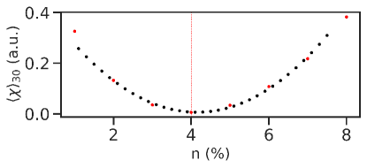
Figure 1: Misfit function for the machine learning optical conductivity interpolated data (black) and for the numerical data (red). The model still predicts the minimum correctly while providing more resolution around it, allowing for fine probing different parent configuration concentrations with lower computational cost.

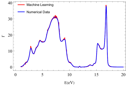
Figure 2: Configurational average corresponding to 8% disorder randomly distributed in the device represented in Blue. In Red, ML optical conductivity shows very good prediction with the numerical result.

II MoS₂ Band Structure and conductivity for clean systems

Fig. 3(a) shows the comparison between the band structure calculations for MoS₂ obtained by DFT and by the effective tight-binding Hamiltonian taking into account 13 orbitals per unit cell. We have considered all hopping integrals with energies higher than 0.0125 of the maximum hopping value. Fig. 3(b) presents the density of states and the conductivity without disorder, both calculated with the kernel polynomial method for the effective tight-binding Hamiltonian. Fig. 4 show the optical conductivity pristine case.

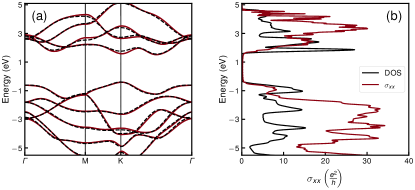
Figure 3: (a)Comparison between the band structures of a MoS₂ monolayer calculated without SOC employing DFT (solid line) and the effective tight-binding model (dashed line). (b) Density of states (black) and conductivity (blue) of MoS₂ calculated with KPM and the effective tight-binding model.

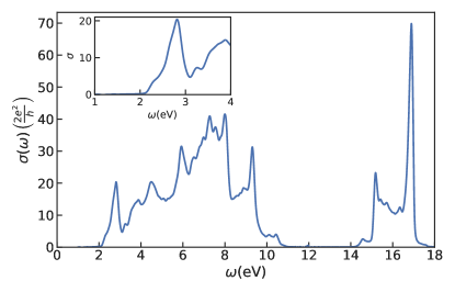
Figure 4: Optical conductivity of MoS₂ calculated with KPM and the effective tight-binding model with Fermi energy at 0 eV.

References

- (1) Supriyo Datta. Electronic Transport in Mesoscopic Systems. Cambridge University Press, Cambridge, 1995.
- (2) A. Mikhailiuk and A. Faul. Deep learning applied to seismic data interpolation. 2018(1):1–5, 2018.
- (3) Alejandro Lopez-Bezanilla and O. Anatole von Lilienfeld. Modeling electronic quantum transport with machine learning. Phys. Rev. B, 89:235411, Jun 2014.