In-medium screening effects for the Galactic halo and solar-reflected
dark matter detection in semiconductor targets

Abstract

Recently, the importance of the electronic many-body effect in the dark matter (DM) detection has been recognized and a coherent formulation of the DM-electron scattering in terms of the dielectric response of the target material has been well established in literatures. In this paper, we put relevant formulas into practical density functional theory (DFT) estimation of the excitation event rates for the diamond and silicon semiconductor targets. Moreover, we compare the event rates calculated from the energy loss functions with and without the local field effects. For a consistency check of this numerical method, we also compare the differential spectrum and detection reach of the silicon target with those computed with the $\mathtt{GPAW}$ code. It turns out that these DFT approaches are quite consistent and robust. As an interesting extension, we also investigate the in-medium effect on the detection of the solar-reflected DM flux in silicon-based detectors, where the screening effect is found to be less remarkable than on detection of the Galactic DM, due to the high energies of the reflected DM particles.

I Introduction

In recent years, both theorists and experimentalists begin to shift their focus on other directions beyond the weakly interacting massive particles (WIMPs). The sub-GeV dark matter (DM) as an alternative candidate, has attracted increasing attention for its theoretical motivations and detection feasibility. In the sub-GeV DM paradigm, the DM particles are expected to reveal itself via the weak DM-electron interaction in silicon- and germanium-based semiconductors (e.g., SENSEI (Barak:2020fql, ), DAMIC (Castello-Mor:2020jhd, ), SuperCDMS (Amaral:2020ryn, ), and EDELWEISS (Arnaud:2020svb, )) with energy thresholds as low as a few eV. In the theoretical aspect, since the appearance of the first estimation of the electronic excitation rates based on the first-principles density functional theory (DFT) (Essig:2015cda, ), similar investigations have been generalized to a wider range of target materials (Hochberg:2015pha, ; Essig:2016crl, ; Hochberg:2016ntt, ; Hochberg:2016sqx, ; Derenzo:2016fse, ; Hochberg:2017wce, ; Kadribasic:2017obi, ; Budnik:2017sbu, ; Knapen2018, ; Griffin:2018bjn, ; Griffin:2019mvc, ; Trickle:2019ovy, ; Kurinsky:2019pgb, ; Trickle:2019nya, ; Campbell-Deem:2019hdx, ; Coskuner:2019odd, ; Geilhufe:2019ndy, ; Griffin:2020lgd, ), and have spurred further discussions on the methodology (Liang:2018bdb, ; Kurinsky:2020dpb, ; Kozaczuk:2020uzb, ; Griffin:2021znd, ; Hochberg:2021pkt, ; Knapen:2021run, ), and extensive interpretations of the DM-electron interactions (Baxter:2019pnz, ; Emken:2019tni, ; Essig:2019xkx, ; Heikinheimo:2019lwg, ; Trickle:2020oki, ; Andersson:2020uwc, ; Su:2020zny, ; Catena:2021qsr, ).

Recently, nontrivial collective behavior of the electrons in solid detectors has also attracted attention (Kurinsky:2020dpb, ; Gelmini_2020, ; Kozaczuk:2020uzb, ; Knapen:2020aky, ; Liang:2020ryg, ; Mitridate:2021ctr, ). The related physics such as screening and the plasmon excitation that cannot be explained in terms of standard two-body scattering, and non-interacting single-particle states, can be well described with the dielectric function. The in-medium effect induced by the DM-electron interaction has been thoroughly investigated in Refs. (Knapen:2021run, ; Hochberg:2021pkt, ). In this work we also touch on this topic. Our first purpose is to provide a detailed derivation of the the DM-electron excitation event rate in the context of the linear response theory, and then calculate the excitation event rates for diamond and silicon targets using the DFT approach. We begin with the well-established description of the electron energy loss spectroscopy (EELS) in the homogeneous electron gas (HEG), and generalize the description to the crystalline environments, and finally to the case of DM-electron excitation process in semiconductor targets.

As is well known, the key quantity in describing the in-medium effect in EELS and DM-electron excitation process is the energy loss function (ELF), which is defined as the imaginary part of the inverse dielectric function $\mathrm{Im}\left[-1/\epsilon\left(\mathbf{Q},\omega\right)\right]$ for the HEG, with $\mathbf{Q}$ being the momentum and $\omega$ being the energy transferred to the electrons from the impinging particle. However, for the crystal targets, the ELF is generalized accordingly to the matrix form $\mathrm{Im}\left[\epsilon_{\mathbf{G},\mathbf{G}^{\prime}}^{-1}\left(\mathbf{q},\omega\right)\right]$, where $\mathbf{G}$ and $\mathbf{G}^{\prime}$ are reciprocal lattice vectors, and $\mathbf{q}$, as the remainder part of the momentum transfer $\mathbf{Q}$, is the uniquely determined in the first Brillouin zone (1BZ). As will be seen from the following discussions, only the diagonal components of the inverse dielectric function are relevant for the description of the screening effect, if the crystal structure is approximated as isotropic. In this case, the effective inverse dielectric function $\mathrm{Im}\left[-1/\epsilon\left(\mathbf{Q},\omega\right)\right]$ is approximated as the diagonal components $\mathrm{Im}\left[\epsilon_{\mathbf{G},\mathbf{G}}^{-1}\left(\mathbf{q},\omega\right)\right]$ averaged over $\mathbf{G}$ and $\mathbf{q}$. This treatment includes the so-called local field effects (LFEs), as the information of the off-diagonal components enters the inverse dielectric function.

As mentioned in Ref. (Knapen:2021run, ), there exists an alternative definition of ELF, where one first averages the diagonal elements $\epsilon_{\mathbf{G},\mathbf{G}}\left(\mathbf{q},\omega\right)$ over $\mathbf{G}$ and $\mathbf{q}$ to obtained an effective dielectric function $\overline{\epsilon}\left(\mathbf{Q},\omega\right)$, and then the inverse dielectric function is approximated as $\mathrm{Im}\left[-1/\overline{\epsilon}\left(\mathbf{Q},\omega\right)\right]$. In this case, the LFEs are not included. Thus, another purpose of this work is to give a quantitative comparison between the event rates obtained from these two inverse dielectric functions. i.e., to investigate the implication of the LFEs. In addition, we also compare the $\mathtt{YAMBO}$ estimation of the sensitivities of silicon detector with those calculated using the $\mathtt{GPAW}$ package (Knapen:2021run, ). Although the ELF has been well formulated and calculated in Ref. (Knapen:2021run, ), it is interesting to perform a consistency check on different numerical approaches.

As an interesting generalization of above discussion, we also investigate the screening effect in semiconductor detectors in response to the solar reflection of leptophilc DM particles. While the conventional detection strategies are sensitive only to the DM mass above the MeV scale, probing the solar-reflected DM particles offers new possibility of extending detection reach down to mass range below the MeV scale (An:2017ojc, ; Chen:2020gcl, ; Emken:2021lgc, ). In this scenario, the hot solar electron gas has a chance to boost the passing-by halo DM particles to a speed much higher than the galactic escape velocity, and consequently a sub-MeV DM particle is able to trigger ionization signals in conventional detectors. Unlike the case of the halo DM where excitation event spectra fall off quickly in energy region above a few tens of eV, the event spectra of the solar reflection extend far into higher energy range, which may bring different features of screening effect in detecting the solar-reflected DM flux.

This paper is organized as follows. In Sec. II we first take a review of the EELS in both electron gas and crystalline structure, respectively. Based on these discussions, we then further derive relevant formulas for the excitation rate induced by the DM-electron scattering. In Sec. III, we first calculate the solar-reflected DM flux from Monte Carlo simulation approach, and then investigate the in-medium effect in detection of reflected DM signals. We conclude in Sec. IV.

II From EELS to DM-induced excitation

In this section, we take a brief review of theoretical description of the EELS in HEG and in crystalline solids, and extend the formalism to include the electronic excitation process induced by the incident DM particle, in the context of the ELFs.

II.1 EELS in electron gas

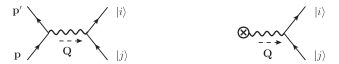
Figure 1: Left: The impinging electron collides with another electron in the target material, and excites the latter from state $\ket{j}$ to state $\ket{i}$. Right: An equivalent description where the effect of incident electron is represented with a source term. See text for details.

The EELS provides the spectrum information of the energy transferred from a fast impinging electron to the target material, which is deposited either in the form of electron-hole pairs, or collective excitations (plasmons). We begin the discussion with the diagram in the left panel in Fig. 1 that describes the process where one incident electron excites another in the target material from state $\ket{j}$ to state $\ket{i}$. With the Feynman rules summarized in appendix of Ref. (Liang:2020ryg, ), relevant amplitude reads as

$$i\mathcal{M} = -iV_{\mathrm{Cou}}\left(\mathbf{Q}\right)\braket{i}{e^{i\mathbf{Q}\cdot\hat{\mathbf{x}}}}{j}$$ (1)

$$= -i\frac{4\pi\alpha}{Q^{2}}\braket{i}{e^{i\mathbf{Q}\cdot\hat{\mathbf{x}}}}{j},$$

where $\mathbf{Q}=\mathbf{p}-\mathbf{p}^{\prime}$, with $\mathbf{p}$ ($\mathbf{p}^{\prime}$) is the electron momentum before (after) the scattering, $V_{\mathrm{Cou}}$ represents the propagator of the electron-electron Coulomb interaction, and $\alpha$ is the electromagnetic fine structure constant. To calculate the cross section, one needs to average over the initial states and sum over the final states of electrons in crystal, at a finite temperature $T$, so it is more convenient to treat this problem in the context of the linear response theory. To this end, the effects brought by the incident electron is regarded as a perturbation exerted onto the electronic system of the target material, which can be summarized as the following effective Hamiltonian for the electrons in solids (i.e., the source term illustrated in the right panel in Fig. 1):

$$\hat{H}_{I}\left(t\right)=\hat{H}_{I}e^{i\omega_{p^{\prime}p}t}$$

$$=V_{\mathrm{Cou}}\left(\mathbf{Q}\right)\int e^{i\mathrm{\mathbf{Q}\cdot\mathbf{x}}}\,\hat{\rho}_{I}\left(\mathbf{x},t\right)\mathrm{d}^{3}x\,e^{i\omega_{p^{\prime}p}t}$$

$$=V_{\mathrm{Cou}}\left(\mathbf{Q}\right)\int e^{i\mathrm{\mathbf{Q}\cdot\mathbf{x}}}\,\hat{\psi}_{I}^{\dagger}\left(\mathbf{x},t\right)\hat{\psi}_{I}\left(\mathbf{x},t\right)\mathrm{d}^{3}x\,e^{i\omega_{p^{\prime}p}t},$$ (2)

where $\hat{\rho}_{I}$ and $\hat{\psi}_{I}$ are the density and the field operators of the electron, respectively, and $\omega_{p^{\prime}p}=p^{\prime 2}/2m_{e}-p^{2}/2m_{e}$ is the energy difference between the outgoing and incoming electron ($m_{e}$ is the electron mass). Thus the averaging and summing procedure can be expressed as a correlation function

$$S_{\hat{H}_{I}^{\dagger}\hat{H}_{I}}\left(-\omega_{p^{\prime}p}\right) = \sum_{i,\,j}p_{j}\left|\braket{i}{\hat{H}_{I}}{j}\right|^{2}\left(2\pi\right)\delta\left(\varepsilon_{i}-\varepsilon_{j}+\omega_{p^{\prime}p}\right)$$ (3)

$$= \int_{-\infty}^{+\infty}\left\langle\hat{H}_{I}^{\dagger}\left(0\right)\hat{H}_{I}\left(t\right)\right\rangle e^{i\omega_{p^{\prime}p}t}\mathrm{d}t,$$

where $p_{j}$ is the thermal distribution of the initial state $\ket{j}$, and the symbol $\left\langle\cdots\right\rangle$ represents the thermal average. At this stage, one can insert this correlation function into the formula for the cross section (Fermi’s golden rule) in terms of the inverse dielectric function $\epsilon^{-1}\left(\mathbf{Q},\omega\right)$,

$$\sigma = \int\frac{\mathrm{d}^{3}Q\,\mathrm{d}^{3}p^{\prime}}{\left(2\pi\right)^{3}}\frac{S_{\hat{H}_{I}^{\dagger}\hat{H}_{I}}\left(\omega\right)\delta^{3}\left(\mathbf{p}^{\prime}-\mathbf{p}+\mathbf{Q}\right)\delta\left(\omega_{p^{\prime}p}+\omega\right)}{v}\mathrm{d}\omega$$ (4)

$$\simeq V\int\frac{\mathrm{d}^{3}Q}{\left(2\pi\right)^{3}}\frac{2V_{\mathrm{Cou}}\left(\mathbf{Q}\right)}{v}\mathrm{Im}\left[\frac{-1}{\epsilon\left(\mathbf{\mathbf{Q}},\omega\right)}\right]$$

$$\times\delta\left(\frac{\left|\mathbf{Q}\right|^{2}}{2m_{e}}-\mathbf{v}\cdot\mathbf{Q}+\omega\right)\mathrm{d}\omega,$$

where $v$ is the velocity of the incident electron, and $V$ represents the volume of the material. In above derivation we utilize the fluctuation-dissipation theorem

$$S_{\hat{H}_{I}^{\dagger}\hat{H}_{I}}\left(\omega\right)=i\frac{\left[\chi_{\hat{H}_{I}^{\dagger}\hat{H}_{I}}\left(\omega+i0^{+}\right)-\chi_{\hat{H}_{I}^{\dagger}\hat{H}_{I}}\left(\omega-i0^{+}\right)\right]}{1-e^{-\beta\omega}}$$

$$\simeq iV\left|V_{\mathrm{Cou}}\left(\mathbf{Q}\right)\right|^{2}\,\left[\chi_{\hat{\rho}\hat{\rho}}\left(\mathbf{Q},\,\omega+i0^{+}\right)-\chi_{\hat{\rho}\hat{\rho}}\left(\mathbf{Q},\,\omega-i0^{+}\right)\right]$$

$$=-2V\left|V_{\mathrm{Cou}}\left(\mathbf{Q}\right)\right|^{2}\,\mathrm{Im}\left[\chi_{\hat{\rho}\hat{\rho}}^{\mathrm{r}}\left(\mathbf{\mathbf{Q}},\,\omega\right)\right]$$

$$=2V\,V_{\mathrm{Cou}}\left(\mathbf{Q}\right)\,\mathrm{Im}\left[\frac{-1}{\epsilon\left(\mathbf{\mathbf{Q}},\omega\right)}\right],$$ (5)

where $\beta=1/T$ is the inverse temperature, and we adopt the zero-temperature approximation $1-e^{-\beta\omega}\approx 1$; $\chi_{\hat{A}\hat{B}}\left(z\right)$ is the master function of the correlation functions of the operators $\hat{A}$ and $\hat{B}$, which yields relevant retarded correlation function $\chi_{\hat{A}\hat{B}}^{\mathrm{r}}\left(\omega\right)=\chi_{\hat{A}\hat{B}}\left(\omega+i0^{+}\right)$ and advanced correlation function $\chi_{\hat{A}\hat{B}}^{\mathrm{a}}\left(\omega\right)=\chi_{\hat{A}\hat{B}}\left(\omega-i0^{+}\right)$ in momentum space; the inverse dielectric function in the last line connects the retarded density-density correlation function $\chi_{\hat{\rho}\hat{\rho}}^{\mathrm{r}}\left(\mathbf{\mathbf{Q}},\,\omega\right)$ through the following relation,

$$\frac{1}{\epsilon\left(\mathbf{Q},\omega\right)} = 1+V_{\mathrm{Cou}}\left(\mathbf{Q}\right)\chi_{\hat{\rho}\hat{\rho}}^{\mathrm{r}}\left(\mathbf{Q},\,\omega\right).$$ (6)

On the other hand, the Schwinger-Dyson equation for the screen Coulomb interaction connects the dielectric function and the the polarizability $\Pi\left(\mathbf{Q},\,\omega\right)$ through the relation

$$\epsilon\left(\mathbf{Q},\,\omega\right) = 1-V_{\mathrm{Cou}}\left(\mathbf{Q}\right)\Pi\left(\mathbf{Q},\,\omega\right).$$ (7)

In the random phase approximation (RPA), $\Pi\left(\mathbf{Q},\,\omega\right)$ is approximated by the electron-hole loop and thus the dielectric function can be expressed as

$$\epsilon\left(\mathbf{\mathbf{Q}},\omega\right) \simeq 1-\frac{V_{\mathrm{Cou}}\left(\mathbf{Q}\right)}{V}\sum_{i,j}\frac{\left|\braket{i}{e^{i\mathbf{\mathbf{Q}}\cdot\hat{\mathbf{x}}}}{j}\right|^{2}}{\varepsilon_{i}-\varepsilon_{j}-\omega-i0^{+}}\left(n_{i}-n_{j}\right),$$

where $n_{i}$ ($n_{j}$) and $\varepsilon_{i}$ ($\varepsilon_{j}$) denote the occupation number and the energy of the state $\ket{i}$ ($\ket{j}$), respectively. Plugging the dielectric function Eq. (LABEL:eq:RPA-dielectric-fucnition0) into Eq. (4) yields the EELS cross section for the HEG.

II.2 EELS in crystalline solids

Above discussion of the EELS for the HEG can be straightforwardly extended to the case in crystal structure, as long as one takes into consideration the LFEs in the crystalline environment. In crystalline solid where the translational symmetry for continuous space reduces to that for the crystal lattice, the correlation functions can no longer be expressed as differences of the space-time coordinates. In this case, any function periodic in position $\chi\left(\mathbf{x},\mathbf{x}^{\prime};\omega\right)$ can be expressed in the reciprocal space as the following,

$$\chi\left(\mathbf{x},\mathbf{x}^{\prime};\omega\right) = \frac{1}{V}\sum_{\mathbf{k}\in 1\mathrm{BZ}}\sum_{\mathbf{G},\mathbf{G}^{\prime}}e^{i\left(\mathbf{k}+\mathbf{G}\right)\cdot\mathbf{x}}$$ (9)

$$\times\chi_{\mathbf{G},\mathbf{G}^{\prime}}\left(\mathbf{k},\omega\right)e^{-i\left(\mathbf{k}+\mathbf{G}^{\prime}\right)\cdot\mathbf{x}^{\prime}}$$

where $\chi_{\mathbf{G},\mathbf{G}^{\prime}}\left(\mathbf{k};\omega\right)$ is the reciprocal matrix with $\mathbf{G}$ and $\mathbf{G}^{\prime}$ being reciprocal lattice vectors and $\mathbf{k}$ is restricted to the 1BZ, which can be determined with the Fourier transformation

$$\chi_{\mathbf{G},\mathbf{G}^{\prime}}\left(\mathbf{k},\omega\right) = \frac{1}{V}\int\mathrm{d}^{3}x\,\mathrm{d}^{3}x\,^{\prime}e^{-i\left(\mathbf{k}+\mathbf{G}\right)\cdot\mathbf{x}}$$ (10)

$$\times\chi\left(\mathbf{x},\mathbf{x}^{\prime};\omega\right)\,e^{i\left(\mathbf{k}+\mathbf{G}^{\prime}\right)\cdot\mathbf{x}^{\prime}}.$$

As a consequence, for an arbitrary momentum transfer $\mathbf{Q}$, which can be split into a reduced momentum confined in the 1BZ, and a reciprocal one, i.e., $\mathbf{\mathbf{Q}}=\mathbf{q}+\mathbf{G}$, one obtains the following correspondence in crystalline environment:

$$\chi_{\hat{\rho}\hat{\rho}}^{\mathrm{r}}\left(\mathbf{Q},\,\omega\right) \rightarrow \chi_{\hat{\rho}\hat{\rho}\,\mathbf{G},\mathbf{G}}^{\mathrm{r}}\left(\mathbf{q},\omega\right)$$ (11)

$$= \frac{1}{V}\int\mathrm{d}^{3}x\,\mathrm{d}^{3}x\,^{\prime}e^{-i\left(\mathbf{q}+\mathbf{G}\right)\cdot\mathbf{x}}$$

$$\times\chi_{\hat{\rho}\hat{\rho}}^{\mathrm{r}}\left(\mathbf{x},\mathbf{x}^{\prime};\omega\right)\,e^{i\left(\mathbf{q}+\mathbf{G}\right)\cdot\mathbf{x}^{\prime}}.$$

$\chi_{\hat{\rho}\hat{\rho}\,\mathbf{G},\mathbf{G}^{\prime}}^{\mathrm{r}}$ is connected to the inverse microscopic dielectric matrix $\epsilon_{\mathbf{G},\mathbf{G}^{\prime}}$ through the relation

$$\epsilon_{\mathbf{G},\mathbf{G}^{\prime}}^{-1}\left(\mathbf{q},\omega\right) = \delta_{\mathbf{G},\mathbf{G}^{\prime}}+V_{\mathbf{G},\mathbf{G}^{\prime}}^{\mathrm{Cou}}\left(\mathbf{q}\right)\chi_{\hat{\rho}\hat{\rho}\,\mathbf{G},\mathbf{G}^{\prime}}^{\mathrm{r}}\left(\mathbf{q},\,\omega\right),$$ (12)

where $V_{\mathbf{G},\mathbf{G}^{\prime}}^{\mathrm{Cou}}\left(\mathbf{q}\right)$=$V_{\mathrm{Cou}}\left(\mathbf{q}+\mathbf{G}\right)\delta_{\mathbf{G},\mathbf{G}^{\prime}}$=$4\pi\alpha\delta_{\mathbf{G},\mathbf{G}^{\prime}}/\left|\mathbf{q}+\mathbf{G}\right|^{2}$ is obtained from Eq. (10). Consequently, the expression for the cross section for the HEG in Eq. (4) can be extended to the case in crystal structure as follows,

$$\sigma \simeq V\sum_{\mathbf{G}}\int_{1\mathrm{BZ}}\frac{\mathrm{d}^{3}q}{\left(2\pi\right)^{3}}\frac{2\,V_{\mathrm{Cou}}\left(\mathbf{G}+\mathbf{q}\right)}{v}\,\mathrm{Im}\left[\epsilon_{\mathbf{G},\mathbf{G}}^{-1}\left(\mathbf{q},\omega\right)\right]\,\delta\left[\frac{\left|\mathbf{G}+\mathbf{q}\right|^{2}}{2m_{e}}-\mathbf{v}\cdot\mathbf{\left(\mathbf{G}+\mathbf{q}\right)}+\omega\right]\mathrm{d}\omega$$ (13)

$$= \sum_{\mathbf{G}}\sum_{\mathbf{\mathbf{q}\in 1\mathrm{BZ}}}\int\frac{2\,V_{\mathrm{Cou}}\left(\mathbf{G}+\mathbf{q}\right)}{v}\,\mathrm{Im}\left[\epsilon_{\mathbf{G},\mathbf{G}}^{-1}\left(\mathbf{q},\omega\right)\right]\,\delta\left[\frac{\left|\mathbf{G}+\mathbf{q}\right|^{2}}{2m_{e}}-\mathbf{v}\cdot\mathbf{\left(\mathbf{G}+\mathbf{q}\right)}+\omega\right]\mathrm{d}\omega.$$

In this study, we adopt the RPA for the microscopic dielectric matrix:

$$\epsilon_{\mathbf{G},\mathbf{G}^{\prime}}\left(\mathbf{q},\omega\right) = \delta_{\mathbf{G},\mathbf{G}^{\prime}}-\frac{V_{\mathbf{G},\mathbf{G}}^{\mathrm{Cou}}\left(\mathbf{q}\right)}{V}\sum_{i,j}\frac{\braket{i}{e^{i\left(\mathbf{\mathbf{\mathbf{q}+\mathbf{G}}}^{\prime}\right)\cdot\hat{\mathbf{x}}}}{j}\braket{j}{e^{-i\left(\mathbf{\mathbf{\mathbf{q}+\mathbf{G}}}\right)\cdot\hat{\mathbf{x}}}}{i}}{\varepsilon_{ij}-\omega-i0^{+}}\left(n_{i}-n_{j}\right).$$ (14)

In practice, the inverse dielectric function $\epsilon_{\mathbf{G},\mathbf{G}}^{-1}\left(\mathbf{q},\omega\right)$ is obtained via directly inverting the dielectric matrix in Eq. (14).

II.3 Electron excitation induced by DM particles

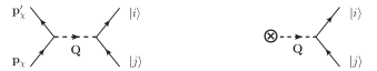
Figure 2: Left: Feynman diagram for the impinging DM particle collides with an electron in the target material, and excites it from state $\ket{j}$ to state $\ket{i}$. Right: An equivalent description where the effect of incident DM particle is replaced with a source term.

Above discussion of the EELS can be transplanted in a parallel manner to the scenario where the impinging particle is a DM particle (see Fig. 2). In this case, the Coulomb potential $V_{\mathrm{Cou}}\left(\mathbf{Q}\right)$ should be replaced by the DM-electron interaction $V_{\chi e}\left(\mathbf{Q}\right)$ leading to Eq. (5), which yields

$$S_{\hat{H}_{I}^{\dagger}\hat{H}_{I}}\left(\omega\right) = 2V\,\frac{\left|V_{\chi e}\left(\mathbf{Q}\right)\right|^{2}}{V_{\mathrm{Cou}}\left(\mathbf{\mathbf{Q}}\right)}\mathrm{Im}\left[\frac{-1}{\epsilon\left(\mathbf{Q},\omega\right)}\right]$$ (15)

for the case of HEG. $V_{\chi e}\left(\mathbf{Q}\right)$ is connected to the relativistic scattering amplitude $\mathcal{M}_{\mathrm{R}}\left(\mathbf{Q}\right)$ in the low-energy limit through the relation

$$V_{\chi e}\left(\mathbf{Q}\right) = \frac{\mathcal{M}_{\mathrm{R}}\left(\mathbf{Q}\right)}{4\,m_{\chi}m_{e}},$$ (16)

with $m_{\chi}$ being the DM mass.

It should be noted that, above formalism in terms of the dielectric function (i.e., density-density correlation function, see Eq. (2)) applies only for a limited set of Lorentz invariant DM interactions (Trickle:2020oki, ; Mitridate:2021ctr, ). Because other momentum- or/and angular momentum-dependent effective operator, as a byproduct of matching onto a non-relativistic effective field theory from the initial Lorentz invariant interaction, will also emerge and couple to even more complicated forms of correlation functions (e.g., current-current correlation) beyond the density-density correlation. To be concrete, we consider two simple examples (Knapen:2021run, ; Hochberg:2021pkt, ) that apply for above discussion: $\mathcal{L}\supset g_{\chi}\phi\bar{\chi}\chi+g_{e}\phi\bar{e}e$, where a Dirac DM fermion couples to an electron through a scale $\phi$, and in an analogous fashion, through a vector $V_{\mu}$, i.e., with Lagrangian $\mathcal{L}\supset g_{\chi}V_{\mu}\bar{\chi}\gamma^{\mu}\chi+g_{e}V_{\mu}\bar{e}\gamma^{\mu}e$. In these cases, the DM component only couples to the electric density at the leading order, as the form shown in Eq. (2).

Therefore, the DM excitation cross section parallel to Eq. (13) can be expressed as

$$\sigma = \sum_{\mathbf{G}}\sum_{\mathbf{\mathbf{q}\in 1\mathrm{BZ}}}\int\frac{2\,\left|V_{\chi e}\left(\mathbf{\mathbf{G}+\mathbf{q}}\right)\right|^{2}}{v\,V_{\mathrm{Cou}}\left(\mathbf{G}+\mathbf{q}\right)}\,\mathrm{Im}\left[-\epsilon_{\mathbf{G},\mathbf{G}}^{-1}\left(\mathbf{q},\omega\right)\right]$$ (17)

$$\times\delta\left[\frac{\left|\mathbf{G}+\mathbf{q}\right|^{2}}{2m_{\chi}}-\mathbf{v}\cdot\mathbf{\left(\mathbf{G}+\mathbf{q}\right)}+\omega\right]\mathrm{d}\omega.$$

For the simplest contact interaction, $V_{\chi e}\left(\mathbf{Q}\right)$ can be replaced by the DM-electron cross section $\sigma_{\chi e}$ as the following,

$$\left|V_{\chi e}\left(\mathbf{Q}\right)\right|^{2} = \frac{\pi\,\sigma_{\chi e}}{\mu_{\chi e}^{2}},$$ (18)

with $\mu_{\chi e}=m_{e}\,m_{\chi}/\left(m_{e}+m_{\chi}\right)$ being the reduced mass of the DM-electron pair. Consequently, one obtains the excitation rate of the electrons in crystalline solid induced by DM particle as the following:

$$R = \frac{\rho_{\chi}}{m_{\chi}}\left\langle\sigma v\right\rangle$$

$$= \frac{\rho_{\chi}}{m_{\chi}}\frac{\sigma_{\chi e}}{4\,\alpha\,\mu_{\chi e}^{2}}\int\mathrm{d}\omega\int\mathrm{d^{3}}v\,\frac{f_{\chi}\left(\mathbf{v}\right)}{v}\sum_{\mathbf{G}}\sum_{\mathbf{\mathbf{q}\in 1\mathrm{BZ}}}\,\left|\mathbf{G}+\mathbf{q}\right|$$

$$\times\mathrm{Im}\left[-\epsilon_{\mathbf{G},\mathbf{G}}^{-1}\left(\mathbf{q},\omega\right)\right]\Theta\left[v-v_{\mathrm{min}}\left(\left|\mathbf{G}+\mathbf{q}\right|,\,\omega\right)\right],$$

where the bracket $\left\langle\cdots\right\rangle$ denotes the average over the DM velocity distribution, $\rho_{\chi}=0.3\,\mathrm{GeV/cm^{3}}$ represents the DM local density, and $\Theta$ is the Heaviside step function, with

$$v_{\mathrm{min}}\left(\left|\mathbf{G}+\mathbf{q}\right|,\,\omega\right) = \frac{\left|\mathbf{G}+\mathbf{q}\right|}{2\,m_{\chi}}+\frac{\omega}{\left|\mathbf{G}+\mathbf{q}\right|}.$$ (20)

The DM velocity distribution is approximated as a truncated Maxwellian form in the Galactic rest frame, i.e., $f_{\chi}\left(\mathbf{v}\right)\propto\exp\left[-\left|\mathbf{v}+\mathbf{v}_{\mathrm{e}}\right|^{2}/v_{0}^{2}\right]$$\Theta\left(v_{\mathrm{esc}}-\left|\mathbf{v}+\mathbf{v}_{\mathrm{e}}\right|\right)$, with the Earth’s (or approximately, the Sun’s) velocity $v_{\mathrm{e}}=230\,\mathrm{km/s}$, the dispersion velocity $v_{0}=220\,\mathrm{km/s}$ and the Galactic escape velocity $v_{\mathrm{esc}}=544\,\mathrm{km/s}$. If one ignores the orientation of the crystal structure with respect to the Galaxy and integrate out the angular parts of the velocity $\mathbf{v}$ and momentum transfer $\left|\mathbf{G}+\mathbf{q}\right|$, the velocity distribution is considered as isotropic.

Besides, if one assumes the electromagnetic interaction is weak enough so as to take only the terms up to first order in the resolvent $\left(I-M\right)^{-1}=I+M+M^{2}+\cdots$, where the identity matrix $I$ and $M$ represent the first and the the second terms in Eq. (14), respectively, the inverse matrix in Eq. (LABEL:eq:eventRate) can be approximated as (see Eq. (14))

$$\mathrm{Im}\left[-\epsilon_{\mathbf{G},\mathbf{G}}^{-1}\left(\mathbf{q},\omega\right)\right]\simeq\mathrm{Im}\left[\epsilon_{\mathbf{G},\mathbf{G}}\left(\mathbf{q},\omega\right)\right]$$

$$=2\times\frac{4\pi^{2}\alpha}{V\,\left|\mathbf{q}+\mathbf{G}\right|^{2}}\,\sum_{i^{\prime}}^{c}\sum_{i}^{v}\,\sum_{\mathbf{k}^{\prime},\mathbf{\mathbf{k}\in 1\mathrm{BZ}}}\left|\braket{i^{\prime}\mathbf{k}^{\prime}}{e^{i\left(\mathbf{\mathbf{\mathbf{q}+\mathbf{G}}}\right)\cdot\hat{\mathbf{x}}}}{i\mathbf{k}}\right|^{2}\,\delta\left(\varepsilon_{i^{\prime}\mathbf{k}^{\prime}}-\varepsilon_{i\mathbf{k}}-\omega\right),$$ (21)

where the Bloch electronic states $\left\{\ket{i\mathbf{k}}\right\}$ are explicitly labeled with discrete band indices $\left\{i\right\}$ and crystal momenta $\left\{\mathbf{k}\right\}$ confined to the 1BZ. Thus above event rate Eq. (LABEL:eq:eventRate) is explicitly written as

$$R = \frac{\rho_{\chi}}{m_{\chi}}\frac{\sigma_{\chi e}}{4\,\alpha\,\mu_{\chi e}^{2}}\int\mathrm{d}\omega\int\mathrm{d^{3}}v\,\frac{f_{\chi}\left(\mathbf{v}\right)}{v}\sum_{\mathbf{G}}\sum_{\mathbf{\mathbf{q}\in 1\mathrm{BZ}}}\,\left|\mathbf{G}+\mathbf{q}\right|\,\mathrm{Im}\left[-\epsilon_{\mathbf{G},\mathbf{G}}^{-1}\left(\mathbf{q},\omega\right)\right]\,\Theta\left[v-v_{\mathrm{min}}\left(\left|\mathbf{G}+\mathbf{q}\right|,\,\omega\right)\right]$$ (22)

$$\simeq \frac{\rho_{\chi}}{m_{\chi}}\frac{2\pi^{2}\sigma_{\chi e}}{\mu_{\chi e}^{2}}\,V\int\mathrm{d^{3}}v\,\frac{f_{\chi}\left(\mathbf{v}\right)}{v}\sum_{\mathbf{G}}\sum_{i^{\prime}}^{c}\sum_{i}^{v}\int_{1\mathrm{BZ}}\frac{\mathrm{d}^{3}k^{\prime}}{\left(2\pi\right)^{3}}\int_{1\mathrm{BZ}}\frac{\mathrm{d}^{3}k}{\left(2\pi\right)^{3}}\frac{\left|\int_{\Omega}\mathrm{d}^{3}x\,u_{i^{\prime}\mathbf{k}^{\prime}}^{*}\left(\mathbf{x}\right)\,e^{i\mathbf{\mathbf{G}}\cdot\mathbf{x}}\,u_{i\mathbf{k}}\left(\mathbf{x}\right)\right|^{2}}{\left|\mathbf{k}^{\prime}-\mathbf{k}+\mathbf{G}\right|}$$

$$\times\Theta\left[v-v_{\mathrm{min}}\left(\left|\mathbf{k}^{\prime}-\mathbf{k}+\mathbf{G}\right|,\,\varepsilon_{i^{\prime}\,\mathbf{k}^{\prime}}-\varepsilon_{i\,\mathbf{k}}\right)\right],$$

where the periodic wave functions $\left\{u_{i\mathbf{k}}\left(\mathbf{x}\right)\right\}$ are normalized within the unit cell, over which the integral $\int_{\Omega}\mathrm{d}^{3}x\,\left(\cdots\right)$ is performed. It is straightforward to verify that the event rate in Eq. (22) exactly corresponds to the case without the screening effect (Essig:2015cda, ).

II.4 Screening effect in DM direct detection

Now we put above formulas into practical computations. We will concretely calculate the screening effect on sensitivities of diamond- and silicon-base detectors to the Galactic DM halo, discussing the local field effects in different computational approaches, and compare our results with those calculated with the $\mathtt{GPAW}$ code (Knapen:2021run, ).

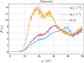
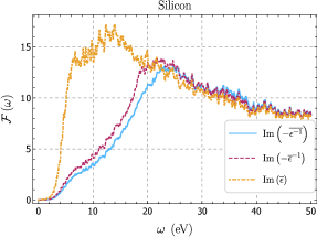
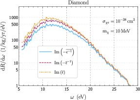
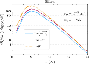
Figure 3: Top: The nondimensional factor $\mathcal{F}\left(\omega\right)$ defined in Eq. (26) for the inverse dielectric functions $\mathrm{Im}\left[-\overline{\epsilon^{-1}}\right]$ (blue solid), $\mathrm{Im}\left[-\overline{\epsilon}^{-1}\right]$ (red dashed) and $\mathrm{Im}\left[\overline{\epsilon}\right]$ (orange dot-dashed) for diamond (left) and silicon (right), respectively. Bottom: The screening effect on differential rate spectra in diamond (left) and silicon targets (right), for a $10\,\mathrm{MeV}$ DM particle and cross section $\sigma_{\chi e}=10^{-38}\,\mathrm{cm}^{2}$, respectively. See text for details.

In practical computation, it is convenient to reinterpret the integration over the momenta $\mathbf{G}$ and $\mathbf{q}$ in Eq. (LABEL:eq:eventRate) in terms of variable $\left|\mathbf{q}+\mathbf{G}\right|$. To this end, we first calculate the angular-averaged inverse dielectric function (Knapen:2021run, ):

$$\overline{\epsilon^{-1}}\left(Q,\omega\right) \equiv \frac{1}{N\left(Q\right)}\sum_{\mathbf{q},\mathbf{G}}\epsilon_{\mathbf{G},\mathbf{G}}^{-1}\left(\mathbf{q},\omega\right)\delta_{Q,\,\left|\mathbf{q}+\mathbf{G}\right|},$$ (23)

where $N\left(Q\right)\equiv\sum_{\mathbf{q},\mathbf{G}}\delta_{Q,\,\left|\mathbf{q}+\mathbf{G}\right|}$, and $Q$ is an arbitrary transferred momentum beyond the 1BZ. Note that this definition takes into account the LFEs. As a consequence, the excitation rate in Eq. (LABEL:eq:eventRate) can be equivalently recast as

$$R=\frac{\rho_{\chi}}{m_{\chi}}\frac{\sigma_{\chi e}\,N_{\mathrm{cell}}}{4\,\alpha\,\mu_{\chi e}^{2}}\int\mathrm{d}\omega\int\mathrm{d^{3}}v\,\frac{f_{\chi}\left(\mathbf{v}\right)}{v}\int\frac{\Omega\,\mathrm{d}^{3}Q}{\left(2\pi\right)^{3}}$$

$$\times Q\,\mathrm{Im}\left[-\overline{\epsilon^{-1}}\left(Q,\omega\right)\right]\,\Theta\left[v-v_{\mathrm{min}}\left(Q,\,\omega\right)\right],$$ (24)

where $N_{\mathrm{cell}}$ is the number of the unit cells in the target material. In addition, there is an alternative definition of the ELF (Knapen:2021run, ), where the inverse dielectric function is obtained by first calculating the directionally averaged dielectric function

$$\overline{\epsilon}\left(Q,\omega\right) \equiv \frac{1}{N\left(Q\right)}\sum_{\mathbf{q},\mathbf{G}}\epsilon_{\mathbf{G},\mathbf{G}}\left(\mathbf{q},\omega\right)\delta_{Q,\,\left|\mathbf{q}+\mathbf{G}\right|},$$ (25)

and then approximating the the inverse dielectric function as $\mathrm{Im}\left[-\overline{\epsilon^{-1}}\left(Q,\omega\right)\right]\simeq\mathrm{Im}\left[-\overline{\epsilon}^{-1}\left(Q,\omega\right)\right]$. This approximation neglects the LFEs because only the information of the diagonal terms of matrix $\epsilon_{\mathbf{G},\mathbf{G}}\left(\mathbf{q},\omega\right)$ is retained in ELF. In a similar manner, the inverse dielectric function for the non-screening case in Eq. (21) can be approximated as $\mathrm{Im}\left[-\overline{\epsilon^{-1}}\left(Q,\omega\right)\right]\simeq\mathrm{Im}\left[\overline{\epsilon}\left(Q,\omega\right)\right]$. So one of our purpose is to investigate the in-medium screening effect of the DM-electron excitation process. Besides, it is interesting to compare the results drawn form the two definitions of the inverse dielectric functions. While the definition Eq. (23) faithfully reproduces the definition in Eq. (LABEL:eq:eventRate), the LFEs are neglected in Eq. (25). To explore the consequence of the LFEs, we concretely compute the excitation rates for diamond and silicon targets based on Eq. (23), and make a comparison with the results obtained from the definition Eq. (25).

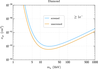
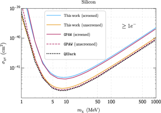
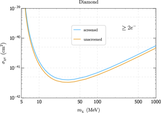
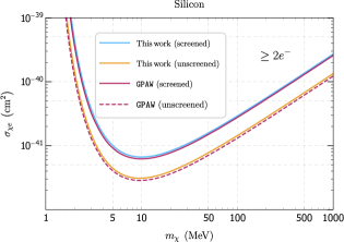
Figure 4: 95% C.L. constraints on the DM-electron cross section $\sigma_{\chi e}$ with (blue) and without (orange) the screening effect for the diamond target, assuming $1e^{-}$ (upper left) and $2e^{-}$(bottom left) thresholds. Upper right: Sensitivities of various calculations for silicon target at the 95% C.L.: with (blue) and without (orange) screening effect in this work, $\mathtt{GPAW}$ estimation (Knapen:2021run, ) for screened (red solid) and unscreened cases (red dashed), and $\mathtt{QEDark}$ (Essig:2015cda, ) (black dotted), respectively. All constraints are calculated with negligible background and a 1kg-year exposure. For comparison purpose, the DM distribution parameters $\rho_{\chi}=0.4\,\mathrm{GeV/cm^{3}}$, $v_{\mathrm{e}}=240\,\mathrm{km/s}$, $v_{0}=230\,\mathrm{km/s}$ and $v_{\mathrm{esc}}=600\,\,\mathrm{km/s}$ are adopted in alignment. Bottom right: 95% C.L $2e^{-}$ threshold sensitivities for silicon target: with (blue) and without (orange) screening effect in this work, $\mathtt{GPAW}$ estimations (Knapen:2021run, ) for screened (red solid) and unscreened cases (red dashed), respectively. See text for details.

Using $\mathtt{Quantum\>Espresso}$ package (Giannozzi_2009, ) plus a norm-conserving pseudopotential (PhysRevLett.43.1494, ), we perform the DFT calculation to obtain the Bloch eigenfunctions and eigenvalues using the local-density approximation (PhysRevB.23.5048, ) for the exchange-correlation functional, on a uniform 6$\times$6$\times$6 (5$\times$5$\times$5) $k$-point mesh for diamond (silicon) via the Monkhorst-Pack (PhysRevB.13.5188, ) scheme. A core cutoff radius of $1.3\,\mathrm{Bohr}$ ($1.8\,\mathrm{Bohr}$) is adopted and the outermost four electrons are treated as valence for both diamond and silicon. The energy cut $\varepsilon_{\mathrm{cut}}$ is set to $200\,\mathrm{Ry}$ ($70\,\mathrm{Ry}$) and lattice constant 3.577 Å  (5.429 Å) for diamond (silicon) obtained from experimental data is adopted. The matrix $\epsilon_{\mathbf{G},\mathbf{G}^{\prime}}^{-1}$ is calculated via directly inverting the matrix Eq. (14) at the RPA level with the $\mathtt{YAMBO}$ package (Marini2009.yambo, ), with a matrix cutoff of $50\,\mathrm{Ry}$ ($20\,\mathrm{Ry}$), corresponding to $Q\leq 30\,\mathrm{keV}$ ($20\,\mathrm{keV}$) for diamond (silicon). An energy bin width $\Delta\omega=0.05\,\mathrm{eV}$ is adopted within the range from $0$ to $50\,\mathrm{eV}$.

In order to gauge the screening effect and the difference between the two ELFs, we introduce the following nondimensional factor and present it in the upper row of Fig. 3,

$$\mathcal{F}\left(\omega\right) = \sum_{\mathbf{G}}\int_{1\mathrm{BZ}}\frac{\varOmega\,\mathrm{d}^{3}q}{\left(2\pi\right)^{3}}\,\mathrm{Im}\left[-\epsilon_{\mathbf{G},\mathbf{G}}^{-1}\left(\mathbf{q},\omega\right)\right]$$ (26)

$$= \int\frac{\varOmega\,\mathrm{d}^{3}Q}{\left(2\pi\right)^{3}}\,\mathrm{Im}\left[-\overline{\epsilon^{-1}}\left(Q,\omega\right)\right],$$

for the case of unscreened, screened with LFEs and screened without LFEs, respectively. While it is evident from the top panel of Fig. 3 that the screening effect is remarkable in the low-energy regime ($\omega\lesssim 30\,\mathrm{eV}$ for diamond and $\omega\lesssim 20\,\mathrm{eV}$ for silicon), the factor $\mathcal{F}\left(\omega\right)$ calculated from the dielectric function $\mathrm{Im}\left[-\overline{\epsilon^{-1}}\right]$ in Eq. (23) differs from the one computed from $\mathrm{Im}\left[-\overline{\epsilon}^{-1}\right]$ below Eq. (25) by a factor less than 50% in relevant energy range. In this sense, the dielectric function $\mathrm{Im}\left[-\overline{\epsilon^{-1}}\left(Q,\omega\right)\right]\simeq\mathrm{Im}\left[-\overline{\epsilon}^{-1}\left(Q,\omega\right)\right]$ amounts to an acceptable approximation. In the energy range ($\omega>30\,\mathrm{eV}$ for diamond and $\omega>20\,\mathrm{eV}$ for silicon), the screening effect turns negligible. In the bottom panel of Fig. 3 we present the corresponding differential spectra for diamond (left) and silicon (right) for a DM mass $m_{\chi}=10\,\mathrm{MeV}$ and a benchmark cross section $\sigma_{\chi e}=10^{-38}\,\mathrm{cm}^{2}$, respectively.

To translate the spectrum into excited electron signals, we adopt the model (Essig:2015cda, ) where the secondary electron-hole pairs triggered by the primary one are described with the mean energy per electron-hole pair $\varepsilon$ in high energy recoils. In this picture, the ionization charge $\mathcal{Q}$ is then given by

$$\mathcal{Q}\left(\omega\right) = 1+\left\lfloor\left(\omega-E_{g}\right)/\varepsilon\right\rfloor,$$ (27)

where $\left\lfloor x\right\rfloor$ rounds $x$ down to the nearest integer, and $E_{g}$ denotes the band gap. Thus, from the energy spectra we estimate the sensitivities of a 1 kg-yr diamond (silicon) detector in Fig. 4, adopting a band gap value $E_{g}=5.47\,\mathrm{eV}$ ($1.12\,\mathrm{eV}$) and assuming an average energy $\varepsilon=13\,\mathrm{eV}$ ($3.6\,\mathrm{eV}$) for producing one electron-hole pair for diamond (Kurinsky:2019pgb, ) (silicon (Essig:2015cda, )). In the left panel shown are the 95% C.L. constraints for diamond target with a kg-year exposure for the screened and unscreened cases, assuming $1e^{-}$ (top left) and $2e^{-}$ (bottom left) thresholds. Compared to the $1e^{-}$ threshold, the discrepancy between the screened and unscreened estimations narrows, which can be attributed to the large $\varepsilon=13\,\mathrm{eV}$ that pushes relevant energy into the regime where screening effect begins to wear off. Besides, in order to make comparison with previous $\mathtt{GPAW}$ (Knapen:2021run, ) and $\mathtt{QEDark}$ (Essig:2015cda, ) calculations, we present in the right panel in Fig. 4 the 95% C.L. kg-year exposure projected sensitivities for silicon target with a single electron threshold and no background events. In practical evaluation of dielectric matrix Eq. (14), a small broadening parameter $\eta=0.1\,\mathrm{eV}$ is adopted for both diamond and silicon, instead of an infinitesimal energy width $0^{+}$. A non-vanishing $\eta$ usually brings a long tail extending into the gap region, and hence induces a small contribution to the excitation rate around $E_{g}$. Theoretically, the smaller the parameter $\eta$, the more accurate the computation is, but on the other hand, a smaller $\eta$ also requires a finer energy width $\Delta\omega$ and a denser $k$-point mesh to smear the spectra. As pointed out in Ref. (Knapen:2021bwg, ), there are expected to be $\mathcal{O}\left(1\right)$ uncertainties in the energy range $\omega\lesssim 2E_{g}$, due to the strong fluctuations. While the event rates calculated in this work generally coincide well with the $\mathtt{GPAW}$ results, the latter give a more conservation estimation in the low-energy region for $1e^{-}$ threshold, as a result of different choices of parameter $\eta$. Such uncertainties do not cause a severe problem because they mainly occur in the region plagued by a large noises in most detectors (in the single-electron bin, for instance), and thus are usually excluded from most experimental analyses. If a $2e^{-}$ threshold is adopted, the $\mathtt{YAMBO}$ and $\mathtt{GPAW}$ calculations well coincide in the whole DM mass range, which is clearly seen from the bottom right panel of Fig. 4.

III Light DM particles reflected from the Sun

The idea of detecting the MeV-scale DM particles via solar reflection was first proposed in Ref. (An:2017ojc, ), and is further discussed in Refs. (Chen:2020gcl, ; Emken:2021lgc, ). In this study, our interest is focused on the case where the DM component couples to electron via a heavy mediator, for both scalar ($S\otimes S$) and vector ($V\otimes V$) interaction types, which corresponds to the contact interaction Eq. (18).

Previous investigation (Kopp:2009et, ) pointed out that even for these leptophilic DM models, the effective DM-nucleon cross section arising from lepton-assisted loop-induced processes may compete or even overwhelm that of the DM-electron interaction in DM direct detection experiments. However, a closer analysis shows that, the DM-nucleus cross section in the Sun is so significantly suppressed by a much lighter DM mass (MeV), and a smaller charge number $Z$ (predominantly hydrogen and helium in the Sun) compared to the scenario in direct detection, that it can be safely neglected compared to the DM-electron scattering.

Here we begin with a short review of related physics in the Sun and explain in detail the methodology we adopt in this paper. As in Refs. (An:2017ojc, ; Emken:2021lgc, ), in this work we also take a Monte Carlo simulation approach to describe the solar reflection of the DM particles. Then we generalize discussion in previous sections to the case of solar-reflected DM flux, specifying the screening effect on relevant detection experiments under way, and in plan for the near future.

III.1 Initial condition

The standard description of the DM’s encounter with the Sun has been well established in the literature (Gould:1987ir, ; Gould:1987ww, ; Gould:1991hx, ), which provides an elegant analytic approach in dealing with DM capture and evaporation process. Related arguments can be applied to the present discussion. The starting point of our discussion is the rate $\Gamma$ at which the DM flux reaches the solar surface, which is given by:

$$\Gamma\left(m_{\chi}\right) = \frac{\rho_{\chi}}{m_{\chi}}\pi\int\frac{f_{\chi}\left(\mathbf{u}\right)}{u}\,\mathrm{d}^{3}u\int_{0}^{w^{2}\left(u,R_{\odot}\right)R_{\odot}^{2}}\mathrm{d}J^{2}$$ (28)

$$= \frac{\rho_{\chi}}{m_{\chi}}\pi R_{\odot}^{2}\int\frac{w^{2}\left(u,R_{\odot}\right)}{u}f_{\chi}\left(\mathbf{u}\right)\mathrm{d}^{3}u\int_{0}^{1}\mathrm{d}\left(\sin^{2}\theta\right)$$

$$= \frac{\rho_{\chi}}{m_{\chi}}\pi R_{\odot}^{2}\int\left[\frac{u^{2}+v_{\mathrm{esc}}^{2}\left(R_{\odot}\right)}{u}\right]f_{\chi}\left(\mathbf{u}\right)\mathrm{d}^{3}u,$$

where $R_{\odot}$ is the radius of the Sun, $J$ represents the angular momentum of the DM particle in the solar central field, and $w^{2}\left(u,R_{\odot}\right)=u^{2}+v_{\mathrm{esc}}^{2}\left(R_{\odot}\right)$, with $v_{\mathrm{esc}}\left(r\right)$ being the solar escape velocity at radial distance $r$.

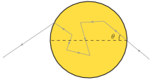
Figure 5: The DM particle enters the body of the sun with an angle $\theta$, collides with solar electrons and finally escapes from the Sun. For the purpose of illustration, the DM trajectory is projected onto a single plane.

Instead of shooting the sampled particles from a large distance with an impact parameter (An:2017ojc, ; Emken:2021lgc, ), we inject them at the surface of the Sun by using the second line in Eq. (28) as the initial condition of the impinging DM flux, which is more convenient if the DM distribution $f_{\chi}\left(\mathbf{u}\right)$ is approximated as isotropic. On one hand, the incident velocity at the surface $w$ is connected to the halo velocity with $\sqrt{u^{2}+v_{\mathrm{esc}}^{2}\left(R_{\odot}\right)}$; on the other, the angle $\theta$ between the incident and the solar radial directions can be determined by angular momentum $J$, i.e., $J^{2}=w^{2}R_{\odot}^{2}\sin^{2}\theta$. So for each particular injection speed $w\left(u,R_{\odot}\right)$ (with weighting factor $\sim w^{2}\left(u,R_{\odot}\right)f_{\chi}\left(u\right)\mathrm{d}u/u$), the directions of the DM particles at surface are sampled evenly in $\sin^{2}\theta$. Fig. 5 shows a schematic sketch of the initial condition for the simulation.

III.2 Propagation in the Sun

Then the trajectories of these sampled DM particles are simulated. To be specific, once a DM particle enters the bulk of the Sun, we first determine whether it will collide with surrounding electrons in the next time step $\Delta t$, which is described with the probability

$$P_{\mathrm{collision}} = 1-\exp\left[-\lambda(t)\,\Delta t\right],$$ (29)

where

$$\lambda\left(t\right) = n_{e}\left(r\right)\left\langle\sigma_{\chi e}\cdot\left|\mathbf{w}-\mathbf{u}_{e}\right|\right\rangle$$ (30)

$$= n_{e}\left(r\right)\,\sigma_{\chi e}\left[\frac{u_{0}}{\sqrt{\pi}}\,\exp\left(-w^{2}/u_{0}^{2}\right)\right.$$

$$\left.+\left(w+\frac{u_{0}^{2}}{2\,w}\right)\mathrm{erf}\left(\frac{w}{u_{0}}\right)\right]$$

is implicitly dependent on temporal parameter $t$, $\left\langle\cdots\right\rangle$ denotes the average over the relative velocity $\mathbf{w}-\mathbf{u}_{e}$ between the DM particle and the surrounding electrons, and $n_{e}\left(r\right)$ is local electron number density. The Maxwellian distribution $f_{e}\left(\mathbf{u}_{e}\right)$ is explicitly written as

$$f_{e}\left(\mathbf{u}_{e}\right) = \left(\sqrt{\pi}u_{0}\right)^{-3}\exp\left(-\frac{u_{e}^{2}}{u_{0}^{2}}\right),$$ (31)

where $u_{0}=$ $\sqrt{2\,T_{\odot}\left(r\right)/m_{e}}$, and $T_{\odot}\left(r\right)$ is the local temperature.

Next, a random number $\xi$ between $0$ and $1$ is generated. If $\xi>P_{\mathrm{collision}}$ we conclude that a scattering event will not happen, and the DM particle propagates to the next location. The gravitational field can be specified by referring to the Standard Sun Model (SSM) AGSS09 (Serenelli:2009yc, ). The number density of the ionized electrons is determined by the condition of charge neutrality (Emken:2021lgc, ). If $\xi<P_{\mathrm{collision}}$, on the other hand, a scattering event is assumed to occur. In this case, further random numbers are generated to pick out the velocity of the electron participating in the collision, as well as the scattering angles in the center-of-mass frame, so that the outgoing state of the scattered DM particle can be determined after a coordinate transformation back to the solar reference (Liang:2018cjn, ).

Then this simulation process continues until one of the following two conditions is satisfied: (1) DM particle reaches the solar surface with a velocity $w>v_{\mathrm{esc}}\left(R_{\odot}\right)$ (if not so, the direction of the velocity is flipped, and the simulation continues until next time the DM particle reaches the surface, and this process is repeated again.); (2) the DM particle is regarded as captured. While the first criterion is straightforward in practice, the second is not so definite, especially considering that a temporarily trapped sub-MeV DM particle is so volatile that after a few collisions it will be kicked out of the solar gravitational well, namely, be evaporated. In this case, the boundary between evaporation and reflection no longer exists, and one should describe them in a unified approach. As will be explained in the following discussions, in practice we specify the criterion for capture such that the DM particle scatters more than 200 times in optically thick regime (i.e., $\sigma_{\chi e}\geq 10^{-36}\,\mathrm{cm}^{2}$ in our practical computation).

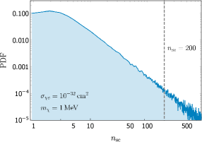
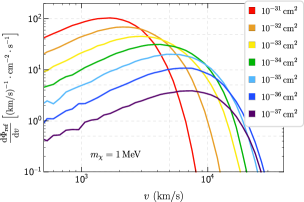
Figure 6: Left: The PDF of scattering number $n_{\mathrm{sc}}$ in simulations, for a DM particle with mass $m_{\chi}=1\,\mathrm{MeV}$ and DM-electron cross section $\sigma_{\chi e}=1\times 10^{-32}\,\mathrm{cm}^{2}.$ Events undergoing more than $200$ collisions are categorized as capture events. Right: The reflected DM differential flux $\mathrm{d}\Phi_{\mathrm{ref}}/\mathrm{d}v$ of a $1\,\mathrm{MeV}$ DM particle with various representative cross sections ranging from $1\times 10^{-37}\,\mathrm{cm}^{2}$ to $1\times 10^{-31}\,\mathrm{cm}^{2}$, respectively. See text for details.

III.3 Spectrum of reflection flux

As DM particle reaches the solar surface, we find out whether it has ever suffered a collision. If not, the sample is categorized as the galactic background and thus is taken out of the tally. If the ongoing DM particle has been scattered more than once and leaves with a velocity $w$ greater than the escape velocity at surface $v_{\mathrm{esc}}\left(R_{\odot}\right)$, this velocity is red-shifted such that $v=\sqrt{w^{2}-v_{\mathrm{esc}}^{2}\left(R_{\odot}\right)+v_{\mathrm{esc}}^{2}\left(D\right)}$ (with $D$ being the Earth-Sun distance), and is put into the prepared bins for the velocity spectrum at the terrestrial detectors. For those leave the Sun with a velocity $w<v_{\mathrm{esc}}\left(R_{\odot}\right)$, we consider them as captured.

When a DM particle dives into the Sun, it may be kicked out after a few collisions, or may be confined to the solar gravitational field for a long time. In the latter case, the DM particle is also regarded as captured. If one assumes that an equilibrium between capture and reflection (which includes evaporation in a more general sense, and annihilation is negligible for a DM with mass $m_{\chi}<1\,\mathrm{GeV}$) is reached today, the instant reflection/evaporation velocity spectrum can be obtained from the spectrum of a large number of simulated reflection/evaporation events that occur over a finite time span.

In practice, it happens frequently that the sampled DM particle is effectively trapped within the Sun in the optically thick parameter regime, and thus a truncation on the simulated number of collisions is necessary. In our practical computation, a cut-off is imposed on the number of scattering $n_{\mathrm{sc}}=200$, which means if a DM particle experiences more than $200$ scatterings it is considered as captured, and the simulation is terminated. These captured DM particles are supposed to be sufficiently thermalized, to evaporate subsequently and hence also contribute to the reflection spectrum.

Since it is unpractical to further simulate the captured DM particles until they are evaporated, we utilize the velocity spectrum of the reflected ones in simulations to deduce that of the captured ones. To be specific, we extrapolate from the statistics of reflection events undergoing $200\geq n_{\mathrm{sc}}>50$ collisions, a number large enough to assume a fully thermalization of an MeV DM particles, to give a trustable description of the evaporation spectrum (of the captured ones), which is then combined with the reflection statistics to give a total spectrum. To get a sense, in the left panel of Fig. 6 we present the probability density function (PDF) of the scattering numbers $n_{\mathrm{sc}}$ for an example DM particle with a mass $m_{\chi}=1\,\mathrm{MeV}$, and a cross section $\sigma_{\chi e}=1\times 10^{-32}\,\mathrm{cm}^{2}$. It is evident that $n_{\mathrm{sc}}=200$ is a sufficiently large cut-off in the sense that the majority of the reflection events can be directly described from simulation. Even for those capture events, the statistics of $n_{\mathrm{sc}}>50$ collisions can provide a reasonable description of their evaporation spectrum.

In the optically thin regime (i.e., $\sigma_{\chi e}<10^{-36}\,\mathrm{cm}^{2}$), however, considering that only a negligible portion of DM particles (in the MeV mass range) are captured after more than a few scatterings, in this case we only consider the reflection events, and neglect the evaporation.

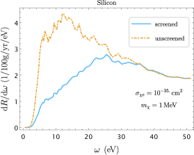
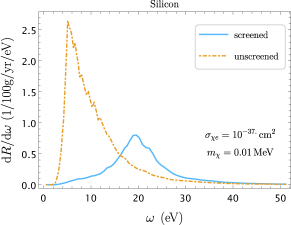
Figure 7: The differential excitation rate in silicon target induced by the solar-reflected DM flux with (blue) and without (orange dashed) the screening effect, respectively, for example DM with $m_{\chi}=1\,\mathrm{MeV}$ and cross section $\sigma_{\chi e}=1\times 10^{-35}\,\mathrm{cm}^{2}$ (left), and with $m_{\chi}=0.01\,\mathrm{MeV}$ and cross section $\sigma_{\chi e}=1\times 10^{-37}\,\mathrm{cm}^{2}$ (right), respectively.

Therefore, the differential flux of the solar reflected DM particle can be expressed with simulation parameters as the following,

$$\frac{\mathrm{d}\Phi_{\mathrm{ref}}}{\mathrm{d}v}\left(v_{i}\right) = \frac{1}{4\pi D^{2}}\left(\frac{N_{i}}{N_{\mathrm{sample}}}\right)\frac{\Gamma\left(m_{\chi}\right)}{\Delta v_{i}},$$ (32)

where $N_{\mathrm{sample}}$ is the total number of the simulated events, $N_{i}$ is event number collected in the $i$-th velocity bin, with $v_{i}$ and $\Delta v_{i}$ being its center value and its width, respectively, and $\Gamma\left(m_{\chi}\right)$ is obtained through calculating the integral in Eq. (28). In order to formulate the experimental event rate from the solar reflection in a parallel fashion to that of the galactic origin, it is necessary to connect the differential reflection flux with the local density of the reflected DM particles as follows,

$$\frac{\mathrm{d}\Phi_{\mathrm{ref}}}{\mathrm{d}v}\left(v\right) =n_{\oplus}vf_{\mathrm{ref}}\left(v\right)$$ , (33)

where $n_{\oplus}$ and $f_{\mathrm{ref}}\left(v\right)$ represent the number density and the velocity distribution of the reflected DM particles at the location of the Earth. Since the the Earth-Sun distance is much larger than the radius of the Sun ($D\sim 200\,R_{\odot}$), the trajectories of the reflected DM particles can be approximated as radially directed. Besides, the anisotropy effect of the halo DM flux (and hence the anisotropy of the reflected DM flux) is neglected in above discussion. In the right panel of Fig. 6 we show the differential flux spectrum of a $1\,\mathrm{MeV}$ DM particle, which, as a whole will appears in the formulation of experimental excitation rate in the following discussions. It is understandable that as the cross section turns smaller, DM particle has a higher chance to reach the hotter core of the Sun, and thus be boosted to a higher speed, as shown in Fig. 6.

III.4 Screening effect in the detection of reflected DM particles

The solar reflected DM particles can be probed with the terrestrial detectors. Such detection strategy is especially preferred for the DM particles in the MeV and sub-MeV mass range, where the DM particles can effectively receive substantial kinetic energy from the hot solar core, and hence are boosted over the conventional detector thresholds. We first formulate the excitation rate of the solar reflection in terms of the ELF, and quantitatively describe the screening effect in relevant process.

By use of Eq. (33), and substituting $\rho_{\chi}/m_{\chi}$ and $\mathrm{d}^{3}v\,f_{\chi}\left(\mathbf{v}\right)$ with $n_{\oplus}$ and $\mathrm{d}vf_{\mathrm{ref}}\left(v\right)$ respectively in Eq. (24), it is straightforward to express the experimental event rate from the solar reflection as follows,

$$R = n_{\oplus}\frac{\sigma_{\chi e}\,N_{\mathrm{cell}}}{4\,\alpha\,\mu_{\chi e}^{2}}\int\mathrm{d}\omega\int\mathrm{d}v\,\frac{f_{\mathrm{ref}}\left(v\right)}{v}\int\frac{\Omega\,\mathrm{d}^{3}Q}{\left(2\pi\right)^{3}}\,$$ (34)

$$\times Q\,\mathrm{Im}\left[-\overline{\epsilon^{-1}}\left(Q,\omega\right)\right]\,\Theta\left[v-v_{\mathrm{min}}\left(Q,\,\omega\right)\right]$$

$$= \frac{\sigma_{\chi e}\,N_{\mathrm{cell}}}{4\,\alpha\,\mu_{\chi e}^{2}}\int\mathrm{d}\omega\int\frac{\mathrm{d}v}{v^{2}}\,\frac{\mathrm{d}\Phi_{\mathrm{ref}}\left(v\right)}{\mathrm{d}v}\int\frac{\Omega\,\mathrm{d}^{3}Q}{\left(2\pi\right)^{3}}\,$$

$$\times Q\,\mathrm{Im}\left[-\overline{\epsilon^{-1}}\left(Q,\omega\right)\right]\,\Theta\left[v-v_{\mathrm{min}}\left(Q,\,\omega\right)\right].$$

Now we can calculate the excitation rates of the solar reflection in terms of the ELF. In the left (right) panel in Fig. 7 shown are the differential rates in silicon target with an exposure $100\,\mathrm{g}\cdot\mathrm{yr}$ for a benchmark DM mass $m_{\chi}=1\,\mathrm{MeV}$ ($0.01\,\mathrm{MeV}$) and a cross section $\sigma_{\chi e}=1\times 10^{-35}\,\mathrm{cm}^{2}$ ($1\times 10^{-37}\,\mathrm{cm}^{2}$), with and without the screening, respectively. In contrast to the case of the halo DM where the event rates are significantly suppressed in energy region $\omega>10\,\mathrm{eV}$ (see Fig. 3), the spectra of the solar reflection extend to a higher energy range beyond $50\,\mathrm{eV}$, a value corresponds to the ionization signal $\mathcal{Q}=14e^{-}$.

Intriguingly, as the velocity of reflected DM increases (i.e., with smaller cross section and smaller mass), the kinetically relevant parameter space begins to overlay the plasmon pole, which features a resonant peak (blue curve) around $20\,\mathrm{eV}$ in the right panel of Fig. 7. While such plasmon resonance can not be directly produced in the scattering of the halo DM particles, its observation has been expected in solar reflection and other possible sources of fast DM particles (Kurinsky:2020dpb, ). It is also noted that unscreened differential rates still dominate in the low energy region, and as a result the in-medium effects may remain suppressing the total event rates when compared to the unscreened calculations.

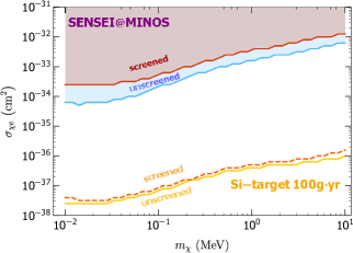
Figure 8: Exclusion curves (90% C.L.) for DM-electron cross section $\sigma_{\chi e}$ from the reflected DM flux. The filled contours illustrate the constraints on $\sigma_{\chi e}$ from the silicon-based SENSEI@MINOS experiment (Barak:2020fql, ) with (red) and without (blue) the screening, respectively. Also shown are the 90% C.L. projected sensitivities of silicon semiconductor with zero background and $100\,\mathrm{g\cdot yr}$ exposure with (orange dashed) and without (orange solid) the screening, respectively.

Then, based on Eq. (34) and the released SENSEI@MINOS results (Barak:2020fql, ), which are presented as 90% C.L. limits on binned ionization signals $\mathcal{Q}=1e^{-},\,2e^{-},\,3e^{-},\,\mathrm{and}\,4e^{-}$, respectively, we calculate the corresponding upper limits of the DM-electron cross section $\sigma_{\chi e}$ in Fig. 8, in both scenarios where the screening effect is neglected and accounted for. Following the analysis in Ref. (Barak:2020fql, ), parameters $E_{g}=1.2\,\mathrm{eV}$, and $\varepsilon=3.8\,\mathrm{eV}$ are adopted in deriving the SENSEI@MINOS constraints. The overall limits are presented as the most stringent one from the four individual signals bins. We also present the projections at 90% C.L. for a future silicon detector with no background and an exposure of $100\,\mathrm{g}\cdot\mathrm{yr}$ in the signal window $\left[2e^{-},\,14e^{-}\right]$, for both the screening and non-screening scenarios. The unscreened constraints are found to be well consistent with those derived in Ref. (Emken:2021lgc, ). It is noted that the screening effect is less remarkable for the reflected DM signals than for the Galactic signals, especially in the optically thin regime, where the signals extend to even higher energies while the screening takes effect in the low energy region.

IV Summary and conclusions

In this paper we perform a detailed derivation of the electronic excitation event rate induced by the DM-electron interaction, taking into account also the screening effect, which is described by the ELF, or the inverse dielectric function. We take the EELS as an example to illustrate how to generalize the discussion of a particle scattering problem at zero temperature to the linear response theory description of the target material exposed to bombardment by DM particles at a finite temperature. In the latter framework the electronic many-body effects are naturally encoded in the dielectric function. We then further extend this procedure to formulate the material response to the DM particles, and perform a DFT calculation for the diamond and silicon targets.

Our numerical calculations not only verify the screening effect for the two targets, but also depict the detailed dependence of screening effect on the energy deposition $\omega$. To summarize, the screening effect is remarkable in the low-energy regime, and as a result, the prediction of excitation rates are suppressed by an $\mathcal{O}\left(1\right)$ factor compared to conventional approach in $\mathtt{QEDark}$ (Essig:2015cda, ). In addition, we also explore the consequence of two different definitions of the angular-averaged inverse dielectric function, namely, the ELFs with and without LFEs. In the first case, one directly averages the inverse of the dielectric matrix to obtain the inverse dielectric function, while in the other case, one first averages the dielectric matrix and then approximate its inverse as the inverse dielectric function. A detailed calculation of diamond and silicon targets shows that the differences between the excitation event rates estimated from these two definitions are well within a factor of $0.5$, providing a direct quantification of the LFEs.

Moreover, we compare the projected sensitivities for silicon calculated using the $\mathtt{YAMBO}$ code with those obtained form the $\mathtt{GPAW}$ estimation (Knapen:2021run, ). While in a broad range of DM mass, the two approaches are found to be well consistent, a noticeable discrepancy appears in the low-mass regime, which originates from the operating parameters adopted in practical implementation. However, such difference disappears if a $2e^{-}$ threshold is adopted in experimental analysis.

In this study we also investigate the in-medium screening effect on detecting the solar-boosted DM flux in silicon-based detectors, which is a promising channel for the probe of MeV and sub-MeV DM particles. With masses in this range, DM particles can be accelerated by the energetic electrons in solar plasma to an energy in the keV scale, so to be detected by conventional semiconductor detectors. Our calculations show that the screening effect brings an $\mathcal{O}\left(0.1\sim 1\right)$ reduction in excitation rates induced by the solar-boosted DM particles, compared to the rates estimated by neglecting the screening. Besides, our calculations verify the production of the plasmon resonance from the scattering between semiconductor targets and fast solar-reflected DM particles, especially in the optically thin regime.

Appendix A An estimate of DM-electron and DM-nucleus cross sections in the Sun

In this Appendix we give a detailed estimate of the DM-electron and loop-induced DM-nucleus cross sections in the Sun, for both scalar ($S\otimes S$) and vector ($V\otimes V$) interaction types discussed in Sec. III. As mentioned in Sec. III, previous study (Kopp:2009et, ) pointed out that even in a wide range of leptophilic DM models there emerges loop-induced DM-hadron interactions, through photons emitted from virtual leptons coupling to the charge of a nucleus.

To summarize the result, first, the typical DM-electron cross section $\sigma\left(\chi e\rightarrow\chi e\right)$ is expressed as $g_{\chi}^{2}g_{e}^{2}\times\sigma_{\chi e}^{0}$, with

$$\sigma_{\chi e}^{0} = \frac{\mu_{\chi e}^{2}}{\pi\Lambda^{4}},$$ (35)

and $\Lambda$ representing the energy scale of the heavy mediators, where perturbative couplings $g_{\chi}$ and $g_{e}$ are also defined. For scalar ($S\otimes S$) type interaction, a DM-nucleus cross section $\sigma\left(\chi N\rightarrow\chi N\right)$ appears at the two-loop level, which is estimated as $\alpha^{2}g_{\chi}^{2}g_{e}^{2}\times\sigma_{\chi N}^{1}$ (see Table I in Ref. (Kopp:2009et, )), where the typical cross section $\sigma_{\chi N}^{1}$ can be written in terms of $\sigma_{\chi e}^{0}$ (eq. (26) in Ref. (Kopp:2009et, ))

$$\sigma_{\chi N}^{1} \approx \left(\frac{\alpha\,Z}{\pi}\right)^{2}\left(\frac{\mu_{\chi N}}{\mu_{\chi e}}\right)^{2}\times\sigma_{\chi e}^{0},$$ (36)

with $\mu_{\chi N}=m_{N}\,m_{\chi}/\left(m_{N}+m_{\chi}\right)$ being the reduced mass of the DM-nucleus pair; for vector ($V\otimes V$) type interaction, the induced DM-nucleus cross section appears at the one-loop level, which is estimated as $g_{\chi}^{2}g_{e}^{2}\times\sigma_{\chi N}^{1}$. It is evident that in the WIMP direct detection, where $\mu_{\chi N}\sim m_{N}\sim m_{\chi}\sim\mathcal{O}\left(10\,\mathrm{GeV}\right)$, thus $\sigma\left(\chi N\rightarrow\chi N\right)\gg\sigma\left(\chi e\rightarrow\chi e\right)$. However, since in the Sun the DM particles predominantly scatter with the hydrogen and helium nuclei ($Z\leq 2$), which brings a suppression factor $\sim 10^{-2}$ compared to $\sigma_{\chi N}^{1}$, and more importantly, a DM mass below $\mathcal{O}\left(10\,\mathrm{MeV}\right)$ significantly reduces the ratio $\left(\mu_{\chi N}/\mu_{\chi e}\right)^{2}$ to $\mathcal{O}\left(1\right)$. In addition, the ratio between the thermal velocities of nuclei and solar electrons contributes another factor $\sqrt{m_{e}/m_{N}}$ that further suppresses the DM-nucleus scattering event rates. Thus, for the two benchmark DM models in this study, it is safe to neglect the loop-induced DM-nucleus interaction.

Appendix B Derivation of the rate $\Gamma$

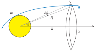
Figure 9: Illustration of a DM particle encounters the Sun. The blue curve represents a trajectory of DM particle (with velocity $\mathbf{u}$ in the solar neighborhood) tangent to the solar surface sphere, with a critical angular momentum $J_{c}=wR_{\odot}$. It is evident that only those with angular momentum below $J_{c}$ can contribute to the encounter rate $\Gamma$. See text for details.

Here we provide a review on the derivation of the rate $\Gamma$ at which the DM flux reaches the solar surface given in Eq. (28). As illustrated in Fig. 9, we imagine a swarm of DM particles from phase space $f_{\chi}\left(\mathbf{u}\right)\mathrm{d}^{3}u$ enters the differential ring area opened by $\mathrm{d}\vartheta$, at a rate of

$$\mathrm{d}\Gamma = \frac{\rho_{\chi}}{m_{\chi}}\,uf_{\chi}\left(\mathbf{u}\right)\mathrm{d}^{3}u\times 2\pi R^{2}\sin\vartheta\cos\vartheta\mathrm{d}\vartheta$$ (37)

$$= \frac{\rho_{\chi}}{m_{\chi}}\,\pi\frac{f_{\chi}\left(\mathbf{u}\right)\mathrm{d}^{3}u}{u}\times\mathrm{d}\left(uR\sin\vartheta\right)^{2}$$

$$= \frac{\rho_{\chi}}{m_{\chi}}\,\pi\frac{f_{\chi}\left(\mathbf{u}\right)\mathrm{d}^{3}u}{u}\times\mathrm{d}J^{2},$$

where the $\mathbf{z}$-axis is by construction parallel to the velocity $\mathbf{u}$, and radius $R$ of an imaginary sphere $S$ is so large that the solar gravitational effect is negligible outside the sphere. Of course, not all of the DM flux entering the ring end up reaching the Sun, but Eq. (37) suggests that angular momentum $J=uR\sin\vartheta$ is a convenient variable in analysis.

Now we calculate the rate at which above DM particle flux reaches the solar surface. First it is straightforward to observe that for those DM particles reach the solar surface with incident velocity $\mathbf{u}$, their speed definitely equals $w=\sqrt{u^{2}+v_{\mathrm{esc}}^{2}\left(R_{\odot}\right)}$, and thus there exists a maximum angular momentum $J_{c}=wR_{\odot}$. That is to say, as the angle $\vartheta$ exceeds a certain critical value, the trajectory of the DM particle will no longer intersect with the solar surface, because a larger angle $\vartheta$ corresponds to a larger angular momentum. This can be equivalently stated in terms of angular momentum: only those DM particles with angular momentum $J\leq wR_{\odot}$ have the chance to enter the Sun.

Although we are discussing the encounter rate of the DM flux with a specific velocity $\mathbf{u}$, the last line in Eq. (37) turns out to be irrelevant of the illustrative $\mathbf{z}$-axis. So for an arbitrary DM velocity $\mathbf{u}$, one can always construct a specific $\mathbf{z}$-axis parallel to this $\mathbf{u}$, repeat the above discussion, and will obtain the same form of differential rate. Therefore, by first integrating over variable $J^{2}$ up to $J_{c}^{2}$ in Eq. (37) and further integrating over the DM velocity $\mathbf{u}$, we obtain the encounter rate in Eq. (28). Moreover, by conservation of the angular momentum, we conclude that $J^{2}$ remains uniform, and the number remains constant per $J^{2}$ interval for the DM particles entering the sphere $S$ and entering the Sun, which helps us determine the injection angle of the DM particles at the solar surface.

References

- (1) SENSEI collaboration, SENSEI: Direct-Detection Results on sub-GeV Dark Matter from a New Skipper-CCD, Phys. Rev. Lett. 125 (2020) 171802 [2004.11378].
- (2) DAMIC-M collaboration, DAMIC-M Experiment: Thick, Silicon CCDs to search for Light Dark Matter, Nucl. Instrum. Meth. A 958 (2020) 162933 [2001.01476].
- (3) SuperCDMS collaboration, Constraints on low-mass, relic dark matter candidates from a surface-operated SuperCDMS single-charge sensitive detector, Phys. Rev. D 102 (2020) 091101 [2005.14067].
- (4) EDELWEISS collaboration, First germanium-based constraints on sub-MeV Dark Matter with the EDELWEISS experiment, Phys. Rev. Lett. 125 (2020) 141301 [2003.01046].
- (5) R. Essig, M. Fernandez-Serra, J. Mardon, A. Soto, T. Volansky and T.-T. Yu, Direct Detection of sub-GeV Dark Matter with Semiconductor Targets, JHEP 05 (2016) 046 [1509.01598].
- (6) Y. Hochberg, Y. Zhao and K. M. Zurek, Superconducting Detectors for Superlight Dark Matter, Phys. Rev. Lett. 116 (2016) 011301 [1504.07237].
- (7) R. Essig, J. Mardon, O. Slone and T. Volansky, Detection of sub-GeV Dark Matter and Solar Neutrinos via Chemical-Bond Breaking, Phys. Rev. D95 (2017) 056011 [1608.02940].
- (8) Y. Hochberg, Y. Kahn, M. Lisanti, C. G. Tully and K. M. Zurek, Directional detection of dark matter with two-dimensional targets, Phys. Lett. B772 (2017) 239 [1606.08849].
- (9) Y. Hochberg, T. Lin and K. M. Zurek, Absorption of light dark matter in semiconductors, Phys. Rev. D95 (2017) 023013 [1608.01994].
- (10) S. Derenzo, R. Essig, A. Massari, A. Soto and T.-T. Yu, Direct Detection of sub-GeV Dark Matter with Scintillating Targets, Phys. Rev. D96 (2017) 016026 [1607.01009].
- (11) Y. Hochberg, Y. Kahn, M. Lisanti, K. M. Zurek, A. G. Grushin, R. Ilan et al., Detection of sub-MeV Dark Matter with Three-Dimensional Dirac Materials, Phys. Rev. D97 (2018) 015004 [1708.08929].
- (12) F. Kadribasic, N. Mirabolfathi, K. Nordlund, A. E. Sand, E. Holmstrom and F. Djurabekova, Directional Sensitivity In Light-Mass Dark Matter Searches With Single-Electron Resolution Ionization Detectors, Phys. Rev. Lett. 120 (2018) 111301 [1703.05371].
- (13) R. Budnik, O. Chesnovsky, O. Slone and T. Volansky, Direct Detection of Light Dark Matter and Solar Neutrinos via Color Center Production in Crystals, Phys. Lett. B782 (2018) 242 [1705.03016].
- (14) S. Knapen, T. Lin, M. Pyle and K. M. Zurek, Detection of Light Dark Matter With Optical Phonons in Polar Materials, Phys. Lett. B785 (2018) 386 [1712.06598].
- (15) S. Griffin, S. Knapen, T. Lin and K. M. Zurek, Directional Detection of Light Dark Matter with Polar Materials, Phys. Rev. D98 (2018) 115034 [1807.10291].
- (16) S. M. Griffin, K. Inzani, T. Trickle, Z. Zhang and K. M. Zurek, Multichannel direct detection of light dark matter: Target comparison, Phys. Rev. D 101 (2020) 055004 [1910.10716].
- (17) T. Trickle, Z. Zhang and K. M. Zurek, Direct Detection of Light Dark Matter with Magnons, 1905.13744.
- (18) N. A. Kurinsky, T. C. Yu, Y. Hochberg and B. Cabrera, Diamond Detectors for Direct Detection of Sub-GeV Dark Matter, Phys. Rev. D99 (2019) 123005 [1901.07569].
- (19) T. Trickle, Z. Zhang, K. M. Zurek, K. Inzani and S. Griffin, Multi-Channel Direct Detection of Light Dark Matter: Theoretical Framework, JHEP 03 (2020) 036 [1910.08092].
- (20) B. Campbell-Deem, P. Cox, S. Knapen, T. Lin and T. Melia, Multiphonon excitations from dark matter scattering in crystals, 1911.03482.
- (21) A. Coskuner, A. Mitridate, A. Olivares and K. M. Zurek, Directional Dark Matter Detection in Anisotropic Dirac Materials, 1909.09170.
- (22) R. M. Geilhufe, F. Kahlhoefer and M. W. Winkler, Dirac Materials for Sub-MeV Dark Matter Detection: New Targets and Improved Formalism, 1910.02091.
- (23) S. M. Griffin, Y. Hochberg, K. Inzani, N. Kurinsky, T. Lin and T. C. Yu, SiC Detectors for Sub-GeV Dark Matter, 2008.08560.
- (24) Z.-L. Liang, L. Zhang, P. Zhang and F. Zheng, The wavefunction reconstruction effects in calculation of DM-induced electronic transition in semiconductor targets, JHEP 01 (2019) 149 [1810.13394].
- (25) N. Kurinsky, D. Baxter, Y. Kahn and G. Krnjaic, Dark matter interpretation of excesses in multiple direct detection experiments, Phys. Rev. D 102 (2020) 015017 [2002.06937].
- (26) J. Kozaczuk and T. Lin, Plasmon production from dark matter scattering, Phys. Rev. D 101 (2020) 123012 [2003.12077].
- (27) S. M. Griffin, K. Inzani, T. Trickle, Z. Zhang and K. M. Zurek, Extended Calculation of Dark Matter-Electron Scattering in Crystal Targets, 2105.05253.
- (28) Y. Hochberg, Y. Kahn, N. Kurinsky, B. V. Lehmann, T. C. Yu and K. K. Berggren, Determining Dark Matter-Electron Scattering Rates from the Dielectric Function, 2101.08263.
- (29) S. Knapen, J. Kozaczuk and T. Lin, Dark matter-electron scattering in dielectrics, 2101.08275.
- (30) D. Baxter, Y. Kahn and G. Krnjaic, Electron Ionization via Dark Matter-Electron Scattering and the Migdal Effect, 1908.00012.
- (31) T. Emken, R. Essig, C. Kouvaris and M. Sholapurkar, Direct Detection of Strongly Interacting Sub-GeV Dark Matter via Electron Recoils, JCAP 1909 (2019) 070 [1905.06348].
- (32) R. Essig, J. Pradler, M. Sholapurkar and T.-T. Yu, On the relation between Migdal effect and dark matter-electron scattering in atoms and semiconductors, 1908.10881.
- (33) M. Heikinheimo, K. Nordlund, K. Tuominen and N. Mirabolfathi, Velocity Dependent Dark Matter Interactions in Single-Electron Resolution Semiconductor Detectors with Directional Sensitivity, Phys. Rev. D99 (2019) 103018 [1903.08654].
- (34) T. Trickle, Z. Zhang and K. M. Zurek, Effective Field Theory of Dark Matter Direct Detection With Collective Excitations, 2009.13534.
- (35) E. Andersson, A. Bökmark, R. Catena, T. Emken, H. K. Moberg and E. Åstrand, Projected sensitivity to sub-GeV dark matter of next-generation semiconductor detectors, JCAP 05 (2020) 036 [2001.08910].
- (36) L. Su, W. Wang, L. Wu, J. M. Yang and B. Zhu, Atmospheric Dark Matter and Xenon1T Excess, Phys. Rev. D 102 (2020) 115028 [2006.11837].
- (37) R. Catena, T. Emken, M. Matas, N. A. Spaldin and E. Urdshals, Crystal responses to general dark matter-electron interactions, 2105.02233.
- (38) G. B. Gelmini, V. Takhistov and E. Vitagliano, Scalar direct detection: In-medium effects, Physics Letters B 809 (2020) 135779.
- (39) S. Knapen, J. Kozaczuk and T. Lin, The Migdal effect in semiconductors, 2011.09496.
- (40) Z.-L. Liang, C. Mo, F. Zheng and P. Zhang, Describing Migdal effect with bremsstrahlung-like process and many-body effects, 2011.13352.
- (41) A. Mitridate, T. Trickle, Z. Zhang and K. M. Zurek, Dark matter absorption via electronic excitations, JHEP 09 (2021) 123 [2106.12586].
- (42) H. An, M. Pospelov, J. Pradler and A. Ritz, Directly Detecting MeV-scale Dark Matter via Solar Reflection, Phys. Rev. Lett. 120 (2018) 141801 [1708.03642].
- (43) Y. Chen, M.-Y. Cui, J. Shu, X. Xue, G.-W. Yuan and Q. Yuan, Sun heated MeV-scale dark matter and the XENON1T electron recoil excess, JHEP 04 (2021) 282 [2006.12447].
- (44) T. Emken, Solar reflection of light dark matter with heavy mediators, 2102.12483.
- (45) P. Giannozzi, S. Baroni, N. Bonini, M. Calandra, R. Car, C. Cavazzoni et al., QUANTUM ESPRESSO: a modular and open-source software project for quantum simulations of materials, Journal of Physics: Condensed Matter 21 (2009) 395502.
- (46) D. R. Hamann, M. Schlüter and C. Chiang, Norm-conserving pseudopotentials, Phys. Rev. Lett. 43 (1979) 1494.
- (47) J. P. Perdew and A. Zunger, Self-interaction correction to density-functional approximations for many-electron systems, Phys. Rev. B 23 (1981) 5048.
- (48) H. J. Monkhorst and J. D. Pack, Special points for brillouin-zone integrations, Phys. Rev. B 13 (1976) 5188.
- (49) A. Marini, C. Hogan, M. Gruning and D. Varsano, yambo: An ab initio tool for excited state calculations, Comput. Phys. Commun. 180 (2009) 1392.
- (50) S. Knapen, J. Kozaczuk and T. Lin, DarkELF: A python package for dark matter scattering in dielectric targets, 2104.12786.
- (51) T. Emken, C. Kouvaris and N. G. Nielsen, The sun as a sub-gev dark matter accelerator, Physical Review D 97 (2018) .
- (52) C. Kouvaris, Probing Light Dark Matter via Evaporation from the Sun, Phys. Rev. D 92 (2015) 075001 [1506.04316].
- (53) T. Lin, Tasi lectures on dark matter models and direct detection, 1904.07915.
- (54) Y. Kahn and T. Lin, Searches for light dark matter using condensed matter systems, 2108.03239.
- (55) J. Kopp, V. Niro, T. Schwetz and J. Zupan, DAMA/LIBRA and leptonically interacting Dark Matter, Phys. Rev. D80 (2009) 083502 [0907.3159].
- (56) A. Gould, Resonant Enhancements in WIMP Capture by the Earth, Astrophys. J. 321 (1987) 571.
- (57) A. Gould, Direct and Indirect Capture of Wimps by the Earth, Astrophys. J. 328 (1988) 919.
- (58) A. Gould, Cosmological density of WIMPs from solar and terrestrial annihilations, Astrophys. J. 388 (1992) 338.
- (59) A. Serenelli, S. Basu, J. W. Ferguson and M. Asplund, New Solar Composition: The Problem With Solar Models Revisited, Astrophys.J. 705 (2009) L123 [0909.2668].
- (60) Z.-L. Liang, Y.-L. Tang and Z.-Q. Yang, The leptophilic dark matter in the Sun: the minimum testable mass, JCAP 10 (2018) 035 [1802.01005].