ResIST: Layer-Wise Decomposition of ResNets for Distributed Training

Chen Dun Computer Science Dept.
Rice University
Houston, Texas, USA
Cameron R. Wolfe Computer Science Dept.
Rice University
Houston, Texas, USA
Christopher M. Jermaine Computer Science Dept.
Rice University
Houston, Texas, USA
Anastasios Kyrillidis Computer Science Dept.
Rice University
Houston, Texas, USA
Abstract

We propose ResIST, a novel distributed training protocol for Residual Networks (ResNets). ResIST randomly decomposes a global ResNet into several shallow sub-ResNets that are trained independently in a distributed manner for several local iterations, before having their updates synchronized and aggregated into the global model. In the next round, new sub-ResNets are randomly generated and the process repeats until convergence. By construction, per iteration, ResIST communicates only a small portion of network parameters to each machine and never uses the full model during training. Thus, ResIST reduces the per-iteration communication, memory, and time requirements of ResNet training to only a fraction of the requirements of full-model training. In comparison to common protocols, like data-parallel training and data-parallel training with local SGD, ResIST yields a decrease in communication and compute requirements, while being competitive with respect to model performance.
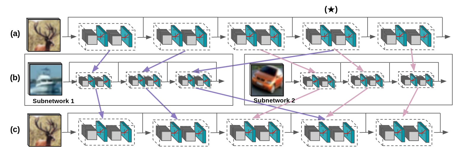
Refer to caption
Figure 1: The ResIST model: Row $\mathbf{(a)}$ represents the original global ResNet. Row $\mathbf{(b)}$ shows the creation of two sub-ResNets. Observe that subnetwork 1 contains the residual blocks #1, #2 and #4, while subnetwork 2 contains the residual blocks #3, #4 and #5. Row $\mathbf{(c)}$ shows the reassembly of the global ResNet, after locally training subnetworks 1 and 2 for some number of local SGD iterations; residual blocks that are common across subnetworks (e.g., residual block #4, marked with a $\star$) are aggregated appropriately during the reassembly.

1 Introduction

Background. The field of Computer Vision (CV) has seen a revolution, beginning with the introduction of AlexNet during the ILSVRC2012 competition. Following this initial application of deep convolutional neural networks (CNNs), the introduction of the residual connection (ResNets) allowed scaling to massive depths without being crippled by issues of unstable gradients during training [He etย al., 2016b]. The capabilities of ResNets have been further expanded in recent years, but the basic ResNet architecture has remained widely-used. While ResNets have become a standard building block for the advancement of CV research, the computational requirements for training them are significant. For example, training a ResNet50 on ImageNet with a single NVIDIA M40 GPU takes 14 days [You etย al., 2018].

Distributed training with multiple GPUs is commonly adopted to speed up the training process for ResNets. Yet, such acceleration is achieved at the cost of a remarkably large number of GPUs (e.g 256 NVIDIA Tesla P100 GPU in [Goyal etย al., 2017]). Additionally, frequent synchronization and high communication costs create bottlenecks that hinder such methods from achieving speedups with respect to the number of available GPUsย [Shi etย al., 2018]. Asynchronous approaches avoid the cost of synchronization, but stale updates complicate their optimization process [Assran etย al., 2020]. Other methods, such as data-parallel training with local SGD [Stich, 2019, Lin etย al., 2018, Zhang etย al., 2016, McMahan etย al., 2017], reduce the frequency of synchronization. Similarly, model-parallel training has gained in popularity by decreasing the cost of local training between synchronization rounds [Ben-Nun and Hoefler, 2019, Zhu etย al., 2020, Kirby etย al., 2020, Gunther etย al., 2020, Guan etย al., 2019, Chen etย al., 2018a].

This paper. We focus on efficient distributed training of CNNs with residual skip connections. Our proposed methodology accelerates synchronous, distributed training by leveraging ResNet robustness to layer removal [Huang etย al., 2016]. In particular, a group of high-performing subnetworks (sub-ResNets) is created by partitioning the layers of a shared ResNet model to create multiple, shallower sub-ResNets. These sub-ResNets are then trained independently (in parallel) for several iterations before aggregating their updates into the global model and beginning the next iteration. Through the local, independent training of shallow sub-ResNets, this methodology both limits synchronization and communicates fewer parameters per synchronization cycle, thus drastically reducing communication overhead. We name this scheme ResNet Independent Subnetwork Training (ResIST). The contributions of this work are:

  • โ€ข

    We propose a distributed training scheme for ResNets, dubbed ResIST, that partitions the layers of a global model to multiple, shallow sub-ResNets, which are then trained independently between synchronization rounds.

  • โ€ข

    We provide theory that ResIST (based on simple ResNet architectures) converges linearly, up to an error neighborhood, using distributed gradient descent with local iterations. We show that the behavior of ResIST is controlled by the overparameterization parameter $m$, as well as the number of workers $S$ in the distributed setting, the number of local iterations, as well as the depth $H$ of the ResNet architecture. Such findings reflect practical observations that are made in the experimental section.

  • โ€ข

    We perform extensive ablation experiments to motivate the design choices for ResIST, indicating that optimal performance is achieved by i)i) using pre-activation ResNets, ii)ii) scaling intermediate activations of the global network at inference time, iii)iii) sharing layers between sub-ResNets that are sensitive to pruning, and iv)iv) imposing a minimum depth on sub-ResNets during training.

  • โ€ข

    ResIST is shown to achieve high accuracy and time efficiency in all cases. We conduct experiments on several image classification and object detection datasets, including CIFAR10/100, ImageNet, and PascalVOC.

  • โ€ข

    We utilize ResIST to train numerous different ResNet architectures (e.g., ResNet101, ResNet152, and ResNet200) and provide implementations for each in PyTorch [Paszke etย al., 2019].

2 Sub-ResNet Training

ResIST operates by partitioning the layers of a global ResNet to different, shallower sub-ResNets, training those independently, and intermittently aggregating their updates into the global model. The high-level process followed by ResIST is depicted in Fig. 1 and outlined in more detail by Algorithm 1. We note that a naive, uniform partitioning of blocks to each subnetwork, resembling a distributed implementation of [Huang etย al., 2016], performs poorly (see Fig. 6). To improve upon this procedure, extensive design choices, outlined in Section A.1 in the Appendix, are studied to motivate ResIST, leading to a final methodology that generalizes well across domains and datasets.

2.1 Model Architecture

Refer to caption
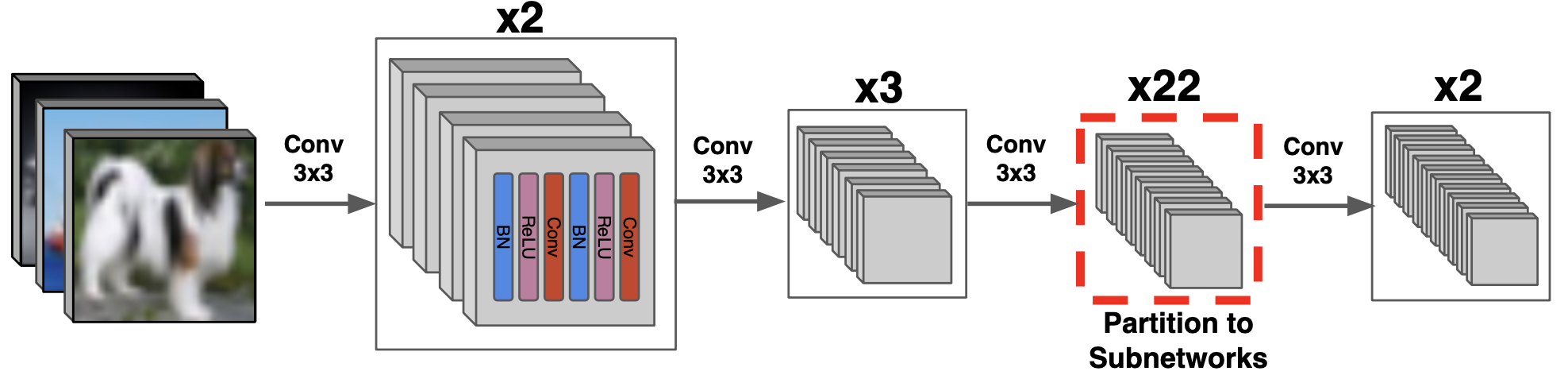
Figure 2: The ResNet101 model used in the majority of experiments. The figure identifies the convolutional blocks that are partitioned to subnetworks. The plot depicts the pre-activation ResNet setting, where we use BN, ReLU, and Conv layers twice in sequence. The network is comprised of four major โ€œsectionsโ€, each containing a certain number of convolutional blocks of equal channel dimension.

To achieve optimal performance with ResIST, the global model must be sufficiently deep. Otherwise, sub-ResNets may become too shallow after partitioning, leading to poor performance. For most experiments, a ResNet101 architecture is selected, which balances sufficient depth with reasonable computational complexity. Experiments with deeper architectures are provided in Section A.4 in the Appendix.

ResIST performs best with pre-activation ResNets [He etย al., 2016a]. Intuitively, applying batch normalization prior to the convolution ensures that the input distribution of remaining residual blocks will remain fixed, even when certain layers are removed from the architecture. The Pre-activation ResNet101, which we utilize for the majority of experiments, is depicted in Fig. 2. This model, as well as deeper variants (e.g., ResNet152 and ResNet200), are readily available through deep learning packages like PyTorch [Paszke etย al., 2019] and Tensorflow [Abadi etย al., 2015].

2.2 Sub-ResNet Construction

Pruning literature has shown that strided-, initial-, and final-layers within CNNs are sensitive to pruning [Li etย al., 2017]. Additionally, repeated blocks of identical convolutions (i.e., equal channel size and spatial resolution) are less sensitive to pruning [Li etย al., 2017]. Drawing upon these results, ResIST only partitions blocks within the third section of the ResNet (see the highlighted section in Fig. 2), while all other blocks are shared between sub-ResNets. These blocks are chosen for partitioning because $i)$ they account for the majority of layers; $ii)$ they are not strided; $iii)$ they are located within the middle of the network (i.e., initial/final layers are excluded); and $iv)$ they reside within a long chain of identical convolutions. By partitioning these blocks, ResIST allows sub-ResNets to be shallower than the global model, while maintaining high performance.

The process of constructing sub-ResNets follows a simple procedure; see Figure 1. From row $(a)$ to $(b)$ within Figure 1, indices of partitioned layers within the global model are randomly permuted and distributed to sub-ResNets in a round-robin fashion. Each sub-ResNet receives an equal number of convolutional blocks (e.g., see row $(b)$). In cases, residual blocks may be simultaneously partitioned to multiple sub-ResNets to ensure sufficient depth (e.g., see $(\star)$ in Figure 1). ResIST produces subnetworks with $\mathcal{O}(\frac{1}{S})$ of the global model depth, where $S$ is the number of independently-trained sub-ResNets.111A fixed number of blocks is excluded from partitioning (i.e., blocks not in the third section). As a result, this approximation of $\mathcal{O}(\frac{1}{S})$ becomes more accurate as the network becomes deeper (i.e., deeper ResNet variants only add blocks to the third section), as a larger ratio of total blocks are included in the partitioning process. To contrast this with existing non-distributed attempts, stochastic depth networks [Huang etย al., 2016] have an expected depth of 75% of the global model.

The shallow sub-ResNets created by ResIST accelerate training and reduce communication in comparison to methods that communicate and train the full model. Table 1 shows the comparison of local SGD to ResIST with respect to the amount of data communicated during each synchronization round for different numbers of machines, highlighting the superior communication-efficiency of ResIST.

Table 1: Data communicated during each communication round (in GB) of both local SGD [Stich, 2019] and ResIST across different numbers of machines with ResNet101.
Method 2 Machine 4 Machine 8 Machine
Local SGD 0.662 GB 1.325 GB 2.649 GB
ResIST 0.454 GB 0.720 GB 1.289 GB

2.3 Distributed Training

The ResIST training procedure is outlined in Algorithm 1. Sub-ResNet construction (i.e., subResNets$(\cdot)$ in Algorithm 1) follows the procedure outlined in Sec. 2.2. After constructing the sub-ResNets, they are trained independently in a distributed manner for $\ell$ iterations. Following independent training, the updates from each sub-ResNet are aggregated into the global model. Aggregation (i.e., $\text{{aggregate}}(\cdot)$ in Algorithm 1) sets each global network parameter to its average value across the sub-ResNets to which it was partitioned. If a parameter is only partitioned to a single sub-ResNet, aggregation simplifies to copying the parameter into the global model. After aggregation, the global model is re-partitioned randomly to create a new group of sub-ResNets, and this entire process is repeated.

Algorithm 1 ResIST Meta Algorithm
ย ย Parameters: $T$ synchronization iterations, $S$ sub-ResNets, $\ell$ local iterations, $\mathcal{W}$ ResNet weights.
ย ย hโ€‹(๐’ฒ)โ„Ž๐’ฒh(\mathcal{W}) $\leftarrow$ randomly initialized ResNet.
ย ย forย t=0,โ€ฆ,Tโˆ’1๐‘ก0โ€ฆ๐‘‡1t=0,\dots,T-1ย do
ย ย ย ย ย {hsโ€‹(Ws)}s=1S=subResNetsโ€‹(hโ€‹(W),S)superscriptsubscriptsubscriptโ„Ž๐‘ subscript๐‘Š๐‘ ๐‘ 1๐‘†subResNetsโ„Ž๐‘Š๐‘†\left\{h_{s}(W_{s})\right\}_{s=1}^{S}=\text{{subResNets}}(h(W),\leavevmode\nobreak\ S).
ย ย ย ย ย Distribute each hsโ€‹(Ws)subscriptโ„Ž๐‘ subscript๐‘Š๐‘ h_{s}(W_{s}) to a different worker.
ย ย ย ย ย forย s=1,โ€ฆ,S๐‘ 1โ€ฆ๐‘†s=1,\dots,Sย do
ย ย ย ย ย ย ย ย //ย Train hsโ€‹(Ws)subscriptโ„Ž๐‘ subscript๐‘Š๐‘ h_{s}(W_{s}) for $\ell$ iterations using local SGD.
ย ย ย ย ย ย ย ย forย lt=1,โ€ฆ,โ„“subscript๐‘™๐‘ก1โ€ฆโ„“l_{t}=1,\dots,\ellย do
ย ย ย ย ย ย ย ย ย ย ย Ws=Wsโˆ’ฮทโ€‹โˆ‚LWssubscript๐‘Š๐‘ subscript๐‘Š๐‘ ๐œ‚๐ฟsubscript๐‘Š๐‘ W_{s}=W_{s}-\eta\frac{\partial L}{W_{s}}
ย ย ย ย ย ย ย ย endย for
ย ย ย ย ย endย for
ย ย ย ย ย hโ€‹(๐’ฒ)=aggregateโ€‹({hsโ€‹(Ws)}s=1S)โ„Ž๐’ฒaggregatesuperscriptsubscriptsubscriptโ„Ž๐‘ subscript๐‘Š๐‘ ๐‘ 1๐‘†h(\mathcal{W})=\texttt{aggregate}\left(\left\{h_{s}(W_{s})\right\}_{s=1}^{S}\right).
ย ย endย for
Refer to caption
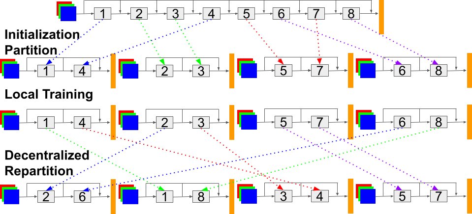
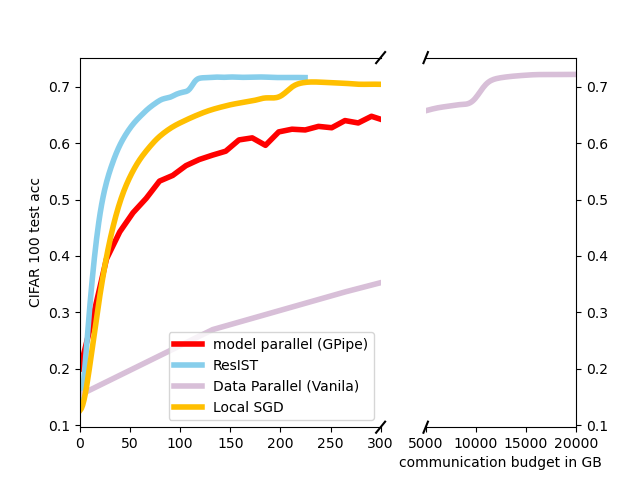
Figure 3: A depiction of the decentralized repartition procedure. This example partitions a ResNet with eight blocks into four different sub-ResNets. The โ€œblue-green-redโ€ squares dictate the data that lies per worker; the orange column dictates the last classification layer. As seen in the figure, each worker is responsible for only a fraction of parameters of the whole network. The whole ResNet is never fully stored, communicated or updated on a single worker.
Refer to caption
Figure 4: Communication efficiency of ResIST versus data parallelism (vanila), model parallelism (GPipe - [Huang etย al., 2019]) and local SGD (LSGD) on CIFAR100.

2.4 Baseline Choice

Common baselines for distributed training are generally split into data- and model-parallelism protocols. Focusing on the former, the communication efficiency of ResIST significantly surpasses data-parallelism. In particular, data parallel methods need to synchronize the whole model at every training iteration, while ResIST only needs to communicate the weights of sub-ResNets among the workers.

Typically, model parallel techniques split the model into modules (such as layers) and distribute these modules to each worker. At every training iteration, input data is first passed to the worker containing the networkโ€™s beginning module (e.g., the first layer). Then, at each module, the worker $i)$ performs a forward pass of its module and $ii)$ sends the resulting output activation to the worker containing the next module. After the last module is activated, the final loss and gradient is calculated before the backward pass is performed, where each worker receives gradient information needed for updating module weights.

Model-parallelism often suffers from higher communication frequency and volume, in comparison to data parallel methods, due to the significant cost of transmitting network activation maps between workers. E.g., model parallel training of ResNets requires transmission of the full batch activation map between layers, which is more cumbersome than simply communicating network parameters. ResIST is more communication efficient compared to common model parallel methods (e.g., GPipe [Huang etย al., 2019]).

Within this work, we adopt local SGD [Lin etย al., 2018]โ€”a strong variant of data parallel trainingโ€”as our baseline. Similar to ResIST, local SGD performs local training iterations on each worker between synchronizations, thus largely decreasing communication frequency and volume. To justify this selection, we perform a baseline comparison, which is displayed in Figure 4 and further detailed in Sections 2.5 and 5. As shown in Figure 4, ResIST is significantly more communication efficient in comparison to data-parallelism (vanilla) and model-parallelism (GPipe), thus making local SGD a more appropriate baseline.

2.5 Implementation Details

ResIST is implemented in PyTorch [Paszke etย al., 2019], using the NCCL communication package. We use basic broadcast and reduce operations for communicating blocks in the third section and all reduce for blocks in other sections. We adopt the same communication procedure for the local SGD baseline to ensure fair comparison. The implementation of ResIST is decentralized, meaning that it does not assume a single, central parameter server.

As shown in Figure 3, during the synchronization and repartition step following local training, each sub-ResNet will directly send each of its locally-updated blocks to the designated new sub-ResNet. Each worker will only need sufficient memory to store a single sub-ResNet, thus limiting the memory requirements. Such a decentralized implementation allows parallel communication between sub-ResNets, which leads to further speedups by preventing any single machine from causing slow-downs due to communication bottlenecks. The implementation is easily scalable to eight or more machines, either on nodes with multiple GPUs or across distributed nodes with dedicated GPUs.

ResIST reduces the number of bits communicated at each synchronization round and accelerates local training with the use of shallow sub-ResNets. The authors are well-aware of many highly-optimized versions of data-parallel and synchronous training methodologies [Paszke etย al., 2019, Abadi etย al., 2015, Sergeev and Delย Balso, 2018]. ResIST is fully compatible with these frameworks and can be further accelerated by leveraging highly-optimized distributed communication protocols at the systems level, which we leave as future work. Further, the authors are well-aware of advanced recent decentralized distributed computing techniques as in [Koloskova etย al., 2020, Nedic and Ozdaglar, 2009, Assran and Rabbat, 2020, Koloskova etย al., 2019]; our aim is to show the benefits of our approach even on simpler distributed frameworks, and we leave the extension of ResIST to such more advanced protocols as future work.

2.6 Supplemental Techniques

Scaling Activations. Similar to [Huang etย al., 2016], activations must be scaled appropriately to account for the full depth of the resulting network at test time. To handle this, the output of residual blocks in the third section of the network (see Figure 2) is scaled by $1/S$, where $S$ is the number of sub-ResNets. Such scaling allows the global model to perform well, despite using all layers at test time.

Subnetwork Depth. Within ResIST, sub-ResNets may become too shallow as the number of sub-ResNets increases. To solve this issue, ResIST enforces a minimum depth requirement, which is satisfied by sharing certain blocks between multiple sub-ResNets. Through experimental analysis, a minimum of five blocks partitioned to each sub-ResNet was found to perform optimally. Such a finding motivates our choice of the ResNet101 architecture, as ResNet50 contains only five blocks for partitioning. ResIST is extensible to deeper architectures; see Section A.4 in the Appendix.

Tuning Local Iterations. We use a default value of $\ell=50$, as $\ell<50$ did not noticeably improve performance. In some cases, the performance of ResIST can be improved by tuning $\ell$ (see Figure 7). The optimal $\ell$ setting in ResIST is further explored in Section A.3 in the Appendix.

Local SGD Warm-up Phase. Directly applying ResIST may harm performance on some large-scale datasets (e.g., ImageNet). To resolve this, we perform a few epochs with data parallel local SGD before training the model with ResIST.222Activations of blocks within $3^{\text{rd}}$ section are still scaled during local SGD pre-training to maintain consistency with ResIST. By simply pre-training a model for a few epochs with local SGD, the remainder of training is completed using ResIST without a significant performance decrease.

3 Theoretical Result

We provide proof that the gradient descent direction of combined updates from all sub-ResNets, during distributed local training, is close to the hypothetical gradient descent direction of the whole model as if trained centrally.

Theorem 3.1 (Convergence Rate of Gradient Descent for ResIST).

Assume there are $S$ workers, $\ell$ local and $T$ global steps. Assume the depth of the whole ResNet is $H$. Assume for all data indices $i\in[n]$, the data input satisfies $\left\|\mathbf{x}_{i}\right\|_{2}=1$, the data output satisfies $\left|y_{i}\right|=O(1)$, and the number of hidden nodes per layer satisfies $m=$

$\displaystyle\Omega\bigg{(}\max\bigg{\{}\tfrac{n^{4}}{\lambda_{\min}^{4}\left(\mathbf{K}^{(H)}\right)H^{6}},\tfrac{n^{2}}{\lambda_{\min}^{2}(\mathbf{K}^{(H)})H^{2}},\tfrac{n}{\delta},\tfrac{n^{2}\log\left(\tfrac{Hn}{\delta}\right)}{\lambda_{\min}^{2}\left(\mathbf{K}^{(H)}\right)}\bigg{\}}\bigg{)}.$

Set the step size $\eta=O\bigg{(}\tfrac{\lambda_{\min}\left(\mathbf{K}^{(H)}\right)H^{2}}{n^{2}\ell^{2}S}\bigg{)}$ in gradient descent in local training iteration, and follow the procedure as in Algorithm 1. Let the squared-norm loss be $L(\theta(t)):=\tfrac{1}{2}\|\mathbf{y}-f(\theta(t))\|_{2}^{2}$, per $t$ global synchronization round, $t=1,2,\ldots T$; here, $\mathbf{y}$ corresponds to the data โ€œlabelsโ€, and $\theta(t)$ and $f(\theta(t))$ represent the parameters and the output of the whole ResNet, respectively, after $t$-global rounds of ResIST. Here, $\theta$ includes weights $\mathbf{W}^{(h)}$ at depth $h$ and the last layerโ€™s weights $\mathbf{a}$. Then, with probability at least $1-\delta$ over the random initialization, we have:

$\displaystyle L(\mathbf{\theta}(t))\leq\left(1-\tfrac{\eta\ell\lambda_{\min}\left(\mathbf{K}^{(H)}\right)}{2}\right)^{t}\cdot L(\mathbf{\theta}(0)).$

First, some definitions; more details in the Appendix. Similar to [Du etย al., 2019], $\mathbf{K}^{(H)}\in\mathbb{R}^{n\times n}$ is a fixed matrix that depends on the input data, neural network architecture and the activation but does not depend on neural network parameters. Next, we present our method of proving this global result on ResIST. Our proof technique is inspired by [Du etย al., 2019]: Let the prediction of the network at some $k$-th iteration be $\mathbf{u}(k)=f(\theta(k))$.333We use $k$ to abstract the notion of an iteration in [Du etย al., 2019]; in our case, a different analysis includes two different iteration indices, $\ell$ and $t$. We formulate the training dynamics as:

$\displaystyle\mathbf{y}-\mathbf{u}(k+1)=(\mathbf{I}-\eta\mathbf{G}(k))(\mathbf{y}-\mathbf{u}(k)),$

where $\mathbf{G}_{ij}(k)=\left\langle\frac{\partial u_{i}(k)}{\partial\mathbf{\theta}(k)},\frac{\partial u_{j}(k)}{\partial\mathbf{\theta}(k)}\right\rangle=$

$\displaystyle\sum_{h=1}^{H}\left\langle\tfrac{\partial u_{i}(k)}{\partial\mathbf{W}^{(h)}(k)},\tfrac{\partial u_{j}(k)}{\partial\mathbf{W}^{(h)}(k)}\right\rangle+\left\langle\tfrac{\partial u_{i}(k)}{\partial\mathbf{a}(k)},\tfrac{\partial u_{j}(k)}{\partial\mathbf{a}(k)}\right\rangle$
$\displaystyle\triangleq$ $\displaystyle\sum_{h=1}^{H+1}\mathbf{G}^{(h)}_{ij}(k).$

The proof in [Du etย al., 2019] obeys the following ideas: when the width $m$ of deep ResNet is sufficiently large, $\mathbf{G}^{(H)}(k)$ will be very close to $\mathbf{G}^{(H)}(0)$, and all of $\mathbf{G}^{(H)}(k)$โ€™s will be close to the fixed population gram matrix $\mathbf{K}^{(H)}$. The exact definition of $\mathbf{K}^{(H)}$ for ResNet can be found in Section 6 of Du etย al. [2019]. Further, $\lambda_{\min}(\mathbf{G}^{(H)}(0))$ is larger than 0. Thus, by standard matrix perturbation analysis, it is shown that $\lambda_{\min}(\mathbf{G}^{(H)}(0))$ is also strictly positive, which will result in linear convergence of deep ResNet.

Here, we further generalize such technique to distributed ResIST with layer dropout. The novelty of our proof is that we only conduct gradient descent on sub-ResNets assigned to each local worker. There is no training iteration with the whole model: this includes the generation of random masks that โ€œchampionโ€ parts of the whole ResNet model per worker. Handling such constructions is the gist of this proof: We carefully analyze the convergence of each subnetwork during local training iterations $\ell$, and prove the global convergence of the combined whole model throughout synchronization rounds $t$. The full proof is provided in Section B in the Appendix.

4 Related Work

Following ResNet, most novel architectures continued to leverage residual connections, which became standard in most architectures. The ResNet architecture has been further modified. This work focuses on the pre-activation ResNet variant [He etย al., 2016a], as it achieves high performance and is well-suited to layer-wise decomposition.

The focus of this study is on synchronous methods of distributed optimization, such as data parallel training, parallel SGD [Zinkevich etย al., 2010], or local SGD [Stich, 2019]. Our methodology is also a variant of model-parallel training [Ben-Nun and Hoefler, 2019, Zhu etย al., 2020, Kirby etย al., 2020, Gunther etย al., 2020, Guan etย al., 2019, Chen etย al., 2018a]. Many studies have explored possible techniques of synchronous, distributed optimization, yielding a wide number of viable variants [Lin etย al., 2018].

To reduce communication costs in the distributed setting, both quantization [Alistarh etย al., 2017, Tang etย al., 2018] and sparsification [Aji and Heafield, 2017, Jiang and Agrawal, 2018, Wangni etย al., 2018] methods have been explored. Similarly, other studies have achieved speedups through the use of low-precision arithmetic during training [Jia etย al., 2018]. However, this line of work is orthogonal to our proposal and can be easily combined with the provided methodology; see Section A.5 in the Appendix.

Large batch training is used to amortize communication and increase throughput for distributed training [Goyal etย al., 2017, You etย al., ]. The properties of large batch training have since been studied extensively [Akiba etย al., 2017, You etย al., 2017, 2018]. Large batches alter training dynamics, warranting the use of complex heuristics to maintain comparable performance [You etย al., 2017]. Here, we do not focus on the extension of ResIST to the large-batch training domain. Rather, we consider this as future work.

ResNet robustness to layer removal was explored in [Huang etย al., 2016], while [Veit etย al., 2016] showed that ensembles of shallow ResNets can yield high performance. [Huang etย al., 2016] uses shallow networks during training and scales activations so that all layers may be used for inference. However, our approach is distinct in numerous ways. Primarily, our method partitions blocks in a stochastic, round-robin fashion, which explicitly prevents the exclusion of layers from training rounds and yields reduced subnetwork depth compared to [Huang etย al., 2016]. Inspired by [Li etย al., 2017], we also selectively partition residual blocks that are least sensitive to pruning, allowing other layers (i.e., ย 30% of total layers) to be shared between subnetworks. Unlike [Huang etย al., 2016], we avoid partitioning strided layers, which are sensitive to pruning [Li etย al., 2017]. Furthermore, our methodology, instead of proposing a form of regularization, focuses on utilizing independent training of shallow sub-ResNets for efficient, distributed training.

Our approach also relates to neural ODE literature. This research connects ResNets as a discrete approximation to a continuous transformation from input to output [Lu etย al., 2018]. The neural ODE perspective has been studied both empirically [Chen etย al., 2018b, Dupont etย al., 2019, Lu etย al., 2018] and theoretically [Lu etย al., 2020, Thorpe and van Gennip, 2018]. This provides justification to our approach, as removing ResNet layers can be viewed as approximating the same transformation with a coarser discretization.

5 Experimental Details

Hyperparameters are tuned using a holdout validation set and results are obtained using optimal hyperparameters from the validation set. All experiments are repeated for three trials, and the average performance is presented. We adopt local SGD as our baseline for synchronous, distributed training methods. In all cases, ResIST achieves comparable performance to local SGD, while lowering the total wall-clock time of training. We use AWS p3.8xlarge instances for experiments with two or four machines444In Section A.4-Appendix and for the Pacal VOC experiment with two machines, we use a cluster with eight V100 GPUs. and p3.16xlarge instances for experiments with eight machines. We use each GPU as a single worker that hosts a different sub-ResNet.

Small-Scale Image Classification. Models are trained with ResIST on CIFAR10 and CIFAR100 for image classification. We adopt standard data augmentation techniques during training and testing [He etย al., 2016b]. We adopt a batch size of 128 for each worker. Training is conducted for 80 epochs for experiments with two machines and 160 epochs for experiments with four or eight machines. The recorded performance reflects the best test accuracy achieved throughout training, averaged across three trials. The total wall-clock training time is also reported for each experiment.

ImageNet Classification. Models are trained with ResIST on the 1,000-class ILSVRC2012 image classification dataset [Deng etย al., 2009]. We adopt standard data augmentation techniques during training and testing, and use a batch size of 256 for each worker [He etย al., 2016b]. Training is conducted for 90 epochs. We initialize the learning rate to 0.1 and decrease it $10\times$ at epochs 30 and 60. For all experiments, we set $\ell=15$, adopt a minimum depth of 10 blocks for each sub-ResNet, and warm-up pre-training using local SGD. For both ResIST and baseline experiments, we utilize momentum restarts and aggregate batch statistics every 1300 synchronization rounds.

Object Detection. ResIST is tested in the object detection domain on the Pascal VOC dataset [Everingham etย al., 2010]. Our model, inspired by the Yolo-v2 object detection model [Redmon and Farhadi, 2017], consists of a ResNet101 backbone followed by a detection layer (i.e., a $1\times 1$ convolution that outputs anchor box predictions). The ResNet backbone of this model is similar to the classification model described in Sec. 2.1, but without the pre-activation structure. The model is trained for 100 epochs with an image dimension of $448\times 448$ and batch size of 10. No data augmentation techniques are used. The learning rate is increased from $10^{-5}$ to $10^{-4}$ over the first 30 epochs, and decreased by $10\times$ at epochs 60 and 90. Both Pascal VOC 2007 and 2012 training sets are used during training, and performance is evaluated on the Pascal VOC 2007 test set. We report the wall-clock training time and the best loss achieved on the test set throughout training. Experiments are conducted on two and four machines using both local SGD and ResIST.

Table 2: Test accuracy of baseline LocalSGD versus ResIST on small-scale image classification datasets.
# Machines CIFAR10 CIFAR100
Local SGD 2 92.36% $\pm$ 0.01 70.67% $\pm$ 0.03
4 92.90% $\pm$ 0.06 71.51% $\pm$ 0.04
8 92.00% $\pm$ 0.07 69.64% $\pm$ 0.05
ResIST 2 91.95% $\pm$ 0.32 70.06% $\pm$ 0.51
4 92.35% $\pm$ 0.22 71.30% $\pm$ 0.20
8 91.45% $\pm$ 0.30 70.26% $\pm$ 0.21

6 Results

6.1 Small-Scale Image Classification

Table 3: Performance of baseline models and models trained with ResIST on 1K Imagenet [Recht etย al., 2019]. MF stands for test set โ€œMatchedFrequencyโ€ and was sampled to match the MTurk selection frequency distribution of the original ImageNet validation set; T-0.7 stands for test set โ€œThreshold0.7โ€ and was built by sampling ten images for each class among the candidates with selection frequency at least 0.7; TI stands for test set โ€œTopImagesโ€ and contains the ten images with highest selection frequency for each class.
# Machines Imagenet Imagenet V2 Test Set Training Time Speedup Communication Cost Ratio
MF T-0.7 TI
Local SGD 2 73.32% 60.72% 69.47% 75.48% 48.61 hours - 7546.80 GB -
4 72.66% 59.88% 68.34% 74.27% 29.29 hours - 7546.80 GB -
ResIST 2 71.60% 58.92% 67.51% 73.56% 36.79 hours 1.32$\times$ 5831.2 GB 1.29$\times$
4 70.74% 57.56% 66.46% 72.65% 22.37 hours 1.31$\times$ 6007.6 GB 1.26$\times$

Accuracy. The test accuracy on small-scale image classification datasets is listed in Table 2. ResIST achieves comparable test accuracy in all cases where the same number of machines are used. ResIST outperforms localSGD on CIFAR100 experiments with eight machines. The performance of ResIST and local SGD are strikingly similar in terms of test accuracy. In fact, the performance gap between the two method does not exceed 1% in any experimental setting. Furthermore, ResIST performance remains stable as the number of sub-ResNets increases, allowing greater acceleration to be achieved without degraded performance (e.g., see CIFAR100 results in Table 2). Generally, using four sub-ResNets yields the best performance with ResIST.

Efficiency. In addition to achieving comparable test accuracy, ResIST significantly accelerates training. This acceleration is due to $i)$ fewer parameters being communicated between machines and $ii)$ locally-trained sub-ResNets being shallower than the global model. Wall-clock training times for four and eight machine experiments are presented in Tables 4. ResIST provides $3.58$ to $3.81\times$ speedup in comparison to local SGD. For eight machine experiments, a significant speedup over four machine experiments is not observed due to the minimum depth requirement and a reduction in the number of local iterations to improve training stability. We conjecture that for cases with higher communication cost at each synchronization and a similar number of synchronizations, eight worker ResIST could lead to more significant speedups in comparison to the four worker case.

Table 4: Training time in seconds of baseline models and models trained with ResIST on small-scale image classification datasets.
# Machines Dataset Total Time Speedup
Local SGD 4 C10 5486 $\pm$ 7.05 -
C100 5528 $\pm$ 65.90 -
8 C10 10072 $\pm$ 5.12 -
C100 10058 $\pm$ 8.71 -
ResIST 4 C10 1532 $\pm$ 0.83 3.60$\times$
C100 1545 $\pm$ 1.27 3.58$\times$
8 C10 2671 $\pm$ 3.25 3.77$\times$
C100 2639 $\pm$ 3.89 3.81$\times$
Refer to caption
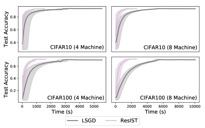
Figure 5: Both methodologies complete 160 epochs of training. Accuracy values are smoothed using a 1-D gaussian filter, and shaded regions represent deviations in accuracy.

A visualization of the speedup provided by ResIST on the CIFAR10 and CIFAR100 datasets is illustrated in Fig. 5. Models trained with ResIST match the final accuracy of those trained with local SGD. Furthermore, increasing the number of sub-ResNets yields an improved speedup for ResIST in comparison to localSGD. It is clear that the communication-efficiency of ResIST allows the benefit of more devices to be better realized in the distributed setting.

6.2 Large-Scale Image Classification

Accuracy. The test accuracy of models trained with both ResIST and local SGD for different numbers of machines on the ImageNet dataset is listed in Table 3. As can be seen, ResIST achieves comparable test accuracy ($<2\%$ difference) to local SGD in all cases. Additionally, as shown in [Recht etย al., 2019], many current image classification models overfit to the ImageNet test set and cannot generalize well to new data. Thus, models trained with both local SGD and ResIST are also evaluated on three different Imagenet V2 testing sets [Recht etย al., 2019]. As shown in Table 3, ResIST consistently achieves comparable test accuracy in comparison to local SGD on these supplemental test sets.

Efficiency. As shown in Tables 3 and 5, ResIST significantly accelerates the ImageNet training process. However, due to the use of fewer local iterations and the local SGD warm-up phase, the speedup provided by ResIST is smaller relative to experiments on small-scale datasets. In Table 3, ResIST can reduce the total communication volume during training, which is an important feature in the implementation of distributed systems with high computational costs.

Table 5: Total training time on Imagenet (in hours) of models trained with both local SGD and ResIST using two and four machines to reach a fixed test accuracy.
# Machines Target Accuracy Local SGD ResIST Speedup
2 71.00 33.26 26.63 1.25$\times$
4 70.70 18.50 18.12 1.02$\times$

6.3 Object Detection

Loss. The test loss of models trained with both ResIST and local SGD for different numbers of machines on the Pascal VOC object detection dataset is listed in Table 6. Notably, ResIST achieves a lower test loss in comparison to local SGD for the experiment with two machines. Although the test loss achieved by ResIST is slightly worse than local SGD in the four machine case, the performance is comparable. Namely, the difference in test loss achieved by local SGD and ResIST never exceeds a value of one.

Efficiency. In addition to achieving comparable or improved test loss in comparison to local SGD, ResIST also provides a significant training acceleration on the PascalVOC dataset. In particular, models trained with ResIST achieve up to a $1.64\times$ acceleration in comparison to object detection models trained with localSGD.

Table 6: Test loss and total training time in seconds on Pascal VOC for models trained with both local SGD and ResIST using two and four machines. Training time in seconds.
# Machines Test Loss Train Time Speedup
Local SGD 2 6.15 $\pm$ 0.03 39621 $\pm$ 9.12 -
4 6.22 $\pm$ 0.06 16840 $\pm$ 0.11 -
ResIST 2 5.99 $\pm$ 0.01 24058 $\pm$ 3.22 1.64$\times$
4 6.69 $\pm$ 0.17 11264 $\pm$ 49.38 1.49$\times$

6.4 More experiments

In the Appendix A, we outline numerous ablation experiments that were performed using ResIST. These experiments provide an understanding of the algorithmโ€™s behavior, as well as empirical support for its design: they include ResIST design decisions (Section A.1), comparison of ResIST with ensemble methods (Section A.2), robustness to local iterations (Section A.3), applicability of ResIST to deeper architectures (Section A.4), and compatibility to existing quantization/sparsification techniques (Section A.5).

7 Conclusion

In the work, we present ResIST, a novel algorithm for synchronous, distributed training of ResNets. ResIST operates by decomposing a global ResNet model into several shallower sub-ResNets, which are trained independently and itermittently aggregated into the global model. By only communicating parameters of sub-ResNets between machines and training shallower, less expensive networks, ResIST reduces the communication and local training cost of synchronous, distributed training. We demonstrate the impact of ResIST on several image classification datasets, as well as in the object detection domain, by highlighting the significant training acceleration it provides in comparison to methods like local SGD [Lin etย al., 2018] without any deterioration in performance.

We aim to extend ResIST to other network architectures, as ResIST is fully-extensible to all network architectures with residual connections. Because residual connections are now standard in most important deep learning architectures (e.g., transformers), many opportunities to extend applications of ResIST exist. On the other hand, ResIST has been shown to be fully-compatible with various gradient compression methods. As such, we will investigate the prospect of fully integrating such compression methods within ResIST, both during training and communication phases, to further decrease memory and computation costs.

References

  • Abadi etย al. [2015] Martรญn Abadi etย al. TensorFlow: Large-scale machine learning on heterogeneous systems, 2015.
  • Aji and Heafield [2017] Alhamย Fikri Aji and Kenneth Heafield. Sparse communication for distributed gradient descent. In Proceedings of the 2017 Conference on Empirical Methods in Natural Language Processing, pages 440โ€“445, 2017.
  • Akiba etย al. [2017] Takuya Akiba, Shuji Suzuki, and Keisuke Fukuda. Extremely large minibatch SGD: Training ResNet-50 on imagenet in 15 minutes. arXiv:1711.04325, 2017.
  • Alistarh etย al. [2017] Dan Alistarh, Demjan Grubic, Jerry Li, Ryota Tomioka, and Milan Vojnovic. QSGD: Communication-efficient SGD via gradient quantization and encoding. Advances in Neural Information Processing Systems, 30, 2017.
  • Assran etย al. [2020] Mahmoud Assran, Arda Aytekin, Hamidย Reza Feyzmahdavian, Mikael Johansson, and Michaelย G Rabbat. Advances in asynchronous parallel and distributed optimization. Proceedings of the IEEE, 108(11):2013โ€“2031, 2020.
  • Assran and Rabbat [2020] Mahmoudย S Assran and Michaelย G Rabbat. Asynchronous gradient push. IEEE Transactions on Automatic Control, 66(1):168โ€“183, 2020.
  • Ben-Nun and Hoefler [2019] Tal Ben-Nun and Torsten Hoefler. Demystifying parallel and distributed deep learning: An in-depth concurrency analysis. ACM Computing Surveys (CSUR), 52(4):1โ€“43, 2019.
  • Chen etย al. [2018a] Chi-Chung Chen, Chia-Lin Yang, and Hsiang-Yun Cheng. Efficient and robust parallel dnn training through model parallelism on multi-gpu platform. arXiv preprint arXiv:1809.02839, 2018a.
  • Chen etย al. [2018b] Rickyย TQ Chen, Yulia Rubanova, Jesse Bettencourt, and Davidย K Duvenaud. Neural ordinary differential equations. Advances in neural information processing systems, 31, 2018b.
  • Deng etย al. [2009] Jia Deng, Wei Dong, Richard Socher, Li-Jia Li, Kai Li, and Liย Fei-Fei. Imagenet: A large-scale hierarchical image database. In 2009 IEEE conference on computer vision and pattern recognition, pages 248โ€“255. Ieee, 2009.
  • Du etย al. [2019] Simon Du, Jason Lee, Haochuan Li, Liwei Wang, and Xiyu Zhai. Gradient descent finds global minima of deep neural networks. In International conference on machine learning, pages 1675โ€“1685. PMLR, 2019.
  • Dupont etย al. [2019] Emilien Dupont, Arnaud Doucet, and Yeeย Whye Teh. Augmented neural ODEs. In Advances in Neural Information Processing Systems, pages 3140โ€“3150, 2019.
  • Everingham etย al. [2010] Mark Everingham, Luc Vanย Gool, Christopherย KI Williams, John Winn, and Andrew Zisserman. The pascal visual object classes (VOC) challenge. International journal of computer vision, 88(2):303โ€“338, 2010.
  • Goyal etย al. [2017] Priya Goyal, Piotr Dollรกr, Ross Girshick, Pieter Noordhuis, Lukasz Wesolowski, Aapo Kyrola, Andrew Tulloch, Yangqing Jia, and Kaiming He. Accurate, large minibatch SGD: Training Imagenet in 1 hour. arXiv:1706.02677, 2017.
  • Guan etย al. [2019] Lei Guan, Wotao Yin, Dongsheng Li, and Xicheng Lu. XPipe: Efficient pipeline model parallelism for multi-GPU DNN training. arXiv preprint arXiv:1911.04610, 2019.
  • Gunther etย al. [2020] Stefanie Gunther, Lars Ruthotto, Jacobย B Schroder, Ericย C Cyr, and Nicolasย R Gauger. Layer-parallel training of deep residual neural networks. SIAM Journal on Mathematics of Data Science, 2(1):1โ€“23, 2020.
  • He etย al. [2016a] Kaiming He, Xiangyu Zhang, Shaoqing Ren, and Jian Sun. Identity mappings in deep residual networks. In European conference on computer vision, pages 630โ€“645. Springer, 2016a.
  • He etย al. [2016b] Kaiming He, Xiangyu Zhang, Shaoqing Ren, and Jian Sun. Deep residual learning for image recognition. In Proceedings of the IEEE conference on computer vision and pattern recognition, pages 770โ€“778, 2016b.
  • Huang etย al. [2016] Gao Huang, Yuย Sun, Zhuang Liu, Daniel Sedra, and Kilianย Q Weinberger. Deep networks with stochastic depth. In European conference on computer vision, pages 646โ€“661. Springer, 2016.
  • Huang etย al. [2019] Yanping Huang, Youlong Cheng, Ankur Bapna, Orhan Firat, Dehao Chen, Mia Chen, HyoukJoong Lee, Jiquan Ngiam, Quocย V Le, Yonghui Wu, etย al. Gpipe: Efficient training of giant neural networks using pipeline parallelism. Advances in neural information processing systems, 32, 2019.
  • Jia etย al. [2018] Xianyan Jia etย al. Highly scalable deep learning training system with mixed-precision: Training imagenet in four minutes. arXiv preprint arXiv:1807.11205, 2018.
  • Jiang and Agrawal [2018] Peng Jiang and Gagan Agrawal. A linear speedup analysis of distributed deep learning with sparse and quantized communication. Advances in Neural Information Processing Systems, 31, 2018.
  • Kirby etย al. [2020] Andrew Kirby, Siddharth Samsi, Michael Jones, Albert Reuther, Jeremy Kepner, and Vijay Gadepally. Layer-parallel training with gpu concurrency of deep residual neural networks via nonlinear multigrid. In 2020 IEEE High Performance Extreme Computing Conference (HPEC), pages 1โ€“7. IEEE, 2020.
  • Koloskova etย al. [2019] Anastasia Koloskova, Sebastian Stich, and Martin Jaggi. Decentralized stochastic optimization and gossip algorithms with compressed communication. In International Conference on Machine Learning, pages 3478โ€“3487. PMLR, 2019.
  • Koloskova etย al. [2020] Anastasia Koloskova, Nicolas Loizou, Sadra Boreiri, Martin Jaggi, and Sebastian Stich. A unified theory of decentralized sgd with changing topology and local updates. In International Conference on Machine Learning, pages 5381โ€“5393. PMLR, 2020.
  • Li etย al. [2017] Hao Li, Asim Kadav, Igor Durdanovic, Hanan Samet, and Hansย Peter Graf. Pruning filters for efficient convnets. In 5th International Conference on Learning Representations, ICLR 2017, 2017.
  • Lin etย al. [2018] Tao Lin, Sebastianย U. Stich, Kumar Kshitij Patel, and Martin Jaggi. Donโ€™t Use Large Mini-Batches, Use Local SGD. art. arXiv:1808.07217, August 2018.
  • Lu etย al. [2018] Yiping Lu, Aoxiao Zhong, Quanzheng Li, and Bin Dong. Beyond finite layer neural networks: Bridging deep architectures and numerical differential equations. In International Conference on Machine Learning, pages 3276โ€“3285. PMLR, 2018.
  • Lu etย al. [2020] Yiping Lu, Chao Ma, Yulong Lu, Jianfeng Lu, and Lexing Ying. A mean field analysis of deep resnet and beyond: Towards provably optimization via overparameterization from depth. In International Conference on Machine Learning, pages 6426โ€“6436. PMLR, 2020.
  • McMahan etย al. [2017] Brendan McMahan, Eider Moore, Daniel Ramage, Seth Hampson, and Blaiseย Aguera yย Arcas. Communication-efficient learning of deep networks from decentralized data. In Artificial intelligence and statistics, pages 1273โ€“1282. PMLR, 2017.
  • Nedic and Ozdaglar [2009] Angelia Nedic and Asuman Ozdaglar. Distributed subgradient methods for multi-agent optimization. IEEE Transactions on Automatic Control, 54(1):48โ€“61, 2009.
  • Paszke etย al. [2019] Adam Paszke etย al. Pytorch: An imperative style, high-performance deep learning library. In Advances in Neural Information Processing Systems 32, pages 8024โ€“8035. 2019.
  • Recht etย al. [2019] Benjamin Recht, Rebecca Roelofs, Ludwig Schmidt, and Vaishaal Shankar. Do imagenet classifiers generalize to imagenet? In International Conference on Machine Learning, pages 5389โ€“5400. PMLR, 2019.
  • Redmon and Farhadi [2017] Joseph Redmon and Ali Farhadi. YOLO9000: better, faster, stronger. In Proceedings of the IEEE conference on computer vision and pattern recognition, pages 7263โ€“7271, 2017.
  • Sergeev and Delย Balso [2018] Alexander Sergeev and Mike Delย Balso. Horovod: fast and easy distributed deep learning in Tensorflow. arXiv:1802.05799, 2018.
  • Shi etย al. [2018] Shaohuai Shi, Qiang Wang, and Xiaowen Chu. Performance modeling and evaluation of distributed deep learning frameworks on GPUs. In 2018 IEEE 16th Intl Conf on Dependable, Autonomic and Secure Computing, pages 949โ€“957. IEEE, 2018.
  • Stich [2019] Sebastianย U. Stich. Local SGD converges fast and communicates little. In International Conference on Learning Representations, 2019.
  • Tang etย al. [2018] Hanlin Tang, Shaoduo Gan, Ceย Zhang, Tong Zhang, and Jiย Liu. Communication compression for decentralized training. Advances in Neural Information Processing Systems, 31, 2018.
  • Thorpe and van Gennip [2018] Matthew Thorpe and Yves van Gennip. Deep limits of residual neural networks. arXiv:1810.11741, 2018.
  • Veit etย al. [2016] Andreas Veit, Michaelย J Wilber, and Serge Belongie. Residual networks behave like ensembles of relatively shallow networks. Advances in neural information processing systems, 29, 2016.
  • Wangni etย al. [2018] Jianqiao Wangni, Jialei Wang, Jiย Liu, and Tong Zhang. Gradient sparsification for communication-efficient distributed optimization. Advances in Neural Information Processing Systems, 31, 2018.
  • [42] Yang You, Jing Li, Sashankย J. Reddi, Jonathan Hseu, Sanjiv Kumar, Srinadh Bhojanapalli, Xiaodan Song, James Demmel, Kurt Keutzer, and Cho-Jui Hsieh. Large batch optimization for deep learning: Training BERT in 76 minutes. In 8th International Conference on Learning Representations, ICLR 2020.
  • You etย al. [2017] Yang You, Igor Gitman, and Boris Ginsburg. Scaling SGD batch size to 32K for Imagenet training. arXiv preprint arXiv:1708.03888, 6(12):6, 2017.
  • You etย al. [2018] Yang You, Zhao Zhang, Cho-Jui Hsieh, James Demmel, and Kurt Keutzer. Imagenet training in minutes. In Proceedings of the 47th International Conference on Parallel Processing, pages 1โ€“10, 2018.
  • Yu etย al. [2019] Yue Yu, Jiaxiang Wu, and Longbo Huang. Double quantization for communication-efficient distributed optimization. Advances in Neural Information Processing Systems, 32, 2019.
  • Zhang etย al. [2016] Jian Zhang, Christopher De Sa, Ioannis Mitliagkas, and Christopher Rรฉ. Parallel SGD: When does averaging help? art. arXiv:1606.07365, June 2016.
  • Zhu etย al. [2020] Wentao Zhu, Can Zhao, Wenqi Li, Holger Roth, Ziyue Xu, and Daguang Xu. Lamp: Large deep nets with automated model parallelism for image segmentation. In International Conference on Medical Image Computing and Computer-Assisted Intervention, pages 374โ€“384. Springer, 2020.
  • Zinkevich etย al. [2010] Martin Zinkevich, Markus Weimer, Lihong Li, and Alexย J Smola. Parallelized stochastic gradient descent. In Advances in neural information processing systems, pages 2595โ€“2603, 2010.

Appendix A Ablations

These experiments provide an understanding of the algorithmโ€™s behavior, as well as empirical support for its design.

A.1 Designing ResIST

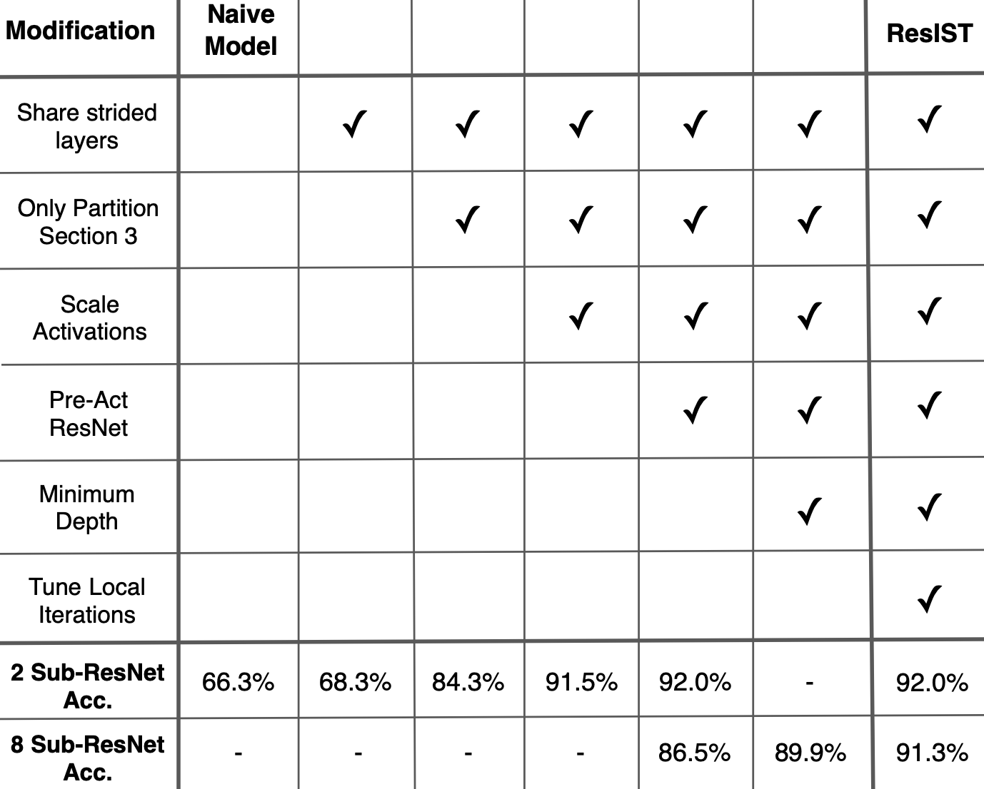
Extensive ablation experiments are conducted on the CIFAR10 dataset, outlined in Fig. 6, to empirically motivate the design choices made within ResIST (i.e., see Sec. 2.6). For the two sub-ResNet case, the naive implementation of ResIST, which evenly splits all convolutional blocks between subnetworks, is shown to perform poorly (i.e., $<$70% on CIFAR10). The accuracy of ResIST is improved over 25% by only allowing select layers to be partitioned and ensuring activations are scaled correctly when performing inference with the full network. The pre-activation ResNet is shown to yield an improvement in accuracy, leading ResIST to perform near optimally with two sub-ResNets.

Refer to caption
Figure 6: Test accuracies on the CIFAR10 dataset for a single run for the major ablation experiments performed with ResIST.

When ResIST is expanded to eight sub-ResNets, we initially observe a significant decrease in model accuracy. However, as can be seen in Fig. 6, this gap can be closed by enforcing a minimum depth on sub-ResNets and tuning the number of local iterations. By making these extra modifications, ResIST begins to perform similarly with two to eight sub-ResNets, yielding compelling performance.

A.2 Shallow Ensembles

The ResIST algorithm requires that independently-trained sub-ResNets must have their parameters synchronized intermittently. Such synchronization, however, can be completely avoided by training each sub-ResNet separately and forming an ensemble (i.e., ResIST without any aggregation). Although maintaining an ensemble has several drawbacks (e.g., slower inference, more parameters, etc.), the training time of the ensemble would nonetheless be reduced in comparison to ResIST by avoiding communication altogether. Therefore, the performance of such an ensemble should be compared to the models trained with ResIST.

Table 7: Performance of indpendently-trained ensembles of shallow ResNets in comparison to ResIST on CIFAR10 and CIFAR100 (denoted as C10 and C100, respectively).
Dataset Method 2 Model 4 Model 8 Model
C10 Ensemble 92.27 % $\pm$ 0.00 92.56% $\pm$ 0.03 90.67 % $\pm$ 0.04
ResIST 91.95% $\pm$ 0.32 92.35% $\pm$ 0.22 91.45% $\pm$ 0.30
C100 Ensemble 72.08% $\pm$ 0.05 72.12% $\pm$ 0.04 67.98 % $\pm$ 0.12
ResIST 70.06% $\pm$ 0.51 71.30% $\pm$ 0.20 70.26% $\pm$ 0.21
Table 8: Test accuracy on CIFAR10 (C10) and CIFAR100 (C100) for deeper architectures trained with ResIST and local SGD (LSGD). All tests were performed with 100 local iterations between synchronization rounds. All models were trained for 80 epochs.
ResNet152 ResNet200
Dataset # Machines Method Time Test Acc. Speedup Time Test Acc. Speedup
C10 2 LSGD 3512s 92.27% $\pm$ 0.003 4575s 92.31% $\pm$ 0.001
ResIST 2215s 92.01% $\pm$ 0.002 1.58$\times$ 2380s 92.10% $\pm$ 0.001 1.92$\times$
4 LSGD 3598s 91.39% $\pm$ 0.001 4357s 91.35% $\pm$ 0.000
ResIST 1054s 90.67% $\pm$ 0.001 3.41$\times$ 1161s 90.27% $\pm$ 0.001 3.75$\times$
C100 2 LSGD 3528s 70.50% $\pm$ 0.003 4639s 71.05% $\pm$ 0.005
ResIST 2291s 70.32% $\pm$ 0.005 1.53$\times$ 2202s 70.71% $\pm$ 0.002 2.10$\times$
4 LSGD 3518s 68.39% $\pm$ 0.004 4391s 69.05% $\pm$ 0.003
ResIST 1164s 67.27% $\pm$ 0.003 3.02$\times$ 1195s 67.62% $\pm$ 0.001 3.67$\times$

The performance of sub-ResNet ensembles in comparison to models trained with ResIST is displayed in Table 7. For 8 Sub-ResNets, the shallow ensembles achieve inferior performance in comparison to ResIST. When two and four Sub-ResNets are used, the performance of shallow ensembles and ResIST is comparable (i.e., $<1\%$ performance difference in most cases). However, it should be noted that such shallow ensembles of two or four sub-ResNets, in comparison to ResIST, cause a $2\times$ to $4\times$ slowdown in inference time (i.e., inference time for a single Sub-ResNet is not significantly faster than that of the global ResNet). Furthermore, the ensembles consume more parameters in comparison to global ResNet trained with ResIST.

A.3 Robustness to Local Iterations

Refer to caption
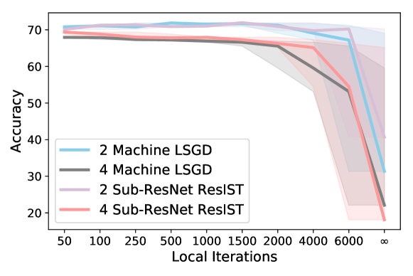
Figure 7: Test accuracy on CIFAR100 for ResNet-101 trained with both ResIST and local SGD (LSGD) with different numbers of local iterations. $\infty$ local iterations refers to aggregating parameters only once at the end of training (i.e., single-shot averaging). Shaded regions reflect deviations in accuracy.

ResIST is robust to various numbers of local iterations [Lin etย al., 2018, Zhang etย al., 2016, McMahan etย al., 2017]. An extensive sweep over possible values of $\ell$ is performed on CIFAR100. The results of this experiment are depicted in Fig. 7. As can be seen, ResIST achieves high accuracy even with thousands of local SGD iterations (i.e., previous work typically uses much fewer [Lin etย al., 2018]). However, if more sub-ResNets are used, performance tends to deteriorate more quickly as local iterations increase. Due to the robustness of ResIST to large numbers of local iterations, training can be accelerated without deteriorating model performance by simply increasing the value of $\ell$. Local SGD was found to demonstrate similar robustness to the number of local iterations, as shown in Fig. 7.

A.4 Deeper architectures

The ResIST methodology is easily applicable to deeper architectures. To demonstrate this, results are replicated for CIFAR10 and CIFAR100 datasets with ResNet152 and ResNet200. These deeper architectures are identical to the original ResNet101 architecture (i.e., see Fig. 2). However, more residual blocks are added to the third section of the ResNet (i.e., the highlighted portion of Fig. 2) to increase the modelโ€™s depth. It should be noted that convolutional blocks within the third section of the ResNet are partitioned in ResIST by default (see Sec. 2.2). As a result, all extra residual blocks within these deeper architectures are partitioned to sub-ResNets by ResIST (i.e., no extra blocks are shared between sub-ResNets), allowing ResIST to achieve greater acceleration in comparison to local SGD.

The results of experiments with deeper ResNets are presented in Table 8. ResIST performs competitively with localSGD in all cases. Furthermore, ResIST achieves a significant speedup in comparison to local SGD that becomes more pronounced as the model becomes deeper. E.g., for 4-GPUs, ResIST completes training $>3\times$ faster than local SGD for ResNet200 on both datasets. This speedup is caused by a greater ratio of total network blocks being partitioned to sub-ResNets in ResIST. While local SGD must communicate all parameters between machines, ResIST achieves a relative decrease in communication by partitioning all extra residual blocks evenly between sub-ResNets.

A.5 ResIST and Quantization/Sparse Gradients

Many quantization [Alistarh etย al., 2017, Yu etย al., 2019] and sparsification [Aji and Heafield, 2017, Jiang and Agrawal, 2018] techniques have been proposed for reducing communication costs in distributed training. Such techniques focus on compressing communicated data, and they do not interfere with our methodology, which provides a novel approach to model synchronization and training. The proposed approach can be easily combined with existing compression techniques to further reduce communication costs and accelerate training with no extra tuning or modifications. 
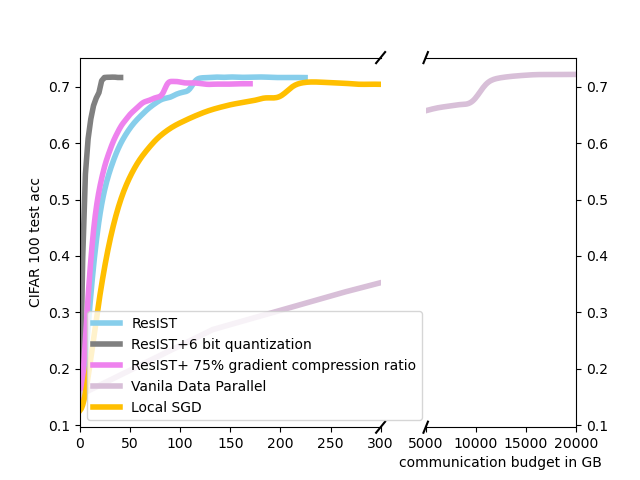
To demonstrate that ResIST works well with quantization, we compress all communicated parameters using both four-bit and eight-bit compression. Table 9 shows that ResIST retains its performance until the compression level reaches five-bit and lower. We also perform experiments with sparsification of communicated weights by only keeping 25% of total weights within each synchronization round. Such a strategy reaches a validation peformance of 71.25% on CIFAR100. We summarize the results of all quantization experiments in Fig. 8, where we compare communication budgets across different compression techniques with ResIST. From this figure, it is clear that ResIST is most efficient with six-bit quantization and is compatible with most main-stream compression techniques.

Table 9: Test Accuracy for ResIST combined with quantization on CIFAR10 and CIFAR100 (denoted as C10 and C100).
Dataset 8 bit 7 bit 6 bit 5 bit 4 bit
C10 92.14% 92.26% 91.91% 91.35% 76.33%
C100 71.38% 72.15% 71.37% 68.29% 40.48%
Refer to caption
Figure 8: Test accuracy vs. communication budget for ResIST, ResIST+quantization, ResIST+gradient compression, local SGD and vanilla data parallel on CIFAR100. All models are trained over a 4-GPU cluster.

Appendix B Proof for ResIST

Suppose we have $S$ workers, for subnetwork $v$ at local training step $l_{t}\leq\ell$ and global synchronization step $t\leq T$:

$\displaystyle\mathbf{x}^{(1)}_{v,l_{t},t}$ $\displaystyle=\sqrt{\frac{c_{\sigma}}{m}}\sigma\left(\mathbf{W}^{(1)}_{v,l_{t},t}\mathbf{x_{v,l_{t},t}}\right),$
$\displaystyle\mathbf{x}^{(h)}_{v,l_{t},t}$ =๐ฑv,lt,t(hโˆ’1)+crโ€‹eโ€‹sHโ€‹mโ€‹ฯƒโ€‹(๐–v,lt,t(h)โ€‹๐ฑv,lt,t(hโˆ’1))โ€‹Mv,t(h)absentsubscriptsuperscript๐ฑโ„Ž1๐‘ฃsubscript๐‘™๐‘ก๐‘กsubscript๐‘๐‘Ÿ๐‘’๐‘ ๐ป๐‘š๐œŽsubscriptsuperscript๐–โ„Ž๐‘ฃsubscript๐‘™๐‘ก๐‘กsubscriptsuperscript๐ฑโ„Ž1๐‘ฃsubscript๐‘™๐‘ก๐‘กsubscriptsuperscript๐‘€โ„Ž๐‘ฃ๐‘ก\displaystyle=\mathbf{x}^{(h-1)}_{v,l_{t},t}+\frac{c_{res}}{H\sqrt{m}}\sigma\left(\mathbf{W}^{(h)}_{v,l_{t},t}\mathbf{x}^{(h-1)}_{v,l_{t},t}\right)M^{(h)}_{v,t}
ย forย โ€‹2โ‰คhโ‰คH,ย forย 2โ„Ž๐ป\displaystyle\leavevmode\nobreak\ \leavevmode\nobreak\ \leavevmode\nobreak\ \leavevmode\nobreak\ \leavevmode\nobreak\ \leavevmode\nobreak\ \leavevmode\nobreak\ \leavevmode\nobreak\ \leavevmode\nobreak\ \leavevmode\nobreak\ \leavevmode\nobreak\ \leavevmode\nobreak\ \leavevmode\nobreak\ \leavevmode\nobreak\ \leavevmode\nobreak\ \leavevmode\nobreak\ \leavevmode\nobreak\ \leavevmode\nobreak\ \leavevmode\nobreak\ \leavevmode\nobreak\ \leavevmode\nobreak\ \leavevmode\nobreak\ \leavevmode\nobreak\ \leavevmode\nobreak\ \leavevmode\nobreak\ \leavevmode\nobreak\ \leavevmode\nobreak\ \leavevmode\nobreak\ \leavevmode\nobreak\ \leavevmode\nobreak\ \leavevmode\nobreak\ \text{ for }2\leq h\leq H,
frโ€‹eโ€‹sโ€‹(๐ฑ,ฮธ)subscript๐‘“๐‘Ÿ๐‘’๐‘ ๐ฑ๐œƒ\displaystyle f_{res}(\mathbf{x},\mathbf{\theta}) $\displaystyle=\mathbf{a}_{v,l_{t},t}^{\top}\mathbf{x}^{(H)}_{v,l_{t},t}$

where 0<crโ€‹eโ€‹s<10subscript๐‘๐‘Ÿ๐‘’๐‘ 10<c_{res}<1 is a small constant and $M^{(h)}_{v,t}$ is random binary variable in layer dropout or the indicator in ResIST that indicates whether this layer is partitioned to this subnetwork. such mask variable is constant during local training steps and re-sampled/re-assigned at global synchronization step. In ResIST and other research on layer dropout for ResNet, last layer is never dropped/paritioned but shared with all workers. Thus, in the following proof, we will follow this setting.

Note here we use a crโ€‹eโ€‹sHโ€‹msubscript๐‘๐‘Ÿ๐‘’๐‘ ๐ป๐‘š\frac{c_{res}}{H\sqrt{m}} scaling.

The gradient for subnetwork is

$\displaystyle\frac{\partial L}{\partial\mathbf{W}^{(h)}_{v,l_{t},t}}=$ crโ€‹eโ€‹sHโ€‹mโ€‹โˆ‘i=1n(yiโˆ’ui)โ€‹๐ฑi,v,lt,t(hโˆ’1)โ‹…[๐šv,lt,tโŠคโ€‹โˆl=h+1H(๐ˆ+crโ€‹eโ€‹sHโ€‹mโ€‹๐‰i,v,lt,t(l)โ€‹๐–v,lt,t(l)โ€‹Mv,t(l))โ€‹๐‰i,v,lt,t(h)โ€‹Mv,t(h)]subscript๐‘๐‘Ÿ๐‘’๐‘ ๐ป๐‘šsuperscriptsubscript๐‘–1๐‘›โ‹…subscript๐‘ฆ๐‘–subscript๐‘ข๐‘–superscriptsubscript๐ฑ๐‘–๐‘ฃsubscript๐‘™๐‘ก๐‘กโ„Ž1delimited-[]superscriptsubscript๐š๐‘ฃsubscript๐‘™๐‘ก๐‘กtopsuperscriptsubscriptproduct๐‘™โ„Ž1๐ป๐ˆsubscript๐‘๐‘Ÿ๐‘’๐‘ ๐ป๐‘šsuperscriptsubscript๐‰๐‘–๐‘ฃsubscript๐‘™๐‘ก๐‘ก๐‘™superscriptsubscript๐–๐‘ฃsubscript๐‘™๐‘ก๐‘ก๐‘™subscriptsuperscript๐‘€๐‘™๐‘ฃ๐‘กsuperscriptsubscript๐‰๐‘–๐‘ฃsubscript๐‘™๐‘ก๐‘กโ„Žsubscriptsuperscript๐‘€โ„Ž๐‘ฃ๐‘ก\displaystyle\frac{c_{res}}{H\sqrt{m}}\sum_{i=1}^{n}(y_{i}-u_{i})\mathbf{x}_{i,v,l_{t},t}^{(h-1)}\cdot\left[\mathbf{a}_{v,l_{t},t}^{\top}\prod_{l=h+1}^{H}\left(\mathbf{I}+\frac{c_{res}}{H\sqrt{m}}\mathbf{J}_{i,v,l_{t},t}^{(l)}\mathbf{W}_{v,l_{t},t}^{(l)}M^{(l)}_{v,t}\right)\mathbf{J}_{i,v,l_{t},t}^{(h)}M^{(h)}_{v,t}\right]

For subnetwork, $\mathbf{G}^{(H)}$ has the same form as in layer drop ResNet.

The accumulated gradients of all the subnetworks:

$\displaystyle\mathcal{W}^{(h)}_{t+1}-\mathcal{W}^{(h)}_{t}$ $\displaystyle=\eta\frac{\sum_{v=1}^{S}\sum_{l_{t}=1}^{\ell}\frac{\partial L}{\partial\mathbf{W}^{(h)}_{v,l_{t},t}}}{\sum_{v=1}^{S}M^{(h)}_{v,t}}$
=ฮทโˆ‘v=1SMv,t(h)โ€‹โˆ‘v=1Sโˆ‘lt=1โ„“crโ€‹eโ€‹sHโ€‹mโ€‹โˆ‘i=1n(yiโˆ’ui)โ€‹๐ฑi,v,lt,t(hโˆ’1)โ‹…[๐šv,lt,tโŠคโ€‹โˆl=h+1H(๐ˆ+crโ€‹eโ€‹sHโ€‹mโ€‹๐‰i,v,lt,t(l)โ€‹๐–v,lt,t(l)โ€‹Mv,t(l))โ€‹๐‰i,v,lt,t(h)โ€‹Mv,t(h)]absent๐œ‚superscriptsubscript๐‘ฃ1๐‘†subscriptsuperscript๐‘€โ„Ž๐‘ฃ๐‘กsuperscriptsubscript๐‘ฃ1๐‘†superscriptsubscriptsubscript๐‘™๐‘ก1โ„“subscript๐‘๐‘Ÿ๐‘’๐‘ ๐ป๐‘šsuperscriptsubscript๐‘–1๐‘›โ‹…subscript๐‘ฆ๐‘–subscript๐‘ข๐‘–superscriptsubscript๐ฑ๐‘–๐‘ฃsubscript๐‘™๐‘ก๐‘กโ„Ž1delimited-[]superscriptsubscript๐š๐‘ฃsubscript๐‘™๐‘ก๐‘กtopsuperscriptsubscriptproduct๐‘™โ„Ž1๐ป๐ˆsubscript๐‘๐‘Ÿ๐‘’๐‘ ๐ป๐‘šsuperscriptsubscript๐‰๐‘–๐‘ฃsubscript๐‘™๐‘ก๐‘ก๐‘™superscriptsubscript๐–๐‘ฃsubscript๐‘™๐‘ก๐‘ก๐‘™subscriptsuperscript๐‘€๐‘™๐‘ฃ๐‘กsuperscriptsubscript๐‰๐‘–๐‘ฃsubscript๐‘™๐‘ก๐‘กโ„Žsubscriptsuperscript๐‘€โ„Ž๐‘ฃ๐‘ก\displaystyle=\frac{\eta}{\sum_{v=1}^{S}M^{(h)}_{v,t}}\sum_{v=1}^{S}\sum_{l_{t}=1}^{\ell}\frac{c_{res}}{H\sqrt{m}}\sum_{i=1}^{n}(y_{i}-u_{i})\mathbf{x}_{i,v,l_{t},t}^{(h-1)}\cdot\left[\mathbf{a}_{v,l_{t},t}^{\top}\prod_{l=h+1}^{H}\left(\mathbf{I}+\frac{c_{res}}{H\sqrt{m}}\mathbf{J}_{i,v,l_{t},t}^{(l)}\mathbf{W}_{v,l_{t},t}^{(l)}M^{(l)}_{v,t}\right)\mathbf{J}_{i,v,l_{t},t}^{(h)}M^{(h)}_{v,t}\right]

The whole network at global synchronization step t+1

$\displaystyle\mathbf{x}^{(1)}_{t}$ $\displaystyle=\sqrt{\frac{c_{\sigma}}{m}}\sigma\left(\frac{\sum_{v=1}^{S}\mathbf{W}^{(1)}_{v,\ell,t}}{S}\mathbf{x_{t}}\right),$
$\displaystyle\mathbf{x}^{(h)}_{t}$ =๐ฑt(hโˆ’1)+crโ€‹eโ€‹sHโ€‹mโ€‹ฯƒโ€‹(โˆ‘v=1S๐–v,โ„“,t(h)โ€‹Mv,t(h)โˆ‘v=1SMv,t(h)โ€‹๐ฑt(hโˆ’1))absentsubscriptsuperscript๐ฑโ„Ž1๐‘กsubscript๐‘๐‘Ÿ๐‘’๐‘ ๐ป๐‘š๐œŽsuperscriptsubscript๐‘ฃ1๐‘†subscriptsuperscript๐–โ„Ž๐‘ฃโ„“๐‘กsubscriptsuperscript๐‘€โ„Ž๐‘ฃ๐‘กsuperscriptsubscript๐‘ฃ1๐‘†subscriptsuperscript๐‘€โ„Ž๐‘ฃ๐‘กsubscriptsuperscript๐ฑโ„Ž1๐‘ก\displaystyle=\mathbf{x}^{(h-1)}_{t}+\frac{c_{res}}{H\sqrt{m}}\sigma\left(\frac{\sum_{v=1}^{S}\mathbf{W}^{(h)}_{v,\ell,t}M^{(h)}_{v,t}}{\sum_{v=1}^{S}M^{(h)}_{v,t}}\mathbf{x}^{(h-1)}_{t}\right)
ย forย โ€‹2โ‰คhโ‰คH,ย forย 2โ„Ž๐ป\displaystyle\leavevmode\nobreak\ \leavevmode\nobreak\ \leavevmode\nobreak\ \leavevmode\nobreak\ \leavevmode\nobreak\ \leavevmode\nobreak\ \leavevmode\nobreak\ \leavevmode\nobreak\ \leavevmode\nobreak\ \leavevmode\nobreak\ \leavevmode\nobreak\ \leavevmode\nobreak\ \leavevmode\nobreak\ \leavevmode\nobreak\ \leavevmode\nobreak\ \leavevmode\nobreak\ \leavevmode\nobreak\ \leavevmode\nobreak\ \leavevmode\nobreak\ \leavevmode\nobreak\ \leavevmode\nobreak\ \leavevmode\nobreak\ \leavevmode\nobreak\ \leavevmode\nobreak\ \leavevmode\nobreak\ \leavevmode\nobreak\ \leavevmode\nobreak\ \leavevmode\nobreak\ \leavevmode\nobreak\ \leavevmode\nobreak\ \leavevmode\nobreak\ \text{ for }2\leq h\leq H,
frโ€‹eโ€‹sโ€‹(๐ฑ,ฮธ)subscript๐‘“๐‘Ÿ๐‘’๐‘ ๐ฑ๐œƒ\displaystyle f_{res}(\mathbf{x},\mathbf{\theta}) $\displaystyle=\frac{\sum_{v=1}^{S}\mathbf{a}_{v,\ell,t}}{S}^{\top}\mathbf{x}^{(H)}_{t}$

Let $\mathcal{W}^{(h)}_{t}=\frac{\sum_{v=1}^{S}\mathbf{W}^{(h)}_{v,\ell,t}M^{(h)}_{v,t}}{\sum_{v=1}^{S}M^{(h)}_{v,t}}$, $\mathbf{a}_{t}=\frac{\sum_{v=1}^{S}\mathbf{a}_{v,\ell,t}}{S}$

The whole network at global synchronization step 0

$\displaystyle\mathbf{x}^{(1)}_{0}$ $\displaystyle=\sqrt{\frac{c_{\sigma}}{m}}\sigma\left(\mathbf{W}^{(1)}_{0}\mathbf{x}\right),$
$\displaystyle\mathbf{x}^{(h)}_{0}$ =๐ฑ0(hโˆ’1)+crโ€‹eโ€‹sHโ€‹mโ€‹ฯƒโ€‹(๐–0(h)โ€‹๐ฑ0(hโˆ’1))absentsubscriptsuperscript๐ฑโ„Ž10subscript๐‘๐‘Ÿ๐‘’๐‘ ๐ป๐‘š๐œŽsubscriptsuperscript๐–โ„Ž0subscriptsuperscript๐ฑโ„Ž10\displaystyle=\mathbf{x}^{(h-1)}_{0}+\frac{c_{res}}{H\sqrt{m}}\sigma\left(\mathbf{W}^{(h)}_{0}\mathbf{x}^{(h-1)}_{0}\right)
ย forย โ€‹2โ‰คhโ‰คH,ย forย 2โ„Ž๐ป\displaystyle\leavevmode\nobreak\ \leavevmode\nobreak\ \leavevmode\nobreak\ \leavevmode\nobreak\ \leavevmode\nobreak\ \leavevmode\nobreak\ \leavevmode\nobreak\ \leavevmode\nobreak\ \leavevmode\nobreak\ \leavevmode\nobreak\ \leavevmode\nobreak\ \leavevmode\nobreak\ \leavevmode\nobreak\ \leavevmode\nobreak\ \leavevmode\nobreak\ \leavevmode\nobreak\ \leavevmode\nobreak\ \leavevmode\nobreak\ \leavevmode\nobreak\ \leavevmode\nobreak\ \leavevmode\nobreak\ \leavevmode\nobreak\ \leavevmode\nobreak\ \leavevmode\nobreak\ \leavevmode\nobreak\ \leavevmode\nobreak\ \leavevmode\nobreak\ \leavevmode\nobreak\ \leavevmode\nobreak\ \leavevmode\nobreak\ \leavevmode\nobreak\ \text{ for }2\leq h\leq H,
frโ€‹eโ€‹sโ€‹(๐ฑ,ฮธ)subscript๐‘“๐‘Ÿ๐‘’๐‘ ๐ฑ๐œƒ\displaystyle f_{res}(\mathbf{x},\mathbf{\theta}) $\displaystyle=\mathbf{a}_{0}^{\top}\mathbf{x}^{(H)}_{0}$

B.1 Proof Sketch

We can write the loss of the whole network at global syncrhonization step t+1 as

$$L(\mathbf{\theta}(t),\mathbf{M}_{1,t},\mathbf{M}_{2,t}...\mathbf{M}_{S,t})=\frac{1}{2}\left\|\mathbf{y}-\mathbf{u}(t,\mathbf{M}_{1,t},\mathbf{M}_{2,t}...\mathbf{M}_{S,t})\right\|_{2}^{2}.$$

where $\mathbf{M}_{v,t}=\{M^{(1)}_{v,t},M^{(2)}_{v,t}...M^{(H)}_{v,t}\}$ Let $\mathcal{M}_{t}=\{\mathbf{M}_{1,t},\mathbf{M}_{2,t}...\mathbf{M}_{S,t}\}$

For convience, we drop all mask notation in the following proof. Let $\hat{u}(t)$ be the output of the whole network at global synchronization step $t+1$. Now recall the progress of loss function:

$\displaystyle\left\|\mathbf{y}-\mathbf{\hat{u}}(t+1)\right\|_{2}^{2}=$ $\displaystyle\left\|\mathbf{y}-\mathbf{\hat{u}}(t)\right\|_{2}^{2}-2\left(\mathbf{y}-\mathbf{\hat{u}}(t)\right)^{\top}\left(\mathbf{\hat{u}}(t+1)-\mathbf{\hat{u}}(t)\right)+\left\|\mathbf{\hat{u}}(t+1)-\mathbf{\hat{u}}(t)\right\|_{2}^{2}$

Following Du etย al. [2019], we apply Taylor expansion on $\left(\mathbf{\hat{u}}(t+1)-\mathbf{\hat{u}}(t)\right)$ and look at the $i$th coordinate.

$\displaystyle\hat{u}_{i}(t+1)-\hat{u}_{i}(t)$ =โˆ’โŸจฮธโ€‹(t+1)โˆ’ฮธโ€‹(t),u^iโ€ฒโ€‹(ฮธโ€‹(t))โŸฉ+โˆซs=01โŸจฮธโ€‹(t+1)โˆ’ฮธโ€‹(t),u^iโ€ฒโ€‹(ฮธโ€‹(t))โˆ’u^iโ€ฒโ€‹(ฮธโ€‹(t)โˆ’sโ€‹(ฮธโ€‹(t)โˆ’ฮธโ€‹(t+1)))โŸฉโ€‹๐‘‘sabsent๐œƒ๐‘ก1๐œƒ๐‘กsubscriptsuperscript^๐‘ขโ€ฒ๐‘–๐œƒ๐‘กsuperscriptsubscript๐‘ 01๐œƒ๐‘ก1๐œƒ๐‘กsubscriptsuperscript^๐‘ขโ€ฒ๐‘–๐œƒ๐‘กsubscriptsuperscript^๐‘ขโ€ฒ๐‘–๐œƒ๐‘ก๐‘ ๐œƒ๐‘ก๐œƒ๐‘ก1differential-d๐‘ \displaystyle=-\langle\theta(t+1)-\theta(t),\hat{u}^{\prime}_{i}\left(\mathbf{\theta}(t)\right)\rangle+\int_{s=0}^{1}\langle\theta(t+1)-\theta(t),\hat{u}^{\prime}_{i}\left(\mathbf{\theta}(t)\right)-\hat{u}^{\prime}_{i}\left(\mathbf{\theta}(t)-s(\mathbf{\theta}(t)-\mathbf{\theta}(t+1))\right)\rangle ds
$\displaystyle\triangleq I^{i}_{1}(t)+I_{2}^{i}(t)$

However, it is not obvious that $I_{1}(t)$ and $I_{2}(t)$ can be directed bounded to show the decrease of the loss of the whole network as both of them involve the accumulated gradient change from distributed local subnetwork training. Thus, we introduce a new term $I^{\prime i}_{1}(t)$ as below, which relates to the hypothetical global gradient direction as if the whole network trained centrally.

$\displaystyle I^{\prime i}_{1}(t)=$ $\displaystyle-\eta\ell\langle L^{\prime}(\mathbf{\theta}(t)),\hat{u}^{\prime}_{i}\left(\mathbf{\theta}(t)\right)\rangle$
$\displaystyle=$ $\displaystyle-\eta\ell\sum_{j=1}^{n}(\hat{u}_{j}-y_{j})\langle\hat{u}^{\prime}_{j}(\mathbf{\theta}(t)),\hat{u}^{\prime}_{i}\left(\mathbf{\theta}(t)\right)\rangle$
$\displaystyle\triangleq$ $\displaystyle-\eta\ell\sum_{j=1}^{n}(\hat{u}_{j}-y_{j})\sum_{h=1}^{H+1}\mathbf{\hat{G}}^{(h)}_{ij}(t)$

Accordingly,

$\displaystyle\left\|\mathbf{y}-\mathbf{\hat{u}}(t+1)\right\|_{2}^{2}$
$\displaystyle=$ $\displaystyle\left\|\mathbf{y}-\mathbf{\hat{u}}(t)\right\|_{2}^{2}-2\left(\mathbf{y}-\mathbf{\hat{u}}(t)\right)^{\top}\left(\mathbf{I}_{1}(t)+\mathbf{I}_{2}(t)+\mathbf{I^{\prime}}_{1}(t)-\mathbf{I^{\prime}}_{1}(t)\right)+\left\|\mathbf{\hat{u}}(t+1)-\mathbf{\hat{u}}(t)\right\|_{2}^{2}$
$\displaystyle=$ $\displaystyle\left\|\mathbf{y}-\mathbf{\hat{u}}(t)\right\|_{2}^{2}-2\left(\mathbf{y}-\mathbf{\hat{u}}(t)\right)^{\top}\mathbf{I^{\prime}}_{1}(t)+2\left(\mathbf{y}-\mathbf{\hat{u}}(t)\right)^{\top}(\mathbf{I^{\prime}}_{1}(t)-\mathbf{I}_{1}(t))-2\left(\mathbf{y}-\mathbf{\hat{u}}(t)\right)^{\top}\mathbf{I}_{2}(t)+\left\|\mathbf{\hat{u}}(t+1)-\mathbf{\hat{u}}(t)\right\|_{2}^{2}$
$\displaystyle\leq$ $\displaystyle\left(1-\eta\ell\lambda_{\min}\left(\mathbf{\hat{G}}^{(H)}(t)\right)\right)\left\|\mathbf{y}-\mathbf{\hat{u}}(t)\right\|_{2}^{2}+2\left(\mathbf{y}-\mathbf{\hat{u}}(t)\right)^{\top}(\mathbf{I^{\prime}}_{1}(t)-\mathbf{I}_{1}(t))$
$\displaystyle-2\left(\mathbf{y}-\mathbf{\hat{u}}(t)\right)^{\top}\mathbf{I}_{2}(t)+\left\|\mathbf{\hat{u}}(t+1)-\mathbf{\hat{u}}(t)\right\|_{2}^{2}.$

Our hypothesis is:

Condition B.1.

At the $t+1$-th global synchronization, for the whole network, we have

$\displaystyle\left\|\mathbf{y}-\mathbf{\hat{u}}(t,\mathcal{M}_{t})\right\|_{2}^{2}\leq(1-\frac{\eta\ell\lambda_{0}}{2})^{t}\left\|\mathbf{y}-\mathbf{\hat{u}}(0)\right\|_{2}^{2}.$

In order to prove this, we need to show $2\left(\mathbf{y}-\mathbf{\hat{u}}(t)\right)^{\top}(\mathbf{I^{\prime}}_{1}(t)-\mathbf{I}_{1}(t))$,$-2\left(\mathbf{y}-\mathbf{\hat{u}}(t)\right)^{\top}\mathbf{I}_{2}(t)$ and $\left\|\mathbf{\hat{u}}(t+1)-\mathbf{\hat{u}}(t)\right\|_{2}^{2}$ are proportional to $\eta^{2}\left\|\mathbf{y}-\mathbf{\hat{u}}(t)\right\|_{2}^{2}$ so if we set $\eta$ sufficiently small, this term is smaller than $\eta\lambda_{\min}\left(\mathbf{\hat{G}}^{(H)}(t)\right)\left\|\mathbf{y}-\mathbf{\hat{u}}(t)\right\|_{2}^{2}$ and thus the loss function decreases with a linear rate.

Further, similar to Du etย al. [2019], to prove the induction hypothesis, it suffices to prove $\lambda_{\min}\left(\mathbf{\hat{G}}^{(H)}(t)\right)\geq\frac{\lambda_{0}}{2}$ for $t^{\prime}=0,\ldots,t$, where $\lambda_{0}$ is independent of $m$. Similar to Du etย al. [2019], we can show at the beginning

$\displaystyle\lambda_{\min}\left(\mathbf{\hat{G}}^{(H)}(0)\right)\geq\frac{3}{4}\lambda_{0}.$

Now for the $t$-th global iteration, by matrix perturbation analysis, we know it is sufficient to show $\left\|\mathbf{\hat{G}}^{(H)}(t)-\mathbf{\hat{G}}^{(H)}(0)\right\|_{2}\leq\frac{1}{4}\lambda_{0}$. To do this, we show as long as $m$ is large enough, every weight matrix is close its initialization in a relative error sense.

Lemma B.1 (Lemma on Initialization Norms for the whole network).

If $\sigma(\cdot)$ is $L-$Lipschitz and $m=\Omega\left(\frac{n}{\delta}\right)$, assuming $\left\|\mathcal{W}^{(h)}_{0}\right\|_{2}\leq c_{w,0}\sqrt{m}$ for $h\in[2,H]$ and $c_{w,0}\approx 2$ for Gaussian initialization. We have with probability at least $1-\delta$ over random initialization, for every $h\in[H]$ and $i\in[n]$,

$$\frac{1}{c_{x,0}}\leq\left\|\mathbf{x}_{i,0}^{(h)}\right\|_{2}\leq c_{x,0}$$

for some universal constant $c_{x,0}>1$

Proof of Lemmaย B.1.

As the global model at initialization is the same with original ResNet in Du etย al. [2019], we can use the same proof in Lemma C.1 in Du etย al. [2019]. โˆŽ

The following lemma lower bounds $\mathbf{\hat{G}}^{(H)}(0)$โ€™s least eigenvalue.

Lemma B.2 (Least Eigenvalue at the Initialization).

If $m=\Omega\left(\frac{n^{2}\log(Hn/\delta)}{\lambda_{0}^{2}}\right)$, we have

$\displaystyle\lambda_{\min}(\mathbf{\hat{G}}^{(H)}(0))\geq\frac{3}{4}\lambda_{0}.$
Proof of Lemmaย B.2.

As the global model at initialization is the same with original ResNet in Du etย al. [2019], we can use the same proof in Lemma C.2 in Du etย al. [2019]. โˆŽ

Lemma B.3.

Suppose $\sigma(\cdot)$ is $L$-Lipschitz and for $h\in[H]$, $\left\|\mathcal{W}^{(h)}_{0}\right\|_{2}\leq c_{w,0}\sqrt{m}$, $\left\|\mathbf{x}^{(h)}_{0}\right\|_{2}\leq c_{x,0}$ and $\left\|\mathbf{W}^{(h)}_{v,l_{t},t}-\mathcal{W}^{(h)}_{0}\right\|_{F}\leq\sqrt{m}R$ for some constant $c_{w,0},c_{x,0}>0$ and $R\leq c_{w,0}$ . Then we have

โ€–๐ฑv,lt,t(h)โˆ’๐ฑ0(h)โ€–2โ‰ค(cฯƒโ€‹L+cx,0cw,0+cx,0R)โ€‹e2โ€‹crโ€‹eโ€‹sโ€‹cw,0โ€‹Lโ€‹Rโ‰œcxโ€ฒโ€‹R.subscriptnormsubscriptsuperscript๐ฑโ„Ž๐‘ฃsubscript๐‘™๐‘ก๐‘กsubscriptsuperscript๐ฑโ„Ž02subscript๐‘๐œŽ๐ฟsubscript๐‘๐‘ฅ0subscript๐‘๐‘ค0subscript๐‘๐‘ฅ0๐‘…superscript๐‘’2subscript๐‘๐‘Ÿ๐‘’๐‘ subscript๐‘๐‘ค0๐ฟ๐‘…โ‰œsubscriptsuperscript๐‘โ€ฒ๐‘ฅ๐‘…\displaystyle\left\|\mathbf{x}^{(h)}_{v,l_{t},t}-\mathbf{x}^{(h)}_{0}\right\|_{2}\leq\left(\sqrt{c_{\sigma}}L+\frac{c_{x,0}}{c_{w,0}}+\frac{c_{x,0}}{R}\right)e^{2c_{res}c_{w,0}L}R\triangleq c^{\prime}_{x}R.
Proof of Lemmaย B.3.

We prove this lemma by induction. Our induction hypothesis is

$\displaystyle\left\|\mathbf{x}^{(h)}_{v,l_{t},t}-\mathbf{x}^{(h)}_{0}\right\|_{2}\leq g(h),$

where

gโ€‹(h)=[1+2โ€‹crโ€‹eโ€‹sโ€‹cw,0โ€‹LH]โ€‹gโ€‹(hโˆ’1)+crโ€‹eโ€‹sโ€‹Lโ€‹cx,0Hโ€‹(cw,0+R).๐‘”โ„Ždelimited-[]12subscript๐‘๐‘Ÿ๐‘’๐‘ subscript๐‘๐‘ค0๐ฟ๐ป๐‘”โ„Ž1subscript๐‘๐‘Ÿ๐‘’๐‘ ๐ฟsubscript๐‘๐‘ฅ0๐ปsubscript๐‘๐‘ค0๐‘…\displaystyle g(h)=\left[1+\frac{2c_{res}c_{w,0}L}{H}\right]g(h-1)+\frac{c_{res}Lc_{x,0}}{H}(c_{w,0}+R).

For $h=1$, we have

$\displaystyle\left\|\mathbf{x}^{(1)}_{v,l_{t},t}-\mathbf{x}^{(1)}_{0}\right\|_{2}$ $\displaystyle\leq\sqrt{\frac{c_{\sigma}}{m}}\left\|\sigma\left(\mathbf{W}^{(1)}_{v,l_{t},t}\mathbf{x}\right)-\sigma\left(\mathcal{W}^{(1)}_{0}\mathbf{x}\right)\right\|_{2}$
$\displaystyle\leq\sqrt{\frac{c_{\sigma}}{m}}L\left\|\mathbf{W}^{(1)}_{v,l_{t},t}-\mathcal{W}^{(1)}_{0}\right\|_{F}\leq\sqrt{c_{\sigma}}LR,$

which implies $g(1)=\sqrt{c_{\sigma}}LR$, for $2\leq h\leq H$, we have

โ€–๐ฑv,lt,t(h)โˆ’๐ฑ0(h)โ€–2โ‰คcrโ€‹eโ€‹sHโ€‹mโ€‹โ€–ฯƒโ€‹(๐–v,lt,t(h)โ€‹๐ฑv,lt,t(hโˆ’1))โ€‹Mv,t(h)โˆ’ฯƒโ€‹(๐’ฒ0(h)โ€‹๐ฑ0(hโˆ’1))โ€‹1โ€–2subscriptnormsubscriptsuperscript๐ฑโ„Ž๐‘ฃsubscript๐‘™๐‘ก๐‘กsubscriptsuperscript๐ฑโ„Ž02subscript๐‘๐‘Ÿ๐‘’๐‘ ๐ป๐‘šsubscriptnorm๐œŽsubscriptsuperscript๐–โ„Ž๐‘ฃsubscript๐‘™๐‘ก๐‘กsubscriptsuperscript๐ฑโ„Ž1๐‘ฃsubscript๐‘™๐‘ก๐‘กsubscriptsuperscript๐‘€โ„Ž๐‘ฃ๐‘ก๐œŽsubscriptsuperscript๐’ฒโ„Ž0subscriptsuperscript๐ฑโ„Ž1012\displaystyle\left\|\mathbf{x}^{(h)}_{v,l_{t},t}-\mathbf{x}^{(h)}_{0}\right\|_{2}\leq\frac{c_{res}}{H\sqrt{m}}\left\|\sigma\left(\mathbf{W}^{(h)}_{v,l_{t},t}\mathbf{x}^{(h-1)}_{v,l_{t},t}\right)M^{(h)}_{v,t}-\sigma\left(\mathcal{W}^{(h)}_{0}\mathbf{x}^{(h-1)}_{0}\right)1\right\|_{2}
$\displaystyle+\left\|\mathbf{x}^{(h-1)}_{v,l_{t},t}-\mathbf{x}^{(h-1)}_{0}\right\|_{2}$
โ‰คcrโ€‹eโ€‹sHโ€‹mโ€‹โ€–[ฯƒโ€‹(๐–v,lt,t(h)โ€‹๐ฑv,lt,t(hโˆ’1))โˆ’ฯƒโ€‹(๐’ฒ0(h)โ€‹๐ฑ0(hโˆ’1))]โ€‹Mv,t(h)+ฯƒโ€‹(๐’ฒ0(h)โ€‹๐ฑ0(hโˆ’1))โ€‹(Mv,t(h)โˆ’1)โ€–2absentsubscript๐‘๐‘Ÿ๐‘’๐‘ ๐ป๐‘šsubscriptnormdelimited-[]๐œŽsubscriptsuperscript๐–โ„Ž๐‘ฃsubscript๐‘™๐‘ก๐‘กsubscriptsuperscript๐ฑโ„Ž1๐‘ฃsubscript๐‘™๐‘ก๐‘ก๐œŽsubscriptsuperscript๐’ฒโ„Ž0subscriptsuperscript๐ฑโ„Ž10subscriptsuperscript๐‘€โ„Ž๐‘ฃ๐‘ก๐œŽsubscriptsuperscript๐’ฒโ„Ž0subscriptsuperscript๐ฑโ„Ž10subscriptsuperscript๐‘€โ„Ž๐‘ฃ๐‘ก12\displaystyle\leq\frac{c_{res}}{H\sqrt{m}}\left\|[\sigma\left(\mathbf{W}^{(h)}_{v,l_{t},t}\mathbf{x}^{(h-1)}_{v,l_{t},t}\right)-\sigma\left(\mathcal{W}^{(h)}_{0}\mathbf{x}^{(h-1)}_{0}\right)]M^{(h)}_{v,t}+\sigma\left(\mathcal{W}^{(h)}_{0}\mathbf{x}^{(h-1)}_{0}\right)(M^{(h)}_{v,t}-1)\right\|_{2}
$\displaystyle+\left\|\mathbf{x}^{(h-1)}_{v,l_{t},t}-\mathbf{x}^{(h-1)}_{0}\right\|_{2}$
โ‰คcrโ€‹eโ€‹sHโ€‹mโ€‹โ€–[ฯƒโ€‹(๐–v,lt,t(h)โ€‹๐ฑv,lt,t(hโˆ’1))โˆ’ฯƒโ€‹(๐’ฒ0(h)โ€‹๐ฑ0(hโˆ’1))]โ€‹Mv,t(h)โ€–2+crโ€‹eโ€‹sHโ€‹mโ€‹โ€–ฯƒโ€‹(๐’ฒ0(h)โ€‹๐ฑ0(hโˆ’1))โ€‹(Mv,t(h)โˆ’1)โ€–2absentsubscript๐‘๐‘Ÿ๐‘’๐‘ ๐ป๐‘šsubscriptnormdelimited-[]๐œŽsubscriptsuperscript๐–โ„Ž๐‘ฃsubscript๐‘™๐‘ก๐‘กsubscriptsuperscript๐ฑโ„Ž1๐‘ฃsubscript๐‘™๐‘ก๐‘ก๐œŽsubscriptsuperscript๐’ฒโ„Ž0subscriptsuperscript๐ฑโ„Ž10subscriptsuperscript๐‘€โ„Ž๐‘ฃ๐‘ก2subscript๐‘๐‘Ÿ๐‘’๐‘ ๐ป๐‘šsubscriptnorm๐œŽsubscriptsuperscript๐’ฒโ„Ž0subscriptsuperscript๐ฑโ„Ž10subscriptsuperscript๐‘€โ„Ž๐‘ฃ๐‘ก12\displaystyle\leq\frac{c_{res}}{H\sqrt{m}}\left\|[\sigma\left(\mathbf{W}^{(h)}_{v,l_{t},t}\mathbf{x}^{(h-1)}_{v,l_{t},t}\right)-\sigma\left(\mathcal{W}^{(h)}_{0}\mathbf{x}^{(h-1)}_{0}\right)]M^{(h)}_{v,t}\right\|_{2}+\frac{c_{res}}{H\sqrt{m}}\left\|\sigma\left(\mathcal{W}^{(h)}_{0}\mathbf{x}^{(h-1)}_{0}\right)(M^{(h)}_{v,t}-1)\right\|_{2}
$\displaystyle+\left\|\mathbf{x}^{(h-1)}_{v,l_{t},t}-\mathbf{x}^{(h-1)}_{0}\right\|_{2}$
โ‰คcrโ€‹eโ€‹sHโ€‹mโ€‹โ€–[ฯƒโ€‹(๐–v,lt,t(h)โ€‹๐ฑv,lt,t(hโˆ’1))โˆ’ฯƒโ€‹(๐’ฒ0(h)โ€‹๐ฑ0(hโˆ’1))]โ€–2โ€‹โ€–Mv,t(h)โ€–2+crโ€‹eโ€‹sHโ€‹mโ€‹โ€–ฯƒโ€‹(๐’ฒ0(h)โ€‹๐ฑ0(hโˆ’1))โ€–2โ€‹โ€–(Mv,t(h)โˆ’1)โ€–2absentsubscript๐‘๐‘Ÿ๐‘’๐‘ ๐ป๐‘šsubscriptnormdelimited-[]๐œŽsubscriptsuperscript๐–โ„Ž๐‘ฃsubscript๐‘™๐‘ก๐‘กsubscriptsuperscript๐ฑโ„Ž1๐‘ฃsubscript๐‘™๐‘ก๐‘ก๐œŽsubscriptsuperscript๐’ฒโ„Ž0subscriptsuperscript๐ฑโ„Ž102subscriptnormsubscriptsuperscript๐‘€โ„Ž๐‘ฃ๐‘ก2subscript๐‘๐‘Ÿ๐‘’๐‘ ๐ป๐‘šsubscriptnorm๐œŽsubscriptsuperscript๐’ฒโ„Ž0subscriptsuperscript๐ฑโ„Ž102subscriptnormsubscriptsuperscript๐‘€โ„Ž๐‘ฃ๐‘ก12\displaystyle\leq\frac{c_{res}}{H\sqrt{m}}\left\|[\sigma\left(\mathbf{W}^{(h)}_{v,l_{t},t}\mathbf{x}^{(h-1)}_{v,l_{t},t}\right)-\sigma\left(\mathcal{W}^{(h)}_{0}\mathbf{x}^{(h-1)}_{0}\right)]\right\|_{2}\left\|M^{(h)}_{v,t}\right\|_{2}+\frac{c_{res}}{H\sqrt{m}}\left\|\sigma\left(\mathcal{W}^{(h)}_{0}\mathbf{x}^{(h-1)}_{0}\right)\right\|_{2}\left\|(M^{(h)}_{v,t}-1)\right\|_{2}
$\displaystyle+\left\|\mathbf{x}^{(h-1)}_{v,l_{t},t}-\mathbf{x}^{(h-1)}_{0}\right\|_{2}$
โ‰คcrโ€‹eโ€‹sHโ€‹mโ€‹โ€–[ฯƒโ€‹(๐–v,lt,t(h)โ€‹๐ฑv,lt,t(hโˆ’1))โˆ’ฯƒโ€‹(๐–v,lt,t(h)โ€‹๐ฑ0(hโˆ’1))+ฯƒโ€‹(๐–v,lt,t(h)โ€‹๐ฑv,lt,t(hโˆ’1))โˆ’ฯƒโ€‹(๐’ฒ0(h)โ€‹๐ฑ0(hโˆ’1))]โ€–2absentsubscript๐‘๐‘Ÿ๐‘’๐‘ ๐ป๐‘šsubscriptnormdelimited-[]๐œŽsubscriptsuperscript๐–โ„Ž๐‘ฃsubscript๐‘™๐‘ก๐‘กsubscriptsuperscript๐ฑโ„Ž1๐‘ฃsubscript๐‘™๐‘ก๐‘ก๐œŽsubscriptsuperscript๐–โ„Ž๐‘ฃsubscript๐‘™๐‘ก๐‘กsubscriptsuperscript๐ฑโ„Ž10๐œŽsubscriptsuperscript๐–โ„Ž๐‘ฃsubscript๐‘™๐‘ก๐‘กsubscriptsuperscript๐ฑโ„Ž1๐‘ฃsubscript๐‘™๐‘ก๐‘ก๐œŽsubscriptsuperscript๐’ฒโ„Ž0subscriptsuperscript๐ฑโ„Ž102\displaystyle\leq\frac{c_{res}}{H\sqrt{m}}\left\|[\sigma\left(\mathbf{W}^{(h)}_{v,l_{t},t}\mathbf{x}^{(h-1)}_{v,l_{t},t}\right)-\sigma\left(\mathbf{W}^{(h)}_{v,l_{t},t}\mathbf{x}^{(h-1)}_{0}\right)+\sigma\left(\mathbf{W}^{(h)}_{v,l_{t},t}\mathbf{x}^{(h-1)}_{v,l_{t},t}\right)-\sigma\left(\mathcal{W}^{(h)}_{0}\mathbf{x}^{(h-1)}_{0}\right)]\right\|_{2}
+crโ€‹eโ€‹sโ€‹LHโ€‹mโ€‹โ€–๐’ฒ0(h)โ€‹๐ฑ0(hโˆ’1)โ€–+โ€–๐ฑv,lt,t(hโˆ’1)โˆ’๐ฑ0(hโˆ’1)โ€–2subscript๐‘๐‘Ÿ๐‘’๐‘ ๐ฟ๐ป๐‘šnormsubscriptsuperscript๐’ฒโ„Ž0subscriptsuperscript๐ฑโ„Ž10subscriptnormsubscriptsuperscript๐ฑโ„Ž1๐‘ฃsubscript๐‘™๐‘ก๐‘กsubscriptsuperscript๐ฑโ„Ž102\displaystyle+\frac{c_{res}L}{H\sqrt{m}}\left\|\mathcal{W}^{(h)}_{0}\mathbf{x}^{(h-1)}_{0}\right\|+\left\|\mathbf{x}^{(h-1)}_{v,l_{t},t}-\mathbf{x}^{(h-1)}_{0}\right\|_{2}
โ‰คcrโ€‹eโ€‹sHโ€‹mโ€‹โ€–ฯƒโ€‹(๐–v,lt,t(h)โ€‹๐ฑv,lt,t(hโˆ’1))โˆ’ฯƒโ€‹(๐–v,lt,t(h)โ€‹๐ฑ0(hโˆ’1))โ€–2absentsubscript๐‘๐‘Ÿ๐‘’๐‘ ๐ป๐‘šsubscriptnorm๐œŽsubscriptsuperscript๐–โ„Ž๐‘ฃsubscript๐‘™๐‘ก๐‘กsubscriptsuperscript๐ฑโ„Ž1๐‘ฃsubscript๐‘™๐‘ก๐‘ก๐œŽsubscriptsuperscript๐–โ„Ž๐‘ฃsubscript๐‘™๐‘ก๐‘กsubscriptsuperscript๐ฑโ„Ž102\displaystyle\leq\frac{c_{res}}{H\sqrt{m}}\left\|\sigma\left(\mathbf{W}^{(h)}_{v,l_{t},t}\mathbf{x}^{(h-1)}_{v,l_{t},t}\right)-\sigma\left(\mathbf{W}^{(h)}_{v,l_{t},t}\mathbf{x}^{(h-1)}_{0}\right)\right\|_{2}
+crโ€‹eโ€‹sHโ€‹mโ€‹โ€–ฯƒโ€‹(๐–v,lt,t(h)โ€‹๐ฑ0(hโˆ’1))โˆ’ฯƒโ€‹(๐’ฒ0(h)โ€‹๐ฑ0(hโˆ’1))โ€–2subscript๐‘๐‘Ÿ๐‘’๐‘ ๐ป๐‘šsubscriptnorm๐œŽsubscriptsuperscript๐–โ„Ž๐‘ฃsubscript๐‘™๐‘ก๐‘กsubscriptsuperscript๐ฑโ„Ž10๐œŽsubscriptsuperscript๐’ฒโ„Ž0subscriptsuperscript๐ฑโ„Ž102\displaystyle+\frac{c_{res}}{H\sqrt{m}}\left\|\sigma\left(\mathbf{W}^{(h)}_{v,l_{t},t}\mathbf{x}^{(h-1)}_{0}\right)-\sigma\left(\mathcal{W}^{(h)}_{0}\mathbf{x}^{(h-1)}_{0}\right)\right\|_{2}
+โ€–๐ฑv,lt,t(hโˆ’1)โˆ’๐ฑ0(hโˆ’1)โ€–2+crโ€‹eโ€‹sโ€‹Lโ€‹cw,0โ€‹cx,0Hsubscriptnormsubscriptsuperscript๐ฑโ„Ž1๐‘ฃsubscript๐‘™๐‘ก๐‘กsubscriptsuperscript๐ฑโ„Ž102subscript๐‘๐‘Ÿ๐‘’๐‘ ๐ฟsubscript๐‘๐‘ค0subscript๐‘๐‘ฅ0๐ป\displaystyle+\left\|\mathbf{x}^{(h-1)}_{v,l_{t},t}-\mathbf{x}^{(h-1)}_{0}\right\|_{2}+\frac{c_{res}Lc_{w,0}c_{x,0}}{H}
โ‰คcrโ€‹eโ€‹sโ€‹LHโ€‹mโ€‹(โ€–๐’ฒ0(h)โ€–2+โ€–๐–v,lt,t(h)โˆ’๐’ฒ0(h)โ€–F)โ‹…โ€–๐ฑv,lt,t(hโˆ’1)โˆ’๐ฑ0(hโˆ’1)โ€–2absentโ‹…subscript๐‘๐‘Ÿ๐‘’๐‘ ๐ฟ๐ป๐‘šsubscriptnormsubscriptsuperscript๐’ฒโ„Ž02subscriptnormsubscriptsuperscript๐–โ„Ž๐‘ฃsubscript๐‘™๐‘ก๐‘กsubscriptsuperscript๐’ฒโ„Ž0๐นsubscriptnormsubscriptsuperscript๐ฑโ„Ž1๐‘ฃsubscript๐‘™๐‘ก๐‘กsubscriptsuperscript๐ฑโ„Ž102\displaystyle\leq\frac{c_{res}L}{H\sqrt{m}}\left(\left\|\mathcal{W}^{(h)}_{0}\right\|_{2}+\left\|\mathbf{W}^{(h)}_{v,l_{t},t}-\mathcal{W}^{(h)}_{0}\right\|_{F}\right)\cdot\left\|\mathbf{x}^{(h-1)}_{v,l_{t},t}-\mathbf{x}^{(h-1)}_{0}\right\|_{2}
+crโ€‹eโ€‹sโ€‹LHโ€‹mโ€‹โ€–๐–v,lt,t(h)โˆ’๐’ฒ0(h)โ€–Fโ€‹โ€–๐ฑ0(hโˆ’1)โ€–2+โ€–๐ฑv,lt,t(hโˆ’1)โˆ’๐ฑ0(hโˆ’1)โ€–2+crโ€‹eโ€‹sโ€‹Lโ€‹cw,0โ€‹cx,0Hsubscript๐‘๐‘Ÿ๐‘’๐‘ ๐ฟ๐ป๐‘šsubscriptnormsubscriptsuperscript๐–โ„Ž๐‘ฃsubscript๐‘™๐‘ก๐‘กsubscriptsuperscript๐’ฒโ„Ž0๐นsubscriptnormsubscriptsuperscript๐ฑโ„Ž102subscriptnormsubscriptsuperscript๐ฑโ„Ž1๐‘ฃsubscript๐‘™๐‘ก๐‘กsubscriptsuperscript๐ฑโ„Ž102subscript๐‘๐‘Ÿ๐‘’๐‘ ๐ฟsubscript๐‘๐‘ค0subscript๐‘๐‘ฅ0๐ป\displaystyle+\frac{c_{res}L}{H\sqrt{m}}\left\|\mathbf{W}^{(h)}_{v,l_{t},t}-\mathcal{W}^{(h)}_{0}\right\|_{F}\left\|\mathbf{x}^{(h-1)}_{0}\right\|_{2}+\left\|\mathbf{x}^{(h-1)}_{v,l_{t},t}-\mathbf{x}^{(h-1)}_{0}\right\|_{2}+\frac{c_{res}Lc_{w,0}c_{x,0}}{H}
โ‰ค[1+crโ€‹eโ€‹sโ€‹LHโ€‹mโ€‹(cw,0โ€‹m+Rโ€‹m)]โ€‹gโ€‹(hโˆ’1)+crโ€‹eโ€‹sโ€‹LHโ€‹mโ€‹mโ€‹Rโ€‹cx,0+crโ€‹eโ€‹sโ€‹Lโ€‹cw,0โ€‹cx,0Habsentdelimited-[]1subscript๐‘๐‘Ÿ๐‘’๐‘ ๐ฟ๐ป๐‘šsubscript๐‘๐‘ค0๐‘š๐‘…๐‘š๐‘”โ„Ž1subscript๐‘๐‘Ÿ๐‘’๐‘ ๐ฟ๐ป๐‘š๐‘š๐‘…subscript๐‘๐‘ฅ0subscript๐‘๐‘Ÿ๐‘’๐‘ ๐ฟsubscript๐‘๐‘ค0subscript๐‘๐‘ฅ0๐ป\displaystyle\leq\left[1+\frac{c_{res}L}{H\sqrt{m}}\left(c_{w,0}\sqrt{m}+R\sqrt{m}\right)\right]g(h-1)+\frac{c_{res}L}{H\sqrt{m}}\sqrt{m}Rc_{x,0}+\frac{c_{res}Lc_{w,0}c_{x,0}}{H}
โ‰ค(1+2โ€‹crโ€‹eโ€‹sโ€‹cw,0โ€‹LH)โ€‹gโ€‹(hโˆ’1)+crโ€‹eโ€‹sHโ€‹Lโ€‹cx,0โ€‹R+crโ€‹eโ€‹sโ€‹Lโ€‹cw,0โ€‹cx,0H.absent12subscript๐‘๐‘Ÿ๐‘’๐‘ subscript๐‘๐‘ค0๐ฟ๐ป๐‘”โ„Ž1subscript๐‘๐‘Ÿ๐‘’๐‘ ๐ป๐ฟsubscript๐‘๐‘ฅ0๐‘…subscript๐‘๐‘Ÿ๐‘’๐‘ ๐ฟsubscript๐‘๐‘ค0subscript๐‘๐‘ฅ0๐ป\displaystyle\leq\left(1+\frac{2c_{res}c_{w,0}L}{H}\right)g(h-1)+\frac{c_{res}}{H}Lc_{x,0}R+\frac{c_{res}Lc_{w,0}c_{x,0}}{H}.

Lastly, simple calculations show gโ€‹(h)โ‰ค(cฯƒโ€‹L+cx,0cw,0+cx,0R)โ€‹e2โ€‹crโ€‹eโ€‹sโ€‹cw,0โ€‹Lโ€‹R๐‘”โ„Žsubscript๐‘๐œŽ๐ฟsubscript๐‘๐‘ฅ0subscript๐‘๐‘ค0subscript๐‘๐‘ฅ0๐‘…superscript๐‘’2subscript๐‘๐‘Ÿ๐‘’๐‘ subscript๐‘๐‘ค0๐ฟ๐‘…g(h)\leq\left(\sqrt{c_{\sigma}}L+\frac{c_{x,0}}{c_{w,0}}+\frac{c_{x,0}}{R}\right)e^{2c_{res}c_{w,0}L}R.

โˆŽ

Lemma B.4.

Suppose $\sigma(\cdot)$ is $L$-Lipschitz and for $h\in[H]$, $\left\|\mathcal{W}^{(h)}_{0}\right\|_{2}\leq c_{w,0}\sqrt{m}$, $\left\|\mathbf{x}^{(h)}_{0}\right\|_{2}\leq c_{x,0}$ and $\left\|\mathcal{W}^{(h)}_{t}-\mathcal{W}^{(h)}_{0}\right\|_{F}\leq\sqrt{m}R$ for some constant $c_{w,0},c_{x,0}>0$ and $R\leq c_{w,0}$ . Then we have

โ€–๐ฑt(h)โˆ’๐ฑ0(h)โ€–2โ‰ค(cฯƒโ€‹L+cx,0cw,0)โ€‹e2โ€‹crโ€‹eโ€‹sโ€‹cw,0โ€‹Lโ€‹Rโ‰œcxโ€‹R.subscriptnormsubscriptsuperscript๐ฑโ„Ž๐‘กsubscriptsuperscript๐ฑโ„Ž02subscript๐‘๐œŽ๐ฟsubscript๐‘๐‘ฅ0subscript๐‘๐‘ค0superscript๐‘’2subscript๐‘๐‘Ÿ๐‘’๐‘ subscript๐‘๐‘ค0๐ฟ๐‘…โ‰œsubscript๐‘๐‘ฅ๐‘…\displaystyle\left\|\mathbf{x}^{(h)}_{t}-\mathbf{x}^{(h)}_{0}\right\|_{2}\leq\left(\sqrt{c_{\sigma}}L+\frac{c_{x,0}}{c_{w,0}}\right)e^{2c_{res}c_{w,0}L}R\triangleq c_{x}R.
Proof of Lemmaย B.4.

The proof is exactly the same with proof of C.3 in Du etย al. [2019] โˆŽ

Next, we characterize how the perturbation on the weight matrices affect $\mathbf{\hat{G}}^{(H)}$.

Lemma B.5.

Suppose $\sigma(\cdot)$ is differentiable, $L-$Lipschitz and $\beta-$smooth. Suppose $\sigma(\cdot)$ is $L-$Lipschitz and $\beta-$smooth. Suppose for $h\in[H]$, $\left\|\mathcal{W}^{(h)}_{0}\right\|_{2}\leq c_{w,0}\sqrt{m}$, $\left\|\mathbf{a}_{0}\right\|_{2}\leq a_{2,0}\sqrt{m}$, $\left\|\mathbf{a}_{0}\right\|_{4}\leq a_{4,0}m^{1/4}$ , $\frac{1}{c_{x,0}}\leq\left\|\mathbf{x}^{(h)}_{0}\right\|_{2}\leq c_{x,0}$, if $\left\|\mathcal{W}^{(h)}_{r}-\mathcal{W}^{(h)}_{0}\right\|_{F},\left\|\mathbf{a}_{r}-\mathbf{a}_{0}\right\|_{2}\leq\sqrt{m}R$ where $R\leq c\lambda_{0}H^{2}n^{-1}$ and $R\leq c$ for some small constant $c$ , we have

$\displaystyle\left\|\mathbf{\hat{G}}^{(H)}(t)-\mathbf{\hat{G}}^{(H)}(0)\right\|_{2}\leq\frac{\lambda_{0}}{2}.$
Proof of Lemmaย B.5.

Similar to C.4 in Du etย al. [2019] Because Frobenius-norm of a matrix is bigger than the operator norm, it is sufficient to bound $\left\|\mathbf{\hat{G}}^{(H)}(t)-\mathbf{\hat{G}}^{(H)}(0)\right\|_{F}$. For simplicity define $z_{i,q}(t)=\mathcal{W}_{t,q}^{{(H)}\top}\mathbf{x}_{i,t}^{(H-1)}$, we have

$\displaystyle\left|\mathbf{\hat{G}}_{i,j}^{(H)}(t)-\mathbf{\hat{G}}_{i,j}^{(H)}(0)\right|$
$\displaystyle=$ crโ€‹eโ€‹s2H2โ€‹m|๐ฑi,t(Hโˆ’1)โŠคโ€‹๐ฑj,t(Hโˆ’1)โ€‹โˆ‘q=1maqโ€‹(t)2โ€‹ฯƒโ€ฒโ€‹(zi,qโ€‹(t))โ€‹ฯƒโ€ฒโ€‹(zj,qโ€‹(t))conditionalsuperscriptsubscript๐‘๐‘Ÿ๐‘’๐‘ 2superscript๐ป2๐‘šsuperscriptsubscript๐ฑ๐‘–๐‘กlimit-from๐ป1topsuperscriptsubscript๐ฑ๐‘—๐‘ก๐ป1superscriptsubscript๐‘ž1๐‘šsubscript๐‘Ž๐‘žsuperscript๐‘ก2superscript๐œŽโ€ฒsubscript๐‘ง๐‘–๐‘ž๐‘กsuperscript๐œŽโ€ฒsubscript๐‘ง๐‘—๐‘ž๐‘ก\displaystyle\frac{c_{res}^{2}}{H^{2}m}\big{|}\mathbf{x}_{i,t}^{(H-1)\top}\mathbf{x}_{j,t}^{(H-1)}\sum_{q=1}^{m}a_{q}(t)^{2}\sigma^{\prime}\left(z_{i,q}(t)\right)\sigma^{\prime}\left(z_{j,q}(t)\right)
$\displaystyle-\mathbf{x}_{i,0}^{(H-1)\top}\mathbf{x}_{j,0}^{(H-1)}\sum_{q=1}^{m}a_{q}(0)^{2}\sigma^{\prime}\left(z_{i,q}(0)\right)\sigma^{\prime}\left(z_{j,q}(0)\right)\big{|}$
$\displaystyle\leq$ crโ€‹eโ€‹s2H2โ€‹L2โ€‹a2,02โ€‹|๐ฑi,t(Hโˆ’1)โŠคโ€‹๐ฑj,t(Hโˆ’1)โˆ’๐ฑi,0(Hโˆ’1)โŠคโ€‹๐ฑj,0(Hโˆ’1)|superscriptsubscript๐‘๐‘Ÿ๐‘’๐‘ 2superscript๐ป2superscript๐ฟ2superscriptsubscript๐‘Ž202superscriptsubscript๐ฑ๐‘–๐‘กlimit-from๐ป1topsuperscriptsubscript๐ฑ๐‘—๐‘ก๐ป1superscriptsubscript๐ฑ๐‘–0limit-from๐ป1topsuperscriptsubscript๐ฑ๐‘—0๐ป1\displaystyle\frac{c_{res}^{2}}{H^{2}}L^{2}a_{2,0}^{2}\left|\mathbf{x}_{i,t}^{(H-1)\top}\mathbf{x}_{j,t}^{(H-1)}-\mathbf{x}_{i,0}^{(H-1)\top}\mathbf{x}_{j,0}^{(H-1)}\right|
+crโ€‹eโ€‹s2H2โ€‹cx,02mโ€‹|โˆ‘q=1maqโ€‹(0)2โ€‹(ฯƒโ€ฒโ€‹(zi,qโ€‹(t))โ€‹ฯƒโ€ฒโ€‹(zj,qโ€‹(t))โˆ’ฯƒโ€ฒโ€‹(zi,qโ€‹(0))โ€‹ฯƒโ€ฒโ€‹(zj,qโ€‹(0)))|superscriptsubscript๐‘๐‘Ÿ๐‘’๐‘ 2superscript๐ป2superscriptsubscript๐‘๐‘ฅ02๐‘šsuperscriptsubscript๐‘ž1๐‘šsubscript๐‘Ž๐‘žsuperscript02superscript๐œŽโ€ฒsubscript๐‘ง๐‘–๐‘ž๐‘กsuperscript๐œŽโ€ฒsubscript๐‘ง๐‘—๐‘ž๐‘กsuperscript๐œŽโ€ฒsubscript๐‘ง๐‘–๐‘ž0superscript๐œŽโ€ฒsubscript๐‘ง๐‘—๐‘ž0\displaystyle+\frac{c_{res}^{2}}{H^{2}}\frac{c_{x,0}^{2}}{m}\left|\sum_{q=1}^{m}a_{q}(0)^{2}\left(\sigma^{\prime}\left(z_{i,q}(t)\right)\sigma^{\prime}\left(z_{j,q}(t)\right)-\sigma^{\prime}\left(z_{i,q}(0)\right)\sigma^{\prime}\left(z_{j,q}(0)\right)\right)\right|
+crโ€‹eโ€‹s2H2โ€‹mโ€‹|๐ฑi,t(Hโˆ’1)โŠคโ€‹๐ฑj,t(Hโˆ’1)|โ€‹|โˆ‘q=1m(aqโ€‹(t)2โˆ’aqโ€‹(0)2)โ€‹ฯƒโ€ฒโ€‹(zi,qโ€‹(t))โ€‹ฯƒโ€ฒโ€‹(zj,qโ€‹(t))|superscriptsubscript๐‘๐‘Ÿ๐‘’๐‘ 2superscript๐ป2๐‘šsuperscriptsubscript๐ฑ๐‘–๐‘กlimit-from๐ป1topsuperscriptsubscript๐ฑ๐‘—๐‘ก๐ป1superscriptsubscript๐‘ž1๐‘šsubscript๐‘Ž๐‘žsuperscript๐‘ก2subscript๐‘Ž๐‘žsuperscript02superscript๐œŽโ€ฒsubscript๐‘ง๐‘–๐‘ž๐‘กsuperscript๐œŽโ€ฒsubscript๐‘ง๐‘—๐‘ž๐‘ก\displaystyle+\frac{c_{res}^{2}}{H^{2}m}\left|\mathbf{x}_{i,t}^{(H-1)\top}\mathbf{x}_{j,t}^{(H-1)}\right|\left|\sum_{q=1}^{m}\left(a_{q}(t)^{2}-a_{q}(0)^{2}\right)\sigma^{\prime}\left(z_{i,q}(t)\right)\sigma^{\prime}\left(z_{j,q}(t)\right)\right|
$\displaystyle\triangleq$ crโ€‹eโ€‹s2H2โ€‹(I1i,j+I2i,j+I3i,j).superscriptsubscript๐‘๐‘Ÿ๐‘’๐‘ 2superscript๐ป2superscriptsubscript๐ผ1๐‘–๐‘—superscriptsubscript๐ผ2๐‘–๐‘—superscriptsubscript๐ผ3๐‘–๐‘—\displaystyle\frac{c_{res}^{2}}{H^{2}}(I_{1}^{i,j}+I_{2}^{i,j}+I_{3}^{i,j}).

For $I_{1}^{i,j}$, using Lemmaย B.4, we have

$\displaystyle I_{1}^{i,j}=$ $\displaystyle L^{2}a_{2,0}^{2}\left|\mathbf{x}_{i,t}^{(H-1)\top}\mathbf{x}_{j,t}^{(H-1)}-\mathbf{x}_{i,0}^{(H-1)\top}\mathbf{x}_{j,0}^{(H-1)}\right|$
$\displaystyle\leq$ $\displaystyle L^{2}a_{2,0}^{2}\left|(\mathbf{x}_{i,t}^{(H-1)}-\mathbf{x}_{i,0}^{(H-1)}\top)\mathbf{x}_{j,t}^{(H-1)}\right|+L^{2}a_{2,0}^{2}\left|\mathbf{x}_{i,0}^{(H-1)\top}(\mathbf{x}_{i,t}^{(H-1)}-\mathbf{x}_{i,0}^{(H-1)})\right|$
$\displaystyle\leq$ $\displaystyle c_{x}L^{2}a_{2,0}^{2}R\cdot(c_{x,0}+c_{x}R)+c_{x,0}c_{x}L^{2}a_{2,0}^{2}R$
$\displaystyle\leq$ $\displaystyle 3c_{x,0}c_{x}L^{2}a_{2,0}^{2}R,$

Same with C.4 Du etย al. [2019], to bound $I_{2}^{i,j}$, we have

$\displaystyle I_{2}^{i,j}=$ $\displaystyle c_{x,0}^{2}\frac{1}{m}\left|\sum_{q=1}^{m}a_{q}(0)^{2}\sigma^{\prime}\left(z_{i,q}(t)\right)\sigma^{\prime}\left(z_{j,q}(t)\right)-a_{q}(0)^{2}\sigma^{\prime}\left(z_{i,q}(0)\right)\sigma^{\prime}\left(z_{j,q}(0)\right)\right|$
$\displaystyle\leq$ $\displaystyle\frac{\beta La_{4,0}^{2}c_{x,0}^{2}}{\sqrt{m}}\left(\sqrt{\sum_{q=1}^{m}\left|z_{i,q}(t)-z_{i,q}(0)\right|^{2}}+\sqrt{\sum_{q=1}^{m}\left|z_{j,q}(t)-z_{j,q}(0)\right|^{2}}\right).$

Using the same proof for Lemmaย B.4, it is easy to see

$\displaystyle\sum_{q=1}^{m}\left|z_{i,q}(t)-z_{i,q}(0)\right|^{2}\leq\left(2c_{x}c_{w,0}+c_{x,0}\right)^{2}L^{2}mR^{2}.$

Thus

$\displaystyle I_{2}^{i,j}\leq 2\beta c_{x,0}^{2}\left(2c_{x}c_{w,0}+c_{x,0}\right)L^{2}R.$

The bound of $I_{3}^{i,j}$ is the same to that $I_{3}^{i,j}$ in Du etย al. [2019] C.4,

$\displaystyle I_{3}^{i,j}$ $\displaystyle\leq 12L^{2}c_{x,0}^{2}a_{2,0}R.$

Therefore we can bound the perturbation

$\displaystyle\left\|\mathbf{\hat{G}}^{(H)}(t)-\mathbf{\hat{G}}^{(H)}(0)\right\|_{F}=$ $\displaystyle\sqrt{\sum_{(i,j)}^{{n,n}}\left|\mathbf{\hat{G}}_{i,j}^{(H)}(t)-\mathbf{\hat{G}}_{i,j}^{(H)}(0)\right|^{2}}$
$\displaystyle\leq\frac{c_{res}^{2}}{H^{2}}\sqrt{n^{2}(3c_{x,0}c_{x}L^{2}a_{2,0}^{2}R+2\beta c_{x,0}^{2}\left(2c_{x}c_{w,0}+c_{x,0}\right)L^{2}R+12L^{2}c_{x,0}^{2}a_{2,0}R})$
=crโ€‹eโ€‹s2H2โ€‹nโ€‹(3โ€‹cx,0โ€‹cxโ€‹L2โ€‹a2,02โ€‹R+2โ€‹ฮฒโ€‹cx,02โ€‹(2โ€‹cxโ€‹cw,0+cx,0)โ€‹L2โ€‹R+12โ€‹L2โ€‹cx,02โ€‹a2,0โ€‹R)absentsuperscriptsubscript๐‘๐‘Ÿ๐‘’๐‘ 2superscript๐ป2๐‘›3subscript๐‘๐‘ฅ0subscript๐‘๐‘ฅsuperscript๐ฟ2superscriptsubscript๐‘Ž202๐‘…2๐›ฝsuperscriptsubscript๐‘๐‘ฅ022subscript๐‘๐‘ฅsubscript๐‘๐‘ค0subscript๐‘๐‘ฅ0superscript๐ฟ2๐‘…12superscript๐ฟ2superscriptsubscript๐‘๐‘ฅ02subscript๐‘Ž20๐‘…\displaystyle=\frac{c_{res}^{2}}{H^{2}}n(3c_{x,0}c_{x}L^{2}a_{2,0}^{2}R+2\beta c_{x,0}^{2}\left(2c_{x}c_{w,0}+c_{x,0}\right)L^{2}R+12L^{2}c_{x,0}^{2}a_{2,0}R)
.

Plugging in the bound on $R$, we have the desired result. โˆŽ

Now we prove theorem 3.1 by induction, assume the condition B.1, we want to bound the change of weight to satisfy lemma B.5 and then we want to show $2\left(\mathbf{y}-\mathbf{\hat{u}}(t)\right)^{\top}(\mathbf{I^{\prime}}_{1}(t)-\mathbf{I}_{1}(t))$,$-2\left(\mathbf{y}-\mathbf{\hat{u}}(t)\right)^{\top}\mathbf{I}_{2}(t)$ and $\left\|\mathbf{\hat{u}}(t+1)-\mathbf{\hat{u}}(t)\right\|_{2}^{2}$ are proportional to $\eta^{2}\left\|\mathbf{y}-\mathbf{u}(t)\right\|_{2}^{2}$ so if we set $\eta$ sufficiently small, this term is smaller than $\eta\lambda_{\min}\left(\mathbf{\hat{G}}^{(H)}(t)\right)\left\|\mathbf{y}-\mathbf{u}(t)\right\|_{2}^{2}$ and thus the loss function decreases with a linear rate.

Lemma B.6.

If Conditionย B.1 holds for $t^{\prime}=0,\ldots,t-1$, we have for any $1\leq v\leq S$, $0\leq l_{t}\leq\ell$

$\displaystyle\left\|\mathbf{W}^{(h)}_{v,l_{t},t}-\mathcal{W}^{(h)}_{0}\right\|_{F},\left\|\mathbf{a}_{v,l_{t},t}-\mathbf{a}_{0}\right\|_{2}\leq R^{\prime}\sqrt{m},$
$\displaystyle\left\|\mathbf{W}^{(h)}_{v,l_{t},t}-\mathbf{W}^{(h)}_{v,l_{t}-1,t}\right\|_{F},\left\|\mathbf{a}_{v,l_{t},t}-\mathbf{a}_{v,l_{t}-1,t}\right\|_{2}\leq\eta Q^{\prime}(l_{t}-1,t),$

where Rโ€ฒ=16โ€‹crโ€‹eโ€‹sโ€‹cx,0โ€‹a2,0โ€‹Lโ€‹e2โ€‹crโ€‹eโ€‹sโ€‹cw,0โ€‹Lโ€‹nโ€‹โ€–๐ฒโˆ’๐ฎโ€‹(0)โ€–2Hโ€‹ฮป0โ€‹m<csuperscript๐‘…โ€ฒ16subscript๐‘๐‘Ÿ๐‘’๐‘ subscript๐‘๐‘ฅ0subscript๐‘Ž20๐ฟsuperscript๐‘’2subscript๐‘๐‘Ÿ๐‘’๐‘ subscript๐‘๐‘ค0๐ฟ๐‘›subscriptnorm๐ฒ๐ฎ02๐ปsubscript๐œ†0๐‘š๐‘R^{\prime}=\frac{16c_{res}c_{x,0}a_{2,0}Le^{2c_{res}c_{w,0}L}\sqrt{n}\left\|\mathbf{y}-\mathbf{u}(0)\right\|_{2}}{H\lambda_{0}\sqrt{m}}<c for some small constant $c$ ,
Qโ€ฒโ€‹(lt,t)=4โ€‹crโ€‹eโ€‹sโ€‹cx,0โ€‹a2,0โ€‹Lโ€‹e2โ€‹crโ€‹eโ€‹sโ€‹cw,0โ€‹Lโ€‹nโ€‹โ€–๐ฒโˆ’๐ฎt,ltโ€–2/Hsuperscript๐‘„โ€ฒsubscript๐‘™๐‘ก๐‘ก4subscript๐‘๐‘Ÿ๐‘’๐‘ subscript๐‘๐‘ฅ0subscript๐‘Ž20๐ฟsuperscript๐‘’2subscript๐‘๐‘Ÿ๐‘’๐‘ subscript๐‘๐‘ค0๐ฟ๐‘›subscriptnorm๐ฒsubscript๐ฎ๐‘กsubscript๐‘™๐‘ก2๐ปQ^{\prime}(l_{t},t)=4c_{res}c_{x,0}a_{2,0}Le^{2c_{res}c_{w,0}L}\sqrt{n}\left\|\mathbf{y}-\mathbf{u}_{t,l_{t}}\right\|_{2}/H and
Qโ€ฒโ€‹(t)=4โ€‹crโ€‹eโ€‹sโ€‹cx,0โ€‹a2,0โ€‹Lโ€‹e2โ€‹crโ€‹eโ€‹sโ€‹cw,0โ€‹Lโ€‹nโ€‹โ€–๐ฒโˆ’๐ฎ^tโ€–2/Hsuperscript๐‘„โ€ฒ๐‘ก4subscript๐‘๐‘Ÿ๐‘’๐‘ subscript๐‘๐‘ฅ0subscript๐‘Ž20๐ฟsuperscript๐‘’2subscript๐‘๐‘Ÿ๐‘’๐‘ subscript๐‘๐‘ค0๐ฟ๐‘›subscriptnorm๐ฒsubscript^๐ฎ๐‘ก2๐ปQ^{\prime}(t)=4c_{res}c_{x,0}a_{2,0}Le^{2c_{res}c_{w,0}L}\sqrt{n}\left\|\mathbf{y}-\mathbf{\hat{u}}_{t}\right\|_{2}/H.

Proof of Lemmaย B.6.

We will prove this corollary by induction. The induction hypothesis is

$\displaystyle\left\|\mathbf{W}^{(h)}_{v,l_{t},t}-\mathcal{W}^{(h)}_{0}\right\|_{F}$ $\displaystyle\leq R^{\prime}\sqrt{m}$
$\displaystyle\left\|\mathbf{a}_{v,l_{t},t}-\mathbf{a}_{0}\right\|_{2}$ $\displaystyle\leq R^{\prime}\sqrt{m}.$

First we want to prove it holds for $t^{\prime}=0$ and $0\leq l_{t}\leq\ell$.

We prove it by induction w.r.t $l_{t}$: It is easy to see that it holds for $t^{\prime}=0$ and $l_{t}^{\prime}=0$. Suppose it holds for $0\leq l_{t}^{\prime}\leq l_{t}$, we want to prove it holds for $l_{t}^{\prime}=l_{t}+1$ Following C.5 in Du etย al. [2019], note $\left\|\mathbf{J}_{i,v,l_{t},t}^{(k)}\right\|_{2}\leq L$. We have

$\displaystyle\left\|\mathbf{W}^{(h)}_{v,l_{t}+1,t}-\mathbf{W}^{(h)}_{v,l_{t},t}\right\|_{F}$
$\displaystyle\leq$ ฮทโ€‹crโ€‹eโ€‹sHโ€‹mโ€‹โ€–๐š๐ฏ,๐ฅ๐ญ,๐ญโ€–2โ€‹โˆ‘i=1n|yiโˆ’ui,v,lt,t|โ€‹โ€–๐ฑi,v,lt,t(hโˆ’1)โ€–2โ€‹โˆk=h+1Hโ€–๐ˆ+crโ€‹eโ€‹sHโ€‹mโ€‹๐‰i,v,lt,t(k)โ€‹๐–v,lt,t(k)โ€‹Mv,t(k)โ€–2โ€‹โ€–๐‰i,v,lt,t(k)โ€–2โ€‹โ€–Mv,t(h)โ€–2๐œ‚subscript๐‘๐‘Ÿ๐‘’๐‘ ๐ป๐‘šsubscriptnormsubscript๐š๐ฏsubscript๐ฅ๐ญ๐ญ2superscriptsubscript๐‘–1๐‘›subscript๐‘ฆ๐‘–subscript๐‘ข๐‘–๐‘ฃsubscript๐‘™๐‘ก๐‘กsubscriptnormsubscriptsuperscript๐ฑโ„Ž1๐‘–๐‘ฃsubscript๐‘™๐‘ก๐‘ก2superscriptsubscriptproduct๐‘˜โ„Ž1๐ปsubscriptnorm๐ˆsubscript๐‘๐‘Ÿ๐‘’๐‘ ๐ป๐‘šsuperscriptsubscript๐‰๐‘–๐‘ฃsubscript๐‘™๐‘ก๐‘ก๐‘˜subscriptsuperscript๐–๐‘˜๐‘ฃsubscript๐‘™๐‘ก๐‘กsuperscriptsubscript๐‘€๐‘ฃ๐‘ก๐‘˜2subscriptnormsuperscriptsubscript๐‰๐‘–๐‘ฃsubscript๐‘™๐‘ก๐‘ก๐‘˜2subscriptnormsuperscriptsubscript๐‘€๐‘ฃ๐‘กโ„Ž2\displaystyle\eta\frac{c_{res}}{H\sqrt{m}}\left\|\mathbf{a_{v,l_{t},t}}\right\|_{2}\sum_{i=1}^{n}\left|y_{i}-u_{i,v,l_{t},t}\right|\left\|\mathbf{x}^{(h-1)}_{i,v,l_{t},t}\right\|_{2}\prod_{k=h+1}^{H}\left\|\mathbf{I}+\frac{c_{res}}{H\sqrt{m}}\mathbf{J}_{i,v,l_{t},t}^{(k)}\mathbf{W}^{(k)}_{v,l_{t},t}M_{v,t}^{(k)}\right\|_{2}\left\|\mathbf{J}_{i,v,l_{t},t}^{(k)}\right\|_{2}\left\|M_{v,t}^{(h)}\right\|_{2}
$\displaystyle\leq$ ฮทโ€‹Lโ€‹crโ€‹eโ€‹sHโ€‹mโ€‹โ€–๐š๐ฏ,๐ฅ๐ญ,๐ญโ€–2โ€‹โˆ‘i=1n|yiโˆ’ui,v,lt,t|โ€‹โ€–๐ฑi,v,lt,t(hโˆ’1)โ€–2โ€‹โˆk=h+1Hโ€–๐ˆ+crโ€‹eโ€‹sHโ€‹mโ€‹๐‰i,v,lt,t(k)โ€‹๐–v,lt,t(k)โ€‹Mv,t(k)โ€–2๐œ‚๐ฟsubscript๐‘๐‘Ÿ๐‘’๐‘ ๐ป๐‘šsubscriptnormsubscript๐š๐ฏsubscript๐ฅ๐ญ๐ญ2superscriptsubscript๐‘–1๐‘›subscript๐‘ฆ๐‘–subscript๐‘ข๐‘–๐‘ฃsubscript๐‘™๐‘ก๐‘กsubscriptnormsubscriptsuperscript๐ฑโ„Ž1๐‘–๐‘ฃsubscript๐‘™๐‘ก๐‘ก2superscriptsubscriptproduct๐‘˜โ„Ž1๐ปsubscriptnorm๐ˆsubscript๐‘๐‘Ÿ๐‘’๐‘ ๐ป๐‘šsuperscriptsubscript๐‰๐‘–๐‘ฃsubscript๐‘™๐‘ก๐‘ก๐‘˜subscriptsuperscript๐–๐‘˜๐‘ฃsubscript๐‘™๐‘ก๐‘กsuperscriptsubscript๐‘€๐‘ฃ๐‘ก๐‘˜2\displaystyle\eta\frac{Lc_{res}}{H\sqrt{m}}\left\|\mathbf{a_{v,l_{t},t}}\right\|_{2}\sum_{i=1}^{n}\left|y_{i}-u_{i,v,l_{t},t}\right|\left\|\mathbf{x}^{(h-1)}_{i,v,l_{t},t}\right\|_{2}\prod_{k=h+1}^{H}\left\|\mathbf{I}+\frac{c_{res}}{H\sqrt{m}}\mathbf{J}_{i,v,l_{t},t}^{(k)}\mathbf{W}^{(k)}_{v,l_{t},t}M_{v,t}^{(k)}\right\|_{2}

Further

โˆk=h+1Hโ€–๐ˆ+crโ€‹eโ€‹sHโ€‹mโ€‹๐‰i,v,lt,t(k)โ€‹๐–v,lt,t(k)โ€‹Mv,t(k)โ€–2superscriptsubscriptproduct๐‘˜โ„Ž1๐ปsubscriptnorm๐ˆsubscript๐‘๐‘Ÿ๐‘’๐‘ ๐ป๐‘šsuperscriptsubscript๐‰๐‘–๐‘ฃsubscript๐‘™๐‘ก๐‘ก๐‘˜subscriptsuperscript๐–๐‘˜๐‘ฃsubscript๐‘™๐‘ก๐‘กsuperscriptsubscript๐‘€๐‘ฃ๐‘ก๐‘˜2\displaystyle\prod_{k=h+1}^{H}\left\|\mathbf{I}+\frac{c_{res}}{H\sqrt{m}}\mathbf{J}_{i,v,l_{t},t}^{(k)}\mathbf{W}^{(k)}_{v,l_{t},t}M_{v,t}^{(k)}\right\|_{2}
$\displaystyle\leq$ โˆk=h+1Hโ€–๐ˆโ€–2+โ€–crโ€‹eโ€‹sHโ€‹mโ€‹๐‰i,v,lt,t(k)โ€‹๐–v,lt,t(k)โ€‹Mv,t(k)โ€–2superscriptsubscriptproduct๐‘˜โ„Ž1๐ปsubscriptnorm๐ˆ2subscriptnormsubscript๐‘๐‘Ÿ๐‘’๐‘ ๐ป๐‘šsuperscriptsubscript๐‰๐‘–๐‘ฃsubscript๐‘™๐‘ก๐‘ก๐‘˜subscriptsuperscript๐–๐‘˜๐‘ฃsubscript๐‘™๐‘ก๐‘กsuperscriptsubscript๐‘€๐‘ฃ๐‘ก๐‘˜2\displaystyle\prod_{k=h+1}^{H}\left\|\mathbf{I}\right\|_{2}+\left\|\frac{c_{res}}{H\sqrt{m}}\mathbf{J}_{i,v,l_{t},t}^{(k)}\mathbf{W}^{(k)}_{v,l_{t},t}M_{v,t}^{(k)}\right\|_{2}
$\displaystyle\leq$ โˆk=h+1Hโ€–๐ˆโ€–2+crโ€‹eโ€‹sHโ€‹mโ€‹โ€–๐‰i,v,lt,t(k)โ€–2โ€‹โ€–๐–v,lt,t(k)โ€–2โ€‹โ€–Mv,t(k)โ€–2superscriptsubscriptproduct๐‘˜โ„Ž1๐ปsubscriptnorm๐ˆ2subscript๐‘๐‘Ÿ๐‘’๐‘ ๐ป๐‘šsubscriptnormsuperscriptsubscript๐‰๐‘–๐‘ฃsubscript๐‘™๐‘ก๐‘ก๐‘˜2subscriptnormsubscriptsuperscript๐–๐‘˜๐‘ฃsubscript๐‘™๐‘ก๐‘ก2subscriptnormsuperscriptsubscript๐‘€๐‘ฃ๐‘ก๐‘˜2\displaystyle\prod_{k=h+1}^{H}\left\|\mathbf{I}\right\|_{2}+\frac{c_{res}}{H\sqrt{m}}\left\|\mathbf{J}_{i,v,l_{t},t}^{(k)}\right\|_{2}\left\|\mathbf{W}^{(k)}_{v,l_{t},t}\right\|_{2}\left\|M_{v,t}^{(k)}\right\|_{2}
$\displaystyle\leq$ โˆk=h+1Hโ€–๐ˆโ€–2+crโ€‹eโ€‹sโ€‹LHโ€‹mโ€‹(โ€–๐’ฒ0(k)โ€–F+โ€–๐–v,lt,t(k)โˆ’๐’ฒ0(k)โ€–F)superscriptsubscriptproduct๐‘˜โ„Ž1๐ปsubscriptnorm๐ˆ2subscript๐‘๐‘Ÿ๐‘’๐‘ ๐ฟ๐ป๐‘šsubscriptnormsubscriptsuperscript๐’ฒ๐‘˜0๐นsubscriptnormsubscriptsuperscript๐–๐‘˜๐‘ฃsubscript๐‘™๐‘ก๐‘กsubscriptsuperscript๐’ฒ๐‘˜0๐น\displaystyle\prod_{k=h+1}^{H}\left\|\mathbf{I}\right\|_{2}+\frac{c_{res}L}{H\sqrt{m}}(\left\|\mathcal{W}^{(k)}_{0}\right\|_{F}+\left\|\mathbf{W}^{(k)}_{v,l_{t},t}-\mathcal{W}^{(k)}_{0}\right\|_{F})
$\displaystyle\leq$ โˆk=h+1H1+crโ€‹eโ€‹sโ€‹LHโ€‹(cw,0+Rโ€ฒ)superscriptsubscriptproduct๐‘˜โ„Ž1๐ป1subscript๐‘๐‘Ÿ๐‘’๐‘ ๐ฟ๐ปsubscript๐‘๐‘ค0superscript๐‘…โ€ฒ\displaystyle\prod_{k=h+1}^{H}1+\frac{c_{res}L}{H}(c_{w,0}+R^{\prime})
$\displaystyle\leq$ โˆk=h+1H1+crโ€‹eโ€‹sโ€‹LHโ€‹2โ€‹cw,0superscriptsubscriptproduct๐‘˜โ„Ž1๐ป1subscript๐‘๐‘Ÿ๐‘’๐‘ ๐ฟ๐ป2subscript๐‘๐‘ค0\displaystyle\prod_{k=h+1}^{H}1+\frac{c_{res}L}{H}2c_{w,0}
$\displaystyle\leq$ e2โ€‹crโ€‹eโ€‹sโ€‹xw,0โ€‹Lsuperscript๐‘’2subscript๐‘๐‘Ÿ๐‘’๐‘ subscript๐‘ฅ๐‘ค0๐ฟ\displaystyle e^{2c_{res}x_{w,0}L}

Thus

$\displaystyle\left\|\mathbf{W}^{(h)}_{v,l_{t}+1,t}-\mathbf{W}^{(h)}_{v,l_{t},t}\right\|_{F}$
$\displaystyle\leq$ ฮทโ€‹Lโ€‹crโ€‹eโ€‹sHโ€‹mโ€‹โ€–๐šv,lt,tโ€–2โ€‹โˆ‘i=1n|yiโˆ’uiโ€‹(s)|โ€‹โ€–๐ฑi,v,lt,t(hโˆ’1)โ€–2โ€‹โˆk=h+1Hโ€–๐ˆ+crโ€‹eโ€‹sHโ€‹mโ€‹๐‰i,v,lt,t(k)โ€‹๐–v,lt,t(k)โ€‹Mv,t(k)โ€–2๐œ‚๐ฟsubscript๐‘๐‘Ÿ๐‘’๐‘ ๐ป๐‘šsubscriptnormsubscript๐š๐‘ฃsubscript๐‘™๐‘ก๐‘ก2superscriptsubscript๐‘–1๐‘›subscript๐‘ฆ๐‘–subscript๐‘ข๐‘–๐‘ subscriptnormsubscriptsuperscript๐ฑโ„Ž1๐‘–๐‘ฃsubscript๐‘™๐‘ก๐‘ก2superscriptsubscriptproduct๐‘˜โ„Ž1๐ปsubscriptnorm๐ˆsubscript๐‘๐‘Ÿ๐‘’๐‘ ๐ป๐‘šsuperscriptsubscript๐‰๐‘–๐‘ฃsubscript๐‘™๐‘ก๐‘ก๐‘˜subscriptsuperscript๐–๐‘˜๐‘ฃsubscript๐‘™๐‘ก๐‘กsuperscriptsubscript๐‘€๐‘ฃ๐‘ก๐‘˜2\displaystyle\eta\frac{Lc_{res}}{H\sqrt{m}}\left\|\mathbf{a}_{v,l_{t},t}\right\|_{2}\sum_{i=1}^{n}\left|y_{i}-u_{i}(s)\right|\left\|\mathbf{x}^{(h-1)}_{i,v,l_{t},t}\right\|_{2}\prod_{k=h+1}^{H}\left\|\mathbf{I}+\frac{c_{res}}{H\sqrt{m}}\mathbf{J}_{i,v,l_{t},t}^{(k)}\mathbf{W}^{(k)}_{v,l_{t},t}M_{v,t}^{(k)}\right\|_{2}
$\displaystyle\leq$ ฮทโ€‹Lโ€‹crโ€‹eโ€‹sHโ€‹mโ€‹โ€–๐šv,lt,tโ€–2โ€‹โˆ‘i=1n|yiโˆ’uiโ€‹(s)|โ€‹โ€–๐ฑi,v,lt,t(hโˆ’1)โ€–2โ€‹e2โ€‹crโ€‹eโ€‹sโ€‹xw,0โ€‹L๐œ‚๐ฟsubscript๐‘๐‘Ÿ๐‘’๐‘ ๐ป๐‘šsubscriptnormsubscript๐š๐‘ฃsubscript๐‘™๐‘ก๐‘ก2superscriptsubscript๐‘–1๐‘›subscript๐‘ฆ๐‘–subscript๐‘ข๐‘–๐‘ subscriptnormsubscriptsuperscript๐ฑโ„Ž1๐‘–๐‘ฃsubscript๐‘™๐‘ก๐‘ก2superscript๐‘’2subscript๐‘๐‘Ÿ๐‘’๐‘ subscript๐‘ฅ๐‘ค0๐ฟ\displaystyle\eta\frac{Lc_{res}}{H\sqrt{m}}\left\|\mathbf{a}_{v,l_{t},t}\right\|_{2}\sum_{i=1}^{n}\left|y_{i}-u_{i}(s)\right|\left\|\mathbf{x}^{(h-1)}_{i,v,l_{t},t}\right\|_{2}e^{2c_{res}x_{w,0}L}
$\displaystyle\leq$ ฮทโ€‹crโ€‹eโ€‹sโ€‹(cx,0+cxโ€‹Rโ€ฒ)โ€‹Lโ€‹a2,0โ€‹e2โ€‹crโ€‹eโ€‹sโ€‹cw,0โ€‹Lโ€‹nโ€‹โ€–๐ฒโˆ’๐ฎlt,tโ€–2/H๐œ‚subscript๐‘๐‘Ÿ๐‘’๐‘ subscript๐‘๐‘ฅ0subscript๐‘๐‘ฅsuperscript๐‘…โ€ฒ๐ฟsubscript๐‘Ž20superscript๐‘’2subscript๐‘๐‘Ÿ๐‘’๐‘ subscript๐‘๐‘ค0๐ฟ๐‘›subscriptnorm๐ฒsubscript๐ฎsubscript๐‘™๐‘ก๐‘ก2๐ป\displaystyle\eta c_{res}(c_{x,0}+c_{x}R^{\prime})La_{2,0}e^{2c_{res}c_{w,0}L}\sqrt{n}\left\|\mathbf{y}-\mathbf{u}_{l_{t},t}\right\|_{2}/H
$\displaystyle\leq$ 3โ€‹ฮทโ€‹crโ€‹eโ€‹sโ€‹cx,0โ€‹Lโ€‹a2,0โ€‹e2โ€‹crโ€‹eโ€‹sโ€‹cw,0โ€‹Lโ€‹nโ€‹โ€–๐ฒโˆ’๐ฎlt,tโ€–2/H3๐œ‚subscript๐‘๐‘Ÿ๐‘’๐‘ subscript๐‘๐‘ฅ0๐ฟsubscript๐‘Ž20superscript๐‘’2subscript๐‘๐‘Ÿ๐‘’๐‘ subscript๐‘๐‘ค0๐ฟ๐‘›subscriptnorm๐ฒsubscript๐ฎsubscript๐‘™๐‘ก๐‘ก2๐ป\displaystyle 3\eta c_{res}c_{x,0}La_{2,0}e^{2c_{res}c_{w,0}L}\sqrt{n}\left\|\mathbf{y}-\mathbf{u}_{l_{t},t}\right\|_{2}/H
$\displaystyle\leq$ $\displaystyle\eta Q^{\prime}(l_{t},t)$
$\displaystyle\leq$ (1โˆ’ฮทโ€‹ฮป02)s/2โ€‹14โ€‹ฮทโ€‹ฮป0โ€‹Rโ€ฒโ€‹msuperscript1๐œ‚subscript๐œ†02๐‘ 214๐œ‚subscript๐œ†0superscript๐‘…โ€ฒ๐‘š\displaystyle(1-\frac{\eta\lambda_{0}}{2})^{s/2}\frac{1}{4}\eta\lambda_{0}R^{\prime}\sqrt{m}

Similarly, we have

$\displaystyle\left\|\mathbf{a}_{v,l_{t}+1,t}-\mathbf{a}_{v,l_{t},t}\right\|_{2}\leq$ $\displaystyle 3\eta c_{x,0}\sum_{i=1}^{n}\left|y_{i}-u_{l_{t},t}\right|$
$\displaystyle\leq$ $\displaystyle\eta Q^{\prime}(l_{t},t)$
$\displaystyle\leq$ $\displaystyle(1-\frac{\eta\lambda_{0}}{2})^{l_{t}/2}\frac{1}{4}\eta\lambda_{0}R^{\prime}\sqrt{m}.$

Thus

$\displaystyle\left\|\mathbf{W}^{(h)}_{v,l_{t}+1,t}-\mathcal{W}^{(h)}_{0}\right\|_{F}$
$\displaystyle\leq$ $\displaystyle\left\|\mathbf{W}^{(h)}_{v,l_{t}+1,t}-\mathcal{W}^{(h)}_{v,l_{t},t}\right\|_{F}+\left\|\mathbf{W}^{(h)}_{v,l_{t},t}-\mathcal{W}^{(h)}_{0}\right\|_{F}$
$\displaystyle\leq$ $\displaystyle\sum_{l_{t}^{\prime}=0}^{l_{t}}\eta(1-\frac{\eta\lambda_{0}}{2})^{l_{t}^{\prime}/2}\frac{1}{4}\eta\lambda_{0}R^{\prime}\sqrt{m}.$

Similarly,

$\displaystyle\left\|\mathbf{a}_{v,l_{t}+1,t}-\mathbf{a}_{0}\right\|_{2}$
$\displaystyle\leq$ $\displaystyle\sum_{l_{t}^{\prime}=0}^{l_{t}}\eta(1-\frac{\eta\lambda_{0}}{2})^{l_{t}^{\prime}/2}\frac{1}{4}\eta\lambda_{0}R^{\prime}\sqrt{m}.$

Now suppose the hypothesis hold for tโ€™=0,1..,t and for $0\leq l_{t}\leq\ell$. We want to prove for $t^{\prime}=t+1$, the hypothesis holds. By Lemma ย B.7, we know $\left\|\mathcal{W}^{(h)}_{t}-\mathcal{W}^{(h)}_{0}\right\|_{F}\leq\sqrt{m}R^{\prime}$ Thus, $\left\|\mathbf{W}^{(h)}_{v,l_{t}=0,t+1}-\mathcal{W}^{(h)}_{0}\right\|_{F}\leq\sqrt{m}R^{\prime}$ Thus, by using the same induction on $l_{t}$ above, we can prove the hypothesis for $t+1$.

โˆŽ

Lemma B.7.

Assume

$\displaystyle\left\|\mathbf{W}^{(h)}_{v,l_{t},t}-\mathcal{W}^{(h)}_{0}\right\|_{F},\left\|\mathbf{a}_{v,l_{t},t}-\mathbf{a}_{0}\right\|_{2}\leq\sqrt{m}R^{\prime}$

We have

$\displaystyle\left\|\mathcal{W}^{(h)}_{t}-\mathcal{W}^{(h)}_{0}\right\|_{F},\left\|\mathbf{a}_{t}-\mathbf{a}_{0}\right\|_{2}\leq\sqrt{m}R^{\prime}$
Proof of Lemmaย B.7.
$\displaystyle\left\|\mathcal{W}^{(h)}_{t}-\mathcal{W}^{(h)}_{0}\right\|_{F}$ $\displaystyle=\left\|\frac{\sum_{v=1}^{S}\mathbf{W}^{(h)}_{v,\ell,t}M^{(h)}_{v,t}}{\sum_{v=1}^{S}M^{(h)}_{v,t}}-\mathcal{W}^{(h)}_{0}\right\|_{F}$
$\displaystyle\leq\frac{\sum_{v:M^{(h)}_{v,t}=1}\left\|\mathbf{W}^{(h)}_{v,\ell,t}-\mathcal{W}^{(h)}_{0}\right\|_{F}}{\sum_{v=1}^{S}M^{(h)}_{v,t}}$
$\displaystyle\leq\sqrt{m}R^{\prime}$

Similarly,

$\displaystyle\left\|\mathbf{a}_{t}-\mathbf{a}_{0}\right\|_{2}$ $\displaystyle\leq\frac{\sum_{v=1}^{S}\left\|\mathbf{a}_{v,l_{t},t}-\mathbf{a}_{0}\right\|_{2}}{S}$
$\displaystyle\leq\sqrt{m}R^{\prime}$

โˆŽ

Lemma B.8.

If Conditionย B.1 holds for $t^{\prime}=0,\ldots,t-1$ and $\eta\leq c\lambda_{0}H^{2}n^{-2}\ell^{-2}S^{-1}$ for some small constant $c$, we have $\left\|\mathbf{I^{\prime}}^{i}_{1}(t)-\mathbf{I}^{i}_{1}(t)\right\|_{2}\leq C_{I_{1}}^{*}\eta^{2}\left\|y_{i}-\hat{u}_{i,t-1}\right\|_{2}$ where $C_{I_{1}}^{*}$ is a constant and thus $\left\|\mathbf{I^{\prime}}_{1}(t)-\mathbf{I}_{1}(t)\right\|_{2}\leq\frac{1}{16}\eta\lambda_{0}\left\|\mathbf{y}-\mathbf{\hat{u}}(k)\right\|_{2}$.

Proof of Lemmaย B.8.
$\displaystyle\left\|\mathbf{I^{\prime}}^{i}_{1}(t)-\mathbf{I}^{i}_{1}(t)\right\|_{2}$ $\displaystyle=\left\|\langle\eta\ell L^{\prime}(\mathbf{\theta}(t))-(\theta(t+1)-\theta(t)),\hat{u}^{\prime}_{i}\left(\mathbf{\theta}(t)\right)\rangle\right\|_{2}$
$\displaystyle\leq\sum_{h=1}^{H}\left\|\eta\frac{\sum_{v=1}^{S}\sum_{l_{t}=1}^{\ell}\frac{\partial L}{\partial\mathbf{W}^{(h)}_{v,l_{t},t}}}{\sum_{v=1}^{S}M^{(h)}_{v,t}}-\eta\ell\frac{\partial L}{\partial\mathcal{W}_{t-1}^{(h)}}\right\|_{F}\left\|\hat{u}^{\prime}_{i}\left(\mathbf{\theta}(t\right)\right\|_{2}$
$\displaystyle+\left\|\eta\frac{\sum_{v=1}^{S}\sum_{l_{t}=1}^{\ell}\frac{\partial L}{\partial\mathbf{a}_{v,l_{t},t}}}{S}-\eta\ell\frac{\partial L}{\partial\mathbf{a}_{t}}\right\|_{2}\left\|\hat{u}^{\prime}_{i}\left(\mathbf{\theta}(t\right)\right\|_{2}$

Let $M_{t,h}=\sum_{v=1}^{S}M^{(h)}_{v,t}$

$\displaystyle\left\|\eta\frac{\sum_{v=1}^{S}\sum_{l_{t}=1}^{\ell}\frac{\partial L}{\partial\mathbf{W}^{(h)}_{v,l_{t},t}}}{\sum_{v=1}^{S}M^{(h)}_{v,t}}-\eta\ell\frac{\partial L}{\partial\mathcal{W}_{t-1}^{(h)}}\right\|_{F}$
$\displaystyle\leq$ $\displaystyle\eta 1/M_{t,h}\sum_{v=1}^{S}\sum_{l_{t}=1}^{\ell}\left\|\frac{\partial L}{\partial\mathbf{W}^{(h)}_{v,l_{t},t}}-\frac{\partial L}{\partial\mathcal{W}_{t-1}^{(h)}}\right\|_{F}$
$\displaystyle\leq$ $\displaystyle\eta 1/M_{t,h}\sum_{v=1}^{S}\sum_{l_{t}=1}^{\ell}\big{||}\frac{c_{res}}{H\sqrt{m}}\sum_{i=1}^{n}(y_{i}-u_{i,v,l_{t},t})\mathbf{x}_{i,v,l_{t},t}^{(h-1)}\cdot\left[\mathbf{a}_{v,l_{t},t}^{\top}\prod_{l=h+1}^{H}\left(\mathbf{I}+\frac{c_{res}}{H\sqrt{m}}\mathbf{J}_{i,v,l_{t},t}^{(l)}\mathbf{W}_{v,l_{t},t}^{(l)}M^{(l)}_{v,t}\right)\mathbf{J}_{i,v,l_{t},t}^{(h)}M^{(h)}_{v,t}\right]$
$\displaystyle-\frac{c_{res}}{H\sqrt{m}}\sum_{i=1}^{n}(y_{i}-\hat{u}_{i,t-1})\mathbf{x}_{i,t-1}^{(h-1)}\cdot\left[\mathbf{a}_{t-1}^{\top}\prod_{l=h+1}^{H}\left(\mathbf{I}+\frac{c_{res}}{H\sqrt{m}}\mathbf{J}_{i,t-1}^{(l)}\mathcal{W}_{t-1}^{(l)}\right)\mathbf{J}_{i,t-1}^{(h)}\right]\big{||}_{F}$
$\displaystyle\leq$ $\displaystyle\eta 1/M_{t,h}\sum_{v=1}^{S}\sum_{l_{t}=1}^{\ell}\frac{c_{res}}{H\sqrt{m}}\sum_{i=1}^{n}\big{||}(y_{i}-u_{i,v,l_{t},t})\mathbf{x}_{i,v,l_{t},t}^{(h-1)}\cdot\left[\mathbf{a}_{v,l_{t},t}^{\top}\prod_{l=h+1}^{H}\left(\mathbf{I}+\frac{c_{res}}{H\sqrt{m}}\mathbf{J}_{i,v,l_{t},t}^{(l)}\mathbf{W}_{v,l_{t},t}^{(l)}M^{(l)}_{v,t}\right)\mathbf{J}_{i,v,l_{t},t}^{(h)}M^{(h)}_{v,t}\right]$
$\displaystyle-(y_{i}-\hat{u}_{i,t-1})\mathbf{x}_{i,t-1}^{(h-1)}\cdot\left[\mathbf{a}_{t-1}^{\top}\prod_{l=h+1}^{H}\left(\mathbf{I}+\frac{c_{res}}{H\sqrt{m}}\mathbf{J}_{i,t-1}^{(l)}\mathcal{W}_{t-1}^{(l)}\right)\mathbf{J}_{i,t-1}^{(h)}\right]\big{||}_{F}$

Through standard calculations, we have

$\displaystyle\left\|\mathcal{W}_{t-1}^{(l)}-\mathbf{W}_{v,l_{t},t}^{(l)}\right\|_{F}\leq$ $\displaystyle\eta\ell Q^{\prime}(0,t),$
$\displaystyle\left\|\mathbf{a}_{t-1}-\mathbf{a}_{v,l_{t},t}\right\|_{F}\leq$ $\displaystyle\eta\ell Q^{\prime}(0,t),$
$\displaystyle\left\|\mathbf{x}_{i,t-1}^{(h-1)}-\mathbf{x}_{i,v,l_{t},t}^{(h-1)}\right\|_{F}\leq$ $\displaystyle\eta\ell c^{\prime}_{x}\frac{Q^{\prime}(0,t)}{\sqrt{m}},$
$\displaystyle\left\|\mathbf{J}_{i,t-1}^{(l)}-\mathbf{J}_{i,v,l_{t},t}^{(l)}\right\|_{F}\leq$ $\displaystyle 2\ell\left(c_{x,0}+c_{w,0}c^{\prime}_{x}\right)\eta\beta Q^{\prime}(0,t),$

where cxโ€ฒโ‰œ(cฯƒโ€‹L+cx,0cw,0+cx,0R)โ€‹e2โ€‹crโ€‹eโ€‹sโ€‹cw,0โ€‹Lโ‰œsubscriptsuperscript๐‘โ€ฒ๐‘ฅsubscript๐‘๐œŽ๐ฟsubscript๐‘๐‘ฅ0subscript๐‘๐‘ค0subscript๐‘๐‘ฅ0๐‘…superscript๐‘’2subscript๐‘๐‘Ÿ๐‘’๐‘ subscript๐‘๐‘ค0๐ฟc^{\prime}_{x}\triangleq\left(\sqrt{c_{\sigma}}L+\frac{c_{x,0}}{c_{w,0}}+\frac{c_{x,0}}{R}\right)e^{2c_{res}c_{w,0}L}. As we know $\left\|y_{i}-u_{i,v,l_{t},t}\right\|\leq\left\|y_{i}-\hat{u}_{i,t-1}\right\|$, suppose $\left\|u_{i,v,l_{t},t}-\hat{u}_{i,t-1}\right\|\leq C_{u}$

According to Lemma G.1 in Du etย al. [2019], we have

$\displaystyle\eta 1/M_{t,h}\sum_{v=1}^{S}\sum_{l_{t}=1}^{\ell}\frac{c_{res}}{H\sqrt{m}}\sum_{i=1}^{n}\big{||}(y_{i}-u_{i,v,l_{t},t})\mathbf{x}_{i,v,l_{t},t}^{(h-1)}\cdot\left[\mathbf{a}_{v,l_{t},t}^{\top}\prod_{l=h+1}^{H}\left(\mathbf{I}+\frac{c_{res}}{H\sqrt{m}}\mathbf{J}_{i,v,l_{t},t}^{(l)}\mathbf{W}_{v,l_{t},t}^{(l)}M^{(l)}_{v,t}\right)\mathbf{J}_{i,v,l_{t},t}^{(h)}M^{(h)}_{v,t}\right]$
$\displaystyle-(y_{i}-\hat{u}_{i,t-1})\mathbf{x}_{i,t-1}^{(h-1)}\cdot\left[\mathbf{a}_{t-1}^{\top}\prod_{l=h+1}^{H}\left(\mathbf{I}+\frac{c_{res}}{H\sqrt{m}}\mathbf{J}_{i,t-1}^{(l)}\mathcal{W}_{t-1}^{(l)}\right)\mathbf{J}_{i,t-1}^{(h)}\right]\big{||}_{F}$
$\displaystyle\leq$ $\displaystyle\eta 1/M_{t,h}S\ell n\frac{4}{H}c_{res}c_{x,0}La_{2,0}e^{2Lc_{w,0}}(C_{u}$
$\displaystyle+\eta\ell\frac{Q^{\prime}(0,t)}{\sqrt{m}}\left(\frac{c_{x}}{c_{x,0}}+\frac{2}{L}\left(c_{x,0}+c_{w,0}c_{x}\right)\beta\sqrt{m}+4c_{w,0}\left(c_{x,0}+c_{w,0}c_{x}\right)\beta+L+1\right))\left\|y_{i}-\hat{u}_{i,t-1}\right\|_{2}$

On the other hand,

$\displaystyle\left\|\eta\frac{\sum_{v=1}^{S}\sum_{l_{t}=1}^{\ell}\frac{\partial L}{\partial\mathbf{a}_{v,l_{t},t}}}{S}-\eta\ell\frac{\partial L}{\partial\mathbf{a}_{t}}\right\|_{2}$ $\displaystyle\leq\eta 1/S\sum_{v=1}^{S}\sum_{l_{t}=1}^{\ell}\left\|\frac{\partial L}{\partial\mathbf{a}_{v,l_{t},t}}-\frac{\partial L}{\partial\mathbf{a}_{t}}\right\|_{2}$
$\displaystyle\leq\eta 1/S\sum_{v=1}^{S}\sum_{l_{t}=1}^{\ell}\sum_{i=1}^{n}\left\|(y_{i}-u_{i,v,l_{t},t})\mathbf{x}_{i,v,l_{t},t}^{(H)}-(y_{i}-\hat{u}_{i,t})\mathbf{x}_{i,t-1}^{(H)}\right\|_{2}$
$\displaystyle\leq\eta\ell n(C_{u}+\eta\ell c^{\prime}_{x}\frac{Q^{\prime}(0,t)}{\sqrt{m}})\left\|y_{i}-\hat{u}_{i,t-1}\right\|_{2}$

Also,

$\displaystyle\left\|\hat{u}^{\prime}_{i}\left(\mathbf{\theta}(t)\right)\right\|_{2}$ โ‰คcrโ€‹eโ€‹sHโ€‹mโ€‹โˆ‘h=1Hโ€–โˆ‚u^iโ€‹(ฮธโ€‹(t))โˆ‚๐’ฒtโˆ’1(h)โ€–2absentsubscript๐‘๐‘Ÿ๐‘’๐‘ ๐ป๐‘šsuperscriptsubscriptโ„Ž1๐ปsubscriptnormsubscript^๐‘ข๐‘–๐œƒ๐‘กsubscriptsuperscript๐’ฒโ„Ž๐‘ก12\displaystyle\leq\frac{c_{res}}{H\sqrt{m}}\sum_{h=1}^{H}\left\|\frac{\partial\hat{u}_{i}\left(\mathbf{\theta}(t)\right)}{\partial\mathcal{W}^{(h)}_{t-1}}\right\|_{2}
=crโ€‹eโ€‹sHโ€‹mโ€‹โˆ‘h=1Hโ€–๐ฑi,tโˆ’1(hโˆ’1)โ‹…[๐štโˆ’1โŠคโ€‹โˆl=h+1H(๐ˆ+crโ€‹eโ€‹sHโ€‹mโ€‹๐‰i,tโˆ’1(l)โ€‹๐’ฒtโˆ’1(l))โ€‹๐‰i,tโˆ’1(h)]โ€–2absentsubscript๐‘๐‘Ÿ๐‘’๐‘ ๐ป๐‘šsuperscriptsubscriptโ„Ž1๐ปsubscriptnormโ‹…superscriptsubscript๐ฑ๐‘–๐‘ก1โ„Ž1delimited-[]superscriptsubscript๐š๐‘ก1topsuperscriptsubscriptproduct๐‘™โ„Ž1๐ป๐ˆsubscript๐‘๐‘Ÿ๐‘’๐‘ ๐ป๐‘šsuperscriptsubscript๐‰๐‘–๐‘ก1๐‘™superscriptsubscript๐’ฒ๐‘ก1๐‘™superscriptsubscript๐‰๐‘–๐‘ก1โ„Ž2\displaystyle=\frac{c_{res}}{H\sqrt{m}}\sum_{h=1}^{H}\left\|\mathbf{x}_{i,t-1}^{(h-1)}\cdot\left[\mathbf{a}_{t-1}^{\top}\prod_{l=h+1}^{H}\left(\mathbf{I}+\frac{c_{res}}{H\sqrt{m}}\mathbf{J}_{i,t-1}^{(l)}\mathcal{W}_{t-1}^{(l)}\right)\mathbf{J}_{i,t-1}^{(h)}\right]\right\|_{2}
โ‰คcrโ€‹eโ€‹sHโ€‹mโ€‹โˆ‘h=1Hโ€–๐ฑi,tโˆ’1(hโˆ’1)โ€–2โ€‹โ€–๐štโˆ’1โ€–2โ€‹โ€–โˆl=h+1H(๐ˆ+crโ€‹eโ€‹sHโ€‹mโ€‹๐‰i,tโˆ’1(l)โ€‹๐’ฒtโˆ’1(l))โ€–2โ€‹โ€–๐‰i,tโˆ’1(h)โ€–2absentsubscript๐‘๐‘Ÿ๐‘’๐‘ ๐ป๐‘šsuperscriptsubscriptโ„Ž1๐ปsubscriptnormsuperscriptsubscript๐ฑ๐‘–๐‘ก1โ„Ž12subscriptnormsubscript๐š๐‘ก12subscriptnormsuperscriptsubscriptproduct๐‘™โ„Ž1๐ป๐ˆsubscript๐‘๐‘Ÿ๐‘’๐‘ ๐ป๐‘šsuperscriptsubscript๐‰๐‘–๐‘ก1๐‘™superscriptsubscript๐’ฒ๐‘ก1๐‘™2subscriptnormsuperscriptsubscript๐‰๐‘–๐‘ก1โ„Ž2\displaystyle\leq\frac{c_{res}}{H\sqrt{m}}\sum_{h=1}^{H}\left\|\mathbf{x}_{i,t-1}^{(h-1)}\right\|_{2}\left\|\mathbf{a}_{t-1}\right\|_{2}\left\|\prod_{l=h+1}^{H}\left(\mathbf{I}+\frac{c_{res}}{H\sqrt{m}}\mathbf{J}_{i,t-1}^{(l)}\mathcal{W}_{t-1}^{(l)}\right)\right\|_{2}\left\|\mathbf{J}_{i,t-1}^{(h)}\right\|_{2}
โ‰คcrโ€‹eโ€‹sHโ€‹Hโ€‹2โ€‹cx,0โ€‹a2,0โ€‹Lโ€‹e2โ€‹crโ€‹eโ€‹sโ€‹xw,0โ€‹Labsentsubscript๐‘๐‘Ÿ๐‘’๐‘ ๐ป๐ป2subscript๐‘๐‘ฅ0subscript๐‘Ž20๐ฟsuperscript๐‘’2subscript๐‘๐‘Ÿ๐‘’๐‘ subscript๐‘ฅ๐‘ค0๐ฟ\displaystyle\leq\frac{c_{res}}{H}H2c_{x,0}a_{2,0}Le^{2c_{res}x_{w,0}L}
=2โ€‹crโ€‹eโ€‹sโ€‹cx,0โ€‹a2,0โ€‹Lโ€‹e2โ€‹crโ€‹eโ€‹sโ€‹xw,0โ€‹Labsent2subscript๐‘๐‘Ÿ๐‘’๐‘ subscript๐‘๐‘ฅ0subscript๐‘Ž20๐ฟsuperscript๐‘’2subscript๐‘๐‘Ÿ๐‘’๐‘ subscript๐‘ฅ๐‘ค0๐ฟ\displaystyle=2c_{res}c_{x,0}a_{2,0}Le^{2c_{res}x_{w,0}L}

Thus, combine all above and also according to Lemma B.9

$\displaystyle\left\|\mathbf{I^{\prime}}^{i}_{1}(t)-\mathbf{I}^{i}_{1}(t)\right\|_{2}$ $\displaystyle\leq\sum_{h=1}^{H}\left\|\eta\frac{\sum_{v=1}^{S}\sum_{l_{t}=1}^{\ell}\frac{\partial L}{\partial\mathbf{W}^{(h)}_{v,l_{t},t}}}{\sum_{v=1}^{S}M^{(h)}_{v,t}}-\eta\ell\frac{\partial L}{\partial\mathcal{W}_{t-1}^{(h)}}\right\|_{2}\left\|\hat{u}^{\prime}_{i}\left(\mathbf{\theta}(t\right)\right\|_{2}$
$\displaystyle+\left\|\eta\frac{\sum_{v=1}^{S}\sum_{l_{t}=1}^{\ell}\frac{\partial L}{\partial\mathbf{a}_{v,l_{t},t}}}{S}-\eta\ell\frac{\partial L}{\partial\mathbf{a}_{t}}\right\|_{2}\left\|\hat{u}^{\prime}_{i}\left(\mathbf{\theta}(t\right)\right\|_{2}$
$\displaystyle\leq C_{I_{1}}^{*}\eta^{2}\left\|y_{i}-\hat{u}_{i,t-1}\right\|\text{where $C_{I_{1}}^{*}$ is a constant}$

Using the bound on $\eta$ and following Du etย al. [2019] $\left\|\mathbf{y}-\mathbf{\hat{u}}\right\|_{2}=O(\sqrt{n})$,

$\displaystyle\left\|\mathbf{I^{\prime}}_{1}(t)-\mathbf{I}_{1}(t)\right\|\leq\frac{1}{16}\eta\lambda_{0}\left\|\mathbf{y}-\mathbf{\hat{u}}(k)\right\|_{2}$

โˆŽ

Lemma B.9.
$\displaystyle\left\|u_{i,v,l_{t},t}-\hat{u}_{i,t}\right\|_{2}\leq\eta\ell Q^{\prime}(0,t)B\text{ where B is a constant}$
Proof of Lemmaย B.9.
$\displaystyle\left\|u_{i,v,l_{t},t}-\hat{u}_{i,t}\right\|_{2}$ $\displaystyle=\left\|\mathbf{a}_{v,l_{t},t}^{\top}\mathbf{x}^{(H)}_{v,l_{t},t}-\mathbf{a}_{t}^{\top}\mathbf{x}^{(H)}_{t}\right\|_{2}$
$\displaystyle\leq\eta(2a_{2,0}3c_{x,0}\ell Q^{\prime}(0,t)(1+\frac{c_{x}}{\sqrt{m}}))$

โˆŽ

Lemma B.10.

If Conditionย B.1 holds for $t^{\prime}=0,\ldots,t-1$ and $\eta\leq c\lambda_{0}H^{2}n^{-2}\ell^{-2}S^{-1}$ for some small constant $c$, we have $\left\|\mathbf{I}_{2}(t)\right\|_{2}\leq C_{I_{2}}^{*}\eta^{2}\left\|y_{i}-\hat{u}_{i,t-1}\right\|_{2}$ where $C_{I_{2}}^{*}$ is a constant and thus $\left\|\mathbf{I}_{2}(t)\right\|_{2}\leq\frac{1}{8}\eta\lambda_{0}\left\|\mathbf{y}-\mathbf{\hat{u}}(k)\right\|_{2}$.

Proof of Leammaย B.10.
$\displaystyle I_{2}^{i}(t)=$ โˆซs=01โŸจฮธโ€‹(t+1)โˆ’ฮธโ€‹(t),u^iโ€ฒโ€‹(ฮธโ€‹(t))โˆ’u^iโ€ฒโ€‹(ฮธโ€‹(t)โˆ’sโ€‹(ฮธโ€‹(t)โˆ’ฮธโ€‹(t+1)))โŸฉโ€‹๐‘‘ssuperscriptsubscript๐‘ 01๐œƒ๐‘ก1๐œƒ๐‘กsubscriptsuperscript^๐‘ขโ€ฒ๐‘–๐œƒ๐‘กsubscriptsuperscript^๐‘ขโ€ฒ๐‘–๐œƒ๐‘ก๐‘ ๐œƒ๐‘ก๐œƒ๐‘ก1differential-d๐‘ \displaystyle\int_{s=0}^{1}\langle\theta(t+1)-\theta(t),\hat{u}^{\prime}_{i}\left(\mathbf{\theta}(t)\right)-\hat{u}^{\prime}_{i}\left(\mathbf{\theta}(t)-s(\mathbf{\theta}(t)-\mathbf{\theta}(t+1))\right)\rangle ds

Define for $1\leq h\leq H$

$\displaystyle\hat{u}^{\prime(h)}_{i}\left(\mathbf{\theta}(t)\right)=\frac{\partial\hat{u}(\mathbf{\theta}(t))}{\mathcal{W}_{t}^{(h)}}$

And

$\displaystyle\hat{u}^{\prime(H+1)}_{i}\left(\mathbf{\theta}(t)\right)=\frac{\partial\hat{u}(\mathbf{\theta}(t))}{\mathbf{a}_{t}}$
|I2iโ€‹(t)|โ‰คmax0โ‰คsโ‰ค1superscriptsubscript๐ผ2๐‘–๐‘กsubscript0๐‘ 1\displaystyle\left|I_{2}^{i}(t)\right|\leq\max_{0\leq s\leq 1} โˆ‘h=1Hโ€–๐’ฒt(h)โˆ’๐’ฒtโˆ’1(h)โ€–Fโ€‹โ€–u^iโ€ฒโฃ(h)โ€‹(ฮธโ€‹(t))โˆ’u^iโ€ฒโฃ(h)โ€‹(ฮธโ€‹(t)โˆ’sโ€‹(ฮธโ€‹(t+1)โˆ’ฮธโ€‹(t)))โ€–Fsuperscriptsubscriptโ„Ž1๐ปsubscriptnormsuperscriptsubscript๐’ฒ๐‘กโ„Žsuperscriptsubscript๐’ฒ๐‘ก1โ„Ž๐นsubscriptnormsubscriptsuperscript^๐‘ขโ€ฒโ„Ž๐‘–๐œƒ๐‘กsubscriptsuperscript^๐‘ขโ€ฒโ„Ž๐‘–๐œƒ๐‘ก๐‘ ๐œƒ๐‘ก1๐œƒ๐‘ก๐น\displaystyle\sum_{h=1}^{H}\left\|\mathcal{W}_{t}^{(h)}-\mathcal{W}_{t-1}^{(h)}\right\|_{F}\left\|\hat{u}^{\prime(h)}_{i}\left(\mathbf{\theta}(t)\right)-\hat{u}^{\prime(h)}_{i}\left(\mathbf{\theta}(t)-s(\theta(t+1)-\theta(t))\right)\right\|_{F}
+โ€–๐štโˆ’๐štโˆ’1โ€–2โ€‹โ€–u^iโ€ฒโฃ(H+1)โ€‹(ฮธโ€‹(t))โˆ’u^iโ€ฒโฃ(H+1)โ€‹(ฮธโ€‹(t)โˆ’sโ€‹(ฮธโ€‹(t+1)โˆ’ฮธโ€‹(t)))โ€–2.subscriptnormsubscript๐š๐‘กsubscript๐š๐‘ก12subscriptnormsubscriptsuperscript^๐‘ขโ€ฒ๐ป1๐‘–๐œƒ๐‘กsubscriptsuperscript^๐‘ขโ€ฒ๐ป1๐‘–๐œƒ๐‘ก๐‘ ๐œƒ๐‘ก1๐œƒ๐‘ก2\displaystyle+\left\|\mathbf{a}_{t}-\mathbf{a}_{t-1}\right\|_{2}\left\|\hat{u}^{\prime(H+1)}_{i}\left(\mathbf{\theta}(t)\right)-\hat{u}^{\prime(H+1)}_{i}\left(\mathbf{\theta}(t)-s(\theta(t+1)-\theta(t))\right)\right\|_{2}.

From Lemma B.8 and Lemma B.6,

$\displaystyle\left\|\mathcal{W}_{t}^{(h)}-\mathcal{W}_{t-1}^{(h)}\right\|_{F}$ $\displaystyle\leq\eta\ell\hat{Q}^{\prime}(t-1)$
$\displaystyle\left\|\mathbf{a}_{t}-\mathbf{a}_{t-1}\right\|_{2}$ $\displaystyle\leq\eta\ell\hat{Q}^{\prime}(t-1)$

Let ๐ฑi,tโˆ’1,s(l)superscriptsubscript๐ฑ๐‘–๐‘ก1๐‘ ๐‘™\mathbf{x}_{i,t-1,s}^{(l)} be the activation of global network with ๐’ฒtโˆ’1,s=๐’ฒtโˆ’1โˆ’sโ€‹(๐’ฒtโˆ’1โˆ’๐’ฒt)subscript๐’ฒ๐‘ก1๐‘ subscript๐’ฒ๐‘ก1๐‘ subscript๐’ฒ๐‘ก1subscript๐’ฒ๐‘ก\mathcal{W}_{t-1,s}=\mathcal{W}_{t-1}-s(\mathcal{W}_{t-1}-\mathcal{W}_{t}). We similarly define ๐‰i,tโˆ’1,s(l)superscriptsubscript๐‰๐‘–๐‘ก1๐‘ ๐‘™\mathbf{J}_{i,t-1,s}^{(l)} and ๐štโˆ’1,ssubscript๐š๐‘ก1๐‘ \mathbf{a}_{t-1,s}

โ€–u^iโ€ฒโฃ(h)โ€‹(ฮธโ€‹(t))โˆ’u^iโ€ฒโฃ(h)โ€‹(ฮธโ€‹(t)โˆ’sโ€‹(๐’ฒtโˆ’1โˆ’๐’ฒt))โ€–Fsubscriptnormsubscriptsuperscript^๐‘ขโ€ฒโ„Ž๐‘–๐œƒ๐‘กsubscriptsuperscript^๐‘ขโ€ฒโ„Ž๐‘–๐œƒ๐‘ก๐‘ subscript๐’ฒ๐‘ก1subscript๐’ฒ๐‘ก๐น\displaystyle\left\|\hat{u}^{\prime(h)}_{i}\left(\mathbf{\theta}(t)\right)-\hat{u}^{\prime(h)}_{i}\left(\mathbf{\theta}(t)-s(\mathcal{W}_{t-1}-\mathcal{W}_{t})\right)\right\|_{F}
$\displaystyle\leq$ $\displaystyle\frac{c_{res}}{H\sqrt{m}}\big{||}\mathbf{x}_{i,t-1,s}^{(h-1)}\cdot\left[\mathbf{a}_{t-1,s}^{\top}\prod_{l=h+1}^{H}\left(\mathbf{I}+\frac{c_{res}}{H\sqrt{m}}\mathbf{J}_{i,t-1,s}^{(l)}\mathcal{W}_{t-1,s}^{(l)}\right)\mathbf{J}_{i,t-1,s}^{(h)}\right]$
$\displaystyle-\mathbf{x}_{i,t-1}^{(h-1)}\cdot\left[\mathbf{a}_{t-1}^{\top}\prod_{l=h+1}^{H}\left(\mathbf{I}+\frac{c_{res}}{H\sqrt{m}}\mathbf{J}_{i,t-1}^{(l)}\mathcal{W}_{t-1}^{(l)}\right)\mathbf{J}_{i,t-1}^{(h)}\right]\big{||}_{F}$

Through similar calculation in Lemma B.8,

โ€–๐’ฒtโˆ’1,s(l)โˆ’๐’ฒtโˆ’1(l)โ€–F=subscriptnormsuperscriptsubscript๐’ฒ๐‘ก1๐‘ ๐‘™superscriptsubscript๐’ฒ๐‘ก1๐‘™๐นabsent\displaystyle\left\|\mathcal{W}_{t-1,s}^{(l)}-\mathcal{W}_{t-1}^{(l)}\right\|_{F}= sโ€‹โ€–(๐’ฒtโˆ’1(l)โˆ’๐’ฒt(l))โ€–F๐‘ subscriptnormsuperscriptsubscript๐’ฒ๐‘ก1๐‘™superscriptsubscript๐’ฒ๐‘ก๐‘™๐น\displaystyle s\left\|(\mathcal{W}_{t-1}^{(l)}-\mathcal{W}_{t}^{(l)})\right\|_{F}
$\displaystyle\leq$ $\displaystyle\left\|(\mathcal{W}_{t-1}^{(l)}-\mathcal{W}_{t}^{(l)})\right\|_{F}$
$\displaystyle\leq$ $\displaystyle\eta\ell\hat{Q}^{\prime}(t-1)$
โ€–๐ฑi,tโˆ’1,s(l)โˆ’๐ฑi,tโˆ’1(l)โ€–2subscriptnormsuperscriptsubscript๐ฑ๐‘–๐‘ก1๐‘ ๐‘™superscriptsubscript๐ฑ๐‘–๐‘ก1๐‘™2\displaystyle\left\|\mathbf{x}_{i,t-1,s}^{(l)}-\mathbf{x}_{i,t-1}^{(l)}\right\|_{2} โ‰คcrโ€‹eโ€‹sHโ€‹mโ€‹โ€–ฯƒโ€‹(๐’ฒtโˆ’1,s(l)โ€‹๐ฑtโˆ’1,s(lโˆ’1))โˆ’ฯƒโ€‹(๐’ฒtโˆ’1(l)โ€‹๐ฑtโˆ’1(lโˆ’1))โ€–2+โ€–๐ฑtโˆ’1,s(lโˆ’1)โˆ’๐ฑtโˆ’1(lโˆ’1)โ€–2absentsubscript๐‘๐‘Ÿ๐‘’๐‘ ๐ป๐‘šsubscriptnorm๐œŽsubscriptsuperscript๐’ฒ๐‘™๐‘ก1๐‘ subscriptsuperscript๐ฑ๐‘™1๐‘ก1๐‘ ๐œŽsubscriptsuperscript๐’ฒ๐‘™๐‘ก1subscriptsuperscript๐ฑ๐‘™1๐‘ก12subscriptnormsubscriptsuperscript๐ฑ๐‘™1๐‘ก1๐‘ subscriptsuperscript๐ฑ๐‘™1๐‘ก12\displaystyle\leq\frac{c_{res}}{H\sqrt{m}}\left\|\sigma\left(\mathcal{W}^{(l)}_{t-1,s}\mathbf{x}^{(l-1)}_{t-1,s}\right)-\sigma\left(\mathcal{W}^{(l)}_{t-1}\mathbf{x}^{(l-1)}_{t-1}\right)\right\|_{2}+\left\|\mathbf{x}^{(l-1)}_{t-1,s}-\mathbf{x}^{(l-1)}_{t-1}\right\|_{2}
โ‰คcrโ€‹eโ€‹sHโ€‹mโ€‹โ€–ฯƒโ€‹(๐’ฒtโˆ’1,s(l)โ€‹๐ฑtโˆ’1,s(lโˆ’1))โˆ’ฯƒโ€‹(๐’ฒtโˆ’1,s(l)โ€‹๐ฑtโˆ’1(lโˆ’1))โ€–2absentsubscript๐‘๐‘Ÿ๐‘’๐‘ ๐ป๐‘šsubscriptnorm๐œŽsubscriptsuperscript๐’ฒ๐‘™๐‘ก1๐‘ subscriptsuperscript๐ฑ๐‘™1๐‘ก1๐‘ ๐œŽsubscriptsuperscript๐’ฒ๐‘™๐‘ก1๐‘ subscriptsuperscript๐ฑ๐‘™1๐‘ก12\displaystyle\leq\frac{c_{res}}{H\sqrt{m}}\left\|\sigma\left(\mathcal{W}^{(l)}_{t-1,s}\mathbf{x}^{(l-1)}_{t-1,s}\right)-\sigma\left(\mathcal{W}^{(l)}_{t-1,s}\mathbf{x}^{(l-1)}_{t-1}\right)\right\|_{2}
+crโ€‹eโ€‹sHโ€‹mโ€‹โ€–ฯƒโ€‹(๐’ฒtโˆ’1,s(l)โ€‹๐ฑtโˆ’1(lโˆ’1))โˆ’ฯƒโ€‹(๐’ฒtโˆ’1(l)โ€‹๐ฑtโˆ’1(lโˆ’1))โ€–2+โ€–๐ฑtโˆ’1,s(lโˆ’1)โˆ’๐ฑtโˆ’1(lโˆ’1)โ€–2subscript๐‘๐‘Ÿ๐‘’๐‘ ๐ป๐‘šsubscriptnorm๐œŽsubscriptsuperscript๐’ฒ๐‘™๐‘ก1๐‘ subscriptsuperscript๐ฑ๐‘™1๐‘ก1๐œŽsubscriptsuperscript๐’ฒ๐‘™๐‘ก1subscriptsuperscript๐ฑ๐‘™1๐‘ก12subscriptnormsubscriptsuperscript๐ฑ๐‘™1๐‘ก1๐‘ subscriptsuperscript๐ฑ๐‘™1๐‘ก12\displaystyle+\frac{c_{res}}{H\sqrt{m}}\left\|\sigma\left(\mathcal{W}^{(l)}_{t-1,s}\mathbf{x}^{(l-1)}_{t-1}\right)-\sigma\left(\mathcal{W}^{(l)}_{t-1}\mathbf{x}^{(l-1)}_{t-1}\right)\right\|_{2}+\left\|\mathbf{x}^{(l-1)}_{t-1,s}-\mathbf{x}^{(l-1)}_{t-1}\right\|_{2}
โ‰คcrโ€‹eโ€‹sโ€‹LHโ€‹mโ€‹โ€–๐’ฒtโˆ’1,s(l)โ€–Fโ€‹โ€–๐ฑtโˆ’1,s(lโˆ’1)โˆ’๐ฑtโˆ’1(lโˆ’1)โ€–2absentsubscript๐‘๐‘Ÿ๐‘’๐‘ ๐ฟ๐ป๐‘šsubscriptnormsuperscriptsubscript๐’ฒ๐‘ก1๐‘ ๐‘™๐นsubscriptnormsubscriptsuperscript๐ฑ๐‘™1๐‘ก1๐‘ subscriptsuperscript๐ฑ๐‘™1๐‘ก12\displaystyle\leq\frac{c_{res}L}{H\sqrt{m}}\left\|\mathcal{W}_{t-1,s}^{(l)}\right\|_{F}\left\|\mathbf{x}^{(l-1)}_{t-1,s}-\mathbf{x}^{(l-1)}_{t-1}\right\|_{2}
+crโ€‹eโ€‹sโ€‹LHโ€‹mโ€‹โ€–๐’ฒtโˆ’1,s(l)โˆ’๐’ฒtโˆ’1(l)โ€–Fโ€‹โ€–๐ฑtโˆ’1(lโˆ’1)โ€–2+โ€–๐ฑtโˆ’1,s(lโˆ’1)โˆ’๐ฑtโˆ’1(lโˆ’1)โ€–2subscript๐‘๐‘Ÿ๐‘’๐‘ ๐ฟ๐ป๐‘šsubscriptnormsuperscriptsubscript๐’ฒ๐‘ก1๐‘ ๐‘™superscriptsubscript๐’ฒ๐‘ก1๐‘™๐นsubscriptnormsubscriptsuperscript๐ฑ๐‘™1๐‘ก12subscriptnormsubscriptsuperscript๐ฑ๐‘™1๐‘ก1๐‘ subscriptsuperscript๐ฑ๐‘™1๐‘ก12\displaystyle+\frac{c_{res}L}{H\sqrt{m}}\left\|\mathcal{W}_{t-1,s}^{(l)}-\mathcal{W}_{t-1}^{(l)}\right\|_{F}\left\|\mathbf{x}^{(l-1)}_{t-1}\right\|_{2}+\left\|\mathbf{x}^{(l-1)}_{t-1,s}-\mathbf{x}^{(l-1)}_{t-1}\right\|_{2}
โ‰ค(1+crโ€‹eโ€‹sโ€‹LHโ€‹mโ€‹(cw,0โ€‹m+Rโ€ฒโ€‹m+ฮทโ€‹โ„“โ€‹Q^โ€ฒโ€‹(tโˆ’1)))โ€‹โ€–๐ฑtโˆ’1,s(lโˆ’1)โˆ’๐ฑtโˆ’1(lโˆ’1)โ€–2absent1subscript๐‘๐‘Ÿ๐‘’๐‘ ๐ฟ๐ป๐‘šsubscript๐‘๐‘ค0๐‘šsuperscript๐‘…โ€ฒ๐‘š๐œ‚โ„“superscript^๐‘„โ€ฒ๐‘ก1subscriptnormsubscriptsuperscript๐ฑ๐‘™1๐‘ก1๐‘ subscriptsuperscript๐ฑ๐‘™1๐‘ก12\displaystyle\leq(1+\frac{c_{res}L}{H\sqrt{m}}(c_{w,0}\sqrt{m}+R^{\prime}\sqrt{m}+\eta\ell\hat{Q}^{\prime}(t-1)))\left\|\mathbf{x}^{(l-1)}_{t-1,s}-\mathbf{x}^{(l-1)}_{t-1}\right\|_{2}
+crโ€‹eโ€‹sโ€‹LHโ€‹mโ€‹ฮทโ€‹โ„“โ€‹Q^โ€ฒโ€‹(tโˆ’1)โ€‹(cxโ€‹Rโ€ฒ+cx,0)subscript๐‘๐‘Ÿ๐‘’๐‘ ๐ฟ๐ป๐‘š๐œ‚โ„“superscript^๐‘„โ€ฒ๐‘ก1subscript๐‘๐‘ฅsuperscript๐‘…โ€ฒsubscript๐‘๐‘ฅ0\displaystyle+\frac{c_{res}L}{H\sqrt{m}}\eta\ell\hat{Q}^{\prime}(t-1)(c_{x}R^{\prime}+c_{x,0})

Also

โ€–๐ฑi,tโˆ’1,s(0)โˆ’๐ฑi,tโˆ’1(0)โ€–2subscriptnormsuperscriptsubscript๐ฑ๐‘–๐‘ก1๐‘ 0superscriptsubscript๐ฑ๐‘–๐‘ก102\displaystyle\left\|\mathbf{x}_{i,t-1,s}^{(0)}-\mathbf{x}_{i,t-1}^{(0)}\right\|_{2} =crโ€‹eโ€‹sHโ€‹mโ€‹โ€–ฯƒโ€‹(๐’ฒtโˆ’1,s(1)โ€‹๐ฑi)โˆ’ฯƒโ€‹(๐’ฒtโˆ’1(0)โ€‹๐ฑi)โ€–2absentsubscript๐‘๐‘Ÿ๐‘’๐‘ ๐ป๐‘šsubscriptnorm๐œŽsubscriptsuperscript๐’ฒ1๐‘ก1๐‘ subscript๐ฑ๐‘–๐œŽsubscriptsuperscript๐’ฒ0๐‘ก1subscript๐ฑ๐‘–2\displaystyle=\frac{c_{res}}{H\sqrt{m}}\left\|\sigma\left(\mathcal{W}^{(1)}_{t-1,s}\mathbf{x}_{i}\right)-\sigma\left(\mathcal{W}^{(0)}_{t-1}\mathbf{x}_{i}\right)\right\|_{2}
โ‰คcrโ€‹eโ€‹sHโ€‹mโ€‹Lโ€‹โ€–๐’ฒtโˆ’1,s(1)โˆ’๐’ฒtโˆ’1(0)โ€–2absentsubscript๐‘๐‘Ÿ๐‘’๐‘ ๐ป๐‘š๐ฟsubscriptnormsubscriptsuperscript๐’ฒ1๐‘ก1๐‘ subscriptsuperscript๐’ฒ0๐‘ก12\displaystyle\leq\frac{c_{res}}{H\sqrt{m}}L\left\|\mathcal{W}^{(1)}_{t-1,s}-\mathcal{W}^{(0)}_{t-1}\right\|_{2}
โ‰คcrโ€‹eโ€‹sHโ€‹mโ€‹Lโ€‹ฮทโ€‹โ„“โ€‹Q^โ€ฒโ€‹(tโˆ’1)absentsubscript๐‘๐‘Ÿ๐‘’๐‘ ๐ป๐‘š๐ฟ๐œ‚โ„“superscript^๐‘„โ€ฒ๐‘ก1\displaystyle\leq\frac{c_{res}}{H\sqrt{m}}L\eta\ell\hat{Q}^{\prime}(t-1)

Thus

โ€–๐ฑi,tโˆ’1,s(l)โˆ’๐ฑi,tโˆ’1(l)โ€–2subscriptnormsuperscriptsubscript๐ฑ๐‘–๐‘ก1๐‘ ๐‘™superscriptsubscript๐ฑ๐‘–๐‘ก1๐‘™2\displaystyle\left\|\mathbf{x}_{i,t-1,s}^{(l)}-\mathbf{x}_{i,t-1}^{(l)}\right\|_{2} โ‰ค(crโ€‹eโ€‹sHโ€‹mโ€‹Lโ€‹ฮทโ€‹โ„“โ€‹Q^โ€ฒโ€‹(tโˆ’1)+crโ€‹eโ€‹sโ€‹LHโ€‹mโ€‹ฮทโ€‹โ„“โ€‹Q^โ€ฒโ€‹(tโˆ’1)โ€‹(cxโ€‹Rโ€ฒ+cx,0)crโ€‹eโ€‹sโ€‹LHโ€‹mโ€‹(cw,0โ€‹m+Rโ€ฒโ€‹m))โ€‹ecrโ€‹eโ€‹sโ€‹LHโ€‹mโ€‹(cw,0โ€‹m+Rโ€ฒโ€‹m+ฮทโ€‹โ„“โ€‹Q^โ€ฒโ€‹(tโˆ’1))absentsubscript๐‘๐‘Ÿ๐‘’๐‘ ๐ป๐‘š๐ฟ๐œ‚โ„“superscript^๐‘„โ€ฒ๐‘ก1subscript๐‘๐‘Ÿ๐‘’๐‘ ๐ฟ๐ป๐‘š๐œ‚โ„“superscript^๐‘„โ€ฒ๐‘ก1subscript๐‘๐‘ฅsuperscript๐‘…โ€ฒsubscript๐‘๐‘ฅ0subscript๐‘๐‘Ÿ๐‘’๐‘ ๐ฟ๐ป๐‘šsubscript๐‘๐‘ค0๐‘šsuperscript๐‘…โ€ฒ๐‘šsuperscript๐‘’subscript๐‘๐‘Ÿ๐‘’๐‘ ๐ฟ๐ป๐‘šsubscript๐‘๐‘ค0๐‘šsuperscript๐‘…โ€ฒ๐‘š๐œ‚โ„“superscript^๐‘„โ€ฒ๐‘ก1\displaystyle\leq(\frac{c_{res}}{H\sqrt{m}}L\eta\ell\hat{Q}^{\prime}(t-1)+\frac{\frac{c_{res}L}{H\sqrt{m}}\eta\ell\hat{Q}^{\prime}(t-1)(c_{x}R^{\prime}+c_{x,0})}{\frac{c_{res}L}{H\sqrt{m}}(c_{w,0}\sqrt{m}+R^{\prime}\sqrt{m})})e^{\frac{c_{res}L}{H\sqrt{m}}(c_{w,0}\sqrt{m}+R^{\prime}\sqrt{m}+\eta\ell\hat{Q}^{\prime}(t-1))}
โ‰คฮทโ€‹โ„“โ€‹Q^โ€ฒโ€‹(tโˆ’1)โ€‹(crโ€‹eโ€‹sHโ€‹mโ€‹L+(cxโ€‹Rโ€ฒ+cx,0)(cw,0โ€‹m+Rโ€ฒโ€‹m))โ€‹ecrโ€‹eโ€‹sโ€‹Lmโ€‹(cw,0โ€‹m+Rโ€ฒโ€‹m+ฮทโ€‹โ„“โ€‹Q^โ€ฒโ€‹(tโˆ’1))absent๐œ‚โ„“superscript^๐‘„โ€ฒ๐‘ก1subscript๐‘๐‘Ÿ๐‘’๐‘ ๐ป๐‘š๐ฟsubscript๐‘๐‘ฅsuperscript๐‘…โ€ฒsubscript๐‘๐‘ฅ0subscript๐‘๐‘ค0๐‘šsuperscript๐‘…โ€ฒ๐‘šsuperscript๐‘’subscript๐‘๐‘Ÿ๐‘’๐‘ ๐ฟ๐‘šsubscript๐‘๐‘ค0๐‘šsuperscript๐‘…โ€ฒ๐‘š๐œ‚โ„“superscript^๐‘„โ€ฒ๐‘ก1\displaystyle\leq\eta\ell\hat{Q}^{\prime}(t-1)(\frac{c_{res}}{H\sqrt{m}}L+\frac{(c_{x}R^{\prime}+c_{x,0})}{(c_{w,0}\sqrt{m}+R^{\prime}\sqrt{m})})e^{\frac{c_{res}L}{\sqrt{m}}(c_{w,0}\sqrt{m}+R^{\prime}\sqrt{m}+\eta\ell\hat{Q}^{\prime}(t-1))}
$\displaystyle\triangleq\eta\ell\hat{Q}^{\prime}(t-1)C^{*}_{x}$

Similarly, through standard calculation we can get

โ€–๐štโˆ’1,sโˆ’๐štโˆ’1โ€–2โ‰คฮทโ€‹โ„“โ€‹Q^โ€ฒโ€‹(tโˆ’1)subscriptnormsubscript๐š๐‘ก1๐‘ subscript๐š๐‘ก12๐œ‚โ„“superscript^๐‘„โ€ฒ๐‘ก1\displaystyle\left\|\mathbf{a}_{t-1,s}-\mathbf{a}_{t-1}\right\|_{2}\leq\eta\ell\hat{Q}^{\prime}(t-1)

Lastly,

โ€–๐‰i,tโˆ’1,s(l)โˆ’๐‰i,tโˆ’1(l)โ€–2subscriptnormsuperscriptsubscript๐‰๐‘–๐‘ก1๐‘ ๐‘™superscriptsubscript๐‰๐‘–๐‘ก1๐‘™2\displaystyle\left\|\mathbf{J}_{i,t-1,s}^{(l)}-\mathbf{J}_{i,t-1}^{(l)}\right\|_{2} =โ€–ฯƒโ€ฒโ€‹(๐’ฒtโˆ’1,s(l)โ€‹๐ฑtโˆ’1,s(lโˆ’1))โˆ’ฯƒโ€ฒโ€‹(๐’ฒtโˆ’1(l)โ€‹๐ฑtโˆ’1(lโˆ’1))โ€–2absentsubscriptnormsuperscript๐œŽโ€ฒsubscriptsuperscript๐’ฒ๐‘™๐‘ก1๐‘ subscriptsuperscript๐ฑ๐‘™1๐‘ก1๐‘ superscript๐œŽโ€ฒsubscriptsuperscript๐’ฒ๐‘™๐‘ก1subscriptsuperscript๐ฑ๐‘™1๐‘ก12\displaystyle=\left\|\sigma^{\prime}(\mathcal{W}^{(l)}_{t-1,s}\mathbf{x}^{(l-1)}_{t-1,s})-\sigma^{\prime}(\mathcal{W}^{(l)}_{t-1}\mathbf{x}^{(l-1)}_{t-1})\right\|_{2}
โ‰คฮฒโ€‹โ€–๐’ฒtโˆ’1,s(l)โ€‹๐ฑtโˆ’1,s(lโˆ’1)โˆ’๐’ฒtโˆ’1(l)โ€‹๐ฑtโˆ’1(lโˆ’1)โ€–2absent๐›ฝsubscriptnormsubscriptsuperscript๐’ฒ๐‘™๐‘ก1๐‘ subscriptsuperscript๐ฑ๐‘™1๐‘ก1๐‘ subscriptsuperscript๐’ฒ๐‘™๐‘ก1subscriptsuperscript๐ฑ๐‘™1๐‘ก12\displaystyle\leq\beta\left\|\mathcal{W}^{(l)}_{t-1,s}\mathbf{x}^{(l-1)}_{t-1,s}-\mathcal{W}^{(l)}_{t-1}\mathbf{x}^{(l-1)}_{t-1}\right\|_{2}
โ‰คฮฒโ€‹(โ€–๐’ฒtโˆ’1,s(l)โ€–Fโ€‹โ€–๐ฑtโˆ’1,s(lโˆ’1)โˆ’๐ฑtโˆ’1(lโˆ’1)โ€–2+โ€–๐’ฒtโˆ’1,s(l)โˆ’๐’ฒtโˆ’1(l)โ€–Fโ€‹โ€–๐ฑtโˆ’1(lโˆ’1)โ€–2)absent๐›ฝsubscriptnormsuperscriptsubscript๐’ฒ๐‘ก1๐‘ ๐‘™๐นsubscriptnormsubscriptsuperscript๐ฑ๐‘™1๐‘ก1๐‘ subscriptsuperscript๐ฑ๐‘™1๐‘ก12subscriptnormsuperscriptsubscript๐’ฒ๐‘ก1๐‘ ๐‘™superscriptsubscript๐’ฒ๐‘ก1๐‘™๐นsubscriptnormsubscriptsuperscript๐ฑ๐‘™1๐‘ก12\displaystyle\leq\beta(\left\|\mathcal{W}_{t-1,s}^{(l)}\right\|_{F}\left\|\mathbf{x}^{(l-1)}_{t-1,s}-\mathbf{x}^{(l-1)}_{t-1}\right\|_{2}+\left\|\mathcal{W}_{t-1,s}^{(l)}-\mathcal{W}_{t-1}^{(l)}\right\|_{F}\left\|\mathbf{x}^{(l-1)}_{t-1}\right\|_{2})
โ‰คฮฒโ€‹(crโ€‹eโ€‹sโ€‹LHโ€‹mโ€‹(cw,0โ€‹m+Rโ€ฒโ€‹m+ฮทโ€‹โ„“โ€‹Q^โ€ฒโ€‹(tโˆ’1))โ€‹ฮทโ€‹โ„“โ€‹Q^โ€ฒโ€‹(tโˆ’1)โ€‹Cxโˆ—+ฮทโ€‹โ„“โ€‹Q^โ€ฒโ€‹(tโˆ’1)โ€‹(cxโ€‹Rโ€ฒ+cx,0))absent๐›ฝsubscript๐‘๐‘Ÿ๐‘’๐‘ ๐ฟ๐ป๐‘šsubscript๐‘๐‘ค0๐‘šsuperscript๐‘…โ€ฒ๐‘š๐œ‚โ„“superscript^๐‘„โ€ฒ๐‘ก1๐œ‚โ„“superscript^๐‘„โ€ฒ๐‘ก1subscriptsuperscript๐ถ๐‘ฅ๐œ‚โ„“superscript^๐‘„โ€ฒ๐‘ก1subscript๐‘๐‘ฅsuperscript๐‘…โ€ฒsubscript๐‘๐‘ฅ0\displaystyle\leq\beta(\frac{c_{res}L}{H\sqrt{m}}(c_{w,0}\sqrt{m}+R^{\prime}\sqrt{m}+\eta\ell\hat{Q}^{\prime}(t-1))\eta\ell\hat{Q}^{\prime}(t-1)C^{*}_{x}+\eta\ell\hat{Q}^{\prime}(t-1)(c_{x}R^{\prime}+c_{x,0}))
=ฮทโ€‹โ„“โ€‹Q^โ€ฒโ€‹(tโˆ’1)โ€‹ฮฒโ€‹(crโ€‹eโ€‹sโ€‹LHโ€‹mโ€‹(cw,0โ€‹m+Rโ€ฒโ€‹m+ฮทโ€‹โ„“โ€‹Q^โ€ฒโ€‹(tโˆ’1))โ€‹Cxโˆ—+(cxโ€‹Rโ€ฒ+cx,0))absent๐œ‚โ„“superscript^๐‘„โ€ฒ๐‘ก1๐›ฝsubscript๐‘๐‘Ÿ๐‘’๐‘ ๐ฟ๐ป๐‘šsubscript๐‘๐‘ค0๐‘šsuperscript๐‘…โ€ฒ๐‘š๐œ‚โ„“superscript^๐‘„โ€ฒ๐‘ก1subscriptsuperscript๐ถ๐‘ฅsubscript๐‘๐‘ฅsuperscript๐‘…โ€ฒsubscript๐‘๐‘ฅ0\displaystyle=\eta\ell\hat{Q}^{\prime}(t-1)\beta(\frac{c_{res}L}{H\sqrt{m}}(c_{w,0}\sqrt{m}+R^{\prime}\sqrt{m}+\eta\ell\hat{Q}^{\prime}(t-1))C^{*}_{x}+(c_{x}R^{\prime}+c_{x,0}))
$\displaystyle\triangleq\eta\ell\hat{Q}^{\prime}(t-1)\beta C^{*}_{J}$

Thus, according to Lemma G.1 in Du etย al. [2019], we have

โ€–u^iโ€ฒโฃ(h)โ€‹(ฮธโ€‹(t))โˆ’u^iโ€ฒโฃ(h)โ€‹(ฮธโ€‹(t)โˆ’sโ€‹(๐’ฒtโˆ’1โˆ’๐’ฒt))โ€–Fsubscriptnormsubscriptsuperscript^๐‘ขโ€ฒโ„Ž๐‘–๐œƒ๐‘กsubscriptsuperscript^๐‘ขโ€ฒโ„Ž๐‘–๐œƒ๐‘ก๐‘ subscript๐’ฒ๐‘ก1subscript๐’ฒ๐‘ก๐น\displaystyle\left\|\hat{u}^{\prime(h)}_{i}\left(\mathbf{\theta}(t)\right)-\hat{u}^{\prime(h)}_{i}\left(\mathbf{\theta}(t)-s(\mathcal{W}_{t-1}-\mathcal{W}_{t})\right)\right\|_{F}
$\displaystyle\leq$ $\displaystyle\frac{c_{res}}{H\sqrt{m}}\big{||}\mathbf{x}_{i,t-1,s}^{(h-1)}\cdot\left[\mathbf{a}_{t-1,s}^{\top}\prod_{l=h+1}^{H}\left(\mathbf{I}+\frac{c_{res}}{H\sqrt{m}}\mathbf{J}_{i,t-1,s}^{(l)}\mathcal{W}_{t-1,s}^{(l)}\right)\mathbf{J}_{i,t-1,s}^{(h)}\right]$
$\displaystyle-\mathbf{x}_{i,t-1}^{(h-1)}\cdot\left[\mathbf{a}_{t-1}^{\top}\prod_{l=h+1}^{H}\left(\mathbf{I}+\frac{c_{res}}{H\sqrt{m}}\mathbf{J}_{i,t-1}^{(l)}\mathcal{W}_{t-1}^{(l)}\right)\mathbf{J}_{i,t-1}^{(h)}\right]\big{||}$
โ‰คฮทโ€‹โ„“โ€‹Q^โ€ฒโ€‹(tโˆ’1)โ€‹crโ€‹eโ€‹sHโ€‹mโ€‹2โ€‹cx,0โ€‹2โ€‹a2,0โ€‹Lโ€‹e2โ€‹Lโ€‹cw,0โ€‹(Cxโˆ—2โ€‹cx,0+12โ€‹a2,0+crโ€‹eโ€‹smโ€‹ฮฒโ€‹CJโˆ—)absent๐œ‚โ„“superscript^๐‘„โ€ฒ๐‘ก1subscript๐‘๐‘Ÿ๐‘’๐‘ ๐ป๐‘š2subscript๐‘๐‘ฅ02subscript๐‘Ž20๐ฟsuperscript๐‘’2๐ฟsubscript๐‘๐‘ค0subscriptsuperscript๐ถ๐‘ฅ2subscript๐‘๐‘ฅ012subscript๐‘Ž20subscript๐‘๐‘Ÿ๐‘’๐‘ ๐‘š๐›ฝsubscriptsuperscript๐ถ๐ฝ\displaystyle\leq\eta\ell\hat{Q}^{\prime}(t-1)\frac{c_{res}}{H\sqrt{m}}2c_{x,0}2a_{2,0}Le^{2Lc_{w,0}}(\frac{C^{*}_{x}}{2c_{x,0}}+\frac{1}{2a_{2,0}}+\frac{c_{res}}{\sqrt{m}}\beta C^{*}_{J})

On the other hand

โ€–u^iโ€ฒโฃ(H+1)โ€‹(ฮธโ€‹(t))โˆ’u^iโ€ฒโฃ(H+1)โ€‹(ฮธโ€‹(t)โˆ’sโ€‹(ฮธโ€‹(t+1)โˆ’ฮธโ€‹(t)))โ€–2subscriptnormsubscriptsuperscript^๐‘ขโ€ฒ๐ป1๐‘–๐œƒ๐‘กsubscriptsuperscript^๐‘ขโ€ฒ๐ป1๐‘–๐œƒ๐‘ก๐‘ ๐œƒ๐‘ก1๐œƒ๐‘ก2\displaystyle\left\|\hat{u}^{\prime(H+1)}_{i}\left(\mathbf{\theta}(t)\right)-\hat{u}^{\prime(H+1)}_{i}\left(\mathbf{\theta}(t)-s(\theta(t+1)-\theta(t))\right)\right\|_{2} โ‰คโ€–๐ฑtโˆ’1,s(H)โˆ’๐ฑtโˆ’1(H)โ€–2absentsubscriptnormsubscriptsuperscript๐ฑ๐ป๐‘ก1๐‘ subscriptsuperscript๐ฑ๐ป๐‘ก12\displaystyle\leq\left\|\mathbf{x}^{(H)}_{t-1,s}-\mathbf{x}^{(H)}_{t-1}\right\|_{2}
$\displaystyle\leq\eta\ell\hat{Q}^{\prime}(t-1)C^{*}_{x}$

In the end,

$\displaystyle\left\|\mathbf{I}_{2}(t)\right\|_{2}$ โ‰คฮทโ€‹โ„“โ€‹Q^โ€ฒโ€‹(tโˆ’1)โ€‹ฮทโ€‹โ„“โ€‹Q^โ€ฒโ€‹(tโˆ’1)โ€‹(crโ€‹eโ€‹smโ€‹2โ€‹cx,0โ€‹2โ€‹a2,0โ€‹Lโ€‹e2โ€‹Lโ€‹cw,0โ€‹(Cxโˆ—2โ€‹cx,0+12โ€‹a2,0+crโ€‹eโ€‹smโ€‹ฮฒโ€‹CJโˆ—)+Cxโˆ—)absent๐œ‚โ„“superscript^๐‘„โ€ฒ๐‘ก1๐œ‚โ„“superscript^๐‘„โ€ฒ๐‘ก1subscript๐‘๐‘Ÿ๐‘’๐‘ ๐‘š2subscript๐‘๐‘ฅ02subscript๐‘Ž20๐ฟsuperscript๐‘’2๐ฟsubscript๐‘๐‘ค0subscriptsuperscript๐ถ๐‘ฅ2subscript๐‘๐‘ฅ012subscript๐‘Ž20subscript๐‘๐‘Ÿ๐‘’๐‘ ๐‘š๐›ฝsubscriptsuperscript๐ถ๐ฝsubscriptsuperscript๐ถ๐‘ฅ\displaystyle\leq\eta\ell\hat{Q}^{\prime}(t-1)\eta\ell\hat{Q}^{\prime}(t-1)(\frac{c_{res}}{\sqrt{m}}2c_{x,0}2a_{2,0}Le^{2Lc_{w,0}}(\frac{C^{*}_{x}}{2c_{x,0}}+\frac{1}{2a_{2,0}}+\frac{c_{res}}{\sqrt{m}}\beta C^{*}_{J})+C^{*}_{x})
โ‰คฮท2โ€‹โ„“2โ€‹Q^โ€ฒโ€‹(tโˆ’1)2โ€‹(crโ€‹eโ€‹smโ€‹2โ€‹cx,0โ€‹2โ€‹a2,0โ€‹Lโ€‹e2โ€‹Lโ€‹cw,0โ€‹(Cxโˆ—2โ€‹cx,0+12โ€‹a2,0+crโ€‹eโ€‹smโ€‹ฮฒโ€‹CJโˆ—)+Cxโˆ—)absentsuperscript๐œ‚2superscriptโ„“2superscript^๐‘„โ€ฒsuperscript๐‘ก12subscript๐‘๐‘Ÿ๐‘’๐‘ ๐‘š2subscript๐‘๐‘ฅ02subscript๐‘Ž20๐ฟsuperscript๐‘’2๐ฟsubscript๐‘๐‘ค0subscriptsuperscript๐ถ๐‘ฅ2subscript๐‘๐‘ฅ012subscript๐‘Ž20subscript๐‘๐‘Ÿ๐‘’๐‘ ๐‘š๐›ฝsubscriptsuperscript๐ถ๐ฝsubscriptsuperscript๐ถ๐‘ฅ\displaystyle\leq\eta^{2}\ell^{2}\hat{Q}^{\prime}(t-1)^{2}(\frac{c_{res}}{\sqrt{m}}2c_{x,0}2a_{2,0}Le^{2Lc_{w,0}}(\frac{C^{*}_{x}}{2c_{x,0}}+\frac{1}{2a_{2,0}}+\frac{c_{res}}{\sqrt{m}}\beta C^{*}_{J})+C^{*}_{x})
$\displaystyle\leq\eta^{2}C_{I_{2}}^{*}\left\|\mathbf{y}-\mathbf{\hat{u}}(t)\right\|_{2}$
$\displaystyle\leq\frac{1}{16}\eta\lambda_{0}\left\|\mathbf{y}-\mathbf{\hat{u}}(t)\right\|_{2}$

โˆŽ

Lemma B.11.

If Conditionย B.1 holds for $t^{\prime}=0,\ldots,t-1$ and $\eta\leq c\lambda_{0}H^{2}n^{-2}\ell^{-2}S^{-1}$ for some small constant $c$, we have $\left\|\mathbf{\hat{u}}(t+1)-\mathbf{\hat{u}}(t)\right\|_{2}^{2}\leq\frac{1}{16}\eta\lambda_{0}\left\|\mathbf{y}-\mathbf{\hat{u}}(k)\right\|_{2}^{2}$.

Proof of Lemmaย B.11.
$\displaystyle\left\|\mathbf{\hat{u}}(t+1)-\mathbf{\hat{u}}(t)\right\|_{2}^{2}=$ $\displaystyle\sum_{i=1}^{n}\left(\mathbf{a}_{t+1}^{\top}\mathbf{x}_{i,t+1}^{(H)}-\mathbf{a}_{t}^{\top}\mathbf{x}_{i,t}^{(H)}\right)^{2}$
$\displaystyle=$ $\displaystyle\sum_{i=1}^{n}\left(\left[\mathbf{a}_{t+1}-\mathbf{a}_{t}\right]^{\top}\mathbf{x}_{i,t+1}^{(H)}+\mathbf{a}_{t}^{\top}\left[\mathbf{x}_{i,t+1}^{(H)}-\mathbf{x}_{i,t}^{(H)}\right]\right)^{2}$
$\displaystyle\leq$ $\displaystyle 2\left\|\mathbf{a}_{t+1}-\mathbf{a}_{t}\right\|_{2}^{2}\sum_{i=1}^{n}\left\|\mathbf{x}_{i,t+1}^{(H)}\right\|_{2}^{2}+2\left\|\mathbf{a}_{t}\right\|_{2}^{2}\sum_{i=1}^{n}\left\|\mathbf{x}_{i,t+1}^{(H)}-\mathbf{x}_{i,t}^{(H)}\right\|_{2}^{2}$
$\displaystyle\leq$ $\displaystyle 18n\eta^{2}\ell^{2}c_{x,0}^{2}Q^{\prime}(t)^{2}+4n\left(\eta\ell a_{2,0}c_{x}Q^{\prime}(t)\right)^{2}$
$\displaystyle\leq$ $\displaystyle\frac{1}{8}\eta\lambda_{0}\left\|\mathbf{y}-\mathbf{\hat{u}}(t)\right\|_{2}^{2}.$

โˆŽ