Time series with infinite-order partial copula dependence

Abstract

Stationary and ergodic time series can be constructed using an s-vine decomposition based on sets of bivariate copula functions. The extension of such processes to infinite copula sequences is considered and shown to yield a rich class of models that generalizes Gaussian ARMA and ARFIMA processes to allow both non-Gaussian marginal behaviour and a non-Gaussian description of the serial partial dependence structure. Extensions of classical causal and invertible representations of linear processes to general s-vine processes are proposed and investigated. A practical and parsimonious method for parameterizing s-vine processes using the Kendall partial autocorrelation function is developed. The potential of the resulting models to give improved statistical fits in many applications is indicated with an example using macroeconomic data.

Keywords: Time series; vine copulas; Gaussian processes; ARMA processes; ARFIMA processes.

1 Introduction

The principal aim of this paper is to show that the s-vine (or stationary d-vine) decomposition of a joint density provide a very natural vehicle for generalizing the class of stationary Gaussian time series to permit both non-Gaussian marginal behaviour and non-linear and non-Gaussian serial dependence behaviour. In particular, this approach provides a route to defining a rich class of tractable non-Gaussian ARMA and ARFIMA processes; the resulting models have the potential to offer improved statistical fits in any application where classical ARMA models or their long-memory ARFIMA extensions are used.

Vine models of dependence have been developed in a series of publications including Joe, (1996, 1997), Bedford and Cooke, 2001a ; Bedford and Cooke, 2001b ; Bedford and Cooke, (2002), Kurowicka and Cooke, (2006), Aas et al., (2009) and Smith et al., (2010). There are a number of different configurations for vines but the most suitable one for longitudinal data applications is the d-vine, which is able to describe strict stationarity of a random vector under some additional translation-invariance restrictions on the vine structure. In a recent paper, Nagler et al., (2020) investigate the vine structures that can be used to construct stationary multivariate time series. Their results imply that, for univariate applications, the d-vine is in fact the only structure for which translation-invariance restrictions are sufficient to guarantee stationarity; we follow them in referring to these restricted d-vines as stationary vines, or s-vines.

Vine models are best understood as copula models of dependence and there is now a large literature on copula models for time series. While the main focus of much of this literature has been on cross-sectional dependence between multiple time series, there is also a growing literature on modelling serial dependence within single series and lagged dependence across series. The first-order Markov copula models investigated by Darsow et al., (1992), Chen and Fan, (2006), Beare, (2010) and Domma et al., (2009) are simple examples of s-vine processes. A number of authors have written on higher-order Markov extensions for univariate series or multivariate series including Beare and Seo, (2015) Brechmann and Czado, (2015), Loaiza-Maya et al., (2018) and Nagler et al., (2020). There is also literature showing how these models may be adapted to the particular requirements of time series showing stochastic volatility, including the mixture-copula approach of Loaiza-Maya et al., (2018) and the v-transform approach of McNeil, (2021) and Bladt and McNeil, (2021).

This paper makes the following novel contributions to the development of time series models based on vine copulas. First, we suggest how s-vine models may be generalized to infinite order and we propose accompanying generalizations of the classical concepts of causality and invertibility for linear processes that may be applied to s-vine processes. Second, we provide additional insight into the issues of stability and ergodicity for s-vine processes and we show how finite or infinite copula sequences may be used to develop non-linear filters of independent noise that generalize linear filters. Finally, we propose a practical and parsimonious approach to building s-vine processes in which copula sequences are parameterized by a function that we call the Kendall partial autocorrelation function; the latter may be borrowed from other well-known processes, such as Gaussian ARMA or ARFIMA processes, thus yielding natural non-Gaussian analogues of these models.

We believe that our approach may serve as a useful framework to faciliate further study in the field. Several interesting theoretical questions remain, particularly relating to necessary and sufficient conditions for stability of models based on infinite copula sequences, as well as the interplay of copula sequences and long memory. However, on the practical side, the models are already eminently usable; methods exist for estimation and random number generation, and we further suggest methods for model validation using residuals. An example shows the benefits that may arise from using these models.

The paper is structured as follows. Section 2 sets out notation and basic concepts and makes the connection between s-vine copulas and s-vine processes; key objects in the development of processes are sequences of functions that we refer to as Rosenblatt functions. In Section 3 we show that finite-order s-vine processes are Markov chains belonging to the particular sub-category of non-linear state-space models. Section 4 explains why Gaussian processes form a sub-class of s-vine processes and shows how classical theory for linear processes may be reinterpreted as a theory of the behaviour of Rosenblatt functions. Section 5 uses the Gaussian analogy to suggest requirements for stable, infinite-order, non-Gaussian s-vine processes; a practical approach to model building is developed and illustrated with an application to macroeconomic data. Section 6 concludes. Proofs can be found in Appendix A while additional material on the Markov chain analysis of finite-order processes is collected in Appendix B.

2 S-vine processes

2.1 S-vine copulas

If a random vector $(X_{1},\ldots,X_{n})$ admits a joint density $f(x_{1},\ldots,x_{n})$ then the latter may be decomposed as a d-vine. Writing $f_{X_{i}}$ for the marginal density of $X_{i}$, the decomposition is

$$f(x_{1},\dots,x_{n}) =\left(\prod_{i=1}^{n}f_{X_{i}}(x_{i})\right)\prod_{k=1}^{n-1}\prod_{j=k+1}^{n}c_{j-k,j|S_{j-k,j}}(F_{j-k|S_{j-k,j}}(x_{j-k}),F_{j|S_{j-k,j}}(x_{j}))$$ (1)

where $S_{j-k,j}=\{j-k+1,\ldots,j-1\}$ is the set of indices of the variables which lie between $X_{j-k}$ and $X_{j}$, $c_{j-k,j|S_{j-k,j}}$ is the density of the bivariate copula $C_{j-k,j|S_{j-k,j}}$ of the joint distribution function (df) of $X_{j-k}$ and $X_{j}$ conditional on the intermediate variables $X_{j-k+1},\ldots,X_{j-1}$, and

$$F_{i|S_{j-k,j}}(x)=\mathbb{P}(X_{i}\leqslant x|X_{j-k+1}=x_{j-k+1},\dots,X_{j-1}=x_{j-1}),\quad i\in\{j-k,j\}$$ (2)

denotes the conditional df of variable $i$ conditional on these variables; note that $S_{j-1,j}=\emptyset$ and so the conditioning set is dropped in this case. The decomposition (1) implies a decomposition of the density $c(u_{1},\ldots,u_{n})$ of the unique copula of $(X_{1},\ldots,X_{n})$ which is given implicitly by

$$c\left(F_{1}(x_{1}),\ldots,F_{n}(x_{n})\right)=\prod_{k=1}^{n-1}\prod_{j=k+1}^{n}c_{j-k,j|S_{j-k,j}}(F_{j-k|S_{j-k,j}}(x_{j-k}),F_{j|S_{j-k,j}}(x_{j})).$$ (3)

In practical modelling applications interest centres on models which admit the simplified d-vine decomposition in which the copula densities $c_{j-k,j|S_{j-k,j}}$ do not depend on the values of variables in the conditioning set $S_{j-k,j}$ and we can simply write $c_{j-k,j}$; for more information about the restriction, see Haff et al., (2010). Any set of copula densities $\{c_{j-k,j}:1\leqslant k\leqslant n-1,k+1\leqslant j\leqslant n\}$ and any set of marginal densities $f_{X_{i}}$ may be used in the simplified version of (1) to create a valid $n$-dimensional joint density.

In this paper we are interested in strictly stationary stochastic processes whose higher-dimensional marginal distributions are simplified d-vines. As well as forcing $f_{X_{1}}=\cdots=f_{X_{n}}$, this requirement imposes translation-invariance conditions on the copula densities $c_{j-k,j}$ and conditional dfs $F_{\cdot\mid S_{j-k,j}}$ appearing in the simplified form of (1). It must be the case that $c_{j-k,j}$ is the same for all $j\in\{k+1,\ldots,n\}$ and so each pair copula density in the model can be associated with a lag $k$ and we can write $c_{k}:=c_{j-k,j}$ where $c_{k}$ is the density of some bivariate copula $C_{k}$. The conditional dfs can be represented by two sets of functions $R^{(1)}_{k}:(0,1)^{k}\times(0,1)\to(0,1)$ and $R^{(2)}_{k}:(0,1)^{k}\times(0,1)\to(0,1)$ which are defined in a recursive, interlacing fashion by $R^{(1)}_{1}(u,x)=h_{1}^{(1)}(u,x)$, $R^{(2)}_{1}(u,x)=h_{1}^{(2)}(x,u)$ and, for $k\geqslant 2$,

$$R^{(1)}_{k}(\bm{u},x) =h_{k}^{(1)}\left(R^{(2)}_{k-1}(\bm{u}_{-1},u_{1}),R^{(1)}_{k-1}(\bm{u}_{-1},x)\right)$$ (4)

$$R^{(2)}_{k}(\bm{u},x) =h_{k}^{(2)}\left(R^{(2)}_{k-1}(\bm{u}_{-k},x),R^{(1)}_{k-1}(\bm{u}_{-k},u_{k})\right)$$

where $h_{k}^{(i)}(u_{1},u_{2})=\frac{\partial}{\partial u_{i}}C_{k}(u_{1},u_{2})$ and $\bm{u}_{-i}$ indicates the vector $\bm{u}$ with $i$th component removed.

Using this new notation, we obtain a simplified form of (1) in which the density of the copula $c$ in (3) takes the form

$$c_{(n)}(u_{1},\ldots,u_{n})=\prod_{k=1}^{n-1}\prod_{j=k+1}^{n}c_{k}\Big{(}R^{(2)}_{k-1}(\bm{u}_{[j-k+1,j-1]},u_{j-k}),R^{(1)}_{k-1}(\bm{u}_{[j-k+1,j-1]},u_{j})\Big{)}$$ (5)

where $\bm{u}_{[j-k+1,j-1]}=(u_{j-k+1},\ldots,u_{j-1})^{\top}$. Note that, for simplicity of formulas, we abuse notation by including terms involving $R^{(1)}_{0}$ and $R^{(2)}_{0}$; these terms should be interpreted as $R^{(1)}_{0}(\cdot,u)=R^{(2)}_{0}(\cdot,u)=u$ for all $u$. Following Nagler et al., (2020) we refer to a model with copula density of the form (5) as an s-vine or stationary d-vine.

If a random vector $(U_{1},\ldots,U_{n})$ follows the copula $C_{(n)}$ with density $c_{(n)}$ in (5) then for any $k\in\{1,\ldots,n-1\}$ and $j\in\{k+1,\ldots,n\}$, we have

$$R^{(1)}_{k}(\bm{u},x) =\mathbb{P}(U_{j}\leqslant x\mid U_{j-k}=u_{1},\ldots,U_{j-1}=u_{k})$$ (6)

$$R^{(2)}_{k}(\bm{u},x) =\mathbb{P}(U_{j-k}\leqslant x\mid U_{j-k+1}=u_{1},\ldots,U_{j}=u_{k}).$$

and we refer to the conditional distribution functions $R^{(1)}_{k}$ and $R^{(2)}_{k}$ as forward and backward Rosenblatt functions. Henceforth we will often drop the superscript from the forward function and simply write $R_{k}=R^{(1)}_{k}$ to obtain less notationally cumbersome expressions. The conditional densities corresponding to the Rosenblatt functions may be derived from (5). Writing $f_{k}$ for the density of the forward Rosenblatt functions we obtain $f_{1}(u,x)=c_{(2)}(u,x)=c_{1}(u,x)$ and, for $k>1$

$$f_{k}(\bm{u},x)=\frac{c_{(k+1)}(u_{1},\ldots,u_{k},x)}{c_{(k)}(u_{1},\ldots,u_{k})}=\prod_{j=1}^{k}c_{j}\big{(}R^{(2)}_{j-1}(\bm{u}_{[k-j+2,k]},u_{k-j+1}),R_{j-1}(\bm{u}_{[k-j+2,k]},x)\big{)}.$$ (7)

The following assumption will be in force throughout the remainder of the paper.

Assumption 1.

All copulas $C_{k}$ used in the construction of s-vine models belong to the class $\mathcal{C}^{\infty}$ of smooth functions with continuous partial derivatives of all orders. Moreover their densities $c_{k}$ are strictly positive on $(0,1)^{2}$.

This assumption applies to all the standard pair copulas that are used in vine copula models (e.g. Gauss, Clayton, Gumbel, Frank, Joe and t), as well as non-exchangeable extensions following the extension of Liebscher, (2008) or mixtures of the kind considered by Loaiza-Maya et al., (2018). It ensures, among other things, that for fixed $\bm{u}$, the Rosenblatt functions are bijections on $(0,1)$ with well-defined inverses. Let us write $R^{-1}_{k}(\bm{u},z)$ for the inverses of the Rosenblatt forward functions, satisfying $R^{-1}_{k}(\bm{u},z)=x$ if and only if $R_{k}(\bm{u},x)=z$. Inverses can also be defined for the Rosenblatt backward functions but will not be explicitly needed

In the sequel we refer to the copulas $C_{k}$ as partial copulas. They should be distinguished from the bivariate marginal copulas given by $C^{(k)}(u,v)=\mathbb{P}(U_{j-k}\leqslant u,U_{j}\leqslant v)$ for any $j\in\{k+1,\ldots,n\}$. The two copulas are related by the formula

$$C^{(k)}(v_{1},v_{2}) =\mathbb{E}\left(\mathbb{P}(U_{j-k}\leqslant v_{1},U_{j}\leqslant v_{2}\mid U_{j-k+1},\ldots,U_{j-1})\right)$$

$$=\mathbb{E}\left(C_{k}\left(R^{(2)}_{k-1}((U_{j-k+1},\ldots,U_{j-1})^{\top},v_{1}),R_{k-1}((U_{j-k+1},\ldots,U_{j-1})^{\top},v_{2})\right)\right)$$

$$=\int_{0}^{1}\cdots\int_{0}^{1}C_{k}\left(R^{(2)}_{k-1}(\bm{u},v_{1}),R_{k-1}(\bm{u},v_{2})\right)c_{(k-1)}(\bm{u})\mathrm{d}u_{1}\cdots\mathrm{d}u_{k-1}.$$ (8)

2.2 S-vine processes

We will use the following general definition for an s-vine process.

Definition 1 (S-vine process).

A strictly stationary time series $(X_{t})_{t\in\mathbb{Z}}$ is an s-vine process if for every $t\in\mathbb{Z}$ and $n\geqslant 2$ the $n$-dimensional marginal distribution of the vector $(X_{t},\ldots,X_{t+n-1})$ is absolutely continuous and admits a unique copula $C_{(n)}$ with a joint density $c_{(n)}$ of the form (5). An s-vine process $(U_{t})_{t\in\mathbb{Z}}$ is an s-vine copula process if its univariate marginal distribution is standard uniform.

In the sequel our aim is to construct processes that conform to this definition and investigate their stability properties. Since s-vine processes can be endowed with any continuous univariate marginal distribution $f_{X}$, we will mostly investigate the properties of s-vine copula processes.

2.3 A note on reversibility

It is particularly common in applications of vine copulas to confine interest to standard exchangeable copulas $C_{k}$. In this case the resulting s-vine processes have the property of reversibility. For any $\bm{u}=(u_{1},\ldots,u_{n})^{\top}\in(0,1)^{n}$ let us write $\overline{\bm{u}}=(u_{n},\ldots,u_{1})^{\top}$ for the reversed vector.

Definition 2.

An s-vine copula process is reversible if for any $n\geqslant 2$ the higher dimensional marginal copulas satisfy $C_{(n)}(\bm{u})=C_{(n)}(\overline{\bm{u}})$.

This is equivalent to saying that, for any $t,s\in\mathbb{Z}$ and any $n>2,$ the set of consecutive variables $(U_{t+1},\ldots,U_{t+n})$ from the process has the same distribution as the reversed vector $(U_{s+n},\ldots,U_{s+1})$. The process evolves forwards and backwards in a similar fashion, which may not be ideal for phenomena in which there is a clear temporal notion of causality; however, as soon as non-exchangeable copulas are included, the reversibility is broken. In summary we have following simple result.

Proposition 1.

If a copula sequence $(C_{k})_{k\in\mathbb{N}}$ consists of exchangeable copulas then (i) the Rosenblatt forward and backward functions satisfy $R^{(2)}_{k}(\overline{\bm{u}},x)=R_{k}(\bm{u},x)$ for all $(\bm{u},x)\in(0,1)^{k}\times(0,1)$ and (ii) the resulting s-vine copula process is reversible.

3 S-vine processes of finite order

3.1 Markov construction

The first class of processes we consider are s-vine copula processes of finite order $p$ which are constructed from a set of copulas $\{C_{1},\ldots,C_{p}\}$ using the Markov approach described in Joe, (2015, page 145). Starting from a series of iid uniform innovation variables $(Z_{k})_{k\in\mathbb{N}}$ we can set $U_{1}=Z_{1}$ and

$$U_{k}=R^{-1}_{k-1}\Big{(}(U_{1},\ldots,U_{k-1})^{\top},Z_{k}\Big{)},\quad k\geqslant 2.$$ (9)

By using the inverses of the Rosenblatt forward functions we obtain, for any $n$, a random vector $(U_{1},\ldots,U_{n})$ which forms a finite realization from an s-vine process $(U_{t})_{t\in\mathbb{Z}}$. The copula $C_{(n)}$ of $(U_{1},\ldots,U_{n})$ has density $c_{(n)}$ in (5) but the copula densities $c_{k}$ appearing in this expression satisfy $c_{k}(u,v)=1$ for $k>p$ and the s-vine is said to be truncated at order $p$. Moreover, since $h_{k}^{(1)}(u,v)=v$ for $k>p$ it follows from (4) that $R_{k}(\bm{u},x)=R_{k-1}(\bm{u}_{-1},x)=\cdots=R_{p}(\bm{u}_{[k-p+1,k]},x)$ and the updating equation (9) satisfies

$$U_{k}=R^{-1}_{p}\Big{(}(U_{k-p},\ldots,U_{k-1})^{\top},Z_{k}\Big{)},\quad k>p,$$ (10)

showing the Markovian character of the finite-order process.

The recursive nature of the construction (9) means that there is an implied set of functions that we will label $S_{k}:(0,1)^{k}\times(0,1)\to(0,1)$ for $k\in\mathbb{N}$ such that

$$U_{k}=S_{k-1}((Z_{1},\ldots,Z_{k-1})^{\top},Z_{k}),\quad k\geqslant 2.$$ (11)

The functions $(S_{k})_{k\in\mathbb{N}}$ satisfy $S_{1}(z_{1},x)=R_{1}^{-1}(z_{1},x)$ and

$$S_{k}(\bm{z},x)=R_{k}^{-1}\Big{(}\big{(}z_{1},S_{1}(z_{1},z_{2}),\ldots,S_{k-1}(\bm{z}_{[1,k-1]},z_{k})\big{)},x\Big{)},\quad k\geqslant 2.$$ (12)

The identity (11) can be thought of as a causal representation of the process while the complementary identity $Z_{k}=R_{k-1}((U_{1},\ldots,U_{k-1})^{\top},U_{k})$ implied by (9) can be thought of as an invertible representation. We refer to the functions $(S_{k})_{k\in\mathbb{N}}$ as Rosenblatt inverse functions; they should be distinguished from the inverses of the Rosenblatt forward functions.

3.2 Non-linear state space model

The s-vine process of order $p$ can be viewed as a $p$-dimensional Markov chain with state space $\mathcal{X}=(0,1)^{p}$. It is standard to treat Markov chains as being indexed by the natural numbers. To that end, for $t\in\mathbb{N}$, we introduce the vector-valued process $\bm{U}_{t}=(U_{t},\ldots,U_{t+p-1})^{\top}$, starting at $\bm{U}_{1}=(U_{1},\ldots,U_{p})^{\top}$, defined by the updating equation $\bm{U}_{t}=F(\bm{U}_{t-1},Z_{t})$ where

$$F:(0,1)^{p}\times(0,1)\to(0,1)^{p},\quad F(\bm{u},z)=\Big{(}u_{2},\ldots,u_{p},R^{-1}_{p}(\bm{u},z)\Big{)}.$$ (13)

The Markov chain described by (13) defines a non-linear state space (NSS) model conforming exactly to the assumptions imposed in Meyn and Tweedie, (2009) (see Section 2.2.2): under Assumption 1 the updating function $F$ is a smooth ($\mathcal{C}^{\infty}$) function; the state space $\mathcal{X}=(0,1)^{p}$ is an open subset of $\mathbb{R}^{p}$; the uniform distribution of innovations $(Z_{t})$ will be taken to be supported on the open set $(0,1)$.

Using standard arguments, the NSS model associated to (13) can be shown to be a $\phi$-irreducible, aperiodic Harris recurrent Markov chain and to admit an invariant probability measure $\pi$ which is the measure implied by the density $c_{(p)}$ given by (5); we summarise the arguments in Appendix B. This in turn allows the ergodic theorem for Harris chains to be applied (Meyn and Tweedie,, 2009, Theorem 13.3.3) to conclude that for any initial measure $\lambda$ the Markov transition kernel $\mathsf{P}(\bm{x},\cdot)$ satisfies

$$\left\lVert\int\lambda(\mathrm{d}\bm{x})\mathsf{P}^{n}(\bm{x},\cdot)-\pi(\cdot)\right\rVert\to 0,\quad n\to\infty$$

where $\left\lVert\cdot\right\rVert$ denotes the total variation norm. This is also sufficient for the strong law of large numbers (SLLN) to hold (Meyn and Tweedie,, 2009, Theorem 17.0.1): for a function $g:\mathbb{R}^{p}\to\mathbb{R}$, if we define $S_{n}(g)=\sum_{k=1}^{n}g(\bm{U}_{k})$ and $\pi(g)=\int g(\bm{u})c_{(p)}(\bm{u})\mathrm{d}\bm{u}$, then $\lim_{n\to\infty}n^{-1}S_{n}(g)=\pi(g)$, almost surely, provided $\pi(|g|)<\infty$.

Although the Markov models are ergodic, they can exhibit some very extreme behaviour. Figure 1 shows a realisation of 10000 simulated values from a process of order $p=3$ in which $C_{1}$ is a 180-degree rotated Clayton copula with parameter $\theta=2$, $C_{2}$ is a Clayton copula with $\theta=2$ and $C_{3}$ is a rotated Clayton copula with $\theta=4$. There is a period of over 1500 successive values which are all greater than 0.6. An observer of this process who plots a histogram of the values in this period would have difficulty believing that the marginal distribution is uniform.

Figure 1: Realisation of 10000 simulated values from a process of order $k=3$ in which $C_{1}$ is a 180-degree rotated Clayton copula with parameter $\theta=2$, $C_{2}$ is a Clayton copula with $\theta=2$ and $C_{2}$ is a rotated Clayton copula with $\theta=4$.

There is a some literature on rates of mixing behaviour and rates of ergodic convergence for the case $p=1$, including Chen and Fan, (2006), Beare, (2010) and Longla and Peligrad, (2012). The rates depend on the copulas that are chosen and, in particular, their behaviour in joint tail regions. Tractible general results on convergence rate for arbitrary sets of copulas in a model of arbitrary order $p$ are not currently available.

4 Gaussian processes

Gaussian processes are processes whose finite-dimensional marginal distributions are multivariate Gaussian. We will identify the term Gaussian processes with non-singular Gaussian processes throughout; i.e. we assume that the finite-dimensional marginal distributions of Gaussian processes have invertible covariance matrices and admit joint densities. Such processes represent a subclass of the s-vine processes.

Proposition 2.

1. Every stationary Gaussian process is an s-vine process.

2. Every s-vine process in which the pair copulas of the sequence $(C_{k})_{k\in N}$ are Gaussian and the marginal distribution $F_{X}$ is Gaussian, is a Gaussian process.

4.1 S-vine representations of Gaussian processes

The first implication of Proposition 2 is that every Gaussian process has a unique s-vine-copula representation. This insight offers methods for constructing or simulating such processes as generic s-vine processes using (9) and estimating them using a likelihood based on (5).

Let $(X_{t})_{t\in\mathbb{N}}$ be a stationary Gaussian process with mean $\mu_{X}$, variance $\sigma_{X}^{2}$ and autocorrelation function (acf) $(\rho_{k})_{k\in\mathbb{N}}$; these three quantities uniquely determine a Gaussian process. We assume the following:

Assumption 2.

The acf $(\rho_{k})_{k\in\mathbb{N}}$ satisfies $\rho_{k}\to 0$ as $k\to\infty$.

It is well known that this is a necessary and sufficient condition for a Gaussian process $(X_{t})$ to be a mixing process and therefore ergodic (Maruyama,, 1970; Cornfeld et al.,, 1982).

The acf uniquely determines the partial autocorrelation function (pacf) $(\alpha_{k})_{k\in\mathbb{N}}$ through a one-to-one transformation (Barndorff-Nielsen and Schou,, 1973; Ramsey,, 1974). Since the partial autocorrelation of a Gaussian process is the correlation of the conditional distribution of $(X_{t-k},X_{t})$ given the intervening variables, the pair copulas in the s-vine copula representation are given by $C_{k}=C^{\text{Ga}}_{\alpha_{k}}$.

For $k\in\mathbb{N}$ let $\bm{\rho}_{k}=(\rho_{1},\ldots,\rho_{k})^{\top}$ and let $P_{k}$ denote the correlation matrix of $(X_{1},\ldots,X_{k})$. Clearly $P_{1}=1$ and, for $k>1$, $P_{k}$ is a symmetric Toeplitz matrix whose diagonals are filled by the first $k-1$ elements of $\bm{\rho}_{k}$; moreover, $P_{k}$ is non-singular for all $k$ under Assumption 2 (Brockwell and Davis,, 1991, Proposition 4). The one-to-one series of recursive transformations relating $(\alpha_{k})_{k\in\mathbb{N}}$ to $(\rho_{k})_{k\in\mathbb{N}}$ is $\alpha_{1}=\rho_{1}$ and, for $k>1$,

$$\alpha_{k} =\frac{\rho_{k}-\bm{\rho}_{k-1}^{\top}P_{k-1}^{-1}\overline{\bm{\rho}}_{k-1}}{1-\bm{\rho}_{k-1}^{\top}P_{k-1}^{-1}\bm{\rho}_{k-1}},\quad\rho_{k}=\alpha_{k}\left(1-\bm{\rho}_{k-1}^{\top}P_{k-1}^{-1}\bm{\rho}_{k-1}\right)+\bm{\rho}_{k-1}^{\top}P_{k-1}^{-1}\overline{\bm{\rho}}_{k-1};$$ (14)

see, for example, Joe, (2006) or the Durbin-Levinson Algorithm (Brockwell and Davis,, 1991, Proposition 5.2.1).

Remark 1.

Note that the restriction to non-singular Gaussian processes ensures that $|\rho_{k}|<1$ and $|\alpha_{k}|<1$, for all $k\in\mathbb{N}$, and this is henceforth always assumed.

We review three examples of well-known Gaussian processes from the point of view of s-vine processes.

Example 1 (Gaussian ARMA models).

Any causal Gaussian ARMA($p$,$q$) model may be represented as an s-vine process and full maximum likelihood estimation can be carried out using a joint density based on (5). If $\bm{\phi}=(\phi_{1},\ldots,\psi_{p})^{\top}$ and $\bm{\psi}=(\psi_{1},\ldots,\psi_{q})^{\top}$ denote the AR and MA parameters and $\rho_{k}(\bm{\phi},\bm{\psi})$ the acf, then we can use the transformation (14) to parameterize (5) in terms of $\bm{\phi}$ and $\bm{\psi}$ using Gaussian pair copulas $C_{k}=C^{\text{Ga}}_{\alpha_{k}(\bm{\phi},\bm{\psi})}$. In practice, this approach is more of theoretical interest since standard estimation methods are generally much faster.

Example 2 (Fractional Gaussian noise (FGN)).

This process has acf given by

$$\rho_{k}(H)=\frac{1}{2}\left((k+1)^{2H}+(k-1)^{2H}-2k^{2H}\right),\quad 0<H<1,$$

where $H$ is the Hurst exponent (see Samorodnitsky,, 2007, for example). Thus the transformation (14) may be used to parameterize (5) in terms of $H$ using Gaussian pair copulas $C_{k}=C^{\text{Ga}}_{\alpha_{k}(H)}$ and the FGN model may be fitted to data as an s-vine process and $H$ may be estimated.

Example 3 (Gaussian ARFIMA models).

The ARFIMA($p$,$d$,$q$) model with $-1/2<d<1/2$ can be handled in a similar way to the ARMA($p$,$q$) model, of which it is a generalization. In the case where $p=q=0$, Hosking, (1981) showed that

$$\alpha_{k}=\frac{d}{k-d},\quad k\in\mathbb{N};$$ (15)

see also Brockwell and Davis, (1991, Theorem 13.2.1). The simple closed-form expression for the pacf means that the ARFIMA($0$,$d$,$0$) model is even more convenient to treat as an s-vine than FGN; the two models are in fact very similar in behaviour although not identical. It is interesting to note that the pacf is not summable and similar behaviour holds for some other ARFIMA processes. For example, Inoue, (2002) has shown that for $p,q\in\mathbb{N}\cup\{0\}$ and $0<d<1/2$ the pacf satisfies $|\alpha_{k}|\sim d/k$ as $k\to\infty$.

4.2 New Gaussian processes from s-vines

A further implication of Proposition 2 is that it shows how we can create and estimate some new stationary and ergodic Gaussian processes without setting them up in the classical way using recurrence equations, lag operators and Gaussian innovations. Instead we choose sequences of Gaussian pair copulas $(C_{k})$ parameterized by sequencies of partial correlations $(\alpha_{k})$.

As in the previous section, we can begin with a parametric form for the acf $\rho_{k}(\bm{\theta})$ such that $\rho_{k}(\bm{\theta})\to 0$ as $k\to\infty$ and build the model using pair copulas parameterized by the parameters $\bm{\theta}$ of the implied pacf $\alpha_{k}(\bm{\theta})$. Alternatively we can choose a parametric form for the pacf $\alpha_{k}(\bm{\theta})$ directly.

Any finite set of values $\{\alpha_{1},\ldots,\alpha_{p}\}$ yields an AR(p) model which is a special case of the finite-order s-vine models of Section 3. However, infinite-order processes that satisfy Assumption 2 are more delicate to specify. A necessary condition is that the sequence $(\alpha_{k})$ satisfies $\alpha_{k}\to 0$ as $k\to 0$, but this is not sufficient. To see this, note that if $\alpha_{k}=(k+1)^{-1}$, the relationship (14) implies that $\rho_{k}=0.5$ for all $k$ which violates Assumption 2. A sufficient condition follows from a result of Debowski, (2007), although, in view of Example 3, it is not a necessary condition:

Assumption 3.

The partial acf $(\alpha_{k})_{k\in\mathbb{N}}$ satisfies $\sum_{k=1}^{\infty}|\alpha_{k}|<\infty$.

Debowski, (2007) showed that, if Assumption 3 holds, then the equality

$$1+2\sum_{k=1}^{\infty}\rho_{k}=\prod_{k=1}^{\infty}\frac{1+\alpha_{k}}{1-\alpha_{k}}.$$ (16)

also holds. The rhs of (16) is a convergent product since absolute summability ensures that the sums $\sum_{k=1}^{\infty}\ln(1\pm\alpha_{k})$ converge. This implies the convergence of $\sum_{k=1}^{\infty}\rho_{k}$ which implies $\rho_{k}\to 0$ which in turn implies that Assumption 2 also holds, as we require.

Assumption 3 still allows some quite pathological processes, as noted by Debowski, (2007). For example, even for a finite-order AR($p$) process with $\alpha_{k}\geqslant a>0$ for $k\in\{1,\ldots,p\}$ and $\alpha_{k}=0$ for $k>p$ it follows that $\sum_{k=1}^{\infty}\rho_{k}\geqslant 0.5(((1+a)/(1-a))^{p}-1)$ and this grows exponentially with $p$ leading to an exceptionally slow decay of the acf.

4.3 Rosenblatt functions for Gaussian processes

For Gaussian processes the Rosenblatt functions and inverse Rosenblatt functions take relatively tractable forms.

Proposition 3.

Let $(C_{k})_{k\in\mathbb{N}}$ be a sequence of Gaussian pair copulas with parameters $(\alpha_{k})_{k\in\mathbb{N}}$ and assume that Assumption 2 holds. The forward Rosenblatt functions are given by

$$R_{k}(\bm{u},x)=\Phi\left(\frac{\Phi^{-1}(x)-\sum_{j=1}^{k}\phi^{(k)}_{j}\Phi^{-1}(u_{k+1-j})}{\sigma_{k}}\right),$$ (17)

where $\sigma_{k}^{2}=\prod_{j=1}^{i}(1-\alpha_{j}^{2})$ and the coefficients $\phi_{j}^{(k)}$ are given recursively by

$$\phi_{j}^{(k)}=\begin{cases}\phi_{j}^{(k-1)}-\alpha_{k}\phi_{k-j}^{(k-1)},&j\in\{1,\ldots,k-1\},\\ \alpha_{k},&j=k.\end{cases}$$ (18)

The inverse Rosenblatt functions are given by

$$S_{k}(\bm{z},x)=\Phi\left(\sigma_{k}\Phi^{-1}(x)+\sum_{j=1}^{k}\psi^{(k)}_{j}\Phi^{-1}(z_{k+1-j})\right),$$ (19)

where the coefficients $\psi_{j}^{(k)}$ are given recursively by

$$\psi_{j}^{(k)}=\sum_{i=1}^{j}\phi_{i}^{(k)}\psi^{(k-i)}_{j-i},\quad j\in\{1,\ldots,k\},$$ (20)

where $\psi_{0}^{(k)}=\sigma_{k}$ for $k\geqslant 1$ and $\psi^{(0)}_{0}=1$.

We can analyse the behaviour of the Rosenblatt and inverse Rosenblatt functions as $k\to\infty$ in a number of different cases.

Gaussian processes of finite order.

In the case of a Gaussian s-vine process of finite order $p$ we have, for $k>p$, that $\alpha_{k}=0$, $\sigma_{k}=\sigma_{p}$ and $\phi_{j}^{(k)}=\phi_{j}^{(p)}$. If $(U_{k})_{k\in\mathbb{N}}$ is constructed from $(Z_{k})_{k\in\mathbb{N}}$ using the algorithm described by (9), and if we make the substitutions $X_{k}=\Phi^{-1}(U_{k})$ and $\epsilon_{k}=\Phi^{-1}(Z_{k})$ as in the proof of Proposition 3, then we have that $X_{k}=\sum_{j=1}^{p}\phi_{j}^{(p)}X_{k-j}+\sigma_{p}\epsilon_{k}$ for $k>p$, which is the classical recurrence equation that defines a Gaussian AR($p$) process; we also have that $X_{k}=\sum_{j=1}^{k-1}\psi_{j}^{(k-1)}\epsilon_{k-j}+\sigma_{p}\epsilon_{k}$ for $k>p$. These two representations can be written in invertible and causal forms as

$$\epsilon_{k}=\sum_{j=0}^{p}\tilde{\phi}^{(p)}_{j}X_{k-j}\quad\text{and}\quad X_{k}=\sum_{j=0}^{k-1}\psi^{(k-1)}_{j}\epsilon_{k-j},\quad k>p,$$ (21)

where $\tilde{\phi}^{(p)}_{0}=1/\sigma_{p}$, $\tilde{\phi}^{(p)}_{j}=-\phi^{(p)}_{j}/\sigma_{p}$ for $j>1$ and $\psi_{0}^{(k-1)}=\sigma_{p}$.

Classical time series theory is concerned with conditions on the AR coefficients $\tilde{\phi}_{j}^{(p)}$ that allow us to pass to an infinite-order moving-average representation in the second series in (21). In fact, by setting up our Gaussian models using partial autocorrelations, causality in the classical sense is guaranteed; this follows as a special case of Theorem 1 below.

Gaussian processes with absolutely summable partial autocorrelations.

We next consider a more general case where the process may be of infinite order, but Assumption 3 holds. To consider infinite-order models we now consider a process $(U_{t})_{t\in\mathbb{Z}}$ defined on the integers. The result that follows is effectively a restating of a result by Debowski, (2007) in the particular context of Gaussian s-vine copula processes.

Theorem 1.

Let $(U_{t})_{t\in\mathbb{Z}}$ be a Gaussian s-vine copula process for which the parameters $(\alpha_{k})_{k\in\mathbb{N}}$ of the Gaussian pair copula sequence $(C_{k})_{k\in\mathbb{N}}$ satisfy Assumption 3. Then, for all $t$, we have the almost sure limiting representations

$$U_{t} =\lim_{k\to\infty}S_{k}((Z_{t-k},\ldots,Z_{t-1})^{\top},Z_{t})$$ (22)

$$Z_{t} =\lim_{k\to\infty}R_{k}((U_{t-k},\ldots,U_{t-1})^{\top},U_{t})$$ (23)

for an iid uniform innovation process $(Z_{t})_{t\in\mathbb{Z}}$.

Long-memory ARFIMA processes.

As noted earlier, Inoue, (2002) has shown that the pacf of an ARFIMA($p$,$d$,$q$) model with $0<d<0.5$ is not absolutely summable and so Theorem 1 does not apply in this case. Nevertheless, Brockwell and Davis, (1991, Section 13.2) show that the Gaussian process has a casual representation of the form $X_{t}=\sum_{j=0}^{\infty}\psi_{j}\epsilon_{t-j}$ where convergence is now in mean square and the coefficients are square summable, i.e. $\sum_{j=0}^{\infty}\psi_{j}^{2}<\infty$. Since convergence in mean square implies convergence in probability, the continuous mapping theorem implies that a representation of the form $U_{t}=\lim_{k\to\infty}S_{k}((Z_{t-k},\ldots,Z_{t-1})^{\top},Z_{t})$ at least holds under convergence in probability.

A non-causal and non-invertible case.

If $\alpha_{k}=1/(k+1)$ for all $k$, then $\rho_{k}=0.5$ and both Assumptions 2 and 3 are violated. It can be verified (for example by induction) that the recursive formulas (18) and (20) imply that $\phi_{j}^{(k)}=1/(k+1)$ and $\psi_{j}^{(k)}=\sigma_{k-j}/(k+2-j)$ for $j\geqslant 1$ (recall that $\psi_{0}^{(k)}=\sigma_{k}$). These coefficient sequences are unusual; the coefficients $\phi_{j}^{(k)}$ of the Rosenblatt function in (17) place equal weight on all past values $X_{k+1-j}=\Phi^{-1}(U_{k+1-j})$ while the coefficients $\psi_{j}^{(k)}$ of the inverse Rosenblatt function on the innovations in (22) place weight $\psi_{k}^{(k)}=1/2$ on the first value $\epsilon_{1}=\Phi^{-1}(Z_{1})$ and decreasing weights on more recent values $\epsilon_{j}$, $j>1$.

As $k\to\infty$, we do have $\sigma_{k}^{2}=\prod_{j=1}^{k}(1-1/(k+1)^{2})\to 1/2$, but, for fixed $j\geqslant 1$, the terms $\psi_{j}^{(k)}$ and $\psi_{j}^{(k)}$ both converge to the trivial limiting value 0 and we do not obtain convergent limiting representations of the form (22) and (23) for $Z_{t}$ or $U_{t}$ in terms of past process values or past innovation values.

5 General s-vine processes

We now consider infinite-order s-vine copula processes constructed from general sequences $(C_{k})_{k\in\mathbb{N}}$ of pair copulas.

5.1 Causality and invertibility

The key consideration for stability of an infinite-order process is whether it admits a convergent causal representation. A process $(U_{t})_{t\in\mathbb{Z}}$ with such a representation is a convergent non-linear filter of independent noise. It will have the property that $U_{t}$ and $U_{t-k}$ are independent in the limit as $k\to\infty$, implying mixing behaviour and ergodicity. We suggest the following definition of the causality and invertibility properties for a general s-vine process.

Definition 3.

Let $(C_{k})_{k\in\mathbb{N}}$ be a sequence of pair copulas and let $(R_{k})_{k\in\mathbb{N}}$ and $(S_{k})_{k\in\mathbb{N}}$ be the corresponding Rosenblatt forward functions and Rosenblatt inverse functions defined by (4) and (12). An s-vine copula process $(U_{t})_{t\in\mathbb{Z}}$ associated with the sequence $(C_{k})_{k\in\mathbb{N}}$ is strongly causal if there exists a process of iid uniform random variables $(Z_{t})_{t\in\mathbb{Z}}$ such that (22) holds almost surely for all $t$ and it is strongly invertible if representation (23) holds almost surely for all $t$. If convergence in (22) and (23) only holds in probability, the process is weakly causal or weakly invertible.

We know that Gaussian ARMA processes defined as s-vine processes are always strongly causal (and invertible) and that the long-memory ARFIMA($p$,$d$,$q$) process with $0<d<0.5$ is weakly causal. When we consider sequences of Rosenblatt functions for sequences of non-Gaussian pair copulas, proving causality appears to be more challenging mathematically, since it is no longer a question of analysing the convergence of series. In the next section we use simulations to conjecture that causality holds for a class of processes defined via the Kendall correlations of the copula sequence.

In a finite-order process the copula sequence for any lag $k$ greater than the order $p$ consists of independence copulas; it seems intuitively clear that, to obtain an infinite-order process with a convergent causal representation, the partial copula sequence $(C_{k})_{k\in\mathbb{N}}$ should converge to the independence copula $C^{\perp}$ as $k\to\infty$. However, in view of Example 4.3, this is not a sufficient condition and the speed of convergence of the copula sequence is also important. Ideally we require conditions on the speed of convergence $C_{k}\to C^{\perp}$ so that the marginal copula $C^{(k)}$ in (8) also tends to $C^{\perp}$; in that case the variables $U_{t}$ and $U_{t-k}$ are asymptotically independent as $k\to\infty$ and mixing behaviour follows.

5.2 A practical approach to non-Gaussian s-vines

Suppose we take a sequence of pair copulas $(C_{k})_{k\in\mathbb{N}}$ from some parametric family and parameterize them in such a way that (i) the copulas converge uniformly to the independence copula as $k\to\infty$ and (ii) the level of dependence of each copula $C_{k}$ is identical to that of a Gaussian pair copula sequence that gives rise to an ergodic Gaussian process. The intuition here is that by sticking close to the pattern of decay of dependence in a well-behaved Gaussian process, we might hope to construct a stable causal process that is both mixing and ergodic.

A natural way of making ‘level of dependence’ concrete is to consider the Kendall rank correlation function of the copula sequence, defined in the following way.

Definition 4.

The Kendall partial autocorrelation function (kpacf) $(\tau_{k})_{k\in\mathbb{N}}$ asssociated with a copula sequence $(C_{k})_{k\in\mathbb{N}}$ is given by

$$\tau_{k}=\tau(C_{k}),\;k\in\mathbb{N},$$

where $\tau(C)$ denotes the Kendall’s tau coefficient for a copula $C$.

For a Gaussian copula sequence with $C_{k}=C^{\text{Ga}}_{\alpha_{k}}$ we have

$$\tau_{k}=\frac{2}{\pi}\arcsin(\alpha_{k}).$$ (24)

As in Section 4.2, suppose that $(\alpha_{k}(\bm{\theta}))_{k\in\mathbb{N}}$ is the pacf of a stationary and ergodic model Gaussian process parametrized by the parameters $\bm{\theta}$, such as an ARMA or ARFIMA model; this implies a parametric form for the kpacf $(\tau_{k}(\bm{\theta}))_{k\in\mathbb{N}}$. The idea is to choose a sequence of non-Gaussian pair copulas that shares this kpacf.

A practical problem that may arise is that $\tau_{k}=\tau_{k}(\bm{\theta})$ can in theory take any value in $(-1,1)$; only certain copula families, such as Gauss and Frank, are said to be comprehensive and yield any value for $\tau_{k}$. If we wish to use, for example, a sequence of Gumbel copulas to build our model then we need to find a solution for negative values of Kendall’s tau. One possibility is to allow 90 or 270 degree rotations of the copula at negative values of $\tau_{k}$ and another is to substitute a comprehensive copula at any position $k$ in the sequence where $\tau_{k}$ is negative.

Remark 2.

Note that the assumption that the pair copulas $C_{k}$ converge to the independence copula has implications for using $t$ copulas $C^{t}_{\nu,\alpha}$ in this approach. The terms of the copula sequence $C_{k}=C^{t}_{\nu_{k},\alpha_{k}}$ would have to satisfy $\nu_{k}\to\infty$ and $\alpha_{k}\to 0$ as $k\to\infty$; a model constructed from the sequence $C_{k}=C^{t}_{\nu,\alpha_{k}}$ for fixed $\nu$ would give rise to an irregular process. While the sequence $(\alpha_{k})_{k\in\mathbb{N}}$ can be connected to the kpacf by the same formula (24), the sequence $(\nu_{k})_{k\in\mathbb{N}}$ is not fixed by the kpacf. It is simpler in this approach to work with copula families with a single parameter so that there is a one-to-one relationship between Kendall’s tau and the copula parameter.

To compare the speed of convergence of the copula filter for different copula sequences sharing the same kpacf, we conduct some simulation experiments. For fixed $n$ and for a fixed realization $z_{1},\ldots,z_{n}$ of independent uniform noise we plot the points $(k,S_{k}(\bm{z}_{[n-k,n-1]},z_{n}))$ for $k\in\{1,\ldots,n-1\}$. We expect the points to converge to a fixed value as $k\to n-1$, provided we take a sufficiently large value of $n$. When the copula sequence consists of Clayton copulas we will refer to the model as a Clayton copula filter; similarly Gumbel copulas yield a Gumbel copula filter; and so on. The following examples suggest that there are some differences in the convergence rates of the copula filters; in particular, the filters based on sequences of tail-dependent copulas like Clayton, Joe and Gumbel show slower convergence.

Example 4 (Non-Gaussian ARMA(1,1) models).

In this example we consider s-vine copula processes sharing the kpacf of the ARMA(1,1) model with autoregressive parameter 0.95 and moving-average parameter -0.85. Fixing $n=201$ we obtain Figure 2. Convergence appears to be fastest for the Gaussian and Frank copula filters and slowest for the Clayton filter, followed by the Joe filter; the Gumbel filter is an intermediate case

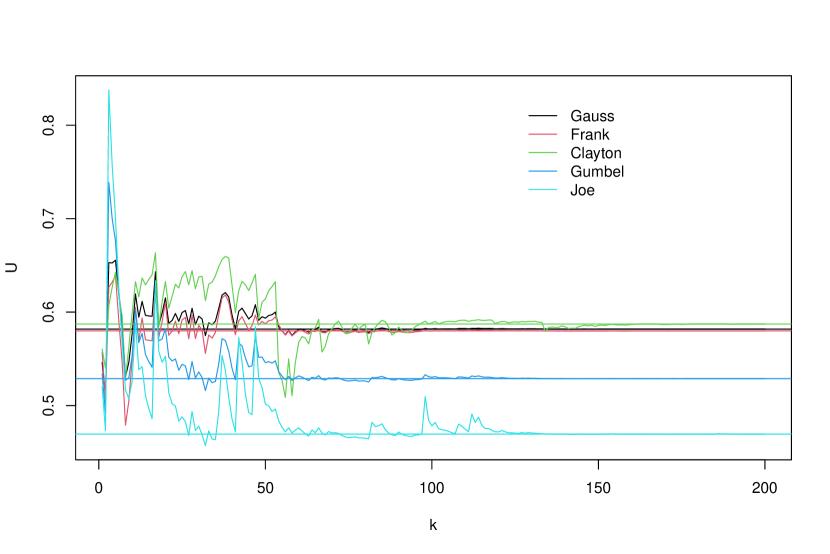
Figure 2: Plots of $(k,S_{k}(\bm{z}_{[n-k,n-1]},z_{n}))$ for $k\in\{1,\ldots,n-1\}$ for the copula filters of ARMA(1,1) models; see Example 4. Horizontal lines show ultimate values $S_{n-1}(\bm{z}_{[1,n-1]},z_{n})$.

Example 5 (Non-Gaussian ARFIMA(1,$d$,1) models).

In this example we consider s-vine copula processes sharing the kpacf of the ARFIMA(1,$d$,1) model with autoregressive parameter 0.95, moving-average parameter -0.85 and fractional differencing parameter $d=0.02$. The latter implies that the pacf of the Gaussian process satisfies $|\alpha_{k}|\sim 0.02/k$ as $k\to\infty$ (Inoue,, 2002). The lack of absolute summability means that the Gaussian copula process does not satisfy the conditions of Theorem 1. It is an unresolved question as to whether any of these processes is causal. Fixing $n=701$ we obtain Figure 3. For the realized series of innovations used in the picture, convergence appears to take place, but is extremely slow. The tail-dependent Clayton and Joe copulas appear to take longest to settle down.

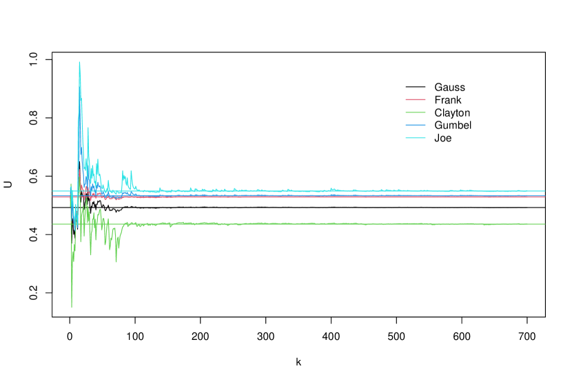
Figure 3: Plots of $(k,S_{k}(\bm{z}_{[n-k,n-1]},z_{n}))$ for $k\in\{1,\ldots,n-1\}$ for the copula filters of ARFIMA(1,$d$,1) models; see Example 5. Horizontal lines show ultimate values $S_{n-1}(\bm{z}_{[1,n-1]},z_{n})$.

An obvious practical solution that circumvents the issue of whether the infinite-order process has a convergent causal representation is to truncate the copula sequence $(C_{k})_{k\in\mathbb{N}}$ so that $C_{k}=C^{\perp}$ for $k>p$ for some relatively large but fixed value $p$. This places us back in the setting of ergodic Markov chains but, by parameterizing models through the kpacf, we preserve the advantages of parsimony.

5.3 An example with real data

For this example we have used data on the US CPI (consumer price index) taken from the OECD webpage. We analyse the log-differenced time series of quarterly CPI values from the first quarter of 1960 to the 4th quarter of 2020. The data are shown in the upper-left panel of Figure 4; there are $n=244$ observations.

To establish a baseline model we use an automatic ARMA selection algorithm and this selects an ARMA(5,1) model. We first address the issue of whether the implied Gaussian copula sequence in an ARMA(5,1) model can be replaced by Gumbel, Clayton, Frank or Joe copula sequences (or 180 degree rotations thereof); for any lag $k$ at which the estimated kpacf $\tau_{k}$ is negative we retain a Gaussian copula and so the non-Gaussian copula sequences are actually hybrid sequences with some Gaussian terms. The data $(x_{1},\ldots,x_{n})$ are transformed to pseudo-observations $(u_{1},\ldots,u_{n})$ on the copula scale using the empirical distribution function and the s-vine copula process is estimated by maximum-likelihood; this is the commonly used pseudo-maximum-likelihood method developed for general copula inference by Genest et al., (1995) and adapted to time series by Chen and Fan, (2006).

The best model results from replacing Gaussian copulas with Gumbel copulas and the improvement in the AIC is shown in the upper panel of Table 1; the improvement in fit is strikingly large. While the presented results relate to infinite-order processes, we note that very similar result (not tabulated) are obtained by fitting s-vine copula processes of finite order where the kpacf is truncated at lag 30. Parameter estimates for the infinite-order models are given in Table 2.

The residual QQ-plots in the middle row of Figure 4 give further insight into the improved fit of the process with Gumbel copulas. In the usual manner, residuals are reconstructions of the unobserved innovation variables. If $(\widehat{R}_{k})_{k\in\mathbb{N}}$ denotes the sequence of estimated Rosenblatt forward functions, implied by the sequence $(\widehat{C}_{k})_{k\in\mathbb{N}}$ of estimated copulas, then residuals $(z_{1},\ldots,z_{n})$ are constructed by setting $z_{1}=u_{1}$ and $z_{t}=\widehat{R}_{t-1}(\bm{u}_{[1,t-1]},u_{t})$ for $t>1$. To facilitate graphical analysis these are transformed onto the standard normal scale so that the QQ-plots in the middle row of Figure 4 relate to the values $(\Phi^{-1}(z_{1}),\ldots,\Phi^{-1}(z_{n})$ and are against a standard normal reference distribution. The residuals from the baseline Gaussian copula appear to deviate from normality whereas the residuals from the Gumbel copula model are much better behaved; the latter pass a Shapiro-Wilk test of normality (p-value = 0.97) whereas the former do not (p-value = 0.01).

	No. pars	AIC
Gaussian copula process	6	-184.62
Gumbel copula process	6	-209.28
Gaussian process	8	372.73
Gaussian copula process + skewed Student margin	10	352.50
Gumbel copula process + skewed Student margin	10	319.17

Table 1: Comparison of models by AIC: top panel relates to models for the pseudo-copula data $(u_{1},\ldots,u_{n})$ while the lower panel relates to full models of the original data $(x_{1},\ldots,x_{n})$.

	$\bm{\theta}^{\text{(Ga)}}$	s.e.	$\bm{\theta}^{\text{(Gu)}}$	s.e.
$\phi_{1}$	-0.381	0.104	-0.232	0.130
$\phi_{2}$	0.144	0.081	0.136	0.094
$\phi_{3}$	0.197	0.063	0.180	0.061
$\phi_{4}$	0.462	0.075	0.410	0.077
$\phi_{5}$	0.324	0.063	0.266	0.061
$\psi_{1}$	0.870	0.098	0.771	0.118

Table 2: Parameter estimates and standard errors for s-vine copula processes with Gaussian and Gumbel copula sequences fitted to the pseudo-copula data $(u_{1},\ldots,u_{n})$.

The picture of the kpacf in the top right panel of Figure 4 requires further comment. This plot attempts to show how well the kpacf of the fitted copula sequence matches the empirical Kendall partial autocorrelations of the data. The continuous line is the kpacf of the Gumbel/Gaussian copula sequence used in the best-fitting vine copula model of $(u_{1},\ldots,u_{n})$. The vertical bars show the empirical Kendall partial autocorrelations of the data at each lag $k$. However, the method should really be considered as ‘semi-empirical’ as it uses the fitted parametric copulas at lags $1,\ldots,k-1$ in order to construct the necessary data for lag $k$. The data used to estimate an empirical lag $k$ rank correlation are the points

$$\left\{\Big{(}\widehat{R^{(2)}}_{k-1}(\bm{u}_{[j-k+1,j-1]},u_{j-k}),\widehat{R}_{k-1}(\bm{u}_{[j-k+1,j-1]},u_{j})\Big{)},\quad j=k+1,\ldots,n\right\},$$

where $\widehat{R_{k}}$ and $\widehat{R^{(2)}}_{k}$ denote the estimates of forward and backward Rosenblatt functions; it may be noted that these data are precisely the points at which the copula density $c_{k}$ is evaluated when the model likelihood based on $c_{(n)}$ in (5) is maximized.

We next consider composite models for the original data $(x_{1},\ldots,x_{n})$ consisting of a marginal distribution and an s-vine copula process. The baseline model is simply a Gaussian process with Gaussian copula sequence and Gaussian marginal distribution. We experimented with a number of alternatives to the normal marginal and obtained good results with the skewed Student distribution from the family of skewed distributions proposed by Fernández and Steel, (1998). Table 1 contains results for models which combine the Gaussian and Gumbel copula sequences with the skewed Student margin; the improvement obtained by using a Gumbel sequence with a skewed Student margin is clear from the AIC values. The QQ-plots of the data against the fitted marginal distributions in the bottom row of Figure 4 also show the superiority of the skewed Student to the Gaussian distribution for this dataset.

The fitting method used for the composite model results in Table 1 is the two-stage IFM (inference functions for margins) method of Joe, (1997) in which the margin is estimated first, the data are transformed to approximately uniform using the marginal model, and the copula process is estimated by ML in a second step.

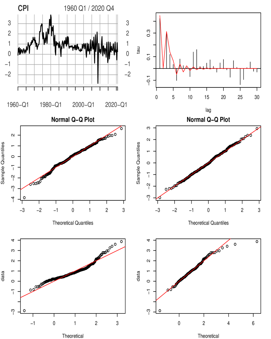
Figure 4: Top row: log-differenced CPI data and estimated kpacf of s-vine copula process using Gumbel copula sequence. Middle row: QQ-plots for residuals from models based on Gaussian (left) and Gumbel (right) copula sequences. Bottom row: QQ-plots of the data against fitted normal (left) and skewed Student (right) marginal distributions.

6 Conclusion

The s-vine processes provides a class of tractable stationary models that can capture non-linear and non-Gaussian serial dependence behaviour as well as any continuous marginal behaviour. By defining models of infinite order and using the approach based on the Kendall partial autocorrelation function (kpacf), we obtain a very natural generalization of classical Gaussian processes, such as Gaussian ARMA or ARFIMA.

The models are straightforward to apply. The parsimonious parametrization based on the kpacf makes maximum likelihood inference feasible. Analogues of many of the standard tools for time series analysis in the time domain are available, including estimation methods for the kpacf and residual plots that shed light on the quality of the fit of the copula model. By separating the issues of serial dependence and marginal modelling, we can obtain bespoke descriptions of both aspects that avoid the compromises of the more ‘off-the-shelf’ classical approach. The example of Section 5.3 indicates the kind of gains that can be obtained; it seems likely that many empirical applications of classical ARMA could be substantially improved by the use of models in the general s-vine class. In combination with v-transforms (McNeil,, 2021) s-vine models could also be used to model data showing stochastic volatility following the approach in Bladt and McNeil, (2021).

The approach we have adopted should also be of interest to theoreticians as there are a number of challenging open questions to be addressed. While we have proposed definitions of causality and invertibility for general s-vine processes, we currently lack a mathematical methodology for checking convergence of causal and invertible representations for sequences of non-Gaussian pair copulas.

There are some very interesting questions to address about the relationship between the partial copula sequence $(C_{k})_{k\in\mathbb{N}}$, the rate of convergence of causal representations and the rate of ergodic mixing of the resulting processes. The example of Figure 1 indicates that, even for a finite-order process, some very extreme models can be constructed that mix extremely slowly. Moreover, Example 5 suggests that non-Gaussian copula sequences serve to further elongate memory in long-memory processes and this raises questions about the effect of the tail dependence properties of the copula sequence on rates of convergence and length of memory.

It would also be of interest to confirm our conjecture that the pragmatic approach adopted in Section 5.2, in which the kpacf of the (infinite) partial copula sequence $(C_{k})_{k\in\mathbb{N}}$ is matched to that of a stationary and ergodic Gaussian process, always yields a stationary and ergodic s-vine model, regardless of the choice of copula sequence. However, for practical applications, the problem can be obviated by truncating the copula sequence at some large finite lag $k$, so that we are dealing with an ergodic Markov chain as in Section 3.

Appendix A Proofs

A.1 Proof of Proposition 1

In this proof we use the notation $(\bm{u})_{i}$ to denote the $i$th component of a vector $\bm{u}$ and $\bm{u}_{-i}$ to denote the vector $\bm{u}$ with $i$th component removed. An exchangeable copula satisfies $C_{k}(u,v)=C_{k}(v,u)$ for all $u,v$ and hence $h_{k}^{(2)}(u,v)=h_{k}^{(1)}(v,u)$. From this it follows that $R^{(2)}_{1}(u,x)=h_{1}^{(2)}(x,u)=h_{1}^{(1)}(u,x)=R_{1}(u,x)$. Part (i) follows by induction using the facts that for $\bm{u}=(u_{1},\ldots,u_{k})^{\top}\in(0,1)^{k}$ we have $(\overline{\bm{u}})_{k}=u_{1}$, $\overline{\bm{u}}_{-k}=(u_{k},\ldots,u_{2})^{\top}$ and $\overline{\overline{\bm{u}}_{-k}}=\bm{u}_{-1}$. We have that

$$R^{(2)}_{k}(\overline{\bm{u}},x) =h_{k}^{(2)}\Big{(}R^{(2)}_{k-1}(\overline{\bm{u}}_{-k},x),R_{k-1}(\overline{\bm{u}}_{-k},(\overline{\bm{u}})_{k})\Big{)}$$

$$=h_{k}^{(1)}\Big{(}R_{k-1}(\overline{\bm{u}}_{-k},u_{1}),R^{(2)}_{k-1}(\overline{\bm{u}}_{-k},x)\Big{)}=h_{k}^{(1)}\Big{(}R^{(2)}_{k-1}(\bm{u}_{-1},u_{1}),R_{k-1}(\bm{u}_{-1},x)\Big{)}=R_{k}(\bm{u},x).$$

For part (ii) we observe that for any $k>1$ the implication of part(i) is that for any $t,s\in\mathbb{N}$ the conditional distribution of $U_{t+k}\mid U_{t+1}=u_{1},\ldots,U_{t+k-1}=u_{k-1}$ is the same as that of $U_{s+1}\mid U_{s+2}=u_{k-1},\ldots,U_{s+k}=u_{1}$. It easily follows that $(U_{t+1},\ldots,U_{t+k})\stackrel{{\scriptstyle\text{\tiny d}}}{{=}}(U_{s+k},\ldots,U_{s+1})$ which proves reversibility of the process.

A.2 Proof of Proposition 2

If $(X_{t})$ is a Gaussian process its marginal distributions of all orders are multivariate Gaussian. The general d-vine copula decomposition in (1) can be applied to each $n$-dimensional marginal density. Since the conditional distributions of pairs $(X_{j-k},X_{j})$ given intermediate variables are bivariate Gaussian distributions with covariance matrices that do not depend on the conditioning variables, the simplifying assumption holds for each pair copula density in (1) (see also Joe,, 2015, pages 106–108). The stationarity assumption ensures that the joint density of the $n$-dimensional copula takes the form (5).

Conversely, an s-vine process with Gaussian marginal density and Gaussian pair copulas is a stationary process with $n$-dimensional marginal densities of the form (7). These are the densities of multivariate Gaussian distributions and the resulting process is a Gaussian process.

A.3 Proof of Proposition 3

Let $(Z_{k})_{k\in\mathbb{N}}$ be a sequence of iid standard uniform variables and $(U_{k})_{k\in\mathbb{N}}$ a sequence of uniform random variables generated by setting $U_{1}=Z_{1}$ and $U_{k}=R^{-1}_{k-1}\Big{(}(U_{1},\ldots,U_{k-1})^{\top},Z_{k}\Big{)}$ for $k>1$ where $(R_{k})_{k\in\mathbb{N}}$ denotes the sequence of Rosenblatt functions associated with the sequence of Gaussian pair copulas $(C_{k})_{k\in\mathbb{N}}$. Moreover, let $(X_{k})_{k\in\mathbb{N}}$ be a sequence of standard Gaussian variables defined by setting $X_{k}=\Phi^{-1}(U_{k})$ for all $k$.

It follows that, for any $k\geqslant 1$, $(X_{1},\ldots,X_{k+1})\sim N_{k+1}(\bm{0},P_{k+1})$ where $P_{k+1}$ is the $(k+1)$-dimensional correlation matrix implied by the acf $(\rho_{i})_{i\in\mathbb{N}}$ of $(X_{i})_{i\in\mathbb{N}}$ as in (14). The standard result for the conditional distribution of a multivariate normal implies that

$$X_{k+1}\mid X_{1}=x_{1},\ldots,X_{k}=x_{k}\sim N\Big{(}\overline{\bm{\rho}}_{k}^{\top}P_{k}^{-1}(x_{1},\ldots,x_{k})^{\top},\;1-\bm{\rho}_{k}^{\top}P_{k}^{-1}\bm{\rho}_{k}\Big{)},$$

where $\bm{\rho}_{k}=(\rho_{1},\ldots,\rho_{k})^{\top}$ as in (14) and $\overline{\bm{\rho}}_{k}$ is the reversed vector. The mean of the conditional distribution is the best linear predictor of $X_{k+1}$ and the variance of the conditional distribution is the mean squared prediction error; let us write the former as $\sum_{j=1}^{k}\phi^{(k)}_{j}x_{k+1-j}$, where $\phi^{(k)}_{j}=(P_{k}^{-1}\bm{\rho}_{k})_{j}$, and the latter as $\sigma_{k}^{2}$. We then have

$$R_{k}(\bm{u},x) = \mathbb{P}(U_{k+1}\leqslant x\mid U_{1}=u_{1},\ldots,U_{k}=u_{k})$$

$$= \mathbb{P}(X_{k+1}\leqslant\Phi^{-1}(x)\mid X_{1}=\Phi^{-1}(u_{1}),\ldots,X_{k}=\Phi^{-1}(u_{k}))$$

$$= \Phi\left(\frac{\Phi^{-1}(x)-\sum_{j=1}^{k}\phi^{(k)}_{j}\Phi^{-1}(u_{k+1-j})}{\sigma_{k}}\right).$$

The expression $\sigma_{k}^{2}=\prod_{j=1}^{k}(1-\alpha_{j}^{2})$ and the recursive formula (18) for the coefficients $\phi_{j}^{(k)}$ follow from the Durbin–Levinson Algorithm; see Brockwell and Davis, (1991), Proposition 5.2.1.

It follows from (17) that, for $k>0$,

$$U_{k+1}=R_{k}^{-1}((U_{1},\ldots,U_{k})^{\top},Z_{k+1})=\Phi\left(\sigma_{k}\Phi^{-1}(Z_{k+1})+\sum_{j=1}^{k}\phi^{(k)}_{j}\Phi^{-1}(U_{k+1-j})\right)$$ (25)

which may be written in terms of the variables $(X_{k})_{k\in\mathbb{N}}$ as $X_{k+1}=\sigma_{k}\epsilon_{k+1}+\sum_{j=1}^{k}\phi^{(k)}_{j}X_{k+1-j}$ where we introduce the further notation $\epsilon_{k}=\Phi^{-1}(Z_{k})$ for all $k\in\mathbb{N}$. An inductive argument then shows that this may be written in the form $X_{k+1}=\sigma_{k}\epsilon_{k+1}+\sum_{j=1}^{k}\psi^{(k)}_{j}\epsilon_{k+1-j}$ with the coefficients $\psi_{j}^{(k)}$ as defined in (20). Equation (22) then follows easily from (11).

A.4 Proof of Theorem 1

As in the proof of Proposition 3 we introduce the notation $(X_{t})_{t\in\mathbb{Z}}$ and $(\epsilon_{t})_{t\in\mathbb{Z}}$ where $X_{t}=\Phi^{-1}(U_{t})$ and $\epsilon_{t}=\Phi^{-1}(Z_{t})$. For fixed $k$ the formulas $U_{t}=S_{k}((Z_{t-k},\ldots,Z_{t-1})^{\top},Z_{t})$ and $Z_{t}=R_{k}((U_{t-k},\ldots,U_{t-1})^{\top},U_{t})$ translate to

$$X_{t}=\sum_{j=0}^{k}\psi^{(k)}_{j}\epsilon_{t-j}\quad\text{and}\quad\epsilon_{t}=\sum_{j=0}^{k}\tilde{\phi}^{(k)}_{j}X_{t-j}$$

where $\tilde{\phi}^{(k)}_{0}=1/\sigma_{k}$ and $\tilde{\phi}^{(k)}_{j}=-\phi^{(k)}_{j}/\sigma_{k}$ for $j>1$.

Debowski, (2007, Theorem 6) shows that under Assumption 3 the limiting representations

$$X_{t}=\sum_{j=0}^{\infty}\psi_{j}\epsilon_{t-j}\quad\text{and}\quad\epsilon_{t}=\sum_{j=0}^{\infty}\tilde{\phi}_{j}X_{t-j}$$ (26)

hold where $(\tilde{\phi}_{j})_{j\in\mathbb{Z}_{+}}$ and $(\psi_{j})_{j\in\mathbb{Z}_{+}}$ are sequences such that $\lim_{k\to\infty}\tilde{\phi}_{j}^{(k)}=\tilde{\phi}_{j}$ and $\lim_{k\to\infty}\psi_{j}^{(k)}=\psi_{j}$ and such that $\psi_{j}=\operatorname{cov}(X_{t},Z_{t-j})$, $\tilde{\phi}_{0}=1/\psi_{0}$ and $\sum_{j=0}^{k}\tilde{\phi}_{j}\psi_{k-j}=0$ for $k>0$; the series in the rhs of (26) converge absolutely, almost surely. Moreover, under Assumption 3 we also have that the terms $\sigma_{k}^{2}=\prod_{j=1}^{k}(1-\alpha_{j}^{2})$ converge to a finite limit $\sigma$ and so we can introduce a sequence $(\phi_{j})_{j\in\mathbb{N}}$ such that $\phi_{j}=-\sigma\tilde{\phi}_{j}$ and write

$$X_{t}=\sigma\epsilon_{t}+\sum_{j=1}^{\infty}\psi_{j}\epsilon_{t-j}\quad\quad\text{and}\quad\quad\epsilon_{t}=\sigma^{-1}X_{t}-\sigma^{-1}\sum_{j=1}^{\infty}\phi_{j}X_{t-j}.$$

Finally, by Proposition 3, equations (22) and (23) are seen to be a restatement of the latter formulas in terms of the Rosenblatt functions.

Appendix B Markov chain analysis

The Markov chain specified by (16) under Assumption 1 is a well-behaved example of a chain on a general state space. The properties of the process can be verified by standard arguments which are collected here for completeness.

Invariance.

The transition kernel of the Markov chain is given by

$$\mathsf{P}(\bm{u},A) =\mathbb{P}\left(\bm{U}_{2}\in A\mid\bm{U}_{1}=\bm{u}\right)=\mathbb{P}\left(F(\bm{U}_{1},Z)\in A\mid\bm{U}_{1}=\bm{u}\right)=\prod_{i=2}^{p}I_{\{u_{i}\in A_{i-1}\}}\int_{A_{p}}f_{p}(\bm{u},x)\mathrm{d}x$$

for a set $A=A_{1}\times\cdots\times A_{p}\subseteq\mathcal{X}$. Writing $\pi$ for the probability measure implied by $C_{(p)}$ and using (7), we have that

$$\int_{(0,1)^{p}}\pi(\mathrm{d}\bm{u})\mathsf{P}(\bm{u},A) =\int_{(0,1)^{p}}c_{(p)}(u_{1},\ldots,u_{p})\prod_{i=2}^{p}I_{\{u_{i}\in A_{i-1}\}}\left(\int_{A_{p}}f_{p}(\bm{u},x)\mathrm{d}x\right)\mathrm{d}\bm{u}$$

$$=\int_{0}^{1}\int_{A_{1}}\cdots\int_{A_{p-1}}c_{(p)}(u_{1},\ldots,u_{p})\left(\int_{A_{p}}f_{p}(\bm{u},x)\mathrm{d}x\right)\mathrm{d}u_{1}\cdots\mathrm{d}u_{p}$$

$$=\int_{0}^{1}\int_{A_{1}}\cdots\int_{A_{p}}c_{(p+1)}(u_{1},\ldots,u_{p},u_{p+1})\mathrm{d}u_{1}\cdots\mathrm{d}u_{p+1}$$

$$=\int_{A_{1}}\cdots\int_{A_{p}}c_{(p)}(u_{2},\ldots,u_{p},u_{p+1})\mathrm{d}u_{2}\cdots\mathrm{d}u_{p+1}=\pi(A)$$

showing that $\pi$ is an invariant measure.

Irreducibility.

A process is $\phi$-irreducible if there is a measure $\phi$ on $\mathcal{X}$ such that for every set $A\subseteq\mathcal{X}$ with $\phi(A)>0$ and every $\bm{u}\in(0,1)^{p}$ there exists $n=n(\bm{u},A)>0$ such that $\mathsf{P}^{n}(\bm{u},A)>0$. In our case it suffices to take $n=p$, independent of $\bm{u}$ and $A$, and $\phi$ to be Lebesgue measure. After $p$-fold iteration of the Markov updating scheme in (16) we obtain the random vector $\bm{U}_{p+1}=(U_{p+1},\ldots,U_{2p})^{\top}$ and for a set $A=A_{1}\times\cdots\times A_{p}$ with positive Lebesgue measure we have

$$\mathsf{P}^{p}(\bm{u},A) =\mathbb{P}(\bm{U}_{p+1}\in A\mid\bm{U}_{1}=\bm{u})$$

$$=\mathbb{P}(U_{p+1}\in A_{1},\ldots,U_{2p}\in A_{p}\mid U_{1}=u_{1},\ldots,U_{p}=u_{p})$$

$$=\int_{A_{1}}\cdots\int_{A_{p}}f_{U_{p+1},\ldots,U_{2p}\mid U_{1},\ldots,U_{p}}(x_{1},\ldots,x_{p}\mid u_{1},\ldots,u_{p})\mathrm{d}x_{1}\cdots\mathrm{d}x_{p}$$

and this probability is strictly positive if the integrand is strictly positive. Since the function in the integrand satisfies

$$f_{U_{p+1},\ldots,U_{2p}\mid U_{1},\ldots,U_{p}}(u_{p+1},\ldots,u_{2p}\mid u_{1},\ldots,u_{p}) =\prod_{j=1}^{p}f_{p}((u_{j},\ldots,u_{j+p-1})^{\top},u_{j+p})$$

and the conditional densities $f_{p}(\bm{u},x)$ as defined in (7) are products of strictly positive pair-copula densities, the result follows.

Recurrence.

Since the Markov chain is $\phi$-irreducible and admits an invariant probability measure, it is a positive recurrent chain. The absolute continuity of the transition kernel with respect to Lebesgue measure (exploited above) also means it is a Harris recurrent chain: for any point $\bm{x}\in\mathcal{X}$ and any set $A$ with invariant measure $\pi(A)=1$, either $\bm{x}\in A$ or, if not, $\mathsf{P}(\bm{x},A)=1$ so that it is certain that the time to entering $A$ is finite and this is a condition for Harris recurrence; see, for example, Roberts and Rosenthal, (2006, Theorem 6(v)).

Aperiodicity.

A periodic chain would cycle through $m\geqslant 2$ disjoint subsets of the state space $\mathcal{X}_{1},\ldots,\mathcal{X}_{m}$, each satisfying $\phi(\mathcal{X}_{i})>0$, in successive steps. If such behaviour were to occur we could find an $n\geqslant p$ such that $\mathsf{P}^{n}(\bm{u},\mathcal{X}_{2})=\mathbb{P}(\bm{U}_{n+1}\in\mathcal{X}_{2}\mid\bm{U}_{1}=\bm{u})=1$ for all $\bm{u}\in\mathcal{X}_{1}$, which would imply that $\mathsf{P}^{n}(\bm{u},\mathcal{X}_{1})=0$ for all $\bm{u}\in\mathcal{X}_{1}$. However, since $\phi(\mathcal{X}_{1})>0$, the argument used to establish the $\phi$-irreducibility of the process can be repeated to show that $\mathsf{P}^{n}(\bm{u},\mathcal{X}_{1})>0$ for all $\bm{u}\in\mathcal{X}$, which yields a contradiction.

References

- Aas et al., (2009) Aas, K., Czado, C., Frigessi, A., and Bakken, H. (2009). Pair-copula constructions of multiple dependence. Insurance: Mathematics and Economics, 44(2):182–198.
- Barndorff-Nielsen and Schou, (1973) Barndorff-Nielsen, O. and Schou, G. (1973). On the parametrization of autoregressive models by partial autocorrelation. Journal of Multivariate Analysis, 3(4):408–419.
- Beare, (2010) Beare, B. (2010). Copulas and temporal dependence. Econometrica, 78(395–410).
- Beare and Seo, (2015) Beare, B. and Seo, J. (2015). Vine copula specifications for stationary multivariate Markov chains. Journal of Time Series Analysis, 36:228–246.
- (5) Bedford, T. and Cooke, R. (2001a). Probabilistic Risk Analysis: Foundations and Methods. Cambridge University Press, Cambridge.
- (6) Bedford, T. and Cooke, R. M. (2001b). probability density decomposition for conditionally independent random variables modeled by vines. Annals of Mathematics and Artificial Intelligence, 32:245–268.
- Bedford and Cooke, (2002) Bedford, T. and Cooke, R. M. (2002). Vines–a new graphical model for dependent random variables. Annals of Statistics, 30(4):1031–1068.
- Bladt and McNeil, (2021) Bladt, M. and McNeil, A. J. (2021). Time series copula models using d-vines and v-transforms. https://arxiv.org/abs/2006.11088.
- Brechmann and Czado, (2015) Brechmann, E. C. and Czado, C. (2015). Copar—multivariate time series modeling using the copula autoregressive model. Applied Stochastic Models in Business and Industry, 31(4):495–514.
- Brockwell and Davis, (1991) Brockwell, P. J. and Davis, R. A. (1991). Time Series: Theory and Methods. Springer, New York, 2nd edition.
- Chen and Fan, (2006) Chen, X. and Fan, Y. (2006). Estimation of copula-based semiparametric time series models. Journal of Econometrics, 130(2):307–335.
- Cornfeld et al., (1982) Cornfeld, I., Fomin, S., and Sinai, G. (1982). Ergodic Theory. Springer-Verlag.
- Darsow et al., (1992) Darsow, W., Nguyen, B., and Olsen, E. (1992). Copulas and Markov processes. Illinois Journal of Mathematics, 36(4):600–642.
- Debowski, (2007) Debowski, L. (2007). On processes with summable partial autocorrelations. Statistics and Probability Letters, 77:752–759.
- Domma et al., (2009) Domma, F., Giordano, S., and Perri, P. F. (2009). Statistical modeling of temporal dependence in financial data via a copula function. Communications if Statistics: Simulation and Computation, 38(4):703–728.
- Fernández and Steel, (1998) Fernández, C. and Steel, M. (1998). On Bayesian modeling of fat tails and skewness. Journal of the American Statistical Association, 93(441):359–371.
- Genest et al., (1995) Genest, C., Ghoudi, K., and Rivest, L. (1995). A semi-parametric estimation procedure of dependence parameters in multivariate families of distributions. Biometrika, 82:543–552.
- Haff et al., (2010) Haff, H., Aas, K., and Frigessi, A. (2010). On the simplified pair copula construction - simply useful or too simplistic? Journal of Multivariate Analysis, 101:1296–1310.
- Hosking, (1981) Hosking, J. (1981). Fractional differencing. Biometrika, 68(1):165–176.
- Inoue, (2002) Inoue, A. (2002). Asymptotic behavior for partial autocorrelation functions of fractional ARIMA processes. The Annals of Applied Probability, 12(4):1471–1491.
- Joe, (1996) Joe, H. (1996). Families of m-variate distributions with given margins and m (m-1)/2 bivariate dependence parameters. Lecture Notes-Monograph Series, pages 120–141.
- Joe, (1997) Joe, H. (1997). Multivariate Models and Dependence Concepts. Chapman & Hall, London.
- Joe, (2006) Joe, H. (2006). Generating random correlation matrices based on partial correlations. Journal of Multivariate Analysis, 97:2177–2189.
- Joe, (2015) Joe, H. (2015). Dependence Modeling with Copulas. CRC Press, Boca Raton.
- Kurowicka and Cooke, (2006) Kurowicka, D. and Cooke, R. (2006). Uncertainty Analysis with High Dimensional Dependence Modelling. Wiley, Chichester.
- Liebscher, (2008) Liebscher, E. (2008). Construction of asymmetric multivariate copulas. Journal of Multivariate Analysis, 99:2234–2250.
- Loaiza-Maya et al., (2018) Loaiza-Maya, R., Smith, M., and Maneesoonthorn, W. (2018). Time series copulas for heteroskedastic data. Journal of Applied Econometrics, 33:332–354.
- Longla and Peligrad, (2012) Longla, M. and Peligrad, M. (2012). Some aspects of modeling dependence in copula-based Markov chains. Journal of Multivariate Analysis, 111:234–240.
- Maruyama, (1970) Maruyama, G. (1970). Infinitely divisible processes. Theory of Probability and its Applications, 15(1):1–22.
- McNeil, (2021) McNeil, A. J. (2021). Modelling volatile time series with v-transforms and copulas. Risks, 9(14).
- Meyn and Tweedie, (2009) Meyn, S. and Tweedie, R. L. (2009). Markov chains and stochastic stability. Cambridge University Press, 2nd edition edition.
- Nagler et al., (2020) Nagler, T., Krüger, D., and Min, A. (2020). Stationary vine copula models for multivariate time series. Working paper.
- Ramsey, (1974) Ramsey, F. (1974). Characterization of the partial autocorrelation function. Annals of Statistics, 2(6):1296–1301.
- Roberts and Rosenthal, (2006) Roberts, G. O. and Rosenthal, J. S. (2006). Harris recurrence of Metropolis-within-Gibbs and trans-dimensional Markov chains. The Annals of Applied Probability, 16(4):2123–2139.
- Samorodnitsky, (2007) Samorodnitsky, G. (2007). Long range dependence. Foundations and Trends in Stochastic Systems, 1(3):163–257.
- Smith et al., (2010) Smith, M., Min, A., Almeida, C., and Czado, C. (2010). Modeling Longitudinal Data Using a Pair-Copula Decomposition of Serial Dependence. Journal of the American Statistical Association, 105(492):1467–1479.