Auction Design with Data-Driven Misspecifications

Abstract

We consider auction environments in which at the time of the auction bidders observe signals about their ex-post value. We introduce a model of novice bidders who do not know know the joint distribution of signals and instead build a statistical model relating others’ bids to their own ex post value from the data sets accessible from past similar auctions. Crucially, we assume that only ex post values and bids are accessible while signals observed by bidders in past auctions remain private. We consider steady-states in such environments, and importantly we allow for correlation in the signal distribution. We first observe that data-driven bidders may behave suboptimally in classical auctions such as the second-price or first-price auctions whenever there are correlations. Allowing for a mix of rational (or experienced) and data-driven (novice) bidders results in inefficiencies in such auctions, and we show the inefficiency extends to all auction-like mechanisms in which bidders are restricted to submit one-dimensional (real-valued) bids.

Keywords: Belief Formation, Auctions, Efficiency
JEL Classification Numbers: D44, D82, D90

1 Introduction

In the standard model of auctions, bidders hold private information about the value of the object for sale. They commonly know how information is distributed across bidders, and every bidder $i$ correctly understands how bidder $j$ chooses his bid as a function of his private information. Every bidder best-responds to this correct understanding given the rules of the auction. The resulting strategy profile is a Bayes Nash Equilibrium.

A classic rationale for the correct understanding assumption in Bayes Nash Equilibrium is based on learning (see for example Dekel, Fudenberg, and Levine, 2004). If similar auctions are played many times (by different subjects in the roles of the various bidders), by looking at previous bids as well as what the corresponding bidders knew (at the time of the auction), one can recover the mapping from information to bids for past observations. If a steady state has been reached, this mapping will correctly describe behavior in the current auction, thereby supporting the rational expectation formulation.

But, access to previous bidders’ information is not so natural in practice. If the private information held by previous bidders is not disclosed, it is less clear how a novice bidder (who would only be exposed to data from past similar auctions played by others) would manage to have a correct understanding of other bidders’ strategies. A different modeling is required to describe the behavior of novice bidders in such a case.

To make progress in this unexplored direction, we consider one-object auctions in which at the time of the auction, bidder $i$’s private information is a noisy signal about his (own) ex post value for the good assumed to take one of finitely many realizations. We assume that after the auction is completed, what is publicly disclosed is the profile of bids as well as the ex post values for the various bidders, but not the signals observed by the bidders at the time of the auction. In the main part, we restrict attention to two-bidder auctions, but we note that our main insights carry over when there are more bidders.

It should be highlighted that we allow for correlations between signals, which will play a key role in the analysis. Moreover, despite the correlation, the setting is one of private values, since the distribution of bidder $i$’s ex post value is fully determined by bidder $i$’s signal (i.e., it is unaffected by the other bidder’s signal, conditional on $i$’s signal). Yet, novice players are assumed to be unaware of the true signal generating process, and thus of the private value character of the auction. Instead, they construct a representation of the statistical links between the variables of interest based on the signal they receive as well as the dataset available to them. Specifically, observations from past auctions take the form $(b_{1},v_{1},b_{2},v_{2})$ where $b_{j}$ is the bid previously submitted by a subject in the role of bidder $j$ and $v_{j}$ is his ex post value. A novice bidder $i$ constructs from the dataset the empirical distribution describing how $b_{j}$ is distributed conditional on the various possible ex post values of bidder $i$. He also uses his own signal $\theta_{i}$ about the likelihood of his various possible ex post values $v_{i}$ and combines the two to form a belief about how $(v_{i},b_{j})$ are jointly distributed given her own signal. He then best-responds to this belief given the rules of the auction.

We will be considering steady state environments in which there is a mixed population of bidders composed of a share of novice bidders (whose expectations are formed as just informally explained) and a complementary share of rational bidders assumed to have a correct understanding of the strategies of the two types of bidders as well as their respective share. Observe that rational bidders can alternatively be viewed as experienced bidders who would have had the opportunity to find out the best strategy in their auction environment (without necessarily an explicit knowledge of how the various types of bidders behave nor of the shares of the various types). We will refer to such steady states as Data-Driven Equilibria (see below for a discussion of how this concept relates to other existing concepts).

We apply this model to understand the efficiency properties of Data-Driven Equilibria, and more particularly, whether by a judicious choice of auction rule, one can implement an efficient allocation. This question resembles classic investigations in mechanism design with the main difference that our solution concept is not the Bayes Nash Equilibrium, but the Data-Driven Equilibrium designed to deal with the presence of novice bidders in our environment. Another departure from classic mechanism design is that for the main part of the paper, we will not be considering abstract mechanisms with arbitrary messages to be sent by bidders to the designer before an outcome (allocation and transfer) is decided. Instead, we will focus on what we call auction-like mechanisms defined as mechanisms in which each bidder submits a real-valued bid, and an outcome is chosen as a function of the profile of bids with the restriction that if a bidder submits a higher bid, this bidder has more chance of winning the object.

Our insights are as follows. Unless the distributions of signals of the two bidders are independent, data-driven bidders rely on a misspecified statistical model and as a result choose suboptimal bidding strategies. In Section 3, we start illustrating this with Second-Price Auctions (SPA) in the (symmetric) binary case in which there are two possible ex post values. We show that unlike rational bidders, novice bidders do not bid their expected value when there are correlations. As in winner’s curse models, novice bidders make inference about their ex post value from how the other bidder bids. In the case of positive correlation, this leads novice bidders to bid more than their expected value when they receive good signals (because in the neighborhood of large opponent’s bids, the own ex post value is more likely to be high) and less than their expected value when they receive bad signals (for a symmetric reason). We provide a numerical characterization of the equilibrium for a parametric class of distributions.

Clearly, the fact that novice and rational bidders do not bid in the same way leads to inefficiencies, unless there is perfect correlation of the signals, or the bidders are all novice or all rational. For our parametric example, we observe that the normalized welfare loss is U-shaped in the share of novice bidders as well as in the degree of correlation. More generally, we show for the binary mixed population case that as soon as there are correlations, there is some welfare loss in the Second Price Auction. We also consider First-Price Auctions (FPA), for which we also show that there must be inefficiencies whenever there is correlation. We illustrate through an example that sometimes the welfare loss may be larger in the Second-Price Auction than in the First-Price Auction.

Our main result concerns general auction-like mechanisms when ex post values can take at least three realizations. In Section 4, we provide a general inefficiency result. More precisely, we show in the mixed population case that for generic joint distributions of signals, there is no auction-like mechanism that allows to obtain an efficient outcome with probability one in any Data-Driven Equilibrium. The intuition for this result is as follows. To obtain efficiency among rational bidders, only the Second-Price Auction or a strategically equivalent auction format can be used because with more than two ex post values there is generically a manifold signal realizations corresponding to the same expected value for the object, but different beliefs about the signal realization of the other bidder. Since in Second-Price auctions, novice bidders do not bid their expected value as also observed in the simplified binary case, we conclude that inefficiencies must occur.

In Section 5, we put our analysis in perspective. First, we discuss alternative specifications of cognitive limitations in auction-like mechanisms either due to different accessibility to data sets from past auctions, or due to more or less sophisticated use of the same limited data sets. We make the simple observation that our main impossibility result would a fortiori hold if we were to consider a mixed population that includes extra cognitive types in addition to those considered in the main part of the paper.

Second, we discuss scenarios in which losing bids would not be accessible from past auctions, thereby considering a natural further restriction on the accessible data sets. We discuss various possible approaches to modeling novice bidders in this context, and suggest that all of them would lead to results similar to those obtained in our main model.

Third, we briefly discuss more general mechanisms beyond the auction-like mechanisms and note that judicious use of such mechanisms (direct mechanisms of the scoring rule type) may allow to elicit the beliefs of every bidder $i$ about bidder $j$’s (interim) type. Since in our baseline model, for generic distributions, no two different types have the same belief about their opponent’s type, such mechanisms could potentially be used to implement a broad range of allocation rules in the spirit of the work of Crémer and McLean (1988), Johnson, Pratt, and Zeckhauser (1990), McAfee and Reny (1992), and Gizatulina and Hellwig (2017). It should be mentioned however that such mechanisms are not commonly used in market design (perhaps because they require a level of knowledge -how the belief about opponent’s type relates to the valuation- that is rarely available to the designer). This consideration has led us to restrict attention to auction-like mechanisms which seem much more practical from a market design perspective.

Related literature

Our paper relates to different branches of literature. First, the modeling of data-driven bidders is in the spirit of the Analogy-Based Expectation Equilibrium (Jehiel, 2005) to the extent that these bidders aggregate the bid behavior of their opponent according to their own ex post value. Such an aggregation of bidding behavior can be related to the payoff-relevant analogy partition introduced in Jehiel and Koessler (2008). This modeling can also be related to the Bayesian Network Equilibrium (Spiegler, 2016), viewing these agents as believing that their values cause the bid of the opponent, but note that here the reasoning of novice bidders is viewed as a consequence of the nature of the dataset accessible to them, not as a consequence of a subjective wrong causality relation they could have in mind (see Spiegler (2020), and Jehiel (2020), for elaborations of the link between the Analogy-Based Expectation Equilibrium and the Bayesian Network Equilibrium).

Our paper is also related to the robust mechanism design literature (Bergemann and Morris, 2005), in the sense that a common motivation in that literature and our approach is that it may be hard to know what the beliefs of agents are. While the robust mechanism design literature uses this observation to motivate the desire to implement outcomes for a large range of (or even all) beliefs, our paper explicitly suggests a method of belief formation for bidders who do not have access to such information from past auctions. Our paper is also mostly concerned with a subclass of mechanisms that we refer to as auction-like mechanisms and how these perform in the joint presence of data-driven bidders and rational bidders, which has no counterpart in the literature on robust mechanism design.

Finally, from a technical point of view, our analysis makes use of some results developed in the literature on mechanism design with correlation. In particular, we borrow genericity arguments from Gizatulina and Hellwig (2017).

2 Model

Mechanisms

We consider the allocation of a single object to two bidders $i=1,2$ via an auction or more general auction-like mechanism. To simplify notation, when we consider a generic bidder $i\in\{1,2\}$, we denote the opponent by $j\neq i$. A Mechanism $M=\left[(B_{i}),q,p\right]$ consists of three elements: (i) feasible bids $B_{i}$ for the two bidders. A profile of bids is denoted $b=(b_{1},b_{2})\in B:=B_{1}\times B_{2}$. (ii) an allocation rule $q:B\rightarrow[0,1]^{2}$, $q(b)=(q_{1}(b),q_{2}(b))$, with $q_{1}(b)+q_{2}(b)\leq 1$, where $q_{i}(b)$ is the probability that bidder $i$ gets the object if the bid profile $b$ is submitted. (iii) A payment rule $t:B\rightarrow\mathbb{R}^{2}$, $p(b)=(p_{1}(b),p_{2}(b))$, where $p_{i}(b)$ denotes the payment bidder $i$ has to make if the bid profile $b$ is submitted.

Valuations

Ex-post, the value of the object for bidder $i$ is denoted $v_{i}$. It can take values in $V=\left\{v^{1},\ldots v^{K}\right\}$. $v_{i}$ can also be interpreted as the expected value based on a signal that is known ex-post if the ex-post value is not learned completely. Up to normalization, it is without loss to assume that $0=v^{1}<\ldots<v^{K}=1$. When participating in a mechanism, each bidder has an interim type $\theta_{i}=(\theta_{i}^{1},\ldots,\theta_{i}^{K})\in\Theta:=\Delta V$, where $\theta_{i}^{k}$ denotes the probability that $v_{i}=v^{k}$. A profile of types is denoted $\theta=(\theta_{1},\theta_{2})$. We assume that conditional on $\theta_{i}$, $v_{i}$ is independent of $\theta_{j}$. As a consequence the expected valuation of a bidder only depends on her own interim type: $E[v_{i}|\theta]=E[v_{i}|\theta_{i}]$. In other words, we are considering a setting with private values. Interim types are jointly distributed with distribution function $F(\theta)$ and density $f(\theta)$ defined over $\Theta^{2}$, and our main interest is in the case where $\theta_{1}$ and $\theta_{2}$ are not independent. We assume throughout that the joint distribution is symmetric and has a continuous and positive density. When there is no confusion, we slightly abuse notation and denote marginal distributions $F_{i}(\theta_{i})$ and $f_{i}(\theta_{i})$ by $F(\theta_{i})$ and $f(\theta_{i})$; and conditional distributions $F_{i}(\theta_{i}|\theta_{j})$ and $f_{i}(\theta_{i}|\theta_{j})$, by $F(\theta_{i}|\theta_{j})$ and $f(\theta_{i}|\theta_{j})$.

Rational and Misspecified Bidders

We assume that each bidder $i$ is characterized by a generalized type $t_{i}=\left(\theta_{i},s_{i}\right)$, where $\theta_{i}$ denotes the interim type described before, and $s_{i}\in\left\{r,m\right\}$ specifies the sophistication of the bidder. We denote the set of general types by $T=\Theta\times\{r,m\}$. For simplicity we will call $\theta_{i}$ just the type. The probability that $s_{i}=r$ is denoted $\lambda\in(0,1)$; we assume that it is independent of $\theta_{i}$ and across bidders. $s_{i}=r$ means that bidder $i$ is rational; and $s_{i}=m$ means that bidder $i$ is misspecified. Informally, the rational type correctly understands the environment, whereas the misspecified type holds beliefs that are endogenously determined by past observations of equilibrium outcomes of the mechanism she currently participates in. As we will see, this way of forming beliefs can lead to misspecifications, hence the name of the type.

We now make this precise. Fix a mechanism $M=\left[(B_{i}),q,p\right]$. A strategy of bidder $i$ is a function $b_{i}:T\rightarrow B_{i}$, where as a shorthand we write $b_{i}(\theta_{i},s_{i})=b_{i}^{s_{i}}(\theta_{i})$—that is, $b_{i}^{r}(\cdot)$ is the strategy of the rational type, and $b_{i}^{m}(\cdot)$ is the strategy of the misspecified type of bidder $i$. A strategy profile is denoted by $b=(b_{1},b_{2})=(b_{1}^{r},b_{1}^{m},b_{2}^{r},b_{2}^{m})$ and we denote the space of all strategy profiles by $\mathcal{B}$.

For a rational type of bidder $i$, the expected utility of type $\theta_{i}$ when submitting bid $b_{i}\in B_{i}$, and assuming that bidder $j$ bids according to $b_{j}(\cdot)$, is given by

$$U_{i}^{r}(b_{i},\theta_{i}|b_{j}(\cdot))=\mathbb{E}_{f}\left[v_{i}\,q_{i}(b_{i},b_{j}(\theta_{j},s_{j}))-p_{i}(b_{i},b_{j}(\theta_{j},s_{j}))|\theta_{i}\right],$$

where $\mathbb{E}_{f}$ is the expectation with respect to the correct distribution $f$ and the probability $\lambda$.

Next consider the misspecified type. We assume that this type forms a belief using past observations from the same mechanism played by similar bidders. Suppose the mechanism is run repeatedly with two (short-lived) bidders whose generalized type profiles are drawn i.i.d., across repetitions. If both bidders play according to a fixed strategy profile, as they would in a steady state, then repeated play generates a data set with observations $(b_{1},v_{1},b_{2},v_{2})$. We make the assumption that only bids and ex-post valuations are observable.

Assumption 1.

For each mechanism we consider, we assume that bidders have access to observations of the form $(b_{1},v_{1},b_{2},v_{2})$ from the same mechanism. The data about past mechanisms does not include the types $(\theta_{1},\theta_{2})$ of past bidders.

The idea behind this assumption is that bids are often disclosed after an auction and as time goes by, the ex-post valuation of the bidders, or an estimate thereof becomes known as well. On the other hand, bidders typically do not have access to the beliefs that past bidders in their role held at the time of bidding.

Past data allow bidders to identify the joint distribution of observable variables. We abstract from issues of estimation, and assume that bidders can recover this distribution without estimation error. The misspecified bidder then forms a simple model that combines relevant information from the empirical distribution of $(b_{1},v_{1},b_{2},v_{2})$, and her belief that her own $v_{i}$ is distributed according to $\theta_{i}$. To illustrate consider an auction with possible bids $B_{1}=B_{2}=[0,\infty)$. To assess the payoff from different bids, a bidder needs to know the joint distribution of her own valuation $v_{i}$ and the opponent’s bid $b_{j}$, conditional on her own type $\theta_{i}$. The misspecified bidder combines the distribution of $v_{i}$ given by her type $\theta_{i}$ with the joint distribution of $v_{i}$ and the opponent’s bid $b_{j}$ learned from the data in a parsimonious way, taking the joint distribution to be

$$\mathbb{P}_{m}\left[v_{i}=v^{k},b_{j}\leq b\middle|\theta_{i}\right]=\theta_{i}^{k}\times H_{i}(b|v^{k})$$ (1)

where $H_{i}(b|v^{k})$ is the c.d.f. of $b_{j}$ conditional on $v_{i}=v^{k}$ that is obtained from the data. Throughout, we will use $\mathbb{P}_{m}$ for probabilities assessed by the misspecified type and $\mathbb{P}_{f}$ for probabilities computed using the correct probabilistic model (given the density “$f$”). To see the difference in this particular example, note that

$$\mathbb{P}_{f}\left[v_{i}=v^{k},b_{j}\leq b\middle|\theta_{i}\right]=\theta_{i}^{k}\times\mathbb{P}_{f}\left[b_{j}\leq b\middle|\theta_{i},v_{i}=v^{k}\right]=\theta_{i}^{k}\times\mathbb{P}_{f}[b_{j}\leq b|\theta_{i}]$$

where the second equality follows from the assumption that $\theta_{j}$ and $v_{i}$ are independent, conditional on $\theta_{i}$. Under Assumption 1, $\mathbb{P}_{f}[b_{j}\leq b|\theta_{i}]$ cannot be assessed directly from the data since the types of past bidders are not available. In order to identify $\mathbb{P}_{f}[b_{j}\leq b|\theta_{i}]$ from the data, one would have to make assumptions about the strategies used by past bidders. These assumptions are ad hoc if only data on past bids and ex-post signals are available and a misspecified bidder does not have insight into the type of reasoning used by past bidders. The misspecified type therefore does not attempt to use the data through the lens of such assumptions but just takes the empirical correlation between $v_{i}$ and $b_{j}$ as given. One way to interpret the difference between the rational and the misspecified type is that the former is an experienced bidder who understands how bidders reason and is thus able to formulate the correct model to interpret the data where the latter lacks this understanding. In particular, the misspecified type does not know that conditional on her own type $\theta_{i}$, her own valuation is independent of the opponent’s type and thus her valuation and the opponents bid are also conditionally independent. The data available from past auctions, however, exhibits a correlation between the valuation $v_{i}$ and the bid $b_{j}$, since conditioning on the the unobserved type $\theta_{i}$ is not possible. This is the source of the misspecification of the $m$-type. As we will see, this gives rise to bidding behavior that is similar to the winner’s curse.

To summarize, for a misspecified type of bidder $i$, the expected utility of type $\theta_{i}$ when submitting bid $b_{i}\in B_{i}$, and assuming that bidder $j\neq i$ bids according to $b_{j}(\cdot)$, is given by

$$U_{i}^{m}(b_{i},\theta_{i}|b_{j}(\cdot)) =\mathbb{E}_{m}\left[v_{i}\,q_{i}(b_{i},b_{j}(\theta_{j},s_{j}))-p_{i}(b_{i},b_{j}(\theta_{j},s_{j}))|\theta_{i}\right],$$

$$=\sum_{k=1}^{K}\theta_{i}^{k}\int_{B_{j}}[v^{k}\,q_{i}(b_{i},b_{j})-p_{i}(b_{i},b_{j})]dH_{i}(b_{j}|v^{k}),$$

where $\mathbb{E}_{m}$ is the expectation formed according to the model described above. Note that in order to determine $H_{i}(\cdot|v^{k})$, it is enough to specify the strategy $b_{j}(\cdot)$ since $v_{i}$ and $b_{j}$ in the current auction do not depend on the bids placed by the bidder in role $i$ in the past. To understand this better, the example of the second-price auction in the next section will be helpful.

Equilibrium

To close the model, we assume that $H_{i}(\cdot|v^{k})$ are equilibrium objects that are generated by the equilibrium strategy profile and the misspecified type best-responds given her beliefs that are captured by $H_{i}(\cdot|v^{k})$.

Definition 1.

The strategy profile $b(\cdot)$ is a “Data-Driven Equilibrium” of the mechanism $M=\left[(B_{i}),q,t\right]$ if for all $i\neq j$, and for all $\theta_{i}\in\Theta$,

1. $b_{i}^{r}(\theta_{i})\in\arg\max_{b_{i}\in B_{i}}U_{i}^{r}(b_{i},\theta_{i}|b_{j}(\cdot))$,

2. $b_{i}^{m}(\theta_{i})\in\arg\max_{b_{i}\in B_{i}}U_{i}^{m}(b_{i},\theta_{i}|b_{j}(\cdot))$, where the distribution $H_{i}(b_{j}|v^{k})$ used to compute $U_{i}^{m}$ is derived from $\beta$, $f$, and $\text{Prob}[s_{i}=r]=\lambda$.

3 Standard Auctions

Before considering auction-like mechanisms and presenting the main result of the paper, we apply the model to standard auctions. This illustrates how data-driven beliefs affect bidding behavior.

In order to apply the model to standard auctions, we consider the case where $|V|=2$, so that the type of each bidder is one-dimensional. More specifically, we assume that $V=\{0,1\}$, so that the type can be written as one number $\theta_{i}\in[0,1]$, that specifies the probability that bidder $i$’s ex-post valuation is $v_{i}=1$. Note that this implies that $\theta_{i}$ is also the interim expected value of bidder $i$. In the following, we explain the equilibrium logic of our model for two standard auctions formats, the Second-Price Auction and the First-Price Auction. To compute concrete bidding equilibria, we will use a parametric class of joint distributions that allows us to vary the correlation between $\theta_{1}$ and $\theta_{2}$.

Example 1.

The joint density is given by

$$f(\theta_{1},\theta_{2})=\frac{2+\alpha}{2}\left(1-\left|\theta_{1}-\theta_{2}\right|\right)^{\alpha}.$$

The parameter $\alpha\in[0,\infty)$ determines the correlation between the two types where $\alpha=0$ corresponds to the independent case and $\alpha=\infty$ corresponds to perfect correlation. Figure 1 depicts the joint density for $\alpha\in\{.1,1,10\}$.

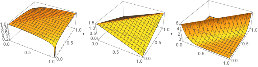
Figure 1: Joint density, $\alpha\in\{.1,1,10\}$ (left to right)

3.1 Second-price Auction

In a second-price auction, the rational type has a weakly dominant strategy since values are private. Hence she bids her interim expected value. We have

$$b^{r}(\theta_{i})=\theta_{i},$$

where $b^{r}$ refers to the rational type’s strategy. We denote the inverse by $\theta^{r}(b_{i})$, which is of course equal to $b_{i}$ in this case.

Now consider the misspecified type and consider a symmetric equilibrium, that is $b_{i}^{m}(\cdot)=b_{j}^{m}(\cdot)=b^{m}(\cdot)$. Suppose the equilibrium strategy $b^{m}(\cdot)$ is strictly increasing with inverse $\theta^{m}(b_{i})$. In equilibrium, the distribution of $b_{j}$ conditional on $v_{i}=1$ is

$$H^{\text{SPA}}(b\mid v_{i}=1)=\frac{\mathbb{P}_{f}\left[b_{j}\leq b,v_{i}=1\right]}{\mathbb{P}_{f}\left[v_{i}=1\right]},$$ (2)

where $H^{\text{SPA}}(\cdot)$ refers to this distribution for the SPA. Note that the misspecified type learns the correct joint distribution of $v_{i}$ and $b_{j}$ from the data. Hence we have used the correct probabilities $\mathbb{P}_{f}$ on the right-hand side. In the denominator, we have the unconditional probability of $v_{i}=1$ which is given by the (ex-ante) expectation of the random variable $\tilde{\theta}_{i}$. In the numerator, the probability $\mathbb{P}_{f}[b_{j}\leq b,v_{i}=1]$ is obtained by averaging $\mathbb{P}_{f}[b_{j}\leq b,v_{i}=1|\tilde{\theta}_{i}]$ over the (ex-ante) random variable $\tilde{\theta}_{i}$. Since $b_{j}$ is a function of $\theta_{j}$ and $s_{j}$, and the generalized type $(\theta_{j},s_{j})$ and $v_{i}$ are independent conditional on $\tilde{\theta}_{i}$, we have:

$$H^{\text{SPA}}(b\mid v_{i}=1) =\frac{\mathbb{E}_{\tilde{\theta}_{i}}\left[\mathbb{P}_{f}[b_{j}\leq b|\tilde{\theta}_{i}]\times\mathbb{P}_{f}[v_{i}=1|\tilde{\theta}_{i}]\right]}{\mathbb{E}[\tilde{\theta}_{i}]}$$

$$=\frac{\mathbb{E}_{\tilde{\theta}_{i}}\left[\left(\lambda\mathbb{P}_{f}[b^{r}(\theta_{j})\leq b|\tilde{\theta}_{i}]+(1-\lambda)\mathbb{P}_{f}[b^{m}(\theta_{j})\leq b|\tilde{\theta}_{i}]\right)\times\mathbb{P}_{f}[v_{i}=1|\tilde{\theta}_{i}]\right]}{\mathbb{E}[\tilde{\theta}_{i}]}$$

$$=\frac{1}{\mathbb{E}[\tilde{\theta}_{i}]}\int_{0}^{1}\left[\lambda F(b\mid\tilde{\theta}_{i})+(1-\lambda)F(\theta^{m}(b)\mid\tilde{\theta}_{i})\right]\tilde{\theta}_{i}\;f(\tilde{\theta}_{i})d\tilde{\theta}_{i}.$$

In the second line we decomposed the probability $\mathbb{P}_{f}[b_{j}\leq b|\tilde{\theta}_{i}]$ into the probability that a rational and a misspecified type bid below $b$, conditional on $\tilde{\theta}_{i}$. If the opponent is rational, the probability of $b_{j}\leq b$ is given by $\mathbb{P}_{f}[b^{r}(\theta_{j})\leq b|\tilde{\theta}_{i}]=F(\theta^{r}(b)\mid\tilde{\theta}_{i})=F(b\mid\tilde{\theta}_{i})$, and if the opponent is misspecified it is given by $\mathbb{P}_{f}[b^{m}(\theta_{j})\leq b|\tilde{\theta}_{i}]=F(\theta^{m}(b)\mid\tilde{\theta}_{i})$. The term $\tilde{\theta}_{i}$ in the third line is just $\mathbb{P}_{f}[v_{i}=1|\tilde{\theta}_{i}]$. We obtain a similar expression for the distribution of $b_{j}$ conditional on $v_{i}=0$:

$$H^{\text{SPA}}(b\mid v_{i}=0)=\frac{1}{\mathbb{E}[1-\tilde{\theta}_{i}]}\int_{0}^{1}\left[\lambda F(b\mid\tilde{\theta}_{i})+(1-\lambda)F(\theta^{m}(b)\mid\tilde{\theta}_{i})\right](1-\tilde{\theta}_{i})\;f(\tilde{\theta}_{i})d\tilde{\theta}_{i}$$

where the expectation in the integral differs from that in $H^{\text{SPA}}(b\mid v_{i}=1)$ since $P_{f}[v_{i}=0|\tilde{\theta}_{i}]=(1-\tilde{\theta}_{i})$, and outside the integral $\mathbb{E}[1-\tilde{\theta}_{i}]$ is the unconditional probability $P_{f}[v_{i}=0]$.

In a symmetric equilibrium of the second-price auction, the misspecified type’s bid for $\theta_{i}$ solves

$$\max_{b}\left\{\theta_{i}H^{\text{SPA}}(b\mid v_{i}=1)-\theta_{i}\int_{0}^{b}xdH^{\text{SPA}}(x|v_{i}=1)-(1-\theta_{i})\int_{0}^{b}xdH^{\text{SPA}}(x|v_{i}=0)\right\}$$

To obtain an equilibrium we have to determine a bidding strategy $b^{m}$ and the implied $H^{\text{SPA}}$ such that $b^{m}$ is optimal for the misspecified type give belief $H^{\text{SPA}}$. Taking the first-order condition for $b$ and substituting $H^{\text{SPA}}(b\mid v_{i}=1)$ and $H^{\text{SPA}}(b\mid v_{i}=0)$, we obtain a differential equation for $b^{m}$.

In Example 1, when $\alpha=0$—the independent case—we have that $H^{\text{SPA}}(b\mid v_{i}=1)=H^{\text{SPA}}(b\mid v_{i}=0)$ and the first order condition leads to $b^{m}(\theta_{i})=\theta_{i}$. But, when $\alpha$ differs from $0$, $H^{\text{SPA}}(b\mid v_{i}=1)$ differs from $H^{\text{SPA}}(b\mid v_{i}=0)$ and $b^{m}(\theta_{i})$ differs from $\theta_{i}$. Solving the differential equation numerically for the joint distribution from Example 1, we get the bid-functions illustrated in Figure 2.

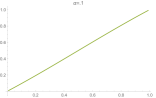
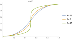
Figure 2: SPA bid-function $b_{m}(\theta_{i})$, $\alpha\in\{.1,1,10\}$ (left to right)

We see that increasing the correlation leads to stronger deviations from the rational bid. Moreover, the sensitivity of $b_{m}$ with respect to $\lambda$ becomes stronger if the correlation is stronger. Generally, for fixed correlation, increasing the share of misspecified types $(1-\lambda)$ leads to smaller deviation from rationality. Bidding against mainly rational types, a misspecified type’s behavior exhibits strong deviations from rationality, but in equilibrium, the presence of other misspecified types has a dampening effect.

Intuition

The reasoning leading to the derivation of $b^{m}$ follows a logic similar to that in classic analysis of winner’s curse models. We observe from Figure 2 that the misspecified type overbids for $\theta_{i}>1/2$ and underbids for $\theta_{i}<1/2$. What explains this behavior? To understand this, it is useful to shut down the (dampening) equilibrium effect of misspecified types and assume that $\lambda\approx 1$. The crucial observation is that the $m$-type believes that conditional on $v_{i}=1$, the opponent’s bid distribution is strong. This is because in the data, $v_{i}$ and $b_{j}$ are positively correlated: Observations with $v_{i}=1$ are more likely generated when $\tilde{\theta}_{i}$ is high. Due to the positive correlation between $\theta_{i}$ and $\theta_{j}$, this implies that $b_{j}$ is also likely to be high. Conversely, the $m$-type believes that conditional on $v_{i}=0$, the opponent’s bid distribution is weak.

For an $m$-type with low $\theta_{i}$, consider the incentives to decrease the bid below $b=\theta_{i}$. In this range reducing the bid has a large effect on the winning probability conditional on $v_{i}=0$ (the $m$-type believes that conditional on $v_{i}=0$, the opponents bid’s are concentrated on a low range) and little effect on the winning probability conditional on $v_{i}=1$ (where the $m$-type believes the opponents bid’s are concentrated on a high range). Therefore, the $m$-type believes that by shading the bid, she can cut the losses from winning with $v_{i}=0$, without a strong reduction of the gains from winning when $v_{i}=1$.

For a high $\theta_{i}$, this logic is reversed. Consider the incentives to increase the bid above $b=\theta_{i}$ when $\theta_{i}$ is high. The bid is now in a range where the $m$-type believes that increasing the bid mainly effects the winning probability conditional on $v_{i}=1$ and has little effect on the winning probability conditional on $v_{i}=0$. Hence, she thinks overbidding increases the profits from winning with $v_{i}=1$, while only modestly increasing the losses from winning with $v_{i}=0$. This leads to bids above $\theta_{i}$ for high types of the misspecified bidder.

Inefficiency of the Second-Price Auction

While the distortions observed in the example are specific to the parametric class of distributions, we can show generally that the SPA is not efficient whenever both rational and misspecified types arise with positive probability, and the types of the two bidders are correlated.

Proposition 1.

If $\lambda\in(0,1)$ and $\text{Corr}[\theta_{1},\theta_{2}]\neq 0$, then any equilibrium of the second-price auction in which the rational types of both bidder play their dominant strategies is inefficient.

Proof.

All omitted proofs can be found in Appendix A. ∎

Revenue and Efficiency

Continuing our illustration for the parametric class in Example 1, we show how revenue and (relative) efficiency of the allocation varies with (a) the share of rational types $\lambda$ and (b) the correlation between $\theta_{1}$ and $\theta_{2}$—that is the parameter $\alpha$.

Figure 3 plots the revenue as a function of $\lambda$ for different values of $\alpha$. Note that the comparison between different values of $\alpha$ with $\lambda$ held fixed is not very informative since the joint distribution changes in a complicated way as $\alpha$ changes.

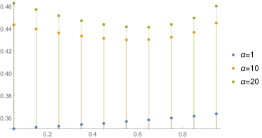
Figure 3: Revenue from the SPA as a function of $\lambda$: for $\alpha\in\{1,10,20\}$

We see that for the case of weak correlation ($\alpha=1$), revenue is increasing in the share of rational type. This suggests that the distortions in the misspecified type’s bidding function adversely affect revenue. For highly correlated interim types, the pattern changes and revenue is U-shaped in the share of rational types. The initial decline is intuitive since the distortions in the $m$-types bid become larger if the share of rational types increases. Profits rise again if the share of rational types becomes so large that presence of $m$-types becomes unlikely.

Figure 4 shows how efficiency changes depending on $\lambda$ and $\alpha$.

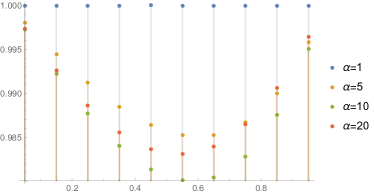
Figure 4: Efficiency of SPA as a function of $\lambda$: for $\alpha\in\{1,5,10,20\}$

To make this comparable across different parameter sets, we normalize efficiency by the expected ex-post value achieved if the object is always allocated to the bidder with the highest interim type. Clearly when $\lambda=0$ or $1$, there is no inefficiency given that bidders of the same sophistication bid in the same way. Moreover, both when $\alpha=0$ (the independent case) or $\alpha=\infty$ (perfect correlation) there is no inefficiency either. In the parametric example, we observe that the relative efficiency is $U$-shaped as a function of $\lambda$ and $\alpha$, as shown in Figure 5.

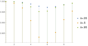
Figure 5: Efficiency of SPA as a function of $\alpha=1/5+5^{k}$ where $k=1,\ldots,9$ is on the horizontal axis. $\lambda\in\{.05,.5,.95\}$.

3.2 First-price auction

In a first price auction, we obtain the misspecified type’s belief in similar way as for the second price auction:

$$H^{\text{FPA}}(b\mid v_{i}=1) =\int_{0}^{1}\left[\lambda F(\theta^{r}(b)\mid\tilde{\theta}_{i})+(1-\lambda)F(\theta^{m}(b)\mid\tilde{\theta}_{i})\right]\tilde{\theta}_{i}\frac{f(\tilde{\theta}_{i})}{E[\tilde{\theta}_{i}]}d\tilde{\theta}_{i},$$

$$H^{\text{FPA}}(b\mid v_{i}=0) =\int_{0}^{1}\left[\lambda F(\theta^{r}(b)\mid\tilde{\theta}_{i})+(1-\lambda)F(\theta^{m}(b)\mid\tilde{\theta}_{i})\right](1-\tilde{\theta}_{i})\frac{f(\tilde{\theta}_{i})}{E[1-\tilde{\theta}_{i}]}d\tilde{\theta}_{i}.$$

$b^{r}(\cdot)$ and $b^{m}(\cdot)$ now denote the bidding strategies of the rational and misspecified types in the symmetric equilibrium of the FPA, and their inverses are denoted by $\theta^{r}(\cdot)$ and $\theta^{m}(\cdot)$. The misspecified bidder’s bid for type $\theta_{i}$ maximizes

$$\max_{b}\left(1-b\right)\theta_{i}H^{\text{FPA}}(b\mid v_{i}=1)-b(1-\theta_{i})H^{\text{FPA}}(b|v_{i}=0).$$ (3)

Again we obtain a differential equation for $b^{m}(\theta_{i})$. In contrast to the second price auction, however, we cannot assume that rational bidders bid their expected valuations. Instead they maximize

$$\max_{b}\left(\theta_{i}-b\right)\left(\lambda F(\theta^{r}(b)|\theta_{i})+(1-\lambda)F(\theta^{m}(b)|\theta_{i})\right)$$

This optimization problem reflects the complete awareness of the model by rational bidders. They use the correct distribution $f$, the share of rational types in the population, and the equilibrium bidding strategies of both the rational and the misspecified types when determining their optimal bids. The first-order condition for the rational type’s problem yields a second differential equation. To compute an equilibrium, we need to solve the system of two ODEs with the boundary condition $(b^{m}(0),b^{r}(0))=(0,0)$. This proves challenging even for the distributions in our example, since the system has a singular point at the boundary condition. However, we obtain a similar inefficiency result as we had for the SPA.

Proposition 2.

If $\lambda\in(0,1)$ and $\text{Corr}[\theta_{1},\theta_{2}]\neq 0$, then the symmetric equilibrium of the first-price auction is inefficient.

3.3 Comparison

We can compute the bidding equilibrium for both auction formats for the case of only rational bidders ($\lambda=1$) and only misspecified bidders $\lambda=0$. Figure 6 shows the bid functions $b_{k}^{s}$ where $k=1,2$ denotes first- or second-price auctions and $s=m,r$ denotes the misspecified or rational type.

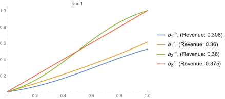
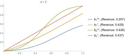
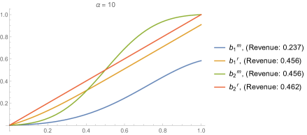
Figure 6: Equilibrium bid functions for $\alpha\in\{1,5,10\}$

To illustrate the role of correlation, the functions are shown for $\alpha\in\{1,5,10\}$. Comparing FPA and SPA in the rational case, we see the familiar revenue ranking that the SPA yields higher revenue than the FPA with correlated types. This revenue ranking is preserved in the case of misspecified bidders. Interestingly, with misspecified bidders, the gap between SPA and FPA becomes more pronounced if values are more correlated. This conforms well with the intuition for the distortions in the bid function: In the SPA low types underbid and high types overbid. In the FPA, the same forces lead the low types to underbid. But this allows the higher types to shade their bids more and the incentive to overbid does not compensate for this force. This leads to much lower bids for misspecified types compared to the rational equilibrium if the correlation is high.

Finally, we want to compare the efficiency of the SPA and FPA. This comparison is not interesting in the purely rational or purely misspecified cases since the symmetric equilibrium implies that both auction formats are fully efficient. A comparison in the mixed case is challenging because we are not able to compute the equilibrium in the FPA. To make progress we consider the best response of a misspecified type to the purely rational equilibrium. This allows us to show how efficiency changes if we inject a small share of misspecified types in a rational population. Figure 7 shows the resulting bidding strategies for $\alpha=1.5$.

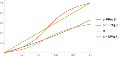
Figure 7: For the FPA ($k=1$), and the SPA ($k=2$), $b_{k}^{r}(\theta_{i})$ is the rational strategy if $\lambda=1$; $b_{k}^{m}(\theta_{i})$ is the best response of misspecified type to data generated by the purely rational equilibrium. ($\alpha=1.5$).

To compare the efficiency we numerically compute how much efficiency is lost in expectation if bidder one uses the purely rational strategy and bidder two uses the misspecified response. This number gives the rate at which efficiency decreases if we decrease $\lambda$ from $\lambda=1$. In the example depicted in Figure 7 we have a marginal loss of $.0035$ for the FPA and $.0088$ for the SPA. This means that the SPA is less efficient than the FPA.

4 Auction-like Mechanisms

We now consider the possibility of implementing an efficient allocation in the presence of both rational and misspecified buyers. We consider a class of auction-like mechanisms, in which bidders can place a one-dimensional bid $b\in B\subset\mathbb{R}$, and which allocate to the highest bid (possibly adjusted by a bonus or malus). We assume that bidders may choose not to participate in a mechanism in which case their utility is zero.

Definition 2.

An auction-like mechanism is given by $M=\left[B,\left(W_{i}\right)_{i=1,2},\left(L_{i}\right)_{i=1,2},\phi_{1}\right]$. $B=[\underline{b},\overline{b}]$ is the set of feasible bids. The allocation rule $\phi_{1}:B\rightarrow B$ is a strictly increasing function. The object is allocated to bidder 1 if $b_{1}>\phi_{1}(b_{2})$, to bidder two if $b_{1}<\phi_{1}(b_{2})$, and with probability $1/2$ if $b_{1}=\phi_{1}(b_{2})$. We denote the inverse by $\phi_{2}=\phi_{1}^{-1}$. The payment rules are $W_{i}:B\times B\rightarrow\mathbb{R}_{0}^{+}$, and $L_{i}:B\times B\rightarrow\mathbb{R}_{0}^{+}$, which specify the payment bidder $i$ has to make as a function of the bids, if she wins or loses, respectively. We assume that for each $i\in\{1,2\}$, both functions $W_{i},L_{i}$ are weakly increasing in bidder $i$’s own bid.
An auction-like mechanism is smooth if for $i\in\{1,2\}$, $\phi_{i}$, $W_{i}$, and $L_{i}$, are continuously differentiable with derivatives that can be continuously extended to the boundary of $B$.

The smoothness assumption is made for tractability. Many common auction formats are smooth auction-like mechanisms. Our main result is that if there are at least three possible ex-post valuations, then for generic type distributions, no smooth auction-like mechanism exists that has an efficient equilibrium.

To make this precise, we reformulate the types of agents. We denote the interim valuation of bidder $i$ with type $\theta_{i}$ by

$$w_{i}(\theta_{i}):=\mathbb{E}\left[v_{i}\middle|\theta_{i}\right].$$

Given the normalization $0=v^{1}<\ldots<v^{K}=1$, we have $w_{i}(\theta_{i})\in[0,1]$. For each $w_{i}\in[0,1]$, we denote the set of types $\theta_{i}$ that have interim valuation $w_{i}$ by

$$\Theta_{i}(w_{i}):=\left\{\theta_{i}\in\Theta_{i}\middle|\mathbb{E}\left[v_{i}\middle|\theta_{i}\right]=w_{i}\right\}.$$

For $w_{i}\in\{0,1\}$ this set is a singleton; and for all $w_{i}\in(0,1)$, there exists a homeomorphism $x_{i}(\cdot;w_{i}):\Theta_{i}(w_{i})\rightarrow[0,1]^{K-2}$, where $K=|V|$ is the number of ex-post valuations. We can therefore write the type of bidder $i$ as $(w_{i},x_{i})\in[0,1]^{K-1}$. While $w_{i}$ is the payoff-relevant part of the type, for $w_{i}\in(0,1),$ $x_{i}$ can be used to recover the belief $f(\theta_{j}|x_{i}^{-1}(x_{i};w_{i}))$ about bidder $j$’s type. Abusing notation we use $f(w_{1},x_{1},w_{2},x_{2})$ to denote the joint density of the buyers’ types and assume that this density is strictly positive.

Our main result is that for generic distributions, smooth auction-line mechanisms do not have efficient equilibria. To state this formally, we let $\mathcal{M}_{+}^{d}([0,1]^{2K-2})$ be the set of probability measures on $[0,1]^{2K-2}$ that admit continuous and strictly positive densities $f(w_{1},x_{1},w_{2},x_{2})$. We endow $\mathcal{M}_{+}^{d}([0,1]^{2K-2})$ with the uniform topology for densities. For given $V$ and $\lambda$, let $\mathcal{I}(V,\lambda)\subset\mathcal{M}_{+}^{d}([0,1]^{2K-2})$ be the set of prior distributions for which all equilibria of any smooth auction-like mechanism are inefficient.

Theorem 1.

Suppose $K=|V|\geq 3$ and $\lambda\in(0,1)$. Then for generic type distributions, there exists no smooth auction-like mechanism with an efficient equilibrium. Formally, $\mathcal{I}(V,\lambda)$ is a residual subset of $\mathcal{M}_{+}^{d}([0,1]^{2K-2})$, that is, it contains a countable intersection of open and dense subsets of $\mathcal{M}_{+}^{d}([0,1]^{2K-2})$.

The notion of genericity used here is the same as in Gizatulina and Hellwig (2017), who show the genericity of full surplus extraction. The key step in the proof is to show that in the presence of rational bidders, efficiency requires that the mechanism is a second price auction. The reason is that to achieve efficiency, the bid in an auction-like mechanism must be a function of $w_{i}$ only. If there are more than two ex-post valuations, for each $w_{i}\in(0,1)$, the set $\Theta(w_{i})$ is a manifold of dimension $K-2\geq 1$, and all types in $\Theta(w_{i})$ have identical interim expected valuations but different beliefs. We show that for generic distributions, the requirement that the bid is independent of the rational type’s belief, implies that the mechanism must be a second-price auction. We then finish the proof by extending the result of Proposition 1 to more than two ex-post valuations (see Lemma 6 below), showing that in a second-price auction the misspecified type does not bid truthfully, which rules out an efficient equilibrium.

Remark 1 (Two ex-post valuations).

With only two ex-post valuations ($K=2$), our proof does not apply. While the analysis of standard auctions in Section 3 suggests that bid functions of rational and misspecified types in auction-like mechanisms differ, it is an open question whether auction-like mechanism offer enough flexibility in choosing the payment rules so that types of both sophistication can be incentivised to use an identical bid function when $K=2$.

Remark 2 (More than two bidders).

The restriction to two bidders has been made for simplicity. With more than two bidders, we can consider misspecified types who have access to data from past auctions with observations of the form $(b_{1},v_{1},\ldots,b_{N},v_{N})$, where $N$ is the number of bidders. Such bidders will now rely on $h(b_{-i}|v_{i})$, the pdf of $b_{-i}=(b_{j})_{j\neq i}$ conditional on $v_{i}$, to form their beliefs about how variables of interest are distributed. We can define auction-like mechanisms that award the object to the highest bidder and specify payments as a function of all bids. We conjecture that the key argument in our proof—namely that efficiency requires the use of a second-price auction also works with more than two bidders, as long as there are at least two ex-post valuations. Moreover, an analogous result to Proposition 1 and Lemma 6 implies that misspecified types do not use the rational bid function in any equilibrium of the second-price auction.

4.1 Proof of Theorem 1

Regular Equilibria of Simple Mechanisms

First, we show that it suffices to consider regular equilibria of simple mechanisms. We call a smooth auction-like mechanism simple if it is of the form $M=\left[[0,1],\left(W_{i}\right),\left(L_{i}\right),Id\right]$, where $\phi=Id$ denotes the identity so that the allocation rule is symmetric. We call an equilibrium regular if it is symmetric and the bid of each generalized type $(w_{i},x_{i},s_{i})$ is given by a continuous and strictly increasing function $b(w_{i})$ with range $b([0,1])=[0,1]$. In other words, the bid only depends on the interim valuations, but not on the identity, sophistication, or belief $x_{i}$, of the bidder. Note that a regular equilibrium of a simple mechanism is efficient. We denote the strictly increasing and continuous inverse of $b(\cdot)$ by $\psi:[0,1]\rightarrow[0,1]$.

Lemma 1.

Let $\tilde{M}=[\tilde{B},(\tilde{W}_{i}),(\tilde{L}_{i}),\tilde{\phi}_{1}]$ be a smooth auction-like mechanism with an efficient equilibrium $(\tilde{b}_{1}(w_{1},x_{1},s_{1})$,$\tilde{b}_{2}(w_{2},x_{2},s_{2}))$. Then there exists a simple mechanism $M=\left[[0,1],\left(W_{i}\right),\left(L_{i}\right),Id\right]$, with a regular (and hence efficient) equilibrium.

Proof.

The proofs of all Lemmas can be found in the Appendix. ∎

In light of Lemma 1, it suffices to consider regular equilibria of simple mechanisms. The intuition behind this result is that in an efficient mechanism with a symmetric allocation rule, all bidders must use the same bids as function of their interim valuation. The proof shows that mechanisms for which the bidding function has discontinuities, these jumps can be removed in a way that preserves the smoothness of the payment rules. Lemma 1 falls short of the revelation principle because the full revelation argument may not preserve the smoothness of the payment rules if the equilibrium of the original mechanism is non-smooth.

Second-Price Auctions

Next we derive a condition on the payment rules and equilibrium bid function that characterizes regular equilibria of the second-price auction. We denote the equilibrium difference in utility between winning and losing of a bidder with bid $b=b(w_{i})$, whose bid is tied with the opponent by

$$\delta_{i}(b)=\psi(b)-\left(W_{i}(b,b)-L_{i}(b,b)\right).$$

In a regular equilibrium of the SPA, the rational type bids truthfully ($b(w)=w)$, and the payment rules satisfy $W_{i}(b,b)=b$ and $L_{i}\equiv 0$, so that $\delta_{i}(b)=0$ for all $b\in[0,1]$. The following Lemma shows the converse result.

Lemma 2.

Consider a simple mechanism $M=\left[[0,1],\left(W_{i}\right),\left(L_{i}\right),Id\right]$ with a regular equilibrium. If $\delta_{i}(b)=0$, for $i\in\{1,2\}$ and all $b\in[0,1]$, then $M$ is a second-price auction—that is, for all $i\in\{1,2\}$, $L_{i}(b_{i},b_{j})=0$ for all $b_{i}\leq b_{j}$ and $W_{i}(b_{i},b_{j}(w_{j}))=w_{j}$ whenever $b_{i}\geq b_{j}(w_{j})$.

Differentiability of the Bidding Strategy

To show that $\delta_{i}(b)=0$ for all bids we derive an implication of $\delta_{i}(b)>0$ and show that it is violated generically. In the derivations we will use first-order conditions and the following Lemma shows that the inverse of the bid function, $\psi(b)$ is differentiable if $\delta_{i}(b)>0$. The Lemma is based on the proof of Lemma 7 in Lizzeri and Persico (2000).

Lemma 3.

If $\delta_{i}(b_{0})>0$ for some $b_{0}\in[0,1]$, then there exist a non-empty interval $(\alpha,\beta)\subset[0,1]$, with $b_{0}\in(\alpha,\beta)$, such that $\psi$ is continuously differentiable on $(\alpha,\beta)$, and $\psi^{\prime}(b)>0$ and $\delta_{i}(b)>0$ for all $b\in(\alpha,\beta)$.

For generic distributions efficiency requires $M=SPA$.

Next, we show that $\delta_{i}(b)>0$ implies that a condition similar to the full-surplus extraction condition (McAfee and Reny, 1992) must be violated, and prove results analog to Gizatulina and Hellwig (2017, henceforth GH17), to show that for generic prior densities $f(w_{1},x_{1},w_{2},x_{2})$, we must have $\delta_{i}(b)=0$ for all $b\in[0,1]$, $i\in\{1,2\}$, and any regular equilibrium of a simple mechanism.

We begin by deriving an implication of $\delta_{i}(b)>0$. Fix $b\in(0,1)$ such that $\delta_{i}(b)>0$ and consider a rational bidder $i$ with type $(w_{i},x_{i})$, where $w_{i}=\psi(b)$ and $x_{i}\in X$ is arbitrary. In a regular equilibrium, this type maximizes (where we use $j\neq i$ to denote the opponent):

$$\max_{b^{\prime}\in[0,1]}\int_{0}^{\psi(b^{\prime})}\left(\psi(b)-W_{i}(b^{\prime},b(w_{j}))\right)f(w_{j}|\psi(b),x_{i})dw_{j}-\int_{\psi(b^{\prime})}^{1}L_{i}(b^{\prime},b(w_{j}))f(w_{j}|\psi(b),x_{i})dw_{j}$$

Given Lemma 3, we can differentiate the objective function with respect to $b^{\prime}$, and obtain the first-order condition, which must hold for $b^{\prime}=b$:

$$f(\tilde{w}_{j}=\psi(b)|\tilde{w}_{i}=\psi(b),x_{i})=\int_{0}^{1}\frac{\partial P_{i}(b,b(w_{j}))/\partial b_{i}}{\delta_{i}(b)\psi^{\prime}(b)}f(w_{j}|\tilde{w}_{i}=\psi(b),x_{i})dw_{j},$$ (4)

where we simplify notation by denoting the payment of bidder $i$ as follows

$$P_{i}(b_{i},b_{j}):=\boldsymbol{1}_{\{b_{i}>b_{j}\}}W_{i}(b_{i},b_{j})+\boldsymbol{1}_{\{b_{i}<b_{j}\}}L_{i}(b_{i},b_{j}).$$

Multiplying (4) by $f(\tilde{w}_{i}=\psi(b),x_{i})/f(\tilde{w}_{i}=\tilde{w}_{j}=\psi(b))$, and using

$$f(x_{i}|\tilde{w}_{i}=\tilde{w}_{j}=\psi(b))f(\tilde{w}_{i}=\tilde{w}_{j}=\psi(b))=f(x_{i},\tilde{w}_{i}=\tilde{w}_{j}=\psi(b)),$$

we obtain for all $x_{i}\in X_{i}$:

$$f(x_{i}|\tilde{w}_{i} =\tilde{w}_{j}=\psi(b))=\int_{0}^{1}m(b,\psi(b),w_{j})f(x_{i}|\tilde{w}_{i}=\psi(b),w_{j})dw_{j},$$ (5)

where

$$m(b,\psi(b),w_{j})=\frac{\partial P_{i}(b,b(w_{j}))/\partial b_{i}f(\tilde{w}_{i}=\psi(b),w_{j})}{\delta_{i}(b)\psi^{\prime}(b)f(\tilde{w}_{i}=\tilde{w}_{j}=\psi(b))}.$$

Since we consider a simple mechanism and prior densities $f\in\mathcal{M}_{+}^{d}([0,1]^{2K-2})$, and $\psi^{\prime}(b)>0$, the term $m(b,\psi(b),w_{j})$ is finite and non-negative. For fixed $b$, $m(b,\psi(b),\cdot)$ is in fact a probability density on $[0,1]$.

Condition (5) states that the density $f(\cdot|\tilde{w}_{i}=\tilde{w}_{j}=\psi(b))$ can be expressed as a positive linear combination of the densities $f(\cdot|\tilde{w}_{i}=\psi(b),w_{j})$ for $w_{j}\in[0,1]$, with positive weights on $w_{j}\neq\psi(b)$. By virtually the same proof as for Theorem 2.4 in GH17, we can show that for generic distributions (5) is violated.

To state the result we need several definitions that mimic GH17. Let $\mathcal{M}_{+}^{d}(X)$ be the set of absolutely continuous probabilities measures on $X$ with strictly positive and continuous densities, endowed with the topology induced by the $\sup$-norm for density functions on $X$; let $\mathcal{C}([0,1],\mathcal{M}_{+}^{d}(X))$ be the set of continuous mappings from $[0,1]$ to $\mathcal{M}_{+}^{d}(X)$, endowed with the topology of uniform convergence; and let $\mathcal{M}([0,1])$ be the set of probability measures on $[0,1]$, endowed with a topology that is metrizable by a metric that is a convex function on $\mathcal{M}([0,1])\times\mathcal{M}([0,1])$. Finally let $\mathcal{E}(w_{i})\subset\mathcal{C}([0,1],\mathcal{M}_{+}^{d}(X))$ be the set of continuous mappings that map $w\in[0,1]$ to densities $g(\cdot|w)\in\mathcal{M}_{+}^{d}(X)$ that satisfy the following condition: For all $\mu\in\mathcal{M}([0,1])$:

$$g(x_{i}|w_{i})=\int_{0}^{1}g(x_{i}|w^{\prime})\mu(dw^{\prime}),\;\forall x_{i}\in X\qquad\implies\qquad\mu=\delta_{w_{i}}$$ (6)

where $\delta_{w_{i}}\in\mathcal{M}([0,1])$ is the Dirac measure with a mass-point on $w_{i}$.

Lemma 4 (see Theorem 2.4 in Gizatulina and Hellwig, 2017).

For any $w_{i}\in(0,1)$, the set $\mathcal{E}(w_{i})$ is a residual subset of $\mathcal{C}([0,1],\mathcal{M}_{+}^{d}(X))$, that is, it is a countable intersection of open and dense subsets of $\mathcal{C}([0,1],\mathcal{M}_{+}^{d}(X))$.

The implication of this Lemma is that for fixed $w_{i}\in(0,1)$, and generic functions $w_{j}\mapsto f(\cdot|w_{i},w_{j})$ that map $w_{j}$ to conditional densities $f(\cdot|w_{i},w_{j})$, any simple mechanism with a regular equilibrium must satisfy $\delta_{i}(b(w_{i}))=0$.

This Lemma is insufficient for our purposes for two reasons. First, we need to show that for generic priors, the function that maps $w_{j}$ to the conditional density $f(x_{i}|w_{i},w_{j})$ is an element of $\mathcal{E}(w_{i})$, and second we need to show this for all $w_{i}$. To this end, for $i\in\{1,2\}$ let $\mathcal{W}_{i}$ be a countable and dense subset of $(0,1)$. We show that for generic prior densities $f(w_{1},x_{1},w_{2},x_{2})$, the mapping that maps $w_{j}\in[0,1]$ to the conditional density $f_{i}(\cdot|w_{i},w_{j})$ is an element of $\mathcal{E}_{i}(w_{i})$ for all $w_{i}\in\mathcal{W}_{i}$ and all $i\in\{1,2\}$. For the following Lemma, recall that $\mathcal{M}_{+}^{d}([0,1]^{2K-2})$ denotes the set of priors with strictly positive and continuous densities.

Lemma 5 (see Theorem 2.7 in Gizatulina and Hellwig, 2017).

For $i\in\{1,2\}$, let $\mathcal{W}_{i}$ be a countable and dense subset of $(0,1)$. Let $\mathcal{F}$ be the set of prior densities in $\mathcal{M}_{+}^{d}([0,1]^{2K-2})$ such that for all $i\in\{1,2\}$ and $w_{i}\in\mathcal{W}_{i}$, the mapping $w_{j}\mapsto f(\cdot|w_{i},w_{j})$ is an element of $\mathcal{E}(w_{i})$. Then $\mathcal{F}$ is a residual subset of $\mathcal{M}_{+}^{d}([0,1]^{2K})$, that is it contains a countable intersection of open and dense subsets of $\mathcal{M}_{+}^{d}([0,1]^{2K})$.

This Lemma implies that for generic prior densities $f(w_{1},x_{1},w_{2},x_{2})$, any regular equilibrium of a simple mechanism must satisfy $\delta_{i}(b(w_{i}))=0$ for all $w_{i}\in\mathcal{W}_{i}$. Since the functions $b(\cdot)$ and $\delta_{i}(\cdot)$ are continuous and $\mathcal{W}_{i}$ is dense, this implies $\delta_{i}(b)=0$ for all $b\in[0,1]$. By Lemma 2, this implies that for generic distributions, if a simple mechanism has a regular equilibrium, then it must be the second-price auction.

Bidding Strategy of the Misspecified Type in the Second-Price Auction

So far we have made use of the rational type’s first-order condition to show that efficiency cannot be achieved with an auction-like mechanism other than the SPA. To conclude the proof of Theorem 1 we show that for generic distributions, misspecified types do not use $b(w)=w$ in a SPA.

Lemma 6.

Let $\lambda\in(0,1)$ and suppose that $\mathbb{E}_{f}\left[\theta_{i}^{K}|w_{j}\leq b\right]\neq\frac{\mathbb{E}_{f}\left[\theta_{i}^{K}\right]}{\mathbb{E}_{f}\left[\theta_{i}^{1}\right]}\mathbb{E}_{f}\left[\theta_{i}^{1}|w_{j}\leq b\right]$ for some $i\in\{1,2\}$ and $b\in[0,1]$. In any equilibrium of the second price auction where the rational types bid truthfully, some types $(\theta_{i},m_{i})$ place a bid different from their interim valuation.

It is easy to see that the subset of prior densities for which there exists $i\in\{1,2\}$ and $b\in[0,1]$ such that $\mathbb{E}_{f}\left[\theta_{i}^{K}|w_{j}\leq b\right]\neq\frac{\mathbb{E}_{f}\left[\theta_{i}^{K}\right]}{\mathbb{E}_{f}\left[\theta_{i}^{1}\right]}\mathbb{E}_{f}\left[\theta_{i}^{1}|w_{j}\leq b\right]$ is open and dense $\mathcal{M}_{+}^{d}([0,1]^{2K})$ so that its intersection with $\mathcal{F}$ is residual by Lemma 5. This concludes the proof of Theorem 1.

5 Discussion and Extensions

In this section we discuss alternative modeling approaches and extensions. In Subsection 5.1, we discuss alternative models of belief formation from observed data when past bids and ex-post valuations are observable. In Subsection 5.2 we review possible approaches one could take for situations in which data from past auctions only include the winning bid or the payment made in past auctions. Finally, in Subsection 5.3 we discuss general mechanisms that go beyond the auction-like class considered in Section 4.

5.1 Model of Belief Formation from Observed Data

Our goal in this paper was to model belief formation of novice bidders (the $m$-types) who lack a complete understanding of the auction environment. Two basic assumptions have guided our modeling choices. First, we have assumed that novice bidders are sophisticated in the sense that they are able to use the empirical joint distribution of observable variables to inform their own bid. Second, we have assumed that novice bidders do not reason about how the bids of past bidders were formed. In particular they do not form a conjecture or model of the information available to past bidders and do not try to analyze how such information drives observed behavior.

Due to missing data about signals (or types) of past bidders, novice bidders are not able to learn the true joint distribution of signals/types, ex-post valuations and opponent’s bids. At the same time, a novice bidder knows her own type $\theta_{i}$, and has access to the empirical distribution of observable variables. She lacks knowledge how these two should be combined, and a priori, many different ways of using the data are conceivable, all of which rely on some implicit or explicit assumptions. Following our second basic assumption, novice bidders do not try to reason about how past bidders have determined their bids. Instead they simply combine the joint distribution of observable variables $v_{i}$ and $b_{j}$ with the belief about the distribution of $v_{i}$ given by their type $\theta_{i}$ to evaluate the expected payoff of different bids. This leads to a misspecified model in which $v_{i}$ and $b_{j}$ are correlated even when conditioning on $\theta_{i}$.

We believe that this simple way of using the data is a plausible model of an inexperienced bidder, but we do not want to claim that it is the only way to think about data-driven belief formation. It is an empirical question which models of belief formation are most suitable and we hope that this article inspires experimental or empirical work on this topic. In our model, other ways of forming beliefs may lead to different misspecifications and deviations from rational behavior. However, it is clear from the analysis in Section 4, that our main result is robust to the inclusion of various other forms of misspecifications. In fact the presence of various types who differ in their misspecification will make it harder to achieve efficiency since a mechanism would have to account for all types, a task that is already impossible in the presence for rational and a single misspecified type.

One aspect in which bidders could differ is the precision of the available data. For example, past bids may only be available in broad categories, such as “high” or “low” which would indicate that the bid was above or below some threshold $b^{\ast}$. A bidder with access to such aggregated data would have to make some assumption about the non-identified distribution of the bid on the intervals $[0,b^{\ast}]$ and $[b^{\ast},1]$. A simple starting point could be the uniform distribution but bidders may also make a different assumption. Given such an assumption, our notion of equilibrium can be adapted. While an analysis is beyond the scope of this paper, we conjecture that it would lead to similar conclusions as our present model.

Alternatively, one could consider different degrees of sophistication of novice bidders. We assume that novice bidders do not try to reason about how past bidders determined their bids, nor about the possible joint distribution of $v_{i},b_{j}$ and $\theta_{i}$. Novice bidders are sophisticated in their ability to analyze data, but boundedly rational in the sense that they do not question their method even though there might be alternative ways of using past data to perform bids.

Thinking about more sophisticated types, we may ask what additional knowledge they would need to have in order to see that their model is misspecified. In the data, one can see that $v_{i}$ and $b_{j}$ are independent conditional on $b_{i}$ since bids are a function of $\theta_{i}$. However, without further assumptions how past bids were formed, this does not allow to conclude that $v_{i}$ and $b_{j}$ are independent conditional on $\theta_{i}$. Hence, given the available data, it is not obvious to an observer or the novice bidder, that the $m$-type in our model uses a misspecified model. A “more sophisticated” type would therefore have to have access to more data that would allow to validate structural assumptions about past bids.

Conversely, we may think of less sophisticated types who have access to the same data as our $m$-type but do not attempt or are unable to use the statistical link between the $b_{j}$ and $v_{i}$. For example this could be bidders who are not able to analyze large data sets beyond producing marginal distributions of the opponents bids. Alternatively, the bidder may know her expected valuation $E[v_{i}|\theta_{i}]$ but not the full distribution $\theta_{i}$ over ex-post valuations. Such bidders may in some cases actually display less bias in their bidding behavior since they do not use the statistical link between the $b_{j}$ and $v_{i}$ that gives rise to a (perceived) conditional correlation. For example, this is the case in second price auctions in which such bidders would bid optimally, in contrast to the $m$-type bidders we consider.

5.2 Non-observability of losing bids and valuations

In this paper we have followed the paradigm that data on past beliefs is unobservable but bidders have full access to past bids and past ex-post valuations. In practice, the ex-post valuations may not be observed precisely, and perhaps only noisy signals of the true valuation are available. To model such a situation, one could formulate the type $\theta_{i}$ as a distribution over such signal realizations and proceed as before.

More importantly, auctioneers may not disclose all bids in an auction. In the following, we discuss possible approaches for the case that only the winning bid and the identity of the winner is observable (as well as ex-post valuations of both bidders). Alternatively, the auctioneer may disclose the identity of the winner and the payment she has to make. In first-price auction this is equivalent to disclosing the winning bid but in an ascending auction or second-price auction, the payment is equal to the second highest bid and the following discussion has to be modified accordingly.

Consider the case that after an auction with $b_{i}>b_{j}$, the data point $(i,b_{i},v_{i},v_{j})$ is observed, so that data about losing bids is not available. In the present paper, we have taken $H(b_{j}|v_{i})$ to be the empirical distribution of the opponent’s bid $b_{j}$ conditional on valuation $v_{i}$ for bidder $i$. If losing bids are not observed, this distribution is not directly accessible. We outline three exemplary models of how a bidder may construct $H(b_{j}|v_{i})$ that reflect different degrees of sophistication. For each approach, the constructed $H(b_{j}|v_{i})$ can be plugged into our equilibrium framework and the analysis would proceed as before.

A naive bidder may ignore that the observations about opponent’s bids $b_{j}$ for a given valuation $v_{i}$ is selected and use the (observable) distribution $H(b_{j}|v_{i},b_{j}>b_{i})$ instead of $H(b_{j}|v_{i})$. This approach will lead bidder $i$ to think that bidder $j$ bids higher than in reality, which creates additional bias.

A semi-naive bidder may be aware that for each $v_{i}$ she only observes a selected sample of opponent’s bids $b_{j}$ which satisfy $b_{j}>b_{i}$. For all other observations with a given $v_{i}$, $b_{i}$ is known and she can only infer that $b_{j}<b_{i}$. The bidder could then attempt to complete the missing data by assuming some distribution $\tilde{H}(b_{j}|v_{i},b_{j}<b_{i})$. A natural starting point would be the uniform distribution. We call this bidder semi-naive since she makes some ad hoc assumption about $\tilde{H}(b_{j}|v_{i},b_{j}<b_{i})$, but at least she makes an attempt to correct for the selected sample. Given this approach, one could construct a distribution $H(b_{j}|v_{i})$ that combines the empirical distribution $H(b_{j}|v_{i},b_{j}>b_{i})$ and the assumed distributions $\tilde{H}(b_{j}|v_{i},b_{j}<b_{i})$.

Finally, a sophisticated bidder may attempt to estimate the distribution of $b_{j}$ conditional on $v_{i}$, using some structural model. Since the correlation between $b_{1}$ and $b_{2}$ cannot be assessed from the data, a natural starting point is that a bidder takes them to be independent (conditional on $v_{1}$ and $v_{2}$), and tries to identify the marginal conditional distribution $H(b_{j}|v_{i})$ from the data. An identical identification problem arises in competing risk models. Translated into our context, the results of Tsiatis (1975) show that for any (not necessarily independent) joint distribution of the bids $b_{1}$ and $b_{2}$, one can construct unique marginal distributions that, under the assumption of independence are consistent with the observed data. The independence assumption is thus not testable and the sophisticated bidder is always able to pursue her approach.

Common to all three approaches is that, the naive, semi-naive, and the sophisticated bidder will deviate from the rational bid in the second-price auction if $\theta_{1}$ and $\theta_{2}$ are not independent. This is the case since in all approaches the bidder believes that conditional on $\theta_{i}$, $v_{i}$ and $b_{j}$ are correlated. Therefore, the impossibility of an efficient auction-like mechanism continues to hold since the presence of the rational type requires the use of the second-price auction, and as before, the $m$-type does not bid truthfully in a second-price auction.

5.3 General Mechanisms

We have focused on a class of auction-like mechanisms in which bids are one-dimensional and the highest bid wins. This is a natural class that covers many practically relevant auction formats. Nevertheless, it begs the question whether the designer could achieve efficiency with more elaborate mechanisms. The literature on full surplus extraction with correlated types has demonstrated that under conditions that hold generically in the standard model, (1) the surplus of an incentive compatible allocation rule can be fully extracted (almost fully with continuous types), and (2) with discrete types, any allocation rule can be implemented in a Bayes-Nash equilibrium (Crémer and McLean, 1988; McAfee and Reny, 1992; Gizatulina and Hellwig, 2017). We are interested in the implementation of an allocation rule that is not known to be incentive compatible given the unusual nature (the cognitive dimension) of a type in our setting. Therefore, a generalization of the second result for continuous types and a mix of rational and misspecified bidders is needed. GH17 show that for generic distributions, the belief $f(\theta_{j}|\theta_{i})$ for given $\theta_{i}$ cannot be expressed as a convex combination of other types beliefs. Moreover, in an incentive compatible direct mechanism, the belief of an $m$-type about the messages of opponents is given by

$$h(\theta_{j}|\theta_{i})=\sum_{k=1}^{K}\theta_{i}^{k}f(\theta_{j}|v_{i}^{k})=\sum_{k=1}^{K}\theta_{i}^{k}f(\theta_{j}|\theta_{i}=e_{k}).$$ (7)

where $e_{k}^{\ell}=\boldsymbol{1}_{k=\ell}$. Together this implies that no two generalized types $(\theta_{i},s_{i})$ and $(\theta_{i}^{\prime},s_{i}^{\prime})$ have identical beliefs. Using a strictly proper scoring rule of the type considered in Johnson, Pratt, and Zeckhauser (1990), we can therefore construct payment rules that (a) require an expected payment equal to zero from an agent who truthfully reports his belief, and (b) lead to a strictly positive expected payment from any misreport. We conjecture that combining such a payment rule with the efficient allocation rule allows to deter any non-local deviations. However, it is an open question if there exists a payment rule that (virtually) implements the efficient allocation rule (or any other allocation rule that is not known to be incentive compatible). As far as we know, an analog result has not been shown with a continuous type space even in the standard model, and exploring this direction is beyond the scope of this paper.

At the same time, even if a positive result can be achieved using scoring rules, the resulting mechanism will be highly unrealistic and schemes like this have been criticized even in the standard model since they rely on detailed knowledge of the environment by the designer. In our context, the designer would not only rely on detailed knowledge about the type distribution, she would also have to know exactly how misspecified types form beliefs based on past data. If, by contrast, there is a rich set of possible misspecifications that arise from different ways in which agents may use the available data, it seems unlikely that a designer has the detailed knowledge required to design a suitable incentive scheme. Moreover, for sufficiently rich sets of misspecification specifications, it may not even be possible to separate all types. For example, if there are many different types who observe past data with different coarseness, then the result that no two different types have the same beliefs about some aspects of opponent’s type is likely violated.

Appendix A Omitted Proofs

A.1 Proof of Proposition 1

Proof of Proposition 1.

If $\lambda\in(0,1)$, efficiency would require that $b^{m}(\theta_{i})=\theta_{i}$ which implies

$$H^{\text{SPA}}(b\mid v_{i}=1) =\int_{0}^{1}F(b\mid\tilde{\theta}_{i})\tilde{\theta}_{i}\frac{f(\tilde{\theta}_{i})}{\mathbb{E}[\tilde{\theta}_{i}]}d\tilde{\theta}_{i},$$

$$H^{\text{SPA}}(b\mid v_{i}=0) =\int_{0}^{1}F(b\mid\tilde{\theta}_{i})(1-\tilde{\theta}_{i})\frac{f(\tilde{\theta}_{i})}{\mathbb{E}[1-\tilde{\theta}_{i}]}d\tilde{\theta}_{i}.$$

Moreover, we must have

$$\theta_{i}\in\arg\max_{b}\left\{\theta_{i}H^{\text{SPA}}(b\mid v_{i}=1)-\theta_{i}\int_{0}^{b}xdH^{\text{SPA}}(x|v_{i}=1)-(1-\theta_{i})\int_{0}^{b}xdH^{\text{SPA}}(x|v_{i}=0)\right\}$$

Differentiating the objective function and setting $b=\theta_{i}$ yields

$$(1-\theta_{i})\theta_{i}\left[H^{\text{SPA}\prime}(\theta_{i}\mid v_{i}=1)-H^{\text{SPA}\prime}(\theta_{i}\mid v_{i}=0)\right]$$

We have

$$H^{\text{SPA}\prime}(\theta_{i}\mid v_{i}=1)-H^{\text{SPA}\prime}(\theta_{i}\mid v_{i}=0)$$

$$= \int_{0}^{1}f(\theta_{i}\mid\tilde{\theta}_{i})\tilde{\theta}_{i}\frac{f(\tilde{\theta}_{i})}{\mathbb{E}[\tilde{\theta}_{i}]}d\tilde{\theta}_{i}-\int_{0}^{1}f(\theta_{i}\mid\tilde{\theta}_{i})(1-\tilde{\theta}_{i})\frac{f(\tilde{\theta}_{i})}{\mathbb{E}[1-\tilde{\theta}_{i}]}d\tilde{\theta}_{i}$$

$$= \int_{0}^{1}\left[\frac{\tilde{\theta}_{i}}{\mathbb{E}[\tilde{\theta}_{i}]}-\frac{1-\tilde{\theta}_{i}}{1-\mathbb{E}[\tilde{\theta}_{i}]}\right]f(\theta_{i}\mid\tilde{\theta}_{i})f(\tilde{\theta}_{i})d\tilde{\theta}_{i}$$

$$= f(\theta_{i})\int_{0}^{1}\left[\frac{\tilde{\theta}_{i}}{\mathbb{E}[\tilde{\theta}_{i}]}-\frac{1-\tilde{\theta}_{i}}{1-\mathbb{E}[\tilde{\theta}_{i}]}\right]f(\tilde{\theta}_{i}|\theta_{i})d\tilde{\theta}_{i}$$

$$= f(\theta_{i})\left[\frac{\mathbb{E}[\tilde{\theta}_{i}|\theta_{j}=\theta_{i}]}{\mathbb{E}[\tilde{\theta}_{i}]}-\frac{1-\mathbb{E}[\tilde{\theta}_{i}|\theta_{j}=\theta_{i}]}{1-\mathbb{E}[\tilde{\theta}_{i}]}\right]$$

Hence, for bidding $\theta_{i}$ to be optimal for the misspecified type we must have for all $\theta_{i}$:

$$\frac{\mathbb{E}[\tilde{\theta}_{i}|\theta_{j}=\theta_{i}]}{\mathbb{E}[\tilde{\theta}_{i}]}-\frac{1-\mathbb{E}[\tilde{\theta}_{i}|\theta_{j}=\theta_{i}]}{1-\mathbb{E}[\tilde{\theta}_{i}]} =0$$

$$\iff\mathbb{E}[\tilde{\theta}_{i}|\theta_{j}=\theta_{i}] =\mathbb{E}[\tilde{\theta}_{i}]$$

If the last line holds for all $\theta_{i}$ we must have

$$\int_{0}^{1}\tilde{\theta}_{i}f(\tilde{\theta}_{i}|\theta_{j})d\tilde{\theta}_{i} =\mathbb{E}[\tilde{\theta}_{i}],\qquad\forall\theta_{j},$$

$$\iff\qquad\int_{0}^{1}\tilde{\theta}_{i}\theta_{j}f(\tilde{\theta}_{i},\theta_{j})d\tilde{\theta}_{i} =\mathbb{E}[\tilde{\theta}_{1}]\theta_{j}f(\theta_{j}),\qquad\forall\theta_{j},$$

$$\implies\qquad E\left[\tilde{\theta}_{i}\theta_{j}\right] =\left(\mathbb{E}[\tilde{\theta}_{i}]\right)^{2}.$$

The last line implies that we must have $\text{Corr}[\theta_{1},\theta_{2}]=0$ if the misspecified types first-order condition is satisfied for $b=\theta_{i}$ for all $\theta_{i}$. Therefore, if $\text{Corr}[\theta_{1},\theta_{2}]\neq 0$, there are types for which a misspecified bidder will not bid $\theta_{i}$ and since $b^{r}(\theta_{j})=\theta_{j}$ for all types and $\lambda\in(0,1)$, the allocation will be inefficiency for some type profiles. ∎

A.2 Proof of Proposition 2

Proof of Proposition 2.

An efficient allocation requires that $b^{r}(\theta_{i})=b^{m}(\theta_{i})=b(\theta_{i})$ for all $\theta_{i}\in[0,1]$. We denote the inverse of $b(\cdot)$ by $\theta(Lemma[lem:implications_{w}=W(b,b)]thenimplie\cdot)$.

The rational type’s bid solves

$$\max_{b}\left(\theta_{i}-b\right)F(\theta(b)|\theta_{i})$$

The FOC yields

$$-F(\theta_{i}|\theta_{i})+\left(\theta_{i}-b(\theta_{i})\right)f(\theta_{i}|\theta_{i})\theta_{i}^{\prime}(b(\theta_{i})) =0$$

$$\iff\qquad b^{\prime}(\theta_{i}) =(\theta_{i}-b(\theta_{i}))\frac{f(\theta_{i}|\theta_{i})}{F(\theta_{i}|\theta_{i})}.$$ (8)

The solution with boundary condition $b(0)=0$ is

$$b(\theta_{i})=\int_{0}^{\theta_{i}}xe^{-\int_{x}^{\theta_{i}}\frac{f(y|y)}{F(y|y)}dy}\frac{f(x|x)}{F(x|x)}dx.$$

The misspecified type maximizes (3)

$$\max_{b}\left(1-b\right)\theta_{i}H^{\text{FPA}}(b\mid v_{i}=1)-b(1-\theta_{i})H^{\text{FPA}}(b|v_{i}=0).$$

with

$$H^{\text{FPA}}(b\mid v_{i}=1) =\int_{0}^{1}F(\theta(b)\mid\tilde{\theta}_{i})\tilde{\theta}_{i}\frac{f(\tilde{\theta}_{i})}{E[\tilde{\theta}_{i}]}d\tilde{\theta}_{i},$$

$$H^{\text{FPA}}(b\mid v_{i}=0) =\int_{0}^{1}F(\theta(b)\mid\tilde{\theta}_{i})(1-\tilde{\theta}_{i})\frac{f(\tilde{\theta}_{i})}{E[1-\tilde{\theta}_{i}]}d\tilde{\theta}_{i}.$$

This yields

$$\theta_{i}H^{\text{FPA}}(b(\theta_{i})\mid v_{i}=1)+(1-\theta_{i})H^{\text{FPA}}(b(\theta_{i})|v_{i}=0)$$

$$=\left(1-b(\theta_{i})\right)\theta_{i}H^{\text{FPA}\prime}(b(\theta_{i})\mid v_{i}=1)-b(\theta_{i})(1-\theta_{i})H^{\text{FPA}\prime}(b(\theta_{i})|v_{i}=0)$$

Using

$$H^{\text{FPA}\prime}(b\mid v_{i}=1) =\theta^{\prime}(b)\int_{0}^{1}f(\theta(b)\mid\tilde{\theta}_{i})\tilde{\theta}_{i}\frac{f(\tilde{\theta}_{i})}{E[\tilde{\theta}_{i}]}d\tilde{\theta}_{i}=\theta^{\prime}(b)\frac{E[\tilde{\theta}_{i}|\theta(b)]}{E[\tilde{\theta}_{i}]}f(\theta(b))$$

$$H^{\text{FPA}\prime}(b\mid v_{i}=0) =\theta^{\prime}(b)\int_{0}^{1}f(\theta(b)\mid\tilde{\theta}_{i})(1-\tilde{\theta}_{i})\frac{f(\tilde{\theta}_{i})}{E[1-\tilde{\theta}_{i}]}d\tilde{\theta}_{i}=\theta^{\prime}(b)\frac{1-E[\tilde{\theta}_{i}|\theta(b)]}{1-E[\tilde{\theta}_{i}]}f(\theta(b))$$

we have

$$\theta_{i}\int_{0}^{1}F(\theta_{i}\mid\tilde{\theta}_{i})\tilde{\theta}_{i}\frac{f(\tilde{\theta}_{i})}{E[\tilde{\theta}_{i}]}d\tilde{\theta}_{i}+(1-\theta_{i})\int_{0}^{1}F(\theta_{i}\mid\tilde{\theta}_{i})(1-\tilde{\theta}_{i})\frac{f(\tilde{\theta}_{i})}{E[1-\tilde{\theta}_{i}]}d\tilde{\theta}_{i}$$

$$= \left(1-b(\theta_{i})\right)\theta_{i}\theta^{\prime}(b(\theta_{i}))\frac{E[\tilde{\theta}_{i}|\theta_{i}]}{E[\tilde{\theta}_{i}]}f(\theta_{i})-b(\theta_{i})(1-\theta_{i})\theta^{\prime}(b(\theta_{i}))\frac{1-E[\tilde{\theta}_{i}|\theta_{i}]}{1-E[\tilde{\theta}_{i}]}f(\theta_{i})$$

$$\iff\qquad\qquad \theta_{i}\int_{0}^{1}F(\theta_{i}\mid\tilde{\theta}_{i})\tilde{\theta}_{i}\frac{f(\tilde{\theta}_{i})}{E[\tilde{\theta}_{i}]}d\tilde{\theta}_{i}+(1-\theta_{i})\int_{0}^{1}F(\theta_{i}\mid\tilde{\theta}_{i})(1-\tilde{\theta}_{i})\frac{f(\tilde{\theta}_{i})}{E[1-\tilde{\theta}_{i}]}d\tilde{\theta}_{i}$$

$$= \frac{1-b(\theta_{i})}{b^{\prime}(\theta_{i})}\theta_{i}\frac{E[\tilde{\theta}_{i}|\theta_{i}]}{E[\tilde{\theta}_{i}]}f(\theta_{i})-\frac{b(\theta_{i})}{b^{\prime}(\theta_{i})}(1-\theta_{i})\frac{1-E[\tilde{\theta}_{i}|\theta_{i}]}{1-E[\tilde{\theta}_{i}]}f(\theta_{i})$$

$$\iff b^{\prime}(\theta_{i})= \frac{\left(1-b(\theta_{i})\right)\theta_{i}\frac{E[\tilde{\theta}_{i}|\theta_{i}]}{E[\tilde{\theta}_{i}]}f(\theta_{i})-b(\theta_{i})(1-\theta_{i})\frac{1-E[\tilde{\theta}_{i}|\theta_{i}]}{1-E[\tilde{\theta}_{i}]}f(\theta_{i})}{\theta_{i}\int_{0}^{1}F(\theta_{i}\mid\tilde{\theta}_{i})\tilde{\theta}_{i}\frac{f(\tilde{\theta}_{i})}{E[\tilde{\theta}_{i}]}d\tilde{\theta}_{i}+(1-\theta_{i})\int_{0}^{1}F(\theta_{i}\mid\tilde{\theta}_{i})(1-\tilde{\theta}_{i})\frac{f(\tilde{\theta}_{i})}{E[1-\tilde{\theta}_{i}]}d\tilde{\theta}_{i}}$$

$$= \theta_{i}\frac{\frac{E[\tilde{\theta}_{i}|\theta_{i}]}{E[\tilde{\theta}_{i}]}f(\theta_{i})}{\theta_{i}\int_{0}^{1}F(\theta_{i}\mid\tilde{\theta}_{i})\tilde{\theta}_{i}\frac{f(\tilde{\theta}_{i})}{E[\tilde{\theta}_{i}]}d\tilde{\theta}_{i}+(1-\theta_{i})\int_{0}^{1}F(\theta_{i}\mid\tilde{\theta}_{i})(1-\tilde{\theta}_{i})\frac{f(\tilde{\theta}_{i})}{E[1-\tilde{\theta}_{i}]}d\tilde{\theta}_{i}}$$

$$-b(\theta_{i})\frac{\theta_{i}\frac{E[\tilde{\theta}_{i}|\theta_{i}]}{E[\tilde{\theta}_{i}]}f(\theta_{i})-(1-\theta_{i})\frac{1-E[\tilde{\theta}_{i}|\theta_{i}]}{1-E[\tilde{\theta}_{i}]}f(\theta_{i})}{\theta_{i}\int_{0}^{1}F(\theta_{i}\mid\tilde{\theta}_{i})\tilde{\theta}_{i}\frac{f(\tilde{\theta}_{i})}{E[\tilde{\theta}_{i}]}d\tilde{\theta}_{i}+(1-\theta_{i})\int_{0}^{1}F(\theta_{i}\mid\tilde{\theta}_{i})(1-\tilde{\theta}_{i})\frac{f(\tilde{\theta}_{i})}{E[1-\tilde{\theta}_{i}]}d\tilde{\theta}_{i}}$$

$$= (\theta_{i}-b(\theta_{i}))\frac{f(\theta_{i}|\theta_{i})}{F(\theta_{i}|\theta_{i})}$$

Where the last line follows from (8). Matching coefficients, we get

$$\frac{\frac{E[\tilde{\theta}_{i}|\theta_{i}]}{E[\tilde{\theta}_{i}]}f(\theta_{i})}{\theta_{i}\int_{0}^{1}F(\theta_{i}\mid\tilde{\theta}_{i})\tilde{\theta}_{i}\frac{f(\tilde{\theta}_{i})}{E[\tilde{\theta}_{i}]}d\tilde{\theta}_{i}+(1-\theta_{i})\int_{0}^{1}F(\theta_{i}\mid\tilde{\theta}_{i})(1-\tilde{\theta}_{i})\frac{f(\tilde{\theta}_{i})}{E[1-\tilde{\theta}_{i}]}d\tilde{\theta}_{i}}=\frac{f(\theta_{i}|\theta_{i})}{F(\theta_{i}|\theta_{i})}$$

and

$$\frac{\theta_{i}\frac{E[\tilde{\theta}_{i}|\theta_{i}]}{E[\tilde{\theta}_{i}]}f(\theta_{i})-(1-\theta_{i})\frac{1-E[\tilde{\theta}_{i}|\theta_{i}]}{1-E[\tilde{\theta}_{i}]}f(\theta_{i})}{\theta_{i}\int_{0}^{1}F(\theta_{i}\mid\tilde{\theta}_{i})\tilde{\theta}_{i}\frac{f(\tilde{\theta}_{i})}{E[\tilde{\theta}_{i}]}d\tilde{\theta}_{i}+(1-\theta_{i})\int_{0}^{1}F(\theta_{i}\mid\tilde{\theta}_{i})(1-\tilde{\theta}_{i})\frac{f(\tilde{\theta}_{i})}{E[1-\tilde{\theta}_{i}]}d\tilde{\theta}_{i}}=\frac{f(\theta_{i}|\theta_{i})}{F(\theta_{i}|\theta_{i})}$$

Combining these we have

$$\frac{E[\tilde{\theta}_{i}|\theta_{i}]}{E[\tilde{\theta}_{i}]} =\theta_{i}\frac{E[\tilde{\theta}_{i}|\theta_{i}]}{E[\tilde{\theta}_{i}]}-(1-\theta_{i})\frac{1-E[\tilde{\theta}_{i}|\theta_{i}]}{1-E[\tilde{\theta}_{i}]}$$

$$\frac{E[\tilde{\theta}_{i}|\theta_{i}]}{E[\tilde{\theta}_{i}]} =\frac{1-E[\tilde{\theta}_{i}|\theta_{i}]}{1-E[\tilde{\theta}_{i}]}$$

This is the same condition as for the SPA which requires that $\text{Corr}[\theta_{1},\theta_{2}]=0$. ∎

A.3 Proof of Lemma 1

Proof of Lemma 1.

Consider the equilibrium of the original mechanism $\tilde{M}.$ For each bidder $i$ and each $s_{i}\in\{r,m\}$, we define a (non-empty) correspondence that contains all bids that types with expected valuation $w_{i}$ use.

$$b_{i}^{s_{i}}(w_{i})=\tilde{b}_{i}(w_{i},X,s_{i})$$

where $X=[0,1]^{K-2}.$ We prove the lemma in three steps: (1) we obtain an efficient equilibrium of the original mechanism with single-valued correspondences (or functions) $\hat{b}_{i}^{s_{i}}$. (2) We show that these functions satisfy $\hat{b}_{i}^{r}(w)=\hat{b}_{i}^{s}(w)=\tilde{\phi}_{i}(\hat{b}_{j}^{r}(w))=\tilde{\phi}_{i}(\hat{b}_{j}^{r}(w))$, and a change of variable allows us to construct a mechanism $\check{M}=\left(B,\left(\check{W}_{i}\right),\left(\check{L}_{i}\right),Id\right)$ that has an efficient equilibrium in which $\check{b}_{i}^{r}(w)=\check{b}_{i}(w)=\check{b}_{j}^{r}(w)=\check{b}_{j}^{r}(w)=\check{b}(w)$. (3) We remove jump continuities in $\check{b}(w)$ and normalize the range of $\check{b}(w)$ to obtain a mechanism $M=\left([0,1],\left(W_{i}\right),\left(L_{i}\right),Id\right)$ so that the (normalized) continuous part of $\check{b}(w)$ is an efficient equilibrium. We show that removing the discontinuities does not destroy the smoothness of the simple mechanism $M$.

Step 1: First, note that efficiency requires that the correspondences $b_{i}^{s_{i}}$ for $i\in\{1,2\}$ must be strictly increasing, meaning any selection must be strictly increasing. We denote the point-wise infimum and supremum of the correspondence by $\underline{b}_{i}^{s_{i}}(w)=\inf b_{i}^{s_{i}}(w_{i})$ and $\bar{b}_{i}^{s_{i}}(w)=\inf b_{i}^{s_{i}}(w_{i})$. Note that the infimum $\underline{b}_{i}^{s_{i}}(w)$ is strictly increasing if any selection from $b_{i}^{s_{i}}(w)$ is strictly increasing.

Suppose for some $w_{i}$, $b_{i}^{r}(w_{i})$ is not single-valued. Efficiency and the fact that the in requires that for every $b_{i}\in[\underline{b}_{i}^{s_{i}}(w),\bar{b}_{i}^{s_{i}}(w)]$, $\left(b_{j}^{s_{j}}\right)^{-1}(\phi_{2}(b_{i}))\subset\{w_{i}\}$, that is, any bid in the closed interval between the between the infimal and supremal bid that bidder $i$ with interim value $w_{i}$ places in equilibrium is either not placed by bidder $j$ or it is placed by a bidder with the same interim value. We can include the infimum (and supremum) since $w_{j}\in\left(b_{j}^{s_{j}}\right)^{-1}(\phi_{2}(\underline{b}_{i}^{s_{i}}(w)))$ for some $w_{j}<w_{i}$ would imply that there exists $w_{i}^{\prime}\in(w_{j},w_{i})$ such that $b_{i}^{\prime}<\underline{b}_{i}^{s_{i}}(w)$ for some $b^{\prime}_{i}\in b_{i}^{s_{i}}(w_{i}^{\prime})$, which violates efficiency.

Since the probability that $w_{j}=w_{i}$ conditional on $(w_{i},x_{i})$ is zero for all $x_{i}\in X_{i}$, the rational type is indifferent between all bids in $[\underline{b}_{i}^{s_{i}}(w),\bar{b}_{i}^{s_{i}}(w)]$. We set $\hat{b}_{i}(w_{i},x_{i},r):=\hat{b}_{i}^{r}(w_{i}):=\underline{b}_{i}^{r}(w)$. Similar steps show that we can set $\hat{b}_{i}(w_{i},x_{i},m):=\hat{b}_{i}^{m}(w_{i}):=\underline{b}_{i}^{m}(w)$.

Since the probability that $E[v_{i}|\theta_{i}]=w_{i}$ is zero, and there are at most countably many discontinuities, this modification of $\tilde{b}_{i}$ to $\hat{b}_{i}$ does not change the incentives of bidder $j$ so that we have constructed a new equilibrium in which the correspondences of bidder $i$ are single valued. We can apply the same modification to the strategy of bidder $j$. Clearly these modification preserve efficiency since $b_{j}^{s_{j}}(w_{j})<\phi_{2}(\inf\tilde{b}_{i}^{r}(w_{i}))$ whenever $w_{j}<w_{i}$.

Step 2: We have shown in Step 1 that there exists an efficient equilibrium of $\tilde{M}$ that is given by the function $\hat{b}_{i}^{s}(w)$, $i\in\{1,2\}$, $s\in\{r,m\}$. Clearly, efficiency requires that $\hat{b}_{i}^{r}(w)=\hat{b}_{i}^{m}(w)=\phi_{i}(\hat{b}_{j}^{r}(w))=\phi_{i}(\hat{b}_{j}^{m}(w))=:\hat{b}_{i}(w)$ for almost every $w$. The only exceptions are a countable set of interim values where all functions have a jump-discontinuity. Here we can redefine $\hat{b}_{i}^{r}(w)=\hat{b}_{i}^{m}(w)=\hat{b}_{i}(w):=\lim_{w^{\prime}\uparrow w}\min\left\{\hat{b}_{i}^{r}(w^{\prime}),\hat{b}_{i}^{m}(w^{\prime}),\phi_{i}(\hat{b}_{j}^{r}(w^{\prime})),\phi_{i}(\hat{b}_{j}^{m}(w^{\prime}))\right\}$ for $i\neq j$, so that $\hat{b}_{i}^{r}(w)=\hat{b}_{i}^{m}(w)=\phi_{i}(\hat{b}_{j}^{r}(w))=\phi_{i}(\hat{b}_{j}^{m}(w))=\hat{b}_{i}(w)$ for every $w$, and $\hat{b}_{i}(w)$ is left-continuous.

The bids of bidder $i$ are contained in $\hat{R}_{i}=[\hat{b}_{i}(0),\hat{b}_{i}(1)]$. We now define a new mechanism with $\check{B}=[0,1]$, $\check{\phi}(w)=w$ and $\check{W}_{i},\check{L}_{i}:[0,1]^{2}\rightarrow\mathbb{R}$ given by:

$$\check{W}_{i}(\check{b}_{i},\check{b}_{j}) =\tilde{W}_{i}\left(\hat{b}_{i}(0)+\check{b}_{i}|\hat{R}_{i}|,\,\tilde{\phi}_{j}\left(\hat{b}_{i}(0)+\check{b}_{j}|\hat{R}_{i}|\right)\right),$$

$$\check{L}_{i}(b_{i},b_{j}) =\tilde{L}_{i}\left(\hat{b}_{i}(0)+\check{b}_{i}|\hat{R}_{i}|,\,\tilde{\phi}_{j}\left(\hat{b}_{i}(0)+\check{b}_{j}|\hat{R}_{i}|\right)\right).$$

The new mechanism has an equilibrium given by the functions $\check{b}_{i}^{s}(w)=(\hat{b}_{i}(w)-\hat{b}_{i}(0))/|\hat{R}_{i}|$ and $\check{b}_{j}^{s}(w)=(\hat{b}_{i}(w)-b_{i}(p))/|\hat{R}_{i}|$. This equilibrium allocates to the bidder with the highest valuation since $\check{b}_{i}^{s}(w)>\check{b}_{j}^{s}(w)$ if and only if $\hat{b}_{i}(w)>\phi_{i}(\hat{b}_{i}(w))$ and the original mechanism was efficient. This implies that all bidding functions are the same: $\check{b}_{i}^{s}(w)=\check{b}_{j}^{s}(w)=:\check{b}(w)$ for $s\in\{r,m\}$. Moreover $\check{W}_{i}$ and $\check{L}_{i}$ are $\mathcal{C}\text{\textonesuperior}$ since $\tilde{\phi}_{j}$ is continuously differentiable.

Step 3: The bidding function $\check{b}(w)$ is strictly increasing and can therefore be decomposed as $\check{b}(w)=\check{b}^{C}(w)+\check{b}^{J}(w)$, where $\check{b}^{C}(w)$ is continuous and $\check{b}^{J}(w)$ is constant except for a countable number of jump-discontinuities. We can modify the definition of $\check{M}$ and obtain a new smooth auction-like mechanism $M$ with a symmetric equilibrium in which $b(w)=\check{b}^{C}(w)/\left(\check{b}^{C}(1)-\check{b}^{C}(0)\right)$.

The function $b(w_{i})$ specifies an equilibrium in the mechanism given by:

$$W_{i}(b_{1},b_{2}) =\check{W}_{i}(\check{b}((\check{b}^{C})^{-1}(b_{1}(b^{C}(1)-b^{C}(0)))),\check{b}((\check{b}^{C})^{-1}(b_{2}(b^{C}(1)-b^{C}(0))))),$$

$$L_{i}(b_{1},b_{2}) =\check{L}_{i}(\check{b}((\check{b}^{C})^{-1}(b_{1}(b^{C}(1)-b^{C}(0)))),\check{b}((\check{b}^{C})^{-1}(b_{2}(b^{C}(1)-b^{C}(0))))).$$

Next, we show that $W$ and $L$ are continuously differentiable. In the mechanism defined in step 2, a rational bidder chooses $b_{i}$ to maximize

$$\int_{0}^{\check{b}^{-1}(b_{i})}\left(w_{i}-\check{W}_{i}(b_{i},\check{b}(w_{j}))\right)dF(w_{j}|w_{i},x_{i})-\int_{\check{b}^{-1}(b_{i})}^{1}\check{L}_{i}(b_{i},\check{b}(w_{j}))dF(w_{j}|w_{i},x_{i}),$$

where $F(w^{\prime}_{j}|w,x_{i})$ is the probability that $w_{j}\leq w^{\prime}_{j}$, conditional on bidder $i$’s type $(w_{i},x_{i})$.

Consider a rational bidder with type $w_{i}=\hat{w}+\varepsilon$, where $\hat{w}$ is a discontinuity in the equilibrium bidding function $\check{b}$ of original mechanism. Placing a bid $b^{\prime}\in[\check{b}(\hat{w}),\check{b}(\hat{w}_{+}))$ instead of $\check{b}(w_{i})$ must not be profitable:

$$\int_{0}^{\check{b}^{-1}(\check{b}(w_{i}))}\left(w_{i}-\check{W}_{i}(\check{b}(w_{i}),\check{b}(w_{j}))\right)dF(w_{j}|w_{i},x_{i})-\int_{\check{b}^{-1}(\check{b}(w_{i}))}^{1}\check{L}_{i}(\check{b}(w_{i}),\check{b}(w_{j}))dF(w_{j}|w_{i},x_{i})$$

$$\geq \int_{0}^{\check{b}^{-1}(b^{\prime})}\left(w_{i}-\check{W}_{i}(b^{\prime},\check{b}(w_{j}))\right)dF(w_{j}|w_{i},x_{i})-\int_{\check{b}^{-1}(b^{\prime})}^{1}\check{L}_{i}(b^{\prime},\check{b}(w_{j}))dF(w_{j}|w_{i},x_{i})$$

This can be rewritten as

$$\int_{0}^{\hat{w}}\left(w_{i}-\check{W}_{i}(\check{b}(w_{i}),\check{b}(w_{j}))\right)dF(w_{j}|w_{i},x_{i})-\int_{\hat{w}}^{1}\check{L}_{i}(\check{b}(w_{i}),\check{b}(w_{j}))dF(w_{j}|w_{i},x_{i})$$

$$+\int_{\hat{w}}^{\hat{w}+\varepsilon}\left(w_{i}-\check{W}_{i}(\check{b}(w_{i}),\check{b}(w_{j}))\right)dF(w_{j}|w_{i},x_{i})+\int_{\hat{w}}^{\hat{w}+\varepsilon}\check{L}_{i}(\check{b}(w_{i}),\check{b}(w_{j}))dF(w_{j}|w_{i},x_{i})$$

$$\geq \int_{0}^{\hat{w}}\left(w_{i}-\check{W}_{i}(b^{\prime},\check{b}(w_{j}))\right)dF(w_{j}|w_{i},x_{i})-\int_{\hat{w}}^{1}\check{L}_{i}(b^{\prime},\check{b}(w_{j}))dF(w_{j}|w_{i},x_{i})$$

The second term in on the left-hand side vanishes as $\varepsilon\rightarrow 0$ since $\check{W}_{i}$ and $\check{L}_{i}$ are bounded. Hence we must have

$$\int_{0}^{\hat{w}}\left(\check{W}_{i}(b^{\prime},\check{b}(w_{j}))-\check{W}_{i}(\check{b}(\hat{w}_{+}),\check{b}(w_{j}))\right)dF(w_{j}|\hat{w},x_{i})\\ +\int_{\hat{w}}^{1}\left(\check{L}_{i}(b^{\prime},\check{b}(w_{j}))-\check{L}_{i}(\check{b}(\hat{w}_{+}),\check{b}(w_{j}))\right)dF(w_{j}|\hat{w},x_{i})\geq 0$$

Since $b^{\prime}<\check{b}(w_{i})$, and $\check{W}_{i}$ and $\check{L}_{i}$ are non-decreasing in the first argument, this implies that $\check{W}_{i}(b^{\prime},\check{b}(w_{j}))=\check{W}_{i}(b_{i},\check{b}(w_{j}))$ and $\check{L}_{i}(b^{\prime},\check{b}(w_{j}))=\check{L}_{i}(b_{i},\check{b}(w_{j}))$ all $b^{\prime}\in[\check{b}(\hat{w}),\check{b}(\hat{w}_{+})]$ and almost every $w_{j}$. By continuity of $\check{W}_{i}$ and $\check{L}_{i}$ the equalities must hold for all $w_{j}$. Hence since $\check{W}_{i}$ and $\check{L}_{i}$ are continuously differentiable, $\partial\check{W}_{i}(b^{\prime},\check{b}(w_{j}))/\partial b_{i}=0$ and $\partial\check{L}_{i}(b^{\prime},\check{b}(w_{j}))/\partial b_{i}=0$ for all $w_{j}$ and all $b^{\prime}\in[\check{b}(\hat{w}),\check{b}(\hat{w}_{+})]$ and also $\partial\check{W}_{i}(b^{\prime},\check{b}(w_{j}))/\partial b_{j}=\partial\check{W}_{i}(\check{b}(\hat{w}),\check{b}(w_{j}))/\partial b_{j}=\partial\check{W}_{i}(\check{b}_{+}(\hat{w}),\check{b}(w_{j}))/\partial b_{j}$ and $\partial\check{L}_{i}(b^{\prime},\check{b}(w_{j}))/\partial b_{j}=\partial\check{L}_{i}(\check{b}(\hat{w}),\check{b}(w_{j}))/\partial b_{j}=\partial\check{L}_{i}(\check{b}(\hat{w}_{+}),\check{b}(w_{j}))/\partial b_{j}$ for all $b^{\prime}\in[\check{b}(\hat{w}),\check{b}(\hat{w}_{+})]$ and all $w_{j}$. Hence continuous differentiability is preserved by the elimination of the gaps. ∎

A.4 Proof of Lemma 2

Proof of Lemma 2.

We first show that for all $i$ and $b_{i},b_{j}\in[0,1]$: $\partial W_{i}(b_{i},b_{j})/\partial b_{i}=0$ if $b_{j}<b_{i}$, and $\partial L_{i}(b_{i},b_{j})/\partial b_{i}=0$ if $b_{j}>b_{i}$.

Since $\delta_{i}(b)=0$ for all $b\in[0,1]$ we have that $\psi$

$$\psi^{\prime}(b)=\frac{\partial W_{i}(b,b)}{\partial b_{i}}+\frac{\partial W_{i}(b,b)}{\partial b_{j}}-\frac{\partial L_{i}(b,b)}{\partial b_{i}}-\frac{\partial L_{i}(b,b)}{\partial b_{j}}<\infty$$

where finiteness follows from the assumption that $W_{i}$ and $L_{i}$ are continuously differentiable.

Now suppose that for some $w_{i}\in(0,1)$, $\int_{0}^{1}\frac{\partial P_{i}(b(w_{i}),b(w_{j}))}{\partial b_{i}}f(w_{j}|w_{i},x_{i})dw_{j}>0$. The same derivation leading to (9) in the proof of Lemma 3, together with $\delta_{i}(b(w_{i}))=0$ implies that

$$\liminf_{b\nearrow b(w_{i})}\frac{\psi(b(w_{i}))-\psi(b)}{b(w_{i})-b}=\infty.$$

This contradicts $\psi^{\prime}(b(w_{i}))<\infty$. Hence $\int_{0}^{1}\frac{\partial P_{i}(b(w_{i}),b(w_{j}))}{\partial b_{i}}f(w_{j}|w_{i},x_{i})dw_{j}=0$ for all $w_{i}\in[0,1]$. Since $\partial P(b_{i},b_{j})/\partial b_{i}\geq 0$ by assumption, we therefore have $\partial P_{i}(b_{0},b(w_{j}))/\partial b_{i}=0$ for almost every $w_{j}$ and by continuity of $\partial W_{i}/\partial b_{i}$, $\partial L_{i}/\partial b_{i}$ and $b$, this holds for all $w_{j}$. Therefore $\partial_{b_{i}}W_{i}(b_{0},b)=0$ if $b<b_{0}$, and $\partial_{b_{i}}L_{i}(b_{0},b)=0$ if $b>b_{0}$.

To conclude the proof, note that individual rationality together with $L_{i}(b_{i},b_{j})\geq 0$ requires that $L_{i}(0,b_{j})=0$ for all $b_{j}$. Since $\partial L_{i}(b_{i},b_{j})/\partial b_{i}=0$ if $b_{j}>b_{i}$, this implies that $L_{i}(b_{i},b_{j})=0$ for all $b_{i}\leq b_{j}$. Next, $\delta_{i}(b(w_{i}))=0$ implies $W_{i}(b_{i}(w),b_{i}(w))=w_{i}+L_{i}(b_{i}(w),b_{i}(w))=w_{i}$, and since $\partial W_{i}(b_{i},b_{j})/\partial b_{i}=0$, $W_{i}(b_{i},b_{j}(w_{j}))=w_{j}$ whenever $b_{i}\geq b_{j}(w_{j})$. ∎

A.5 Proof of Lemma 3

Proof of Lemma 3.

Consider a rational bidder $i$ with types $(w_{0},x_{i})\in[0,1]^{K-1}$ and any sequence of valuations $w_{i}^{n}\nearrow w_{0}$. $w_{i}^{n}$ prefers to bid $b^{n}=b(w_{i}^{n})$ over bidding $b_{0}=b(w_{0})$. Therefore

$$\int_{0}^{\psi(b^{n})}\left(w_{i}^{n}-W_{i}(b^{n},b(w_{j}))\right)f(w_{j}|w_{i}^{n},x_{i})dw_{j}-\int_{\psi(b^{n})}^{1}L_{i}(b^{n},b(w_{j}))f(w_{j}|w_{i}^{n},x_{i})dw_{j}$$

$$\geq \int_{0}^{\psi(b_{0})}\left(w_{i}^{n}-W_{i}(b_{0},b(w_{j}))\right)f(w_{j}|w_{i}^{n},x_{i})dw_{j}-\int_{\psi(b_{0})}^{1}L_{i}(b_{0},b(w_{j}))f(w_{j}|w_{i}^{n},x_{i})dw_{j}$$

$$\iff\> \frac{1}{b-b^{n}}\int_{0}^{\psi(b^{n})}\left(W_{i}(b_{0},b(w_{j}))-W_{i}(b^{n},b(w_{j}))\right)f(w_{j}|w_{i}^{n},x_{i})dw_{j}$$

$$+\frac{1}{b-b^{n}}\int_{\psi(b^{n})}^{1}\left(L_{i}(b_{0},b(w_{j}))-L_{i}(b^{n},b(w_{j}))\right)f(w_{j}|w_{i}^{n},x_{i})dw_{j}$$

$$\geq \frac{1}{b-b^{n}}\int_{\psi(b^{n})}^{\psi(b_{0})}\left(w_{i}^{n}-W_{i}(b_{0},b(w_{j}))+L_{i}(b_{0},b(w_{j}))\right)f(w_{j}|w_{i}^{n},x_{i})dw_{j}$$

Taking the $\limsup$ on both sides we get

$$\int_{0}^{1}\frac{\partial P_{i}(b_{0},b(w_{j}))}{\partial b_{i}}f(w_{j}|w_{0},x_{i})dw_{j}\geq\delta_{i}(b_{0})f(w_{0}|w_{0},x_{i})\limsup_{n\rightarrow\infty}\frac{\psi(b_{0})-\psi(b^{n})}{b_{0}-b^{n}}$$

where $P_{i}(b_{i},b_{j})=W_{i}(b_{i},b_{j})+L_{i}(b_{i},b_{j})$. Similarly, $w_{0}$ prefers to bid $b_{0}$ over $b^{n}$ for all $n\in\mathbb{N}$:

$$\int_{0}^{\psi(b_{0})}\left(w_{0}-W_{i}(b_{0},b(w_{j}))\right)f(w_{j}|w_{0},x_{i})dw_{j}-\int_{\psi(b_{0})}^{1}L_{i}(b_{0},b(w_{j}))f(w_{j}|w_{0},x_{i})dw_{j}$$

$$\geq \int_{0}^{\psi(b^{n})}\left(w_{0}-W_{i}(b^{n},b(w_{j}))\right)f(w_{j}|w_{0},x_{i})dw_{j}-\int_{1}^{\psi(b^{n})}\left(L_{i}(b^{n},b(w_{j}))\right)f(w_{j}|w_{0},x_{i})dw_{j}$$

$$\iff\> \frac{1}{b_{0}-b^{n}}\int_{\psi(b^{n})}^{\psi(b_{0})}\left(w_{0}-W_{i}(b_{0},b(w_{j}))+L_{i}(b_{0},b(w_{j}))\right)f(w_{j}|w_{0},x_{i})dw_{j}$$

$$\geq\frac{1}{b_{0}-b^{n}}\int_{0}^{\psi(b^{n})}\left(W_{i}(b_{0},b(w_{j}))-W_{i}(b^{n},b(w_{j}))\right)f(w_{j}|w_{0},x_{i})dw_{j}$$

$$+ \frac{1}{b-b^{n}}\int_{\psi(b^{n})}^{1}\left(L_{i}(b_{0},b(w_{j}))-L_{i}(b^{n},b(w_{j}))\right)f(w_{j}|w_{i}^{n},x_{i})dw_{j}$$

Taking the $\liminf$ on both sides we get

$$\delta_{i}(b_{0})f(w_{0}|w_{0},x_{i})\liminf_{n\rightarrow\infty}\frac{\psi(b_{0})-\psi(b^{n})}{b_{0}-b^{n}}\geq\int_{0}^{1}\frac{\partial P_{i}(b_{0},b(w_{j}))}{\partial b_{i}}f(w_{j}|w_{0},x_{i})dw_{j}.$$

Hence, for $\delta_{i}(b_{0})>0$ we have

$$\liminf_{n\rightarrow\infty}\frac{\psi(b_{0})-\psi(b^{n})}{b_{0}-b^{n}}\geq \frac{\int_{0}^{1}\frac{\partial P_{i}(b_{0},b(w_{j}))}{\partial b_{i}}f(w_{j}|w_{0},x_{i})dw_{j}}{\delta_{i}(b_{0})f(w_{0}|w_{0},x_{i})}\geq\limsup_{n\rightarrow\infty}\frac{\psi(b_{0})-\psi(b^{n})}{b_{0}-b^{n}}$$ (9)

Notice that so far we have considered the case that $w^{n}<w_{0}$. The same steps apply for the case that the sequence satisfies $w^{n}>w_{0}$. Hence condition (9) applies for both cases. We have

$$\psi^{\prime}(b_{0})=\psi_{-}^{\prime}(b_{0})=\psi_{+}^{\prime}(b_{0})=\frac{\int_{0}^{1}\frac{\partial P_{i}(b_{0},b(w_{j}))}{\partial b_{i}}f(w_{j}|\psi(b_{0}),x_{i})dw_{j}}{\delta_{i}(b_{0})f(\psi(b_{0})|\psi(b_{0}),x_{i})}.$$ (10)

Hence $\psi(b_{0})$ is differentiable at $b_{0}$. Since $\delta_{i}(b)$ is continuous, there exists $\varepsilon$ such that $\delta_{i}(b)>0$ for all $b\in B_{\varepsilon}(b_{0})$. Since the right-hand side of (10) is continuous in $b_{0}$, $\psi$ is continuously differentiable on $B_{\varepsilon}(b_{0})$. Since $\psi$ is strictly increasing there must be $b^{\prime}\in B_{\varepsilon}(b_{0})$ such that $\psi^{\prime}(b^{\prime})>0$ and since $\psi^{\prime}$ is continuous, there exist $\alpha<b^{\prime}<\beta$ such that $(\alpha,\beta)\subset B_{\varepsilon}(b_{0})$ and $\psi$ is continuously differentiable with $\psi^{\prime}(b)>0$ for $b\in(\alpha,\beta)$. ∎

A.6 Proof of Lemma 4

The proof follows the same steps as the proof of Theorem 2.4 in GH17, except that instead of considering continuous mappings from $T_{i}$ to the space of all measures on $T_{-i}$, $\mathcal{M}(T_{-i})$, we consider continuous mappings from $[0,1]$ to the space of all absolutely continuous measures on $X=[0,1]^{K-2}$ with strictly positive and continuous density, which we denoted by $\mathcal{M}_{+}^{d}(X)$.

Restricting attention to $\mathcal{M}_{+}^{d}(X)$ instead of the space of all measures $\mathcal{M}(X)$, requires a straightforward modification of the constructions of the functions $\boldsymbol{g}$ and the measures $\beta_{1},\ldots,\beta_{K}$ in footnote 20 of GH17. First we take the functions $g^{k}$ to be functions $g^{k}:X\rightarrow[0,2]$ with $g^{k}(x^{k})=2$ and $g^{k}(x)=0$ for $x\notin B^{k}$. This allows us to construct perturbations of the measures $\beta_{k}^{0}$ which need to be elements $\mathcal{M}_{+}^{d}(X)$ for our purposes, by setting $\beta_{k}=(1-\varepsilon)\beta_{k}^{0}+\varepsilon\tilde{\beta}_{k}$ where the measure $\tilde{\beta}_{k}$ has a density $\tilde{f}_{k}$ that satisfies $\tilde{f}_{k}(x)$ for $x\notin B^{k}$ and $\int_{X}g^{k}(x)\tilde{f}_{k}(x)dx=1$. Then, with $\varepsilon\neq-z/(1-z)$ for all negative eigenvalues of the matrix $\left(\int_{X}g^{k}(x)\beta_{\ell}^{0}(dx)\right)_{k,\ell}$, the vectors $\int_{X}\boldsymbol{g}(x)\beta_{k}(dx)$ for $k=1,\ldots,K$ are linearly independent. The remaining steps in the proof are virtually unchanged.

A.7 Proof of Lemma 5

The proof follows Theorem 2.7 in GH17 and uses results from Section 5.4 in Gizatulina and Hellwig (2014, henceforth GH14).

First note that for elements of $\mathcal{M}_{+}^{d}([0,1]^{2K})$, marginal and conditional densities are defined in the usual way. Moreover, for each $w_{i}$, the function that maps $w_{j}$ to the conditional probability measure on $X$ that is given by the density $f(x_{i}|w_{i},w_{j})$, is an element of $\mathcal{C}([0,1],\mathcal{M}_{+}^{d}(X))$ (see GH14).

Analog to the proof of Theorem 2.7 in GH17, we let $\mathcal{F}_{w_{i}}^{i}\subset\mathcal{M}_{+}^{d}([0,1]^{2K})$ be the set of priors such that the function $w_{j}\mapsto f(\cdot|w_{i},w_{j})$ is an element of $\mathcal{E}(w_{i})$. The key step is to show that the residualness of $\mathcal{E}(w_{i})$ in $\mathcal{C}([0,1],\mathcal{M}_{+}^{d}(X))$ implies the residualness of $\mathcal{F}=\bigcap_{i\in\{1,2\},w_{i}\in\mathcal{W}_{i}}\mathcal{F}_{w_{i}}^{i}$ in $\mathcal{M}_{+}^{d}([0,1]^{2K})$. For each $i\in\{1,2\}$ and $w_{i}\in(0,1)$, let $\psi_{i,w_{i}}:\mathcal{M}_{+}^{d}([0,1]^{2K})\rightarrow\mathcal{M}_{+}^{d}([0,1])\times\mathcal{C}([0,1],\mathcal{M}_{+}^{d}(X))$ be the mapping that maps the prior to the conditional distribution $f(w_{j}|w_{i})$ and the function $w_{j}\mapsto f(x_{i}|w_{i},w_{j})$. As shown in the proof of Lemma 5.9 in GH14, the maps $\psi_{i,w_{i}}$ are continuous and open if $\mathcal{M}_{+}^{d}([0,1]^{2K})$ is endowed with the uniform topology for density functions. As in the proof of Theorem 2.7 in GH17, this implies that $\mathcal{F}_{w_{i}}^{i}$ is as residual subset of $\mathcal{M}_{+}^{d}([0,1]^{2K})$, that is it contains a countable intersection $\bigcap_{n\in\mathbb{N}}H_{n}(i,w_{i})$ of open and dense sets $H_{n}(i,w_{i})\subset\mathcal{M}_{+}^{d}([0,1]^{2K})$. Clearly, $H=\bigcap_{i\in\{1,2\}}\bigcap_{w_{i}\in\mathcal{W}_{i}}\bigcap_{n(i,w_{i})\in\mathbb{N}}H_{n(i,w_{i})}(i,w_{i})$ is a subset of $\mathcal{F}$. By a diagonal argument, $H$ is a countable intersection of open and dense subsets of $\mathcal{M}_{+}^{d}([0,1]^{2K})$ and hence $\mathcal{F}$ is residual.

A.8 Proof of Lemma 6

Proof of Lemma 6.

We have shown this for $|V|=2$ in Proposition 1. For $|V|\geq 3$, we need to modify the proof. If $m$-types bid $b(w_{i})$, we must have for all $\theta_{i}$ that

$$w_{i}=\mathbb{E}[v_{i}|\theta_{i}]\in\arg\max_{b}\left\{\sum_{k=1}^{K}\theta_{i}^{k}\left(v_{i}^{k}H^{\text{SPA}}(b\mid v_{i}^{k})-\int_{0}^{b}zdH^{\text{SPA}}(z|v_{i}^{k})\right)\right\}.$$

The first-order condition is

$$\sum_{k=1}^{|V|}\theta_{i}^{k}\left(v_{i}^{k}-w_{i}\right)H^{\text{SPA}\prime}(w_{i}\mid v_{i}^{k})=0$$

Considering the type $\theta_{i}=(1-b,0,\ldots,0,b)$ for any $b\in(0,1)$, we have $w_{i}=b$, and the first-order condition simplifies to

$$H^{\text{SPA}\prime}(b\mid v_{i}=1)-H^{\text{SPA}\prime}(b\mid v_{i}=0)=0$$

We have

$$H^{\text{SPA}}(b\mid v_{i}^{k}) =\frac{\mathbb{P}_{f}\left[b_{j}\leq b,v_{i}=v_{i}^{k}\right]}{\mathbb{P}_{f}\left[v_{i}=v_{i}^{k}\right]}=\frac{\int_{\Theta_{i}}\mathbb{P}_{f}\left[w_{j}\leq b\middle|\tilde{\theta}_{i}\right]\mathbb{P}_{f}\left[v_{i}=v_{i}^{k}\middle|\tilde{\theta}_{i}\right]f(\tilde{\theta}_{i})d\tilde{\theta}_{i}}{\mathbb{E}_{f}\left[\theta_{i}^{k}\right]}$$

$$=\frac{\int_{\Theta_{i}}F_{w_{j}}(b|\tilde{\theta}_{i})\tilde{\theta}_{i}^{k}f(\tilde{\theta}_{i})d\tilde{\theta}_{i}}{\mathbb{E}_{f}\left[\theta_{i}^{k}\right]}$$

$$H^{\text{SPA}\prime}(b\mid v_{i}^{k}) =\frac{\int_{\Theta_{i}}f_{w_{j}}(b|\tilde{\theta}_{i})\tilde{\theta}_{i}^{k}f(\tilde{\theta}_{i})d\tilde{\theta}_{i}}{\mathbb{E}_{f}\left[\theta_{i}^{k}\right]}$$

Substituting this in the first-order condition, we get for all $b\in B$:

$$\frac{\int_{\Theta_{i}}f_{w_{j}}(b|\tilde{\theta}_{i})\tilde{\theta}_{i}^{K}f(\tilde{\theta}_{i})d\tilde{\theta}_{i}}{\mathbb{E}_{f}\left[\theta_{i}^{K}\right]}-\frac{\int_{\Theta_{i}}f_{w_{j}}(b|\tilde{\theta}_{i})\tilde{\theta}_{i}^{1}f(\tilde{\theta}_{i})d\tilde{\theta}_{i}}{\mathbb{E}_{f}\left[\theta_{i}^{1}\right]} =0$$

$$\iff\qquad\int_{\Theta_{i}}\left[\frac{\tilde{\theta}_{i}^{K}}{\mathbb{E}_{f}\left[\theta_{i}^{K}\right]}-\frac{\tilde{\theta}_{i}^{1}}{\mathbb{E}_{f}\left[\theta_{i}^{1}\right]}\right]f_{w_{i}}(\tilde{\theta}_{i}|w_{j}=b)f_{w_{j}}(b)d\tilde{\theta}_{i} =0$$

$$\iff\qquad\frac{\mathbb{E}_{f}\left[\theta_{i}^{K}|w_{j}=b\right]}{\mathbb{E}_{f}\left[\theta_{i}^{K}\right]} =\frac{\mathbb{E}_{f}\left[\theta_{i}^{1}|w_{j}=b\right]}{\mathbb{E}_{f}\left[\theta_{i}^{1}\right]}$$

$$\iff\qquad\mathbb{E}_{f}\left[\theta_{i}^{K}|w_{j}\leq b\right] =\frac{\mathbb{E}_{f}\left[\theta_{i}^{K}\right]}{\mathbb{E}_{f}\left[\theta_{i}^{1}\right]}\mathbb{E}_{f}\left[\theta_{i}^{1}|w_{j}\leq b\right]$$

For generic distributions, the last line is violated. ∎

References

- (1)
- Battigalli, Gilli, and Molinari (1992) Battigalli, P., M. Gilli, and M. Molinari (1992): “Learning and convergence to equilibrium in repeated strategic interactions: an introductory survey,” Ricerche Econ., 46, 335–378.
- Bergemann and Morris (2005) Bergemann, D., and S. Morris (2005): “Robust Mechansim Design,” Econometrica, 73, 1771–1813.
- Crémer and McLean (1988) Crémer, J., and R. P. McLean (1988): “Full Extraction of the Surplus in Baysian and Dominant Strategy Auctions,” Econometrica, 56(6), 1247–1257.
- Dekel, Fudenberg, and Levine (2004) Dekel, E., D. Fudenberg, and D. K. Levine (2004): “Learning to play Bayesian games,” Games and Economic Behavior.
- Esponda (2008) Esponda, I. (2008): “Behavioral Equilibrium in Economies with Adverse Selection,” American Economic Review, 98(4), 126–191.
- Esponda and Pouzo (2016) Esponda, I., and D. Pouzo (2016): “Berk Nash Equilibrium: A Framework for Modeling Agents with Misspecified Models,” Econometrica, 84, 1093–1130.
- Eyster and Rabin (2005) Eyster, E., and M. Rabin (2005): “Cursed Equilibrium,” Econometrica, 73(5), 1623–72.
- Gizatulina and Hellwig (2014) Gizatulina, A., and M. Hellwig (2014): “Beliefs, Payoff, Information: On the Robustness of the BDP Property in Models with Endogenous Beliefs,” Journal of Mathematical Economics, 51(3), 136–153.
- Gizatulina and Hellwig (2017) (2017): “The generic possibility of full surplus extraction in models with large type spaces,” Journal of Economic Theory, 170, 385–416.
- Jehiel (2005) Jehiel, P. (2005): “Analogy-Based Expectation Equilibrium,” Journal of Economic Theory, 123(2), 81–104.
- Jehiel (2018) (2018): “Investment Strategy and Selection Bias: An Equilibrium Perspective on Overoptimism,” American Economic Review, 108(6), 1582–97.
- Jehiel (2020) (2020): “Analogy-based expectation equilibrium and related concepts: Theory, applications and beyond,” 2020.
- Jehiel and Koessler (2008) Jehiel, P., and F. Koessler (2008): “Revisiting Games of Incomplete Information with Analogy-Based Expectations,” Games and Economic Behavior, 62, 533–557.
- Johnson, Pratt, and Zeckhauser (1990) Johnson, S., J. W. Pratt, and R. J. Zeckhauser (1990): “Efficiency Despite Mutually Payoff-Relevant Private Information: The Finite Case,” Econometrica, 58(4), 873–900.
- Lizzeri and Persico (2000) Lizzeri, A., and N. Persico (2000): “Uniqueness and Existence of Equilibrium in Auctions with a Reserve Price,” Games and Economic Behavior, 30, 83–114.
- McAfee and Reny (1992) McAfee, R. P., and P. J. Reny (1992): “Correlated Information and Mechanism Design,” Econometrica, 60(2), 395–421.
- Spiegler (2016) Spiegler, R. (2016): “Bayesian Networks and Boundedly Rational Expectations,” Quarterly Journal of Economics, 131, 1243–1290.
- Spiegler (2020) (2020): “Behavioral Implications of Causal Misperceptions,” Annual Review of Economics, forthcoming.
- Tsiatis (1975) Tsiatis, A. (1975): “A Nonidentifiability Aspect of the Problem of Competing Risks,” Proceedings of the National Academy of Sciences, 72(1), 20–22.