Demonstration of Exceptional Points of Degeneracy in Gyrator-Based Circuit for High-Sensitivity Applications

Abstract

We present a scheme for high-sensitive sensors based on an exceptional point of degeneracy (EPD) in a circuit made of two LC resonators coupled by a gyrator. We study two cases with series and parallel LC circuits. We obtain conditions that lead to an EPD when one of the two resonators is composed of an inductor and a capacitor with negative values. We explain the extreme sensitivity to perturbations of such a circuit operating at an EPD and its possible use for sensor applications. The EPD occurrence and sensitivity are demonstrated by showing that the eigenfrequency bifurcation around the EPD is described by the relevant Puiseux (fractional power) series expansion. We also investigate the effect of small losses in the system and show that they can lead to instability. The proposed scheme can pave the way for a new generation of high-sensitive sensors to measure small variations of physical or chemical quantities.

I Introduction

Recent advancements associated with the concept of exceptional point of degeneracy (EPD) have attracted a surge of interest due to their potential in various applications. An EPD is a point in the parameter space of a system for which the eigenvalues and the eigenvectors of the relevant matrix coalesce. The EPD concept has been investigated in lossless, spatially [1, 2, 3, 4], or temporally [5, 6] periodic structures, and in coupled-resonator systems with loss and/or gain under parity-time symmetry [7, 8, 9]. Since the characterizing feature of an exceptional point is the full degeneracy of at least two eigenmodes, as mentioned in [10], the significance of referring to it as a “degeneracy” is here emphasized, hence including the D in EPD. In essence, an EPD is obtained when the system matrix is similar to a matrix that comprises a non-trivial Jordan block. In recent years, frequency splitting phenomena at EPDs have been proposed for sensing applications [11]. Frequency splitting occurs at degenerate resonance frequencies where system eigenmodes coalesce. Such a degenerate resonance frequency is extremely sensitive to a small perturbation in circuit parameters. This perturbation leads to a shift in the system resonance frequency that can be detected and measured. This concept has been exploited in new sensing schemes such as in optical microcavities [12], optical gyroscopes [13, 14], bending curvature sensors [15], and at radio frequency [16, 5, 17].

An ideal gyrator is a two-port network that transforms a current into a voltage and vice versa and causes 180 degrees phase shift difference in the signal transmission from one side to the other [18]. Gyrators have been designed by using operational amplifiers (opamps) [19] or microwave circuits [20]. Moreover, it has been recently shown that negative reactances are needed to realizing EPD in the gyrator-based circuit [21, 22]. These non-passive negative reactive components are synthesized using negative impedance converters (NICs) or negative impedance inverters (NIIs), which produced a negative capacitor or a negative inductor with feedback circuits [23]. Negative capacitances and inductances are largely used in electronics where negative capacitors are obtained with opamps [24, 25] or with other semiconductor devices [26]. Negative inductances were obtained as early as 1965 using a grounded NII [24], and various circuits have been proposed for floating negative inductance using different types of opamps for operation below 1 MHz. In addition, transistor-based negative-inductance circuits have been suggested for microwave frequency operations in [27, 28].

This paper presents an investigation that describes several EPD features in gyrator-based coupled resonant circuits, where two LC resonators (series-series and parallel-parallel configurations) are coupled to each other through a gyrator. The ideal gyrator is a passive nonreciprocal element that neither stores nor dissipates energy. We illustrate the necessary conditions to obtain the EPD in both parallel and series resonant circuit configurations and show the signal behavior using time domain simulations. We also provide a frequency domain analysis in terms of phasors and show that the EPD corresponds to a double zero of the total impedance defining the resonance. Importantly, we discuss the effect of losses in the system and show how they make the circuit unstable. When the system is perturbed away from its EPD, free oscillation frequencies are shifted, and this shift could be measured for sensing circuit applications. Furthermore, we analyze the circuit sensitivity to component variations and show that the Puiseux fractional power series expansion approximates the frequency diagram’s bifurcation around the EPD [29]. We discuss the sensitivity of the parallel-parallel circuit case as a possible high-sensitive sensor. The proposed circuit and method have promising use in ultra high-sensitive sensing applications at various operating frequencies.

II Gyrator

The gyrator is a passive, linear, lossless, two-port electrical nonreciprocal network element. This device allows network realizations of two-port devices, which cannot be realized with the conventional four components (i.e., resistors, inductors, capacitors, and transformers) [18, 30]. An important property of a gyrator is that it inverts the current-voltage characteristic; therefore, an impedance load is also inverted across the gyrator. In other words, a gyrator can make a capacitive circuit behave inductively, and a series LC circuit behaves like a parallel LC circuit. The instantaneous voltages and currents on the gyrator ports are related by [18]

$$\begin{cases}v_{2}=R_{g}i_{1}\\ v_{1}=-R_{g}i_{2}\end{cases}$$ (1)

where the gyration resistance $R_{g}$ is the important parameter in the ideal gyrator. The gyration resistance has an associated direction indicated by an arrow in the schematic diagram, as illustrated in Fig. 1(a).

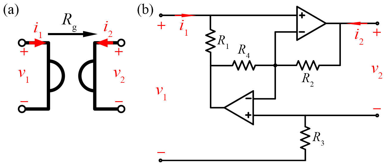
Figure 1: (a) Gyrator schematic and corresponding voltages, currents, and gyration resistance direction. (b) A possible circuit for gyrator implementation by using an opamp.

Consider the gyrator circuit shown in Fig. 1(b) implemented using two opamps and four resistors. By selecting the proper value for the resistors, we control the gyration resistance. In general, a gyrator is a nonreciprocal two-port network represented by an asymmetric impedance matrix $\underline{Z}$ as [31]

$$\mathbf{\underline{Z}}=\left[\begin{array}[]{cc}0&-R_{3}\\ \frac{R_{1}R_{2}}{R_{4}}&0\end{array}\right].$$ (2)

III EPD Condition in Series and Parallel Configuration

We show two configurations in which we get an EPD by using gyrator-based circuits. Indeed, series and parallel resonators are here utilized in two different configurations. Later on, we will write the required circuit equations in Liouvillian formalism. The eigenvalue problem is solved, leading to resonant frequencies, and the condition for obtaining EPD at the desired frequency is introduced. Finally, we show the perturbation effects on the circuit’s eigenfrequencies, and we verify our theoretical calculations by using a time domain circuit simulator (Keysight Advanced Design System (ADS)). Then, in order to provide a comprehensive analysis of the presented circuits, in Sections III-C and III-D, we account for losses in the resonators and we analyze the eigenfrequencies by perturbing the value of the resistances in each resonator.

III-A Series LC - Series LC

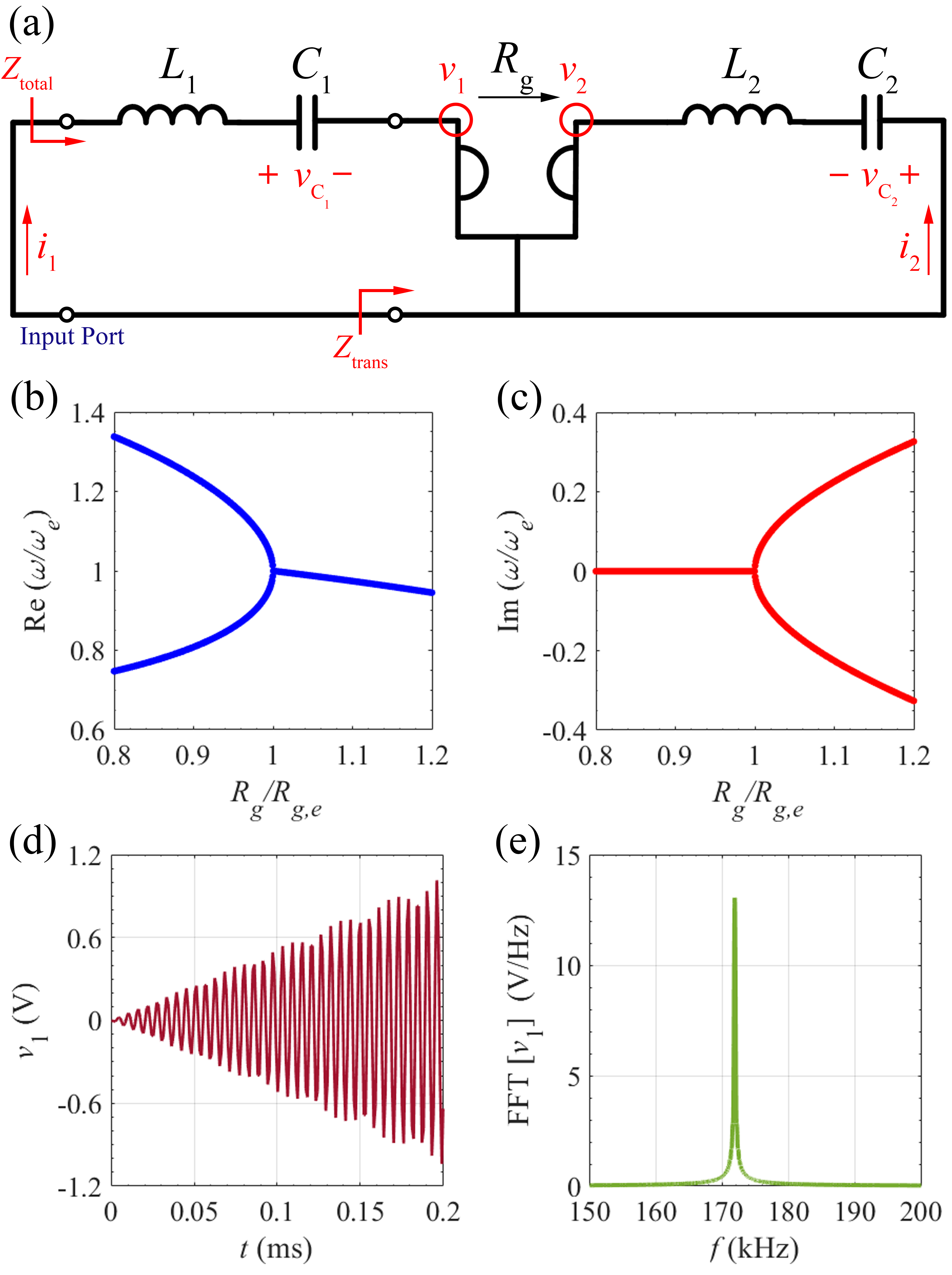
Figure 2: (a) Series-series configuration: two different LC resonators in series configuration connected via an ideal gyrator. The right resonator is made of negative inductance and capacitance. Variation of the (b) real and (c) imaginary parts of the two eigenfrequencies to a gyration resistance perturbation. The bifurcation in the real part is observed for $R_{g}<R_{ge}$. Voltage $v_{1}$ under the EPD condition in the (d) time domain, and (e) frequency domain. The result for the frequency domain is calculated from $150\mathrm{\>kHz}$ to $200\>\mathrm{kHz}$ with $10^{6}$ samples in the time window between $0\>\mathrm{ms}$ to $0.2\>\mathrm{ms}$.

In the first configuration, two series LC tanks are connected by a gyrator, as illustrated in Fig. 2(a). We assume that all components are ideal, and the circuit does not contain any resistance. By writing down the Kirchhoff voltage law equations in two loops, we obtain

$$\begin{cases}\ddot{Q}_{1}=-\frac{1}{C_{1}L_{1}}Q_{1}+\frac{R_{g}}{L_{1}}\dot{Q}_{2}\\ \ddot{Q}_{2}=-\frac{1}{C_{2}L_{2}}Q_{2}-\frac{R_{g}}{L_{2}}\dot{Q}_{1}\end{cases}$$ (3)

where $Q_{n}$ is the stored charge in the capacitor $C_{n}$ ($n=1$ for the left segment and $n=2$ for the right segment). In order to solve these equations, it is convenient to define a state vector as $\boldsymbol{\Psi}\equiv[Q_{1},Q_{2},\dot{Q}_{1},\dot{Q}_{2}]^{T}$, which consists of a combination of stored charges and their derivative (currents) on both sides, and the superscript $T$ denotes the transpose operation. Thus, in Liouvillian form, we write

$$\mathcal{\mathrm{\frac{d\boldsymbol{\Psi}}{dt}=\mathbf{\underline{M}}\boldsymbol{\Psi},\;\;}\mathbf{\underline{M}}}=\left(\begin{array}[]{cccc}0&0&1&0\\ 0&0&0&1\\ -\omega_{01}^{2}&0&0&\frac{R_{g}}{L_{1}}\\ 0&-\omega_{02}^{2}&-\frac{R_{g}}{L_{2}}&0\end{array}\right),$$ (4)

where $\underline{\mathbf{M}}$ is the $4\times 4$ circuit matrix. Furthermore, $\omega_{01}=1/\sqrt{C_{1}L_{1}}$, and $\omega_{02}=1/\sqrt{C_{2}L_{2}}$ are resonance angular frequencies of two isolated left and right circuits. Assuming signals of the form $Q_{n}\varpropto e^{j\omega t}$, we write the eigenvalue problem associated with the circuit equations, and the characteristic equation is obtained from $\det(\underline{\mathbf{M}}-j\omega\underline{\mathbf{I}})=0$, where $\underline{\mathbf{I}}$ is the identity matrix, leading to

$$\omega^{4}-\omega^{2}\left(\omega_{01}^{2}+\omega_{02}^{2}+\frac{R_{g}^{2}}{L_{1}L_{2}}\right)+\omega_{01}^{2}\omega_{02}^{2}=0.$$ (5)

In this characteristic equation, $\omega$ is an angular eigenfrequency of the system. All the $\omega$’s coefficients are real hence $\omega$ and $\omega^{*}$ are both roots of the characteristic equation, where * represents the complex conjugate operation. Moreover, it is a quadratic equation in $\omega^{2}$; therefore, $\omega$ and $-\omega$ are both solutions. In the following example, the two solutions with $\mathrm{Re}(\omega)>0$ are shown in Figs. 2(b) and (c). For $R_{g}=0$, the two resonators are uncoupled, and the two circuits have two angular eigenfrequency pairs of $\omega_{1,3}=\pm\omega_{01}$, and $\omega_{2,4}=\pm\omega_{02}$. We assume that each single resonator’s resonance frequency is real-valued; this happens when inductance and capacitance in the same resonator have both the same sign. In our case, component values on the left side are positive, whereas they are negative on the right side. We explain the reason for this issue in Appendix VI-A1. The angular eigenfrequencies (resonance frequencies) in the coupled circuit are calculated as

$$\omega_{1,3}=\pm\sqrt{a+b},\;\omega_{2,4}=\pm\sqrt{a-b},$$ (6)

where

$$a=\frac{1}{2}\left(\omega_{01}^{2}+\omega_{02}^{2}+\frac{R_{g}^{2}}{L_{1}L_{2}}\right),$$ (7)

$$\begin{array}[]{c}b^{2}=a^{2}-\omega_{01}^{2}\omega_{02}^{2}.\end{array}$$ (8)

According to Eq. (6), the EPD condition requires

$$b=0,$$ (9)

and the EPD angular frequency is $\omega_{e}=\pm\sqrt{a}$. Here we assume positive values for $a$ in order to have a real EPD angular frequency (and we will only refer to positive values of $\omega_{e}$ in the following). From Eq. (8), the EPD condition is rewritten as $a^{2}=\omega_{01}^{2}\omega_{02}^{2}.$ Since we look for real-valued EPD frequencies, $a>0$, and from Eq. 7 one has

$$\omega_{01}^{2}+\omega_{02}^{2}-\omega_{gs}^{2}>0,$$ (10)

where it has been convenient to define the equivalent gyrator frequency $\omega_{gs}^{2}=-R_{g}^{2}/(L_{1}L_{2})$ for the series-series configuration (note that $\omega_{gs}^{2}>0$ because one inductor is negative). Finally, the EPD frequency is calculated by using Eqs. (7), (8), and (9) as

$$\begin{array}[]{c}\omega_{e}=\sqrt{\frac{1}{2}\left(\omega_{01}^{2}+\omega_{02}^{2}-\omega_{gs}^{2}\right)}=\sqrt{\omega_{01}\omega_{02}}.\end{array}$$ (11)

Without loss of generality, we explain the required procedure to obtain an EPD in this configuration by presenting a specific example. Many different combinations of values for the circuit’s components will satisfy the EPD condition, and here as an example, we assume this set of values for components: $L_{1}=47\mathrm{\>\mu H}$, $L_{2}=-47\mathrm{\>\mu H}$, $C_{2}=-47\mathrm{\>nF}$, and $R_{g}=50\>\Omega$. As mentioned before, the desired value for the gyration resistance is achieved by determining the appropriate values for the resistors in the circuit for the gyrator illustrated in Fig. 1(b). Finally, the capacitance $C_{1}$ is determined by solving the quadratic equation from the EPD condition in Eq. (9). There are two different values of the capacitance $C_{1}$ in the first resonator that satisfy Eq. (9), namely $C_{1,e}=7.05\>\mathrm{nF}$ and $C_{1,e}=139.16\>\mathrm{nF}$. For the smaller value ($C_{1,e}=7.05\>\mathrm{nF}$), we obtain a positive result for $a$ in Eq. (10), so the EPD frequency is real. On the contrary, the second value $(C_{1,e}=139.16\>\mathrm{nF})$ gives us a negative result for $a$, so the EPD frequency would be imaginary and we discard it since we investigate gyrator-based circuits with real-valued EPD frequency in this paper. In the following, we selected the smaller value for the capacitance of the left resonator, $C_{1}=7.05\>\mathrm{nF}$. The results in Figs. 2(b) and (c) exhibit the two branches of the real and imaginary parts of perturbed eigenfrequencies obtained from the eigenvalue problem, varying the gyrator resistance $R_{g}$ in the neighborhood of $R_{g,e}=50\>\Omega$. In this example, we obtain $\omega_{e}=1.08\times 10^{6}\>\mathrm{rad/s}$ and the coalesced eigenvalues at EPD are exceedingly sensitive to perturbations in system parameters.

The time domain simulation results obtained using the Keysight ADS circuit simulator are illustrated in Figs. 2(d) and (e), they show the voltage $v_{1}(t)$ in the left resonator, and its spectrum, where we put $1\>\mathrm{mV}$ as an initial voltage on $C_{1}$. In the circuit simulator, an ideal gyrator has been utilized. According to Fig. 2(d), the voltage grows linearly with increasing time. This important aspect is peculiar of an EPD, and it is the result of coalescing system eigenvalues and eigenvectors that also corresponds to a double pole in the system. A linear growth indicates a second-order EPD in the system. We take a fast Fourier transform (FFT) of the voltage $v_{1}(t)$ to show the frequency spectrum, and the calculated result is illustrated in Fig. 2(e). The observed oscillation frequency is $f_{o}=172.05\mathrm{\>kHz}$, which is in good agreement with the theoretical value $\omega_{e}/(2\pi)$ calculated above.

By perturbing the gyration resistance, the operation point moves away from the EPD. By selecting a lower value for the gyration resistance, the system has two different real-valued eigenfrequencies. For instance, we reduce the amount of perturbed parameter by $5\%$ equal to $R_{g}=47.5\>\Omega<R_{g,e}=50\>\Omega$. In the perturbed condition, we do not observe any signal growth in the system with increasing time. If we consider an additive $5\%$ of perturbation in the gyration resistance, i.e., $R_{g}=52.5\>\Omega$ >$R_{g,e}=50\>\Omega$, the imaginary part of the angular eigenfrequencies is non-zero, and it causes eigensolutions with damping and growing signals in the system. Since the signal is in the form of $Q_{n}\varpropto e^{j\omega t}$, the eigenfrequency with negative imaginary part is associated to an exponentially growing signal.

III-B Parallel LC - Parallel LC

In the second configuration, two parallel LC tanks are coupled by a gyrator as displayed in Fig. 3(a). Similarly to what was discussed for the series-series configuration, we find the EPD condition in this circuit by writing the Kirchhoff current law equations and finding the Liouvillian matrix. Hence, by expressing current and voltages in terms of charges, the following equations are to be satisfied

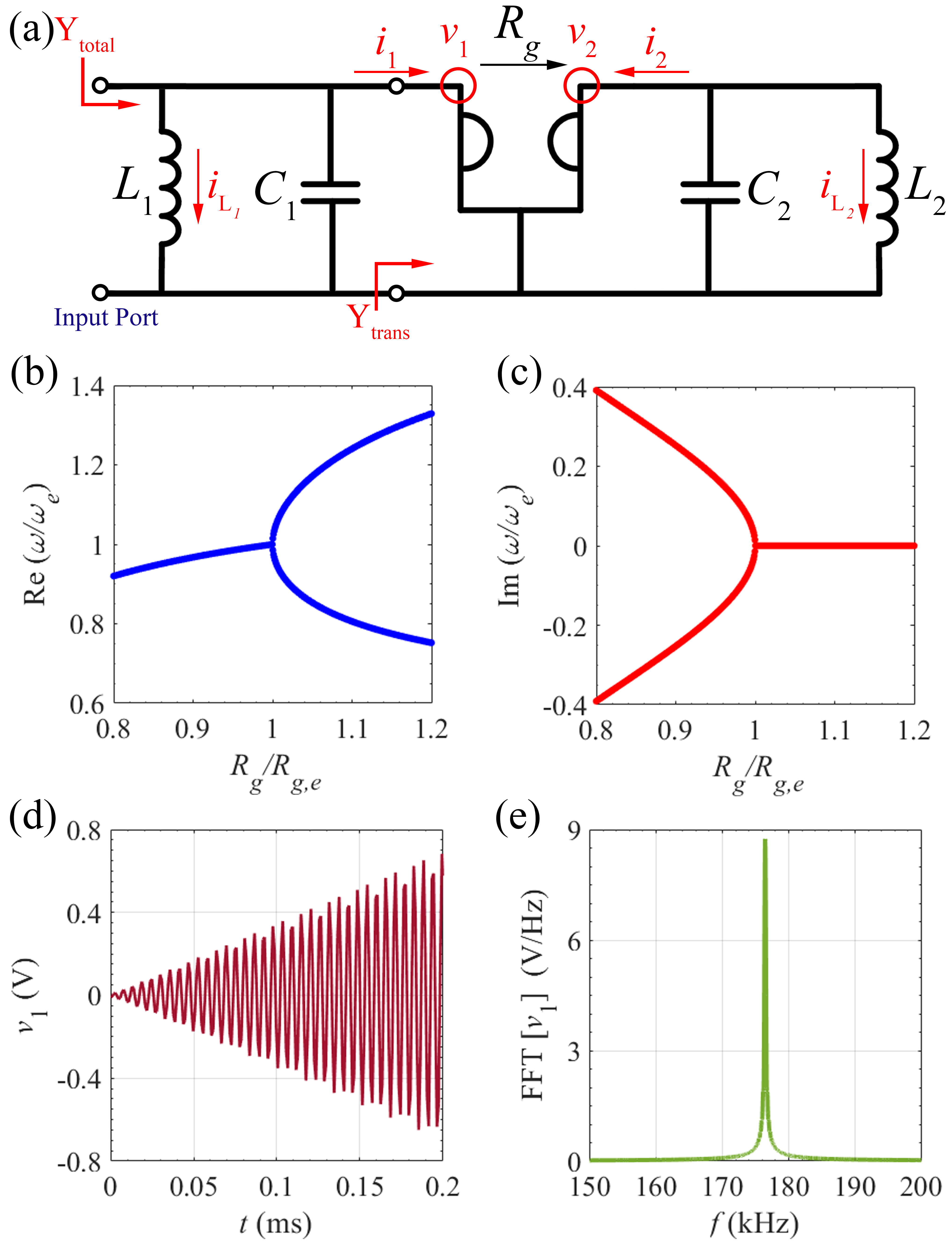
Figure 3: (a) Parallel-parallel configuration: two different LC resonators in parallel configuration connected via an ideal gyrator. The right resonator is made of negative inductance and capacitance. Variation of the (b) real and (c) imaginary parts of the two eigenfrequencies to a gyration resistance perturbation. The bifurcation in the real part is observed for $R_{g}>R_{ge}$. Voltage $v_{1}$ under the EPD condition in the (d) time domain, and (e) frequency domain. The result for the frequency domain is calculated from $150\mathrm{\>kHz}$ to $200\>\mathrm{kHz}$ with $10^{6}$ samples in the time window between $0\>\mathrm{ms}$ to $0.2\>\mathrm{ms}$.

$$\begin{cases}\ddot{Q}_{1}=-\frac{1}{C_{1}L_{1}}Q_{1}+\frac{1}{R_{g}C_{2}}\dot{Q}_{2}\\ \ddot{Q}_{2}=-\frac{1}{C_{2}L_{2}}Q_{2}-\frac{1}{R_{g}C_{1}}\dot{Q}_{1}\end{cases}$$ (12)

By using the state vector $\boldsymbol{\Psi}\equiv[Q_{1},Q_{2},\dot{Q}_{1},\dot{Q}_{2}]^{T}$ analogously to what was described in the series-series configuration, leads to the Liouvillian representation

$$\mathcal{\mathrm{\frac{d\boldsymbol{\Psi}}{dt}=\mathbf{\underline{M}}\boldsymbol{\Psi},\;\;}\mathbf{\underline{M}}}=\left(\begin{array}[]{cccc}0&0&1&0\\ 0&0&0&1\\ -\omega_{01}^{2}&0&0&\frac{1}{R_{g}C_{2}}\\ 0&-\omega_{02}^{2}&-\frac{1}{R_{g}C_{1}}&0\end{array}\right).$$ (13)

The eigenfrequencies of the circuit are calculated by solving the associated characteristic equation

$$\omega^{4}-\omega^{2}\left(\omega_{01}^{2}+\omega_{02}^{2}+\frac{1}{C_{1}C_{2}R_{g}^{2}}\right)+\omega_{01}^{2}\omega_{02}^{2}=0.$$ (14)

As for the series-series case, all the $\omega$’s coefficients are real hence $\omega$ and $\omega^{*}$ are both roots of the characteristic equation. Moreover, it is a quadratic equation in $\omega^{2}$, therefore $\omega$ and $-\omega$ are both solutions. In the following example, the two solutions with $\mathrm{Re}(\omega)>0$ are shown in Figs. 3(b) and (c). The system’s angular eigenfrequencies are

$$\omega_{1,3}=\pm\sqrt{a+b},\;\omega_{2,4}=\pm\sqrt{a-b},$$ (15)

$$a=\frac{1}{2}\left(\omega_{01}^{2}+\omega_{02}^{2}+\frac{1}{C_{1}C_{2}R_{g}^{2}}\right),$$ (16)

$$\begin{array}[]{c}b^{2}=a^{2}-\omega_{01}^{2}\omega_{02}^{2}.\end{array}$$ (17)

The EPD is obtained when the parallel circuit’s resonance frequencies coalesce, i.e., when

$$b=0.$$ (18)

According to Eq. (17), the required condition for EPD is $a^{2}=\omega_{01}^{2}\omega_{02}^{2}$. The EPD angular frequency is then given by $\omega_{e}=\pm\sqrt{a}$, and we assume $a>0$ to have a real EPD angular frequency. The condition to obtain real value for EPD frequency is rewritten as

$$\omega_{01}^{2}+\omega_{02}^{2}-\omega_{gp}^{2}>0,$$ (19)

where it has been convenient to define $\omega_{gp}^{2}=-1/(C_{1}C_{2}R_{g}^{2})$ for the parallel-parallel configuration (note that $\omega_{gp}^{2}>0$ because one capacitor is negative) for the parallel configuration. When both Eqs. (18) and (19) are satisfied, two eigenfrequencies coalesce at a real EPD angular frequency

$$\begin{array}[]{c}\omega_{e}=\sqrt{\frac{1}{2}\left(\omega_{01}^{2}+\omega_{02}^{2}-\omega_{gp}^{2}\right)}=\sqrt{\omega_{01}\omega_{02}}.\end{array}$$ (20)

As an example, we use the following values: $L_{1}=47\mathrm{\>\mu H}$, $L_{2}=-47\mathrm{\>\mu H}$, $C_{2}=-47\mathrm{\>nF}$, and $R_{g}=50\>\Omega$. As already mentioned in the series-series configuration, by imposing Eq. (18) to be satisfied, we obtain two values of capacitance $C_{1,e}=6.34\>\mathrm{nF}$ and $C_{1,e}=125.25\>\mathrm{nF}$. In this parallel case, both capacitors lead to $a>0$, enabling the EPD angular frequency to be real valued. Indeed, the $C_{1,e}=6.34\>\mathrm{nF}$ leads to $\omega_{e}=1.11\times 10^{6}\>\mathrm{rad/s}$, whereas $C_{1,e}=125.25\>\mathrm{nF}$ leads to $\omega_{e}=5.26\times 10^{5}\>\mathrm{rad/s}$. In the following we use $C_{1,e}=6.34\>\mathrm{nF}$. The results in Figs. 3(b) and (c) show the branches of the real and imaginary parts of perturbed eigenfrequencies obtained from the eigenvalue problem when varying the gyrator resistance near $R_{g,e}=50\>\Omega$. The bifurcation of the real part in this case happens for $R_{g}>R_{g,e}$ , whereas for the series-series case it happened for $R_{g}<R_{g,e}$. Perturbing other components like $C_{1}$ or $L_{1}$ leads to analogous results.

The time domain simulation result for the node voltage $v_{1}$ in Fig. 3(d) is obtained using the Keysight ADS circuit simulator by employing the ideal model for the gyrator. We have assumed the capacitor has an initial voltage on $C_{1}$ equal to $1\>\mathrm{mV}$. The voltage grows linearly by increasing time, demonstrating two circuit eigenvalues are coalescing, and the system exhibits a double pole. This is peculiar of a second-order EPD. The spectrum of the voltage $v_{1}$ is calculated by imposing the FFT. According to Fig. 3(e), the oscillation frequency is $f_{o}=176.66\mathrm{\>kHz}$, which is in good agreement with the theoretical value $\omega_{e}/(2\pi)$ calculated above.

By perturbing the gyration resistance, the circuit does not operate at the EPD anymore. For a higher gyration resistance value, $R_{g}=52.5\>\Omega>R_{g,e}=50\>\Omega$ as a $5\%$ increase, we obtain two distinct real-valued eigenfrequencies in the system. Thus, we could estimate the amount of perturbation in $R_{g}$ by measuring the frequency of these two resonances. On the other hand, by reducing the amount of perturbed parameter by $5\%$, leading to $R_{g}=47.5\>\Omega<R_{g,e}=50\>\Omega$, the system has two complex eigenfrequencies with non-zero imaginary parts. The circuit contains signals that are both damping or growing exponentially. It is worth mentioning that the presented series-series and parallel-parallel configuration are dual to each other, as discussed in Appendix VI-C.

III-C Series RLC - Series RLC

In the following section, we analyze the EPD condition in the series-series configuration by accounting for series resistors $R_{1}$ and $R_{2}$ in both resonators. Using the Liouvillian formalism, the Kirchhoff voltage law equations for the two loops of the circuit in Fig. 4(a), and the same state vector as before, $\boldsymbol{\Psi}\equiv[Q_{1},Q_{2},\dot{Q}_{1},\dot{Q}_{2}]^{T}$, we obtain

$$\mathcal{\mathrm{\frac{d\boldsymbol{\Psi}}{dt}=\mathbf{\underline{M}}\boldsymbol{\Psi},\;\;}\mathbf{\underline{M}}}=\left(\begin{array}[]{cccc}0&0&1&0\\ 0&0&0&1\\ -\omega_{01}^{2}&0&-\gamma_{1}&\frac{R_{g}}{L_{1}}\\ 0&-\omega_{02}^{2}&-\frac{R_{g}}{L_{2}}&-\gamma_{2}\end{array}\right),$$ (21)

where, $\gamma_{1}=R_{1}/L_{1}$, and $\gamma_{2}=R_{2}/L_{2}$ describe losses (losses on the right circuit are represented by a negative $\gamma_{2}$ since $L_{2}$ is negative). Signals in such a circuit are proportional to $e^{j\omega t}$ where $\omega$ is an eigenfrequency. These eigenfrequencies are solutions to the following characteristic equation

$$\begin{array}[]{c}\omega^{4}-j\omega^{3}\left(\gamma_{1}-\gamma_{2}\right)-\omega^{2}\left(\omega_{01}^{2}+\omega_{02}^{2}+\gamma_{1}\gamma_{2}+\frac{R_{g}^{2}}{L_{1}L_{2}}\right)\\ +j\omega\left(\gamma_{1}\omega_{02}^{2}+\gamma_{2}\omega_{01}^{2}\right)+\omega_{01}^{2}\omega_{02}^{2}=0.\end{array}$$ (22)

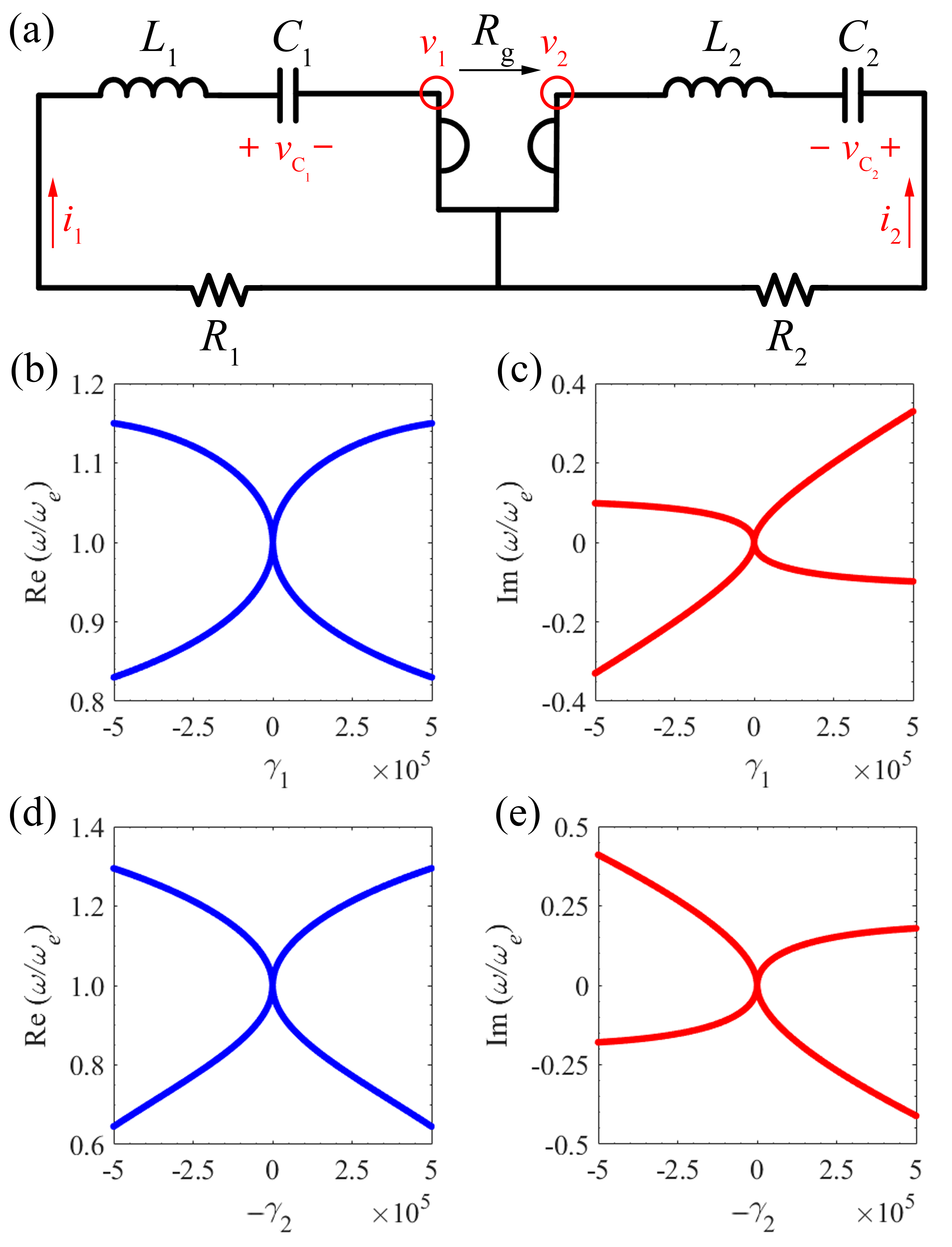
Figure 4: (a) Schematic view of series-series configuration including a resistor in each resonator. Variation of (b) real and (c) imaginary parts of the angular eigenfrequencies to a resistor perturbation on the left side; in this figure, $\gamma_{1}$ is varied whereas we assumed $\gamma_{2}=0$. Variation of (d) real and (e) imaginary parts of the angular eigenfrequencies to a resistor perturbation on the right side; in this figure, $-\gamma_{2}$ is varied whereas we assumed $\gamma_{1}=0$.

An eigenfrequency with a negative imaginary part is associated with an exponentially growing signal. The coefficients of the odd-power terms of the angular eigenfrequency ($\omega$ and $\omega^{3}$) in the characteristic equation Eq. (22) are imaginary. In the characteristic equation, eigenfrequencies $\omega$ and $-\omega^{*}$ are both roots. In order to have a stable circuit with real-valued eigenfrequencies the odd-power terms of the angular eigenfrequency $-j\omega^{3}(\gamma_{1}-\gamma_{2})$ and $j\omega(\gamma_{1}\omega_{02}^{2}+\gamma_{2}\omega_{01}^{2})$ in the characteristic equation Eq. (22) should be zero, otherwise a complex eigenfrequency needed to satisfy the characteristic equation Eq. (22). The coefficient of the $\omega^{3}$ term is zero when $\gamma_{1}=\gamma_{2}$, and under this condition the coefficient of the $\omega$ term $\gamma_{1}\left(\omega_{02}^{2}+\omega_{01}^{2}\right)$ is non-zero value because $\omega_{01}^{2}$ and $\omega_{02}^{2}$ are both positive. Moreover, the coefficient of the $\omega$ term vanishes when $\gamma_{1}/\gamma_{2}=-\omega_{01}^{2}/\omega_{02}^{2}$, and under this condition, the coefficient of the $\omega^{3}$ term $\gamma_{1}\left(1+\omega_{02}^{2}/\omega_{01}^{2}\right)$ cannot vanish. Thus, it is not possible to have all real-valued coefficients in the characteristic polynomials, unless $\gamma_{1}=\gamma_{2}=0$ which corresponds to a lossless circuit.

In Figs. 4(b) and (c), $\gamma_{1}$ is varied while we assume $\gamma_{2}=0$. In Figs. 4(d) and (e), $-\gamma_{2}$ is perturbed while $\gamma_{1}=0$. These two figures show the real and imaginary parts of eigenfrequencies when we perturb each resistor individually. In these examples, we have used the same values for the circuit components as used earlier in the lossless series-series configuration. The EPD angular frequency is obtained when $\gamma_{1}=\gamma_{2}=0$, which is the same EPD frequency of the lossless configuration shown in Section III-A. In Figs. 4(b-e), we observe the bifurcations of the real and imaginary parts of the eigenfrequencies, so the circuit is very sensitive to variations in both resistance values. Angular eigenfrequencies here are complex-valued; it means that by perturbing $\gamma_{1}$ or $\gamma_{2}$ away from $\gamma_{1}=\gamma_{2}=0$, the circuit gets unstable; hence it starts to oscillate with the fundamental frequency associated with the real part of the unstable angular eigenfrequency. When $\gamma_{1}$ or $\gamma_{2}$ is perturbed from the EPD value, the oscillation frequency is shifted from the EPD frequency, and it could be measured for sensing applications. In Figs. 4(b-e), both conditions $\gamma_{1}>0$ and $-\gamma_{2}>0$ represent losses, whereas the conditions $\gamma_{1}<0$ and $-\gamma_{2}<0$ represent gains in the circuit through a negative resistance. In any case, by adding either losses or gains, the system is unstable. We observe more sensitivity when perturbing the resistor $R_{2}$, on the right side, because a small perturbation in resistance value results in a larger variation of the eigenfrequencies than when varying $R_{1}$. Indeed, a wider bifurcation indicates a higher sensitivity. In order to compensate instability effect of the losses in the circuit, an independent series gain could be added to each resonator, but this is not pursued in this paper.

III-D Parallel RLC - Parallel RLC

By using the same approach presented in the previous section, we now consider parallel resistors on both sides of the parallel-parallel circuit configuration, as in 5(a). We write the two Kirchhoff current law equations and by using the same state vector introduced in a lossless parallel-parallel configuration, $\boldsymbol{\Psi}\equiv[Q_{1},Q_{2},\dot{Q}_{1},\dot{Q}_{2}]^{T}$, the circuit dynamics are described using the Liouvillian formalism as

$$\mathcal{\mathrm{\frac{d\boldsymbol{\Psi}}{dt}=\mathbf{\underline{M}}\boldsymbol{\Psi},\;\;}\mathbf{\underline{M}}}=\left(\begin{array}[]{cccc}0&0&1&0\\ 0&0&0&1\\ -\omega_{01}^{2}&0&-\gamma_{1}&\frac{1}{R_{g}C_{2}}\\ 0&-\omega_{02}^{2}&-\frac{1}{R_{g}C_{1}}&-\gamma_{2}\end{array}\right).$$ (23)

Here, $\gamma_{1}=1/(R_{1}C_{1})$ and $\gamma_{2}=1/(R_{2}C_{2})$ represent the resistors’ losses (losses on the right circuit are represented by a negative $\gamma_{2}$ since $C_{2}$ is negative). Similarly to the lossless parallel-parallel configuration, the eigenfrequencies are found by solving the characteristic equation

$$\begin{array}[]{c}\omega^{4}-j\omega^{3}\left(\gamma_{1}-\gamma_{2}\right)-\omega^{2}\left(\omega_{01}^{2}+\omega_{02}^{2}+\gamma_{1}\gamma_{2}+\frac{1}{R_{g}^{2}C_{1}C_{2}}\right)\\ +j\omega\left(\gamma_{1}\omega_{02}^{2}+\gamma_{2}\omega_{01}^{2}\right)+\omega_{01}^{2}\omega_{02}^{2}=0.\end{array}$$ (24)

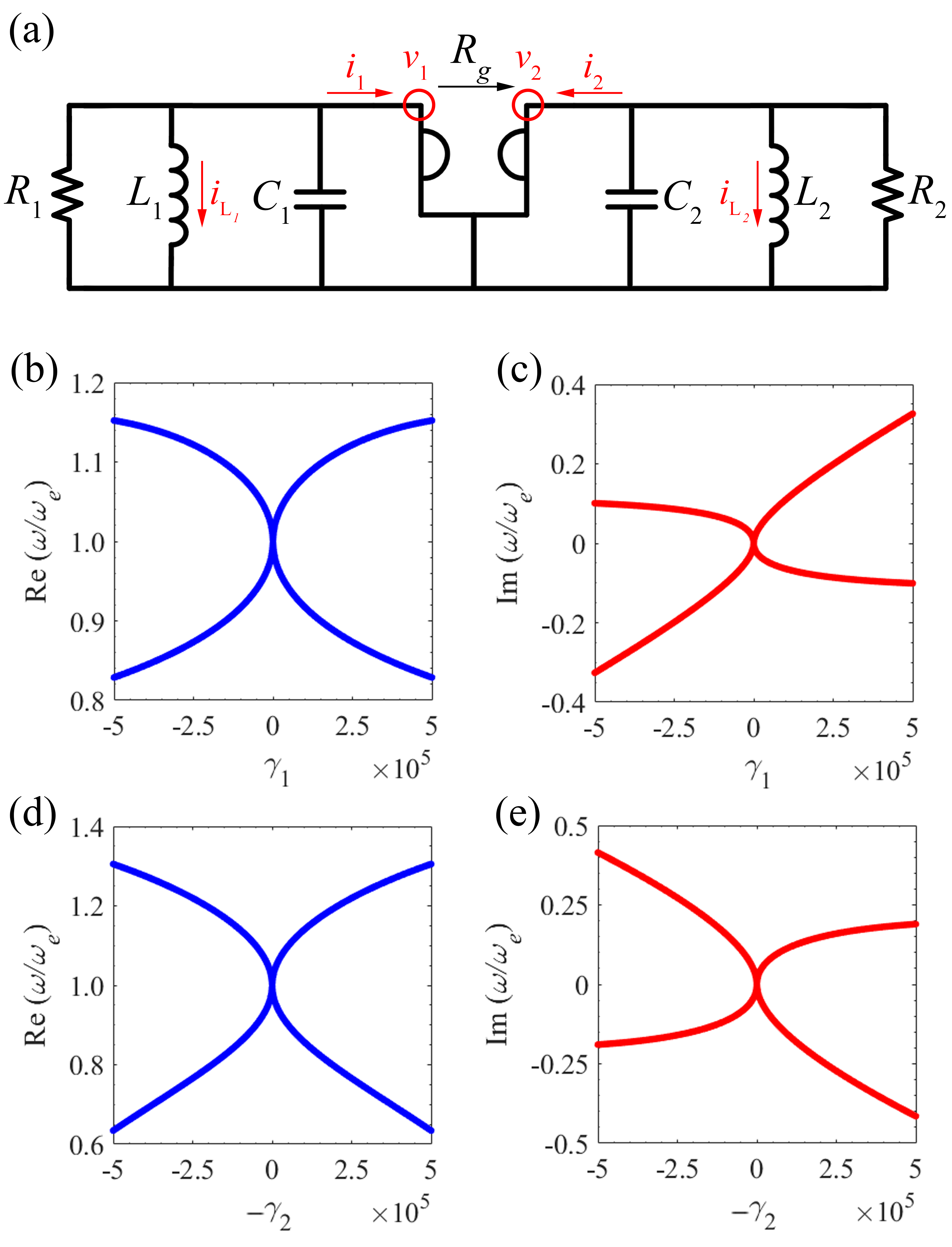
Figure 5: (a) Schematic view of parallel-parallel configuration including a resistor in each resonator. Variation of (b) real and (c) imaginary part of the angular eigenfrequencies to a resistor perturbation on the left side; in this figure, $\gamma_{1}$ is varied whereas we assumed $\gamma_{2}=0$. Variation of (d) real and (e) imaginary part of the angular eigenfrequencies to a resistor perturbation on the right side; in this figure, $-\gamma_{2}$ is varied whereas we assumed $\gamma_{1}=0$.

Also in this case, the coefficients of the odd-power terms of the angular eigenfrequency ($\omega$ and $\omega^{3}$) in the characteristic equation Eq. (24) are imaginary. In the characteristic equation, eigenfrequencies $\omega$ and $-\omega^{*}$ are both roots. In order to have a stable circuit with real-valued eigenfrequencies the odd-power terms of the angular eigenfrequency $-j\omega^{3}(\gamma_{1}-\gamma_{2})$ and $j\omega(\gamma_{1}\omega_{02}^{2}+\gamma_{2}\omega_{01}^{2})$ in the characteristic equation Eq. (24) should be zero. Otherwise a complex eigenfrequency needed to satisfy the characteristic equation Eq. (24). The coefficient of the $\omega^{3}$ term is zero when $\gamma_{1}=\gamma_{2}$, and under this condition the coefficient of the $\omega$ term $\gamma_{1}\left(\omega_{02}^{2}+\omega_{01}^{2}\right)$ is non-zero value because $\omega_{01}^{2}$ and $\omega_{02}^{2}$ are both positive. Moreover, the coefficient of the $\omega$ term vanishes when $\gamma_{1}/\gamma_{2}=-\omega_{01}^{2}/\omega_{02}^{2}$, and under this condition, the coefficient of the $\omega^{3}$ term $\gamma_{1}\left(1+\omega_{02}^{2}/\omega_{01}^{2}\right)$ cannot vanish. Thus, it is not possible to have all real-valued coefficients in the characteristic polynomials, unless $\gamma_{1}=\gamma_{2}=0$, which corresponds to a lossless circuit. There is no condition to make both $\omega$ and $\omega^{3}$ coefficients equal to zero hence eigenfrequencies are complex leading to instabilities that cause oscillations.

In Figs. 5(b) and (c), we vary $\gamma_{1}$ and assumed $\gamma_{2}=0$, whereas in Figs. 5(d) and (e), we perturbed $-\gamma_{2}$ and assumed $\gamma_{1}=0$. When $\gamma_{1}=\gamma_{2}=0$, the EPD frequency is the same as the one found earlier for the lossless configuration in Section III-B. Figs. 5 (b)-(e) show the bifurcation of the real and imaginary parts of eigenfrequencies on both sides of the EPD. It means that the circuit is very sensitive to both positive and negative variations in the resistance value. The angular eigenfrequencies are complex-valued for any amount of losses, and the circuit is in the self-oscillation regime. The circuit’s signal oscillates with the frequency associated with the real part of the unstable eigenfrequency, and the signal is exponentially growing based on the unstable imaginary part of the eigenfrequency. The calculated results show that we achieve higher sensitivity when perturbing $\gamma_{2}$. In order to compensate instability effect of the losses in the circuit, an independent parallel gain could be added to each resonator, but this is not pursued here.

IV Parallel Circuit Sensitivity

The eigenvalues (resonance frequencies) at EPDs are exceedingly sensitive to perturbations of parameters of the system. Here, we show that the sensitivity of a system’s observable to a specific variation of a component’s value is large because of the EPD. Let us consider the parallel circuit in the EPD regime, with the values of the components given in Section III-B. We select the parallel case because all elements are grounded and this sometimes represents a simplification when using realistic active components that require biasing. For simplicity, we discuss the case without resistances and we define the relative circuit perturbation $\Delta_{\mathrm{X}}$ as

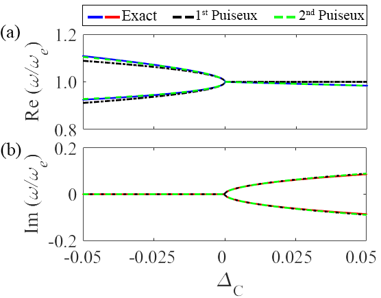
Figure 6: High sensitivity of the (a) real and (b) imaginary parts of the eigenfrequencies to relative capacitance perturbation $\Delta_{\mathrm{C}}=(C_{\mathrm{1}}-C_{\mathrm{1,e}})/C_{\mathrm{1,e}}$. The two perturbed frequencies are real for $\Delta_{\mathrm{C}}<0$.

$$\Delta_{\mathrm{X}}=\frac{X-X_{\mathrm{e}}}{X_{\mathrm{e}}},$$ (25)

where $X$ is the perturbated value of a component, and $X_{\mathrm{e}}$ is the unperturbed value that provides the EPD. The subscript “X” denotes the perturbed parameter. In this section, we consider variations of $C_{\mathrm{1}}$, and $L_{\mathrm{1}}$, one at a time, in the parallel configuration. The calculated diagram for the real and imaginary parts of the eigenfrequencies near the EPD are shown in Figs. 6 and 7. We conclude that the individual variation of the parameters of $C_{\mathrm{1}}$, or $L_{\mathrm{1}}$ show similar sensitivity behavior, i.e., the real part of the eigenfrequencies splits for $\Delta_{\mathrm{X}}<0$. Note that the $L_{\mathrm{1}}$ perturbation shows higher sensitivity because of the wider bifurcation in the dispersion diagram.

We explain the extreme sensitivity by resorting to the general theory of EPDs. Note that a perturbation in $\Delta_{\mathrm{X}}$ value leads to a perturbed matrix $\mathbf{\underline{M}}(\Delta_{\mathrm{X}})$. Consequently, the two degenerate eigenvalues occurring at the EPD change considerably due to the small perturbation in $\Delta_{\mathrm{X}}$, resulting in two distinct eigenfrequencies $\omega_{\mathrm{\mathit{p}}}(\Delta_{\mathrm{X}})$, with $p=1,2$. The two perturbed eigenvalues near an EPD are represented by a single convergent Puiseux series (also called fractional power expansion), where the coefficients are calculated using the explicit recursive formulas given in [32]. An approximation of $\omega_{p}(\Delta_{\mathrm{X}})$ around a second-order EPD is given by

$$\omega_{p}(\Delta_{\mathrm{X}})\approx\omega_{e}+(-1)^{p}\alpha_{1}\sqrt{\Delta_{\mathrm{X}}}+\alpha_{2}\Delta_{\mathrm{X}}.$$ (26)

Following [32], we calculate the coefficients as

$$\alpha_{1}=\sqrt{-\frac{\frac{\partial H(\Delta_{\mathrm{X}},\omega)}{\partial\Delta_{\mathrm{X}}}}{\frac{1}{2!}\frac{\partial^{2}H(\Delta_{\mathrm{X}},\omega)}{\partial\omega^{2}}}},$$ (27)

$$\alpha_{2}=-\frac{\alpha_{1}^{3}\frac{1}{3!}\frac{\partial^{3}H(\Delta_{\mathrm{X}},\omega)}{\partial\omega^{3}}+\alpha_{1}\frac{\partial^{2}H(\Delta_{\mathrm{X}},\omega)}{\partial\omega\partial\Delta_{\mathrm{X}}}}{\alpha_{1}\frac{\partial^{2}H(\Delta_{\mathrm{X}},\omega)}{\partial\omega^{2}}},$$ (28)

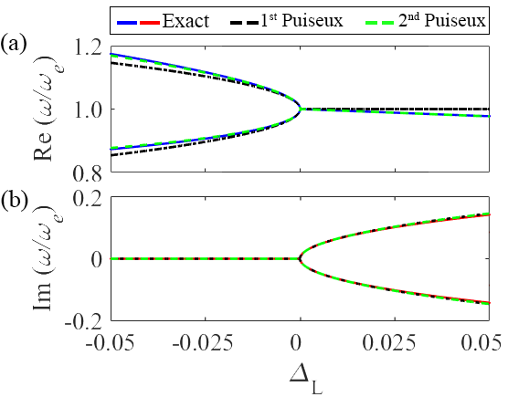
Figure 7: High sensitivity of the (a) real and (b) imaginary parts of the eigenfrequencies to relative inductance perturbation $\Delta_{\mathrm{L}}=(L_{\mathrm{1}}-L_{\mathrm{1,e}})/L_{\mathrm{1,e}}$. The two perturbed frequencies are real for $\Delta_{\mathrm{L}}<0$.

evaluated at the EPD, i.e., at $\Delta_{\mathrm{X}}=0$ and $\omega=\omega_{\mathrm{e}}$, where $H(\Delta_{\mathrm{X}},\omega)=\mathrm{det}[\mathbf{\underline{M}}(\Delta_{\mathrm{X}})-j\omega\underline{\mathbf{I}}]$. Eq. (26) indicates that for a small perturbation $\Delta_{\mathrm{X}}\ll 1,$ the eigenvalues change dramatically from their original degenerate value due to the square root function. In the first example, the perturbed parameter is the capacitance on the left circuit, $\Delta_{\mathrm{C}}=(C_{\mathrm{1}}-C_{\mathrm{1,e}})/C_{\mathrm{1,e}}$, and the Puiseux series first-order coefficient is calculated by Eq. (35) as $\alpha_{1}=j4.4138\times 10^{5}\>\mathrm{rad/s}$ and the second-order coefficient is calculated as $\alpha_{2}=-3.6503\times 10^{5}\>\mathrm{rad/s}$. The result in Fig. 6 shows the two branches of the perturbed eigenfrequencies $\omega$ obtained directly from the eigenvalue problem (i.e., from the dispersion equation) when the perturbation $\Delta_{\mathrm{C}}$ is applied. In this example, we consider $C_{1}$ as a sensing capacitance to detect possible variation in physical or chemical parameters transformed into electrical parameters (variation in other components could also be used in other different realistic scenarios). Fig. 6 explains that such perturbed eigenvalues can be estimated with excellent accuracy by employing the Puiseux series truncated at its second order (green dashed lines). We have also shown the first-order approximation in Fig. 6 for better comparison (black dashed lines), which is also in good agreement with the eigenfrequencies obtained by the dispersion equation. For a small positive value of $\Delta_{\mathrm{C}}$, the imaginary parts of the eigenfrequencies experience a sharp change, while their real parts remain more or less constant. A small negative value of $\Delta_{\mathrm{C}}$ causes a rapid variation in the real part of the eigenfrequencies.

In the second example, the perturbed parameter is the inductance on the left circuit, $\Delta_{\mathrm{L}}=(L_{\mathrm{1}}-L_{\mathrm{1,e}})/L_{\mathrm{1,e}}$, and the Puiseux series first-order coefficient is calculated by Eq. (36) as $\alpha_{1}=j7.2792\times 10^{5}\>\mathrm{rad/s}$ and the second-order coefficient is calculated as $\alpha_{2}=-5.1598\times 10^{5}\>\mathrm{rad/s}$. The calculated results in Fig. 7 show the two branches of the perturbed eigenfrequencies obtained from the eigenvalue problem (i.e., from the dispersion equation) when the perturbation in inductance is applied. This result shows that the perturbed eigenfrequencies can be estimated with high accuracy by applying the Puiseux series truncated at its second order. However, the first order already provides relatively accurate results. For a tiny value of positive perturbation, the imaginary parts of the eigenfrequencies undergo a sharp change, while their real parts remain more or less unchanged. A small negative amount of perturbation in the inductor value causes a rapid variation in the eigenfrequencies’ real part. This feature is one of the most extraordinary physical properties associated with the EPD concept, and it can be exploited for designing ultra-sensitive sensors [33].

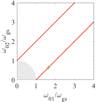
Figure 8: Possible combinations of $\omega_{01}$ and $\omega_{02}$ to have a real eigenfrequency in the series-series configuration are shown by the white area, and the gray area represents complex eigenfrequencies based on Eq. (10). Red curves satisfy Eq. (29) and show possible combinations of $\omega_{01}$ and $\omega_{02}$ that lead to a real EPD frequency. In these results, we kept $R_{g}$, $L_{1}$ and $L_{2}$ fixed as in Section III-A, and $C_{1}$ and $C_{2}$ are varied.

V Conclusions

We have shown that two resonators connected via a gyrator support an EPD when one resonator is made of a negative inductance and a negative capacitance. We have provided the theoretical conditions for such EPD to exist with a purely real frequency and we have verified our theoretical calculations by using a time domain circuit simulator (Keysight ADS). We have demonstrated that the eigenfrequencies are exceptionally sensitive to a perturbation of the system and this may have significant implications in ultra-sensitive sensing technology and RF sensors. A perturbation of the gyration resistance, capacitance or inductance leads to two real-valued shifted frequencies. The perturbation of the system can be estimated by measuring the changes in these two resonance frequencies. Moreover, adding a resistor on either side of the circuit leads to two complex eigenfrequencies for any small resistance value, implying that this circuit is unstable. Also, this latter property can be exploited to devise sensor schemes based on driving the system into oscillations. We believe that the shown results pave the way for possible new operation schemes for boosting the overall performance of ultra-high sensitive sensors.

VI Appendix

VI-A Components sign and simplification of EPD condition

VI-A1 Series-Series Configuration

In order to obtain an EPD in the series-series configuration using Eqs. (7), (8) and (9) the following equation must be satisfied:

$$\left(\omega_{01}-\omega_{02}\right)^{2}=\omega_{gs}^{2}.$$ (29)

We investigate three possible scenarios to satisfy Eq. (29). First, if $\omega_{01}$ and $\omega_{02}$ are pure real, the value of $L_{1}$ or $L_{2}$ should be negative to have the same sign on both sides of Eq. (29). Thus, one of the resonators should have a negative inductance to have a pure real $\omega_{01}$ or $\omega_{02}$. Second, if both $\omega_{01}$ and $\omega_{02}$ have imaginary values, the considered values for $L_{1}$ and $L_{2}$ should have the same sign, either positive or negative. When $L_{1}$ and $L_{2}$ are positive, $C_{1}$ and $C_{2}$ should be negative or vice versa. Finally, if just one of the $\omega_{01}$ or $\omega_{02}$ is imaginary and the other one has a real value, there are no conditions to obtain an EPD.

To have a real EPD frequency $\omega_{e}=\pm\sqrt{a}$, $a$ should be positive and this happens when Eq. (10) is satisfied. The region leading to $a>0$ is represented by the white area of Fig. 8, whereas the gray area represents the region with $a<0$. The red curves show different combinations of $\omega_{01}$ and $\omega_{02}$ which satisfy the EPD condition (29), assuming $\omega_{gs}$ constant. In this figure, $C_{1}=1/(\omega_{01}^{2}L_{1})$ and $C_{2}=1/(\omega_{02}^{2}L_{2})$ are varied, while $R_{g}$, $L_{1}$ and $L_{2}$ are constant. We have shown only results for positive real values of $\omega_{01}$ and $\omega_{02}$. The location marked by the green cross represents the values used for the example in Section III-A.

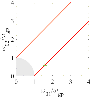
Figure 9: Possible combinations of $\omega_{01}$ and $\omega_{02}$ to have a real eigenfrequency in the parallel-parallel configuration are shown by the white area, and the gray area represents complex eigenfrequencies based on Eq. (19). Red curves satisfy Eq. (30) and show possible combinations of $\omega_{01}$ and $\omega_{02}$ that lead to a real EPD frequency. In these results, we kept $R_{g}$, $C_{1}$ and $C_{2}$ fixed as in Section III-B, and $L_{1}$ and $L_{2}$ are varied.

VI-A2 Parallel-Parallel Configuration

In order to get an EPD in the parallel-parallel configuration by using Eqs. (16), (17) and (18) the following condition must be satisfied:

$$\left(\omega_{01}-\omega_{02}\right)^{2}=\omega_{gp}^{2}.$$ (30)

For the parallel-parallel configuration we consider three different cases to choose the components’ values. First, if $\omega_{01}$ and $\omega_{02}$ are pure real, the value of $C_{1}$ or $C_{2}$ should be negative to have the same sign on both sides of Eq. (30). Hence, to have a real $\omega_{01}$ and $\omega_{02}$ one resonator should be made of both negative $C$ and $L$. Second, if both $\omega_{01}$ and $\omega_{02}$ have imaginary values, then $C_{1}$ and $C_{2}$ should have the same sign, either positive or negative. Finally, if just one of the $\omega_{01}$ or $\omega_{02}$ is imaginary and the other is real, there is no condition that leads to an EPD. In this paper, we considered the first scenario, where both $\omega_{01}$ and $\omega_{02}$ are real.

To have a real EPD frequency $\omega_{e}=\pm\sqrt{a}$, $a$ should be positive and this happens when Eq. (19) is satisfied. The region leading to $a>0$ is represented by the white area of Fig. 9, whereas the gray area represents the region with $a<0$. The red curves show different combinations of $\omega_{01}$ and $\omega_{02}$ which satisfy the EPD condition (30), assuming $\omega_{gp}$ constant. In this figure, $L_{1}=1/(\omega_{01}^{2}C_{1})$ and $L_{2}=1/(\omega_{02}^{2}C_{2})$ are varied, while $R_{g}$, $C_{1}$ and $C_{2}$ are constants. We have shown only results for the positive and real values of $\omega_{01}$ and $\omega_{02}$. The points on the red curves, which are located in the white area, can be selected to have an EPD with real and positive EPD frequency. The location marked by the green cross shows the values used for the example in Section III-B.

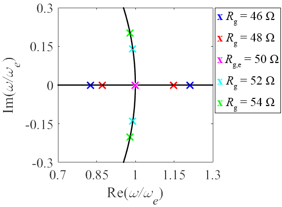
Figure 10: Root locus of zeros of $Z_{total}(\omega)$ shows the real and imaginary parts of resonance frequencies of the series-series configuration when varying gyration resistance. The EPD frequency corresponds to a double zero of the impedance.

VI-B Frequency Domain Analysis of The Degenerate Resonance

VI-B1 Series-Series Configuration

We show how the EPD regime is associated to a special kind of circuit’s resonance, directly observed in a frequency domain analysis of the circuit. We calculate the transferred impedance on the first side of the circuit in Fig. 2, that is

$$Z_{trans}(\omega)=\frac{R_{g}^{2}}{Z_{2}}.$$ (31)

where $Z_{2}(\omega)=j\omega L_{2}+1/(j\omega C_{2})$ is the series impedance on the right side of the circuit. Thus, the total impedance observed from the input port in this circuit is calculated by

$$Z_{total}(\omega)\triangleq Z_{1}(\omega)+Z_{trans}(\omega)=Z_{1}+\frac{R_{g}^{2}}{Z_{2}},$$ (32)

as shown in Fig. 2, where $Z_{1}(\omega)=j\omega L_{1}+1/(j\omega C_{1})$. The complex-valued resonant frequencies are obtained by imposing $Z_{total}(\omega)=0$. A few steps lead to the $\omega$-zeros given by Eq. (6). Fig. 10 shows the zeros of such total impedance $Z_{total}(\omega)$ for various gyration resistance values. When considering the EPD gyrator resistance $R_{g}=R_{g,e}=50\,\Omega$, one has $Z_{total}(\omega)\propto(\omega-\omega_{e})^{2}$, i.e., the two zeros coincide with the EPD angular frequency $\omega_{\mathrm{e}}$, that is also the point where the two curves in Fig. 10 meet. For gyrator resistances such that $R_{g}<R_{g,e}$, the two resonance angular frequencies are purely real. Instead, for $R_{g}>R_{g,e}$, the two resonance angular frequencies are complex conjugate, consistent with the result in Fig. 10. In other words, the EPD frequency coincides with double zeros, or double poles, of the frequency spectrum, depending on the way the circuit is described. In the past, EPD frequencies have been found by using loss and gain in a PT symmetry scheme [8, 9, 16], by including time-periodic modulation of a circuit element [34, 5, 17], and here by considering a gyrator and negative $L$ and $C$.

VI-B2 Parallel-Parallel Configuration

We calculate the total input admittance, $Y_{total}(\omega)$ (see Fig. 3), for the parallel-parallel circuit with the same approach discussed in the previous subsection. We define the two admittances of the resonators as $Y_{1}=j\omega C_{1}+1/(j\omega L_{1})$, $Y_{2}=j\omega C_{2}+1/(j\omega L_{2})$, and calculate the transferred admittance on the left side as

$$Y_{trans}(\omega)=\frac{1}{R_{g}^{2}Y_{2}}.$$ (33)

The total admittance $Y_{total}(\omega)$ is calculated as

$$Y_{total}(\omega)\triangleq Y_{1}(\omega)+Y_{trans}(\omega)=Y_{1}+\frac{1}{R_{g}^{2}Y_{2}}.$$ (34)

The resonant angular frequencies are obtained imposing $Y_{total}(\omega)=0$. A few steps lead to the same $\omega$-zeros given by Eq. (15). We calculate the resonance frequencies for various gyration resistance values in Fig. 11. When considering the EPD gyrator resistance $R_{g}=R_{g,e}=50\,\Omega$, one has $Y_{total}(\omega)\propto\left(\omega-\omega_{e}\right)^{2}$, i.e., the two zeros coincide, represented by the point where the two curves meet exactly at EPD angular frequency. For $R_{g}<R_{ge}$, resonance angular frequencies are complex conjugate pairs. Moreover, for $R_{g}>R_{g,e}$, the resonance angular frequencies are purely real, consistent with the result in Fig. 11.

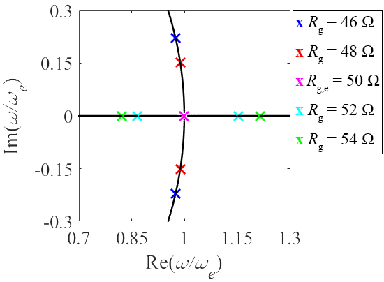
Figure 11: Root locus of zeros of $Y_{total}(\omega)$ shows the real and imaginary parts of resonance frequencies of the parallel-parallel configuration when varying gyration resistance. The EPD frequency corresponds to a double zero of the admittance.

VI-C Circuits Duality

The concept of duality applies to many fundamental physics/engineering concepts. For instance, this concept has been utilized many times in electromagnetic and electric circuits. Two circuits are dual if the mesh equations that describe one of them have the same mathematical form as the nodal equations that characterize another circuit [35]. Let us consider the mesh equations in the series-series configuration in Eq. (3) using Kirchhoff voltage law. According to the duality theorem, if we substitute voltage by current, current by voltage, capacitance by inductance, and inductance by capacitance, we obtain Eq. (12). So, we conclude that these two circuits are dual, and the properties of one can be obtained from the other.

VI-D The Coefficient of The Leading Term of The Puiseux Series

Using Eq. (27), we obtain the following expression for the coefficient of the leading term of the Puiseux series in the parallel-parallel configuration:

$$\alpha_{1}=\sqrt{\frac{\omega_{01}^{2}R_{g}^{2}\left(\omega_{e}^{2}-\omega_{02}^{2}\right)+\frac{\omega_{e}^{2}}{C_{1}C_{2}}}{\frac{1}{C_{1}C_{2}}+R_{g}^{2}\left(\omega_{01}^{2}+\omega_{02}^{2}-6\omega_{e}^{2}\right)}},$$ (35)

when we perturb the capacitance. Instead, when we perturb the inductance, the coefficient is

$$\alpha_{1}=\sqrt{\frac{\omega_{01}^{2}R_{g}^{2}\left(\omega_{e}^{2}-\omega_{02}^{2}\right)}{\frac{1}{C_{1}C_{2}}+R_{g}^{2}\left(\omega_{01}^{2}+\omega_{02}^{2}-6\omega_{e}^{2}\right)}}.$$ (36)

VI-E The impedance inverter

There are several circuits that can provide for negative capacitances and inductances needed for the gyrator-based EPD circuits. Opamp-based circuits can be used as impedance inverter. Two circuits to obtain negative impedance are shown in Fig. 12. The circuit in Fig. 12(a) converts the impedance $Z_{l}(\omega)$ to $Z_{in}(\omega)=-Z_{l}(\omega)$. When $Z_{l}(\omega)$ in the circuit in Fig. 12(a) is a single capacitor, i.e., $Z_{l}(\omega)=1/(j\omega C)$, we obtain $Z_{in}(\omega)=-1/(j\omega C)$ at the input port. On the other hand, for realizing a negative inductance using a single capacitor in $Z_{l}(\omega)=1/(j\omega C)$, the circuit displayed in Fig. 12(b) is utilized leading to $Z_{in}(\omega)=(-R^{2}C)j\omega$. Desired negative inductance values are achieved with proper sets of values for $R$ and $C$. Hence, we can employ these circuits to generate a negative capacitance and a negative inductance by only using loads with a single capacitance.

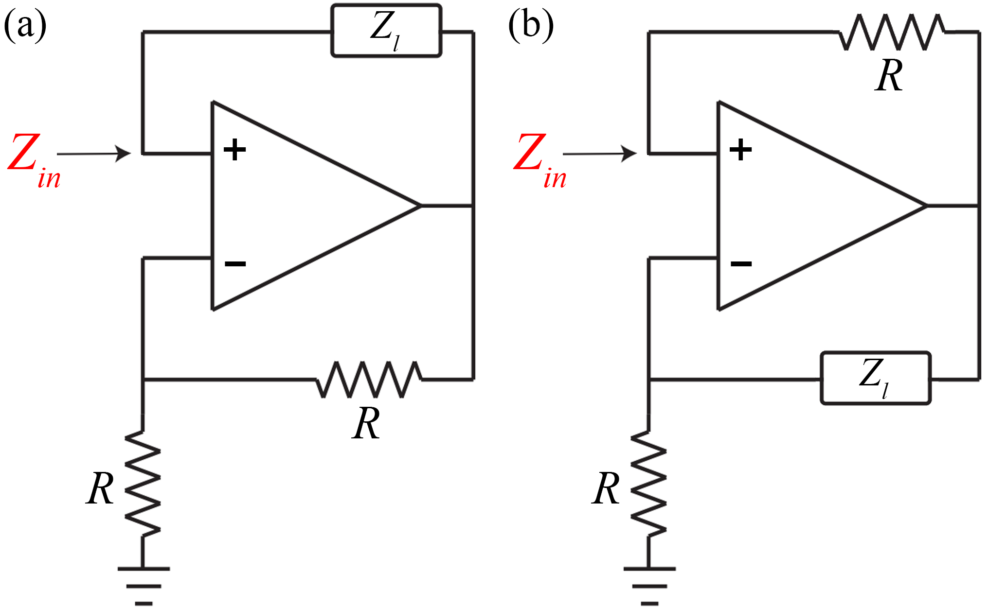
Figure 12: Negative impedance converter circuit implementation by using an opamp to achieve (a) a negative capacitance, and (b) a negative inductance, assuming $Z_{l}(\omega)=1/(j\omega C)$ is capacitive.

References

- [1] A. Figotin and I. Vitebskiy, “Oblique frozen modes in periodic layered media,” Physical Review E, vol. 68, no. 3, p. 036609, Sep 2003.
- [2] M. A. K. Othman, F. Yazdi, A. Figotin, and F. Capolino, “Giant gain enhancement in photonic crystals with a degenerate band edge,” Physical Review B, vol. 93, no. 2, p. 024301, Jan 2016.
- [3] M. A. K. Othman, X. Pan, G. Atmatzakis, C. G. Christodoulou, and F. Capolino, “Experimental demonstration of degenerate band edge in metallic periodically loaded circular waveguide,” IEEE Transactions on Microwave Theory and Techniques, vol. 65, no. 11, pp. 4037–4045, Nov 2017.
- [4] A. F. Abdelshafy, M. A. K. Othman, D. Oshmarin, A. T. Almutawa, and F. Capolino, “Exceptional points of degeneracy in periodic coupled waveguides and the interplay of gain and radiation loss: Theoretical and experimental demonstration,” IEEE Transactions on Antennas and Propagation, vol. 67, no. 11, pp. 6909–6923, Nov 2019.
- [5] H. Kazemi, M. Y. Nada, T. Mealy, A. F. Abdelshafy, and F. Capolino, “Exceptional points of degeneracy induced by linear time-periodic variation,” Physical Review Applied, vol. 11, no. 1, p. 014007, Jan 2019.
- [6] K. Rouhi, H. Kazemi, A. Figotin, and F. Capolino, “Exceptional points of degeneracy directly induced by space-time modulation of a single transmission line,” IEEE Antennas and Wireless Propagation Letters, vol. 19, no. 11, pp. 1906 – 1910, Nov 2020.
- [7] C. M. Bender and S. Boettcher, “Real spectra in non-Hermitian Hamiltonians having PT symmetry,” Physical Review Letters, vol. 80, no. 24, pp. 2455–2464, Jun 1998.
- [8] W. D. Heiss, “Exceptional points of non-Hermitian operators,” Journal of Physics A: Mathematical and General, vol. 37, no. 6, pp. 2455–2464, Jan 2004.
- [9] J. Schindler, A. Li, M. C. Zheng, F. M. Ellis, and T. Kottos, “Experimental study of active LRC circuits with PT symmetries,” Physical Review A, vol. 84, no. 4, p. 040101, Oct 2011.
- [10] M. V. Berry, “Physics of nonhermitian degeneracies,” Czechoslovak journal of physics, vol. 54, no. 10, pp. 1039–1047, Oct 2004.
- [11] J. Wiersig, “Enhancing the sensitivity of frequency and energy splitting detection by using exceptional points: application to microcavity sensors for single-particle detection,” Physical Review Letters, vol. 112, no. 20, p. 203901, 2014.
- [12] W. Chen, S. Kaya Ozdemir, G. Zhao, J. Wiersig, and L. Yang, “Exceptional points enhance sensing in an optical microcavity,” Nature, vol. 548, no. 7666, pp. 192–196, Aug 2017.
- [13] W. Chow, J. Gea-Banacloche, L. Pedrotti, V. Sanders, W. Schleich, and M. Scully, “The ring laser gyro,” Reviews of Modern Physics, vol. 57, no. 1, p. 61, 1985.
- [14] S. Sunada and T. Harayama, “Design of resonant microcavities: application to optical gyroscopes,” Optics express, vol. 15, no. 24, pp. 16 245–16 254, 2007.
- [15] Q. Wang and Y. Liu, “Review of optical fiber bending/curvature sensor,” Measurement, vol. 130, pp. 161–176, 2018.
- [16] P.-Y. Chen, M. Sakhdari, M. Hajizadegan, Q. Cui, M. M.-C. Cheng, R. El-Ganainy, and A. Alu, “Generalized parity-time symmetry condition for enhanced sensor telemetry,” Nature Electronics, vol. 1, no. 5, pp. 297–304, May 2018.
- [17] H. Kazemi, A. Hajiaghajani, M. Y. Nada, M. Dautta, M. Alshetaiwi, P. Tseng, and F. Capolino, “Ultra-sensitive radio frequency biosensor at an exceptional point of degeneracy induced by time modulation,” IEEE Sensors Journal, vol. 21, no. 6, pp. 7250–7259, Mar 2021.
- [18] B. D. Tellegen, “The gyrator, a new electric network element,” Philips Res. Rep, vol. 3, no. 2, pp. 81–101, 1948.
- [19] R. Inigo, “Gyrator realization using two operational amplifiers,” IEEE Journal of Solid-State Circuits, vol. 6, no. 2, pp. 88–89, Apr 1971.
- [20] C. L. Hogan, “The ferromagnetic faraday effect at microwave frequencies and its applications,” Bell System Technical Journal, vol. 31, no. 1, pp. 1–31, Jan 1952.
- [21] A. Figotin, “Synthesis of lossless electric circuits based on prescribed Jordan forms,” Journal of Mathematical Physics, vol. 61, no. 12, p. 122703, 2020.
- [22] A. Figotin, “Perturbations of circuit evolution matrices with Jordan blocks,” Journal of Mathematical Physics, vol. 62, no. 4, p. 042703, Apr 2021.
- [23] C. R. White, J. W. May, and J. S. Colburn, “A variable negative-inductance integrated circuit at UHF frequencies,” IEEE Microwave and Wireless Components Letters, vol. 22, no. 1, pp. 35–37, Jan 2012.
- [24] E. H. Kopp, “Negative impedance inverter circuits,” in Proceedings of the IEEE, vol. 53, no. 12, pp. 2125–2126, Dec 1965.
- [25] P. Horowitz and W. Hill, The art of electronics. Cambridge Univ. Press, 1989.
- [26] M. Ershov, H. Liu, L. Li, M. Buchanan, Z. Wasilewski, and A. Jonscher, “Negative capacitance effect in semiconductor devices,” IEEE Transactions on Electron Devices, vol. 45, no. 10, pp. 2196–2206, 1998.
- [27] S.-G. Yang, G.-H. Ryu, and K.-S. Seo, “Fully symmetrical, differential-pair type floating active inductors,” IEEE International Symposium on Circuits and Systems (ISCAS), 1997.
- [28] S. E. Khoury, “New approach to the design of active floating inductors in MMIC technology,” IEEE Transactions on Microwave Theory and Techniques, vol. 44, no. 4, pp. 505–512, Apr 1996.
- [29] T. Kato, Perturbation Theory for Linear Operators, 2nd ed. Springer-Verlag, Berlin Heidelberg, 1995, vol. 132.
- [30] B. Shenoi, “Practical realization of a gyrator circuit and rc-gyrator filters,” IEEE Transactions on Circuit Theory, vol. 12, no. 3, pp. 374–380, 1965.
- [31] A. Antoniou and K. Naidu, “Modeling of a gyrator circuit,” IEEE Transactions on Circuit Theory, vol. 20, no. 5, pp. 533–540, 1973.
- [32] A. Welters, “On explicit recursive formulas in the spectral perturbation analysis of a Jordan block,” SIAM Journal on Matrix Analysis and Applications, vol. 32, no. 1, pp. 1–22, Jan 2011.
- [33] H. Hodaei, A. U. Hassan, S. Wittek, H. Garcia-Gracia, R. El-Ganainy, D. N. Christodoulides, and M. Khajavikhan, “Enhanced sensitivity at higher-order exceptional points,” Nature, vol. 548, no. 7666, pp. 187–191, Aug 2017.
- [34] H. Kazemi, M. Y. Nada, A. Nikzamir, F. Maddaleno, and F. Capolino, “Experimental demonstration of exceptional points of degeneracy in linear time periodic systems and exceptional sensitivity,” arXiv preprint arXiv:1908.08516, 2019.
- [35] N. Balabanian, S. Seshu, and T. A. Bickart, Electrical network theory. Wiley, 1969.