Hunting dark energy with pressure-dependent photon-photon scattering
— Dedicated to the late professor Yasunori Fujii —

Abstract

Toward understanding of dark energy, we propose a novel method to directly produce a chameleon particle and force its decay under controlled gas pressure in a laboratory-based experiment. Chameleon gravity, characterized by its varying mass depending on its environment, could be a source of dark energy, which is predicted in modified gravity. A remarkable finding is a correspondence between the varying mass and a characteristic pressure dependence of a stimulated photon-photon scattering rate in a dilute gas surrounding a focused photon-beam spot. By observing a steep pressure dependence in the scattering rate, we can directly extract the characteristic feature of the chameleon mechanism. As a benchmark model of modified gravity consistent with the present cosmological observations, a reduced $F(R)$ gravity is introduced in the laboratory scale. We then demonstrate that the proposed method indeed enables a wide-ranging parameter scan of such a chameleon model with the varying mass around $(0.1-1)~{}[\mu\mathrm{eV}]$ by controlling pressure values.

I Introduction

A variety of independent observations have confirmed the accelerated expansion of the Universe, which indicates an unknown energy called dark energy (DE). Modified gravity theory has been considered one of the solutions to the DE problem as an alternative to the ad hoc introduction of the cosmological constant to general relativity. Among the modified gravity theories, scalar-tensor theory introduces a new scalar field Caldwell et al. (1998); Peebles and Ratra (2003); Copeland et al. (2006). This scalar field plays a role of dynamical DE, and its coupling to ordinary matter induces the so-called fifth force. The phenomenology of the new scalar field and the induced fifth force have been developed to constrain modified gravity: possible deviations from the gravitational inverse-square law Will (2014); Adelberger et al. (2003); Spero et al. (1980); Kapner et al. (2007) and time-varying parameters of the standard model of particle physics Marion et al. (2003); Peik et al. (2004); Damour and Dyson (1996); Srianand et al. (2004).

It is known that a dilatonic scalar field shows up in modified gravity for DE through the Weyl transformation of the metric De Felice and Tsujikawa (2010); Nojiri and Odintsov (2011); Clifton et al. (2012); Capozziello and De Laurentis (2011); Nojiri et al. (2017). A class of such a dilaton is called chameleon field, which is named after a remarkable feature of the environment dependence, the chameleon mechanism Khoury and Weltman (2004). The coupling to matter influences the effective mass of the chameleon field, which is analogous to an in-medium mass (an effective mass) in heavy fermion materials. Consequently, the chameleon mechanism screens the fifth force in a high-density environment, which allows the modified gravity to be consistent with short-scale local experiments and observations.

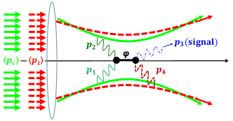
Figure 1: Concept of stimulated resonant photon-photon scattering in quasiparallel collision geometry.

There have been attempts to search for the chameleon field using nongravitational experiments Burrage and Sakstein (2018); Chou et al. (2009); Steffen et al. (2010); Rybka et al. (2010); Brax et al. (2009); Anastassopoulos et al. (2019); Levshakov et al. (2010); Vagnozzi et al. (2021). Recently, it was suggested that a stimulated radar-collider concept may be applicable to probe gravitationally coupled scalar fields Homma and Kirita (2020), as illustrated in Fig. 1. The method resonantly produces a low-mass scalar field $\varphi$ in quasiparallel photon-photon scattering and simultaneously stimulates its decay by combining two different frequency photon beams along the same optical axis and focusing them into a vacuum. As a consequence of the stimulated resonant scattering, a frequency-shifted photon can be generated as a clear signal of scattering. This provides the possibility of directly exploring the microscopic nature relevant to DE through the photon-photon scattering experiment, despite the fact that the coupling strength considered to be of the order of (or even less than) the gravitational constant.

We find a new and remarkable potential to probe the chameleon particle and the chameleon mechanism in the stimulated photon-photon scattering experiment in Homma and Kirita (2020). It is possible to directly extract the chameleon mechanism via a correspondence between the varying mass and a characteristic pressure dependence of the stimulated photon-photon scattering rate in a dilute gas surrounding a focused photon-beam spot. The methodology is applied to test a class of chameleon models predicted in the viable DE models of $F(R)$ gravity Nunes et al. (2017). We discuss the pressure dependence of the signal in viable parameter spaces of the Starobinsky model Starobinsky (2007) and the Hu-Sawicki model Hu and Sawicki (2007), which are widely used in late-time cosmology. It will be shown that the pressure dependence can be observed as a signal photon number with a tenth power steepness, which is clearly separable from the background atomic process.

II Extendable chameleon mass: coupling domain

We begin with the theoretical basis on the chameleon field and show the expected sensitivity to probe the chameleon field using the experimental idea given in Homma and Kirita (2020) projected onto the mass-coupling space. A chameleon field $\phi$ coupling to matter fields is described in scalar-tensor theory as

$$S= \int d^{4}x\sqrt{-g_{*}}\left[\frac{M^{2}_{\mathrm{pl}}}{2}R_{*}-\frac{1}{2}g_{*}^{\mu\nu}(\partial_{\mu}\varphi)(\partial_{\nu}\varphi)-V(\varphi)\right]$$

$$\qquad+\int d^{4}x\sqrt{-g_{*}}\mathcal{L}_{\mathrm{M}}\left[g^{\mu\nu}_{*},\varphi,\Phi_{i}\right]\,,$$ (1)

where $\mathcal{L}_{\mathrm{M}}$ is the Lagrangian density of arbitrary matter fields $\Phi_{i}$ and $M_{\mathrm{pl}}$ is the reduced Planck mass, $M_{\mathrm{pl}}\simeq 2.44\times 10^{27}~{}[\mathrm{eV}]$. The Einstein frame metric $g_{*\mu\nu}$ and the Jordan frame metric $g_{\mu\nu}$ are related to each other via $g_{*\mu\nu}=\mathrm{e}^{2\beta_{i}\varphi/M_{\mathrm{pl}}}g_{\mu\nu}$. In general, scalar-tensor theory allows us to parametrize the coupling constants $\beta_{i}$ between the chameleon $\varphi$ and other fields $\Phi_{i}$. We conventionally define the effective potential of the chameleon field as follows:

$$V_{\mathrm{eff}}(\varphi)\equiv V(\varphi)-\frac{1}{4}\sum_{i}e^{-\frac{4\beta_{i}\varphi}{M_{\mathrm{pl}}}}T^{\mu}_{\ \mu(i)}\,,$$ (2)

where $T_{\mu\nu(i)}$ is the energy-momentum tensor of $\Phi_{i}$ in the Jordan frame.  Because of the dilatonic coupling between $\varphi$ and $T^{\mu}_{\ \mu}$, the effective potential and the chameleon mass acquire the environment dependence which drives the chameleon mechanism.

The chameleon can interact with the electromagnetic field through the quantum trace anomaly, which generates the coupling to two photons. This coupling generation can be viewed through the anomalous Weyl transformation Fujikawa (1980); Fujii (2016); Ferreira et al. (2017); Katsuragawa and Matsuzaki (2017), and the derived interaction terms can be cast in the following form:

$$\begin{split}\mathcal{L}_{\mathrm{M}}&=\frac{1}{4}e^{-\frac{4\beta_{\gamma}\varphi}{M_{\mathrm{pl}}}}T^{\mu}_{\ \mu(\mathrm{anomaly})}\\ &=-\frac{1}{4}e^{-\frac{4\beta_{\gamma}\varphi}{M_{\mathrm{pl}}}}\left(\frac{b_{\mathrm{em}}\cdot\alpha_{\rm em}}{8\pi}F_{\mu\nu}F^{\mu\nu}\right)\,.\end{split}$$ (3)

Here $\alpha_{\rm em}$ is the fine-structure constant of the electromagnetic coupling and $b_{\rm em}$ denotes a beta function coefficient which would include all the charged particle contributions at the loop level of the standard model of particle physics: $b_{\rm em}=11/3$ at the one-loop level. The relevant interaction between the chameleon and the photons is thus written as 

$$\mathcal{L}_{\mathrm{\varphi\gamma\gamma}} =\frac{1}{4}\frac{\tilde{\beta}_{\gamma}\varphi}{M_{\mathrm{pl}}}F_{\mu\nu}F^{\mu\nu}\,,\ \tilde{\beta}_{\gamma}\equiv\frac{b_{\rm em}\cdot\alpha_{\mathrm{em}}}{2\pi}\beta_{\gamma}\,.$$ (4)

Furthermore, various matter consisting of an experimental environment may also contribute to the chameleon mechanism. The matter contribution is cast into the matter energy density $T^{\mu}_{\mu}\approx-\rho_{\mathrm{m}}$, which is evaluated in each chameleon-search experiment.

Based on the following parametrization, 

$$V_{\mathrm{eff}}(\varphi)=V(\varphi)+\frac{1}{4}F_{\mu\nu}F^{\mu\nu}e^{\frac{\tilde{\beta}_{\gamma}\varphi}{M_{\mathrm{pl}}}}+\rho_{\mathrm{m}}e^{\frac{\beta_{\mathrm{m}}\varphi}{M_{\mathrm{pl}}}}\,,$$ (5)

the nongravitational experiments placed the limit on $\tilde{\beta}_{\gamma}$ Burrage and Sakstein (2018). In Fig. 2 we summarize current constraints and the expected detection sensitivity in the stimulated radar collider Homma and Kirita (2020) in the mass-coupling parameter space.  GammeV CHameleon Afterglow SEarch (GammeV-CHASE) constrains $\tilde{\beta}_{\gamma}\lesssim 7.1\times 10^{10}$ when $m_{\varphi}\lesssim\mathcal{O}(10^{-3})~{}[\mathrm{eV}]$ Steffen et al. (2010). In terms of the beyond-the-standard-model (BSM) particle-search experiments, the Axion Dark Matter Experiment (ADMX) excluded $2\times 10^{9}\lesssim\tilde{\beta}_{\gamma}\lesssim 5\times 10^{14}$ for $m_{\varphi}\sim 1.95~{}[\mathrm{\mu eV}]$ Rybka et al. (2010), and the collider experiments placed the limit $\tilde{\beta}_{\gamma}\lesssim 2\times 10^{15}$ for $10^{-11}~{}[\mathrm{eV}]\lesssim m_{\varphi}\lesssim 10^{4}~{}[\mathrm{eV}]$ Brax et al. (2009). We note that the CERN Axion Solar Telescope has placed the limit on the coupling space ($\beta_{m}$, $\tilde{\beta}_{\gamma}$) as $\tilde{\beta}_{\gamma}\lesssim 5.7\times 10^{10}$ for $1<\beta_{m}<10^{6}$ Anastassopoulos et al. (2019).

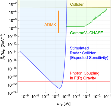
Figure 2: Expected detection sensitivity of the chameleon field in the presently proposed photon-photon scattering experiment (blue region) by focusing two pulses with $100~{}[\mathrm{J/ns}]$ consisting of gigahertz-band photons in the quasiparallel geometry evaluated in Ref. Homma and Kirita (2020). The red horizontal line corresponds to the chameleon-photon coupling $\tilde{\beta}_{\gamma}=\frac{b_{\rm em}\alpha_{\rm em}}{2\sqrt{6}\pi}$ when we take $\beta_{\gamma}=\frac{1}{\sqrt{6}}$ in Eq. (4). The chameleon in $F(R)$ gravity is hunted along the red line that overlaps with the detection sensitivity domain. Constraints from GammeV-CHASE (green region), ADMX (orange line), and collider experiments (yellow region) are shown for comparison.

As evident in Fig. 2, the simulated radar-collider experiment in Homma and Kirita (2020) can improve the current constraints on $\tilde{\beta}_{\gamma}$ in terms of scalar-tensor theory by more than the tenth order of magnitude. 

III Chameleon in $F(R)$ gravity

When one takes full advantage of the accessibility to $\tilde{\beta}_{\gamma}\lesssim\mathcal{O}(1)$, $F(R)$ gravity can provide a suitable benchmark model of the chameleon. $F(R)$ stands for a function of the Ricci scalar $R$, and the Einstein-Hilbert action of the general relativity is replaced by $F(R)$. By the Weyl transformation defined as $\mathrm{e}^{2\sqrt{1/6}\varphi/M_{\mathrm{pl}}}\equiv F_{R}(R)$, $F(R)$ gravity turns into a specific case of scalar-tensor theory [Eq. (1)]. Here the subscript $R$ for $F(R)$ denotes the derivative with respect to $R$. The potential $V(\varphi)$ is written as a function of the Ricci scalar,

$$V(\varphi)\equiv\frac{M^{2}_{\mathrm{pl}}}{2}\frac{R(\varphi)F_{R}(R(\varphi))-F(R(\varphi))}{F_{R}^{2}(R(\varphi))}\,.$$ (6)

Unlike in generic scalar-tensor theory, the coupling constant $\beta_{i}$ in Eq. (2) is not parametric, but rather fixed as $\beta_{i}=1/\sqrt{6}$ for all matter fields in $F(R)$ gravity Maeda (1989). In terms of Eq. (5), $F(R)$ gravity gives $\tilde{\beta}_{\gamma}=\mathcal{O}(10^{-3})$ and $\beta_{\mathrm{m}}=\mathcal{O}(1)$, which eludes those in the existing nongravitational tests. Because the coupling constants are independent of $F(R)$ function, $F(R)$ gravity models are testable if they predict chameleon fields with masses around $m_{\varphi}=(0.1-1)~{}[\mathrm{\mu eV}]$ as in Fig 2.

IV Matter sources for chameleon effects

In Eq. (2), we have mainly two ambient sources, photon and gas densities, in scanning the effective mass of the chameleon,

$$T^{\mu}_{\ \mu}=T^{\mu}_{\ \mu(\mathrm{photon})}+T^{\mu}_{\ \mu(\mathrm{gas})}\,.$$ (7)

We evaluate those two ingredients in $T^{\mu}_{\ \mu}$ in light of the proposed experimental setup. The photon contribution in Eq. (4) goes like $T^{\mu}_{\ \mu(\mathrm{photon})}\propto F_{\mu\nu}F^{\mu\nu}=2(\mathbf{B}^{2}-\mathbf{E}^{2})$, with the electric field $\mathbf{E}$ and magnetic field $\mathbf{B}$. This contribution vanishes in the case with the ordinary plane electromagnetic wave where $\mathbf{E}$ and $\mathbf{B}$ have the same amplitude, while in the case of the focused geometry in Fig.1 amplitudes of the electric and magnetic fields are given by nontrivial spatial distribution functions (as is explained in the Appendix A ). It turns out, however, that the square of the field strength vanishes at each point on the focal plane in the case of circularly polarized beams Wolf (1959); Richards and Wolf (1959); Stamnes (2017). Therefore, with the circularly polarized beams proposed in Homma and Kirita (2020), we can ignore the contribution from the background photon density. 

Regarding the gas contribution, we assume the conventional perfect-fluid description because of the difficulties in treating the atoms or molecules using the fundamental field prescription. Then the trace of the energy-momentum tensor is evaluated as $T^{\mu}_{\ \mu(\mathrm{gas})}=-(\rho-3P)$, where $\rho$ and $P$ represent the density and pressure, respectively. Gas in an experimental chamber exhibits a low pressure ($P\ll\rho$) and a high temperature; hence, we assume the equation of state for the ideal gas. In that case the trace of the energy-momentum tensor can be approximated as follows:

$$-T^{\mu}_{\ \mu(\mathrm{gas})}\approx\rho~{}[\mathrm{kg/m^{3}}]=\frac{P~{}[\mathrm{Pa}]}{\mathcal{R}T}\,,$$ (8)

where $T~{}[\mathrm{K}]$ is the temperature and $\mathcal{R}$ is the specific gas constant. $\mathcal{R}$ is defined as the molar gas constant $\mathcal{R}_{u}$ divided by the molar mass of the gas $M~{}[\mathrm{kg/mol}]$, $\mathcal{R}=\mathcal{R}_{u}/M$, where $\mathcal{R}_{u}=8.31446~{}[\mathrm{m^{3}\cdot Pa\cdot K^{-1}\cdot mol^{-1}}]$.

In the proposed setup we assume an ultrahigh vacuum chamber to reduce background frequency-shifted photons caused by the residual atoms, and such a low-density environment also weakens the chameleon mechanism. However, because the gas density is controllable by the gas pressure, as in Eq. (8), over several orders of magnitude, in principle, we can measure how the signal is weakened as a function of the gas pressure, which is the characteristic feature of the chameleon mechanism.

V Reduced $F(R)$ form for modeling DE

As one of cosmological models in $F(R)$ gravity, let us consider the $R^{2}$-corrected DE models Appleby et al. (2010):

$$F(R)=R+f_{\mathrm{DE}}(R)+\alpha R^{2}$$ (9)

where $\alpha$ is a positive parameter. The second term $f_{\mathrm{DE}}(R)$ represents the modification for DE, and the third term $\alpha R^{2}$ cures the singularity problem in generic $f_{\mathrm{DE}}(R)$ models Frolov (2008); Nojiri and Odintsov (2008). As representatives of $f_{\mathrm{DE}}(R)$, we consider the Starobinsky model Starobinsky (2007) and the Hu-Sawicki model Hu and Sawicki (2007), which have been widely used in the study of late-time cosmology.

By considering a fact that the typical energy scale is higher than the DE scale in the laboratory environment, it is unnecessary to adopt the exact form of $f_{\mathrm{DE}}(R)$. The large-curvature limit $R/R_{c}\gg 1$, where $R_{c}$ corresponds to the current vacuum curvature, is a good enough approximation for local experiments. In the large-curvature limit, the above two models are reduced to the same form (as explained in Appendix B), and Eq. (9) approximates to the following:

$$F(R)=R-\lambda R_{c}\left[1-\left(\frac{R}{R_{c}}\right)^{-2n}\right]+\alpha R^{2}\,,$$ (10)

where $\lambda$ and $n$ are positive parameters. The coefficient $\lambda R_{c}$ in the second term can be considered the cosmological constant $\lambda R_{c}=2\Lambda$, where $\Lambda\simeq 4.2\times 10^{-66}\ [\mathrm{eV}^{2}]$ Aghanim et al. (2020). In this paper, we adopt Eq. (10) to investigate the $R^{2}$-corrected Starobinsky and Hu-Sawicki models in a laboratory-based experiment, thereby respecting a parameter space $(\lambda,n)$ that is consistent with the cosmological observations.

VI Chameleon mass dependence on the reduced $F(R)$ parameters

Next, we study the chameleon mass under the background gas pressure surrounding the scattering point, equivalently, the gas density with a fixed volume in the experimental chamber. The second derivative of the effective potential at the potential minimum gives the chameleon mass $m_{\varphi}$. Using Eq. (6), we can write the chameleon mass formula in terms of the $F(R)$ function and its derivatives:

$$\begin{split}m_{\varphi}^{2}&=V(\varphi_{\min})_{\mathrm{eff},\varphi\varphi}\\ &=\frac{1}{3F_{RR}(R_{\min})}\left[1-\frac{R_{\min}F_{RR}(R_{\min})}{F_{R}(R_{\min})}\right]\end{split}$$ (11)

where $R_{\min}$ is determined by the stationary condition $V(\varphi_{\min})_{\mathrm{eff},\varphi}=0$ given by $2F(R_{\min})-R_{\min}F_{R}(R_{\min})+\kappa^{2}T^{\mu}_{\mu}=0$. In the limit where $R/R_{c}\gg 1$, the stationary condition gives $R_{\min}\approx-\kappa^{2}T^{\mu}_{\mu}$ in the model [Eq. (10)]. Using the relation $2\Lambda=\lambda R_{c}$, we obtain the chameleon mass in the analytic form as Katsuragawa and Matsuzaki (2018)

$$m_{\varphi}^{2} =\frac{\Lambda}{12n(2n+1)\left(\frac{\lambda}{2}\right)^{-2n}\left(-\frac{T^{\mu}_{\mu}}{\rho_{\Lambda}}\right)^{-2(n+1)}+6\alpha\Lambda}\,,$$ (12)

where we have defined the DE density as $\rho_{\Lambda}\equiv\Lambda/\kappa^{2}$ and taken the limit $\Lambda\ll R\ll 1/\alpha$.

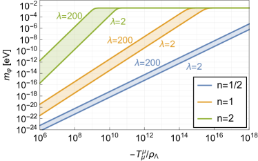
Figure 3: Chameleon mass vs energy-momentum tensor in Eq. (12) for $n=1/2,1,2$ with $\Lambda=4.2\times 10^{-66}\ [\mathrm{eV}^{2}]$. For each $n$, $\lambda=2$ and $\lambda=200$ correspond to left and right solid lines, respectively. As a referenced value, we have chosen $\alpha=10^{4}~{}[\mathrm{eV^{-2}}]$ to be consistent with the current constraint from the fifth-force experiment, $\alpha\leq 2.3\times 10^{4}~{}[\mathrm{eV^{-2}}]$ Cembranos (2009).

Figure 3 shows the chameleon mass given in Eq. (12) as a function of $T^{\mu}_{\ \mu}$ when one varies $\lambda$ from $2$ to $200$. This range of $\lambda$ overlaps with the cosmological constraint at the $2\sigma$ confidence level Nunes et al. (2017) for the Starobinsky model with $n=1$ and for the Hu-Sawicki model with $n=1/2$. For a general $n$, a larger $\lambda$ may be allowed because $\lambda\rightarrow\infty$ at $\lambda R_{c}=2\Lambda$ corresponds to the $\Lambda$ cold dark matter model.

We apply the model to a low pressure interval $10^{-8}~{}[\mathrm{Pa}]<P<10^{-6}~{}[\mathrm{Pa}]$ within the reach of the current vacuum technology. In such an ultrahigh vacuum chamber, the residual gas consists mainly of hydrogen molecules, and Eq. (8) for the hydrogen at $T=300~{}[\mathrm{K}]$ gives

$$1.4\times 10^{12} \lesssim-\frac{T^{\mu}_{\mu}}{\rho_{\Lambda}}\lesssim 1.4\times 10^{14}\,$$ (13)

with the observed DE density $\rho_{\Lambda}\sim 2.5\times 10^{-11}~{}[\mathrm{eV^{4}}]$. In using other gas species, one can multiply the ratio of molecular weight to that of hydrogen molecule with the above $(-\frac{T^{\mu}_{\mu}}{\rho_{\Lambda}})$ value. As a benchmark, in Eq. (12) we may choose $\alpha=10^{4}~{}[\mathrm{eV^{-2}}]$ as in Fig. 3. For the range $\lambda=2$–$200$, the case $n=1$ predicts the chameleon in the testable range as in Fig. 2. The case $n=1/2$ is also testable by raising the gas pressure or changing the gas species, although larger $\lambda$ for $n=1/2$ is testable even in the current setup. Note that the case $n=2$ predicts heavy masses outside the sensitivity $m_{\varphi}\simeq 4.1\times 10^{-3}~{}[\mathrm{eV}]$.

VII Feasibility to extract the chameleon character

The key feature of the chameleon exchange appears in its density dependence of the stimulated resonant scattering rate. Figure 4 shows the expected number of signal photons as a function of gas pressure comprising hydrogen molecules at $300~{}[\mathrm{K}]$ for an $n=1$ with $\lambda=$ 2, 20, and 200 cases. The signal yield is proportional to $\tilde{\beta_{\gamma}}^{2}$ with the set of parameters used in Homma and Kirita (2020), which assumed two beams with the same pulse energy of $100~{}[\mathrm{J}]$.  The pressure range where the signal yield exceeds unity is the region of interest to test chameleon models.

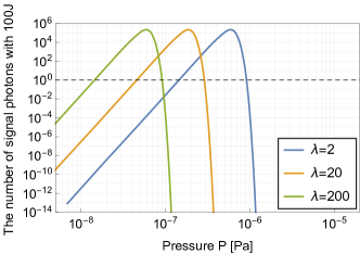
Figure 4: Expected number of stimulated signal photons as a function of gas pressure comprising hydrogen molecules at $300~{}[\mathrm{K}]$ for an $n=1$ with $\lambda=$ 2, 20, and 200 cases. The signal yield is calculated by assuming the photon-chameleon coupling defined in Eq. (4) and the set of experimental parameters used in Homma and Kirita (2020), with the same pulse energy of $100~{}[\mathrm{J}]$ for the two beams. The dashed horizontal line shows unity above which experiments can test the characteristic features of chameleon models. To evaluate the dependence for other types of molecules with molar mass $M$, one can scale the pressure values by multiplying $M_{{H}_{2}}/M$ with the molar mass of hydrogen molecule $M_{{H}_{2}}$.

As for background processes, four-wave mixing (FWM) via residual atoms produces photon energies that are kinematically similar to those of the signal via energy-momentum conservation J. and E. (1981). The photon yield from the atomic FWM process is known to be proportional to the square of the third order polarization susceptibility $\chi^{(3)}$. Because $\chi^{(3)}$ is proportional to the number density of the atoms, and hence to gas pressure, the atomic FWM yield is expected to have a quadratic pressure dependence, and this dependence has indeed been observed in the actual searching setup in laser frequencies Hasebe et al. (2015); Nobuhiro et al. (2020); Homma et al. (2021), although the yield is expected to be negligibly small. 

We further note that only the possible standard model process in vacuum, light-by-light scattering induced by a box diagram in quantum electrodynamics, is also negligible in the mass range $(0.1-1)~{}[\mu\mathrm{eV}]$ due to the sixth-power dependence of the cross section on the center-of-mass system energy even if we take the effect of stimulation into account Homma and Toyota (2017). The power exponent on the lower pressure side is around 10 for $n=1$, which is clearly distinguishable from the quadratic pressure dependence of the background atomic FWM process and also separable from pressure-independent BSM signals, if there are any. Therefore, in principle, the proposed method can provide firm grounds to purely test the chameleon mechanism separably from backgrounds in laboratory experiments.

VIII Conclusion

In conclusion, hunting chameleons as DE is possible by measuring the pressure-dependent stimulated photon-photon scattering in a laboratory-based radar-collider experiment. If two focused radar pulses with $100~{}[\mathrm{J/ns}]$ are each available as designed in Homma and Kirita (2020), the chameleon model with a cosmologically allowed parameter space, $n=1$ with a wide range of $\lambda=2$–$200$, is testable based on the tenth-power steep pressure dependence of the signal yield with a chameleon mass in the range $(0.1-1)~{}[\mu\mathrm{eV}]$. This observable can clearly discriminate chameleons from other background processes. Therefore, the proposed method can provide a unique opportunity to strictly constrain the viable $F(R)$ gravity models for DE, which can be consistent with the current cosmological observations. Given future developments on the microwave technologies and a capability for accurate pressure control, this method will pave the way to directly unveil dark energy in the completely controlled manner.

Appendix A Electromagnetic Field in a Focused Photon Beam

A.1 Setup for Focusing Optics

We consider the electric field $\mathbf{E}$ and magnetic field $\mathbf{B}$ in the focusing optics. The wave equation in vacuum goes like

$$\Box\mathbf{F}(\mathbf{r},t)=0\,.$$ (14)

Its solution $\mathbf{F}(\mathbf{r},t)$ is expressed in terms of the complex amplitude as

$$\mathbf{F}(\mathbf{r},t)=\frac{1}{2}\hat{\mathbf{F}}(\mathbf{r})e^{-i\omega t}+{\rm c.c}.\,.$$ (15)

Then the amplitude $\hat{\mathbf{F}}(\mathbf{r})$ satisfies the Helmholtz equation,

$$\left(\nabla^{2}+k^{2}\right)\hat{\mathbf{F}}(\mathbf{r})=0\,,$$ (16)

where $k=\omega/c$ is the wave number $k=|\mathbf{k}|$ with $\mathbf{k}=(k_{x},k_{y},k_{z})$. Because $k_{z}=\sqrt{k^{2}-k^{2}_{x}-k^{2}_{y}}$ is determined for a given wave number, the Fourier expansion of $\hat{\mathbf{F}}(\mathbf{r})$ goes like

$$\hat{\mathbf{F}}(\mathbf{r})=\int^{\infty}_{-\infty}\int^{\infty}_{-\infty}dk_{x}dk_{y}\mathbf{f}(k_{x},k_{y},z)e^{i\left(k_{x}x+k_{y}y\right)}\,.$$ (17)

By substituting Eq. (17) into Eq. (16), the Fourier kernel function ${\bf f}(k_{x},k_{y},z)$ is written as

$$\mathbf{f}(k_{x},k_{y},z)=\mathbf{U}(k_{x},k_{y})e^{ik_{z}z}+\mathbf{V}(k_{x},k_{y})e^{-ik_{z}z}\,,$$ (18)

so that

$$\begin{split}\hat{\mathbf{F}}(\mathbf{r})=&\int^{\infty}_{-\infty}\int^{\infty}_{-\infty}dk_{x}dk_{y}\left[\mathbf{U}(k_{x},k_{y})e^{ik_{z}z}\right.\\ &\qquad\left.+\mathbf{V}(k_{x},k_{y})e^{-ik_{z}z}\right]e^{i\left(k_{x}x+k_{y}y\right)}\,.\end{split}$$ (19)

Next, we consider the case of focusing the photon beam. See Fig. 5.

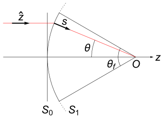
Figure 5: A schematic picture of focusing optics. The red line follows the photon beam. The incident plane wave along $z$-axis entering the plane $S_{0}$ is converted into the spherical wave with the unit vector $\mathbf{s}$ perpendicular to the sphere $S_{1}$, which is measured by the angle $\theta$ from the $z$-axis, and focused on the origin $O$. Here $\theta_{f}$ is the aperture angle.

Writing the electromagnetic field of the focused photon beam with the frequency $\omega$ as

$$\begin{split}\mathbf{E}(\mathbf{r},t)&=\frac{1}{2}\hat{\mathbf{E}}(\mathbf{r})e^{-\omega t}+c.c.\\ \mathbf{B}(\mathbf{r},t)&=\frac{1}{2}\hat{\mathbf{B}}(\mathbf{r})e^{-\omega t}+c.c.\,,\end{split}$$ (20)

we pay attention to the complex amplitudes $\hat{\mathbf{E}}(\mathbf{r})$ and $\hat{\mathbf{B}}(\mathbf{r})$. Eq. (19) allows us to express the amplitude of the electric field $\hat{\mathbf{E}}(\mathbf{r})$ as

$$\begin{split}\hat{\mathbf{E}}(\mathbf{r})&=\int^{\infty}_{-\infty}\int^{\infty}_{-\infty}ds_{x}ds_{y}\left[\mathbf{U}(s_{x},s_{y})e^{iks_{z}z}\right.\\ &\qquad\left.+\mathbf{V}(s_{x},s_{y})e^{-iks_{z}z}\right]e^{ik\left(s_{x}x+s_{y}y\right)}\,,\end{split}$$ (21)

where $s_{z}=\sqrt{1-s^{2}_{x}-s^{2}_{y}}$. Considering the case where $s^{2}_{x}+s^{2}_{y}\leq 1$, we find

$$\begin{split}\hat{\mathbf{E}}(\mathbf{r})&=\iint_{s^{2}_{x}+s^{2}_{y}\leq 1}ds_{x}ds_{y}\left[\mathbf{U}(s_{x},s_{y})e^{iks_{z}z}\right.\\ &\qquad\left.+\mathbf{V}(s_{x},s_{y})e^{-iks_{z}z}\right]e^{ik\left(s_{x}x+s_{y}y\right)}\,.\end{split}$$ (22)

By introducing the variables,

$$u_{x}=\frac{x}{f}\,,\ u_{y}=\frac{y}{f}\,,\ u_{z}=\frac{z}{f}=-\sqrt{1-u^{2}_{x}-u^{2}_{y}}\,,$$ (23)

$\hat{\mathbf{E}}(\mathbf{r})$ at a point $\mathbf{r}_{1}=(x_{1},y_{1},z_{1})$ on the sphere $S_{1}$ is evaluated as

$$\begin{split}\hat{\mathbf{E}}(\mathbf{r}_{1})&=\iint_{s^{2}_{x}+s^{2}_{y}\leq 1}ds_{x}ds_{y}\left[\mathbf{U}(s_{x},s_{y})e^{ikf\Phi_{+}(s_{x},s_{y})}\right.\\ &\qquad\left.+\mathbf{V}(s_{x},s_{y})e^{-ikf\Phi_{-}(s_{x},s_{y})}\right]\,,\end{split}$$ (24)

where $f$ stands for the focal distance, and

$$\Phi_{\pm}(s_{x},s_{y})=s_{x}x+s_{y}y\pm\sqrt{1-s^{2}_{x}-s^{2}_{y}}u_{z}\,.$$ (25)

Assuming the focal distance is larger than the wave length $fk\gg 1$, we apply the stationary phase method in evaluating the integration in Eq. (24). We first consider the first term in Eq. (24), to find that a stationary point $(s_{x_{0}},s_{y_{0}})$ satisfies

$$\begin{split}\frac{\partial\Phi_{+}(s_{x},s_{y})}{\partial s_{x}}&=u_{x}-\frac{s_{x}}{\sqrt{1-s^{2}_{x}-s^{2}_{y}}}u_{z}=0\,,\\ \frac{\partial\Phi_{+}(s_{x},s_{y})}{\partial s_{y}}&=u_{y}-\frac{s_{y}}{\sqrt{1-s^{2}_{x}-s^{2}_{y}}}u_{z}=0\,.\end{split}$$ (26)

Because $s_{x_{0}}<0$, one finds

$$s_{x_{0}}=-u_{x}\,,\ s_{y_{0}}=-u_{y}\,.$$ (27)

The Taylor expansion of $\Phi_{+}(s_{x},s_{y})$ around the stationary point $(s_{x_{0}},s_{y_{0}})$ gives

$$\begin{split}&\Phi_{+}(s_{x},s_{y})\\ &=\Phi_{+}(s_{x_{0}},s_{y_{0}})+\frac{w_{1}}{2}(s_{x}-s_{x_{0}})^{2}\\ &\quad+\frac{w_{2}}{2}(s_{y}-s_{y_{0}})^{2}+w_{3}(s_{x}-s_{x_{0}})(s_{y}-s_{y_{0}})+\cdots\,,\end{split}$$ (28)

where we have defined

$$\begin{split}w_{1}&=-\frac{1-u^{2}_{y}}{\left(1-s^{2}_{x}-s^{2}_{y}\right)^{3/2}}u_{z}\,,\\ w_{2}&=-\frac{1-u^{2}_{x}}{\left(1-s^{2}_{x}-s^{2}_{y}\right)^{3/2}}u_{z}\,,\\ w_{3}&=-\frac{u_{x}u_{y}}{\left(1-s^{2}_{x}-s^{2}_{y}\right)^{3/2}}u_{z}\,,\end{split}$$ (29)

with $u_{z}<0$, $w_{1}>0$, and $w_{2}>0$.

When $kf\gg 1$, the integrand in the vicinity of the stationary point $(s_{x_{0}},s_{y_{0}})$ mainly contributes to the integration, and thus, we find

$$\begin{split}&\mathbf{W}_{1}(\mathbf{r}_{1})\\ &\equiv\iint_{s^{2}_{x}+s^{2}_{y}\leq 1}ds_{x}ds_{y}\mathbf{U}(s_{x},s_{y})e^{ikf\Phi_{+}(s_{x},s_{y})}\\ &\approx\mathbf{U}(s_{x_{0}},s_{y_{0}})e^{ikf\Phi_{+}(s_{x_{0}},s_{y_{0}})}\iint_{s^{2}_{x}+s^{2}_{y}\leq 1}ds_{x}ds_{y}\\ &\quad e^{ikf\left[\frac{w_{1}}{2}(s_{x}-s_{x_{0}})^{2}+\frac{w_{2}}{2}(s_{y}-s_{y_{0}})^{2}+w_{3}(s_{x}-s_{x_{0}})(s_{y}-s_{y_{0}})\right]}\,.\end{split}$$ (30)

The infinitesimal region $(s_{x}-s_{x_{0}})^{2}+(s_{y}-s_{y_{0}})^{2}\leq\epsilon\ll 1$ dominates over the target integration domain $s^{2}_{x}+s^{2}_{y}\leq 1$. Defining $\epsilon_{x}\equiv s_{x}-s_{x_{0}}$ and $\epsilon_{y}\equiv s_{y}-s_{y_{0}}$, we find

$$\begin{split}&\mathbf{W}_{1}(\mathbf{r}_{1})\\ &=\mathbf{U}(s_{x_{0}},s_{y_{0}})e^{ikf\Phi_{+}(s_{x_{0}},s_{y_{0}})}\\ &\qquad\times\iint_{\epsilon^{2}_{x}+\epsilon^{2}_{y}\leq\epsilon}d\epsilon_{x}d\epsilon_{y}e^{ikf\left[\frac{w_{1}}{2}\epsilon^{2}_{x}+\frac{w_{2}}{2}\epsilon^{2}_{y}+w_{3}\epsilon_{x}\epsilon_{y}\right]}\\ &\approx\mathbf{U}(s_{x_{0}},s_{y_{0}})e^{ikf\Phi_{+}(s_{x_{0}},s_{y_{0}})}\\ &\quad\times\int^{\epsilon}_{-\epsilon}d\epsilon_{y}\int^{\sqrt{\epsilon^{2}-\epsilon^{2}_{y}}}_{-\sqrt{\epsilon^{2}-\epsilon^{2}_{y}}}d\epsilon_{x}e^{ikf\left[\frac{w_{1}}{2}\epsilon^{2}_{x}+\frac{w_{2}}{2}\epsilon^{2}_{y}+w_{3}\epsilon_{x}\epsilon_{y}\right]}\,.\end{split}$$ (31)

Performing change of variables, $X\equiv\sqrt{kf}\epsilon_{x}$ and $Y\equiv\sqrt{kf}\epsilon_{y}$, the integration can be approximated as

$$\begin{split}&\mathbf{W}_{1}(\mathbf{r}_{1})\\ &\approx\mathbf{U}(s_{x_{0}},s_{y_{0}})e^{ikf\Phi_{+}(s_{x_{0}},s_{y_{0}})}\\ &\quad\times\frac{1}{kf}\int^{\infty}_{-\infty}dY\int^{\infty}_{-\infty}dXe^{i\left[\frac{w_{1}}{2}X^{2}+\frac{w_{2}}{2}Y^{2}+w_{3}XY\right]}\,.\end{split}$$ (32)

Noting

$$\int^{\infty}_{-\infty}dY\int^{\infty}_{-\infty}dXe^{i\left[\frac{w_{1}}{2}X^{2}+\frac{w_{2}}{2}Y^{2}+w_{3}XY\right]}=-2\pi iu_{z}\,,$$ (33)

and using $\Phi_{+}(s_{x_{0}},s_{y_{0}})=-1$, we find

$$\mathbf{W}_{1}(\mathbf{r}_{1}) \approx-\frac{2\pi iu_{z}}{kf}U(-u_{x},-u_{y})e^{-ikf}\,.$$ (34)

In the same way, we can compute the second term in Eq. (24). Thus we find

$$\hat{\mathbf{E}}(\mathbf{r}_{1})\approx\frac{2\pi iu_{z}}{kf}\left[-\mathbf{U}(-u_{x},-u_{y})e^{-ikf}+\mathbf{V}(u_{x},u_{y})e^{ikf}\right]\,.$$ (35)

If there is no aberration in the focusing optics so that

$$\begin{split}s_{x}&=-\frac{x_{1}}{f}=-u_{x}\,,\\ s_{x}&=-\frac{y_{1}}{f}=-u_{y}\,,\\ s_{x}&=-\frac{z_{1}}{f}=-u_{z}\,,\end{split}$$ (36)

then we have

$$\hat{\mathbf{E}}(\mathbf{r}_{1})\approx\frac{2\pi is_{z}}{kf}\left[-\mathbf{U}(s_{x},s_{y})e^{-ikf}+\mathbf{V}(-s_{x},-s_{y})e^{ikf}\right]\,.$$ (37)

Next, we compute the coefficients $U(s_{x},s_{y})$ and $V(-s_{x},-s_{y})$ in Eq. (37). Because the amplitude of the spherical wave is proportional to the inverse of distance, we can express $\hat{E}(\mathbf{r}_{1})$ as

$$\hat{\mathbf{E}}(\mathbf{r}_{1})=\frac{{\bf a}_{1}(s_{x},s_{y})}{f}e^{ik\phi(\mathbf{r}_{1})}\,.$$ (38)

Here, $\mathbf{a}_{1}(s_{x},s_{y})$ is a vector perpendicular to the light ray from the sphere $S_{1}$ to the focus $O$, and $\phi(\mathbf{r}_{1})$ is the eikonal function to describe the optical path length from a point $O^{\prime}$ to $\mathbf{r}_{1}$ in the object space. Assuming the optical path length of the spherical wave with its source at point $O^{\prime}$ which converges at the focus $O$ through the point $\mathbf{r}_{1}$ is expressed by the constant $C$ to be

$$\phi(\mathbf{r}_{1})=C-|\mathbf{r}_{1}|=C-f\,.$$ (39)

Thus, we find the relation between ${\bf a}_{1}(s_{x},s_{y})$ and the coefficients $\mathbf{U}(s_{x},s_{y})$, $\mathbf{V}(-s_{x},-s_{y})$ as follows

$$\begin{split}\mathbf{U}(s_{x},s_{y})&=-\frac{ik}{2\pi}\frac{\mathbf{a}_{1}(s_{x},s_{y})}{s_{z}}e^{ikC}\ \\ \mathbf{V}(s_{x},s_{y})&=0\,.\end{split}$$ (40)

Ignoring the constant factor $e^{ikC}$ and substituting the above into Eq. (22), we obtain the amplitude of the electric field,

$$\hat{\mathbf{E}}(\mathbf{r})=-\frac{ik}{2\pi}\iint_{s^{2}_{x}+s^{2}_{y}\leq 1}ds_{x}ds_{y}\frac{\mathbf{a}_{1}(s_{x},s_{y})}{s_{z}}e^{ik\mathbf{s}\cdot\mathbf{r}}\,,$$ (41)

and, in a similar way, that of the magnetic field goes like

$$\hat{\mathbf{B}}(\mathbf{r})=-\frac{ik}{2\pi}\iint_{s^{2}_{x}+s^{2}_{y}\leq 1}ds_{x}ds_{y}\frac{\mathbf{a}_{2}(s_{x},s_{y})}{s_{z}}e^{ik\mathbf{s}\cdot\mathbf{r}}\,.$$ (42)

Finally, we rewrite ${\bf a}_{1}(s_{x},s_{y})$ and ${\bf a}_{2}(s_{x},s_{y})$ in terms of angles in the polar coordinate. Considering $\mathbf{e}_{0}(\theta,\varphi)$ as the electric field (with the phase removed) of the incident light ray on the plane $S_{0}$ and $\mathbf{e}_{1}(\theta,\varphi)$ as that on the sphere $S_{1}$, we write $\hat{\mathbf{e}}_{0}(\varphi)$ and $\hat{\mathbf{e}}_{1}(\theta,\varphi)$ as unit vectors parallel to $\mathbf{e}_{0}(\theta,\varphi)$ and $\mathbf{e}_{1}(\theta,\varphi)$, respectively. One then finds

$$\mathbf{e}_{1}(\theta,\varphi)=\frac{\mathbf{a}_{1}(\theta,\varphi)}{f}\,.$$ (43)

Let $\delta S_{0}$ be the infinitesimal circular ring on $S_{0}$, and $\delta S_{1}$ be the area of the projection of $\delta S_{0}$ onto $S_{1}$. Then the following relation holds between $\delta S_{0}$ and $\delta S_{1}$:

$$\delta S_{0}=\delta S_{1}\cos\theta\,.$$ (44)

Using the energy conservation law

$$|\mathbf{e}_{0}(\theta,\varphi)|^{2}\delta S_{0}=|\mathbf{e}_{1}(\theta,\varphi)|^{2}\delta S_{1}\,,$$ (45)

we obtain

$$\mathbf{e}_{1}(\theta,\varphi)=|\mathbf{e}_{0}(\theta,\varphi)|\cos^{\frac{1}{2}}\theta\,\hat{\mathbf{e}}_{1}(\theta,\varphi)\,.$$ (46)

Let the two vectors $\mathbf{g}_{0}(\varphi)$ and $\mathbf{g}_{1}(\theta,\varphi)$ be unit vectors, that are perpendicular to the incident light ray and the focused light ray, respectively. They lie on a plane including both the light ray and the optical axis (see Fig. 6).

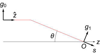
Figure 6: Alignment of vectors and coordinate system. The detailed description is provided in the text.

$\mathbf{g}_{0}(\varphi)$ and $\mathbf{g}_{1}(\theta,\varphi)$ are given as

$$\begin{split}\mathbf{g}_{0}(\varphi)&=\cos\varphi\,\hat{\mathbf{x}}+\sin\varphi\,\hat{\mathbf{y}}\\ \mathbf{g}_{1}(\theta,\varphi)&=\cos\theta\cos\varphi\,\hat{\mathbf{x}}+\cos\theta\sin\varphi\,\hat{\mathbf{y}}+\sin\theta\,\hat{\mathbf{z}}\\ \mathbf{s}(\theta,\varphi)&=-\sin\theta\cos\varphi\,\hat{\mathbf{x}}-\sin\theta\sin\varphi\,\hat{\mathbf{y}}+\cos\theta\,\hat{\mathbf{z}}\,,\end{split}$$ (47)

where $\hat{\mathbf{x}}$, $\hat{\mathbf{y}}$, and $\hat{\mathbf{z}}$ are $x,y,z$-direction unit vectors. By definition, we have

$$\begin{split}\mathbf{g}_{0}(\varphi)\times\hat{\mathbf{z}}&=\mathbf{g}_{1}(\theta,\varphi)\times\mathbf{s}(\theta,\varphi)\\ &=\sin\varphi\,\hat{\mathbf{x}}-\cos\varphi\,\hat{\mathbf{y}}\,.\end{split}$$ (48)

Because $\hat{\mathbf{e}}_{0}(\varphi)$ is perpendicular to the $z$-axis, we can decompose it as

$$\begin{split}\hat{\mathbf{e}}_{0}(\varphi)&=\left[\hat{\mathbf{e}}_{0}(\varphi)\cdot\mathbf{g}_{0}(\varphi)\right]\mathbf{g}_{0}(\varphi)\\ &\qquad+\left[\hat{\mathbf{e}}_{0}(\varphi)\cdot\left(\mathbf{g}_{0}(\varphi)\times\hat{\mathbf{z}}\right)\right]\left(\mathbf{g}_{0}(\varphi)\times\hat{\mathbf{z}}\right)\,.\end{split}$$ (49)

When $\mathbf{e}_{0}(\theta,\varphi)$ is converted into $\mathbf{e}_{1}(\theta,\varphi)$, the $\mathbf{g}_{0}(\varphi)$-direction component is transformed into the $\mathbf{g}_{1}(\varphi)$-direction component, and the $\mathbf{g}_{0}(\varphi)\times\hat{\mathbf{z}}$-direction component is done into the $\mathbf{g}_{1}(\theta,\varphi)\times\mathbf{s}(\theta,\varphi)$-direction component. Thus,

$$\begin{split}&\mathbf{e}_{1}(\theta,\varphi)\\ &=|\mathbf{e}_{0}(\theta,\varphi)|\cos^{\frac{1}{2}}\theta\left\{\left[\hat{\mathbf{e}}_{0}(\varphi)\cdot\mathbf{g}_{0}(\varphi)\right]\mathbf{g}_{1}(\varphi)\right.\\ &\qquad\left.+\left[\hat{\mathbf{e}}_{0}(\varphi)\cdot(\mathbf{g}_{0}(\varphi)\times\hat{\mathbf{z}})\right]\left(\mathbf{g}_{1}(\theta,\varphi)\times\mathbf{s}(\theta,\varphi)\right)\right\}\,.\end{split}$$ (50)

In the focusing optics without aberration, we can express $\mathbf{e}_{0}(\theta,\varphi)$ as

$$\mathbf{e}_{0}(\theta,\varphi)=e_{0}l_{0}(\theta)\hat{\mathbf{e}}_{0}(\varphi)\,,$$ (51)

where $e_{0}$ is the maximum value of $|\mathbf{e}_{0}(\theta,\varphi)|$, and $l_{0}(\theta)$ is the relative amplitude. Therefore, by using Eq. (43), we obtain

$$\begin{split}&\mathbf{a}_{1}(\theta,\varphi)\\ &=fe_{0}l_{0}(\theta)\cos^{\frac{1}{2}}\theta\left\{\left[\hat{\mathbf{e}}_{0}(\varphi)\cdot\mathbf{g}_{0}(\varphi)\right]\mathbf{g}_{1}(\theta,\varphi)\right.\\ &\qquad\left.+\left[\hat{\mathbf{e}}_{0}(\varphi)\cdot(\mathbf{g}_{0}(\varphi)\times\hat{\mathbf{z}})\right]\left(\mathbf{g}_{1}(\theta,\varphi)\times\mathbf{s}(\theta,\varphi)\right)\right\}\,.\end{split}$$ (52)

The relation between the electric and magnetic fields leads to

$$\begin{split}&\mathbf{a}_{2}(\theta,\varphi)\\ &=\mathbf{s}(\theta,\varphi)\times\mathbf{a}_{1}(\theta,\varphi)\\ &=fe_{0}l_{0}(\theta)\cos^{\frac{1}{2}}\theta\left\{\left[\hat{\mathbf{e}}_{0}(\varphi)\cdot(\mathbf{g}_{0}(\varphi)\times\hat{\mathbf{z}})\right]\mathbf{g}_{1}(\theta,\varphi)\right.\\ &\qquad\left.-\left[\hat{\mathbf{e}}_{0}(\varphi)\cdot\mathbf{g}_{0}(\varphi)\right]\left(\mathbf{g}_{1}(\theta,\varphi)\times\mathbf{s}(\theta,\varphi)\right)\right\}\,.\end{split}$$ (53)

In the cylindrical coordinate $(\rho,\varphi,z)$, $\mathbf{r}=\rho\cos\varphi\,\hat{\mathbf{x}}+\rho\sin\varphi\,\hat{\mathbf{y}}+z\,\hat{\mathbf{z}}$, and Eq. (47) tells us

$$\mathbf{s}(\theta^{\prime},\varphi^{\prime})\cdot\mathbf{r} =z\cos\theta^{\prime}-\rho\sin\theta^{\prime}\cos\left(\varphi^{\prime}-\varphi\right)\,.$$ (54)

The Jacobian goes like

$$\frac{\partial\left(s_{x},s_{y}\right)}{\partial\left(\theta^{\prime},\varphi^{\prime}\right)}=\sin\theta^{\prime}\cos\theta^{\prime}\,,\ ds_{x}ds_{y}=s_{z}\sin\theta^{\prime}d\theta^{\prime}d\varphi^{\prime}\,.$$ (55)

Thus Eqs. (41) and (42) are written in the polar-coordinate as follows:

$$\begin{split}\hat{\mathbf{E}}(\mathbf{r})&=-\frac{ik}{2\pi}\int^{\frac{\theta_{f}}{2}}_{0}d\theta^{\prime}\int^{2\pi}_{0}d\varphi^{\prime}\mathbf{a}_{1}(\theta^{\prime},\varphi^{\prime})\sin\theta^{\prime}\\ &\qquad\qquad\qquad\qquad e^{ik\left[z\cos\theta^{\prime}-\rho\sin\theta^{\prime}\cos\left(\varphi^{\prime}-\varphi\right)\right]}\,,\end{split}$$ (56)

$$\begin{split}\hat{\mathbf{B}}(\mathbf{r})&=-\frac{ik}{2\pi}\int^{\frac{\theta_{f}}{2}}_{0}d\theta^{\prime}\int^{2\pi}_{0}d\varphi^{\prime}\mathbf{a}_{2}(\theta^{\prime},\varphi^{\prime})\sin\theta^{\prime}\\ &\qquad\qquad\qquad\qquad e^{ik\left[z\cos\theta^{\prime}-\rho\sin\theta^{\prime}\cos\left(\varphi^{\prime}-\varphi\right)\right]}\,.\end{split}$$ (57)

A.2 Linear Polarization

When the incident photon beam is linearly polarized, Eq. (51) goes like

$$\mathbf{e}_{0}(\theta,\varphi)=e_{0}l_{g}(\theta)\hat{\mathbf{x}}\,,\ \hat{\mathbf{e}}_{0}(\varphi)=\hat{\mathbf{x}}\,,$$ (58)

where $l_{g}(\theta)$ expresses the Gaussian distribution,

$$l_{g}(\theta)=\exp\left[-\left(\frac{\sin\theta}{\sin\frac{\theta_{f}}{2}}\right)^{2}\right]\,.$$ (59)

Using

$$\begin{split}\hat{\mathbf{e}}_{0}(\varphi)\cdot\mathbf{g}_{0}(\varphi)&=\cos\varphi\,,\\ \hat{\mathbf{e}}_{0}(\varphi)\cdot(\mathbf{g}_{0}(\varphi)\times\hat{\mathbf{z}})&=\sin\varphi\,,\end{split}$$ (60)

we can derive each component of $\mathbf{a}_{1}(\theta,\varphi)$ and $\mathbf{a}_{2}(\theta,\varphi)$ in the Cartesian coordinate as follows:

$$\begin{split}&\mathbf{a}_{1}(\theta,\varphi)\\ &=\frac{1}{2}fe_{0}l_{g}(\theta)\cos^{\frac{1}{2}}\theta\\ &\qquad\times\left\{\left[(1+\cos\theta)-(1-\cos\theta)\cos 2\varphi\right]\hat{\mathbf{x}}\right.\\ &\qquad\qquad\left.+(\cos\theta-1)\sin 2\varphi\,\hat{\mathbf{y}}+2\sin\theta\cos\varphi\,\hat{\mathbf{z}}\right\}\,,\end{split}$$ (61)

$$\begin{split}&\mathbf{a}_{2}(\theta,\varphi)\\ &=\frac{1}{2}fe_{0}l_{g}(\theta)\cos^{\frac{1}{2}}\theta\\ &\qquad\times\left\{(\cos\theta-1)\sin 2\varphi\,\hat{\mathbf{x}}\right.\\ &\qquad\qquad+\left[\left(1+\cos\theta\right)+(1-\cos\theta)\cos 2\varphi\right]\hat{\mathbf{y}}\\ &\qquad\qquad\qquad\left.+2\sin\theta\sin\varphi\,\hat{\mathbf{z}}\right\}\,.\end{split}$$ (62)

Substituting the above into Eqs. (56) and (57), we finally obtain the amplitudes of the electric field and magnetic field as follows:

$$\begin{split}\hat{E}_{x}(\rho,\varphi,z)&=-iA\left[I_{0}(\rho,z)+\cos 2\varphi I_{2}(\rho,z)\right]\,,\\ \hat{E}_{y}(\rho,\varphi,z)&=-iA\sin 2\varphi I_{2}(\rho,z)\,,\\ \hat{E}_{z}(\rho,\varphi,z)&=-2A\cos\varphi I_{1}(\rho,z)\,,\\ \hat{B}_{x}(\rho,\varphi,z)&=-iA\sin 2\varphi I_{2}(\rho,z)\,,\\ \hat{B}_{y}(\rho,\varphi,z)&=-iA\left[I_{0}(\rho,z)-\cos 2\varphi I_{2}(\rho,z)\right]\,,\\ \hat{B}_{z}(\rho,\varphi,z)&=-2A\cos\varphi I_{1}(\rho,z)\,,\end{split}$$ (63)

where $A=kfe_{0}/2$, and

$$\begin{split}I_{0}(\rho,z)&=\int^{\frac{\theta_{f}}{2}}_{0}d\theta^{\prime}l_{g}(\theta^{\prime})\cos^{\frac{1}{2}}\theta^{\prime}\sin\theta^{\prime}\\ &\qquad\qquad\times(1+\cos\theta^{\prime})J_{0}(k\rho\sin\theta^{\prime})e^{ikz\cos\theta^{\prime}}\,,\\ I_{1}(\rho,z)&=\int^{\frac{\theta_{f}}{2}}_{0}d\theta^{\prime}l_{g}(\theta^{\prime})\cos^{\frac{1}{2}}\theta^{\prime}\sin^{2}\theta^{\prime}\,,\\ &\qquad\qquad\qquad\times J_{1}(k\rho\sin\theta^{\prime})e^{ikz\cos\theta^{\prime}}\\ I_{2}(\rho,z)&=\int^{\frac{\theta_{f}}{2}}_{0}d\theta^{\prime}l_{g}(\theta^{\prime})\cos^{\frac{1}{2}}\theta^{\prime}\sin\theta^{\prime}\\ &\qquad\qquad\times(1-\cos\theta^{\prime})J_{2}(k\rho\sin\theta^{\prime})e^{ikz\cos\theta^{\prime}}\,,\end{split}$$ (64)

where $J_{n}(x)\,(n=0,1,2)$ is Bessel function of the first kind.

A.3 Circular Polarization

When the incident photon beam is circularly polarized, Eq. (51) goes like

$$\begin{split}\mathbf{e}_{0}(\theta,\varphi)&=e_{0}l_{g}(\theta)\left(\cos\varphi_{0}\hat{\mathbf{\rho}}-\sin\varphi_{0}\hat{\mathbf{\varphi}}\right)\,,\\ \hat{\mathbf{e}}_{0}(\varphi)&=\left(\cos\varphi_{0}\hat{\bm{\rho}}-\sin\varphi_{0}\hat{\bm{\varphi}}\right)\,,\ \varphi_{0}=\frac{\pi}{4}\,,\end{split}$$ (65)

where $l_{bg}(\theta)$ expresses the Bessel-Gaussian distribution,

$$l_{bg}(\theta)=J_{1}\left(\frac{\sin\theta}{\sin\frac{\theta_{f}}{2}}\right)\exp\left[-\left(\frac{\sin\theta}{\sin\frac{\theta_{f}}{2}}\right)^{2}\right]\,.$$ (66)

Here, one finds

$$\hat{\bm{\rho}}=\cos\varphi\hat{\mathbf{x}}+\sin\varphi\hat{\mathbf{y}}\,,\hat{\bm{\varphi}}=-\sin\varphi\hat{\mathbf{x}}+\cos\varphi\hat{\mathbf{y}}\,.$$ (67)

In a way similar to the case of the linear polarization we thus get

$$\begin{split}\hat{E}_{x}(\rho,\varphi,z)&=-2A\left[\cos\varphi_{0}\cos\varphi U_{0}(\rho,z)\right.\,,\\ &\left.\qquad\qquad+\sin\varphi_{0}\sin\varphi U_{2}(\rho,z)\right]\,,\\ \hat{E}_{y}(\rho,\varphi,z)&=-2A\left[\cos\varphi_{0}\sin\varphi U_{0}(\rho,z)\right.\,,\\ &\left.\qquad\qquad-\sin\varphi_{0}\cos\varphi U_{2}(\rho,z)\right]\,,\\ \hat{E}_{z}(\rho,\varphi,z)&=-2iA\cos\varphi_{0}U_{1}(\rho,z)\,,\\ \hat{B}_{x}(\rho,\varphi,z)&=-2A\left[\sin\varphi_{0}\cos\varphi U_{0}(\rho,z)\right.\,,\\ &\left.\qquad\qquad-\cos\varphi_{0}\sin\varphi U_{2}(\rho,z)\right]\,,\\ \hat{B}_{y}(\rho,\varphi,z)&=-2A\left[\sin\varphi_{0}\sin\varphi U_{0}(\rho,z)\right.\,,\\ &\left.\qquad\qquad+\cos\varphi_{0}\cos\varphi U_{2}(\rho,z)\right]\,,\\ \hat{B}_{z}(\rho,\varphi,z)&=-2iA\sin\varphi_{0}U_{1}(\rho,z)\,,\end{split}$$ (68)

where

$$\begin{split}U_{0}(\rho,z)&=\int^{\frac{\theta_{f}}{2}}_{0}d\theta^{\prime}l_{bg}(\theta^{\prime})\cos^{\frac{3}{2}}\theta^{\prime}\sin\theta^{\prime}\\ &\qquad\qquad\qquad J_{1}(k\rho\sin\theta^{\prime})e^{ikz\cos\theta^{\prime}}\,,\\ U_{1}(\rho,z)&=\int^{\frac{\theta_{f}}{2}}_{0}d\theta^{\prime}l_{bg}(\theta^{\prime})\cos^{\frac{1}{2}}\theta^{\prime}\sin^{2}\theta^{\prime}\\ &\qquad\qquad\qquad J_{0}(k\rho\sin\theta^{\prime})e^{ikz\cos\theta^{\prime}}\,,\\ U_{2}(\rho,z)&=\int^{\frac{\theta_{f}}{2}}_{0}d\theta^{\prime}l_{bg}(\theta^{\prime})\cos^{\frac{1}{2}}\theta^{\prime}\sin\theta^{\prime}\\ &\qquad\qquad\qquad J_{1}(k\rho\sin\theta^{\prime})e^{ikz\cos\theta^{\prime}}\,.\end{split}$$ (69)

A.4 Amplitude distribution

We compute the amplitudes of electric field $\mathbf{E}$ and magnetic field $\mathbf{B}$ and evaluate the field-strength squared $F_{\mu\nu}F^{\mu\nu}$. In the following, we focus only on the root mean square of each quantity. That is,

$$\begin{split}\sqrt{\langle|\mathbf{E}(\mathbf{r},t)|^{2}\rangle}&=\frac{1}{\sqrt{2}}\sqrt{|\hat{\mathbf{E}}(\mathbf{r})|^{2}}\end{split}\,,$$ (70)

$$\begin{split}\sqrt{\langle|\mathbf{B}(\mathbf{r},t)|^{2}\rangle}&=\frac{1}{\sqrt{2}}\sqrt{|\hat{\mathbf{B}}(\mathbf{r})|^{2}}\end{split}\,,$$ (71)

$$\begin{split}\sqrt{\langle|F_{\mu\nu}F^{\mu\nu}(\mathbf{r},t)|^{2}\rangle}&=\frac{2}{\sqrt{2}}\sqrt{|\hat{\mathbf{B}}^{2}(\mathbf{r})-\hat{\mathbf{E}}^{2}(\mathbf{r})|^{2}}\,.\end{split}$$ (72)

Based on the experimental setup, we utilize the set of parameters in Table 1.

Parameters
Creation beam frequency	2.8 GHz
Inducing beam frequency	1.6 GHz
Creation beam diameter	6.02 m
Inducing beam diameter	6.10 m
Common focal length	30 m

Table 1: Experimental parameters for the stimulated radar collider setup, as listed in Homma and Kirita (2020).

From the geometrical parameters, we compute the aperture angle $\theta_{f}$ (see also Fig. 5),

$$\theta_{f}=2\arctan\left(\frac{\mbox{beam radius [m]}}{\mbox{focal length [m]}}\right)\,.$$ (73)

Hereafter, we use the parameters of creation beam in evaluating the amplitudes of the electric and magnetic fields. Furthermore, we normalize the amplitude of the electric field for the incident beam $e_{0}=1$, thus $A=kf/2$, to see how the electric and magnetic fields are amplified in the focused beam.

First, we consider the case of focusing the linearly polarized beam. We plot the amplitude distribution of the electric field, magnetic field, and field-strength squared on the focal plane ($z=0$) in Figs 7, 8, 9.

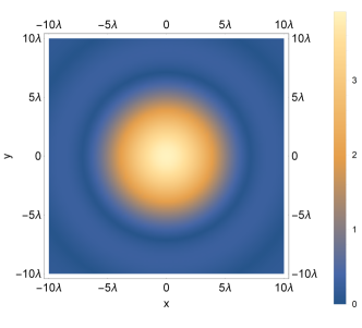
Figure 7: The root mean square of the electric field in linearly polarized beam, showing the amplitude distribution on the focal plane ($z=0$), where the center corresponds to the $z$-axis.

Figure 8: The same as Fig. 7, but for the magnetic field in linearly polarized beam.

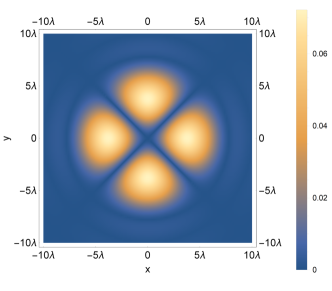
Figure 9: The same as Figs. 7 and 8, but for the field-strength squared in linearly polarized beam.

Note that $e^{ikz\cos\theta^{\prime}}$ in Eq. (64) vanishes on the focal plane. In each plot, the $(x,y)$ coordinate is in the unit of the wavelength $\lambda$ because the $\rho(x,y)$-dependence originates from $J_{n}(k\rho\sin\theta^{\prime})$ and $k\rho=2\pi\rho/\lambda$. One finds that the amplitude distributions of the electric and magnetic fields are elliptical for the linearly polarized beam. The plot of the amplitude distribution shows that the field-strength squared vanishes on $z$-axis ($\rho=0$) of the focal plane for the linearly polarized beam.

Next, we consider the case of focusing the circularly polarized beam. We plot the amplitude distribution of the electric field and magnetic field in Figs 10, 11. Equation (69) shows that $U_{0}$ and $U_{2}$ vanishes when $\rho\rightarrow 0$, and only $\hat{E}_{z}$ and $\hat{B}_{z}$ on $z$-axis ($\rho=0$) contributes to the total amplitudes. From Eq. (68), one finds that the electric and magnetic fields have the same amplitude at each point on the focal plane for the circularly polarized beam ($\varphi_{0}=\pi/4$). Therefore, the field-strength square vanishes on the focal plane for the circularly polarized beam.

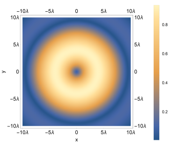
Figure 10: The root mean square of the electric field in circularly polarized beam.

Figure 11: The root mean square of the magnetic field in circularly polarized beam.

Appendix B Dark Energy Models of $F(R)$ Gravity

We briefly review two cosmological models of $F(R)$ gravity: Starobinsky Starobinsky (2007) model and Hu-Sawicki model Hu and Sawicki (2007), which have been widely used in the study on late-time cosmology. First, the Starobinsky model is describe by the following $F(R)$ function:

$$F_{\mathrm{S}}(R)=R-\mu_{\mathrm{S}}R_{\mathrm{S}}\left[1-\left(1+\frac{R^{2}}{R^{2}_{\mathrm{S}}}\right)^{-l}\right]\,.$$ (74)

$R_{\mathrm{S}}$ represents a background curvature of the DE vacuum, $\mu_{\mathrm{S}}$ and $l$ are positive parameters. In the large-curvature limit $R\gg R_{S}$, the Starobinsky model approximates to

$$F_{S}(R) \approx R-\mu_{\mathrm{S}}R_{\mathrm{S}}\left[1-\left(\frac{R}{R_{\mathrm{S}}}\right)^{-2l}\right]$$

$$=R-\mu_{\mathrm{S}}R_{\mathrm{S}}+\mu_{\mathrm{S}}R_{\mathrm{S}}\left(\frac{R}{R_{\mathrm{S}}}\right)^{-2l}\,.$$ (75)

The second term in the second line can be considered as the cosmological constant, $\mu_{S}R_{S}=2\Lambda$.

Second, the $F(R)$ function for the Hu-Sawicki model is:

$$F_{\mathrm{HS}}(R)=R-R_{\mathrm{HS}}\frac{c_{1}\left(\frac{R}{R_{\mathrm{HS}}}\right)^{m}}{1+c_{2}\left(\frac{R}{R_{\mathrm{HS}}}\right)^{m}}\,,$$ (76)

$R_{HS}$ represents the background curvature of the DE vacuum in this model, $c_{1}$, $c_{2}$, and $m$ are positive parameters. Here, we consider to change the parametrization for this $F_{\rm HS}(R)$ as follows:

$$F_{\mathrm{HS}}(R)=R-\mu_{\mathrm{HS}}\tilde{R}_{\mathrm{HS}}\frac{\left(\frac{R}{\tilde{R}_{\mathrm{HS}}}\right)^{m}}{1+\left(\frac{R}{\tilde{R}_{\mathrm{HS}}}\right)^{m}}\,,$$ (77)

where $\mu_{HS}=\frac{c_{1}}{c^{1-1/m}_{2}}$ and $\tilde{R}_{\mathrm{HS}}=\frac{R_{\mathrm{HS}}}{c^{1/m}_{2}}$. In the large-curvature limit $R\gg\tilde{R}_{\mathrm{HS}}$, the Hu-Sawicki model approximates to

$$F_{\mathrm{HS}}(R) \approx R-\mu_{HS}\tilde{R}_{HS}\left[1-\left(\frac{R}{\tilde{R}_{HS}}\right)^{-m}\right]$$

$$=R-\mu_{\mathrm{HS}}\tilde{R}_{\mathrm{HS}}+\mu_{\mathrm{HS}}\tilde{R}_{\mathrm{HS}}\left(\frac{R}{\tilde{R}_{\mathrm{HS}}}\right)^{-m}\,.$$ (78)

In a way similar to the case of the Starobinsky model, the second term in the second line can be considered as the cosmological constant, $\mu_{S}\tilde{R}_{S}=\frac{c_{1}}{c_{2}}R_{\mathrm{HS}}=2\Lambda$.

Therefore, those two models are reduced to the same form of $F(R)$ gravity in the large-curvature limit as follows:

$$F(R)=R-\lambda R_{c}\left[1-\left(\frac{R}{R_{c}}\right)^{-2n}\right]$$ (79)

Correspondence of parameters to those in Starobinsky and Hu-Sawicki models reads

$$R_{c} =R_{S}\,,\ \lambda=\mu_{S}\,,\ n=l$$ (80)

$$R_{c} =\frac{R_{HS}}{c^{1/m}_{2}}\,,\ \lambda=\frac{c_{1}}{c^{1-1/m}_{2}}\,,\ n=\frac{m}{2}\,.$$ (81)

Note that when we take the limit $\mu\rightarrow\infty$ and $R_{c}\rightarrow 0$ with fixing $\mu R_{c}$, we obtain the general relativity with the cosmological constant, that is, $\Lambda$-CDM model.

Appendix C Evaluation of Gas in Chamber

The specific gas constants for typical residual gases are shown in Table 2.

Gas	Molar mass [kg/mol]	$\mathcal{R}$
Hydrogen ($\mathrm{H_{2}}$)	$2.0159\times 10^{-3}$	4124
Water vapor ($\mathrm{H_{2}O}$)	$18.015\times 10^{-3}$	461.5
Nitrogen ($\mathrm{N_{2}}$)	$28.013\times 10^{-3}$	296.8
Carbon Monoxide ($\mathrm{CO}$)	$28.010\times 10^{-3}$	296.8
Dry air (mixture)	$28.965\times 10^{-3}$	287.1
Carbon Dioxide ($\mathrm{CO_{2}}$)	$44.010\times 10^{-3}$	188.9

Table 2: Specific gas constant for several gas species.

As an illustration, we consider the dry air. For the room temperature $T=300~{}[\mathrm{K}]$ and the pressure $P=10^{-7}~{}[\mathrm{Pa}]$, we find $\rho=1.16\times 10^{-12}~{}[\mathrm{kg/m^{3}}]$. Note that $1~{}[\mathrm{Pa}]=4.80\times 10^{-2}~{}[\mathrm{eV^{4}}]$ and $1~{}[\mathrm{kg/m^{3}}]=4.31\times 10^{15}~{}[\mathrm{eV^{4}}]$, and thus, $P=4.80\times 10^{-9}~{}[\mathrm{eV^{4}}]$ and $\rho=5.00\times 10^{3}~{}[\mathrm{eV^{4}}]$. Then, we can ignore the pressure in evaluating the trace of the energy-momentum tensor, thus, $T^{\mu}_{\ \mu(\mathrm{gas})}\approx-\rho$.

References

- Caldwell et al. (1998) R. Caldwell, R. Dave, and P. J. Steinhardt, Phys. Rev. Lett. 80, 1582 (1998), arXiv:astro-ph/9708069 .
- Peebles and Ratra (2003) P. Peebles and B. Ratra, Rev. Mod. Phys. 75, 559 (2003), arXiv:astro-ph/0207347 .
- Copeland et al. (2006) E. J. Copeland, M. Sami, and S. Tsujikawa, Int. J. Mod. Phys. D 15, 1753 (2006), arXiv:hep-th/0603057 .
- Will (2014) C. M. Will, Living Rev. Rel. 17, 4 (2014), arXiv:1403.7377 [gr-qc] .
- Adelberger et al. (2003) E. Adelberger, B. R. Heckel, and A. Nelson, Ann. Rev. Nucl. Part. Sci. 53, 77 (2003), arXiv:hep-ph/0307284 .
- Spero et al. (1980) R. Spero, J. Hoskins, R. Newman, J. Pellam, and J. Schultz, Phys. Rev. Lett. 44, 1645 (1980).
- Kapner et al. (2007) D. Kapner, T. Cook, E. Adelberger, J. Gundlach, B. R. Heckel, C. Hoyle, and H. Swanson, Phys. Rev. Lett. 98, 021101 (2007), arXiv:hep-ph/0611184 .
- Marion et al. (2003) H. Marion et al., Phys. Rev. Lett. 90, 150801 (2003), arXiv:physics/0212112 .
- Peik et al. (2004) E. Peik, B. Lipphardt, H. Schnatz, T. Schneider, C. Tamm, and S. G. Karshenboim, Phys. Rev. Lett. 93, 170801 (2004), arXiv:physics/0402132 .
- Damour and Dyson (1996) T. Damour and F. Dyson, Nucl. Phys. B 480, 37 (1996), arXiv:hep-ph/9606486 .
- Srianand et al. (2004) R. Srianand, H. Chand, P. Petitjean, and B. Aracil, Phys. Rev. Lett. 92, 121302 (2004), arXiv:astro-ph/0402177 .
- De Felice and Tsujikawa (2010) A. De Felice and S. Tsujikawa, Living Rev. Rel. 13, 3 (2010), arXiv:1002.4928 [gr-qc] .
- Nojiri and Odintsov (2011) S. Nojiri and S. D. Odintsov, Phys. Rept. 505, 59 (2011), arXiv:1011.0544 [gr-qc] .
- Clifton et al. (2012) T. Clifton, P. G. Ferreira, A. Padilla, and C. Skordis, Phys. Rept. 513, 1 (2012), arXiv:1106.2476 [astro-ph.CO] .
- Capozziello and De Laurentis (2011) S. Capozziello and M. De Laurentis, Phys. Rept. 509, 167 (2011), arXiv:1108.6266 [gr-qc] .
- Nojiri et al. (2017) S. Nojiri, S. D. Odintsov, and V. K. Oikonomou, Phys. Rept. 692, 1 (2017), arXiv:1705.11098 [gr-qc] .
- Khoury and Weltman (2004) J. Khoury and A. Weltman, Phys. Rev. Lett. 93, 171104 (2004), arXiv:astro-ph/0309300 .
- Burrage and Sakstein (2018) C. Burrage and J. Sakstein, Living Rev. Rel. 21, 1 (2018), arXiv:1709.09071 [astro-ph.CO] .
- Chou et al. (2009) A. S. Chou et al. (GammeV), Phys. Rev. Lett. 102, 030402 (2009), arXiv:0806.2438 [hep-ex] .
- Steffen et al. (2010) J. H. Steffen, A. Upadhye, A. Baumbaugh, A. S. Chou, P. O. Mazur, R. Tomlin, A. Weltman, and W. Wester (GammeV), Phys. Rev. Lett. 105, 261803 (2010), arXiv:1010.0988 [astro-ph.CO] .
- Rybka et al. (2010) G. Rybka et al. (ADMX), Phys. Rev. Lett. 105, 051801 (2010), arXiv:1004.5160 [astro-ph.CO] .
- Brax et al. (2009) P. Brax, C. Burrage, A.-C. Davis, D. Seery, and A. Weltman, JHEP 09, 128 (2009), arXiv:0904.3002 [hep-ph] .
- Anastassopoulos et al. (2019) V. Anastassopoulos et al. (CAST), JCAP 01, 032 (2019), arXiv:1808.00066 [hep-ex] .
- Levshakov et al. (2010) S. A. Levshakov, P. Molaro, A. V. Lapinov, D. Reimers, C. Henkel, and T. Sakai, Astron. Astrophys. 512, A44 (2010), arXiv:0911.3732 [astro-ph.CO] .
- Vagnozzi et al. (2021) S. Vagnozzi, L. Visinelli, P. Brax, A.-C. Davis, and J. Sakstein, Phys. Rev. D 104, 063023 (2021), arXiv:2103.15834 [hep-ph] .
- Homma and Kirita (2020) K. Homma and Y. Kirita, JHEP 09, 095 (2020), arXiv:1909.00983 [hep-ex] .
- Nunes et al. (2017) R. C. Nunes, S. Pan, E. N. Saridakis, and E. M. C. Abreu, JCAP 01, 005 (2017), arXiv:1610.07518 [astro-ph.CO] .
- Starobinsky (2007) A. A. Starobinsky, JETP Lett. 86, 157 (2007), arXiv:0706.2041 [astro-ph] .
- Hu and Sawicki (2007) W. Hu and I. Sawicki, Phys. Rev. D76, 064004 (2007), arXiv:0705.1158 [astro-ph] .
- Katsuragawa et al. (2019) T. Katsuragawa, S. Matsuzaki, and E. Senaha, Chin. Phys. C43, 105101 (2019), arXiv:1812.00640 [gr-qc] .
- Fujikawa (1980) K. Fujikawa, Phys. Rev. Lett. 44, 1733 (1980).
- Fujii (2016) Y. Fujii, Fundam. Theor. Phys. 183, 59 (2016), arXiv:1512.01360 [gr-qc] .
- Ferreira et al. (2017) P. G. Ferreira, C. T. Hill, and G. G. Ross, Phys. Rev. D 95, 064038 (2017), arXiv:1612.03157 [gr-qc] .
- Katsuragawa and Matsuzaki (2017) T. Katsuragawa and S. Matsuzaki, Phys. Rev. D 95, 044040 (2017), arXiv:1610.01016 [gr-qc] .
- Homma et al. (2014) K. Homma, T. Hasebe, and K. Kume, PTEP 2014, 083C01 (2014), arXiv:1405.4133 [hep-ex] .
- Maeda (1989) K.-i. Maeda, Phys. Rev. D 39, 3159 (1989).
- Monden and Kodama (2011) Y. Monden and R. Kodama, Phys. Rev. Lett. 107, 073602 (2011).
- Monden and Kodama (2012) Y. Monden and R. Kodama, Phys. Rev. A 86, 033810 (2012).
- Wolf (1959) E. Wolf, Proceedings of the Royal Society of London. Series A. Mathematical and Physical Sciences 253, 349 (1959).
- Richards and Wolf (1959) B. Richards and E. Wolf, Proceedings of the Royal Society of London. Series A. Mathematical and Physical Sciences 253, 358 (1959).
- Stamnes (2017) J. J. Stamnes, Waves in focal regions: propagation, diffraction and focusing of light, sound and water waves (Routledge, 2017).
- Appleby et al. (2010) S. A. Appleby, R. A. Battye, and A. A. Starobinsky, JCAP 06, 005 (2010), arXiv:0909.1737 [astro-ph.CO] .
- Frolov (2008) A. V. Frolov, Phys. Rev. Lett. 101, 061103 (2008), arXiv:0803.2500 [astro-ph] .
- Nojiri and Odintsov (2008) S. Nojiri and S. D. Odintsov, Phys. Rev. D78, 046006 (2008), arXiv:0804.3519 [hep-th] .
- Aghanim et al. (2020) N. Aghanim et al. (Planck), Astron. Astrophys. 641, A6 (2020), arXiv:1807.06209 [astro-ph.CO] .
- Katsuragawa and Matsuzaki (2018) T. Katsuragawa and S. Matsuzaki, Phys. Rev. D 97, 064037 (2018), [Erratum: Phys.Rev.D 97, 129902 (2018)], arXiv:1708.08702 [gr-qc] .
- Cembranos (2009) J. A. R. Cembranos, Phys. Rev. Lett. 102, 141301 (2009), arXiv:0809.1653 [hep-ph] .
- J. and E. (1981) D. S. A. J. and T. J.-P. E., Prog. Quant. Electr. 7, 1 (1981).
- Hasebe et al. (2015) T. Hasebe, K. Homma, Y. Nakamiya, K. Matsuura, K. Otani, M. Hashida, S. Inoue, and S. Sakabe, PTEP 2015, 073C01 (2015), arXiv:1506.05581 [hep-ex] .
- Nobuhiro et al. (2020) A. Nobuhiro, Y. Hirahara, K. Homma, Y. Kirita, T. Ozaki, Y. Nakamiya, M. Hashida, S. Inoue, and S. Sakabe, PTEP 2020, 073C01 (2020), arXiv:2004.10637 [hep-ex] .
- Homma et al. (2021) K. Homma et al. (SAPPHIRES), JHEP 12, 108 (2021), arXiv:2105.01224 [hep-ex] .
- Homma and Toyota (2017) K. Homma and Y. Toyota, PTEP 2017, 063C01 (2017), arXiv:1701.04282 [hep-ph] .