CLINE: Contrastive Learning with Semantic Negative Examples for Natural Language Understanding

Abstract

Despite pre-trained language models have proven useful for learning high-quality semantic representations, these models are still vulnerable to simple perturbations. Recent works aimed to improve the robustness of pre-trained models mainly focus on adversarial training from perturbed examples with similar semantics, neglecting the utilization of different or even opposite semantics. Different from the image processing field, the text is discrete and few word substitutions can cause significant semantic changes. To study the impact of semantics caused by small perturbations, we conduct a series of pilot experiments and surprisingly find that adversarial training is useless or even harmful for the model to detect these semantic changes. To address this problem, we propose Contrastive Learning with semantIc Negative Examples (CLINE), which constructs semantic negative examples unsupervised to improve the robustness under semantically adversarial attacking. By comparing with similar and opposite semantic examples, the model can effectively perceive the semantic changes caused by small perturbations. Empirical results show that our approach yields substantial improvements on a range of sentiment analysis, reasoning, and reading comprehension tasks. And CLINE also ensures the compactness within the same semantics and separability across different semantics in sentence-level.

1 Introduction

Sentence	Label	Predict
creepy but ultimately unsatisfying thriller	Negative	Negative
creepy but lastly unsatisfying thriller	Negative	Positive
creepy but ultimately satisfying thriller	Positive	Negative

Table 1: An adversarial example of sentiment analysis in movie reviews. And the prediction results are from the BERT (base version with 12 layers).

Pre-trained language models (PLMs) such as BERT Devlin et al. (2019) and RoBERTa Liu et al. (2019) have been proved to be an effective way to improve various natural language processing tasks. However, recent works show that PLMs suffer from poor robustness when encountering adversarial examples Jin et al. (2020); Li et al. (2020); Garg and Ramakrishnan (2020); Zang et al. (2020); Lin et al. (2020a). As shown in Table 1, the BERT model can be fooled easily just by replacing ultimately with a similar word lastly.

To improve the robustness of PLMs, recent studies attempt to adopt adversarial training on PLMs, which applies gradient-based perturbations to the word embeddings during training Miyato et al. (2017); Zhu et al. (2020); Jiang et al. (2020) or adds high-quality adversarial textual examples to the training phase Wang and Bansal (2018); Michel et al. (2019). The primary goal of these adversarial methods is to keep the label unchanged when the input has small changes. These models yield promising performance by constructing high-quality perturbated examples and adopting adversarial mechanisms. However, due to the discrete nature of natural language, in many cases, small perturbations can cause significant changes in the semantics of sentences. As shown in Table 1, negative sentiment can be turned into a positive one by changing only one word, but the model can not recognize the change. Some recent works create contrastive sets Kaushik et al. (2020); Gardner et al. (2020), which manually perturb the test instances in small but meaningful ways that change the gold label. In this paper, we denote the perturbated examples without changed semantics as adversarial examples and the ones with changed semantics as contrastive examples, and most of the methods to improve robustness of PLMs mainly focus on the former examples, little study pays attention to the semantic negative examples.

The phenomenon makes us wonder can we train a BERT that is both defensive against adversarial attacks and sensitive to semantic changes by using both adversarial and contrastive examples? To answer that, we need to assess if the current robust models are meanwhile semantically sensitive. We conduct sets of pilot experiments (Section 2) to compare the performances of vanilla PLMs and adversarially trained PLMs on the contrastive examples. We observe that while improving the robustness of PLMs against adversarial attacks, the performance on contrastive examples drops.

To train a robust semantic-aware PLM, we propose Contrastive Learning with semantIc Negative Examples (CLINE). CLINE is a simple and effective method to generate adversarial and contrastive examples and contrastively learn from both of them. The contrastive manner has shown effectiveness in learning sentence representations Luo et al. (2020); Wu et al. (2020); Gao et al. (2021), yet these studies neglect the generation of negative instances. In CLINE, we use external semantic knowledge, i.e., WordNet Miller (1995), to generate adversarial and contrastive examples by unsupervised replacing few specific representative tokens. Equipped by replaced token detection and contrastive objectives, our method gathers similar sentences with semblable semantics and disperse ones with different even opposite semantics, simultaneously improving the robustness and semantic sensitivity of PLMs. We conduct extensive experiments on several widely used text classification benchmarks to verify the effectiveness of CLINE. To be more specific, our model achieves +1.6% absolute improvement on 4 contrastive test sets and +0.5% absolute improvement on 4 adversarial test sets compared to RoBERTa model Liu et al. (2019). That is, with the training on the proposed objectives, CLINE simultaneously gains the robustness of adversarial attacks and sensitivity of semantic changes.

2 Pilot Experiment and Analysis

To study how the adversarial training methods perform on the adversarial set and contrastive set, we first conduct pilot experiments and detailed analyses in this section.

2.1 Model and Datasets

There are a considerable number of studies constructing adversarial examples to attack large-scale pre-trained language models, of which we select a popular method, TextFooler Jin et al. (2020), as the word-level adversarial attack model to construct adversarial examples. Recently, many researchers create contrastive sets to more accurately evaluate a model’s true linguistic capabilities Kaushik et al. (2020); Gardner et al. (2020). Based on these methods, the following datasets are selected to construct adversarial and contrastive examples in our pilot experiments and analyses:

IMDB Maas et al. (2011) is a sentiment analysis dataset and the task is to predict the sentiment (positive or negative) of a movie review.

SNLI Bowman et al. (2015) is a natural language inference dataset to judge the relationship between two sentences: whether the second sentence can be derived from entailment, contradiction, or neutral relationship with the first sentence.

To improve the generalization and robustness of language models, many adversarial training methods that minimize the maximal risk for label-preserving input perturbations have been proposed, and we select an adversarial training method FreeLB Zhu et al. (2020) for our pilot experiment. We evaluate the vanilla BERT Devlin et al. (2019) and RoBERTa Liu et al. (2019), and the FreeLB version on the adversarial set and contrastive set.

Model	Method	IMDB		SNLI
		Adv	Rev	Adv	Rev
BERT-base	Vanilla	88.7	89.8	48.6	73.0
	FreeLB	91.9 ($\color[rgb]{0,.5,.5}{+3.2}$)	87.7 ($\color[rgb]{1,0,0}{-2.1}$)	56.1 ($\color[rgb]{0,.5,.5}{+7.5}$)	71.4 ($\color[rgb]{1,0,0}{-1.6}$)
RoBERTa-base	Vanilla	93.9	93.0	55.1	75.2
	FreeLB	95.2 ($\color[rgb]{0,.5,.5}{+1.3}$)	92.6 ($\color[rgb]{1,0,0}{-0.4}$)	58.1 ($\color[rgb]{0,.5,.5}{+3.0}$)	74.6 ($\color[rgb]{1,0,0}{-0.6}$)

Table 2: Accuracy (%) on the adversarial set (Adv) compared to the contrastive set (Rev) of Vanilla models and adversarially trained models.

2.2 Result Analysis

Table 2 shows a detailed comparison of different models on the adversarial test set and the contrast test set. From the results, we can observe that, compared to the vanilla version, the adversarial training method FreeLB achieves higher accuracy on the adversarial sets, but suffers a considerable performance drop on the contrastive sets, especially for the BERT. The results are consistent with the intuition in Section 1, and also demonstrates that adversarial training is not suitable for the contrastive set and even brings negative effects. Intuitively, adversarial training tends to keep labels unchanged while the contrastive set tends to make small but label-changing modifications. The adversarial training and contrastive examples seem to constitute a natural contradiction, revealing that additional strategies need to be applied to the training phase for the detection of the fine-grained changes of semantics. We provide a case study in Section 2.3, which further shows this difference.

IMDB Contrastive Set

Jim Henson’s Muppets were a favorite of mine since childhood. This film on the other hand makes me feel dizziness in my head. You will see cameos by the then New York City Mayor Ed Koch. Anyway, the film turns 25 this year and I hope the kids of today will learn to appreciate the lightheartedness of the early Muppets Gang over this. It might be worth watching for kids but definitely not for knowledgeable adults like myself. Label: Negative Prediction: Positive

Table 3: Wrong predictions made by the FreeLB version of BERT on the contrastive set.

2.3 Case Study

To further understand why the adversarial training method fails on the contrastive sets, we carry out a thorough case study on IMDB. The examples we choose here are predicted correctly by the vanilla version of BERT but incorrectly by the FreeLB version. For the example in Tabel 3, we can observe that many parts are expressing positive sentiments (red part) in the sentence, and a few parts are expressing negative sentiments (blue parts). Overall, this case expresses negative sentiments, and the vanilla BERT can accurately capture the negative sentiment of the whole document. However, the FreeLB version of BERT may take the features of negative sentiment as noise and predict the whole document as a positive sentiment. This result indicates that the adversarially trained BERT could be fooled in a reversed way of traditional adversarial training. From this case study, we can observe that the adversarial training methods may not be suitable for these semantic changed adversarial examples, and to the best of our knowledge, there is no defense method for this kind of adversarial attack. Thus, it is crucial to explore the appropriate methods to learn changed semantics from semantic negative examples.

3 Method

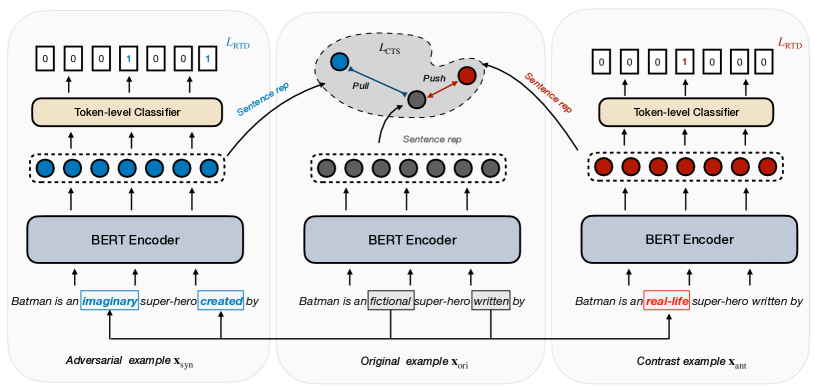
Figure 1: An illustration of our model, note that we use the embedding of [CLS] as the sentence representation.

As stated in the observations in Section 2, we explore strategies that could improve the sensitivity of PLMs. In this section, we present CLINE, a simple and effective method to generate the adversarial and contrastive examples and learn from both of them. We start with the generation of adversarial and contrastive examples in Section 3.1, and then introduce the learning objectives of CLINE in Section 3.2.

3.1 Generation of Examples

We expect that by contrasting sentences with the same and different semantics, our model can be more sensitive to the semantic changes. To do so, we adopt the idea of contrastive learning, which aims to learn the representation by concentrating positive pairs and pushing negative pairs apart. Therefore it is essential to define appropriate positive and negative pairs. In this paper, we regard sentences with the same semantics as positive pairs and sentences with opposite semantics as negative pairs. Some works Alzantot et al. (2018); Tan et al. (2020); Wu et al. (2020) attempt to utilize data augmentation (such as synonym replacement, back translation, etc) to generate positive instances, but few works pay attention to the negative instances. And it is difficult to obtain opposite semantic instances for textual examples.

Intuitively, when we replace the representative words in a sentence with its antonym, the semantic of the sentence is easy to be irrelevant or even opposite to the original sentence. As shown in Figure 1, given the sentence “Batman is an fictional super-hero written by”, we can replace “fictional” with its antonym “real-life”, and then we get a counterfactual sentence “Batman is an real-life super-hero written by”. The latter contradicts the former and forms a negative pair with it.

We generate two sentences from the original input sequence $\bm{x}^{\rm ori}$, which express substantially different semantics but have few different words. One of the sentences is semantically close to $\bm{x}^{\rm ori}$ (denoted as $\bm{x}^{\rm syn}$), while the other is far from or even opposite to $\bm{x}^{\rm ori}$ (denoted as $\bm{x}^{\rm ant}$). In specific, we utilize spaCy to conduct segmentation and POS for the original sentences, extracting verbs, nouns, adjectives, and adverbs. $\bm{x}^{\rm syn}$ is generated by replacing the extracted words with synonyms, hypernyms and morphological changes, and $\bm{x}^{\rm ant}$ is generated by replacing them with antonyms and random words. For $\bm{x}^{\rm syn}$, about 40% tokens are replaced. For $\bm{x}^{\rm ant}$, about 20% tokens are replaced.

3.2 Training Objectives

CLINE trains a neural text encoder (i.e., deep Transformer) $\texttt{E}_{\phi}$ parameterized by $\phi$ that maps a sequence of input tokens $\bm{x}=[x_{1},...,x_{T}]$ to a sequence of representations $\bm{h}=[h_{1},..,h_{T}],h_{i\in[1:T]}\in\mathbb{R}^{d}$, where $d$ is the dimension:

$$\bm{h}=\texttt{E}_{\phi}(\bm{x}).$$ (1)

Masked Language Modeling Objective With random tokens masked by special symbols [MASK], the input sequence is partially corrupted. Following BERT Devlin et al. (2019), we adopt the masked language model objective (denoted as $\mathcal{L}_{\text{MLM}}$), which reconstructs the sequence by predicting the masked tokens.

Replaced Token Detection Objective On the basis of $\bm{x}^{\rm syn}$ and $\bm{x}^{\rm ant}$, we adopt an additional classifier $\mathcal{C}$ for the two generated sequences and detect which tokens are replaced by conducting two-way classification with a sigmoid output layer:

$$p(\bm{x}^{\rm syn},t)=\text{sigmoid}(w^{\top}h^{\rm syn}_{t}),$$ (2)

$$p(\bm{x}^{\rm ant},t)=\text{sigmoid}(w^{\top}h^{\rm ant}_{t}).$$ (3)

The loss, denoted as $\mathcal{L}_{\text{RTD}}$ is computed by:

$$\begin{split}\mathcal{L}_{\text{RTD}}&=\sum_{\bm{x}^{\prime}\in\{x^{\rm syn},x^{\rm ant}\}}-\sum_{t=1}^{T}\delta_{t}\text{log}\ p(\bm{x}^{\prime},t)\\ &-(1-\delta_{t})\text{log}(1-p(\bm{x}^{\prime},t)),\end{split}$$ (4)

where $\delta_{t}=1$ when the token $x_{t}$ is corrupted, and $\delta_{t}=0$ otherwise.

Contrastive Objective The intuition of CLINE is to accurately predict if the semantics are changed when the original sentences are modified. In other words, in feature space, the metric between $\bm{h}^{\rm ori}$ and $\bm{h}^{\rm syn}$ should be close and the metric between $\bm{h}^{\rm ori}$ and $\bm{h}^{\rm ant}$ should be far. Thus, we develop a contrastive objective, where ($\bm{x}^{\rm ori}$, $\bm{x}^{\rm syn}$) is considered a positive pair and ($\bm{x}^{\rm ori}$, $\bm{x}^{\rm ant}$) is negative. We use $h_{c}$ to denote the embedding of the special symbol [CLS]. In the training of CLINE, we follow the setting of RoBERTa Liu et al. (2019) to omit the next sentence prediction (NSP) objective since previous works have shown that NSP objective can hurt the performance on the downstream tasks Liu et al. (2019); Joshi et al. (2020). Alternatively, adopt the embedding of [CLS] as the sentence representation for a contrastive objective. The metric between sentence representations is calculated as the dot product between [CLS] embeddings:

$$f(\bm{x}^{*},\bm{x}^{\prime})=\text{exp}(h_{c}^{*\top}h^{\prime}_{c}).$$ (5)

Inspired by InfoNCE, we define an objective $\mathcal{L}_{\rm cts}$ in the contrastive manner:

$$\mathcal{L}_{\rm cts}\!=\!-\sum_{\bm{x}\in\mathcal{X}}\text{log}\frac{f(\bm{x}^{\rm ori},\bm{x}^{\rm syn})}{f(\bm{x}^{\rm ori},\bm{x}^{\rm syn})+f(\bm{x}^{\rm ori},\bm{x}^{\rm ant})}.$$ (6)

Note that different from some contrastive strategies that usually randomly sample multiple negative examples, we only utilize one $\bm{x}_{\rm ant}$ as the negative example for training. This is because the primary goal of our pre-training objectives is to improve the robustness under semantically adversarial attacking. And we only focus on the negative sample (i.e., $\bm{x}_{\rm ant}$) that is generated for our goal, instead of arbitrarily sampling other sentences from the pre-training corpus as negative samples.

Finally, we have the following training loss:

$$\mathcal{L}\!=\!\lambda_{1}\mathcal{L}_{\text{MLM}}+\lambda_{2}\mathcal{L}_{\text{RTD}}+\lambda_{3}\mathcal{L}_{\rm cts},$$ (7)

where $\lambda_{i}$ is the task weighting learned by training.

4 Experiments

We conduct extensive experiments and analyses to evaluate the effectiveness of CLINE. In this section, we firstly introduce the implementation (Section 4.1) and the datasets (Section 4.2) we used, then we introduce the experiments on contrastive sets (Section 4.3) and adversarial sets (Section 4.4), respectively. Finally, we conduct the ablation study (Section 4.5) and analysis about sentence representation (Section  4.6).

4.1 Implementation

To better acquire the knowledge from the existing pre-trained model, we did not train from scratch but the official RoBERTa-base model. We train for 30K steps with a batch size of 256 sequences of maximum length 512 tokens. We use Adam with a learning rate of 1e-4, $\beta_{1}=0.9$, $\beta_{2}=0.999$, $\epsilon=$1e-8, L2 weight decay of 0.01, learning rate warmup over the first 500 steps, and linear decay of the learning rate. We use 0.1 for dropout on all layers and in attention. The model is pre-trained on 32 NVIDIA Tesla V100 32GB GPUs. Our model is pre-trained on a combination of BookCorpus Zhu et al. (2015) and English Wikipedia datasets, the data BERT used for pre-training.

Model	IMDB			PERSPECTRUM			BoolQ			SNLI
	Ori	Rev	Con	Ori	Rev	Con	Ori	Rev	Con	Ori	Rev	Con
BERT	92.2	89.8	82.4	74.7	72.8	57.6	60.9	57.6	36.1	89.8	73.0	65.1
RoBERTa	93.6	93.0	87.1	80.6	78.8	65.0	69.6	60.6	43.9	90.8	75.2	67.8
CLINE	94.5	93.9	88.5	81.6	80.2	72.2	73.9	63.9	47.8	91.3	76.0	69.2

Table 4: Accuracy on the original test set (Ori) and contrastive test set (Rev). Contrast consistency (Con) is a metric of whether a model makes correct predictions on every element in both the original test set and the contrastive test set.

4.2 Datasets

We evaluate our model on six text classification tasks:

• IMDB Maas et al. (2011) is a sentiment analysis dataset and the task is to predict the sentiment (positive or negative) of a movie review.

• SNLI Bowman et al. (2015) is a natural language inference dataset to judge the relationship between two sentences: whether the second sentence can be derived from entailment, contradiction, or neutral relationship with the first sentence.

• PERSPECTRUM Chen et al. (2019) is a natural language inference dataset to predict whether a relevant perspective is for/against the given claim.

• BoolQ Clark et al. (2019) is a dataset of reading comprehension instances with boolean (yes or no) answers.

• AG Zhang et al. (2015) is a sentence-level classification with regard to four news topics: World, Sports, Business, and Science/Technology.

• MR Pang and Lee (2005) is a sentence-level sentiment classification on positive and negative movie reviews.

4.3 Experiments on Contrastive Sets

We evaluate our model on four contrastive sets: IMDB, PERSPECTRUM, BoolQ and SNLI, which were provided by Contrast Sets Gardner et al. (2020). We compare our approach with BERT and RoBERTa across the original test set (Ori) and contrastive test set (Rev). Contrast consistency (Con) is a metric defined by Gardner et al. (2020) to evaluate whether a model’s predictions are all correct for the same examples in both the original test set and the contrastive test set. We fine-tune each model many times using different learning rates (1e-5,2e-5,3e-5,4e-5,5e-5) and select the best result on the contrastive test set.

From the results shown in Table 4, we can observe that our model outperforms the baseline. Especially in the contrast consistency metric, our method significantly outperforms other methods, which means our model is sensitive to the small change of semantic, rather than simply capturing the characteristics of the dataset. On the other hand, our model also has some improvement on the original test set, which means our method can boost the performance of PLMs on the common examples.

Model	Method	IMDB	AG	MR	SNLI
BERT	Vanilla	88.7	88.8	68.4	48.6
	FreeLB	91.9	93.3	75.9	56.1
RoBERTa	Vanilla	93.9	91.9	79.7	55.1
	FreeLB	95.2	93.5	81.0	58.1
CLINE	Vanilla	94.7	92.3	80.4	55.4
	FreeLB	95.9	94.2	82.1	58.7

Table 5: Accuracy on the adversarial test set.

4.4 Experiments on Adversarial Sets

To evaluate the robustness of the model, we compare our model with BERT and RoBERTa on the vanilla version and FreeLB version across several adversarial test sets. Instead of using an adversarial attacker to attack the model, we use the adversarial examples generated by TextFooler Jin et al. (2020) as a benchmark to evaluate the performance against adversarial examples. TextFooler identifies the important words in the text and then prioritizes to replace them with the most semantically similar and grammatically correct words.

From the experimental results in Table 5, we can observe that our vanilla model achieves higher accuracy on all the four benchmark datasets compared to the vanilla BERT and RoBERTa. By constructing similar semantic adversarial examples and using the contrastive training objective, our model can concentrate the representation of the original example and the adversarial example, and then achieve better robustness. Furthermore, our method is in the pre-training stage, so it can also be combined with the existing adversarial training methods. Compared with the FreeLB version of BERT and RoBERTa, our model can achieve state-of-the-art (SOTA) performances on the adversarial sets. Experimental results on contrastive sets and adversarial sets show that our model is sensitive to semantic changes and keeps robust at the same time.

Dataset	Model	1%			10%			100%
		Ori	Rev	Con	Ori	Rev	Con	Ori	Rev	Con
PERSPECTRUM	CLINE	71.4	60.4	33.6	75.1	69.1	55.3	81.6	80.2	72.2
	w/o RTD	67.3	59.4	29.0	73.4	67.7	53.0	81.1	78.3	68.9
	w/o Hard Negative	59.0	53.0	14.7	71.4	68.8	38.2	80.9	78.2	65.9
	RoBERTa	55.8	54.8	13.8	72.4	66.8	45.2	80.6	78.8	65.0
BoolQ	CLINE	66.7	52.8	33.7	68.1	54.0	36.1	73.9	63.9	47.8
	w/o RTD	64.8	52.5	32.2	68.0	53.7	35.8	72.5	63.0	46.6
	w/o Hard Negative	60.1	49.0	30.0	68.1	53.4	35.2	69.6	61.8	44.5
	RoBERTa	60.9	49.3	27.5	65.2	53.1	32.8	69.6	60.6	43.9

Table 6: Ablation study on the original test set (Ori) and contrastive test set (Rev) of PERSPECTRUM (accuracy) and BoolQ (accuracy). 1% / 10% indicate using 1% / 10% supervised training data respectively. Contrast consistency (Con) is a metric of whether a model makes correct predictions on every element in both the original test set and the contrastive test set.

4.5 Ablation Study

To further analyze the effectiveness of different factors of our CLINE, we choose PERSPECTRUM Chen et al. (2019) and BoolQ Clark et al. (2019) as benchmark datasets and report the ablation test in terms of 1) w/o RTD: we remove the replaced token detection objective ($\mathcal{L}_{\text{RTD}}$) in our model to verify whether our model mainly benefits from the contrastive objective. 2) w/o Hard Negative: we replace the constructed negative examples with random sampling examples to verify whether the negative examples constructed by unsupervised word substitution are better. We also add 1% and 10% settings, meaning using only 1% / 10% data of the training set, to simulate a low-resource scenario and observe how the model performance across different datasets and settings. From Table 6, we can observe that: 1) Our CLINE outperformance RoBERTa on all settings, which indicates that our method is universal and robust. Especially in the low-resource scenario (1% and 10% supervised training data), our method shows a prominent improvement. 2) Compared to the CLINE, w/o RTD just has a little bit of performance degradation. This proves that the improvement of performance mainly benefits from the contrastive objective and the replaced token detection objective can further make the model sensitive to the change of the words. 3) Compared to CLINE, we can see that the w/o Hard Negative has a significant performance degradation in most settings, proving the effectiveness of constructing hard negative instances.

Model	CLS	MEAN	BS
BERT	42.4	45.2	47.0
CLINE-B	58.0	59.2	66.8
RoBERTa	–	42.5	45.1
CLINE-R	42.1	42.8	49.4

Table 7: The max Hits(%) on all layers of the Transformer-based encoder. We compute cosine similarity between sentence representations with the [CLS] token (CLS) and the mean-pooling of the sentence embedding (MEAN). And BS is short for BertScore. CLINE-B means our model trained from the BERT-base model and CLINE-R means our model trained from the RoBERTa-base model.

4.6 Sentence Semantic Representation

To evaluate the semantic sensitivity of the models, we generate 9626 sentence triplets from a sentence-level sentiment analysis dataset MR Pang and Lee (2005). Each of the triples contains an original sentence $x^{ori}$ from MR, a sentence with similar semantics $x^{syn}$ and a sentence with opposite semantic $x^{ant}$. We generate $x^{syn}$/$x^{ant}$ by replacing a word in $x^{ori}$ with its synonym/antonym from WordNet Miller (1995). And then we compute the cosine similarity between sentence pairs with [CLS] token and the mean-pooling of all tokens. And we also use a SOTA algorithm, BertScore Zhang et al. (2020) to compute similarity scores of sentence pairs. We consider cases in which the model correctly identifies the semantic relationship (e.g., if BertScore($x^{ori}$,$x^{syn}$)$>$BertScore($x^{ori}$,$x^{ant}$)) as Hits. And higher Hits means the model can better distinguish the sentences, which express substantially different semantics but have few different words.

We show the max Hits on all layers (from 1 to 12) of Transformers-based encoder in Table 7. We can observe: 1) In the BERT model, using the [CLS] token as sentence representation achieves worse results than mean-pooling, which shows the same conclusion as Sentence-BERT Reimers and Gurevych (2019). And because RoBERTa omits the NSP objective, so its result of CLS has no meaning. 2) The BertScore can compute semantic similarity better than other methods and our method CLINE-B can further improve the Hits. 3) By constructing positive and negative examples for contrastive learning in pre-training stage, our method CLINE-B and CLINE-R learn better sentence representation and detect small semantic changes. 4) We can observe that the RoBERTa has less Hits than BERT, and our CLINE-B has significant improvement compared to BERT. We speculate that there may be two reasons, the first is that BERT can better identify sentence-level semantic changes because it has been trained with the next sentence prediction (NSP) objective in the pre-training stage. And the second is that the BERT is not trained enough, so it can not represent sentence semantics well, and our method can improve the semantic representation ability of the model.

5 Related Work

5.1 Pre-trained Language Models

The PLMs have proven their advantages in capturing implicit language features. Two main research directions of PLMs are autoregressive (AR) pre-training (such as GPT Radford et al. (2018)) and denoising autoencoding (DAE) pre-training (such as BERT Devlin et al. (2019)). AR pre-training aims to predict the next word based on previous tokens but lacks the modeling of the bidirectional context. And DAE pre-training aims to reconstruct the input sequences using left and right context. However, previous works mainly focus on the token-level pre-training tasks and ignore modeling the global semantic of sentences.

5.2 Adversarial Training

To make neural networks more robust to adversarial examples, many defense strategies have been proposed, and adversarial training is widely considered to be the most effective. Different from the image domain, it is more challenging to deal with text data due to its discrete property, which is hard to optimize. Previous works focus on heuristics for creating adversarial examples in the black-box setting. Belinkov and Bisk (2018) manipulate every word in a sentence with synthetic or natural noise in machine translation systems. Iyyer et al. (2018) leverage back-translated to produce paraphrases that have different sentence structures. Recently, Miyato et al. (2017) extend adversarial and virtual adversarial training Miyato et al. (2019) to text classification tasks by applying perturbations to word embeddings rather than discrete input symbols. Following this, many adversarial training methods in the text domain have been proposed and have been applied to the state-of-the-art PLMs. Li and Qiu (2020) introduce a token-level perturbation to improves the robustness of PLMs. Zhu et al. (2020) use the gradients obtained in adversarial training to boost the performance of PLMs. Although many studies seem to achieve a robust representation, our pilot experiments (Section 2) show that there is still a long way to go.

5.3 Contrastive Learning

Contrastive learning is an unsupervised representation learning method, which has been widely used in learning graph representations Velickovic et al. (2019), visual representations van den Oord et al. (2018); He et al. (2020); Chen et al. (2020), response representations Lin et al. (2020b); Su et al. (2020), text representations Iter et al. (2020); Ding et al. (2021) and structured world models Kipf et al. (2020). The main idea is to learn a representation by contrasting positive pairs and negative pairs, which aims to concentrate positive samples and push apart negative samples. In natural language processing (NLP), contrastive self-supervised learning has been widely used for learning better sentence representations. Logeswaran and Lee (2018) sample two contiguous sentences for positive pairs and the sentences from the other document as negative pairs. Luo et al. (2020) present contrastive pretraining for learning denoised sequence representations in a self-supervised manner. Wu et al. (2020) present multiple sentence-level augmentation strategies for contrastive sentence representation learning. The main difference between these works is their various definitions of positive examples. However, recent works pay little attention to the construction of negative examples, only using simple random sampling sentences. In this paper, we propose a negative example construction strategy with opposite semantics to improve the sentence representation learning and the robustness of the pre-trained language model.

6 Conclusion

In this paper, we focus on one specific problem how to train a pre-trained language model with robustness against adversarial attacks and sensitivity to small changed semantics. We propose CLINE, a simple and effective method to tackle the challenge. In the training phase of CLINE, it automatically generates the adversarial example and semantic negative example to the original sentence. And then the model is trained by three objectives to make full utilization of both sides of examples. Empirical results demonstrate that our method could considerably improve the sensitivity of pre-trained language models and meanwhile gain robustness.

References

- Alzantot et al. (2018) Moustafa Alzantot, Yash Sharma, Ahmed Elgohary, Bo-Jhang Ho, Mani B. Srivastava, and Kai-Wei Chang. 2018. Generating natural language adversarial examples. In Proceedings of the 2018 Conference on Empirical Methods in Natural Language Processing, Brussels, Belgium, October 31 - November 4, 2018, pages 2890–2896. Association for Computational Linguistics.
- Belinkov and Bisk (2018) Yonatan Belinkov and Yonatan Bisk. 2018. Synthetic and natural noise both break neural machine translation. In 6th International Conference on Learning Representations, ICLR 2018, Vancouver, BC, Canada, April 30 - May 3, 2018, Conference Track Proceedings. OpenReview.net.
- Bowman et al. (2015) Samuel R. Bowman, Gabor Angeli, Christopher Potts, and Christopher D. Manning. 2015. A large annotated corpus for learning natural language inference. In Proceedings of the 2015 Conference on Empirical Methods in Natural Language Processing, EMNLP 2015, Lisbon, Portugal, September 17-21, 2015, pages 632–642. The Association for Computational Linguistics.
- Chen et al. (2019) Sihao Chen, Daniel Khashabi, Wenpeng Yin, Chris Callison-Burch, and Dan Roth. 2019. Seeing things from a different angle: Discovering diverse perspectives about claims. In Proceedings of the 2019 Conference of the North American Chapter of the Association for Computational Linguistics: Human Language Technologies, NAACL-HLT 2019, Minneapolis, MN, USA, June 2-7, 2019, Volume 1 (Long and Short Papers), pages 542–557. Association for Computational Linguistics.
- Chen et al. (2020) Ting Chen, Simon Kornblith, Mohammad Norouzi, and Geoffrey E. Hinton. 2020. A simple framework for contrastive learning of visual representations. In Proceedings of the 37th International Conference on Machine Learning, ICML 2020, 13-18 July 2020, Virtual Event, volume 119 of Proceedings of Machine Learning Research, pages 1597–1607. PMLR.
- Clark et al. (2019) Christopher Clark, Kenton Lee, Ming-Wei Chang, Tom Kwiatkowski, Michael Collins, and Kristina Toutanova. 2019. Boolq: Exploring the surprising difficulty of natural yes/no questions. In Proceedings of the 2019 Conference of the North American Chapter of the Association for Computational Linguistics: Human Language Technologies, NAACL-HLT 2019, Minneapolis, MN, USA, June 2-7, 2019, Volume 1 (Long and Short Papers), pages 2924–2936. Association for Computational Linguistics.
- Devlin et al. (2019) Jacob Devlin, Ming-Wei Chang, Kenton Lee, and Kristina Toutanova. 2019. BERT: pre-training of deep bidirectional transformers for language understanding. In Proceedings of the 2019 Conference of the North American Chapter of the Association for Computational Linguistics: Human Language Technologies, NAACL-HLT 2019, Minneapolis, MN, USA, June 2-7, 2019, Volume 1 (Long and Short Papers), pages 4171–4186. Association for Computational Linguistics.
- Ding et al. (2021) Ning Ding, Xiaobin Wang, Yao Fu, Guangwei Xu, Rui Wang, Pengjun Xie, Ying Shen, Fei Huang, Hai-Tao Zheng, and Rui Zhang. 2021. Prototypical representation learning for relation extraction. In International Conference on Learning Representations.
- Gao et al. (2021) Tianyu Gao, Xingcheng Yao, and Danqi Chen. 2021. Simcse: Simple contrastive learning of sentence embeddings. CoRR, abs/2104.08821.
- Gardner et al. (2020) Matt Gardner, Yoav Artzi, Victoria Basmova, Jonathan Berant, Ben Bogin, Sihao Chen, Pradeep Dasigi, Dheeru Dua, Yanai Elazar, Ananth Gottumukkala, Nitish Gupta, Hannaneh Hajishirzi, Gabriel Ilharco, Daniel Khashabi, Kevin Lin, Jiangming Liu, Nelson F. Liu, Phoebe Mulcaire, Qiang Ning, Sameer Singh, Noah A. Smith, Sanjay Subramanian, Reut Tsarfaty, Eric Wallace, Ally Zhang, and Ben Zhou. 2020. Evaluating models’ local decision boundaries via contrast sets. In Proceedings of the 2020 Conference on Empirical Methods in Natural Language Processing: Findings, EMNLP 2020, Online Event, 16-20 November 2020, pages 1307–1323. Association for Computational Linguistics.
- Garg and Ramakrishnan (2020) Siddhant Garg and Goutham Ramakrishnan. 2020. BAE: bert-based adversarial examples for text classification. In Proceedings of the 2020 Conference on Empirical Methods in Natural Language Processing, EMNLP 2020, Online, November 16-20, 2020, pages 6174–6181. Association for Computational Linguistics.
- He et al. (2020) Kaiming He, Haoqi Fan, Yuxin Wu, Saining Xie, and Ross B. Girshick. 2020. Momentum contrast for unsupervised visual representation learning. In 2020 IEEE/CVF Conference on Computer Vision and Pattern Recognition, CVPR 2020, Seattle, WA, USA, June 13-19, 2020, pages 9726–9735. IEEE.
- Iter et al. (2020) Dan Iter, Kelvin Guu, Larry Lansing, and Dan Jurafsky. 2020. Pretraining with contrastive sentence objectives improves discourse performance of language models. In Proceedings of the 58th Annual Meeting of the Association for Computational Linguistics, ACL 2020, Online, July 5-10, 2020, pages 4859–4870. Association for Computational Linguistics.
- Iyyer et al. (2018) Mohit Iyyer, John Wieting, Kevin Gimpel, and Luke Zettlemoyer. 2018. Adversarial example generation with syntactically controlled paraphrase networks. In Proceedings of the 2018 Conference of the North American Chapter of the Association for Computational Linguistics: Human Language Technologies, NAACL-HLT 2018, New Orleans, Louisiana, USA, June 1-6, 2018, Volume 1 (Long Papers), pages 1875–1885. Association for Computational Linguistics.
- Jiang et al. (2020) Haoming Jiang, Pengcheng He, Weizhu Chen, Xiaodong Liu, Jianfeng Gao, and Tuo Zhao. 2020. SMART: robust and efficient fine-tuning for pre-trained natural language models through principled regularized optimization. In Proceedings of the 58th Annual Meeting of the Association for Computational Linguistics, ACL 2020, Online, July 5-10, 2020, pages 2177–2190. Association for Computational Linguistics.
- Jin et al. (2020) Di Jin, Zhijing Jin, Joey Tianyi Zhou, and Peter Szolovits. 2020. Is BERT really robust? A strong baseline for natural language attack on text classification and entailment. In The Thirty-Fourth AAAI Conference on Artificial Intelligence, AAAI 2020, New York, NY, USA, February 7-12, 2020, pages 8018–8025. AAAI Press.
- Joshi et al. (2020) Mandar Joshi, Danqi Chen, Yinhan Liu, Daniel S. Weld, Luke Zettlemoyer, and Omer Levy. 2020. Spanbert: Improving pre-training by representing and predicting spans. Trans. Assoc. Comput. Linguistics, 8:64–77.
- Kaushik et al. (2020) Divyansh Kaushik, Eduard H. Hovy, and Zachary Chase Lipton. 2020. Learning the difference that makes A difference with counterfactually-augmented data. In 8th International Conference on Learning Representations, ICLR 2020, Addis Ababa, Ethiopia, April 26-30, 2020. OpenReview.net.
- Kipf et al. (2020) Thomas N. Kipf, Elise van der Pol, and Max Welling. 2020. Contrastive learning of structured world models. In 8th International Conference on Learning Representations, ICLR 2020, Addis Ababa, Ethiopia, April 26-30, 2020. OpenReview.net.
- Li et al. (2020) Linyang Li, Ruotian Ma, Qipeng Guo, Xiangyang Xue, and Xipeng Qiu. 2020. BERT-ATTACK: adversarial attack against BERT using BERT. In Proceedings of the 2020 Conference on Empirical Methods in Natural Language Processing, EMNLP 2020, Online, November 16-20, 2020, pages 6193–6202. Association for Computational Linguistics.
- Li and Qiu (2020) Linyang Li and Xipeng Qiu. 2020. Textat: Adversarial training for natural language understanding with token-level perturbation. CoRR, abs/2004.14543.
- Lin et al. (2020a) Gongqi Lin, Yuan Miao, Xiaoyong Yang, Wenwu Ou, Lizhen Cui, Wei Guo, and Chunyan Miao. 2020a. Commonsense knowledge adversarial dataset that challenges ELECTRA. In 16th International Conference on Control, Automation, Robotics and Vision, ICARCV 2020, Shenzhen, China, December 13-15, 2020, pages 315–320. IEEE.
- Lin et al. (2020b) Zibo Lin, Deng Cai, Yan Wang, Xiaojiang Liu, Haitao Zheng, and Shuming Shi. 2020b. The world is not binary: Learning to rank with grayscale data for dialogue response selection. In Proceedings of the 2020 Conference on Empirical Methods in Natural Language Processing, EMNLP 2020, Online, November 16-20, 2020, pages 9220–9229. Association for Computational Linguistics.
- Liu et al. (2019) Yinhan Liu, Myle Ott, Naman Goyal, Jingfei Du, Mandar Joshi, Danqi Chen, Omer Levy, Mike Lewis, Luke Zettlemoyer, and Veselin Stoyanov. 2019. Roberta: A robustly optimized BERT pretraining approach. CoRR, abs/1907.11692.
- Logeswaran and Lee (2018) Lajanugen Logeswaran and Honglak Lee. 2018. An efficient framework for learning sentence representations. In 6th International Conference on Learning Representations, ICLR 2018, Vancouver, BC, Canada, April 30 - May 3, 2018, Conference Track Proceedings. OpenReview.net.
- Luo et al. (2020) Fuli Luo, Pengcheng Yang, Shicheng Li, Xuancheng Ren, and Xu Sun. 2020. CAPT: contrastive pre-training for learning denoised sequence representations. CoRR, abs/2010.06351.
- Maas et al. (2011) Andrew L. Maas, Raymond E. Daly, Peter T. Pham, Dan Huang, Andrew Y. Ng, and Christopher Potts. 2011. Learning word vectors for sentiment analysis. In The 49th Annual Meeting of the Association for Computational Linguistics: Human Language Technologies, Proceedings of the Conference, 19-24 June, 2011, Portland, Oregon, USA, pages 142–150. The Association for Computer Linguistics.
- Michel et al. (2019) Paul Michel, Xian Li, Graham Neubig, and Juan Miguel Pino. 2019. On evaluation of adversarial perturbations for sequence-to-sequence models. In Proceedings of the 2019 Conference of the North American Chapter of the Association for Computational Linguistics: Human Language Technologies, NAACL-HLT 2019, Minneapolis, MN, USA, June 2-7, 2019, Volume 1 (Long and Short Papers), pages 3103–3114. Association for Computational Linguistics.
- Miller (1995) George A. Miller. 1995. Wordnet: A lexical database for english. Commun. ACM, 38(11):39–41.
- Miyato et al. (2017) Takeru Miyato, Andrew M. Dai, and Ian J. Goodfellow. 2017. Adversarial training methods for semi-supervised text classification. In 5th International Conference on Learning Representations, ICLR 2017, Toulon, France, April 24-26, 2017, Conference Track Proceedings. OpenReview.net.
- Miyato et al. (2019) Takeru Miyato, Shin-ichi Maeda, Masanori Koyama, and Shin Ishii. 2019. Virtual adversarial training: A regularization method for supervised and semi-supervised learning. IEEE Trans. Pattern Anal. Mach. Intell., 41(8):1979–1993.
- van den Oord et al. (2018) Aäron van den Oord, Yazhe Li, and Oriol Vinyals. 2018. Representation learning with contrastive predictive coding. CoRR, abs/1807.03748.
- Pang and Lee (2005) Bo Pang and Lillian Lee. 2005. Seeing stars: Exploiting class relationships for sentiment categorization with respect to rating scales. In ACL 2005, 43rd Annual Meeting of the Association for Computational Linguistics, Proceedings of the Conference, 25-30 June 2005, University of Michigan, USA, pages 115–124. The Association for Computer Linguistics.
- Radford et al. (2018) Alec Radford, Karthik Narasimhan, Tim Salimans, and Ilya Sutskever. 2018. Improving language understanding by generative pre-training.
- Reimers and Gurevych (2019) Nils Reimers and Iryna Gurevych. 2019. Sentence-bert: Sentence embeddings using siamese bert-networks. In Proceedings of the 2019 Conference on Empirical Methods in Natural Language Processing and the 9th International Joint Conference on Natural Language Processing, EMNLP-IJCNLP 2019, Hong Kong, China, November 3-7, 2019, pages 3980–3990. Association for Computational Linguistics.
- Su et al. (2020) Yixuan Su, Deng Cai, Qingyu Zhou, Zibo Lin, Simon Baker, Yunbo Cao, Shuming Shi, Nigel Collier, and Yan Wang. 2020. Dialogue response selection with hierarchical curriculum learning. CoRR, abs/2012.14756.
- Tan et al. (2020) Samson Tan, Shafiq R. Joty, Min-Yen Kan, and Richard Socher. 2020. It’s morphin’ time! combating linguistic discrimination with inflectional perturbations. In Proceedings of the 58th Annual Meeting of the Association for Computational Linguistics, ACL 2020, Online, July 5-10, 2020, pages 2920–2935. Association for Computational Linguistics.
- Velickovic et al. (2019) Petar Velickovic, William Fedus, William L. Hamilton, Pietro Liò, Yoshua Bengio, and R. Devon Hjelm. 2019. Deep graph infomax. In 7th International Conference on Learning Representations, ICLR 2019, New Orleans, LA, USA, May 6-9, 2019. OpenReview.net.
- Wang and Bansal (2018) Yicheng Wang and Mohit Bansal. 2018. Robust machine comprehension models via adversarial training. In Proceedings of the 2018 Conference of the North American Chapter of the Association for Computational Linguistics: Human Language Technologies, NAACL-HLT, New Orleans, Louisiana, USA, June 1-6, 2018, Volume 2 (Short Papers), pages 575–581. Association for Computational Linguistics.
- Wu et al. (2020) Zhuofeng Wu, Sinong Wang, Jiatao Gu, Madian Khabsa, Fei Sun, and Hao Ma. 2020. CLEAR: contrastive learning for sentence representation. CoRR, abs/2012.15466.
- Zang et al. (2020) Yuan Zang, Fanchao Qi, Chenghao Yang, Zhiyuan Liu, Meng Zhang, Qun Liu, and Maosong Sun. 2020. Word-level textual adversarial attacking as combinatorial optimization. In Proceedings of the 58th Annual Meeting of the Association for Computational Linguistics, ACL 2020, Online, July 5-10, 2020, pages 6066–6080. Association for Computational Linguistics.
- Zhang et al. (2020) Tianyi Zhang, Varsha Kishore, Felix Wu, Kilian Q. Weinberger, and Yoav Artzi. 2020. Bertscore: Evaluating text generation with BERT. In 8th International Conference on Learning Representations, ICLR 2020, Addis Ababa, Ethiopia, April 26-30, 2020. OpenReview.net.
- Zhang et al. (2015) Xiang Zhang, Junbo Jake Zhao, and Yann LeCun. 2015. Character-level convolutional networks for text classification. In Advances in Neural Information Processing Systems 28: Annual Conference on Neural Information Processing Systems 2015, December 7-12, 2015, Montreal, Quebec, Canada, pages 649–657.
- Zhu et al. (2020) Chen Zhu, Yu Cheng, Zhe Gan, Siqi Sun, Tom Goldstein, and Jingjing Liu. 2020. Freelb: Enhanced adversarial training for natural language understanding. In 8th International Conference on Learning Representations, ICLR 2020, Addis Ababa, Ethiopia, April 26-30, 2020. OpenReview.net.
- Zhu et al. (2015) Yukun Zhu, Ryan Kiros, Richard S. Zemel, Ruslan Salakhutdinov, Raquel Urtasun, Antonio Torralba, and Sanja Fidler. 2015. Aligning books and movies: Towards story-like visual explanations by watching movies and reading books. In 2015 IEEE International Conference on Computer Vision, ICCV 2015, Santiago, Chile, December 7-13, 2015, pages 19–27. IEEE Computer Society.