What do End-to-End Speech Models Learn about Speaker, Language and Channel Information?
A Layer-wise and Neuron-level Analysis

Abstract

Deep neural networks are inherently opaque and challenging to interpret. Unlike hand-crafted feature-based models, we struggle to comprehend the concepts learned and how they interact within these models. This understanding is crucial not only for debugging purposes but also for ensuring fairness in ethical decision-making. In our study, we conduct a post-hoc functional interpretability analysis of pretrained speech models using the probing framework [1]. Specifically, we analyze utterance-level representations of speech models trained for various tasks such as speaker recognition and dialect identification. We conduct layer and neuron-wise analyses, probing for speaker, language, and channel properties. Our study aims to answer the following questions: i) what information is captured within the representations? ii) how is it represented and distributed? and iii) can we identify a minimal subset of the network that possesses this information? Our results reveal several novel findings, including: i) channel and gender information are distributed across the network, ii) the information is redundantly available in neurons with respect to a task, iii) complex properties such as dialectal information are encoded only in the task-oriented pretrained network, iv) and is localised in the upper layers, v) we can extract a minimal subset of neurons encoding the pre-defined property, vi) salient neurons are sometimes shared between properties, vii) our analysis highlights the presence of biases (for example gender) in the network. Our cross-architectural comparison indicates that: i) the pretrained models capture speaker-invariant information, and ii) CNN models are competitive with Transformer models in encoding various understudied properties.

1 Introduction

Deep Neural Networks (DNNs) have constantly pushed the state-of-the-art in all arenas of Artificial Intelligence including Natural Language Processing (NLP) [2] and Computer Vision (CV) [3]. Impressive strides have also been made in speech technologies, for example, Automatic Speech Recognition (ASR) [4, 5, 6, 7, 8, 9], Pretrained Speech Transformers [10, 11, 12, 13], Dialect, Language and Speaker Identification [14, 15, 16, 17, 18, 19, 20] models. While deep neural networks provide a simple and elegant end-to-end framework with a flexible training mechanism, the output models are inherently black-box. In contrast to traditional models, they lack an explanation of what knowledge is captured within the learned representations, and how it is used by the model during prediction. The opaqueness of deep neural models hinders practitioners from understanding their internal mechanics, which is crucial not only for debugging but also for ethical decision-making and fairness in these systems [21, 22]. These internal mechanics include metrics that are often as important as the models’ performance. As a result, a plethora of research has been conducted to investigate how deep neural models encode auxiliary knowledge in their learned representations through classifiers [23, 24, 25, 26], visualizations [27, 28], ablation studies [29, 30], and unsupervised methods [31, 32, 33].

In this paper, we focus our efforts on studying pretrained speech models. It is challenging to understand and interpret the outputs of speech models, mainly due to the variable lengths of the input signals and the complex hierarchical structures that exist at different time scales. Furthermore, environmental factors such as channel information (e.g., signal recording and transmission quality of speech) and speaker information (voice identity, gender, age, and language) can influence the characteristics of the input signal; and make it more challenging to comprehend the models’ decisions. Speaker recognition (SR) systems, for instance, involve the processing of personal data, and are highly susceptible to biases [34]. Therefore, it is essential to study and interpret other factors that could influence the model’s decision, such as gender, race, accent, and the characteristics of the microphone used. While some prior research has focused on interpreting the representations in speech models [35, 36, 37, 38, 39, 40], no fine-grained neuron-level analysis has been carried out.

A prominent framework for probing in the NLP domain is the Probing Classifiers [25], which has been extensively used to analyze representations at the level of individual layers [36, 37, 38, 39], attention heads [41], and a more fine-grained neuron level [23, 42, 43]. These studies reveal interesting findings, such as how different linguistic properties, such as morphology and syntax, are captured in different parts of the network, and how certain properties are more localized or distributed than others. Furthermore, the Probing Classifiers framework has been applied to the analysis of individual neurons, enabling a more comprehensive understanding of the network [44, 45, 46, 23, 42, 43, 47]. It also holds significant potential for various applications, including system manipulation [30] and model distillation [48, 49].

We use probing classifiers to conduct a post-hoc functional interpretation. Our analysis includes a layer-wise and fine-grained neuron-level examination of the pretrained speech models, specifically focusing on: i) speaker information such as gender and voice identity, ii) language and its dialectal variants, and iii) channel information, using utterance-level representation. Our study is guided by the following research questions: i) does the end-to-end speech model capture different properties (e.g. gender, channel, or speaker information)? ii) where in the network is it represented, and how localized or distributed is it?

We follow a simple methodology: i) extract the representations (of speech utterances) from our studied pretrained model; ii) train an auxiliary classifier towards predicting the studied properties; iii) the accuracy of the classifier serves as a proxy to the quality of the learned representation with respect to that property. We train classifiers using different layers to carry out our layer-wise analysis and do a fine-grained analysis by probing for neurons that capture these properties.

We investigate four pretrained end-to-end architectures: two Convolutional Neural Networks (CNN) architectures trained for the tasks of i) speaker recognition and ii) dialect identification, as well as two Transformer architectures trained to iii) reconstruct the masked signal. We chose these architectures because they have demonstrated state-of-the-art performance in various speech tasks. Additionally, comparing CNNs to the recently emerged Transformer architecture provides interesting cross-architectural analysis. Our probes are trained to capture the following extrinsic properties of interest: i) gender classification, ii) speaker verification, iii) language identification, iv) dialect, and v) channel classification. Our cross-architectural analysis shows that:

• Minimal Neuron Subset: Simple properties, such as gender, can be encoded with minimal neuron activation (approximately 1-5%). Complex properties such as regional dialect identification or voice identification requires a larger subset of neurons to achieve optimal accuracy.

• Task-specific Redundancy: Gender and channel information are redundantly observed in both layer and neuron analyses. These phenomena are distributed across the network and can be captured redundantly with a small number of neurons from any part of the network. Similar redundancy is also observed in encoding language properties.

• Localized vs Distributive: The salient neurons are localized in the final layers of the pretrained models, indicating that the deeper layers of the network are more informative and capture more abstract information. This observation was true for both simple and complex tasks.

• Robustness: Most of the understudied pretrained models learn speaker-invariant information.

• Polysemous Neurons: Neurons are multivariate in nature and shared among properties. For example, some neurons were found to be salient for both voice identity and gender properties.

• Bias: We were able to highlight neurons responsible for sensitive information (e.g., gender). This can be potentially useful to mitigate representation bias in the models.

• Pretrained Models for Transfer learning: Pretrained convolutional neural networks (CNNs) can provide comparable, or even superior, performance compared to speech transformers. These CNNs are commonly used as feature extractors or for fine-tuning in downstream tasks. In line with the findings of [52], our results highlight the potential of utilizing large pretrained CNNs as effective alternatives to pretrained speech transformers.

To the best of our knowledge, our study represents the first attempt at conducting a large-scale analysis of neurons. While other contemporary works, such as [53, 37, 39, 54, 35, 38, 55] have largely focused on layer-wise analysis, our work goes beyond and delves into a more fine-grained, neuron-level analysis. This microscopic view of speech representation opens up potential applications, including neuron manipulation and network pruning, among others, which can greatly benefit from our findings.

2 Related Work

The rise of deep Neural Networks has seen a subsequent rise in interpretability studies, due to the black-box nature of these models. One of the commonly used interpretation technique is the probing-tasks or the diagnostic-classifiers framework [25]. This approach has been used to probe for different linguistic properties captured within the network. For example researchers probed for: i) morphology using attention weights [41], or recurrent neural network (RNN)/transformer representations [56, 57, 58], in neural machine translation (NMT) [25, 26] and language models (LM) neurons [23, 59], ii) anaphora [60], iii) lexical semantics with LM and NMT states [25, 26], and iv) word presence [61], subject-verb-agreement [62], relative islands [63], number agreement [64], semantic roles [65], syntactic information [57, 62, 66, 63, 67] among others using hidden states. Detailed comprehensive surveys are presented in [68, 69].

In the arena of speech modeling, a handful of properties have been examined, namely: i) utterance length, word presence, and homonym disambiguation using audio-visual RNN states [70]; ii) phonemes and other phonetic features using CNN activation in end-to-end speech recognition, [71, 72, 73] using activations in the feed-forward network of the acoustic model, [74] using RNNs; along with iii) formants and other prosodic features examined in the CNNs trained from raw speech [35]; iv) gender [71, 39, 37]; v) speaker information [39, 37], style, and accent [36] using network activations; vi) channel [39, 37] using activations; vii) fluency, pronunciation, and other audio features from transformers [38]; viii) word properties, phonetic information using several self-supervised model layers [55]; ix) frame classification, segment classification, fundamental frequency tracking, and duration prediction using the autoregressive predictive coding (APC) approach [54]; and x) linguistic information from emotion recognition transformer models [75]. Apart from classification, other methods for finding associations include:

• Computing correlations or similarities: e.g. with other acoustic features [76], or similarity between representations learned by different models [53]

• Regression: e.g. sentence length with encoder neurons in NeuralMT [47]

• Clustering: e.g. word class using A/V CNN embeddings [31]

• Detecting change point of activation: e.g. using RNN gates for finding phoneme boundaries [77]

• Visualisation: e.g. in deep CNN models by sampling image patches [44, 78, 79] or by generating images [45] that maximize the activation of each individual neuron among others

Building upon the research conducted in [23, 37], our approach leverages proxy classifiers to gain valuable insights into the encoded information within pretrained deep learning networks. However, our approach differs from theirs in that we have analyzed various types of pretrained models, incorporating different objective functions and architectures. In addition to analyzing the dialectal model, ADI, as utilized in [37], we have further explored a speaker recognition model with a similar architecture. Furthermore, our research represents the pioneering effort in exploring pretrained speech models through fine-grained neuron-level analysis.

Diverging from the approaches taken in [39, 37], our study focuses on analyzing individual or groups of neurons that effectively encode specific properties. Taking inspiration from [23], which probed neurons learning linguistic properties in deep language models, our research represents the first attempt to closely examine the neurons within pretrained speech networks that capture speaker, language, and channel properties.

3 Methodology

Our methodology is based on the probing framework called the Diagnostic Classifiers. We extract activations from the pretrained neural network model $\mathds{M}$ and use these as static features to train a classifier $\mathds{P}$ towards the task of predicting a certain property. The underlying assumption is that if the classifier $\mathds{P}$ successfully predicts the property, the representations implicitly encode this information. We extract the representations from the individual layers for our layer-wise analysis (Section 3.1) and the entire network for the neuron-analysis (Section 3.2).

Neuron Analysis

We use the LCA method [23] to generate a neuron ranking with respect to the property of interest. The classifier is trained by minimizing the following loss function:

$$\mathcal{L}(\theta)=-\sum_{i}\log P_{\theta}(t_{u_{i}}|u_{i})$$

where $P_{\theta}(t_{u_{i}}|u_{i})=\frac{\exp(\theta_{l}\cdot z_{i})}{\sum_{l^{\prime}}\exp(\theta_{l^{\prime}}\cdot z_{i})}$ is the probability that utterance $u_{i}$ is classified as property $t_{u_{i}}$. The weights $\theta\in\mathds{R}^{D\times|T|}$ are learned with gradient descent. Here $D$ is the dimensionality of the vector representations $z_{i}$ (of the utterance $u_{i}$) and $|T|$ is the number of properties the classifier is predicting. Given the trained weights, $\theta$ ($\theta\in\mathds{R}^{D\times|T|}$), of the classifier $\mathds{P}$, we want to extract a ranking of the $D$ neurons in the model $\mathds{M}$. For the property $t\in T$, we sort the weights $\theta_{t}\in\mathds{R}^{D}$ by their absolute values in descending order. Hence, the neuron with the highest corresponding absolute weight in $\theta_{t}$ appears at the top of our ranking. We consider the top $n$ neurons (for the individual property under consideration) that cumulatively contribute to some percentage of the total weight mass as salient neurons. The complete process is illustrated in Figure 1.

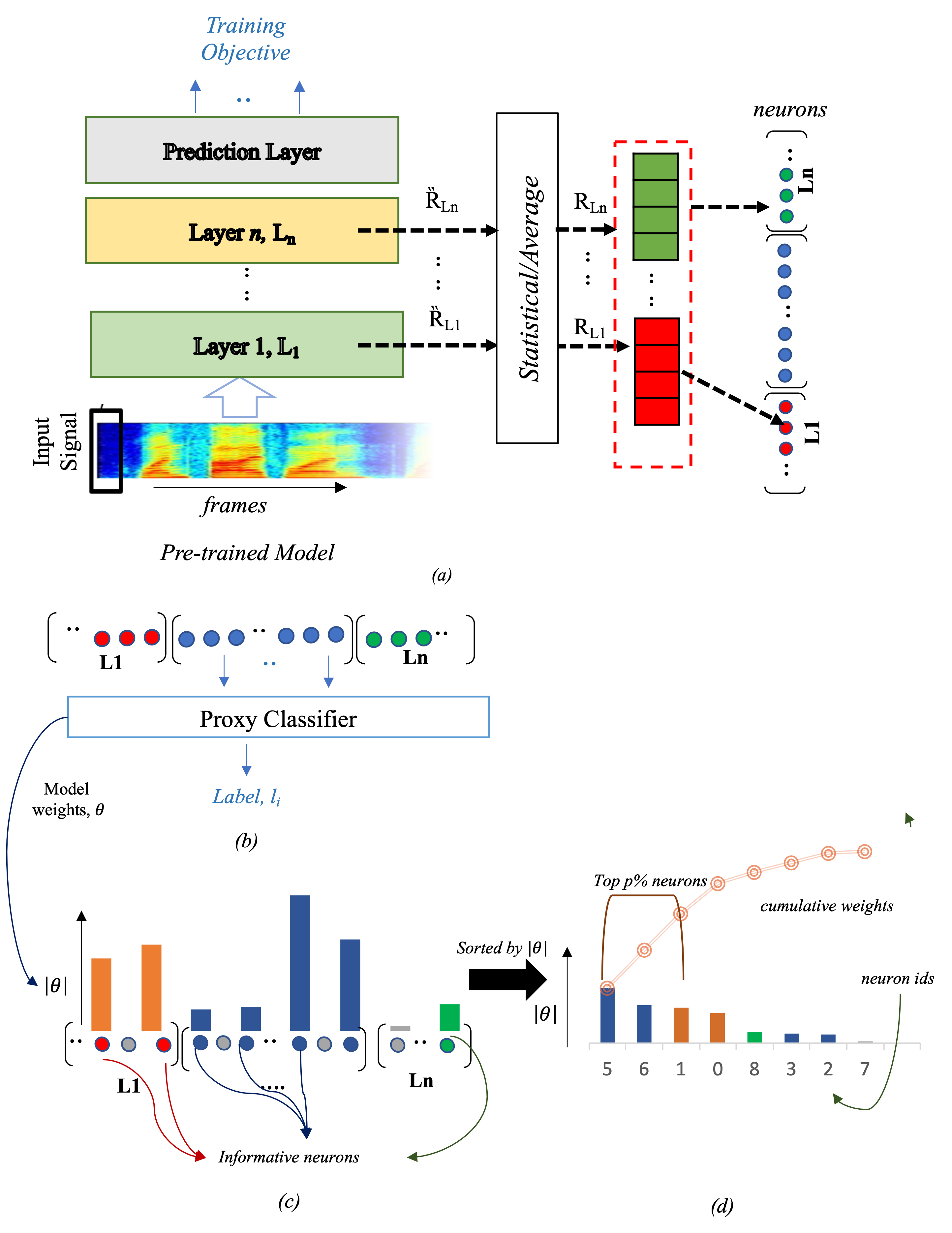
Figure 1: Experimental pipeline of the study: In Figure 1(a), the process of converting frame-level representation, denoted as $\ddot{\mathcal{R}}_{l}$, to utterance-level representation, denoted as $\mathcal{R}_{l}$, using average/statistical polling is depicted. Figure 1(b) illustrates the proxy classifier, Figures 1(c) and 1(d) demonstrate the utilization of trained weights from the proxy classifier for ranking the neurons in the pipeline.

The methodology employed in this study serves two overarching objectives: first, to analyze speech models in order to gain insights into the specific properties encoded within the networks, and second, to assess the degree of localization or distribution of these properties across different layers of the network. In particular, we investigate the presence of three key properties: i) speaker information, such as gender and voice identity; ii) language information, including language and dialect identification; iii) and transmission channel information.

3.1 Utterance-level Representation

For a given temporal ordered feature sequence input, with $F$ number of frames and $D$ feature dimension ($D\times F$), we first extract the latent frame ($\ddot{\mathcal{R}}_{l}$) or utterance-level ($\mathcal{R}_{l}$) speech representation from the layers ($l$) of the pretrained neural network model $\mathds{M}$. Since our goal is to study utterance level representation $\mathcal{R}_{l}$ for a layer $l$, we aggregate the frame-level representations by passing it through a statistical/average pooling function ($\varphi^{[l]}$), $\mathcal{R}_{l}=\varphi^{[l]}(\ddot{\mathcal{R}}_{l})$. For the entire network representation, we concatenate the layers ($l$) to obtain $ALL=\mathcal{R}{l_{1}}+\mathcal{R}{l_{2}}+\ldots+\mathcal{R}_{l_{L}}$, where $L$ represents the total number of layers.

3.2 Proxy Classifier

Given a dataset of $N$ utterances $\mathbb{U}=\{u_{1},u_{2},...,u_{N}\}$ with a corresponding set of annotation classes $C=\{c_{1},c_{2},...,c_{C}\}$, we map each utterance $u_{i}$, in the data to the latent utterance-level representations using pretrained model $\mathds{M}$. We use a simple logistic regression model ($\mathds{P}$) trained by minimising the cross entropy loss $H$. The accuracy of the trained classifier serves as a proxy to indicate that the model representations have learned the underlying property.

Neuron Analysis

We use the weights of the trained classifier to measure the importance of neurons with respect to the understudied property. Because neurons are multi-variate in nature, we additionally use elastic-net regularization [80]:

$$\mathcal{L}(\theta)=H_{\theta}+\lambda_{1}\left\|\theta\right\|_{1}+\lambda_{2}\left\|\theta\right\|_{2}^{2}$$ (1)

where $\theta$ represents the learned weights in the classifier and $\lambda_{1}\left\|\theta\right\|_{1}$ and $\lambda_{2}\left\|\theta\right\|_{2}^{2}$ correspond to $L_{1}$ and $L_{2}$ regularization respectively. The combination of $L_{1}$ and $L_{2}$ regularization creates a balance between selecting very focused localised features ($L_{1}$) vs distributed neurons ($L_{2}$) shared among many properties.

Function TopNeurons($\theta,p$):

       $\theta_{top,c}\longleftarrow[][]$ $\triangleright$ To store top neurons per class-label

      foreach $class,c\in C$ do

             $tm\longleftarrow\sum_{n=1}^{N}|\theta_{n}^{c}|$ $\triangleright$ total mass

            $\theta_{s}\longleftarrow sort(\theta^{c})$ $\triangleright$ sorted list by weight

            $\theta_{cm}\longleftarrow cumulativeSum(\theta_{s})$

            $\theta_{top,c}\longleftarrow\theta_{cm}<p*tm$ $\triangleright$ top neurons per class with threshold p

       end foreach

      $\theta_{top}\longleftarrow\bigcup_{c=1}^{C}\theta_{top,c}$ $\triangleright$ top neurons for all the classes

      return $\theta_{top}$

Algorithm 1 Top Neuron Ranking

3.3 Selecting Salient Neurons

Our goal is to determine the relative importance of intermediate neurons in relation to specific task properties. To achieve this, we rank the neurons based on their significance for each class label $c$. Using the trained proxy classifier $\mathds{P}$, we first arrange the absolute weight values of the neurons $|\theta_{n}^{c}|$ in descending order, and then calculate the cumulative weight vector (as illustrated in Figure 1c-d). The total mass is defined by the sum of the weight vector, and each element $n$ indicates the portion of the weight mass covered by the first $n$ neurons. Subsequently, we select the top p% of neurons, corresponding to the cumulative weights that constitute a certain percentage of the total mass. To find the salient neurons for each class, we initialize with a small percentage ($p=0.1\%$) of the total mass. Then, the percentage is iteratively increased, while adding the newly discovered important neurons ($salient\_neurons$ $\leftarrow$ TopNeurons($\theta$,p) $\setminus$ $salient\_neurons$) to the list ordered by importance towards the task [59]. The algorithm terminates when the salient neurons achieve accuracy close to the Oracle (i.e., accuracy using the entire network) within a predefined threshold. Further details can be found in Section 3.3.2. Finally, we combine all the selected class-wise neurons to determine the overall top neurons of the network (see Algorithm 1 for specifics).

3.3.1 Efficacy of the Ranking

We evaluate the effectiveness of neuron ranking for encoded information using ablation. More specifically, we select the top/bottom/random 20% of neurons, while masking-out, the remaining from the ranked list as prescribed in [23]. Next, we re-evaluated the test set using the previously trained proxy classifier.

3.3.2 Minimal Neuron Set

To obtain a minimal neuron set for the proxy task, we iteratively gather an array of top $N$% of neurons and re-train the proxy classifier with the selected neurons only. We repeat this method until we converge to Oracle performance (Accuracy) i.e. with the model trained with all the neurons (‘ALL’) of the network. We use a threshold of $\delta=1.0$ as our convergence criteria i.e. the number of neurons sufficiently capture a property if retraining classifier, using them, results in only $1\%$ loss in accuracy. We select the neuron set with the highest accuracy close to $[Acc(ALL)\pm\delta]$.

3.4 Control tasks

Using probing classifiers for analysis presents a potential pitfall: determining whether the accuracy of the probe reflects the properties learned in the representation or merely indicates the classifier’s capacity to memorize the task [81, 82, 83]. To ensure that the probe’s performance accurately reflects the quality of the representation in terms of encoded information, we conducted two control tasks. First, we evaluated the performance of the extracted embedding by training the classifier with randomly initialized features. Second, we assessed the probe’s ability to memorize random class label assignments using a selectivity criterion [81].

The control task for our probing classifiers is defined by mapping each utterance type $u_{i}$ to a randomly sampled behavior $C(u_{i})$ from a set of numbers ${1...T}$, where $T$ is the size of the tag set to be predicted in the property of interest. The assignment is done in such a way that the original class distribution is maintained in the train-set. We compute the probing accuracy of the task and the control task. The selectivity is computed by subtracting the performance of the probe with control labels from the reported proxy task performance, $Sel_{a}=Acc(ALL)-Acc_{R}(ALL)$, where $R$ indicates the dataset with control labels. For more details, please refer to [81].

3.5 Redundancy

We conduct redundancy analysis on the results based on the concept of redundancy as described in [84]. To determine redundancy, we utilize the performance of a classifier as an indicator of task-specific knowledge learned by a layer or group of neurons. If two layers of the model achieve similar performance close to the oracle (within a certain threshold), we consider them redundant with respect to a downstream task. The oracle refers to the skyline performance of the model when the entire model is used for task prediction.

Similarly, we identify subsets of neurons as redundant with respect to a downstream task if they serve the same purpose in terms of feature-based transfer learning, meaning they can be used to train a classifier for a downstream task with similar performance close to the oracle (within a certain threshold). This redundancy arises due to over-parameterization and other training choices that encourage different parts of the models to learn similar information.

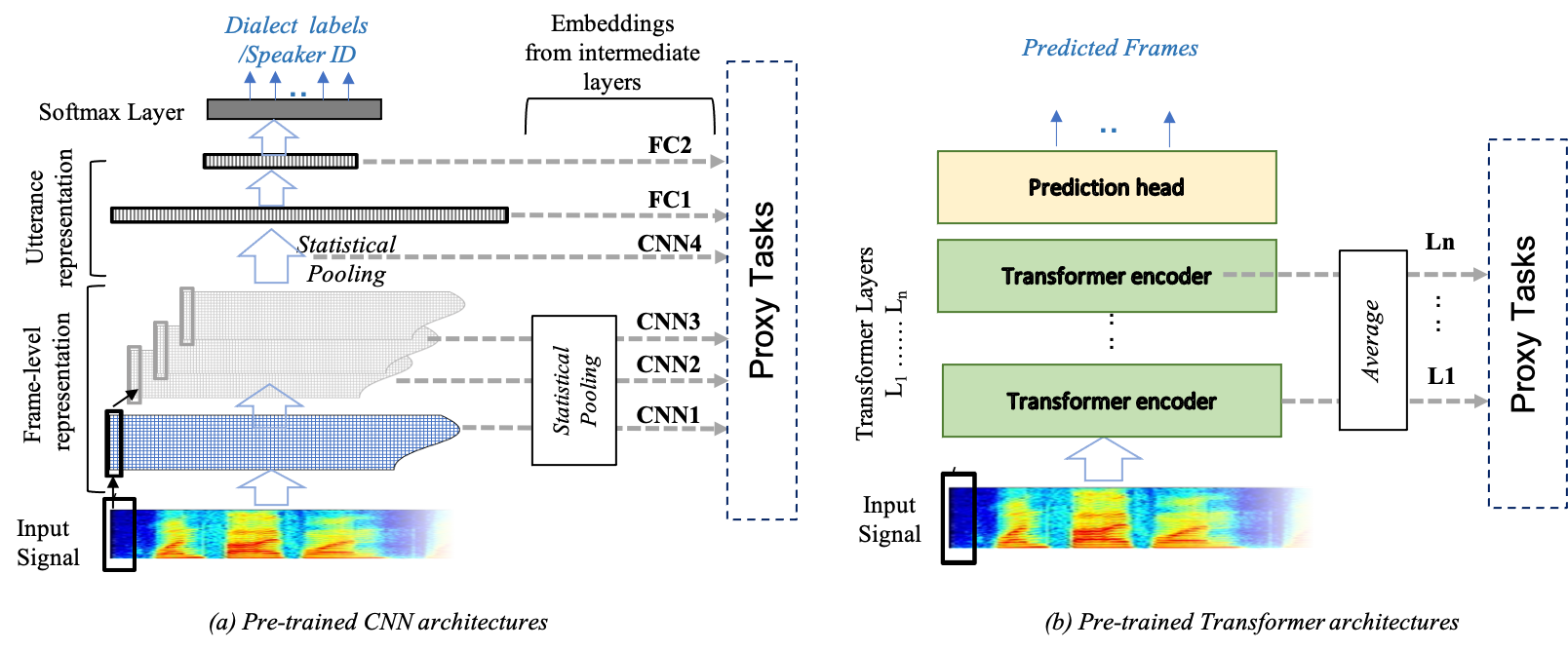
Figure 2: Architecture of the pretrained models. Figure 2a presents the CNN and Figure 2b presents the transformer architecture. FC - fully-connected layer, CNN - convolution layer.

4 Experimental Setup

4.1 Pretrained Models

We experimented with a temporal Convolutional Neural Network (CNN) trained with two different objective functions and two Transformer architectures (refer to Sections 4.1.1 and 4.1.2). The choice of architectures is motivated by the effectiveness of CNNs in modelling different speech phenomena, as well as the increasing popularity and state-of-the-art performance of Transformers in speech and language modeling.

4.1.1 CNN

The CNN models, as illustrated in Figure 2a, comprise four temporal CNN layers followed by two feed-forward layers. These models are specifically optimized for two tasks: i) Arabic dialect identification (ADI) and ii) speaker recognition (SR). Dialectal Arabic is used in 22 countries, with over 20 mutually incomprehensible dialects and a shared phonetic and morphological inventory, making Arabic Dialect Identification particularly challenging when compared to other dialect identification tasks [85]. The model is trained using the Arabic Dialect Identification 17 (ADI17) dataset [86, 87]. We conducted experiments on speaker recognition task using English (SRE). We adapted the approach from [88] and trained the model using the Voxceleb1 development set, which includes data from 1211 speakers and approximately 147K utterances.

4.1.2 Transformer

We included two transformer-encoder architectures using Mockingjay [11], of which we tried two variations differing in the number of encoder layers (3 or 12 – see Figure 2b). We refer to the former as base ($ST_{base}$) and the latter as large ($ST_{large}$) models. The base model ($ST_{base}$) is trained using Mel features as the reconstruction target, whereas for the large model ($ST_{large}$) we use a linear-scale spectrogram as the reconstruction target. The models were trained using the LibriSpeech corpus:train-clean-360.

4.2 Proxy Tasks

We conducted experiments in our study using the following proxy tasks: i) Gender Classification, ii) Speaker Verification, iii) Language Identification, iv) Regional Dialect Classification, and v) Channel Classification. Below, we provide brief details related to each of these tasks.

T1 - Gender Classification (GC)

For the gender classification task, we trained proxy classifiers using the VoxCeleb1-test [17] (English) dataset, which includes videos of celebrities from different ethnicities, accents, professions, and ages. We used gender-balanced train and test sets with no overlapping speakers. The detailed label distribution for the task is shown in Figure 3(a).

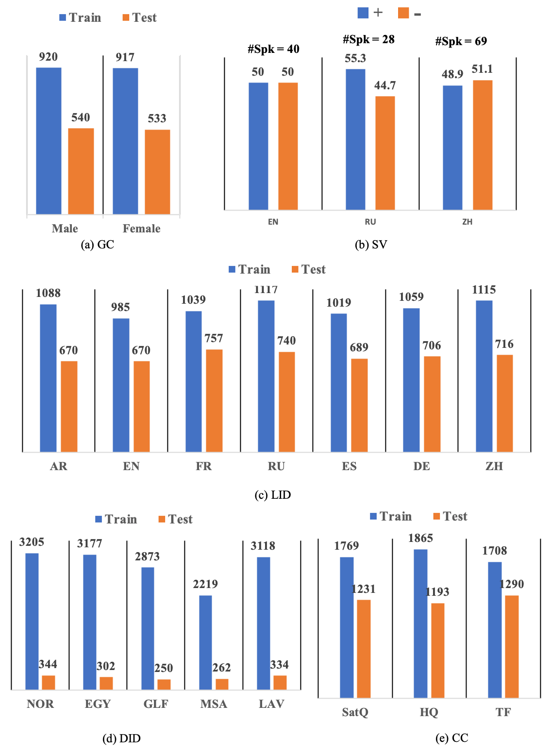
Figure 3: Train and Test Data distribution for proxy classification tasks. Figure 3(a) shows data distribution for GC – Gender Classification (Task1). Figure 3(b) SV – Speaker Verification (Task2): the blue bar represents the positive (from the same speaker) label and the orange is the negative label (from different speaker pairs). $\#Spk$ represents the total number of speakers in each class label ($+/-$) for English EN, Russian RU, and Chinese ZH data. Figure 3(c) LID – Language Identification (Task3); Figure 3(d): DID – Regional Dialect Identification (Task4); and Figure 3(e): CC – Channel Classification (Task5). For Figure 3(a, c-e), the x-axis indicates the class labels whereas the y-axis of each bar chart represents the frequency of the corresponding class.

T2 - Speaker Verification (SV)

We conducted two experiments for the speaker verification task, focusing on two aspects. Firstly, we investigated the presence of voice identity information in different layers of the network. Secondly, we aimed to identify the minimum subset of neurons that could effectively encode voice identity. For the first experiment, we performed a “generic speaker verification” task using pairs of input signals, where we verified if two utterances are from the same or different speaker. For each input signal pair, we extracted length-normalized embeddings from individual layers of the network, as well as their combination (referred to as “ALL”). Subsequently, we computed the cosine similarity between the pairs to analyze the results.

In the second experiment, we conducted a neuron-level analysis by training a proxy classifier for speaker recognition using embeddings from layers of pretrained models. We employed an algorithm detailed in Section 3.3.2 to select the minimal neurons, which were then used to test our verification pairs. The proxy speaker recognition model was trained on the VoxCeleb2-test set [89], which consists of $118$ speakers, $4,911$ videos, and $36,237$ utterances.

In our speaker verification tasks, we utilized a multi-lingual subset of the Common Voice dataset [90], as well as the official verification test set (Voxceleb1-tst) from VoxCeleb1 [17]. The Common Voice corpus is an extensive collection of over $2,500$ hours of speech data in approximately $39$ languages. It was collected and validated through a crowdsourcing approach, making it one of the largest multilingual datasets available for speech research. The data was recorded using a website or an iPhone application provided by the Common Voice project. For our experiments, we selected three languages: English (EN), Russian (RU), and Chinese (ZH), and used the Voxceleb1-tst dataset along with a randomly selected subset of Common Voice data, totaling approximately $4$ hours.

T3 - Language Identification (LID)

We developed classifiers to discern between 7 different languages from the Common Voice dataset for the language identification task. The languages included in our study are Arabic (AR), English (EN), Spanish (ES), German (DE), French (FR), Russian (RU), and Chinese (ZH). The distribution of the datasets for training and testing the classifiers can be seen in Figure 3(c).

T4 - Regional Dialect Classification (DID)

To train our regional dialect classification model, we utilized the Arabic ADI-5 dataset [91], which comprises five dialects: Egyptian (EGY), Levantine (LAV), Gulf (GLF), North African Region (NOR), and Modern Standard Arabic (MSA). The dataset includes satellite cable recordings (SatQ) in the official training split, as well as high-quality (HQ) broadcast videos for the development and test sets. We designed the proxy task using the balanced train set and evaluated the model using the test split. Figure 3(d) provides detailed information on the class distribution.

T5 - Channel Classification (CC)

In our study on Channel Classification, we utilized two datasets: ADI-5 [91] and CALLHOME [92, 93]. Our multi-class classifier assigns labels to indicate the input signal quality, which can be Satellite recording (SatQ), high-quality archived videos (HQ), or Telephony data (TF). To create the SatQ data, we used the ADI-5 train data, while the HQ data was built using the ADI-5 development and test sets. For the TF data, we upsampled the CALLHOME data to a 16kHz sampling rate. We employed a Voice Activity Detector (VAD) to segment the conversations into speech segments and then randomly selected segments with a duration exceeding 2.5 seconds. To conduct the proxy task, we randomly selected balanced samples from each class and divided them into train and test sets using a 60-40% split for our experiment. The dataset distribution is visualized in Figure 3(e).

4.3 Classifier Settings

We trained logistic regression models with elastic-net regularization, using the Adam optimizer with a default learning rate, for 20 epochs and a batch size of 128. The classifier was trained by minimizing the cross-entropy loss. We used fixed values for $\lambda_{*}$ ($\lambda_{*}=0$ and $\lambda_{*}=1e-5$) in our experiments.

5 Layer-wise Analysis

In our initial analysis, we focus on the outcomes obtained from training layer-wise proxy classifiers, aiming to address two key questions: i) does the end-to-end speech model capture distinct properties, and ii) which specific components of the network primarily contribute to learning these properties? To gain insights, we utilize multiple reference points for observations.

5.1 Majority Baseline, Oracle and Control Tasks

Table 1 presents the results of various tasks. We start by comparing against the majority baseline (‘Maj-C’), which predicts the most frequent class in the training data for all instances in the test data. To assess the presence of knowledge in our network, we train a classifier on the concatenation of all network layers (‘ALL’).

Our observations show that the classifier trained on the feature vectors generated from the network (‘ALL’) outperforms the majority baseline (‘Maj-C’) significantly, indicating that our network has acquired meaningful knowledge regarding the understudied properties. To further confirm that our probe is not simply memorizing, we compare against classifiers trained using random vectors (‘R.INIT’) and compute selectivity results [81]. Notably, the classifier trained on random vectors performs similarly or worse than the majority baseline. The high selectivity numbers (‘$Sel_{a}$’) provide evidence that the representations generated by our model truly reflect the acquired properties and are not just artifacts of memorization. With the effectiveness of our results established, we can now conduct a detailed discussion of the individual properties and perform a comprehensive layer-wise analysis to gain a deeper understanding of our findings.

	ADI	SRE	$ST_{base}$	$ST_{large}$
$\#Neurons$	11100	11100	2304	9216
T1: GC — labels# 2
	ADI	SRE	$ST_{base}$	$ST_{large}$
$Acc$ (Maj-C)	56.70
$Acc$ (ALL)	98.20	96.79	99.16	98.14
$Acc$ (R.INIT)	68.14	68.14	56.17	56.60
$Sel_{a}$	42.78	67.28	52.83	72.53

	ADI	SRE	$ST_{base}$	$ST_{large}$
$\#Neurons$	11100	11100	2304	9216
T3: LID — labels# 7
	ADI	SRE	$ST_{base}$	$ST_{large}$
$Acc$ (Maj-C)	14.96
$Acc$ (All)	86.00	76.01	57.35	76.24
$Acc$ (R.INIT)	13.20	13.20	15.58	14.23
$Sel_{a}$	75.69	69.20	41.18	61.76

T4: DID — labels# 5
	ADI	SRE	$ST_{base}$	$ST_{large}$
$Acc$ (Maj-C)	23.06
$Acc$ (ALL)	55.63	39.12	36.66	39.22
$Acc$ (R.INIT)	20.24	20.24	16.70	22.45
$Sel_{a}$	36.7	16.89	13.34	19.20

T5:CC — labels# 3
	ADI	SRE	$ST_{base}$	$ST_{large}$
$Acc$ (Maj-C)	32.12
$Acc$ (ALL)	93.93	85.51	86.80	96.55
$Acc$ (R.INIT)	26.52	28.54	37.74	37.32
$Sel_{a}$	63.81	77.65	68.17	83.76

Table 1: Reported accuracy (Acc) for the proxy Tasks T1: GC, T3:LID, T4:DID and T5:CC using majority baseline (Maj-C), Oracle (ALL: with all neurons), random initialisation (R.INIT) of neuron’s weight and selectivity ($Sel_{a}$). — labels# represent the number of labels in the task. Reported performance are averaged over 5 runs. The standard deviation for the ALL results are presented in Table 8.

5.2 Encoded Properties

In this section, we present our findings from the layer-wise analysis. We trained individual classifiers using the feature vectors obtained from each layer separately. This approach allows us to conduct a comprehensive examination of the network on a per-layer basis.

T1: Gender Classification (GC)

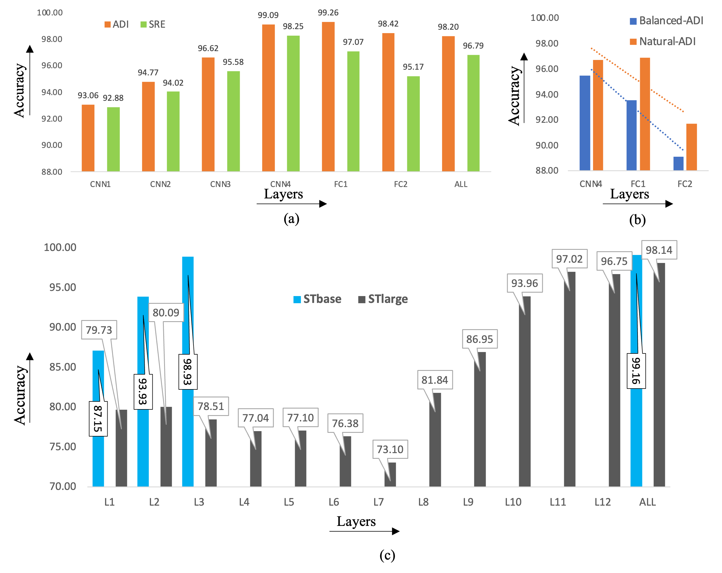
Figure 4: Reported accuracy, for proxy Task Gender classification T1:GC using intermediate network layers. Figure 4a presents the layer-wise performance of ADI and SRE models and Figure 4b presents results for the last 3 layers from a similar ADI architecture, trained with balanced (Balanced-ADI) and natural (Natural-ADI) distribution of gender labels for 4 dialects. Figure 4c presents the layer-wise accuracy for $ST_{base}$ and $ST_{large}$. Reported performance averaged over 5 runs. Majority baseline (assigning most frequent class): 56.70 accuracy.

Figure 4 reveals that while the upper layers of the network acquire the most knowledge regarding gender, other layers also capture sufficient information, indicating that the property is distributed across the layers. Notably, we observed that the model trained for the ADI task appears to be more susceptible to gender information compared to models trained for other downstream tasks. We hypothesize that this could be attributed to representation bias [94], wherein the ADI model exhibits a bias towards higher-pitched and breathier voices, which are predominantly female, because of the substantial gender imbalance and lack of variability in the training data, with fewer than one-third of speakers being female. On the other hand, the other pretrained models, such as SRE and transformers, do not demonstrate this bias.

To further investigate this hypothesis, we trained two dialect identification models, while maintaining (i) the natural distribution of gender data among dialects, and (ii) a balanced distribution. We then probed these models for gender information using the same approach. Our findings (Figure 4b) reveal that the upper (task-oriented) layers are less susceptible to gender information with the balanced-ADI compared to the natural-ADI. This illustrates how data imbalance in gender representation can impact the performance of speech models, as demonstrated in previous studies such as Speaker Recognition models in [34]. Our layer- and neuron-wise analyses (Section 6.2) identify specific components of the network that exhibit such bias, reflecting the usefulness of our study for addressing bias in the network, such as imbalanced gender representation or other properties. Further exploration in this area is left for future research.

Redundancy: Next, we will illustrate the distribution of redundant information in the network. As a reminder, task-specific redundancy, as highlighted in [84], refers to the parts or features of the network that are redundant with respect to a downstream task. Our findings reveal that, for the CNN architecture, the layers above CNN4 exhibit redundancy in relation to the gender classification task. In other words, the higher layers do not possess features that significantly improve performance on this task beyond 1% compared to the best performing layer. This observation holds true for both SRE and ADI models.

T2: Speaker Verification (SV)

We observed that the majority of the models learn speaker-invariant representations (T2:SV – see Figure 5), resulting in poor performance in the speaker verification task. This demonstrates the model’s robustness towards unknown speakers and its generalization ability. When comparing the performance of the networks, we noticed that only the speaker recognition model (SRE) learned voice identity in the final layers of the network. We also observed a similar pattern when testing the SRE model on other languages, such as Chinese and Russian, indicating the domain and language-agnostic capability of the SRE model (See Figure5).

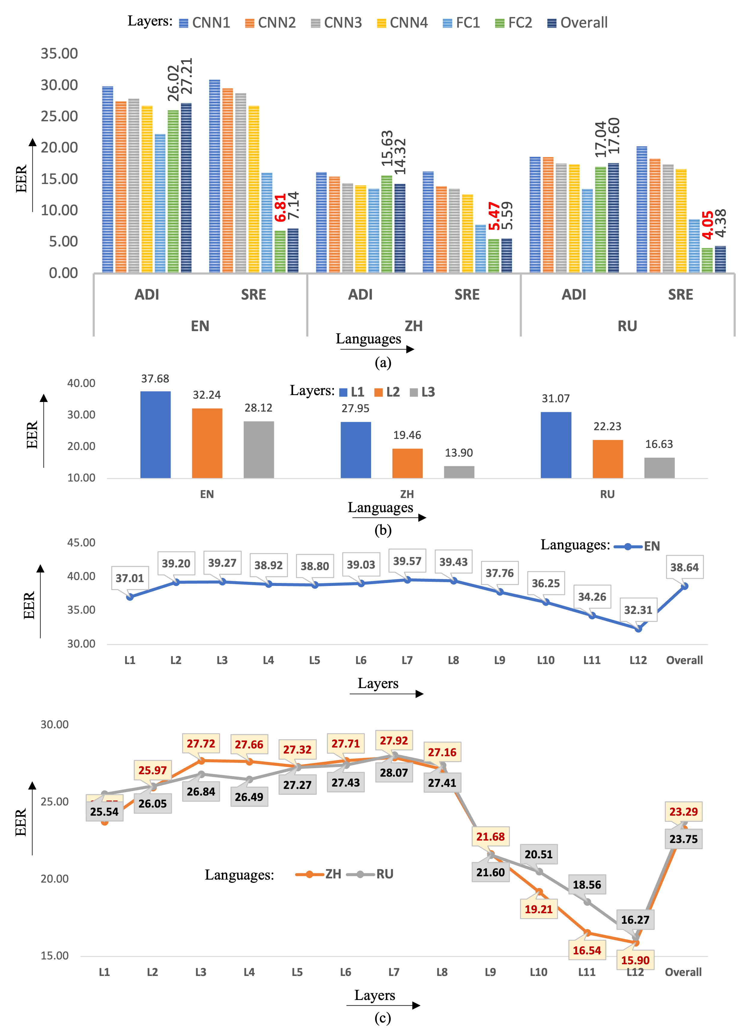
Figure 5: Reported Equal Error Rate (EER) for proxy Speaker verification, Task T2:SV using intermediate network layers. Figure 5a presents the layer-wise performance of ADI and SRE models for EN, ZH and RU languages, the best EER are represented in red color. Figure 5b-c presents the layer-wise EER for $ST_{base}$ and $ST_{large}$. For a better visibility, Figure 5c is divided into two graphs for the reported languages (EN - blue, ZH - orange and RU - grey curve). EER value, the lower the better.

T3: Language Identification (LID)

Our findings reveal that language markers are predominantly encoded in the upper layers of most of the studied models, particularly in the second-to-last layer (as shown in Figure 6a). The upper layers primarily contain task-related information, as evidenced in T2:SV and later in T4:DID. Therefore, the presence of language information in these layers suggests their significance in discriminating between speakers or dialects. Furthermore, our results highlight that self-supervised models also capture language information as subordinate information during the encoding of the input signal.

When comparing architectures, we noticed that the CNN outperformed the transformer in capturing language representations (discussed further in detail in Section 6.3). Additionally, we observed that the ADI model demonstrated significantly better performance in our probing task, particularly when using the CNN4 layer. This highlights that the model, which is originally designed to distinguish between dialects, is also proficient in discriminating languages and can be effectively fine-tuned for language identification tasks.

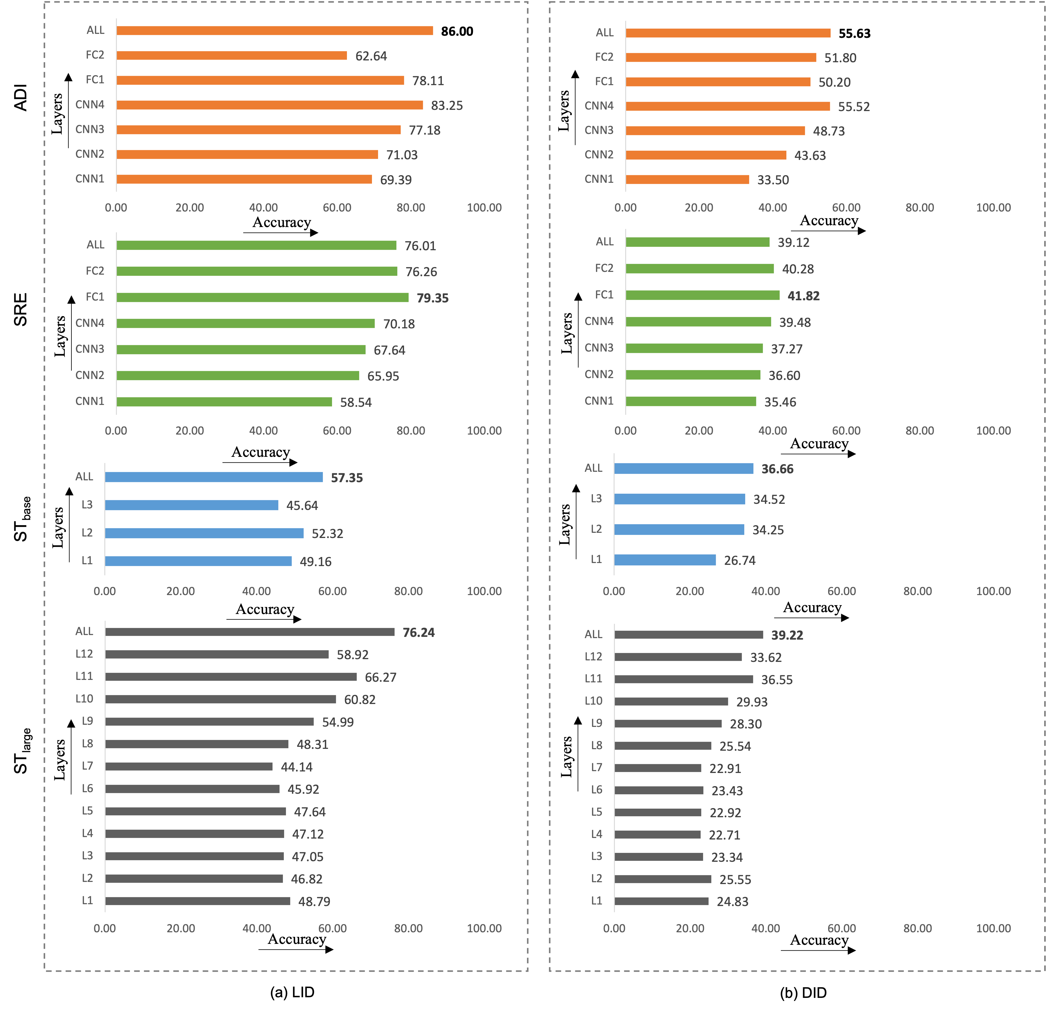
Figure 6: Reported Accuracy for proxy Tasks T3:LID and T4:DID using intermediate network layers. Figure 6a presents the layer-wise performance of all the pretrained models for the language identification task and Figure 6b presents the layer-wise accuracy for the dialect identification task. Reported performance averaged over 5 runs. Majority baseline: T3 - 14.96 and T4 - 23.06 accuracy.

T4: Regional Dialect Identification (DID)

During our investigation of regional dialectal information, we discovered that most of the networks failed to capture the discriminating properties of dialectal information, as illustrated in Figure 6b. This reflects the complexity of distinguishing between different dialects. However, we observed that the task-specific model ADI was able to successfully capture the dialectal variation in the upper layers (CNN4-FC2) of the network. This suggests that the original pretrained models do not capture sufficient information for this complex task and that task-specific supervision is necessary to achieve accurate results, which are then preserved in the upper layers of the model.

T5: Channel Classification (CC)

Similar to the gender information task (T1:GC), we observed that channel information (as shown in Figure 7) is consistently present throughout all layers of the network. This indicates that the network is capable of generalizing well on mixed data that includes varying environments, such as differences in microphones and data sources (e.g. broadcast TV, YouTube, among others). The network’s ability to perform consistently across all layers on this task demonstrates its robustness in handling data with diverse channel characteristics.

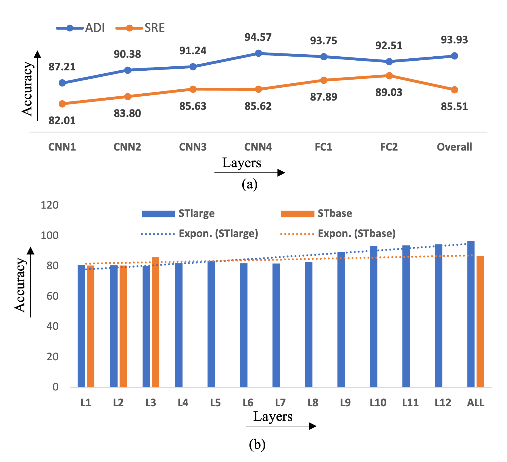
Figure 7: Channel classification layer-wise Accuracy. Reported performance averaged over 5 runs. The dotted lines (Figure 7b) show the trend-line of the graphs. Majority baseline (assigning most frequent class): 32.12 accuracy.

5.3 Summary

Our analysis of the pretrained networks revealed several key findings: i) channel and gender information are encoded and distributed throughout the networks at different layers, ii) gender information is redundantly encoded in both the ADI and SRE pretrained models, iii) the ADI network shows a higher susceptibility to gender-based representation bias compared to other models, iv) all pretrained models, except for SRE, learn speaker-invariant representations, v) voice identity is only encoded in the upper layers of the SRE model, vi) language properties are captured in the upper layers of all pretrained models, vii) pretrained models trained for dialect identification are well-suited for knowledge transfer in language identification downstream tasks, viii) regional dialectal information is only captured in the task-specific network (ADI) in the upper layers of the network (task-layers), unlike language properties.

6 Neuron Analysis

In this section, we conduct a detailed analysis of representations at the neuron level. The section is divided into two parts: i) evaluating the effectiveness of the neuron ranking algorithm, and ii) drawing task-specific and architectural comparisons based on the identified neurons.

	ADI	SRE	$ST_{base}$	$ST_{large}$
$Neurons$	20%	20%	20%	20%
T1: GC — labels# 2
	ADI	SRE	$ST_{base}$	$ST_{large}$
$Acc_{t}$ (Masked)	98.23	97.58	95.43	93.65
$Acc_{b}$ (Masked)	53.36	58.65	77.13	55.87
$Acc_{r}$ (Masked)	98.06	87.08	95.93	92.64

	ADI	SRE	$ST_{base}$	$ST_{large}$
$Neurons$	20%	20%	20%	20%
T3: LID — labels# 7
	ADI	SRE	$ST_{base}$	$ST_{large}$
$Acc_{t}$ (Masked)	65.38	64.89	50.45	70.51
$Acc_{b}$ (Masked)	16.30	17.26	21.13	17.14
$Acc_{r}$ (Masked)	58.83	42.94	48.40	58.84

T4: DID — labels# 5
	ADI	SRE	$ST_{base}$	$ST_{large}$
$Acc_{t}$ (Masked)	52.75	31.29	23.14	36.21
$Acc_{b}$(Masked)	22.33	23.67	24.21	22.40
$Acc_{r}$ (Masked)	34.01	25.78	24.97	29.05

T5:CC — labels# 3
	ADI	SRE	$ST_{base}$	$ST_{large}$
$Acc_{t}$ (Masked)	88.60	86.48	79.40	88.69
$Acc_{b}$ (Masked)	41.00	36.64	49.69	33.14
$Acc_{r}$ (Masked)	87.49	75.36	80.28	88.87

Table 2: Reported accuracy (Acc), to indicate neuron ranking and selection algorithm efficacy for the proxy Tasks T1: GC, T3:LID, T4:DID, and T5:CC using Masked 20% t/b/r neurons. $Acc_{*}$ with t=top, b=bottom and r=random. The rankings are based on the absolute values of the weights. — labels# represent the number of labels in the task. Reported performances are averaged over 5 runs.

6.1 Efficacy of the Neuron Ranking

First, we evaluate the effectiveness of the neuron selection algorithm by recomputing the classifier accuracy after masking out 80% of the neurons and retaining the top/random/bottom 20% neurons. Please refer to Tables 2 for results on different tasks (T1,3-5). Our findings reveal that the top neurons consistently yield higher accuracy compared to the bottom neurons, demonstrating the efficacy of the ranking algorithm.

6.2 Minimal Neuron Set

To analyze individual neurons, we extract a minimal subset of neurons for each task. We rank neurons using the algorithm described in Section 3.3 with the goal of achieving comparable performance to the oracle (within a certain threshold). Table 3 presents the minimal number of neurons extracted for each task. We discuss the results for different tasks below and also utilize the minimal set of neurons for redundancy analysis (Section 3.5). Specifically, we define task-specific redundancy as follows: i) if the minimal set of neurons achieves at least 97% of the oracle performance, then the remaining neurons are considered redundant for this task, ii) if randomly selected N% of neurons also achieve the same accuracy as the top N% neurons, we consider the information redundant for this task.

T1: GC — labels# 2
	ADI	SRE	$ST_{base}$	$ST_{large}$
$Acc$ (ALL)	98.20	96.79	99.16	98.14
$Neu_{t}$	5%	50%	15%	10%
$Acc_{t}$ (Re-trained)	98.68	96.54	98.32	98.14
$Acc_{r}$ (Re-trained)	94.65	95.28	97.44	87.99

T3: LID — labels# 7
	ADI	SRE	$ST_{base}$	$ST_{large}$
$Acc$ (All)	86.00	76.01	57.35	76.24
$Neu_{t}$	20%	10%	75%	50%
$Acc_{t}$ (Re-trained)	85.30	78.97	57.45	76.43
$Acc_{r}$ (Re-trained)	82.46	70.00	55.68	72.53

T4: DID — labels# 5
	ADI	SRE	$ST_{base}$	$ST_{large}$
$Acc$ (ALL)	55.63	39.12	36.66	39.22
$Neu_{t}$	25%	5%	50%	15%
$Acc_{t}$(Re-trained)	55.43	40.82	36.01	38.06
$Acc_{r}$ (Re-trained)	50.32	37.52	33.45	31.45

T5:CC — labels# 3
	ADI	SRE	$ST_{base}$	$ST_{large}$
$Acc$ (ALL)	93.93	85.51	86.80	96.55
$Neu_{t}$	10%	1%	20%	10%
$Acc_{t}$ (Re-trained)	94.56	85.04	86.27	95.71
$Acc_{r}$ (Re-trained)	92.82	75.85	84.70	92.49

Table 3: Reported re-trained accuracy (Acc) with minimal neuron set for proxy Tasks T1,T3,T4 and T5. $Acc_{*}$ with t=top, and r=random Neu: neurons. — labels# represent the number of labels in the task. Reported performances averaged over 5 runs.

T1: Gender Classification (GC)

We have observed that a small set of neurons (5-15%) is sufficient to achieve accuracy close to the oracle performance ($Acc(ALL)$) with an accuracy difference of within 97%. Furthermore, in most of the pretrained models, we have observed a small accuracy difference (within a threshold of 5%) between the top and random subsets. This indicates that the information of gender is redundantly available throughout the network.

In the SRE model, we have observed a drop in probe accuracy when retrained with the top 50% neurons, as compared to the masked accuracy and the oracle (‘ALL’) accuracy, as shown in Table 2. We speculate that this behavior is influenced by the nature of the pretrained model and its training objective. The primary objective of the pretrained SRE model is to discriminate speakers, where gender recognition is crucial information for such discrimination. Therefore, the gender classification probe trained with all the neurons of the pretrained network outperforms the probe with minimal neurons, indicating that the gender property is not redundant in the SRE model, and the neurons capture some variant information. This hypothesis is supported by the comparison of the cardinality of the minimal neuron set in the SRE model (50% neurons) versus the other pretrained models (5-15% neurons).

EER	$L_{b}$	$EER(L_{b})$	$Neu_{t}$	$EER_{t}$	$EER_{r}$	$EER_{b}$
EN
ADI	FC1	22.27	75%	22.03	22.32	22.50
SRE	FC2	6.81	75%	6.96	6.96	7.05
$ST_{base}$	L3	28.12	5%	27.57	31.04	32.43
$ST_{large}$	L11	32.31	5%	26.64	34.11	39.36
ZH
ADI	FC1	13.55	50%	14.37	15.85	14.51
SRE	FC2	5.47	50%	6.06	6.56	6.10
$ST_{base}$	L3	13.90	20%	13.78	15.19	20.49
$ST_{large}$	L11	15.90	5%	15.62	15.06	26.29
RU
ADI	FC1	13.47	50%	12.81	14.09	14.66
SRE	FC2	4.05	50%	4.59	4.41	4.93
$ST_{base}$	L3	16.63	10%	16.25	16.75	19.29
$ST_{large}$	L11	16.27	10%	9.09	15.04	24.44

Table 4: Reported equal error rate (EER) for proxy Task T2:SV using fine-grained neuron analysis. $EER_{*}$ with t=top, b=bottom and r=random Neu: neurons. $L_{b}$ represent the best layer from the pretrained model with lowest EER. $Neu_{t}$ represent percentage of neurons selected. Reported performance averaged over 5 runs.

T2: Speaker Verification (SV)

In on our layer-wise results, we have observed that the speaker-variant information is only present in the last layer of the speaker recognition (SRE) model. Upon further studying the represented layer ($L_{b}$), we have noticed that approximately 75% (EN) of the neurons in the last layer are utilized to represent this information, as shown in Table 3.

When comparing top neurons to random neurons in SRE, we found that the equal error rate (EER) of the random set (6.96) is the same as the EER of the top set (6.96). However, the minimal representation obtained from the top set does not outperform the complete FC2 neuron set. This result indicates that all neurons in FC2 are relevant to the tasks.

T3: Language Identification (LID)

In contrast to the pretrained speech transformers, the CNN models require a small neuron set (10-20% of the total network) to encode the language property, as shown in Table 3. Additionally, we observed that approximately 80% of neurons are redundant for the language property only in the ADI model. We hypothesize that this redundancy is due to the nature of the task and the training objective of the model. Since the core task of ADI is to discriminate dialects, a small number of pretrained model neurons are sufficient to store the knowledge related to the language property.

T4: Regional Dialect Identification (DID)

The layer-level analysis revealed that the ADI model captures dialectal information only in the representations learned within its network. This observation was further confirmed in the neuron analysis. Table 3 demonstrates that using only 25% of the neurons from the ADI network, the probe achieves a comparable accuracy to the ’ALL’ neuron set ($Acc(ALL)$). However, it’s important to note that re-training the classifier with a random 25% of neurons did not achieve the oracle accuracy within the accepted threshold. This suggests that, unlike other properties, the dialectal information is not redundant in the ADI network.

Layers	CNN1	CNN2	CNN3	CNN4	FC1	FC2
#Neu/Layers	2000	2000	2000	3000	1500	600
#Neu (total)	11100
Tasks ($Neu_{t}$ %)	Network: ADI
LID (20)	0 (0.0%)	153 (1.4%)	0.4 (0.0%)	576.6 (5.2%)	1034.2 (9.3%)	455.8 (4.1%)
DID (25)	0 (0.0%)	162.2 (1.5%)	0.2 (0.0%)	776.8 (7.0%)	1264.2 (11.4%)	571.6 (5.1%)
GC (5)	0 (0.0%)	10.6 (0.1%)	1 (0.0%)	74.8 (0.7%)	329.8 (3.0%)	138.8 (1.3%)
CC (10)	0.8 (0.0%)	63.6 (0.6%)	4 (0.0%)	184 (1.7%)	608.8 (5.5%)	248.8 (2.2%)
Tasks ($Neu_{t}$ %)	Network: SRE
LID (10)	25.8 (0.2%)	104.2 (0.9%)	102 (0.9%)	36.8 (0.3%)	577.2 (5.2%)	264 (2.4%)
DID (5)	28.8 (0.3%)	47.8 (0.4%)	56 (0.5%)	35.8 (0.3%)	382.2 (3.4%)	4.4 (0.0%)
GC (50)	938.2 (8.5%)	948.8 (8.5%)	936.4 (8.4%)	1394.8 (12.6%)	838 (7.5%)	493.8 (4.4%)
CC (1)	0 (0.0%)	0.4 (0.0%)	0 (0.0%)	0.6 (0.0%)	69.4 (0.6%)	40.6 (0.4%)

Table 5: Distribution of top neurons across the ADI and SRE network for each task. Reported number of neurons averaged over 5 runs.

T5: Channel Classification (CC)

We observed that a small percentage (1-20%) of neurons are capable of representing the property while achieving accuracy comparable to $Acc$(ALL), as shown in Table 3. This finding highlights the pervasive nature of the channel information. Furthermore, our analysis of re-trained top and random accuracy revealed that a substantial number of neurons are redundant for representing channel information in most of the pretrained network.

6.3 Localization vs Distributivity

Now we highlight the parts of the networks that predominantly capture the top neurons properties. We present the distribution of the top salient (minimal) neurons across the network in Table 5-7, to study how distributed or localized the spread of information is.

	Network: $ST_{base}$
Tasks ($Neu_{t}$ %)	L1	L2	L3
LID (75)	605 (26.3%)	556.6 (24.2%)	566.4 (24.6%)
DID (50)	273.2 (11.9%)	582.4 (25.3%)	296.4 (12.9%)
GC (15)	42.4 (1.8%)	137.2 (6.0%)	165.4 (7.2%)
CC (20)	124.2 (5.4%)	231 (10.0%)	104.8 (4.5%)

Table 6: Distribution of top neurons across the $ST_{base}$ network for each task. Number of neurons in each layer = 768. Total neurons (‘ALL’) in the network = 2304. The table reports the number of neurons (#) in each layer which is a member of $Neu_{t}$%. Each cell also reports the % the selected neurons represents wrt to the ‘ALL’ neurons in the network. Reported number of neurons averaged over 5 runs.

T1: Gender Classification (GC)

Tables 5-7 show that the salient neurons (e.g., 5% of ADI network) for the gender property are predominantly present in the upper layers of the network. This finding is consistent with our previous analysis of task-specific layer- and neuron-level minimal sets, which indicates that the information is redundantly distributed. It suggests that using a small set of neurons from any part of the network (as shown in Table 3 Acc_r) can yield results that are close to using the entire network.

T2: Speaker Verification (SV)

We observed from the minimal set analysis of the SRE pretrained model that a majority of the neurons (approximately 75% in EN) in the last layer are needed to represent the information. This indicates that the information is distributed throughout the last layer, which aligns with our layer-wise observation. Furthermore, we also found that these salient neurons are shared with other properties, such as gender, in a similar manner as observed in Chinese and Russian datasets.

Network: $ST_{large}$
Layers	Tasks ($Neu_{t}$ %)
	LID (50)	DID (15)	GC (10)	CC (10)
L1	423.6 (4.6%)	26.2 (0.3%)	11 (0.1%)	13.2 (0.1%)
L2	171 (1.9%)	7.2 (0.1%)	6.2 (0.1%)	3 (0%)
L3	124 (1.3%)	10.4 (0.1%)	2.4 (0%)	5.2 (0.1%)
L4	153 (1.7%)	11.4 (0.1%)	2.6 (0%)	124.4 (1.3%)
L5	247.6 (2.7%)	50.4 (0.5%)	12 (0.1%)	129.8 (1.4%)
L6	266.8 (2.9%)	33.2 (0.4%)	3.2 (0%)	28.6 (0.3%)
L7	305.6 (3.3%)	53.4 (0.6%)	10.8 (0.1%)	23 (0.2%)
L8	327.6 (3.6%)	64.6 (0.7%)	9.8 (0.1%)	14.2 (0.2%)
L9	615.6 (6.7%)	175.4 (1.9%)	74.6 (0.8%)	58.4 (0.6%)
L10	662.2 (7.2%)	337.2 (3.7%)	227.6 (2.5%)	146 (1.6%)
L11	686 (7.4%)	378.8 (4.1%)	284 (3.1%)	159 (1.7%)
L12	625 (6.8%)	233.8 (2.5%)	276.8 (3%)	216.2 (2.3%)

Table 7: Distribution of top neurons across the $ST_{large}$ network for each task. Number of neurons in each layer = 768. Total neurons (‘ALL’) in the network = 9216. The table reports the number of neurons (#) in each layer which is a member of $Neu_{t}$%. Each cell also reports the % the selected neurons represents with respect to the ‘ALL’ neurons in the network. Reported number of neurons averaged over 5 runs.

T3: Language Identification (LID)

For the language property, the information is more distributed in the pretrained transformers (see Table 6-7), and localised in the upper layers for CNNs (see Table 5). We hypothesize that this difference in behavior is due to the contrasting training objectives of the models, with CNNs trained with task-related supervision and Transformers trained with self-supervision. Both CNN pretrained models, ADI and SRE, are trained with objectives that involve language identification or discrimination as an innate criterion/feature for model prediction. As a result, the neurons in the upper layers of CNNs capture more language-representative information compared to their predecessors.

T4: Regional Dialect Identification (DID)

Based on the minimal set analysis, we observed that only 25% of the neurons in the ADI network are necessary to encode the regional dialects. Further analysis, as presented in Table 5-7, reveals that the regional dialectal information is predominantly localized in the upper layers of the ADI network.

T5: Channel Classification (CC)

We found that salient neurons are localized in the upper layers of CNNs, as shown in Table 5. On the other hand, in transformers, the information is distributed across the middle and upper layers, as evidenced by Table 6-7.

6.4 Summary

Our neuron analysis reveals several key findings: i) it is possible to extract a minimal set of neurons that effectively represent the encoded information, ii) complex tasks, such as voice identity, require a larger number of neurons to encode the information compared to simpler tasks, such as gender classification, iii) network redundancy is observed for simple tasks, such as gender and channel identification, indicating that task-specific information is stored redundantly, iv) for complex tasks, such as dialect and speaker voice verification, the information is not redundant and is only captured by the task-specific network, and v) for most properties, the salient minimal neurons are localized in the upper layers of the pretrained models.

7 Discussion

7.1 Key Observation from Layer and Neuron-level Analysis:

Number of neurons and the task complexity:

We observed that simple properties, such as gender and channel, can be captured with fewer neurons (as little as 1% of the network) to encode the information. One possible explanation could be the nature of the tasks, as gender and channel information are salient and easily distinguishable in the acoustic signal, requiring only a few neurons for accurate classification. On the other hand, for more complex properties, like voice identity verification, a significant number of neurons are necessary to represent the variability in the signal.

Localized vs Distributive:

We observed that the salient neurons for most tasks are concentrated in the upper layers of the pretrained models. This observation is particularly evident in the voice identity verification task of the SRE model, where nearly 50-75% of neurons in the last layer encode such information. We hypothesize that neurons in each successive layer are more informative than their predecessors, and as we delve deeper into the network, more contextual information is captured, aiding in discriminating factors like variability in a speaker’s voice.

Task-specific Redundancy:

We noticed task-specific redundancy at both the layer and neuron levels for gender and channel properties. This redundancy arises due to the distinct acoustic signature of these properties, which allows for the learning of redundant information across the network, often represented by a small number of neurons. In addition, we also observed neuron-level redundancy for the language property in the ADI model. We hypothesize that a limited number of neurons are sufficient to capture the variability between languages when transferred from the pretrained model, which is originally trained to distinguish dialects within a language family.

Polysemous Neurons:

We observed that salient neurons are sometimes shared across different properties. For instance, in the SRE pretrained model, we noticed that approximately 40% of the voice-identity neurons are also shared with the gender neurons. This sharing of properties among neurons reflects the main training objective of the pretrained model, which is to recognize speakers, as both gender and voice variability are essential for verifying speakers’ identity. Therefore, when creating speaker verification pairs to evaluate the performance of a speaker recognition model, we tend to select pairs from the same gender, to mitigate the influence of gender-based discrimination.

Bias:

Our analysis of fine-grained neurons reveals the presence of property-based representation bias in the pretrained network, shedding light on the specific parts (neurons) that encode information. For instance, through layer and neuron-level analysis, we demonstrate that the ADI pretrained model exhibits a higher susceptibility to gender representation bias compared to other pretrained models. By identifying neurons that capture gender-related information in the network, we can potentially manipulate and control the system’s behavior to eliminate the bias. However, we leave further exploration of this topic for future research

Robustness:

Through our diagnostic tests, we observed that the pretrained networks are robust towards unknown speakers. This increases the reliability of predictions made by the pretrained models. Furthermore, leveraging this information, we can identify potential parts of the network that are susceptible to capturing identity information, and selectively fine-tune only those parts of the pretrained model for any future speaker-dependent downstream tasks, thereby reducing computational costs.

7.2 Cross-architectural Comparison:

Network Size and its Encoding Capabilities:

In comparing pretrained models across different architectures, we observed that classifiers trained from feature representations of smaller transformers exhibit lower performance towards certain concepts that we studied. On the other hand, larger models tend to learn richer feature representations. It is worth noting that the presence of these features is independent of the performance of these models on their actual task, as determined by the loss function they are trained on. Assessing whether these features actually improve performance on the intended task for which the models were trained falls beyond the scope of this paper.

Storing Knowledge:

Our observations reveal a tetrahedral pattern in the storage of knowledge, indicating that deeper neurons in the network tend to be more informative and store more knowledge compared to their counterparts in lower layers. Specifically, in large architectures such as CNNs and large transformers, we notice that task-oriented information is predominantly captured in the upper layers, encoding more abstract information, while vocal features are primarily captured in the lower layers. These findings corroborate previous studies that suggest the lower layers of the network function as feature extractors, while the upper layers serve as task-oriented classifiers. This observation is also consistent with the results presented in [38], where the authors propose that the representation in the lower layers resembles traditional low-level speech descriptors extracted from classical feature extraction pipelines, such as formants, mean pitch, and voice quality features. However, in the case of small transformer pretrained models, the information is more distributed throughout the network.

Pretrained Architecture for Transfer Learning:

The most popular architecture choice for the pretrain-fine-tune paradigm is transformers, especially in the context of pretrained language modeling and speech representation models. However, within the research community, there is also an abundance of large CNN models that have been trained for various tasks. In line with the findings of [52], our results suggest that there is potential in (re-)using these large CNNs as pretrained models for transferring knowledge to another task, regardless of their original pretraining objectives. Specifically, our findings indicate that reusing these pretrained CNNs can yield comparable or even better performance compared to transformer models, with the added benefit of reduced computational resources

7.3 Potential Applications

There are numerous potential applications for interpreting speech models beyond analyzing and understanding these models. In this section, we will discuss some of these potential applications that can benefit from the findings of this work.

Network Pruning

Neural Networks are inherently redundant due to massive over-parameterization, which results in computational inefficiencies in terms of storage and efficiency. However, numerous techniques have been successful in reducing the computational cost and memory requirements during inference, indicating that not all representations encoded by the rich architecture are necessary. Our neuron and redundancy analysis further reinforces this observation. Firstly, we showed that network layers are redundant with respect to different tasks. We also demonstrated that neurons within these layers are redundant and that a minimalist subset of neurons can be extracted to achieve close to oracle performance on any downstream task. These observations can be leveraged for network pruning, for example, by pruning redundant top-layers of the network to reduce its size. This not only makes the model smaller, but also results in faster inference by reducing the forward pass to the first layer that gives close to oracle performance. A study by [95] also showed that pruning layers in the model is an effective way to reduce its size without significant loss in performance.

Feature-based Transfer Learning

Feature learning has emerged as a viable alternative to fine-tuning based transfer learning in the field of Natural Language Processing (NLP), as shown by [96]. Classifiers with large contextualized vectors suffer from issues such as being cumbersome to train, inefficient during inference, and sub-optimal when supervised data is limited, as highlighted by [97]. To address these problems, selecting a minimal subset of relevant neurons from the network can be a solution. [84] combined layer- and neuron-analysis for efficient feature selection in NLP transformers trained on GLUE tasks [98]. We believe that a similar methodology can benefit speech-based CNN and transformer models, and exploring this frontier is an exciting opportunity.

Model Manipulation

Identifying salient neurons in the model with respect to certain properties can potentially enable controlling the model with respect to that property. For example, [30] identified switch neurons that learned male and female gender verbs in Neural Machine Translation and controlled their activation values at inference to change the system’s output. In Section 5.2, we successfully identified and located the sensitive components of the network that relate to the gender property in ADI. We believe that our neuron analysis has a promising potential in facilitating the editing and manipulation of information in speech models, providing a valuable tool for control and customization.

7.4 Limitations

Complexity of the Probe

From a methodological standpoint, we employed a straightforward logistic regression classifier, chosen for its simplicity in theoretical understanding and widespread use in the literature. However, recent studies [66] have suggested that a deeper classifier may be necessary to capture more subtle encoded knowledge. Linear probes play a crucial role in our approach, as we utilize the learned weights as a proxy to gauge the significance of each neuron. Further exploration of more complex probes is left as a potential avenue for future research.

Dependence on Supervision

We trained our probes using pre-defined tasks and annotations, which enabled us to conduct layer-wise and fine-grained neuron analyses. One limitation of this approach is that our analysis is restricted to pre-defined properties for which annotations are available. To uncover additional information captured within the network, and to determine if machine-learned features align with human-engineered features, further unsupervised analysis is needed. Probing classifiers also have limitations, as the analysis can be biased by the constraints of the annotated data, such as sparsity, genre, etc. To validate our findings, it is crucial to conduct analysis under diverse data conditions. We plan to explore this avenue in future research.

Connecting Interpretation with Prediction

Although probing methods are valuable in analyzing and identifying important information captured within the network, they do not necessarily reveal how this information is utilized by the network during prediction [68]. For instance, to mitigate bias in the system’s output, it is essential to identify neurons that are relevant to the property of interest and determine which of these neurons play a critical role during prediction. By combining these two pieces of information, one can effectively exert control over the system’s behavior with respect to that property. This represents a challenging research frontier that we encourage researchers in speech modeling to explore.

8 Conclusion

In this study, we analyzed intermediate layers and salient neurons, in end-to-end speech CNN and transformer architectures for speaker (gender and voice identity), language (and its variants - dialects), and channel information. We explored the architectures, using proxy classifiers, to determine what information is captured, where it is learned, how distributed or focused their representation are, the minimum number of neurons required, and how the learning behavior varies with different pretrained models.

Our findings suggest that channel and gender information are omnipresent with redundant information, unlike voice identity and dialectal information, and require a small subset (mostly 1-20%) of neurons to represent the information. We observed, for complex tasks (e.g. dialect identification), the information is only captured in the task-oriented model, localised in the last layers, and can be encoded using a small salient (e.g., 25% of the network) neuron set. These salient neurons are sometimes shared with other properties and are indicative of potential bias in the network. Furthermore, this study also suggests, in the era of pretrained models, in addition to popular ‘transformers’, CNNs are also effective as pretrained models and should be explored further.

To the best of our knowledge, this is the first attempt to analyse layer-wise and neuron-level analysis, putting the pretrained speech models under the microscope. In future work, we plan to further extend the study to other available architecture, like autoencoders, with low-level information such as phoneme and grapheme and dig deeper into class-wise properties.

Appendix A

A.1 CNN Architecture

The input to the models is 40 coefficient MFCCs features from a spectrogram computed with a 25ms window and 10ms frame-rate from 16kHz audio. The architecture of the models includes four temporal convolution neural networks (1D-CNNs), followed by a global (statistical) pooling layer to aggregate the frame-level representations to utterance-level representations. For the CNN layers, we used filter sizes of 40$\times$5, 1000$\times$7, 1000$\times$1, 1000$\times$1 with 1-2-1-1 strides and 1000-1000-1000-1500 filters respectively. This utterance-level representation is then passed to two fully connected layers (hidden units: 1500 and 600). We used Rectified Linear Units (ReLUs) as activation functions of the network. The network is trained using the stochastic gradient descent (SGD) optimizer with a learning rate of 0.001.

A.2 Transformer Architecture

The input to the models is Mel-features, which are then transformed into high-level representations. For the transformation, the input is first downsampled to adapt to long input sequences, and then the consecutive frames are stacked into one step. This step reduces the number of frames used in the architecture. These input frames are then projected to a fixed dimension of 768 before passing to a sinusoidal function for encoding position. As a result, these frames passed through multi-layer transformer encoder with multi-head self-attention for left-and-right bidirectional encoding. Each transformer encoder outputs the encoder’s hidden states and has a dimension of 768. The transformers are trained for $50000$ steps with a learning rate of 0.001.

A.3 ADI and SRE Model Performance

The overall performance of the trained ADI model using the official MGB-5 dialect test set [87] are accuracy - $82.0$% and $F_{1}$ - $82.7$%.

To evaluate the SR model performance, we performed speaker verification, using the embedding from the last intermediate layer (second fully-connected layer, FC2) of the SRE model with Voxceleb1 official test verification pairs, obtaining $EER=6.81$.

A.4 Variance in the Oracle Results

To compensate for the randomness in the presented results, we ran each of our experiments 5 times and reported the average results. We noticed the variance in our results is very much insignificant, making the results replicable. We reported the standard variation in the accuracies presented in Table 1 in Table 8.

Acc (ALL)	# Class Labels	ADI	SRE	$ST_{base}$	$ST_{large}$
T1: GC	2	$\pm$ 1.41E-03	$\pm$ 6.36E-03	$\pm$ 5.52E-04	$\pm$ 2.76E-04
T3: LID	7	$\pm$ 3.07E-02	$\pm$ 1.14E-02	$\pm$ 4.38E-04	$\pm$ 1.14E-02
T4: DID	5	$\pm$ 2.50E-02	$\pm$ 1.12E-03	$\pm$ 6.70E-04	$\pm$ 3.00E-04
T5: CC	3	$\pm$ 7.02E-04	$\pm$ 1.35E-03	$\pm$ 7.02E-04	$\pm$ 3.30E-04

Table 8: Reported standard deviation for the average accuracy (over 5 runs) reported in Table 1 for Oracle (ALL: with all neurons). The results are reported for the proxy Tasks T1: GC, T3:LID, T4:DID and T5:CC.

References

- Hupkes et al. [2018] D. Hupkes, S. Veldhoen, W. Zuidema, Visualisation and ‘diagnostic classifiers’ reveal how recurrent and recursive neural networks process hierarchical structure, arXiv preprint arXiv:1711.10203 (2018).
- Deng and Liu [2018] L. Deng, Y. Liu, Deep learning in natural language processing, Springer, 2018.
- Voulodimos et al. [2018] A. Voulodimos, N. Doulamis, A. Doulamis, E. Protopapadakis, Deep learning for computer vision: A brief review, Computational intelligence and neuroscience (2018).
- Amodei et al. [2016] D. Amodei, S. Ananthanarayanan, R. Anubhai, J. Bai, E. Battenberg, C. Case, J. Casper, B. Catanzaro, Q. Cheng, G. Chen, et al., Deep speech 2: End-to-end speech recognition in English and Mandarin, in: International conference on machine learning, 2016, pp. 173–182.
- Miao et al. [2015] Y. Miao, M. Gowayyed, F. Metze, EESEN: End-to-end speech recognition using deep RNN models and WFST-based decoding, in: 2015 IEEE Workshop on Automatic Speech Recognition and Understanding (ASRU), IEEE, 2015, pp. 167–174.
- Pratap et al. [2019] V. Pratap, A. Hannun, Q. Xu, J. Cai, J. Kahn, G. Synnaeve, V. Liptchinsky, R. Collobert, Wav2letter++: A fast open-source speech recognition system, in: IEEE International Conference on Acoustics, Speech and Signal Processing (ICASSP), IEEE, 2019, pp. 6460–6464.
- Chan et al. [2016] W. Chan, N. Jaitly, Q. Le, O. Vinyals, Listen, attend and spell: A neural network for large vocabulary conversational speech recognition, in: IEEE International Conference on Acoustics, Speech and Signal Processing (ICASSP), IEEE, 2016, pp. 4960–4964.
- Chowdhury et al. [2021] S. A. Chowdhury, A. Hussein, A. Abdelali, A. Ali, Towards One Model to Rule All: Multilingual Strategy for Dialectal Code-Switching Arabic ASR, Proc. Interspeech 2021 (2021).
- Ali et al. [2021] A. Ali, S. A. Chowdhury, A. Hussein, Y. Hifny, Arabic Code-Switching Speech Recognition using Monolingual Data, Proc. Interspeech 2021 (2021).
- Baevski et al. [2020] A. Baevski, H. Zhou, A. Mohamed, M. Auli, wav2vec 2.0: A framework for self-supervised learning of speech representations, arXiv preprint arXiv:2006.11477 (2020).
- Liu et al. [2020a] A. T. Liu, S.-w. Yang, P.-H. Chi, P.-c. Hsu, H.-y. Lee, Mockingjay: Unsupervised speech representation learning with deep bidirectional transformer encoders, in: IEEE International Conference on Acoustics, Speech and Signal Processing (ICASSP), IEEE, 2020a, pp. 6419–6423.
- Liu et al. [2020b] A. T. Liu, S.-W. Li, H.-y. Lee, Tera: Self-supervised learning of transformer encoder representation for speech, arXiv preprint arXiv:2007.06028 (2020b).
- Chi et al. [2020] P.-H. Chi, P.-H. Chung, T.-H. Wu, C.-C. Hsieh, S.-W. Li, H.-y. Lee, Audio ALBERT: A Lite BERT for Self-supervised Learning of Audio Representation, arXiv preprint arXiv:2005.08575 (2020).
- Jin et al. [2017] M. Jin, Y. Song, I. V. McLoughlin, W. Guo, L.-R. Dai, End-to-end language identification using high-order utterance representation with bilinear pooling, International Speech Communication Society (2017).
- Trong et al. [2016] T. N. Trong, V. Hautamäki, K.-A. Lee, Deep Language: a comprehensive deep learning approach to end-to-end language recognition., in: Odyssey, 2016, pp. 109–116.
- Heigold et al. [2016] G. Heigold, I. Moreno, S. Bengio, N. Shazeer, End-to-end text-dependent speaker verification, in: IEEE International Conference on Acoustics, Speech and Signal Processing (ICASSP), IEEE, 2016, pp. 5115–5119.
- Nagrani et al. [2017] A. Nagrani, J. S. Chung, A. Zisserman, VoxCeleb: A Large-Scale Speaker Identification Dataset, Proc. Interspeech 2017 (2017) 2616–2620.
- Snyder et al. [2017] D. Snyder, D. Garcia-Romero, D. Povey, S. Khudanpur, Deep Neural Network Embeddings for Text-Independent Speaker Verification., in: Interspeech, 2017, pp. 999–1003.
- Shon et al. [2018] S. Shon, A. Ali, J. Glass, Convolutional Neural Network and Language Embeddings for End-to-End Dialect Recognition, in: Proc. Odyssey 2018 The Speaker and Language Recognition Workshop, 2018, pp. 98–104.
- Snyder et al. [2018] D. Snyder, D. Garcia-Romero, G. Sell, D. Povey, S. Khudanpur, X-vectors: Robust dnn embeddings for speaker recognition, in: IEEE International Conference on Acoustics, Speech and Signal Processing (ICASSP), IEEE, 2018, pp. 5329–5333.
- Doshi-Velez and Kim [2017] F. Doshi-Velez, B. Kim, Towards a rigorous science of interpretable machine learning, arXiv preprint arXiv:1702.08608 (2017).
- Lipton [2018] Z. C. Lipton, The mythos of model interpretability, Queue 16 (2018) 31–57.
- Dalvi et al. [2019] F. Dalvi, N. Durrani, H. Sajjad, Y. Belinkov, A. Bau, J. Glass, What is one grain of sand in the desert? analyzing individual neurons in deep nlp models, in: Proceedings of the AAAI Conference on Artificial Intelligence, volume 33, 2019, pp. 6309–6317.
- Durrani et al. [2022] N. Durrani, F. Dalvi, H. Sajjad, Linguistic correlation analysis: Discovering salient neurons in deepnlp models, 2022. arXiv:2206.13288.
- Belinkov et al. [2017] Y. Belinkov, N. Durrani, F. Dalvi, H. Sajjad, J. R. Glass, What do Neural Machine Translation Models Learn about Morphology?, in: ACL (1), 2017.
- Dalvi et al. [2017] F. Dalvi, N. Durrani, H. Sajjad, Y. Belinkov, S. Vogel, Understanding and improving morphological learning in the neural machine translation decoder, in: Proceedings of the Eighth International Joint Conference on Natural Language Processing (Volume 1: Long Papers), 2017, pp. 142–151.
- Zhang and Zhu [2018] Q.-s. Zhang, S.-C. Zhu, Visual interpretability for deep learning: a survey, Frontiers of Information Technology & Electronic Engineering 19 (2018) 27–39.
- Zeiler and Fergus [2014] M. D. Zeiler, R. Fergus, Visualizing and understanding convolutional networks, in: European conference on computer vision, Springer, 2014, pp. 818–833.
- Sheikholeslami et al. [2021] S. Sheikholeslami, M. Meister, T. Wang, A. H. Payberah, V. Vlassov, J. Dowling, AutoAblation: Automated Parallel Ablation Studies for Deep Learning, in: Proceedings of the 1st Workshop on Machine Learning and Systems, 2021, pp. 55–61.
- Bau et al. [2019] D. A. Bau, Y. Belinkov, H. Sajjad, N. Durrani, F. Dalvi, J. Glass, Identifying and Controlling Important Neurons in Neural Machine Translation, in: International Conference on Learning Representations (ICLR), 2019.
- Harwath and Glass [2017] D. Harwath, J. Glass, Learning word-like units from joint audio-visual analysis, in: Proceedings of the 55th Annual Meeting of the Association for Computational Linguistics, 2017, pp. 506–517.
- Dalvi et al. [2022] F. Dalvi, A. R. Khan, F. Alam, N. Durrani, J. Xu, H. Sajjad, Discovering latent concepts learned in BERT, in: International Conference on Learning Representations, 2022. URL: https://openreview.net/forum?id=POTMtpYI1xH.
- Durrani et al. [2022] N. Durrani, H. Sajjad, F. Dalvi, F. Alam, On the transformation of latent space in fine-tuned nlp models, in: Proceedings of the 2022 Conference on Empirical Methods in Natural Language Processing (EMNLP), Association for Computational Linguistics, Abu Dhabi, UAE, 2022, pp. 1495–1516. URL: https://aclanthology.org/2022.emnlp-main.97. doi:10.18653/v1/2020.emnlp-main.395.
- Khoury et al. [2013] E. Khoury, B. Vesnicer, J. Franco-Pedroso, R. Violato, Z. Boulkcnafet, L. M. Mazaira Fernández, M. Diez, J. Kosmala, H. Khemiri, T. Cipr, R. Saeidi, M. Günther, J. Žganec Gros, R. Z. Candil, F. Simões, M. Bengherabi, A. Álvarez Marquina, M. Penagarikano, A. Abad, M. Boulayemen, P. Schwarz, D. Van Leeuwen, J. González-Domínguez, M. U. Neto, E. Boutellaa, P. G. Vilda, A. Varona, D. Petrovska-Delacrétaz, P. Matějka, J. González-Rodríguez, T. Pereira, F. Harizi, L. J. Rodriguez-Fuentes, L. E. Shafey, M. Angeloni, G. Bordel, G. Chollet, S. Marcel, The 2013 speaker recognition evaluation in mobile environment, in: 2013 International Conference on Biometrics (ICB), 2013, pp. 1–8. doi:10.1109/ICB.2013.6613025.
- Beguš and Zhou [2021] G. Beguš, A. Zhou, Interpreting intermediate convolutional layers of CNNs trained on raw speech, arXiv e-prints (2021) arXiv–2104.
- Elloumi et al. [2018] Z. Elloumi, L. Besacier, O. Galibert, B. Lecouteux, Analyzing Learned Representations of a Deep ASR Performance Prediction Model, in: Blackbox NLP Workshop and EMLP 2018, 2018.
- Chowdhury et al. [2020] S. A. Chowdhury, A. Ali, S. Shon, J. Glass, What does an End-to-End Dialect Identification Model Learn about Non-dialectal Information?, Proc. Interspeech 2020 (2020) 462–466.
- Shah et al. [2021] J. Shah, Y. K. Singla, C. Chen, R. R. Shah, What all do audio transformer models hear? Probing Acoustic Representations for Language Delivery and its Structure, arXiv preprint arXiv:2101.00387 (2021).
- Wang et al. [2017] S. Wang, Y. Qian, K. Yu, What does the speaker embedding encode?, in: Interspeech, 2017, pp. 1497–1501.
- Becker et al. [2018] S. Becker, M. Ackermann, S. Lapuschkin, K.-R. Müller, W. Samek, Interpreting and explaining deep neural networks for classification of audio signals, arXiv preprint arXiv:1807.03418 (2018).
- Ghader and Monz [2017] H. Ghader, C. Monz, What does Attention in Neural Machine Translation Pay Attention to?, in: Proceedings of the Eighth International Joint Conference on Natural Language Processing (Volume 1: Long Papers), 2017, pp. 30–39.
- Durrani et al. [2020] N. Durrani, H. Sajjad, F. Dalvi, Y. Belinkov, Analyzing Individual Neurons in Pre-trained Language Models, in: Proceedings of the 2020 Conference on Empirical Methods in Natural Language Processing (EMNLP), 2020, pp. 4865–4880.
- Qian et al. [2016] P. Qian, X. Qiu, X.-J. Huang, Analyzing linguistic knowledge in sequential model of sentence, in: Proceedings of the 2016 Conference on Empirical Methods in Natural Language Processing, 2016, pp. 826–835.
- Girshick et al. [2016] R. Girshick, J. Donahue, T. Darrell, J. Malik, Region-Based Convolutional Networks for Accurate Object Detection and Segmentation, IEEE Transactions on Pattern Analysis and Machine Intelligence 38 (2016) 142–158. doi:10.1109/TPAMI.2015.2437384.
- Nguyen et al. [2016] A. Nguyen, A. Dosovitskiy, J. Yosinski, T. Brox, J. Clune, Synthesizing the preferred inputs for neurons in neural networks via deep generator networks, Advances in neural information processing systems 29 (2016) 3387–3395.
- Bau et al. [2017] D. Bau, B. Zhou, A. Khosla, A. Oliva, A. Torralba, Network dissection: Quantifying interpretability of deep visual representations, in: Proceedings of the IEEE conference on computer vision and pattern recognition, 2017, pp. 6541–6549.
- Shi et al. [2016] X. Shi, K. Knight, D. Yuret, Why neural translations are the right length, in: Proceedings of the 2016 Conference on Empirical Methods in Natural Language Processing, 2016, pp. 2278–2282.
- Rethmeier et al. [2020] N. Rethmeier, V. K. Saxena, I. Augenstein, TX-Ray: Quantifying and Explaining Model-Knowledge Transfer in (Un-)Supervised NLP, in: R. P. Adams, V. Gogate (Eds.), Proceedings of the Thirty-Sixth Conference on Uncertainty in Artificial Intelligence, UAI 2020, virtual online, August 3-6, 2020, AUAI Press, 2020, p. 197.
- Frankle and Carbin [2018] J. Frankle, M. Carbin, The Lottery Ticket Hypothesis: Finding Sparse, Trainable Neural Networks, in: International Conference on Learning Representations, 2018.
- Wang et al. [2020] W. Wang, Q. Tang, K. Livescu, Unsupervised pre-training of bidirectional speech encoders via masked reconstruction, arXiv preprint arXiv:2001.10603 (2020).
- Levitan et al. [2016] S. I. Levitan, T. Mishra, S. Bangalore, Automatic identification of gender from speech, in: Proceeding of speech prosody, Semantic Scholar, 2016, pp. 84–88.
- Tay et al. [2021] Y. Tay, M. Dehghani, J. Gupta, D. Bahri, V. Aribandi, Z. Qin, D. Metzler, Are Pre-trained Convolutions Better than Pre-trained Transformers?, arXiv preprint arXiv:2105.03322 (2021).
- Chung et al. [2021] Y.-A. Chung, Y. Belinkov, J. Glass, Similarity analysis of self-supervised speech representations, in: IEEE International Conference on Acoustics, Speech and Signal Processing (ICASSP), IEEE, 2021, pp. 3040–3044.
- Yang et al. [2022] G.-P. Yang, S.-L. Yeh, Y.-A. Chung, J. Glass, H. Tang, Autoregressive predictive coding: A comprehensive study, IEEE Journal of Selected Topics in Signal Processing 16 (2022) 1380–1390.
- Pasad et al. [2022] A. Pasad, B. Shi, K. Livescu, Comparative layer-wise analysis of self-supervised speech models, arXiv preprint arXiv:2211.03929 (2022).
- Peters et al. [2018] M. Peters, M. Neumann, L. Zettlemoyer, W.-t. Yih, Dissecting Contextual Word Embeddings: Architecture and Representation, in: Proceedings of the 2018 Conference on Empirical Methods in Natural Language Processing, 2018, pp. 1499–1509.
- Shi et al. [2016] X. Shi, I. Padhi, K. Knight, Does string-based neural MT learn source syntax?, in: Proceedings of the 2016 Conference on Empirical Methods in Natural Language Processing, 2016, pp. 1526–1534.
- Blevins et al. [2018] T. Blevins, O. Levy, L. Zettlemoyer, Deep RNNs Encode Soft Hierarchical Syntax, in: Proceedings of the 56th Annual Meeting of the Association for Computational Linguistics (Volume 2: Short Papers), 2018, pp. 14–19.
- Dalvi et al. [2019] F. Dalvi, A. Nortonsmith, A. Bau, Y. Belinkov, H. Sajjad, N. Durrani, J. Glass, NeuroX: A toolkit for analyzing individual neurons in neural networks, in: Proceedings of the AAAI Conference on Artificial Intelligence, volume 33, 2019, pp. 9851–9852.
- Voita et al. [2018] E. Voita, P. Serdyukov, R. Sennrich, I. Titov, Context-Aware Neural Machine Translation Learns Anaphora Resolution, in: Proceedings of the 56th Annual Meeting of the Association for Computational Linguistics (Volume 1: Long Papers), 2018, pp. 1264–1274.
- Liu et al. [2018] N. F. Liu, O. Levy, R. Schwartz, C. Tan, N. A. Smith, LSTMs Exploit Linguistic Attributes of Data, in: Proceedings of The Third Workshop on Representation Learning for NLP, 2018, pp. 180–186.
- Linzen et al. [2016] T. Linzen, E. Dupoux, Y. Goldberg, Assessing the ability of LSTMs to learn syntax-sensitive dependencies, Transactions of the Association for Computational Linguistics 4 (2016) 521–535.
- Chowdhury and Zamparelli [2018] S. A. Chowdhury, R. Zamparelli, RNN simulations of grammaticality judgments on long-distance dependencies, in: Proceedings of the 27th international conference on computational linguistics, 2018, pp. 133–144.
- Gulordava et al. [2018] K. Gulordava, P. Bojanowski, É. Grave, T. Linzen, M. Baroni, Colorless Green Recurrent Networks Dream Hierarchically, in: Proceedings of the 2018 Conference of the North American Chapter of the Association for Computational Linguistics: Human Language Technologies, Volume 1 (Long Papers), 2018, pp. 1195–1205.
- Ettinger et al. [2016] A. Ettinger, A. Elgohary, P. Resnik, Probing for semantic evidence of composition by means of simple classification tasks, in: Proceedings of the 1st Workshop on Evaluating Vector-Space Representations for NLP, 2016, pp. 134–139.
- Conneau et al. [2018] A. Conneau, G. Kruszewski, G. Lample, L. Barrault, M. Baroni, What you can cram into a single vector: Probing sentence embeddings for linguistic properties, in: Proceedings of the 56th Annual Meeting of the Association for Computational Linguistics (ACL), 2018.
- Merlo [2019] P. Merlo, Probing word and sentence embeddings for long-distance dependencies effects in French and English, in: Proceedings of the 2019 ACL Workshop BlackboxNLP: Analyzing and Interpreting Neural Networks for NLP, 2019, pp. 158–172.
- Belinkov and Glass [2019] Y. Belinkov, J. Glass, Analysis methods in neural language processing: A survey, Transactions of the Association for Computational Linguistics 7 (2019) 49–72.
- Sajjad et al. [2022] H. Sajjad, N. Durrani, F. Dalvi, Neuron-level interpretation of deep NLP models: A survey, Transactions of the Association for Computational Linguistics 10 (2022) 1285–1303. URL: https://aclanthology.org/2022.tacl-1.74. doi:10.1162/tacl_a_00519.
- Chrupała et al. [2017] G. Chrupała, L. Gelderloos, A. Alishahi, Representations of language in a model of visually grounded speech signal, in: Proceedings of the 55th Annual Meeting of the Association for Computational Linguistics (Volume 1: Long Papers), 2017, pp. 613–622.
- Nagamine et al. [2015] T. Nagamine, M. L. Seltzer, N. Mesgarani, Exploring how deep neural networks form phonemic categories, in: Sixteenth Annual Conference of the International Speech Communication Association, 2015.
- Nagamine et al. [2016] T. Nagamine, M. L. Seltzer, N. Mesgarani, On the Role of Nonlinear Transformations in Deep Neural Network Acoustic Models., in: Interspeech, 2016, pp. 803–807.
- Chaabouni et al. [2017] R. Chaabouni, E. Dunbar, N. Zeghidour, E. Dupoux, Learning Weakly Supervised Multimodal Phoneme Embeddings, Proc. Interspeech 2017 (2017) 2218–2222.
- Silfverberg et al. [2021] M. Silfverberg, F. Tyers, G. Nicolai, M. Hulden, Do RNN States Encode Abstract Phonological Processes?, arXiv preprint arXiv:2104.00789 (2021).
- Triantafyllopoulos et al. [2022] A. Triantafyllopoulos, J. Wagner, H. Wierstorf, M. Schmitt, U. Reichel, F. Eyben, F. Burkhardt, B. W. Schuller, Probing speech emotion recognition transformers for linguistic knowledge, arXiv preprint arXiv:2204.00400 (2022).
- Wu and King [2016] Z. Wu, S. King, Investigating gated recurrent networks for speech synthesis, in: IEEE International Conference on Acoustics, Speech and Signal Processing (ICASSP), IEEE, 2016, pp. 5140–5144.
- Wang et al. [2017] Y.-H. Wang, C.-T. Chung, H.-y. Lee, Gate activation signal analysis for gated recurrent neural networks and its correlation with phoneme boundaries, arXiv preprint arXiv:1703.07588 (2017).
- Zhou et al. [2014] B. Zhou, A. Khosla, A. Lapedriza, A. Oliva, A. Torralba, Object detectors emerge in deep scene cnns., arXiv preprint arXiv:1412.6856 (2014).
- Bau et al. [2018] D. Bau, J.-Y. Zhu, H. Strobelt, B. Zhou, J. B. Tenenbaum, W. T. Freeman, A. Torralba, Gan dissection: Visualizing and understanding generative adversarial networks, arXiv preprint arXiv:1811.10597 (2018).
- Zou and Hastie [2005] H. Zou, T. Hastie, Regularization and variable selection via the elastic net, Journal of the royal statistical society: series B (statistical methodology) 67 (2005) 301–320.
- Hewitt and Liang [2019] J. Hewitt, P. Liang, Designing and Interpreting Probes with Control Tasks, in: Proceedings of the 2019 Conference on Empirical Methods in Natural Language Processing and the 9th International Joint Conference on Natural Language Processing (EMNLP-IJCNLP), 2019, pp. 2733–2743.
- Pimentel et al. [2020] T. Pimentel, J. Valvoda, R. Hall Maudslay, R. Zmigrod, A. Williams, R. Cotterell, Information-theoretic probing for linguistic structure, in: Proceedings of the 58th Annual Meeting of the Association for Computational Linguistics, Association for Computational Linguistics, Online, 2020, pp. 4609–4622.
- Voita and Titov [2020] E. Voita, I. Titov, ”information-theoretic probing with minimum description length”, in: Proceedings of the 2020 Conference on Empirical Methods in Natural Language Processing, Association for Computational Linguistics, 2020.
- Dalvi et al. [2020] F. Dalvi, H. Sajjad, N. Durrani, Y. Belinkov, Analyzing redundancy in pretrained transformer models, in: Proceedings of the 2020 Conference on Empirical Methods in Natural Language Processing (EMNLP), 2020, pp. 4908–4926.
- Ali et al. [2021] A. Ali, S. Chowdhury, M. Afify, W. El-Hajj, H. Hajj, M. Abbas, A. Hussein, N. Ghneim, M. Abushariah, A. Alqudah, Connecting Arabs: bridging the gap in dialectal speech recognition, Communications of the ACM 64 (2021) 124–129.
- Shon et al. [2020] S. Shon, A. Ali, Y. Samih, H. Mubarak, J. Glass, ADI17: A Fine-Grained Arabic Dialect Identification Dataset, in: IEEE International Conference on Acoustics, Speech and Signal Processing (ICASSP), 2020, pp. 8244–8248.
- Ali et al. [2019] A. Ali, S. Shon, Y. Samih, H. Mubarak, A. Abdelali, J. Glass, S. Renals, K. Choukri, The MGB-5 Challenge: Recognition and Dialect Identification of Dialectal Arabic Speech, in: 2019 IEEE Automatic Speech Recognition and Understanding Workshop (ASRU), IEEE, 2019, pp. 1026–1033.
- Shon et al. [2018] S. Shon, H. Tang, J. Glass, Frame-level speaker embeddings for text-independent speaker recognition and analysis of end-to-end model, in: 2018 IEEE Spoken Language Technology Workshop (SLT), IEEE, 2018, pp. 1007–1013.
- Chung et al. [2018] J. S. Chung, A. Nagrani, A. Zisserman, Voxceleb2: Deep speaker recognition, arXiv preprint arXiv:1806.05622 (2018).
- Ardila et al. [2019] R. Ardila, M. Branson, K. Davis, M. Henretty, M. Kohler, J. Meyer, R. Morais, L. Saunders, F. M. Tyers, G. Weber, Common Voice: A Massively-Multilingual Speech Corpus, arXiv preprint arXiv:1912.06670 (2019).
- Ali et al. [2017] A. Ali, S. Vogel, S. Renals, Speech recognition challenge in the wild: Arabic MGB-3, in: 2017 IEEE Automatic Speech Recognition and Understanding Workshop (ASRU), IEEE, 2017, pp. 316–322.
- Kumar et al. [2014] G. Kumar, Y. Cao, R. Cotterell, C. Callison-Burch, D. Povey, S. Khudanpur, Translations of the CALLHOME Egyptian Arabic corpus for conversational speech translation, in: Proceedings of International Workshop on Spoken Language Translation (IWSLT), Citeseer, 2014.
- Billa et al. [1997] J. Billa, K. Ma, J. W. McDonough, G. Zavaliagkos, D. R. Miller, K. N. Ross, A. El-Jaroudi, Multilingual speech recognition: The 1996 byblos callhome system, in: Fifth European Conference on Speech Communication and Technology, 1997.
- Mehrabi et al. [2021] N. Mehrabi, F. Morstatter, N. Saxena, K. Lerman, A. Galstyan, A survey on bias and fairness in machine learning, ACM Computing Surveys (CSUR) 54 (2021) 1–35.
- Sajjad et al. [2023] H. Sajjad, F. Dalvi, N. Durrani, P. Nakov, On the effect of dropping layers of pre-trained transformer models, Computer Speech and Language 77 (2023) 101429. URL: https://www.sciencedirect.com/science/article/pii/S0885230822000596. doi:https://doi.org/10.1016/j.csl.2022.101429.
- Peters et al. [2019] M. E. Peters, S. Ruder, N. A. Smith, ”to tune or not to tune? adapting pretrained representations to diverse tasks”, in: Proceedings of the 4th Workshop on Representation Learning for NLP (RepL4NLP-2019), Association for Computational Linguistics, Florence, Italy, 2019, pp. 7–14.
- Hameed [2018] S. Hameed, Filter-Wrapper Combination and Embedded Feature Selection for Gene Expression Data, International Journal of Advances in Soft Computing and its Applications 10 (2018) 90–105.
- Wang et al. [2018] A. Wang, A. Singh, J. Michael, F. Hill, O. Levy, S. Bowman, ”GLUE: A multi-task benchmark and analysis platform for natural language understanding”, in: Proceedings of the 2018 EMNLP Workshop BlackboxNLP: Analyzing and Interpreting Neural Networks for NLP, Association for Computational Linguistics, Brussels, Belgium, 2018, pp. 353–355.