Effect of orbital trapping by bar resonances in the local U-V velocity field

Abstract

The effects in the local U-V velocity field due to orbital trapping by bar resonances have been studied computing fifteen resonant families in a non-axisymmetric Galactic potential, considering the bar’s angular velocity between 35 and 57.5 ${\rm\,km\,s^{-1}{kpc}^{-1}}$. Only cases in the low, 37.5, 40 ${\rm\,km\,s^{-1}{kpc}^{-1}}$, and high, 55, 57.5 ${\rm\,km\,s^{-1}{kpc}^{-1}}$, velocity ranges give trapping structures that have some similarity with observed features in the velocity distribution. The resulting structures in the local U-V plane form resonant bands appearing at various levels in velocity V. Cases with angular velocity 40 and 55 ${\rm\,km\,s^{-1}{kpc}^{-1}}$ show the greatest similarity with observed branches. Our best approximation to the local velocity field by orbital trapping is obtained with a bar angular velocity of 40 ${\rm\,km\,s^{-1}{kpc}^{-1}}$ and a bar angle of 40^∘. With this solution, three main observed features can be approximated: i) the Hercules branch at V=$-50$ ${\rm\,km\,s^{-1}}$ produced by the resonance 8/1 outside corotation, and the close features produced by resonances 5/1 and 6/1, ii) the newly detected low-density arch at V $\simeq$ 40 ${\rm\,km\,s^{-1}}$ produced approximately by the resonance 4/3, iii) the inclined structure below the Hercules branch, also observed in the Gaia DR2 data, produced by tube orbits around Lagrange point $L_{5}$ at corotation. Some predicted contributions due to orbital trapping in regions of the U-V plane corresponding to the Galactic halo are given, which could help to further restrict the value of the angular velocity of the Galactic bar. No support by orbital trapping is found for the Arcturus stream at V $\approx$ $-100$ ${\rm\,km\,s^{-1}}$.

1 Introduction

There is an extensive study of observed structures in the U-V velocity field in the solar neighbourhood, beginning with data obtained by the satellite Hipparcos (Dehnen, 1998; Asiain et al., 1999; Chereul et al., 1999), combined with other data sources (Famaey et al., 2005; Antoja et al., 2008), and employing data from Gaia DR2 (Gaia Collaboration et al., 2018b). Four main structures, or branches, Sirius, Coma Berenices, Hyades-Pleiades, and Hercules, emerged from these analyses (Skuljan et al., 1999; Antoja et al., 2008), with several internal concentrations, or moving groups. Possible mechanisms responsible for the existence of these structures have been suggested: cluster remnants, merger events (probably the case of the Arcturus stream (Kushniruk & Bensby, 2019)), dynamical effects of the bar and spiral arms, and interaction with bar and/or spiral arms resonances.

There is a large scatter in age and metallicity of stars forming these structures (Dehnen, 1998; Chereul et al., 1999; Famaey et al., 2005; Bensby et al., 2007; Antoja et al., 2008), which shows that they are not entirely remnants of particular dispersed star clusters nor share the same formation history. Thus, the studies have focused on a dynamical origin: merger or resonance effects. First evidences of orbital trapping by bar resonances as a more appropriate mechanism were given by Dehnen (1998, 1999, 2000) and Fux (2001), and there are several studies following in this direction (Gardner & Flynn, 2010; Bobylev & Bajkova, 2016; Pérez-Villegas et al., 2017; Hunt et al., 2018; Hunt & Bovy, 2018; Monari et al., 2019a). The effects of spiral arms alone or combined with the bar have also been considered (Quillen & Minchev, 2005; Chakrabarty, 2007; Antoja et al., 2009, 2010, 2011; Michtchenko et al., 2018a, b; Hunt et al., 2019; Barros et al., 2020). Effects of transient spiral arms (De Simone et al., 2004) and transient features created by a bar (Minchev et al., 2010) are other possible mechanisms to explain local features. Other models consider perturbations due to a merger event (Minchev et al., 2009; Kushniruk & Bensby, 2019).

Some features in the local U-V field are reproduced by all these proposed models, but further analyses are needed. Here we consider in some detail the possible effects of orbital trapping due to resonances created by a bar on the Galactic plane, with emphasis in the U-V region occupied by the four main branches. Fifteen main resonant orbital families are analysed in a wide interval of bar angular velocities, and their contributions to the local U-V velocity field are computed considering their stable orbital sections. The non-axisymmetric Galactic model employed is described in Section 2, with the adopted properties of the Galactic bar. The fifteen resonant families are considered in Section 3, and their resulting contributions to the U-V field are given in Section 4 and 5, along with a comparison with known results. Our conclusions appear in Section 6.

2 The Non-axisymmetric Galactic Model

The Galactic model used has three axisymmetric components and a Galactic bar. It is based on the Galactic axisymmetric model of Allen & Santillán (1991), which consists of a spherical bulge and a disk, both of the Miyamoto-Nagai type (Miyamoto & Nagai, 1975), and a spherical dark halo with mass inside distance $r$ from the Galactic centre given by

$$M_{h}(r)=\frac{M_{3}(r/a_{3})^{s_{1}}}{1+(r/a_{3})^{s_{2}}},$$ (1)

with $s_{1}$=2.02, $s_{2}$=1.02 and $M_{3}$, $a_{3}$ and other parameters of the bulge and disk listed in table 1 of Allen & Santillán (1991).

This axisymmetric model was rescaled to the Sun’s galactocentric distance $R_{0}$=8.3 kpc and the Local Standard of Rest (LSR) velocity $\Theta_{0}$=239 ${\rm\,km\,s^{-1}}$, as determined in Brunthaler et al. (2011). After this transformation, from the resulting total mass of 1.62$\times 10^{10}M_{\odot}$ in the bulge component, a 1$\times 10^{10}M_{\odot}$ Galactic prolate bar was built, with the rest of its mass remaining as a diminished spherical bulge. The assumed mass of the bar is around values proposed by Zhao (1996), Weiner & Sellwood (1999), Gardner & Flynn (2010). This prolate bar approximates Model S of Freudenreich (1998) of COBE/DIRBE observations of the Galactic centre; its mass stratification is similar, i.e. equidensity prolate surfaces with the same eccentricity. It has a density law of the form

$$\rho(R_{s})=\begin{cases}\rho_{0}sech^{2}(R_{s}),&\text{$R_{s}\leq R_{B}$}\\ \rho_{0}sech^{2}(R_{s})e^{-(R_{s}-R_{B})^{2}/h_{B}^{2}},&\text{$R_{s}\geq R_{B}$}\end{cases}$$ (2)

$$R_{s}=\left\{\frac{{x^{\prime}}^{2}}{a_{{x_{p}^{\prime}}}^{2}}+\frac{{y^{\prime}}^{2}+{z^{\prime}}^{2}}{a_{{y_{p}^{\prime}}}^{2}}\right\}^{1/2}$$ (3)

with $\rho_{0}$ depending on the mass and size of the bar; $x^{\prime},y^{\prime},z^{\prime}$ are Cartesian coordinates along the axes of the bar with the $x^{\prime}$-axis on the major axis, the axes $x^{\prime}$ and $y^{\prime}$ lie on the Galactic plane; $a_{{x_{p}^{\prime}}}$=$a_{x^{\prime}}$, $a_{{y_{p}^{\prime}}}$=$\frac{1}{2}(a_{y^{\prime}}+a_{z^{\prime}})$ with scale lengths ($a_{x^{\prime}}$,$a_{y^{\prime}}$,$a_{z^{\prime}}$)=(1.66, 0.62, 0.43)kpc and an effective major semiaxis of the bar $a_{B}$=3.06 kpc corresponding to $R_{0}$=8.3 kpc; $R_{B}$=$a_{B}/a_{x^{\prime}}$, and $h_{B}$=$h/a_{x^{\prime}}$ with $h$=0.46 kpc. The eccentricity of the bar is $e$=$(1-a_{{y_{p}^{\prime}}}^{2}/a_{{x_{p}^{\prime}}}^{2})^{1/2}$. If $a_{B}$ is changed, as considered in Section 2.1 below, the scale lengths are changed in the same proportion, and the eccentricity remains the same. The gravitational potential of the bar is given in Pichardo et al. (2004).

2.1 Angular velocity and Size of the bar

The estimated values of the Galactic bar’s angular velocity, $\Omega_{\rm b}$, cover a wide interval: $\approx$ 25 – 65 ${\rm\,km\,s^{-1}{kpc}^{-1}}$ (Gerhard, 2011; Bland-Hawthorn & Gerhard, 2016, and references therein). From gas dynamics in the inner Galactic region, large angular velocities above 50 ${\rm\,km\,s^{-1}{kpc}^{-1}}$ have been obtained (Englmaier & Gerhard, 1999; Fux, 1999; Bissantz et al., 2003). The corotation radius, $R_{\rm cr}$, in these cases lies in the range $\approx$ 3 – 4.5 kpc. Other hydrodynamic simulations have estimated lower values $\Omega_{\rm b}$ $\approx$ 30 – 42 ${\rm\,km\,s^{-1}{kpc}^{-1}}$ (Weiner & Sellwood, 1999; Rodriguez-Fernandez & Combes, 2008; Sormani et al., 2015; Li et al., 2016), with $R_{\rm cr}$ in the range $\approx$ 5 – 7.5 kpc. Dynamical models relating the U,V velocity field in the solar neighbourhood with resonant orbits near the outer Lindblad resonance, also give a wide scatter in $\Omega_{\rm b}$. Modelling a bimodality in this local velocity field, Dehnen (1999, 2000) obtains 53 $\pm$ 3 ${\rm\,km\,s^{-1}{kpc}^{-1}}$. From the kinematics of the Hercules stream, Antoja et al. (2014) find a relation for $\Omega_{\rm b}$ which gives $\Omega_{\rm b}$ $\simeq$ 55 ${\rm\,km\,s^{-1}{kpc}^{-1}}$, scaled to our adopted ($R_{0}$,$\Theta_{0}$)=(8.3 kpc, 239${\rm\,km\,s^{-1}}$). Pérez-Villegas et al. (2017) give an interpretation of the Hercules stream as orbital interactions with the corotation resonance, resulting in $\Omega_{\rm b}$=39 ${\rm\,km\,s^{-1}{kpc}^{-1}}$. With 2:1 resonant orbits, Bobylev & Bajkova (2016) fit four features in the Hercules and Wolf 630 streams and find 45 – 55 ${\rm\,km\,s^{-1}{kpc}^{-1}}$. Also, analysing the position of the Hercules stream in velocity space as a function of radius in the outer Galaxy, Monari et al. (2017b) find that $\Omega_{\rm b}$ $\geq$ 1.8$\Omega_{0}$, with $\Omega_{0}$=$\Theta_{0}$/$R_{0}$, thus favoring fast bar models. In a previous study Monari et al. (2017a) give the same conclusion exploring the response of stars in the solar neighbourhood to slow and fast bars, showing that slow bar models, as those supported by hydrodynamic simulations, are unable to reproduce the bimodality observed in the local U-V velocity field; thus they conclude that in order to explain this bimodality with a slow bar, an alternative explanation should be found. In this respect, Hunt & Bovy (2018) show that a slow bar can reproduce a Hercules-like feature if the bar potential includes an m=4 Fourier component. Dynamical and kinematic models also predict low and large values of $\Omega_{\rm b}$. Portail et al. (2017) obtain $\Omega_{\rm b}$=39$\pm$3.5${\rm\,km\,s^{-1}{kpc}^{-1}}$, Minchev et al. (2007) $\Omega_{\rm b}$ $\geq$ 1.8$\Omega_{0}$, Sanders et al. (2019) $\Omega_{\rm b}$=41$\pm$3${\rm\,km\,s^{-1}{kpc}^{-1}}$. A slow bar with $\Omega_{\rm b}$ around 40 ${\rm\,km\,s^{-1}{kpc}^{-1}}$ is supported by recent studies (Monari et al., 2019a, b; Sanders et al., 2019; Clarke et al., 2019; Bovy et al., 2019).

To represent these results of long and slow, and short and fast bars, in our computations the bar’s major semiaxis is obtained from $\Omega_{\rm b}$ assuming the relation between the corotation radius and major semiaxis $\mathcal{R}$=$R_{\rm cr}/a_{B}$=1.2 (Binney & Tremaine, 2008). Ten values of the angular velocity of the bar are considered, between 35 and 57.5 ${\rm\,km\,s^{-1}{kpc}^{-1}}$ in steps of 2.5 ${\rm\,km\,s^{-1}{kpc}^{-1}}$. Focusing on this interval, Fig. 1 shows the angular velocity of circular orbits, $\Omega_{\rm c}$, in the scaled axisymmetric Galactic model as a function of distance $R$ on the Galactic plane. With $\Omega_{\rm b}$=35, 57.5 ${\rm\,km\,s^{-1}{kpc}^{-1}}$, the corresponding values of the corotation radius are $R_{\rm cr}$= 6.8, 3.9 kpc.

Figure 1: Angular velocity of circular orbits in the scaled axisymmetric Galactic model. The corotation radii $R_{\rm cr}$=6.8, 3.9 kpc are shown at $\Omega_{\rm b}$=35, 57.5 ${\rm\,km\,s^{-1}{kpc}^{-1}}$, respectively. The bar’s major semiaxis $a_{B}$ is obtained with the resulting corotation radius $R_{\rm cr}$ assuming $a_{B}$=$R_{\rm cr}$/1.2

2.2 Orientation of the bar’s major axis

As in the case of the bar’s angular velocity, the determined present value of the angle between the major axis of the bar and the Sun-Galactic centre line, $\phi_{B}$, has a large uncertainty. Some obtained values are: 20^∘ – 25^∘ (Englmaier & Gerhard, 1999; Bissantz et al., 2003), 25$\pm$4^∘ (Fux, 1999), 34^∘ (Weiner & Sellwood, 1999), 10^∘ – 70^∘ (Dehnen, 2000), 43$\pm$7^∘ (Hammersley et al., 2000), 44$\pm$10^∘ (Benjamin et al., 2005), 22$\pm$5^∘ (Babusiaux & Gilmore, 2005) 20^∘ – 45^∘ (Minchev et al., 2007), 24^∘ – 27^∘ (Rattenbury et al., 2007) 20^∘ – 35^∘ (Rodriguez-Fernandez & Combes, 2008), 15$\pm$13^∘ (Vanhollebeke et al., 2009, other $\phi$ values are given in their table 1), 13^∘ (Robin et al., 2012), 27^∘,28^∘ (Wegg & Gerhard, 2013; Portail et al., 2017).

In our analysis we take ten values of $\phi_{B}$ in the range 5^∘ – 50^∘, in steps of 5^∘, this with the purpose to take into account the effect of the bar angle in the velocity distribution of the solar neighbourhood.

3 Bar resonances on the Galactic plane

3.1 Resonant Orbital Families and their Stability

With the non-axisymmetric Galactic model described in Section 2, for each value of $\Omega_{\rm b}$ we computed several resonant orbital families on the Galactic plane, generated by the bar component. These families consist of periodic orbits which can be represented in a diagram plotting a characteristic orbital energy versus the orbital Jacobi constant $E_{\rm J}$. This diagram was employed in Moreno et al. (2015), with the characteristic orbital energy defined by ($E_{\rm min}+E_{\rm max}$)/2, with $E_{\rm min}$, $E_{\rm max}$ the minimum and maximum energies per unit mass along each orbit, computed with respect to the Galactic inertial reference frame. $E_{\rm J}$ has a constant value in the non-inertial reference frame where the bar is at rest, and is given by

$$E_{J}=\frac{1}{2}{\bf v^{\prime}}^{2}+\Phi_{0}({\bf r^{\prime}})+\Phi_{\rm b}({\bf r^{\prime}})-\frac{1}{2}{\Omega^{2}_{\rm b}}({x^{\prime}}^{2}+{y^{\prime}}^{2}),$$ (4)

with $\bf r^{\prime}$=($x^{\prime},y^{\prime},z^{\prime}$) and $\bf v^{\prime}$ position and velocity in this frame; $\Phi_{0}$, $\Phi_{\rm b}$ are the potentials due to the axisymmetric mass distribution and the bar, respectively. The velocity $\bf v$, and energy per unit mass $E$ with respect to the Galactic inertial frame are

$${\bf v}={\bf v^{\prime}}+{\bf\Omega_{b}}\times{\bf r^{\prime}},$$ (5)

$$E=\frac{1}{2}{\bf v}^{2}+\Phi_{0}({\bf r^{\prime}})+\Phi_{\rm b}({\bf r^{\prime}}),$$ (6)

with the vector $\bf\Omega_{b}$ pointing to the South Galactic pole.

By computing several Poincaré section diagrams on the Galactic plane, a starting periodic orbit was located in each family and from this orbit other periodic orbits associated to a family were successively found, with a typical separation $\Delta E_{\rm J}$=10² km² s^-2, using a Newton–Raphson method (Press et al., 1992).

Moreno et al. (2015) analysed eleven resonant families, numbered I to XI in their figure 6, in a Galactic potential similar to the one employed here, taking a fixed value $\Omega_{\rm b}$=55 ${\rm\,km\,s^{-1}{kpc}^{-1}}$. In the present study we consider their families I to IX plus six other families numbered 1 to 6, giving a total number of fifteen families computed in each of the ten values considered for $\Omega_{\rm b}$, except family 1 which was employed only with $\Omega_{\rm b}$=35, 37.5, 40 ${\rm\,km\,s^{-1}{kpc}^{-1}}$, not contributing with other values of the bar’s angular velocity in the analysis made in Sections 4, 5.

Figs. 2, 3, 4 show all the families in diagrams of characteristic energy versus $E_{\rm J}$, in particular for $\Omega_{\rm b}$=35, 45, 55 ${\rm\,km\,s^{-1}{kpc}^{-1}}$. Each family has its corresponding number. In our analysis we consider only the prograde regions of each family, i.e. rotating with respect to the inertial Galactic frame in the same sense as the bar. The black points shown in these figures correspond to orbits of 2 $\times$ 10⁴ stars taken at random from stars within a 2 kpc-radius solar neighbourhood listed in Gaia DR2 (Gaia Collaboration et al., 2018a). The majority of these sampled stars are prograde and distribute close to the left boundary in a diagram. Note in these diagrams how resonant families shift downwards, i.e. their member orbits decrease their distance from the Galactic centre, as $\Omega_{\rm b}$ is increased, and there is a change in the distribution of the sampled stars among these families; the major change occurs towards the inner Galactic region. In Figs. 2, 3, 4 the big red circle with a central dot shows the position of the Sun, which approximately maintains its level in characteristic energy. Thus, due to the shift of resonances, depending on $\Omega_{\rm b}$ there are different resonant families around this energy level which may be important for orbital trapping in the solar neighbourhood.

In general the sampled stars have three-dimensional orbits, whereas the resonant families represent two-dimensional orbits on the Galactic plane. As shown in Moreno et al. (2015), the motion parallel to the Galactic plane of three-dimensional orbits can be trapped by two-dimensional resonant families on this plane, even if these orbits reach high altitudes. This orbital trapping is a central point in our analysis presented in the following sections.

Orbital trapping can take place where the member periodic orbits of a given family are stable. The orbital stability of all the resonant families was analysed following the treatment given by Hénon (1965) and Contopoulos (2002), for all the values of the bar’s angular velocity. In particular for the cases $\Omega_{\rm b}$= 35, 45, 55 ${\rm\,km\,s^{-1}{kpc}^{-1}}$ presented in Figs. 2, 3, 4, the results of the stability analysis are shown with the thickness of the corresponding curve of a family: the thick and thin parts of a curve are respectively the stable and unstable orbital sections of the family. There are some agglomerations of black points around stable parts of several families; particularly strong, for example, in families 2, 5, 6, I, IV. In all these cases, orbital trapping appears to be important.

To illustrate the stable-unstable behavior along a family curve, in particular Fig. 5 shows Poincaré diagrams $V_{x^{\prime}}$ vs $x^{\prime}$, with $V_{x^{\prime}}$ velocity in the non-inertial reference frame of the bar, for family VII in Fig. 3 at the marked points a – f on its curve. These diagrams show only a region around the intersection point where the corresponding member periodic orbit in the family crosses perpendicularly the bar’s long axis, i.e. the $x^{\prime}$ axis. In the marked stable points a,e a wide region of islands is obtained around the central periodic orbit in the family. In the marked points b,d,f the region of islands has almost disappeared because these points are near the transition to orbital instability. The marked point c lies in this region of instability and there are no islands around the periodic orbit. Values of the velocity $V_{x^{\prime}}$ on the island regions similar to the ones shown in this Fig. 5, will be employed in Section 5.

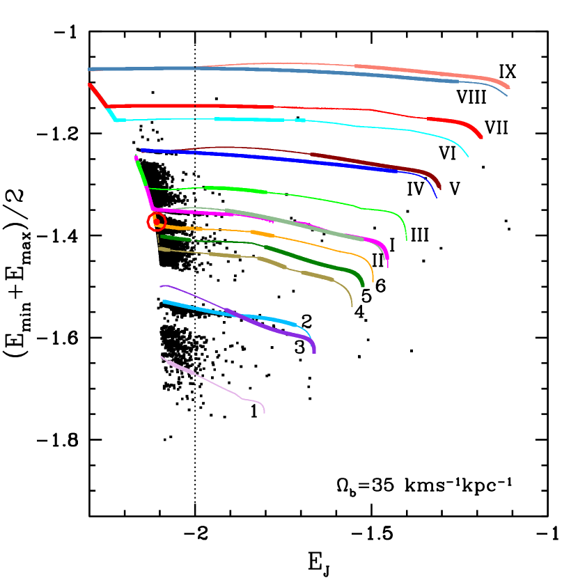
Figure 2: Characteristic energy versus $E_{\rm J}$, in units of 10⁵ km² s^-2 in both axes, showing the fifteen resonant orbital families on the Galactic plane considered in our analysis. The angular velocity of the bar is 35 ${\rm\,km\,s^{-1}{kpc}^{-1}}$ in this figure. The black points correspond to orbits of 2 $\times$ 10⁴ stars taken at random within a 2 kpc-radius solar neighbourhood in Gaia DR2. The thick and thin parts of a curve are respectively the stable and unstable orbital sections of the family. The big red circle with a central dot shows the position of the Sun.

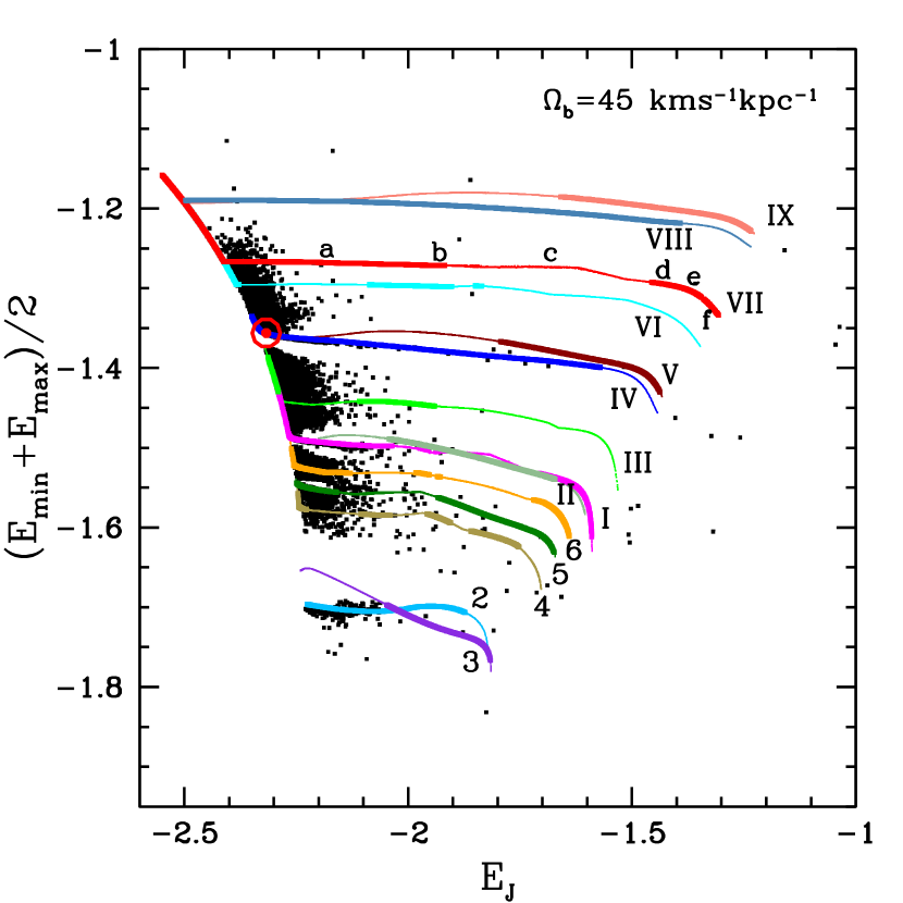
Figure 3: As in Fig. 2, here with an angular velocity of 45 ${\rm\,km\,s^{-1}{kpc}^{-1}}$.

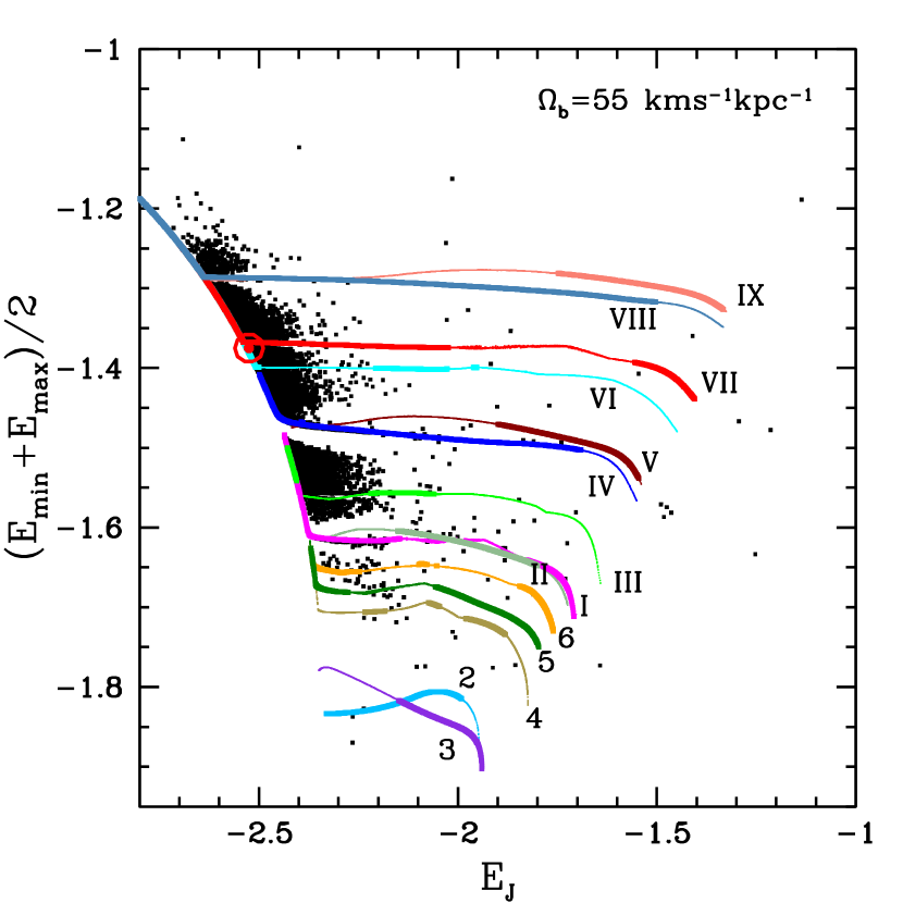
Figure 4: As in Fig. 2, here with an angular velocity of 55 ${\rm\,km\,s^{-1}{kpc}^{-1}}$. Note the downwards shift of the resonant families with respect to their positions in Fig. 2.

Figure 5: Poincaré diagrams at the marked points a – f on the curve of family VII in Fig. 3. These diagrams show a region around the perpendicular crossing of the member periodic orbit in the family with the bar’s long axis. A wide region of islands appears in the marked stable points a,e. These islands do not appear in the unstable point c. In the marked points b,d,f near a stable-unstable transition, the island region is small.

3.2 Periodic Orbits

By taking in Fig. 2 a vertical line (dotted line) at $E_{\rm J}$ = $-2$ $\times$ 10⁵ km² s^-2, the corresponding periodic orbits at the intersections with the resonant families are plotted in Fig. 6. The orbits have the same colour as their parent families. As stated above, the $x^{\prime}$ and $y^{\prime}$ axes on the Galactic plane point along the major and minor axes of the bar, respectively, and corotate with the bar. The Galactic centre is at the origin. The continuous black circle shows the position of the corotation resonance, and the discontinuous circle the outer Lindblad resonance. Fux (2001) shows some periodic orbits obtained with a quadrupole potential bar.

In each panel of Fig. 6 we give the ratio $n/m$, or rotation number (Contopoulos, 2002), of the periodic orbit in the non-inertial frame; $n$ is the number of oscillations in the radial direction when the orbits makes $m$ oscillations around the Galactic centre. The rotation number tends to infinity as we approach corotation resonance. For family 1 this rotation number is denoted with a subindex int, meaning interior to corotation resonance. The given rotation number in a family will change when its orbits change from prograde to retrograde, i.e. when they cross the Galactic centre and the curves in Figs. 2, 3, 4 are extended to the right sides. Families II,V,IX emerge as unstable bifurcations of stable sections of families I,IV,VIII, respectively, and have similar rotation numbers 4/1, 2/1, 1/1. In the following we refer to a family by its number or stating the corresponding $n/m$ resonance.

In particular, the periodic orbits of families 2 and 3 in Fig. 6 are plotted in Fig. 7 showing some zero-velocity curves computed in the Galactic model with $\Omega_{\rm b}$= 35 ${\rm\,km\,s^{-1}{kpc}^{-1}}$. With the notation given in figure 3.14 of Binney & Tremaine (2008), these periodic orbits in families 2,3 lie around Lagrange points $L_{5}$, $L_{1}$, respectively (black dots in Fig. 7); the symmetric orbits around Lagrange points $L_{4}$, $L_{2}$ also belong to these families. In Fig. 7 the red continuous and discontinuous circles, show the corotation resonance and outer Lindblad resonance, respectively.

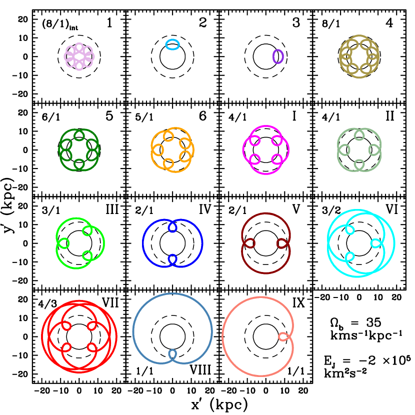
Figure 6: The periodic orbits in each resonant family in Fig. 2 at $E_{\rm J}$ = $-2$, i.e. $E_{\rm J}$ = $-2$ $\times$ 10⁵ km² s^-2 (dotted vertical line in that figure). The colour of an orbit is the same of the family. The $x^{\prime}$ and $y^{\prime}$ axes lie on the Galactic plane, along the major and minor axes of the bar, respectively. The black continuous circle shows the position of the corotation resonance, and the discontinuous circle the outer Lindblad resonance. The rotation number $n/m$ (see main text) of the resonant family is given in the corresponding panel.

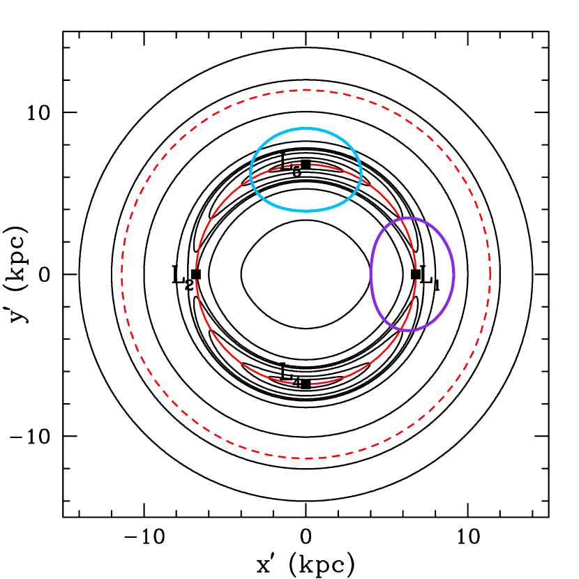
Figure 7: The periodic orbits of families 2 and 3 (blue and purple curves, respectively) in Fig. 6 along with some zero-velocity curves (in black) computed with $\Omega_{\rm b}$= 35 ${\rm\,km\,s^{-1}{kpc}^{-1}}$. These orbits encircle the Lagrange points $L_{5}$, $L_{1}$. The corotation resonance is shown by the red continuous circle; the outer Lindblad resonance lies at the discontinuous red circle. Lagrange points $L_{2}$, $L_{4}$ are also shown.

4 The local U-V velocity field of resonant families crossing the solar neighbourhood

With the stable sections of each resonant family, the next step is to compute the corresponding U-V velocity field of the periodic orbits in each section if they cross the solar neighbourhood. This gives a first estimate of their possible contribution to the observed local U-V field. In Section 5 we will focus in the contributions of trapped orbits around stable periodic orbits.

A solar vicinity on the Galactic plane with radius 500 pc is considered, at the Sun’s galactocentric distance $R_{0}$=8.3 kpc and in the range of values of the angle $\phi_{B}$, between the major axis of the bar and the Sun-Galactic centre line, given in Section 2.2. If a periodic orbit crosses the solar vicinity, it is analysed at close division points, computing at each one the velocity components U,V with respect to the Sun. This is done with the point’s position ($x^{\prime}$,$y^{\prime}$) and velocity ($V_{x^{\prime}}$,$V_{y^{\prime}}$) with respect to the non-inertial reference frame where the bar is at rest, the bar’s angular velocity $\Omega_{\rm b}$, the angle $\phi_{B}$, the LSR velocity $\Theta_{0}$, and the peculiar Solar motion with respect to the LSR, which was taken as $(U,V,W)_{\odot}$=(11.10, 12.24, 7.25)${\rm\,km\,s^{-1}}$ (Schönrich et al., 2010), with $U_{\odot}$ positive towards the Galactic centre, as assumed for U with respect to the Sun. Considering an inertial reference system with origin at the Galactic centre, the $x$-axis pointing to the present position of the Sun, and the $y$-axis pointing in the opposite direction to Galactic rotation, the velocity components U,V of an orbital point with respect to the Sun in terms of the velocity ($V_{x}$,$V_{y}$) in this system are

$$U=-V_{x}+U_{\odot}=-(V_{x^{\prime}}+y^{\prime}\Omega_{\rm b})\cos\phi_{B}-(V_{y^{\prime}}-x^{\prime}\Omega_{\rm b})\sin\phi_{B}+U_{\odot}$$ (7)

$$V=-V_{y}-\Theta_{0}-V_{\odot}=(V_{x^{\prime}}+y^{\prime}\Omega_{\rm b})\sin\phi_{B}-(V_{y^{\prime}}-x^{\prime}\Omega_{\rm b})\cos\phi_{B}-\Theta_{0}-V_{\odot}$$ (8)

As the Sun’s vicinity is located in the first quadrant of the ($x^{\prime}$,$y^{\prime}$) plane, in the resonant families 6,III,VI,IX we take into account their orbital reflections with respect to the $y^{\prime}$-axis, which give periodic orbits belonging to the same families. Also, in family VIII its reflection with respect to the $x^{\prime}$-axis belongs to this family. These reflected orbits exist due to the symmetries of the Galactic potential.

An example of a resonant family which has symmetric orbits with respect to the Galactic centre is given in Fig. 8; it shows the ten analysed solar vicinities and different orbital inner points due to a stable section of family VII, with $\Omega_{\rm b}$=50 ${\rm\,km\,s^{-1}{kpc}^{-1}}$. A particular orbit in the family is plotted. Depending on the solar vicinity, more than one orbital crossing can contribute to the inner points, thus increasing their number in some regions within a given solar vicinity. If this vicinity is empty, there are no crossing points. Figs. 9, 10 show a similar example now with a stable section of family 6, in the case $\Omega_{\rm b}$=40 ${\rm\,km\,s^{-1}{kpc}^{-1}}$. Contributions of the orbital reflection of this family with respect to the $y^{\prime}$-axis are shown in Fig. 10. Two particular orbits in the family are plotted in these figures.

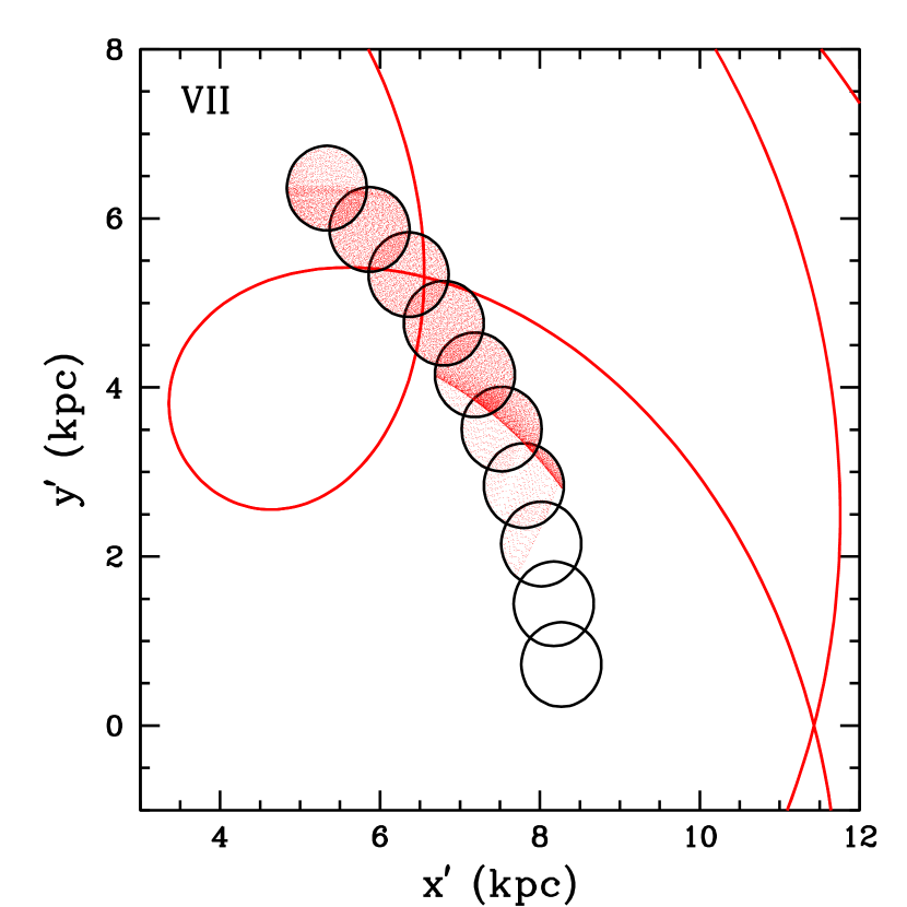
Figure 8: Solar vicinities shown with circles with radius of 500 pc, at different angles $\phi_{B}$, and inner orbital points generated by a stable section of family VII, which is symmetric with respect to the Galactic centre. A particular orbit in the family is plotted. In this example, $\Omega_{\rm b}$=50 ${\rm\,km\,s^{-1}{kpc}^{-1}}$.

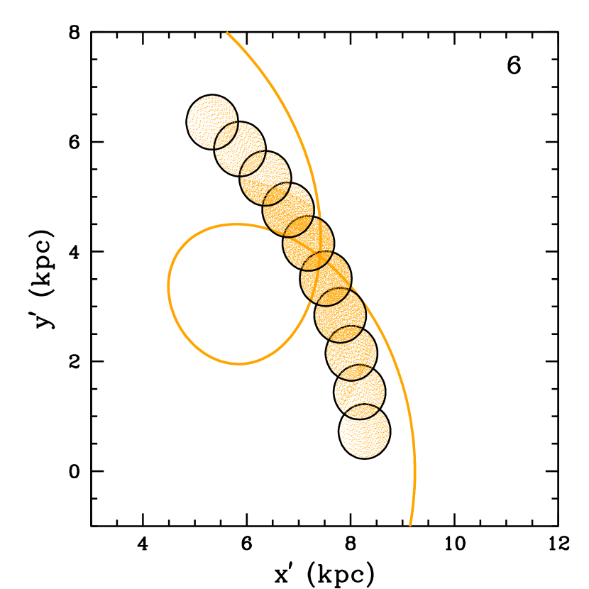
Figure 9: As in Fig. 8, here an example with a stable section of family 6, with $\Omega_{\rm b}$=40 ${\rm\,km\,s^{-1}{kpc}^{-1}}$.

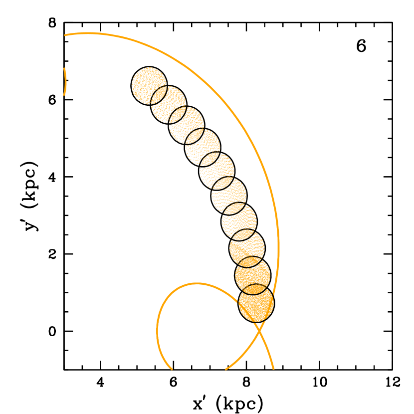
Figure 10: Contributions of family 6 reflected with respect to the $y^{\prime}$-axis, with $\Omega_{\rm b}$=40 ${\rm\,km\,s^{-1}{kpc}^{-1}}$.

The local U-V velocity field with respect to the Sun resulting from stable resonant orbital families must be compared with the observed field. Around zero velocity, this observed U-V field is shown in Fig. 11 taking stars within a 200 pc-radius solar neighbourhood listed in Gaia DR2 (Gaia Collaboration et al., 2018a). The three main branches identified by Skuljan et al. (1999) appear around the centre, moving downwards in the V-axis: the Sirius branch, the Middle branch or Coma Berenices branch, and the Hyades-Pleiades branch. Also, the Hercules branch at V $\approx$ $-50$ ${\rm\,km\,s^{-1}}$ and other structures below this level.

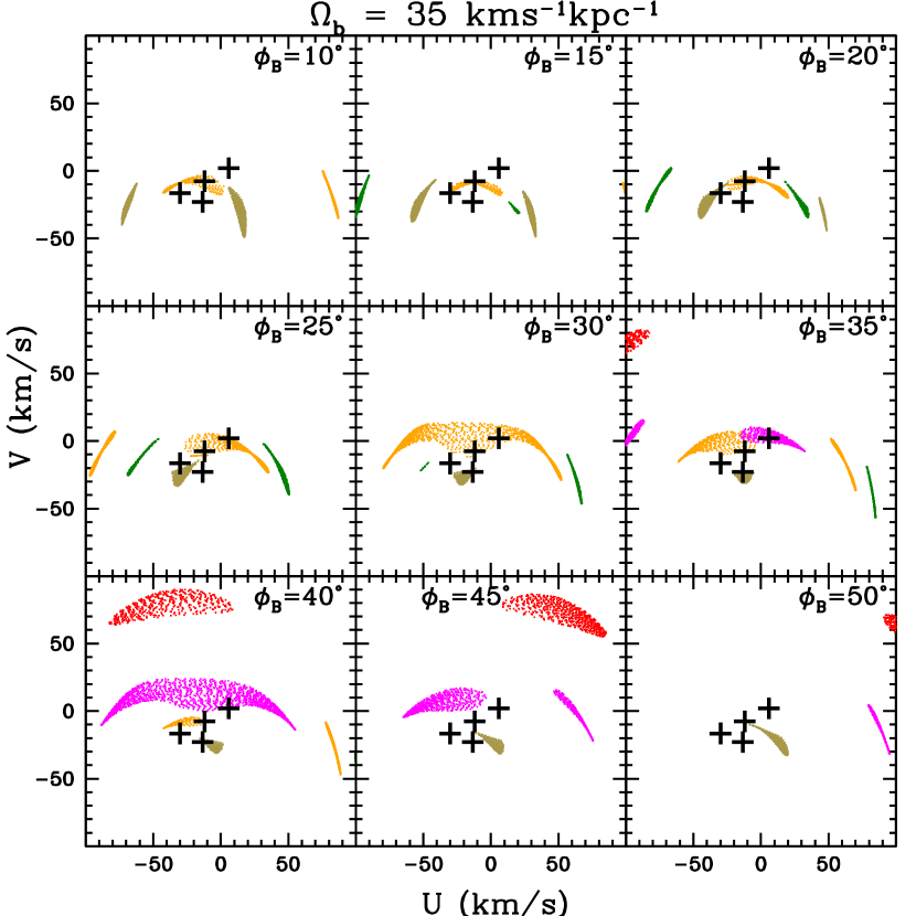
Figure 22: U-V velocities with respect to the Sun of stable sections in resonant families with $\Omega_{\rm b}$=35 ${\rm\,km\,s^{-1}{kpc}^{-1}}$. The family colour is as in Fig. 2. The value of the angle $\phi_{B}$ appears in each panel. The solar vicinity has a radius of 500 pc. The four main density maxima in Fig. 11 are shown with plus signs.

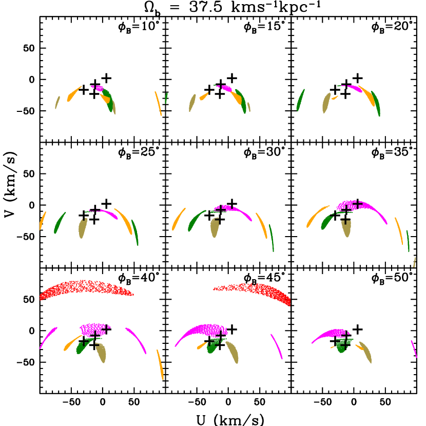
Figure 23: Same as Fig. 22, with $\Omega_{\rm b}$=37.5 ${\rm\,km\,s^{-1}{kpc}^{-1}}$ and different values of the angle $\phi_{B}$.

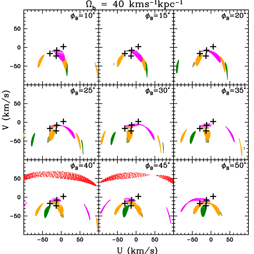
Figure 24: Same as Fig. 22, with $\Omega_{\rm b}$=40 ${\rm\,km\,s^{-1}{kpc}^{-1}}$ and different values of the angle $\phi_{B}$.

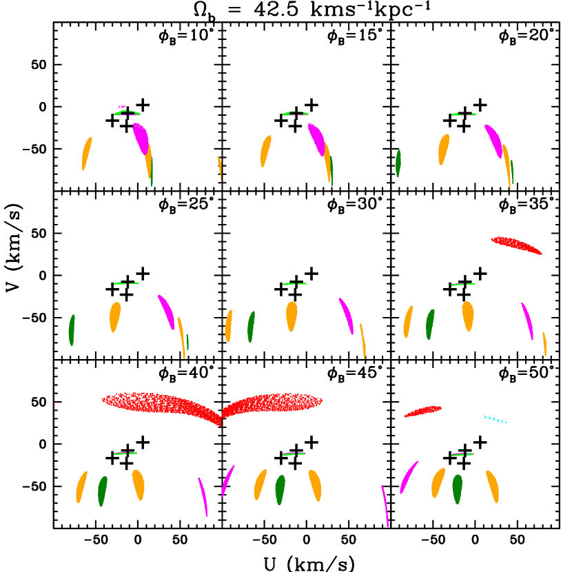
Figure 25: Same as Fig. 22, with $\Omega_{\rm b}$=42.5 ${\rm\,km\,s^{-1}{kpc}^{-1}}$ and different values of the angle $\phi_{B}$.

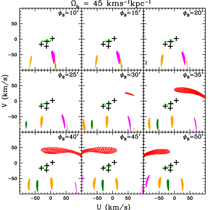
Figure 26: Same as Fig. 22, with $\Omega_{\rm b}$=45 ${\rm\,km\,s^{-1}{kpc}^{-1}}$ and different values of the angle $\phi_{B}$.

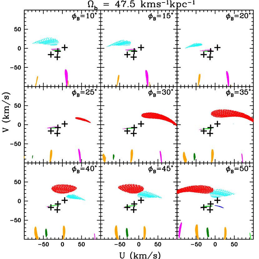
Figure 27: Same as Fig. 22, with $\Omega_{\rm b}$=47.5 ${\rm\,km\,s^{-1}{kpc}^{-1}}$ and different values of the angle $\phi_{B}$.

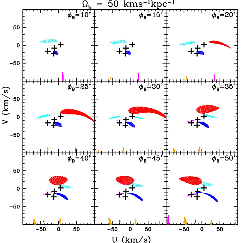
Figure 28: Same as Fig. 22, with $\Omega_{\rm b}$=50 ${\rm\,km\,s^{-1}{kpc}^{-1}}$ and different values of the angle $\phi_{B}$.

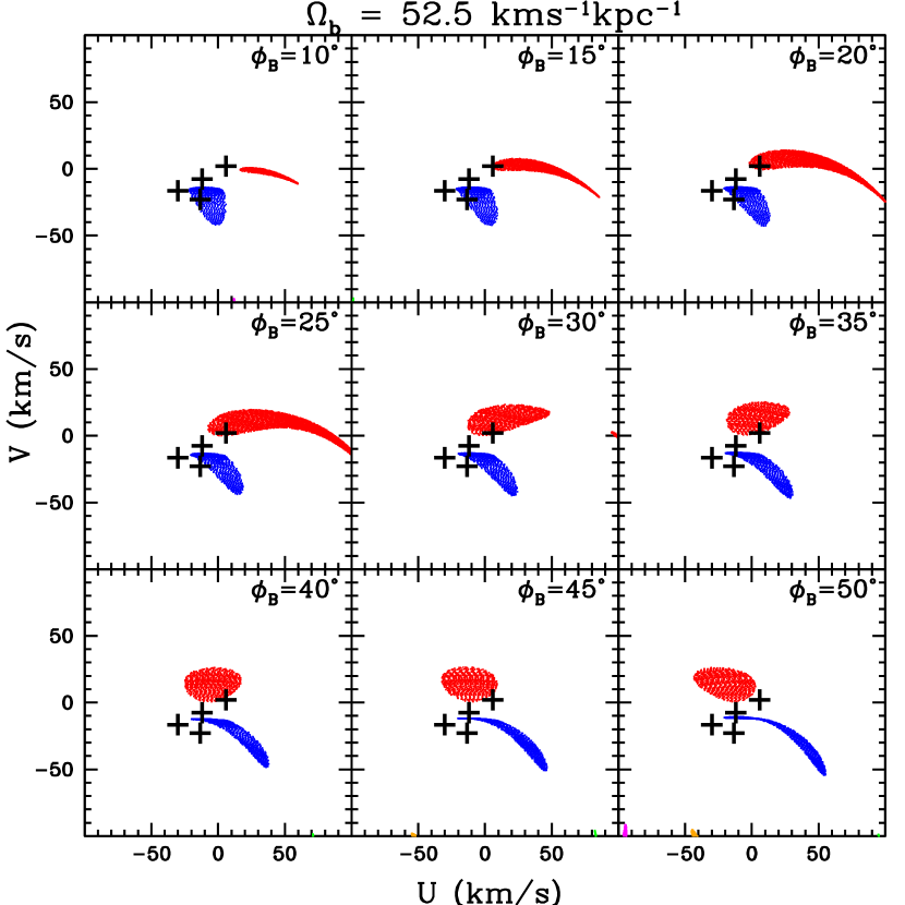
Figure 29: Same as Fig. 22, with $\Omega_{\rm b}$=52.5 ${\rm\,km\,s^{-1}{kpc}^{-1}}$ and different values of the angle $\phi_{B}$.

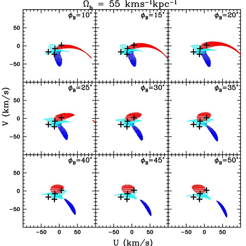
Figure 30: Same as Fig. 22, with $\Omega_{\rm b}$=55 ${\rm\,km\,s^{-1}{kpc}^{-1}}$ and different values of the angle $\phi_{B}$.

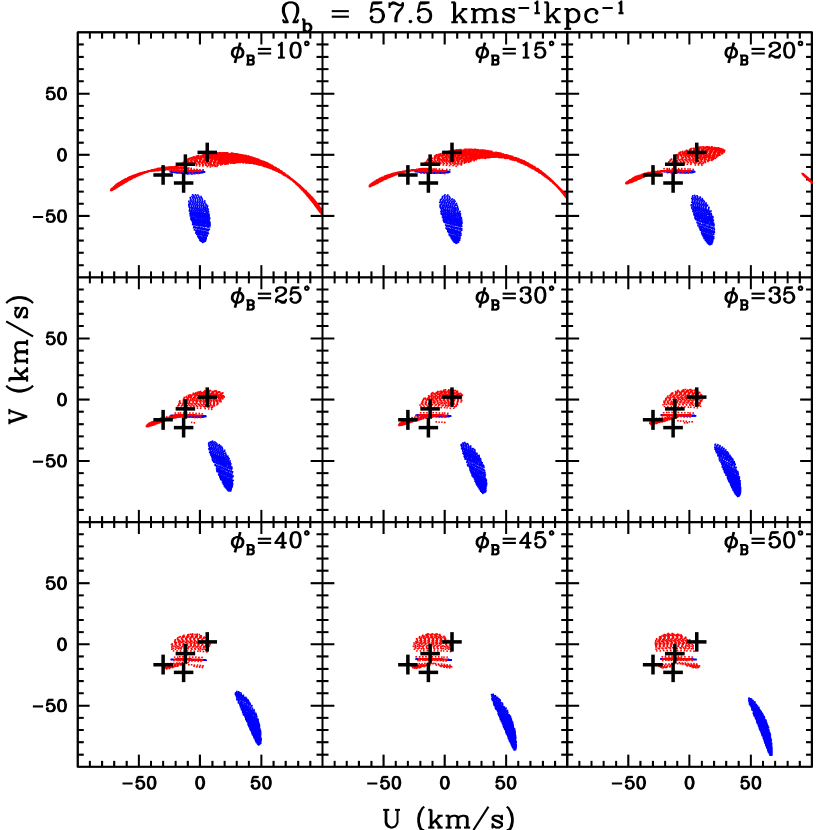
Figure 31: Same as Fig. 22, with $\Omega_{\rm b}$=57.5 ${\rm\,km\,s^{-1}{kpc}^{-1}}$ and different values of the angle $\phi_{B}$.

The resulting U-V contributions of periodic orbits crossing the solar vicinity, in all the stable sections of all the resonant families, are given in Figs. 22 – 31. Each figure has its corresponding value of $\Omega_{\rm b}$, and the angle $\phi_{B}$ appears in each panel. These results were obtained within the 500 pc-radius solar vicinity, as stated above. Each colour gives the family, as in Fig. 2. In these figures we show with plus signs the four main density maxima in Fig. 11. We stress that the agglomerations obtained in these figures represent only contributions to the observed local U-V field that could result from orbital trapping by some resonant families, and do not represent the total field as shown in Fig. 11, which includes possibly trapped and non-trapped stars.

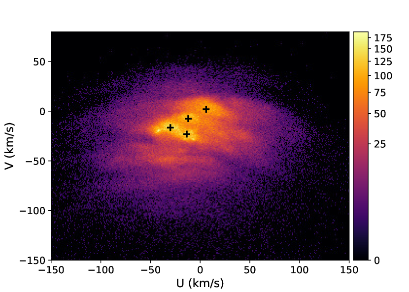
Figure 11: U-V velocities of stars within a 200 pc-radius solar neighbourhood listed in Gaia DR2. The 2D histogram has a size of 1 ${\rm\,km\,s^{-1}}$. The colour scale shows the star number per (${\rm\,km\,s^{-1}}$)². The plus signs show approximately the positions of the four main density maxima.

Some relevant points from these results are the following:

1. With $\Omega_{\rm b}$ $\approx$ 35 – 40 ${\rm\,km\,s^{-1}{kpc}^{-1}}$ the main contributions in U-V velocities due to orbital trapping come from resonant families 4, 5, 6, I. At the other extreme $\Omega_{\rm b}$ $\approx$ 50 – 57.5 ${\rm\,km\,s^{-1}{kpc}^{-1}}$, families IV,VI,VII give the main contributions. This reflects the downwards shift of resonant families shown in Figs. 2, 3, 4: the solar vicinity stays at position $R_{0}$, while resonant families decrease their distance to the Galactic centre as $\Omega_{\rm b}$ increases.

2. Some aglomerations near zero velocity, like those observed in Fig. 11, do not appear with $\Omega_{\rm b}$=42.5, 45, 47.5 ${\rm\,km\,s^{-1}{kpc}^{-1}}$. In our attempt to find a connection between resonant families and the observed U-V field, these values of $\Omega_{\rm b}$ are not considered for further analysis. Thus, the effect of orbital trapping in the local U-V field is expected to be significant only in the low and high values of $\Omega_{\rm b}$.

3. With $\Omega_{\rm b}$=35 – 40 ${\rm\,km\,s^{-1}{kpc}^{-1}}$ there are some contributions of family VII, in red colour, at high values in velocity V with $\phi_{B}$=40^∘, 45^∘. This result is commented in the following section.

4. In the cases with low angular velocity, $\Omega_{\rm b}$=35, 37.5, 40 ${\rm\,km\,s^{-1}{kpc}^{-1}}$, there are some dispersed contributions with V velocities mainly shifted below zero. An extended analysis can be made with $\Omega_{\rm b}$=37.5, 40 ${\rm\,km\,s^{-1}{kpc}^{-1}}$ taking the angles $\phi_{B}$=20^∘ – 40^∘.

5. The cases $\Omega_{\rm b}$=50 – 57.5 ${\rm\,km\,s^{-1}{kpc}^{-1}}$ give contributions of three families IV,VI,VII near zero velocity, whose possible relation with the three main branches identified by Skuljan et al. (1999) can be further analysed.

In the next section we proceed with the analysis of some cases in points (iv) and (v).

5 The local U-V velocity field of trapped orbits

5.1 Trapped Orbits by Periodic Orbits crossing the Solar neighbourhood

The agglomerations in the U-V plane obtained in the last section need a further analysis, taking into account the possible orbital trapping of the corresponding periodic orbits. To represent trapped orbits around stable periodic orbits in a given family a variation of $V_{x^{\prime}}$ was considered from its value $V_{x^{\prime}}$=0 at its perpendicular crossing with the $x^{\prime}$-axis, keeping the original value of the Jacobi constant $E_{\rm J}$. Thus, we move in the vertical direction at the $x^{\prime}$ position of the periodic orbit in an island region of a Poincaré diagram, as in Fig. 5, but staying within this region.

The trapped orbits will be in general 3D orbits, and will have projected tube orbits on the $x^{\prime}$,$y^{\prime}$ plane whose velocity ($V_{x^{\prime}}$,$V_{y^{\prime}}$) can be represented with planar tube orbits around stable resonant families on the Galactic plane (Moreno et al., 2015). The maximum value of $V_{x^{\prime}}$ depends on the given family; we found approximately a representative top limit around 20 ${\rm\,km\,s^{-1}}$ in the families analysed in this section (but in particular for the value of $E_{\rm J}$ in panel a of Fig. 5 this limit is around 40 ${\rm\,km\,s^{-1}}$; thus, the top limit in $V_{x^{\prime}}$ will be changed in some families), and considered the discrete values $V_{x^{\prime}}$=5, 10, 15, 20 ${\rm\,km\,s^{-1}}$ to initiate tube orbits. These orbits were computed up to a total time of 10$t_{\rm per}$, with $t_{\rm per}$ the time in which the associated periodic orbit closes in the non-inertial ($x^{\prime}$,$y^{\prime}$) reference frame. In most cases this total time is around 5 Gyr.

Given $\Omega_{\rm b}$, $\phi_{B}$ and a periodic orbit in a stable section of a resonant family, with its computed tube orbits and their crossings with the corresponding 500 pc-radius solar vicinity, the velocities U,V in Eqs. 7, 8 were obtained at some inner division points. All these points (U,V) in tube orbits are associated with the periodic orbit. All the periodic orbits in a stable section of the resonant family will contribute with a different number of points (U,V). To estimate the relative number contribution of each periodic orbit, a random sample of 5 $\times$ 10⁴ stars in Gaia DR2 (Gaia Collaboration et al., 2018a) within the 500 pc-radius solar vicinity was considered in a characteristic energy versus $E_{\rm J}$ diagram, like in Figs. 2, 3, 4. The number of points in this diagram along a thin band around the stable section of the given resonant family was counted for each $E_{\rm J}$ in the section, taking the lenght $\Delta E_{\rm J}$ as the mean separation of periodic orbits in our computations. These numbers give an estimate of the relative number of trapped orbits along the stable section of the family, and they were employed to rescale the numbers of computed points (U,V) in tube orbits at each $E_{\rm J}$.

We followed this procedure to analize the cases with $\Omega_{\rm b}$=37.5, 40 ${\rm\,km\,s^{-1}{kpc}^{-1}}$ in Figs. 23, 24, taking the angles $\phi_{B}$=20^∘ – 35^∘ in the first case, and $\phi_{B}$=25^∘ – 40^∘ in the second. Also the cases $\Omega_{\rm b}$=55, 57.5 ${\rm\,km\,s^{-1}{kpc}^{-1}}$ in Figs. 30, 31 with $\phi_{B}$=10^∘ – 25^∘. The results are shown in Figs. 12–15, taking points (U,V) only within a 200 pc-radius solar vicinity, in order to compare with Fig. 11.

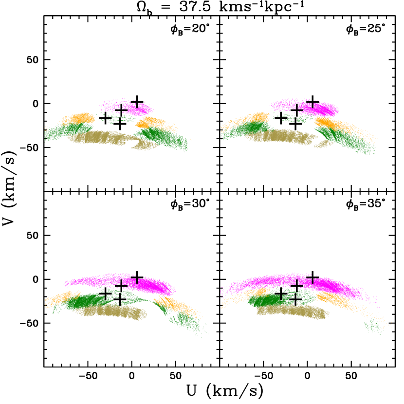
Figure 12: Resonant bands produced by families 4, 5, 6, I, taking tube orbits around periodic orbits in stable family sections with $\Omega_{\rm b}$=37.5 ${\rm\,km\,s^{-1}{kpc}^{-1}}$. See the family colour in Fig. 2. The value of the angle $\phi_{B}$ appears in each panel. In order to compare with Fig. 11 here the solar vicinity has a radius of 200 pc. We show with plus signs the four main density maxima in Fig. 11.

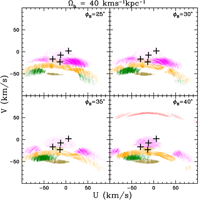
Figure 13: Same as Fig. 13, here with $\Omega_{\rm b}$=40 ${\rm\,km\,s^{-1}{kpc}^{-1}}$. Note the Hercules branch at V=$-50$ ${\rm\,km\,s^{-1}}$ produced by family 4, or resonance 8/1.

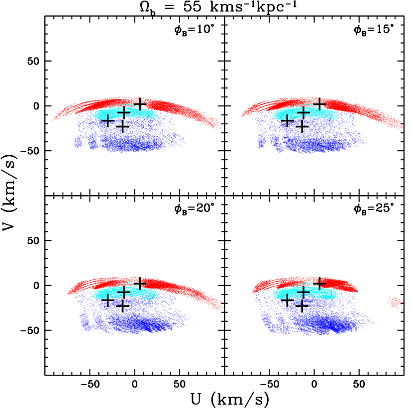
Figure 14: As in Fig. 13, with $\Omega_{\rm b}$=55 ${\rm\,km\,s^{-1}{kpc}^{-1}}$; here the resonant bands are generated by families IV,VI,VII.

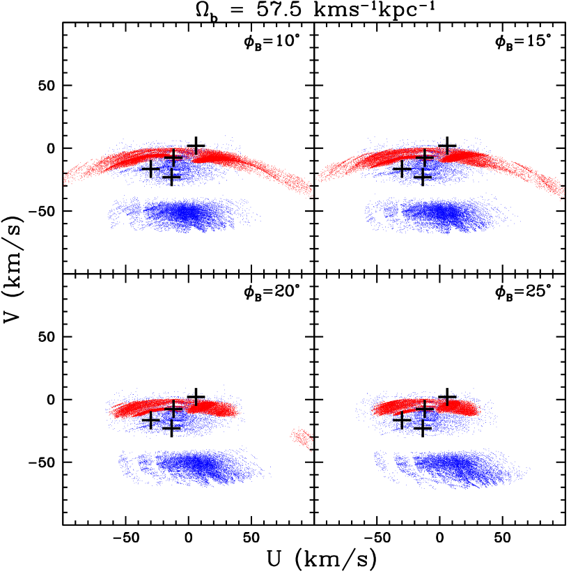
Figure 15: As in Fig. 13, with $\Omega_{\rm b}$=57.5 ${\rm\,km\,s^{-1}{kpc}^{-1}}$; here the resonant bands are generated by families IV and VII.

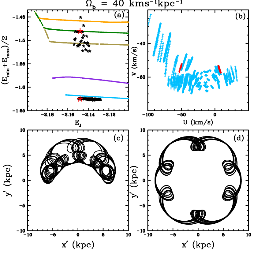
Figure 16: Orbits constructed from family 2 can give points U,V around the Hercules stream. Here $\Omega_{\rm b}$=40 ${\rm\,km\,s^{-1}{kpc}^{-1}}$, $\phi_{B}$=40^∘ are considered, with a 500 pc-radius solar vicinity. Panel (a) shows a region of the characteristic energy vs $E_{J}$ diagram with families 2,3,4,5,6. The black starred points near the blue curve of family 2 represent orbits inside the island regions around some of its periodic orbits but close to their boundaries. The black points lying in the region of families 4,5,6 (brown, green, and orange curves) represent orbits taken outside the island regions of family 2. The red points are two particular orbits. Panel (b) shows the resulting U-V plane due to the starred points in panel (a). The (U,V) points distribute around the Hercules stream. Panels (c) and (d) show the orbits corresponding to the lower and upper red points in panel (a).

In each case shown in these figures the resonant families generate some bands of points U,V. Up to four bands can appear in the low values $\Omega_{\rm b}$=37.5, 40 ${\rm\,km\,s^{-1}{kpc}^{-1}}$, resulting from families 4, 5, 6, I. Three main bands are obtained with families IV,VI,VII in the other extreme $\Omega_{\rm b}$=55, 57.5 ${\rm\,km\,s^{-1}{kpc}^{-1}}$. The inclination of these bands with respect to the U-axis is slightly greater with low $\Omega_{\rm b}$, and their width is similar to the width of the three main branches in Fig. 11, the Sirius, Coma Berenices, and Hyades-Pleiades branches.

The cases with $\Omega_{\rm b}$=40, 55, 57.5 ${\rm\,km\,s^{-1}{kpc}^{-1}}$ give structures around level V=$-50$ ${\rm\,km\,s^{-1}}$, close to the Hercules branch. The case $\Omega_{\rm b}$=40 ${\rm\,km\,s^{-1}{kpc}^{-1}}$ approximates better the agglomeration of bands around this V-level shown in the Gaia data in Fig. 11. In this case the Hercules branch is produced by family 4 (brown colour), or resonance 8/1 outside corotation, and the near families 5 (dark green colour) and 6 (orange colour), i.e. respectively resonances 6/1 and 5/1, contribute above family 4.

Another interesting structure which can be approximated with $\Omega_{\rm b}$=40 ${\rm\,km\,s^{-1}{kpc}^{-1}}$, and specially with $\phi_{B}$=40^∘, is the newly detected low-density arch at V $\simeq$ 40 ${\rm\,km\,s^{-1}}$, which has been commented by Gaia Collaboration et al. (2018b) in the U-V plane of their figure 22, and appears in our similar Fig. 11. In our results this arch is approximated by orbital trapping due to family VII, i.e. the resonance 4/3.

In the dynamical model of Pérez-Villegas et al. (2017) with $\Omega_{\rm b}$=39 ${\rm\,km\,s^{-1}{kpc}^{-1}}$ the Hercules stream is approximated by stars orbiting the Lagrange points $L_{4}$, $L_{5}$, thus associated with our family 2 (see Fig. 6), or circulating between both points. Points U,V due to family 2 do not appear in Figs. 12, 13 because for the computations in this section, which refer to orbital trapping due to periodic orbits crossing the solar neighbourhood, we did not find periodic orbits of family 2 satisfying this condition. In the next section we consider the missing contribution in the solar vicinity of tube orbits around periodic orbits in family 2, and other families, which are external to this vicinity.

To show how orbits constructed from family 2 can give points U,V around the Hercules stream, a similar computation to that made by Pérez-Villegas et al. (2017) is shown in Fig. 16, using $\Omega_{\rm b}$=40 ${\rm\,km\,s^{-1}{kpc}^{-1}}$ with $\phi_{B}$=40^∘. Panel (a) in this figure is the characteristic energy vs $E_{J}$ diagram showing only a region with families 2,3,4,5,6. The black starred points near the blue curve of family 2 represent orbits inside the island regions around some of its periodic orbits but close to their boundaries. The black points lying in the region of families 4,5,6 (brown, green, and orange curves) represent orbits taken outside the island regions of family 2, i.e. they are not necessarily circulating between the Lagrange points $L_{4}$, $L_{5}$, but have jumped to another region. The red points are two particular orbits in these two sets. Panel (b) shows the resulting U-V plane due to all black and red points in panel (a), taking a 500 pc-radius solar vicinity. The (U,V) points distribute around the Hercules stream. Thus, points in this region can be obtained by orbital trapping in the corotation resonance and close resonant families. Panels (c) and (d) show, respectively, the orbits corresponding to the lower and upper red points in panel (a). An important continuation of this Fig. 16 is presented in the following section, taking values of $E_{J}$ greater than those considered in panel (a).

5.2 Trapped Orbits by Periodic Orbits not crossing the Solar neighbourhood

Now we take into account orbital trapping by stable sections of resonant families whose periodic orbits do not cross the given solar vicinity. In these cases, the amplitude of the corresponding tube orbits around periodic orbits is increased until they cross the solar vicinity, and their velocity field (U,V) is computed following the procedure given in Section 5.1. In the present section only two cases are considered of those analysed in Section 5.1: $\Omega_{\rm b}$=40 ${\rm\,km\,s^{-1}{kpc}^{-1}}$ with $\phi_{B}$=40^∘ from Fig. 13, and $\Omega_{\rm b}$=55 ${\rm\,km\,s^{-1}{kpc}^{-1}}$ with $\phi_{B}$=10^∘ from Fig. 14.

With $\Omega_{\rm b}$=40 ${\rm\,km\,s^{-1}{kpc}^{-1}}$ the additional resonant families which are analysed are 2,3,IV,V,VI,VIII; with $\Omega_{\rm b}$=55 ${\rm\,km\,s^{-1}{kpc}^{-1}}$ the additional families are 2,3,V,VIII,IX. The contributions of all these families are plotted only in the interval [-100,100] ${\rm\,km\,s^{-1}}$ of velocities U,V, as in figures of the preceeding section.

In Fig. 17 we show the complete case $\Omega_{\rm b}$=40 ${\rm\,km\,s^{-1}{kpc}^{-1}}$, $\phi_{B}$=40^∘, adding the contributions obtained in this section to those shown in Fig. 13. The few steel blue (see family colours in Fig. 6) points in the arch at V $\simeq$ 80 ${\rm\,km\,s^{-1}}$ correspond to family VIII, resonance 1/1. Points like these are not detected in Fig. 11. The blue points in the arch between 20 – 40 ${\rm\,km\,s^{-1}}$ in velocity V correspond to family IV, resonance 2/1. Points like these do appear in Fig. 11. The sky blue points in the inclined structure below the Hercules branch correspond to family 2, corotation resonance. This structure is detected in Fig. 11.

In Fig. 18 the inclined structure due to family 2 is further analysed. Panel (a) is a continuation of panel (a) in Fig. 16, here taking greater values of $E_{J}$. The dense black points close to the blue curve of family 2 represent tube orbits trapped by periodic orbits in this family, with their amplitudes taken such that they may cross the solar vicinity. The red point is a particular orbit. Panel (b) shows the velocity points (U,V) generated by all these orbits within the solar vicinity; the red points correspond to the red point in panel (a). Thus, these orbits generate the inclined structure in Fig. 17. Panel (c) shows the stable periodic orbit in family 2 at the value $E_{J}$ of the red point in panel (a), and panel (d) is the tube orbit of this red point.

In Fig. 19 we show the complete case $\Omega_{\rm b}$=55 ${\rm\,km\,s^{-1}{kpc}^{-1}}$, $\phi_{B}$=10^∘, adding the contributions obtained in this section to those shown in Fig. 14. Family VIII contributes with the arch at 30 – 40 ${\rm\,km\,s^{-1}}$ in velocity V, and family 2 gives the points around V $\simeq$ $-90$ ${\rm\,km\,s^{-1}}$. In this case the inclined feature in Fig. 17 is not obtained.

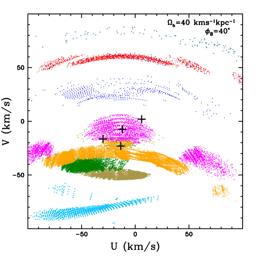
Figure 17: The complete case $\Omega_{\rm b}$=40 ${\rm\,km\,s^{-1}{kpc}^{-1}}$, $\phi_{B}$=40^∘, adding the contributions obtained in Section 5.2 to those shown in Fig. 13. The few steel blue (see family colours in Fig. 6) points in the arch at V $\simeq$ 80 ${\rm\,km\,s^{-1}}$ correspond to family VIII, resonance 1/1. Points like these are not detected in Fig. 11. The blue points in the arch between 20 – 40 ${\rm\,km\,s^{-1}}$ in velocity V correspond to family IV, resonance 2/1. Points like these do appear in Fig. 11. The sky blue points in the inclined structure below the Hercules branch correspond to family 2, corotation resonance. This structure is detected in Fig. 11.

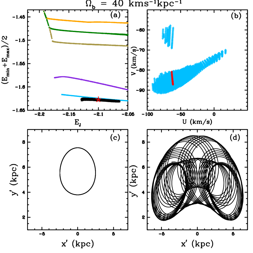
Figure 18: Analysis of the inclined structure due to family 2 in Fig. 17. Panel (a) is a continuation of panel (a) in Fig. 16, here taking greater values of $E_{J}$. The dense black points close to the blue curve of family 2 represent tube orbits trapped by periodic orbits in this family, with their amplitudes taken such that they may cross the solar vicinity. The red point is a particular orbit. Panel (b) shows the velocity points (U,V) generated by all these orbits within the solar vicinity; the red points correspond to the red point in panel (a). Thus, these orbits generate the inclined structure in Fig. 17. Panel (c) shows the stable periodic orbit in family 2 at the value $E_{J}$ of the red point in panel (a), and panel (d) is the tube orbit of this red point.

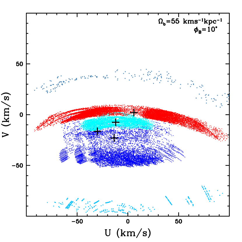
Figure 19: The complete case $\Omega_{\rm b}$=55 ${\rm\,km\,s^{-1}{kpc}^{-1}}$, $\phi_{B}$=10^∘, adding the contributions obtained in Section 5.2 to those shown in Fig. 14. Family VIII contributes with the arch at 30 – 40 ${\rm\,km\,s^{-1}}$ in velocity V, and family 2 gives the points around V $\simeq$ $-90$ ${\rm\,km\,s^{-1}}$.

With these results, our best approximation to the local velocity field by orbital trapping is $\Omega_{\rm b}$=40 ${\rm\,km\,s^{-1}{kpc}^{-1}}$ with $\phi_{B}$=40^∘. Based on data taken by APOGEE-2S, the analysis given by Hunt et al. (2018) favor a fast bar with $\Omega_{\rm b}$=48.6 ${\rm\,km\,s^{-1}{kpc}^{-1}}$. More recent studies support a slow bar (Monari et al., 2019a, b; Sanders et al., 2019; Clarke et al., 2019; Bovy et al., 2019) with $\Omega_{\rm b}$ around 40 ${\rm\,km\,s^{-1}{kpc}^{-1}}$. In particular, Monari et al. (2019a) show that a bar with $\Omega_{\rm b}$=39 ${\rm\,km\,s^{-1}{kpc}^{-1}}$ creates most of the observed structures in local action space which are related to resonances generated by the bar. We identify some bands of points U,V in Fig. 17 with resonance lines in their figure 4: our families I and 5 are related with their resonances 4/1 and 6/1, respectively; the band of family 6 is the resonance 5/1 not shown in their figure 4; the resonance 3/1, associated to family III, is slightly appearing with $\Omega_{\rm b}$=40 ${\rm\,km\,s^{-1}{kpc}^{-1}}$, $\phi_{B}$=10^∘,15^∘,20^∘ in Fig. 24, but is strong with $\Omega_{\rm b}$=42.5, 45 ${\rm\,km\,s^{-1}{kpc}^{-1}}$ in Figs. 25, 26. The low-density arch at V $\simeq$ 40 ${\rm\,km\,s^{-1}}$ in Fig. 11 appears to be related with the outer Lindblad resonance 2/1 in figure 4 of Monari et al. (2019a), and is obtained by orbital simulations with a slow bar given by Hunt & Bovy (2018). With our results in Fig. 17 this arch can be approximated with family VII, i.e. resonance 4/3, but also the wide arch due to resonance 2/1 (family IV) is close to this structure.

Our analysis has considered only the effects of bar resonances in the U-V local velocity field, but there are other studies which include also a spiral pattern. With test particle simulations, Chakrabarty (2007) concludes that a bar, with an angular velocity of $\Omega_{\rm b}$=57.4 ${\rm\,km\,s^{-1}{kpc}^{-1}}$, and a 4-armed spiral can approximate the main concentrations in the U-V plane. A similar conclusion is reached by Michtchenko et al. (2018a, b), with a 4-arms spiral and a bar with low mass $10^{9}M_{\odot}$, both rotating with an angular velocity 28.5 ${\rm\,km\,s^{-1}{kpc}^{-1}}$. Antoja et al. (2011), also with test particle simulations, including a bar and a 2-armed spiral, obtain concentrations similar to the observed, but the appearence of these features depends on the integration time. Regarding the Hercules branch, Michtchenko et al. (2018a, b) find that this feature emerges in the 8/1 resonance due to the spiral arms, and the other observed main concentrations are related with the corotation zone of these arms. This result with their low mass $10^{9}M_{\odot}$ of the bar, is different from the one we find here with a bar of $10^{10}M_{\odot}$ and no spiral arms: the Hercules branch is mainly generated by the 8/1 resonance of this bar. The model of Michtchenko et al. (2018a, b) is supported by a recent study of Barros et al. (2020), who show that with that model the local structures in the U-V velocity distribution are well reproduced. Thus, it would be interesting to pursue an analysis to see under what conditions the approximate matches we have obtained with a bar of $10^{10}M_{\odot}$ can be sustained including a spiral pattern, and how well resonant families due to the bar survive.

5.3 Trapped Orbits in the Galactic Halo

We have commented the results obtained around the four main branches in the U,V plane, but it is interesting to give also the predicted contributions of orbital trapping in other regions, considering stellar motions representing the Galactic halo. In this part we take our best case $\Omega_{\rm b}$=40 ${\rm\,km\,s^{-1}{kpc}^{-1}}$, $\phi_{B}$=40^∘. Fig. 20 shows the expected contributions of stable periodic orbits in all the analysed families, taking a 500 pc-radius solar vicinity. This figure is an extension of the lower left panel in Fig. 24. As stated in Section 3.1, only prograde orbits are considered in our analysis, thus contributions below V $\approx$ $-260$ ${\rm\,km\,s^{-1}}$ are missing in this figure. No support by orbital trapping is obtained around (U,V)=(0,$-100$) ${\rm\,km\,s^{-1}}$, the region of the Arcturus stream (Eggen, 1971; Williams et al., 2009; Kushniruk & Bensby, 2019). Particular strong contributions of families 6,II,V appear in the halo region, around U=200 ${\rm\,km\,s^{-1}}$. These structures seem to be related with star groups G18-39 and G21-22 in the Galactic halo identified by Silva et al. (2012) and plotted in the U-V plane in their figure 7. These two groups have star members mostly in retrograde orbits. Thus, in order to see if there is a possible relation between results in Fig. 20 with these groups, we have extended in particular the family V towards the retrograde region, and have computed tube orbits which can reach the solar vicinity. Fig. 21 shows this extended contribution of family V, along with those of families 6 and II. The updated points of groups G18-39 and G21-22 are shown with red and green colours, as in figure 7 of Silva et al. (2012). A possible relation with these groups is obatined only in the right side of the figure. Further analysis would be needed to see if orbital trapping of both groups might be an alternate explanation to that proposed by Silva et al. (2012), due to the accretion of a dwarf galaxy.

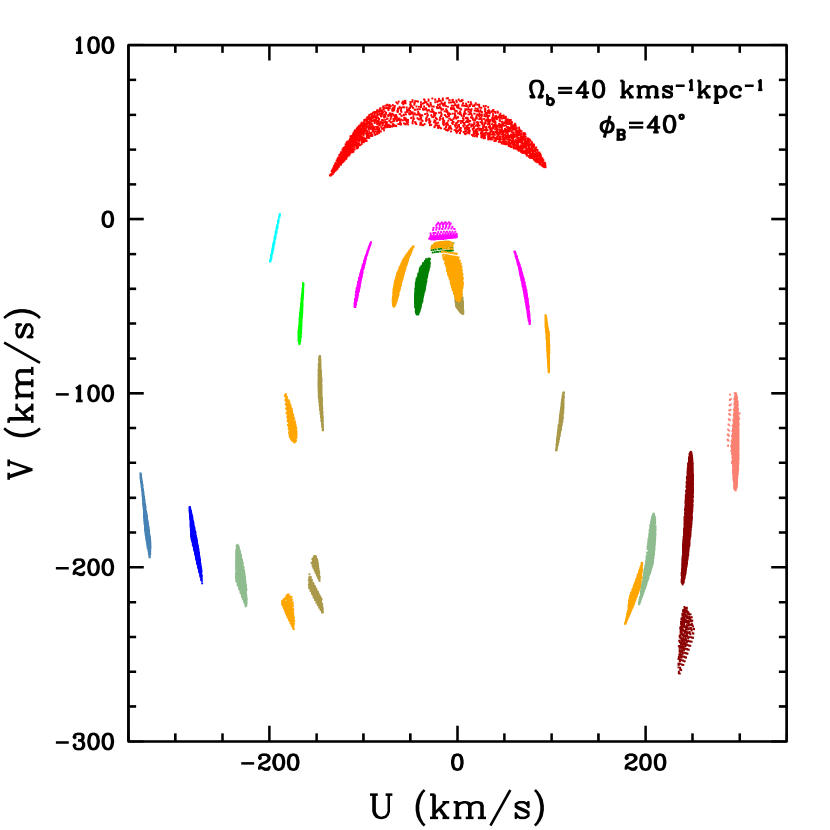
Figure 20: Contributions of periodic orbits crossing the 500 pc-radius solar vicinity in all the analysed resonant families, with $\Omega_{\rm b}$=40 ${\rm\,km\,s^{-1}{kpc}^{-1}}$, $\phi_{B}$=40^∘.

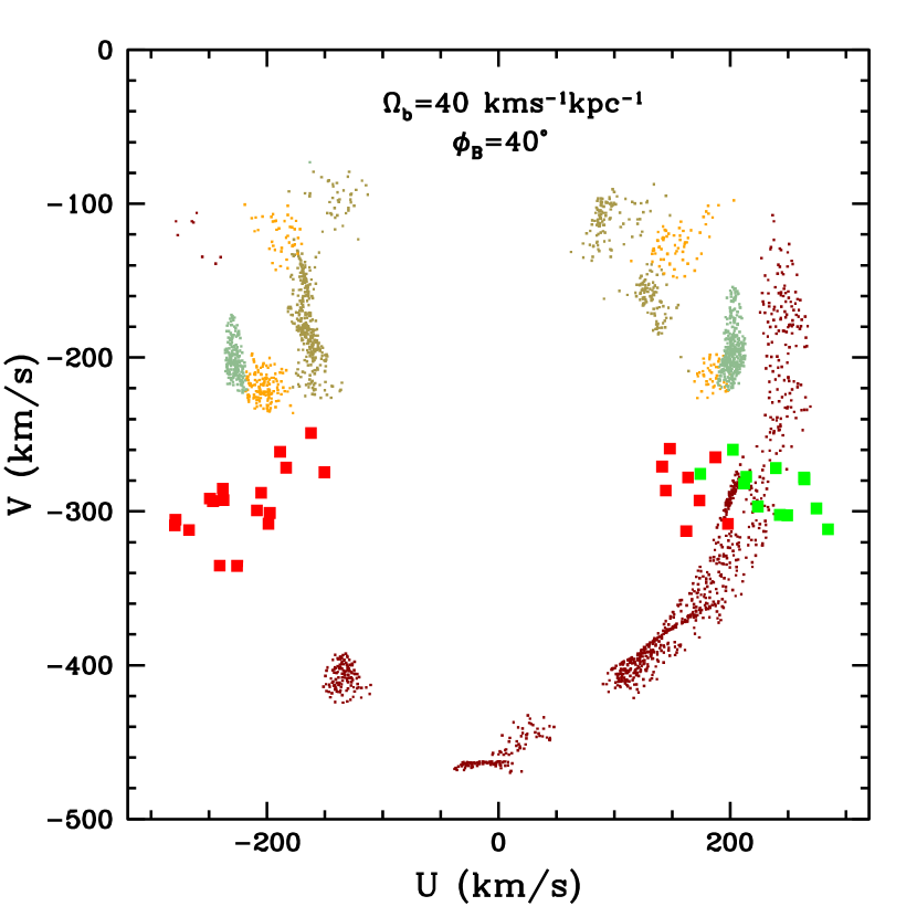
Figure 21: Contributions of trapped orbits in regions of families 6,II,V in Fig. 20, with family V extended towards the retrograde region. The points of groups G18-39 and G21-22 in the Galactic halo are shown with red and green colours.

6 Conclusions

Employing a Galactic potential including a bar, we have analysed the local U-V velocity field and looked for possible effects of orbital trapping by bar resonances on the Galactic plane. Fifteen resonant families have been computed considering ten values of the bar’s angular velocity, $\Omega_{\rm b}$, between 35 and 57.5 ${\rm\,km\,s^{-1}{kpc}^{-1}}$, taking in each one ten values of the angle between the bar’s major axis and the Sun-Galactic centre line, $\phi_{B}$, in the range 5^∘ – 50^∘. In each combination ($\Omega_{\rm b}$,$\phi_{B}$) of these two parameters, we consider the orbital crossings within a 500 pc-radius solar vicinity of the stable periodic orbits in each resonant family. The resulting U-V field of these stable orbits in each family gives a first estimate of their possible contribution to the observed U-V field due to orbital trapping. Considering only combinations ($\Omega_{\rm b}$,$\phi_{B}$) whose resulting contributions may be similar to the observed U-V field, with its four main branches: Sirius, Coma Berenices, Hyades-Pleiades, and Hercules, we find that the cases which may give some similarity with these observed features are in the low range $\Omega_{\rm b}$=37.5, 40 ${\rm\,km\,s^{-1}{kpc}^{-1}}$, and in the high range $\Omega_{\rm b}$=55, 57.5 ${\rm\,km\,s^{-1}{kpc}^{-1}}$. In these cases, and for each stable periodic orbit in a family crossing the solar vicinity, some representative tube orbits on the Galactic plane have been computed, keeping their velocity (U,V) at some orbital division points if they cross this vicinity. These velocity points will represent 3D stellar orbits trapped by resonant families on the Galactic plane. The resulting structures in the local U-V plane form resonant bands appearing at various levels in velocity V. We find that cases $\Omega_{\rm b}$=40, 55 ${\rm\,km\,s^{-1}{kpc}^{-1}}$ show the greatest similarity with the observed main branches. Regarding particular features in the local U-V plane, we find that with the slow bar velocity $\Omega_{\rm b}$=40 ${\rm\,km\,s^{-1}{kpc}^{-1}}$ the Hercules branch at V=$-50$ ${\rm\,km\,s^{-1}}$ can be obtained by orbital trapping in family 4, i.e. the resonance 8/1 outside corotation, and the close features produced by resonances 5/1 and 6/1. Also with this velocity and with an angle $\phi_{B}$=40^∘, orbital trapping is able to reproduce the newly detected low-density arch at V $\simeq$ 40 ${\rm\,km\,s^{-1}}$ shown by Gaia DR2 data. Adding to these results the orbital trapping contributions of resonant families whose periodic orbits do not cross the given solar vicinity, we have found the inclined structure below the Hercules branch (Fig. 17), which is also observed in the Gaia DR2 data. This structure is produced by tube orbits around Lagrange point $L_{5}$. Another obtained feature is an arch between 20 – 40 ${\rm\,km\,s^{-1}}$ in velocity V, due to family IV, i.e. resonance 2/1. Thus, our best approximation to the local velocity field by orbital trapping is $\Omega_{\rm b}$=40 ${\rm\,km\,s^{-1}{kpc}^{-1}}$ with $\phi_{B}$=40^∘. With this solution, we give some predicted contributions due to orbital trapping in regions of the U-V plane corresponding to the Galactic halo, which could help to further restrict the value of the angular velocity of the Galactic bar. In these regions, no support by orbital trapping is found for the Arcturus stream at V $\approx$ $-100$ ${\rm\,km\,s^{-1}}$. Some support is found for the halo moving groups G18-39 and G21-22 at U $\approx$ 200 ${\rm\,km\,s^{-1}}$. Considering the results of our analysis, compared with existing studies which employ a bar with a low mass and include a spiral pattern, it would be interesting to reconsider the effect of orbital trapping taking into account, in addition to a bar of higher mass, the effect of the spiral arms. It is important to see in this case under what conditions the approximate matches that we have obtained can be sustained including the spiral arms, and how well resonant families due to the bar survive.

Data Availability

Data available on request.

Appendix A U-V contributions of stable periodic orbits in all the resonant families

Here we show the resulting U-V contributions of periodic orbits crossing a 500 pc-radius solar vicinity, in all the stable sections of all the resonant families. Each figure has its corresponding value of $\Omega_{\rm b}$, and the angle $\phi_{B}$ appears in each panel. The four main density maxima in Fig. 11 are shown with plus signs.

References

- Allen & Santillán (1991) Allen C.,Santillán A., 1991, Rev. Mex. Astron. Astrofis., 22, 255
- Antoja et al. (2008) Antoja T., Figueras F., Fernández D., Torra J., 2008, A&A, 490, 135
- Antoja et al. (2009) Antoja T., Valenzuela O., Pichardo B., Moreno E., Figueras F., Fernández D., 2009, ApJ, 700, L78
- Antoja et al. (2010) Antoja T., Valenzuela O., Figueras F., Pichardo B., Moreno E., 2010, Highlights of Astronomy, 15, 192
- Antoja et al. (2011) Antoja T., Figueras F., Romero-Gómez M., Pichardo B., Valenzuela O., Moreno E., 2011, MNRAS, 418, 1423
- Antoja et al. (2014) Antoja T. et al., 2014, A&A, 563, A60
- Asiain et al. (1999) Asiain R., Figueras F., Torra J., Chen B., 1999, A&A, 341, 427
- Babusiaux & Gilmore (2005) Babusiaux C., Gilmore G., 2005, MNRAS, 358, 1309
- Barros et al. (2020) Barros D. A., Pérez-Villegas A., Lépine J. R. D., Michtchenko T. A., Vieira R. S. S., 2020, ApJ, 888, 75
- Benjamin et al. (2005) Benjamin R. A. et al., 2005, ApJ, 630, L149
- Bensby et al. (2007) Bensby T., Oey M. S., Feltzing S., Gustafsson B., 2007, ApJ, 655, L89
- Binney & Tremaine (2008) Binney J., Tremaine S., 2008, Galactic Dynamics 2nd Ed. (Princeton: Princeton University Press)
- Bissantz et al. (2003) Bissantz N., Englmaier P., Gerhard O., 2003, MNRAS, 340, 949
- Bland-Hawthorn & Gerhard (2016) Bland-Hawthorn J., Gerhard O., 2016, ARA&A, 54, 529
- Bobylev & Bajkova (2016) Bobylev V. V., Bajkova A. T., 2016, Astronomy Letters, 42, 228
- Bovy et al. (2019) Bovy J., Leung H. W., Hunt J. A. S., Mackereth J. T, García-Hernández D. A, Roman-Lopes A., 2019, MNRAS, 490, 4740
- Brunthaler et al. (2011) Brunthaler A. et al., 2011, Astronomische Nachrichten, 332, 461
- Chakrabarty (2007) Chakrabarty D., 2007, A&A, 467, 145
- Chereul et al. (1999) Chereul E., Crézé M., Bienaymé O., 1999, A&AS, 135, 5
- Clarke et al. (2019) Clarke J. P., Wegg C., Gerhard O., Smith L. C, Lucas P. W., Wylie S. M., 2019, MNRAS, 489, 3519
- Contopoulos (2002) Contopoulos G., 2002, Order and Chaos in Dynamical Astronomy (Berlin: Springer-Verlag)
- Dehnen (1998) Dehnen W., 1998, AJ, 115, 2384
- Dehnen (1999) Dehnen W., 1999, ApJ, 524, L35
- Dehnen (2000) Dehnen W., 2000, AJ, 119, 800
- De Simone et al. (2004) De Simone R., Wu X., Tremaine S., 2004, MNRAS, 350, 627
- Eggen (1971) Eggen O. J., 1971, PASP, 83, 271
- Englmaier & Gerhard (1999) Englmaier P., Gerhard O., 1999, MNRAS, 304, 512
- Famaey et al. (2005) Famaey B., Jorissen A., Luri X., Mayor M., Udry S., Dejonghe H., Turon C., 2005, A&A, 430, 165
- Freudenreich (1998) Freudenreich H. T., 1998, ApJ, 492, 495
- Fux (1999) Fux R., 1999, A&A, 345, 787
- Fux (2001) Fux R., 2001, A&A, 373, 511
- Gaia Collaboration et al. (2018a) Gaia Collaboration, Brown A. G. A. et al., 2018a, A&A, 616, A1
- Gaia Collaboration et al. (2018b) Gaia Collaboration, Katz D. et al., 2018b, A&A, 616, A11
- Gardner & Flynn (2010) Gardner E., Flynn C., 2010, MNRAS, 405, 545
- Gerhard (2011) Gerhard O., 2011, Memorie della Societa Astronomica Italiana Supplementi, 18, 185
- Hammersley et al. (2000) Hammersley P. L., Garzón F., Mahoney T. J., López-Corredoira M., Torres M. A. P., 2000, MNRAS, 317, L45
- Hénon (1965) Hénon M., 1965, Annales d’Astrophysique, 28, 992
- Hunt et al. (2018) Hunt J. A. S. et al., 2018, MNRAS, 474, 95
- Hunt & Bovy (2018) Hunt J. A. S., Bovy J., 2018, MNRAS, 477, 3945
- Hunt et al. (2019) Hunt J. A. S., Bub M. W., Bovy J., Mackereth J. T., Trick W. H., Kawata D., 2019, MNRAS, 490, 1026
- Kushniruk & Bensby (2019) Kushniruk I., Bensby T., 2019, A&A, 631, A47
- Li et al. (2016) Li Z., Gerhard O., Shen J., Portail M., Wegg C., 2016, ApJ, 824, 13
- Michtchenko et al. (2018a) Michtchenko T. A., Lépine J. R. D., Barros D. A., Vieira R. S. S., 2018, A&A, 615, A10
- Michtchenko et al. (2018b) Michtchenko T. A., Lépine J. R. D., Pérez-Villegas A., Vieira R. S. S., Barros D. A., 2018, ApJ, 863, L37
- Minchev et al. (2007) Minchev I., Nordhaus J., Quillen A. C., 2007, ApJ, 664, L31
- Minchev et al. (2009) Minchev I., Quillen A. C., Williams M., Freeman K. C., Nordhaus J., Siebert A., Bienaymé O., 2009, MNRAS, 396, L56
- Minchev et al. (2010) Minchev I., Boily C., Siebert A., Bienaymé O., 2010, MNRAS, 407, 2122
- Miyamoto & Nagai (1975) Miyamoto M., Nagai R., 1975, PASJ, 27, 533
- Monari et al. (2017a) Monari G., Famaey B., Siebert A., Duchateau A., Lorscheider T., Bienaymé O., 2017a, MNRAS, 465, 1443
- Monari et al. (2017b) Monari G., Kawata D., Hunt J. A. S., Famaey B., 2017b, MNRAS, 466, L113
- Monari et al. (2019a) Monari G., Famaey B., Siebert A., Wegg C., Gerhard O., 2019a, A&A, 626, A41
- Monari et al. (2019b) Monari G., Famaey B., Siebert A., Bienaymé O., Ibata R., Wegg C., Gerhard O., 2019b, A&A, 632, A107
- Moreno et al. (2015) Moreno E., Pichardo B., Schuster W. J., 2015, MNRAS, 451, 705
- Pérez-Villegas et al. (2017) Pérez-Villegas A., Portail M., Wegg C., Gerhard O., 2017, ApJ, 840, L2
- Pichardo et al. (2004) Pichardo B., Martos M., Moreno E., 2004, ApJ, 609, 144
- Portail et al. (2017) Portail M., Gerhard O., Wegg C., Ness M., 2017, MNRAS, 465, 1621
- Press et al. (1992) Press W. H., Teukolsky S. A., Vetterling W. T., Flannery B. P., 1992, Numerical Recipes in Fortran 77: The Art of Scientific Computing (2nd ed.; Cambridge: Cambridge Univ. Press)
- Quillen & Minchev (2005) Quillen A. C., Minchev I., 2005, AJ, 130, 576
- Rattenbury et al. (2007) Rattenbury N. J., Mao S., Sumi T., Smith M. C., 2007, MNRAS, 378, 1064
- Robin et al. (2012) Robin A. C., Marshall D. J., Schultheis M., Reylé C., 2012, A&A, 538, A106
- Rodriguez-Fernandez & Combes (2008) Rodriguez-Fernandez N. J., Combes F., 2008, A&A, 489, 115
- Sanders et al. (2019) Sanders J. L., Smith L., Evans N. W., 2019, MNRAS, 488, 4552
- Schönrich et al. (2010) Schönrich R., Binney J., Dehnen W., 2010, MNRAS, 403, 1829
- Silva et al. (2012) Silva J. S., Schuster W. J., Contreras M. E., 2012, Rev. Mex. Astron. Astrofis., 48, 109
- Skuljan et al. (1999) Skuljan J., Hearnshaw J. B., Cottrell P. L., 1999, MNRAS, 308, 731
- Sormani et al. (2015) Sormani M. C., Binney J., Magorrian J., 2015, MNRAS, 454, 1818
- Vanhollebeke et al. (2009) Vanhollebeke E., Groenewegen M. A. T., Girardi L., 2009, A&A, 498, 95
- Wegg & Gerhard (2013) Wegg C., Gerhard O., 2013, MNRAS, 435, 1874
- Weiner & Sellwood (1999) Weiner B. J., Sellwood J. A., 1999, ApJ, 524, 112
- Williams et al. (2009) Williams M. E. K., Freeman K. C., Helmi A., RAVE Collaboration, 2009, IAU Symp., 254, 139
- Zhao (1996) Zhao H., 1996, MNRAS, 283, 149