Context-aware Execution Migration Tool for
Data Science Jupyter Notebooks on Hybrid Clouds

Abstract

Interactive computing notebooks, such as Jupyter notebooks, have become a popular tool for developing and improving data-driven models. Such notebooks tend to be executed either in the user’s own machine or in a cloud environment, having drawbacks and benefits in both approaches. This paper presents a solution developed as a Jupyter extension that automatically selects which cells, as well as in which scenarios, such cells should be migrated to a more suitable platform for execution. We describe how we reduce the execution state of the notebook to decrease migration time and we explore the knowledge of user interactivity patterns with the notebook to determine which blocks of cells should be migrated. Using notebooks from Earth science (remote sensing), image recognition, and hand written digit identification (machine learning), our experiments show notebook state reductions of up to 55$\times$ and migration decisions leading to performance gains of up to 3.25$\times$ when the user interactivity with the notebook is taken into consideration.

I Introduction

Interactive computing notebooks, such as Jupyter notebooks, have become popular for developing and tuning data-driven models [1, 2]. They are related to literate programming [3] and literate computing [4] paradigms, which aim at helping the communication of computer programs by keeping code and documentation closely together, and storing results of a code execution in a document, along with figures, tables, and free-form text, respectively. They have become a useful tool for scientists and engineers to share code, prototype models, and analyze their results. They are also seen as a mechanism to help reproducing results [5, 6], increasing collaboration [7], and facilitating usage of complex HPC applications [8].

A Jupyter notebook contains rectangular cells in a web application—a cell can contain programming code or an explanatory text, equations, or figures. Data-driven models written in those notebooks rely on a set of programming code cells that can take a few milliseconds to a few hours to execute. The execution time depends on a variety of factors, including libraries in which a model depends on, functions being called, function parameters, algorithmic complexity, data set sizes and structures, and, naturally, the computing infrastructure responsible for running the code contained in the cells. The execution of code and return of results are handled by a back-end component called kernel, an independent process started by the Jupyter server to execute user code.

Users may run these interactive computing notebooks either in their own devices, such as laptops, desktops, tablets, and smartphones or in a remote computing infrastructure such as a cloud environment or a supercomputing facility. Normally, users select a single place to run their notebooks. However, there are various cases users can benefit from running a notebook in multiple computing environments: (i) parts of a notebook require processing of data in a location—e.g. for anonymization or filtering—whereas model training algorithm requires specialized resources from another location; (ii) data visualization of intermediate results can happen in a location closer to the user, while data is processed in a remote location; or (iii) parts of a notebook may depend on libraries or software stacks that are ready for consumption in a remote location, which would be more difficult for a user to setup such complex software environment locally. Those use cases are triggered by several factors including cell execution time, monetary costs to access computing resources, privacy issues, data location, data access restrictions, and specialized hardware and software availability. All of this comes with a challenge of deciding which, when, and how cells should be migrated across computing platforms while keeping a great experience to users working in their data science notebooks.

This paper addresses the challenge of helping users leverage multiple computing platforms to run their interactive computing notebooks. Therefore, the contributions of this paper are:

• Creation of a Jupyter notebook extension to automatically manage the migration of the notebook state of an interactive computing notebook across computing platforms—requiring no modification to the user source code ($\S$ II-A);

• A policy to decide when and how to migrate cells considering the patterns of user interaction with the notebooks and a set of variables to support such decision—including cell content, migration costs, and performance characteristics of the target platforms ($\S$ II-C).

• A solution to reduce the size of a notebook state based on live tracking of dependencies in programming code cells and abstract syntax trees, decreasing migration time and improving user experience as a consequence ($\S$ II-D);

• An extensive set of experiments considering multiple scenarios to demonstrate the benefits of reducing the notebook states via abstract syntax trees and the benefits of considering the user context while deciding which cells should be migrated and when. Experiments are based on notebooks from Earth science (remote sensing), image recognition, and hand written digit identification ($\S$ III).

Figure 1: Solution overview, which comprises four major components to enable cell executions across multiple platforms: JupyterLab extension for data capturing while the user is interacting with the notebook, context detector for clustering sequences of cells that a user interacts with, migration analyzer for deciding which cells should be migrated to a remote platform, and notebook state reducer for removing unnecessary data to speed up notebook state migration process. For the migration analyzer, there are two major sources of data this component relies on: one is the performance logs of previous executions of cells in multiple computing environments and a knowledge base to help understand the semantics of cells. Cells are automatically annotated with explainability on cell migration decisions—for instance showing performance gains running in a remote host compared to local environment.

II Solution

The proposed solution for users to utilize multiple computing platforms when using interactive computing notebooks is illustrated in Figure 1 and detailed in the following sections.

II-A Extending JupyterLab for Context-aware Migration

For the purposes of this paper, we will focus our discussion on JupyterLab, a web-based IDE for interactive computing notebooks. The reader should be aware that the Jupyter project has different software components, some of them able to operate on files that follow the Notebook Document Format. An older project that operates on such files is the Jupyter Notebook application. Throughout this document, unless explicitly stated, we will be talking about Jupyter Notebook files when we mention notebooks. When represented in memory, notebooks are essentially lists of cells, with each cell in the default implementation being either a code cell (for executable source code), an attachment cell (for documentation in Markdown), or a raw cell (mostly for conversion purposes).

JupyterLab also supports a plugin system, enabling users to develop and install extensions. Most of the functionality provided by JupyterLab is implemented as a set of extensions. We have implemented one such extension as the core component of our tool, which only operates on code cells and ignores other cell types. The left part of Figure 1 shows three code cells with an example of output for the third one. JupyterLab extensions can target both the frond-end as well as the back-end of JupyterLab, with front-end components being written in JavaScript or TypeScript (which compiles to JavaScript) and executing in the user’s browser, while back-end extensions are written in Python and run in the Jupyter server. Although the current version of the extension operates in the back-end, it needs awareness of the user’s actions to detect the current context (§ II-B) and to decide when to migrate cells (§ II-C).

For each relevant high-level user action in the front-end, we generate equivalent telemetry messages that are broadcast to the other components of the system via the server-side extension, bridging the client side of JupyterLab to our message-queue (MQ) bus. To reduce the dependencies on the user side, and to make sure no new networking requirements are added on top of JupyterLab, our extension creates an authenticated endpoint for telemetry messages. All well-formed telemetry messages sent to this endpoint are forwarded to the MQ bus for consumption of other components of the system.

All telemetry messages have a datetime field, which represents the moment at which the message was created, a reference to a cell id (a UUID uniquely identifying cells in Jupyter Lab), a reference to the notebook the message is related to, the list of cell ids currently in the notebook, a UUID identifier for the current session, the current path of the notebook relative to the working directory of the Jupyter server, and a message type. The various types we have defined are described in Table I.

TABLE I: Types of telemetry messages used in our extension.

Telemetry message type	Message sending triggers
session-started	New notebook session is started
session-disposed	Notebook session is closed
cell-execution-requested	User requests execution of a cell
cell-execution-started	The kernel starts to execute a cell
cell-execution-completed	The kernel finishes executing a cell
cell-modified	A cell was modified and lost focus

The front-end of the extension was implemented by creating listeners for events that occur in the notebook application. The most important events are:

1. A new user session becoming ready, which tells the extension when the user is starting work on a new notebook, allowing us to inject code in the user’s kernel for transparent migration;

2. Any changes to kernel state and to session status, so that we know when the kernel is working, and whether it was restarted, enabling the detection of when code needs to be injected into the user’s SessionContext;

3. Messages exchanged in Jupyter’s IOpub channel.

We also exploit the dynamic nature of JavaScript to patch, at runtime, JupyterLab’s function responsible for instructing the kernel to execute code in Jupyter’s Shell channel. This runtime patch is needed because even though JupyterLab exposes a signal for listening to messages in the Shell channel, listeners are prevented from modifying messages. Moreover, they are only notified after messages are sent. Without this patch, we would be unable to modify messages carrying user code, making the kernel unaware of the various computing environments the user has access to. With this hook and the set of event listeners mentioned, we are able to analyze the user’s interaction with the system, and to transparently change user code, without the need for human intervention.

To reduce the amount of modifications needed in each cell, when the extension detects a new session is started, or when an existing kernel is restarted, it injects some code (a preamble) into the newly-created kernel. The preamble is responsible for two tasks: (i) initiating connections with execution engines in the environments the user has access to and (ii) registering a Jupyter cell magic that finds data dependencies in the code in a cell and, if needed, compresses that data and migrates the cell. This cell magic is then prepended to every cell by the hook mentioned in the previous paragraph.

II-B Context Detector

This component aims at understanding patterns on how users are interacting with a notebook. Our current implementation, with pseudo-code shown in Algorithm 1, is based on the analysis of the history of user interactions with a notebook to understand common sequences of cells that have been modified or executed.

The context detector subscribes to the MQ bus for messages sent by the extension. It starts by getting all sequences of cells from all user interactions with the notebook (Line 1). For our purposes, a sequence is a list of nondecreasing cell ids. For example, $1,2,3,2,3$ contains two sequences: $1,2,3$ and $2,3$. In short, every time there is a gap between the next and ongoing cell id order, a new sequence is created.

Input:

$cell\_order$: current user cell id order

{order is the position of the cell in the notebook} $history\_order$: cell id orders from all past user interactions.

1

Output:

$sequence\_stats$: list and scores of cell sequences previously executed containing the current active cell.

2 $sequences$ = get_sequences($history\_order$, $cell\_order$) {create new sequence whenever the current one is broken}

3$sequence\_stats$ = createdictionary() {common sequences}

4

5$total$ = 0

6 sort_sequences($sequences$, $bylength=increasing$)

7

8foreach $seq\in sequences$ do

9       $subtotal$ = 1

10       foreach $seq\_other\in sequences$ do

11            

12            if $seq\neq seq\_other$ then

13                  

14                  {duplicate sequences are removed with subtotal also incremented}

15                   if $seqsubset\subset seq\_other$ then

16                         $subtotal$ += 1

17                        

18                  

19            

20      $sequence\_stats[seq]$ = $subtotal$

21       $total$ += $subtotal$

22      

23

24foreach $key,score\in sequence\_stats$ do

25       $sequence\_stats[key]$ = $score$/$total$ * 100

26      

27

28return $sequence\_stats$

Algorithm 1 Get context from notebook interactions.

With all sequences identified, the algorithm scores them by verifying which are duplicate and which are subsequences. The score is a percentage that measures how frequently a sequence occurs in the interaction history. These statistics are stored in a dictionary (Line 2), filled in increasing order of number of elements (Line 4), with duplicates removed, but counted accordingly (Lines 7–11, $subtotal$ variable). Lines 14–15 normalize the computed values before returning the final result. Figure 2 illustrates major steps of the algorithm using an example of sequence history.

Figure 2: Example of a sequence and the contextual statistical data generated by the context detector.

II-C Context-aware Migration Analyzer

The migration analyzer decides if a cell/block of cells should migrate to a remote infrastructure using knowledge- and performance-aware policies. The first makes decisions based on previous knowledge about the cells’ contents, whereas the latter relies on previous cell executions. This component uses a background process for listening to the MQ bus and a Knowledge Base (KB) to support knowledge-aware migrations. It also uses the context detector ($\S$ II-B) to detect a group of cells to migrate in blocks.

Knowledge-aware policy. This policy relies on a KB that contains cell parameters and estimates which combinations of values make the computational costs worth a cell migration to a remote infrastructure. Examples of such parameters (also known as hyperparameters in Data Science) are number of epochs, batch size, train/test split size. For the initial system state, the estimate values can be hand-crafted by a data science expert, but as the user writes and executes cells in the Notebook, these estimates are dynamically updated. This component contains a “Notebook to Knowledge Base” service to retrieve cell parameters and values by parsing the cell’s content using ASTs. This process generates a data structure following PROV-ML [9], an efficient provenance-based Machine Learning and Data Science ontology that extends W3C PROV-O [10], sends the structure back to the decider, and stores the structure in the KB for provenance purposes. Suppose, for instance, that the estimated $epochs$ value $e$, for which a local training should be migrated, is known (is stored in the KB). If the user attempts to train a model with a number of epochs greater than $e$, the decision is to migrate the cell based on this criterion.

Performance-aware policy. This policy uses estimates of cell execution time in the local infrastructure, the migration time, and the speedup of running in a remote infrastructure. If the predicted execution time for the current cell on the remote infrastructure is less than the local execution time (plus the migration times), the current cell should be migrated. A cell can be migrated using single-cell or block-cell approaches.

The single-cell migration approach is designed for migrating single cells without considering their execution behavior. In this case, computationally intensive single cells are executed remotely, triggering the exchange of notebook state from local to remote and back, when the cell execution is over.

The block-cell migration approach leverages user notebook interaction patterns to make intelligent cell migration decisions. Unlike the previous migration strategy, in which each remotely executed cell costs two data migrations between local and remote hosts, this approach makes migrations only when necessary according to the users’ utilization behavior. Figure 3 details the block-cell migration approach.

Groups of cells are migrated to remote hosts whenever the context detector predicts groups of cells are about to be executed. Therefore, once the cell-related data migrates to the remote infrastructure it is only switched back to local execution in two situations: (i) when the user executes all the cells in the predicted cell group or (ii) when user runs a cell not featured in the predicted sequence.

Figure 3: Block migration strategy. The subscript $t$ indicates the time it takes to execute a cell in a given system. local_t indicates the run time in the local system, and remote_t indicates the run time in the remote system.

Dynamic migration parameters update. The parameter value estimates used by the knowledge-aware policy are continuously updated in the background during the notebook utilization. Algorithm 2 presents the way they are updated. For any cell event triggered (Line 3), the algorithm iterates over the notebook cells (Line 4) and gets the structured knowledge from the cell content (Line 5), verifying whether a cell in the notebook contains a parameter the KB knows how to handle, likely triggering a migration (Lines 6–7).

Using our model training example, we define as cell of interest the one that fits the model passing hyperparameters to the fit method, as it is known beforehand that this method often requires heavy computation. If a cell of interest is identified, the algorithm calls the migration manager, which implements the build_or_update_dataset() method that builds the training dataset used by this algorithm. In this method’s initial state, the migration manager proactively executes the cells in background locally with the parameters of interest (i.e., the ones that likely trigger a migration) using values that make the cell execute fast.

In the model.fit(epochs=10) cell in our example, the migration manager obtains summarized statistics by executing that cell a few times with a varying number of small epochs (e.g., 1, 5) in both environments. After both local and remote jobs finish, the execution times for parameters values that do not require a long time to execute are recorded into a dataset.

In this first implementation, we define a maximum time for executing both jobs (transparently executed in parallel). As this happens in the background, users only notice this process if they try to execute cells of interest before these jobs finish.

After the initial state, this method updates the dataset if the users change the notebook in a way that impacts the migration time or if they execute a cell of interest. With this dataset, we train two ML models (one for the local times and another one for the remote times) to predict the behavior of the execution times for parameter values that demand long waiting times.

Finally, the estimated value for a given parameter, notebook, and environment is given by the intersection of the predictions of the local and remote models (Line 12), with the KB being updated for usage by the knowledge-aware policy (Line 13).

Input:

$MQ$: The events queue with messages from the Extension.

$KB$: The Knowledge Base.

1

2$manager$ = get_migration_manager()

3

4$known\_parameters$ = $KB$.get_known_parameters()

5while $msg=MQ.listen()$ do

6      

7      foreach $cell\in msg.cells$ do

8            

9            $cell\_kwg$ = notebook_to_kb(cell)

10            foreach $p\in known\_parameters$ do

11                  

12                  if $p\in cell\_kwg$ then

13                         $dataset$ = $manager$.build_

14                        or_update_dataset($cell$, $cell\_kwg$, $p$)

15                        

16                        if $dataset.was\_modified()$ then

17                               $m\_local,m\_remote$ = train($dataset$)

18                              

19                              $opt\_val$ = intersection($m\_local$, $m\_remote$)

20                              

21                              $KB$.update($p$, $opt\_val$)

22                        

23                  

24            

25      

26

Algorithm 2 Dynamic migration parameters update.

II-D Notebook State Reducer

Traditional software, passed as a single source code unit to a compiler, benefits from certain optimizations that interactive computing notebooks do not. For instance, compilers can detect when variables with global scope are no longer needed, producing bytecode that garbage collects them at an appropriate time. In an interactive computing environment, where the user constantly modifies the contents of cells, possibly going back to cells previously executed to re-run them one more time, such optimizations do not apply—it is not possible to tell in advance which variables and functions will be accessed by a cell in a future execution.

Because memory resources may not be automatically freed as a developer of traditional software would expect, the memory footprint of the runtime environment can grow very large. In a scenario where the notebook state is migrated to execute on a different computing platform, this is undesirable, as serializing objects will take more time to complete, causing data to take longer to transfer over the network. This problem is exacerbated if, at some point, the notebook state needs to be transferred back from the remote host to the original one.

The aforementioned issues have led us to design a method to identify and eliminate unneeded objects from the notebook state as it is serialized. Our method relies on the analysis of the source code embedded in the cell that has been marked for remote execution by the Migration Analyzer component.

We begin by processing the source code of a cell with an abstract syntax tree (AST): a tree of objects that includes expressions, literals, statements, control flow elements, and variable references. Data loads, designated by a Load node connected to a name, are the primary source we use to identify the dependencies of a cell. When such a node is found, we search the global namespace for the associated name to identify if it relates to a variable or a function and mark that object as “needed”: the execution of that cell depends on it.

When a variable object is marked as such, the method recursively inspects the definition of that variable to build a data dependency graph, allowing, e.g., arrays holding references to other objects to have all their dependencies properly captured. When the object refers to a function, the method registers that function as “needed” and proceeds to a recursive inspection to identify other functions and global variables that have to be incorporated into the final dependencies list. The method also scans loaded modules for dependencies.

Once there are no more objects to be processed, all objects linked to the notebook state that do not belong to the dependencies list are temporarily detached from that state. This allows the serialization code to operate on a reduced set of data that represents the exact requirements that have to be transferred to the remote host so that the cell can execute to completion. The objects are attached back once the serialization process completes. In the event of a serialization failure, the cell executes locally.

An advantage of doing dependency analysis at run time (in comparison to static analysis) is that no time is wasted processing code branches that the current execution did not take. Also, it captures dynamic processes influenced by user input, such as the inclusion or removal of objects from arrays.

We also employ the following steps to reduce the size of the serialized notebook state even further:

• First migration from local to the remote host: the notebook state as described above is captured and transferred;

• Migration from remote back to the local host: only newly created objects or objects that have been modified (i.e., whose hashes have changed after the cell has executed) are serialized and transferred to the target. Unhasheable objects are always migrated – at the expense of potentially transferring more data over the wire than needed;

• Subsequent migrations from local to the remote host: only serialize the differences as described in the previous item.

It is also possible to apply compression to the serialized data to decrease network transfer times (at the cost of compression and decompression times, which may vary according to the algorithm of choice and its implementation). A discussion of compression algorithms is beyond the scope of this paper, although we do provide some numbers in Section III.

III Evaluation

This section presents two sets of experiments to investigate efficiency of the proposed migration tool. In the first set, we show results related to the notebook state migration process for a given set of notebook cells. We investigate the performance of migration in terms of memory consumption and migration time. In the second set of experiments, we present results on the interactive notebook execution using different strategies for cell migration ranging from local to remote execution.

III-A Notebook State Reducer for Migration

For this experiment we use a Jupyter notebook that processes a collection of satellite scenes from the Spacenet7 challenge  [11]. That dataset contains RGB mosaics of 60 regions in the world, each of which holding a time-series comprising 24 images collected over a time span of two years. The spatial regions cover areas of 4km x 4km (represented by grids of 1024x1024x3 pixels) that have seen active urban development over that time period. The notebook loads all images from 30 regions of that dataset (i.e., 720 images). The data processing pipeline normalizes and computes the histogram of each file. The Wasserstein distance of adjacent histograms is calculated next. Scenes whose resulting distance are below a given threshold are considered too similar for further processing. In our experiment a total of 93 distinct images are above that selected threshold.

The images from the final set are then handled by a Sobel filter that enhances their contours—which reveal both urban structures such as roads, neighborhoods, and natural structures like water bodies. Last, each filtered image is clustered into 4 bins using K-Means and converted into a vectors (shapefile) format. This is the most computing intensive cell and the actual one chosen by the Migration Analyzer for executing in a more powerful remote resource. The size of the notebook state captured by our engine is shown in Table II. Four different configurations are used. In the first, the full notebook state is captured (i.e., without pruning unneeded objects first). A variation that uses ZLib compression is also included for comparison. The remaining configurations are the reduced notebook state we implemented and its ZLib-compressed variation. Our technique reduces the original notebook state by 55$\times$ with compression and 8$\times$ without.

TABLE II: Notebook state sizes

Direction	Capture method	State size
Local host to remote	Full state	17,468 MB
Local host to remote	Full state, compressed	2,655 MB
Local host to remote	Reduced state	2,231 MB
Local host to remote	Reduced state, compressed	320 MB
Remote to local host	Full state	21,932 MB
Remote to local host	Full state, compressed	4,307 MB
Remote to local host	Reduced state	4,463 MB
Remote to local host	Reduced state, compressed	1,652 MB

Once computation on the remote host is complete and execution of the next cell is triggered, the Migration Analyzer decides to run it on the local host. Our cell reducer algorithm identifies new and changed objects in the remote notebook state and only transfers those back. As shown in Table II, our approach reduces the data size by 13$\times$ (compressed) and 5$\times$ (uncompressed) when compared to the full notebook state.

III-B Context-aware Migration

Experiment setup. We assessed four migration policies to verify the solution feasibility and speedups: (i) Local execution: baseline without migrations at any time, in which all cells are executed locally; (ii) Single-cell migration: designed for migrations of single cells without considering the cell’s execution behavior; (iii) Block-cell migration: leverages understanding of context, i.e. common executed cells by the user to make intelligent cell migration decisions; (iv) Remote execution: considers the situation where all cells execute in a remote host. In this case, we take full advantage of the remote infrastructure, however this can come with higher execution costs. For demonstration purposes, in this set of experiments, we forced a fixed migration time and remote speedups. We assess single-cell and block-cell migrations using both performance- and knowledge-aware policy variations.

Figure 4: User interactions for the two proposed notebooks in this study: synthetic loops and adapted TensorFlow guide. The Notebook Execution Index shows the current user step in the notebook utilization. The Notebook Cell Order Execution presents the order of the current executed cell.

For the performance-aware migration policy, we assess two Jupyter notebooks to evaluate how user interaction context and migration policies impact user development time. The first notebook is composed of a set of synthetic loops to emulate heavy computation cells. The second notebook is an adaptation of the TensorFlow beginner’s tutorial and compares different hyperparameters settings for MNIST [12] dataset classification. We used the notebooks throughout the proposed system and depict their cell execution flows in Figure 4. The graphs show the Notebook execution flow for different cell orders. In both cases, the reader can see cycles in the execution flow. For instance, in the synthetic loops notebook the user executed cells 1–7 several times from notebook Execution Indexes 160–230. This cell execution behavior is captured by the context analyzer to improve the cell migration process. For the two notebooks and their related execution records (Figure 4), we evaluated four migration policies varying the migration time and remote infrastructure speedups.

Hardware and software setup: the local computing environment comprises a machine with 6 physical CPU cores with 2-way simultaneous multithreading (12 logical cores), 16 GB RAM DDR4, 512 GB SSD. For the remote environment, we use IBM Research’s Cognitive Computing Cluster using a computing node with 56 CPU cores, 1.5 TB RAM, a GPFS with up to 296 TB, and an NVIDIA K80 GPU with 4992 CUDA cores and 24GB of GDDR5 vRAM. As for software, the microservices and libraries are developed in Python, the message queue broker is Redis 6, and the NotebookToKB service uses ProvLake [13] as its provenance system. The latter stores the provenance data as a knowledge graph in the KB that uses the IBM Hyperknowledge technology [14]. The DL training notebook uses Tensorflow 1.15 and Keras 2.3.1.

III-C Result Analysis

In this section, we assess the impact of the two policies implemented in the Context-aware Migration Analyzer ($\S$ II-C), i.e., single-cell and block cell migrations, and their variations, i.e. the performance- and knowledge-aware policy variations. All compared with full remote and full local execution.

Performance-aware policy. Figures 5 and 6 show the performance migration speedups for block-cells and single-cell migration strategies using different cell migration times and full remote speedups. We assumed fixed local and remote infrastructures. The proposed solution can migrate workloads for different platforms, and the impact of migration times and remote speedups would vary according to hardware specifications. For both graphs, we observe the block-cell migration strategy outperforms the single-cell based for all combinations of full remote speedups and migration times. This increased speedup can be explained as the block-cell migration strategy reduces the number of cell migrations by leveraging the user cell utilization context. The two plots show similar shapes both for block-cell and single-cell migration approaches. The maximum speedup value happens with the minimum migration time and highest full remote speedup. The migration speedups decrease as long as the full remote speed decreases and/or the migration time increases.

Figure 5: Speedup plot for synthetic loops notebook. This graph presents the speedup for block-cell and single-cell migration approaches considering different values of migration time and remote infrastructure speedups. Readers can see the block-cell migration policy outperforms the for all cases and the most significant migration speedups happen with low migration times and high values of remote speedups.

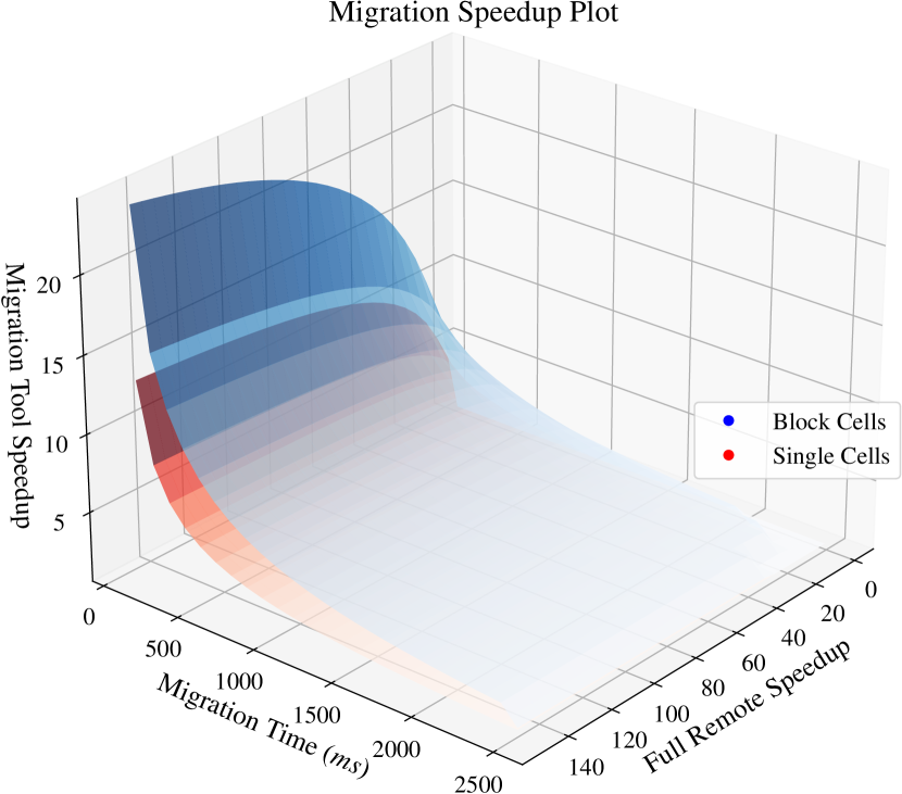
Figure 6: Speedup plot for TensorFlow guide notebook. This graph is similar to the synthetic loops notebook with the difference in terms of speedup of block-cell migrations. In this case, there are more cell migrations as the user creates shorter blocks of executed cells (Figure 4), then, the speedup is less significant.

Single-cell migrations present similar speedups for low migration times in both plots (see the dark red areas in Figures 5 and 6), however, the block-cell migration speedups are higher in the synthetic loops notebook (dark blue regions). There are two explanations for this: (i) the synthetic loops notebook presents bigger execution cycles when compared to the adapted Tensorflow guide notebook (Figure 4); this user cell execution behavior forces fewer migrations as the proposed solution executes larger blocks of cells, and (ii) the frequency of less computationally intensive cells is higher in the adapted Tensorflow guide notebook (Figure 7), making migrations to the local infrastructure more frequent.

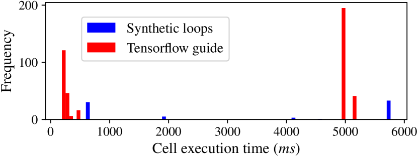
Figure 7: Cell execution times frequency graph. It shows the execution count and the relative frequency for executed cells in Synthetic loops and TensorFlow guide notebooks.

Figures 8 and 9 show the ratio between the speedups using block-cell and single-cell migration approaches for the two presented notebooks. For both figures, the speedup ratio is close to one when the full remote speedup is small and rises as the speedup increases. In other words, the block-cell migration approach takes more benefit from full remote speedups when compared to the single-cell migration approach. When we consider migration time increasing, the previous conclusion is not the same for both notebooks. For the adapted TensorFlow guide notebook, scenarios where the migration times are higher, the block-cell migration approach performs better when compared to the single-cell method. It happens as the block-cell migration approach performs fewer migrations than the single-cell migration method. For the synthetic loops notebook, migration time increases do not reflect directly into rises in the block-cell/single-cell speedups ratio as we would first infer. To explain this phenomenon, Figure 10, which presents a slice of Figure 8 with full remote speedup equals 150, shows the impact of migration counts for block-cell and single-cell migration policies on its speedups ratio. One can see when the proportion of block-cell and single-cell migrations remain constant (e.g., migration time between 1000 and 2000 milliseconds) the speedup ratio keeps increasing with the migration time increase, just like Figure 9. However, for this notebook, the cell execution times are more scattered when compared to the adapted TensorFlow guide notebook, which contains two main groups of execution times (Figure 7). These different groups of cell execution times change the number of migrations for both migration policies, altering the effect of migration time increasing on the speedup ratio (e.g., see migration time change from 900 to 1000ms). According to the results, we can see the following: (i) knowing the user cell execution flow can improve the migration policies and maintain a good compromise between execution costs and computational power during the interactive notebook construction, and (ii) the block-cell migration approach performs better than the single-cell migration policy as it leverages the user execution flow to improve the data exchange process.

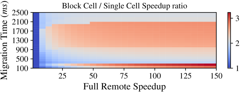
Figure 8: Block-cell/Single-cell speedup ratio for different values of migration times and remote infrastructure speedups related to synthetic loops notebook.

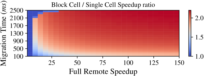
Figure 9: Block-cell/Single-cell speedup ratio for different values of migration times and remote infrastructure speedups related to TensorFlow guide notebook.

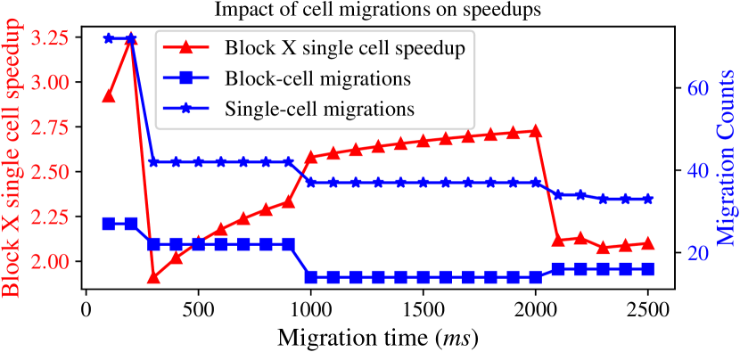
Figure 10: Impact of migration counts on block-cell/single-cell speedup ratios. We fixed the remote speed up to 150 times. Then, when the migration counts stay the same, the ratio keeps increasing with the rise of migration time. However, when the ratio changes, the relationship of Block X Single-cell speedups also changes.

Knowledge-aware policy. To evaluate this policy, we use a Deep Learning (DL) training Notebook as a motivating use case. In this example, the data scientist trains an image classifier DL model using the Cifar100 dataset. In this evaluation, we assess the hyperparameter number of epochs for a model training using the TensorFlow Keras library. In the initial state, the KB contains the information that, for the Cifar100 dataset, an estimate value for the number of epochs is $e=50$, which is manually informed by an expert (including the valid ranges). Nevertheless, $e=50$ may be sub or superestimating the optimal epoch value to migrate. For this reason, Algorithm 2 runs in background to build the training datasets with small candidate values for $e$. In this test, we set the migration time to 2 minutes and the maximum waiting time to 5 minutes, meaning that this is the time limit to build the initial dataset after the Migration Analyzer service identifies that a model is going to be fitted in the user’s Notebook. With the hardware in use in the experiments, the small number of epochs that can execute both locally and remotely while satisfying these constraints (and with a minimum amount of repetitions to analyze the standard deviation) is $\{1,2,3\}$. The times obtained for the local and remote environments for these numbers of epochs are used by the Migration Analyzer to train the local and remote ML models, using linear regression (see Fig. 11).

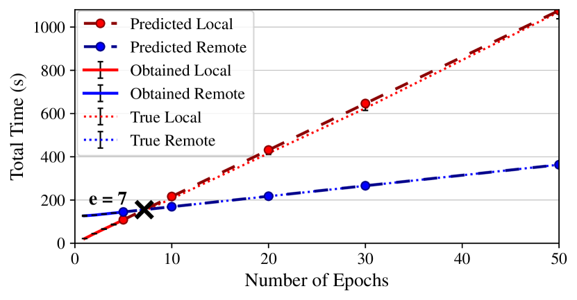
Figure 11: The algorithm automatically finds that for epochs $e>7$, the migration time pays off to migrate to an environment that runs 4.43x faster.

The red line represents the local times, whereas the blue line represents the remote times. The solid lines represent the obtained times for the small numbers of epochs $\{1,2,3\}$ executed and that were used as the training datasets for the regressors. To assess the accuracy of the predictions for greater numbers of epochs, we also execute these greater values to get their true total times (dotted lines in the plot). We expected that the predictions made by the regressors would have a good fit with the true lines, since the number of epochs is directly proportional to the training time and we are leaving all other hyperparameters constants. For this reason, the results confirm that the linear regressors are a simple and unexpensive solution to predict the total times for greater numbers of epochs and we also find that this holds even for a very small training dataset (3 obtained samples). The obtention of the total times repeated while the standard deviation of a minimum of two measurements was below 10% of the median. The obtained and true lines represent the median of these repetitions. We cannot repeat each measurement many times because each repetition counts for the user waiting time. Still, we see the prediction lines close to the true lines and the error bars, which represent the standard deviations of the repetitions, are very small. Furthermore, the lines for the remote times begin in a higher total time due to the migration time from the local to the remote host. However, since the remote host has a much more powerful hardware, particularly a GPU, and this DL training in Tensorflow using the Cifar100 dataset benefits from the GPU, the slope coefficient of the remote predicted line is much smaller (4.85) than the slope of the predicted local line (21.5), i.e., the local executions run 4.43x slower than the remote ones and, after the intersection point ($e=7$) between the two predicted lines, the migration pays off. This optimal epoch value is updated in the KB, which concludes the Algorithm 2. Finally, when the user executes the actual cell containing the model fitting content, passing the number epochs to train, the Migration Analyzer will use the recently updated optimal epoch value for the migration decision.

IV Related Work

There are several efforts related to our work, in particular around Jupyter-based technologies, provenance of interactive notebooks, and process migration. Here we highlight a few of them. Juric et al. [15] present a solution for checkpoint, restore, and live migration of Jupyter notebook sessions with JupyterHub. Their motivation is to reduce the resource wastage from idle user sessions, while also exploring the use of cheaper resource types, such as spot instances, to reduce costs hosting notebooks. With this capability, users can trigger complete session state checkpointing—which can be restored on the same or an alternative resource. Zonca and Sinkovits [16] describe strategies for deploying Jupyter notebooks at the Extreme Science and Engineering Discovery Environment (XSEDE). Their goal is to offer scalable hosting of Jupyter notebooks to a large number of users via a distributed infrastructure. One of the deployment strategies is to run Jupyter notebooks as jobs submitted to an HPC scheduler. Users can then login into JupyterHub and directly reach a cluster node. In this case, the job duration and other related configuration options are provided by the system administrator or set based on user preferences. Authors also explore Docker with Swarm mode to explore the capability of having a web server container running and not being affected by a node going down, as such container can be migrated to another node transparently.

Pimentel et al. [17] introduce a provenance system for interactive notebooks. Their motivation was that provenance support in notebooks was limited to visualization of intermediate results and code sharing, thus lacking the true history of all user interactivity. They proposed a new provenance approach for notebooks based on noWorkflow, which is a system to collect provenance from Python scripts. By doing so, they enable users to reason about such provenance data and debug their work. The noWorkflow system uses abstract syntax tree (AST) analysis to collect definitions in notebooks so a provenance graph can be generated. The same research team also performed a study on quality and reproducibility of Jupyter notebooks [18]. Also on provenance for Jupyter notebooks, Samuel and König-Ries [19] introduce a tool called ProvBook, which is a Jupyter extension to capture and view provenance data over the use of the notebooks. With the tool, users can compare current and previous experiments, querying sequences of executions using SPARQL. From a training perspective, Smith et al. [20] introduce a study on modeling student engagement with Jupyter notebooks. For their study, they consider metrics such as amount of time a student interacts with the notebook, and the number of times students execute and modify cells. Kery et al. [21] present a study on the usage of Jupyter notebooks and how data scientists track their experiments. Their focus was on the understanding of user behaviour, via a set of Jupyter notebooks and how data scientists track of their experiments. They focus on understanding user behaviour, via a set of interviews, rather than a tooling to collect such data. Process migration across multiple computing platforms is a well studied topic in several scenarios. For instance, there are efforts on seamlessly migrating virtual machines on wide area networks [22], optimization of context migration from mobile device to a cloud environment [23], and offloading computation from low-powered devices to remote resources accelerated by specialized hardware. In this context, Zhang and Pande [24] present a compiler framework to minimize migration cost of application processes in a mobile environment. They define a strategy that decides which parts of the program are good migration points (so the program can continue executing elsewhere). The process relies on the instrumentation of the application (to keep track of file operations, elapsed times, and memory usage) and on its profiling, from where the reaching graph for the application is built. From that graph, they (1) identify which files are accessed by which functions and (2) perform a backward data flow analysis to track global variable liveness. With the information learned about that program, the system computes the cost of migration at potential candidate points and, as last step, the migration handler is inserted in the code by the compiler so it can execute at run time.

Global variable liveness is also covered by Wang et al. [25], which use ASTs to analyze the quality of curated Python Jupyter Notebooks publicly available on a code hosting platform. They identify unused variables and deprecated functions by extracting these notebooks’ ASTs and searching them for assignment operations (i.e., Store nodes with names attached to them). Names associated with Store operations but lacking an association with a Load node are considered unused objects and flagged as such. The authors conclude that poor coding practices and lack of quality control is present in the majority of those Notebooks. Different from the related work, we use ASTs to find data dependencies in a Jupyter notebook’s code cells for automatic migration between execution environments, without requiring modifications of user code, while also capturing provenance information, all initiated from a JupyterLab extension that observes user interaction with notebooks.

V Conclusion

We proposed a migration tool for Jupyter notebooks that migrates code to most suitable computing platforms that increase user productivity. The tool requires no source code modification by the user, but only the installation of a JupyterLab extension. We also developed a component to reduce the notebook state to optimize migration processes. Our main findings developing the tool and performing experiments are that: (i) Jupyter-related technologies enable a rich environment to add features to increase user productivity; in our case, we enabled automatic execution of notebook cells in remote platforms, annotating cells explaining migration decisions; (ii) as notebooks are an extension of JSON, with JupyterLab allowing us to extract information on when cells are executed and modified, it is possible to build technology that explores the content of the cells and user interactions to enable better migration decisions; (iii) being an interactive platform, Jupyter notebooks cannot predict which variables may be accessed in future cells, hence memory consumption tends to grow over time; our AST-based notebook state reduction effectively works as a context-aware garbage collector without compromising the creation of new cells on that notebook; (iv) to find the right balance of computation power and monetary cost reduction, decisions on cell migration should leverage understanding of user context, that is, common sequences of cells normally executed by the user. This is because unnecessary migrations can be avoided compared to migration decisions only based on understanding computational needs of the current active notebook cell.

References

- [1] J. M. Perkel, “Why Jupyter is data scientists’ computational notebook of choice,” Nature, vol. 563, no. 7732, pp. 145–147, 2018.
- [2] H. Shen, “Interactive notebooks: Sharing the code,” Nature News, vol. 515, no. 7525, p. 151, 2014.
- [3] D. E. Knuth, “Literate programming,” The Computer Journal, vol. 27, no. 2, pp. 97–111, 1984.
- [4] K. J. Millman and F. Pérez, “Developing open-source scientific practice,” in Implementing Reproducible Research. Chapman & Hall/CRC, 2018.
- [5] T. Kluyver et al., Jupyter Notebooks – a publishing format for reproducible computational workflows, 2016.
- [6] D. Paine and L. Ramakrishnan, “Understanding interactive and reproducible computing with jupyter tools at facilities,” 2020.
- [7] K. M. Mendez et al., “Toward collaborative open data science in metabolomics using jupyter notebooks and cloud computing,” Metabolomics, 2019.
- [8] H. Nishimura et al., “Lattice Optimization Using Jupyter Notebook on HPC Clusters,” in IPAC, 2017.
- [9] R. Souza et al., “Workflow Provenance in the Lifecycle of Scientific Machine Learning,” arXiv preprint:2010.00330 [cs.DB], 2020.
- [10] T. Lebo et al. W3C PROV-O - The PROV Ontology. [Online]. Available: https://www.w3.org/TR/2013/REC-prov-o-20130430/
- [11] SpaceNet on Amazon Web Services (AWS), “Datasets,” The SpaceNet Catalog. Accessed on Apr 15, 2021. [Online]. Available: https://spacenet.ai/datasets
- [12] L. Deng, “The MNIST database of handwritten digit images for machine learning research [best of the web],” IEEE Signal Processing Magazine, vol. 29, no. 6, pp. 141–142, 2012.
- [13] R. Souza et al., “Efficient Runtime Capture of Multiworkflow Data Using Provenance,” in IEEE (eScience), 2019, pp. 1–10.
- [14] M. F. Moreno, R. Brandao, and R. Cerqueira, “Extending Hypermedia Conceptual Models to Support Hyperknowledge Specifications,” International Journal of Semantic Computing, 2017.
- [15] M. Juric et al., “Checkpoint, Restore, and Live Migration for Science Platforms,” arXiv preprint arXiv:2101.05782, 2021.
- [16] A. Zonca and R. S. Sinkovits, “Deploying Jupyter Notebooks at scale on XSEDE resources for Science Gateways and workshops,” in PEARC, 2018.
- [17] J. F. N. Pimentel, V. Braganholo, L. Murta, and J. Freire, “Collecting and analyzing provenance on interactive notebooks: when IPython meets noWorkflow,” in USENIX TaPP, 2015.
- [18] J. F. Pimentel et al., “A large-scale study about quality and reproducibility of jupyter notebooks,” in MSR, 2019.
- [19] S. Samuel and B. König-Ries, “ProvBook: Provenance-based Semantic Enrichment of Interactive Notebooks for Reproducibility,” in International Semantic Web Conference (P&D/Industry/BlueSky), 2018.
- [20] D. H. Smith IV et al., “Towards Modeling Student Engagement with Interactive Computing Textbooks: An Empirical Study,” in SIGCSE, 2021.
- [21] M. B. Kery, M. Radensky, M. Arya, B. E. John, and B. A. Myers, “The story in the notebook: Exploratory data science using a literate programming tool,” in CHI, 2018.
- [22] F. Travostino et al., “Seamless live migration of virtual machines over the MAN/WAN,” Future Generation Computer Systems, 2006.
- [23] Y. Li and W. Gao, “Minimizing context migration in mobile code offload,” IEEE Transactions on Mobile Computing, 2016.
- [24] K. Zhang and S. Pande, “Efficient Application Migration under Compiler Guidance,” SIGPLAN Not., vol. 40, no. 7, p. 10–20, Jun. 2005.
- [25] J. Wang, L. Li, and A. Zeller, “Better Code, Better Sharing: On the Need of Analyzing Jupyter Notebooks,” in ICSE-NIER, 2020.