Spin-dependent dark matter-electron interactions

Abstract

Detectors with low thresholds for electron recoil open a new window to direct searches of sub-GeV dark matter (DM) candidates. In the past decade, many strong limits on DM-electron interactions have been set, but most on the one which is spin-independent (SI) of both dark matter and electron spins. In this work, we study DM-atom scattering through a spin-dependent (SD) interaction at leading order (LO), using well-benchmarked, state-of-the-art atomic many-body calculations. Exclusion limits on the SD DM-electron cross section are derived with data taken from experiments with xenon and germanium detectors at leading sensitivities. In the DM mass range of 0.1–10 GeV, the best limits set by the XENON1T experiment: $\sigma_{e}^{(\textrm{SD})}<10^{-41}-10^{-40}\,\textrm{cm}^{2}$, are comparable to the ones drawn on DM-neutron and DM-proton at slightly bigger DM masses. The detector’s responses to the LO SD and SI interactions are analyzed. In nonrelativistic limit, a constant ratio between them leads to an indistinguishability of the SD and SI recoil energy spectra. Relativistic calculations however show the scaling starts to break down at a few hundreds of eV, where spin-orbit effects become sizable. We discuss the prospects of disentangling the SI and SD components in DM-electron interactions via spectral shape measurements, as well as having spin-sensitive experimental signatures without SI background.

Introduction

Direct searches of dark matter (DM) through its scattering with electrons have being a rapidly growing field in the past decade. With low-threshold capabilities of modern detectors in electron recoil (ER) and new ideas inspired by theoretical studies, the coverage of DM mass, $m_{\chi}$, has gradually been extended from sub-GeV towards increasingly lower reach (for a comprehensive overview, see, e.g., Ref. [1]). So far, most attention is given to the DM-electron interaction which is spin-independent (SI) of both DM and electrons. Various experiments have already set stringent exclusion limits on its cross section, $\sigma_{e}^{(\textrm{SI})}$, in the mass range of MeV to GeV [2, 3, 4, 5, 6, 7, 8, 9, 10, 11, 12, 13]. The current best limit above 30 MeV is set by XENON1T for their huge exposure mass and time [8, 14]; in the range of $1-30$ MeV, several experiments capitalizing the condensed phases of materials such as semiconductor silicon [9, 11] and germanium [12, 10] show potential improvements upon future scale-up. But, what about the spin-dependent (SD) interactions?

While there can be numerous models to motivate studies of SD DM-electron interactions from top down, a more straightforward, bottom-up approach is through nonrelativistic (NR) effective field theory [15, 16, 17, 18, 19, 20, 21, 22]. As most DM is believed to be cold, its velocity $v_{\chi}\sim 10^{-3}$ provides a natural parameter by which the DM interactions can be formulated as a series expansion. At leading order (LO), i.e., $v_{\chi}^{0}=1$, there are only two terms: $\mathbbm{1}_{\chi}\cdot\mathbbm{1}_{e}$ (SI) and $\vec{S}_{\chi}\cdot\vec{S}_{e}$ (SD), where $\mathbbm{1}$ and $\vec{S}$ are unity and spin operators, respectively. It is when matching these NR effective operators to their underlying theories that the generality and complementarity of such consideration shows its full power. For example, at the relativistic level, the SI term can come from either a scalar DM with a scalar-scalar coupling, or a fermionic DM with a scalar-scalar or vector-vector coupling to electrons; the SD term can come from a fermionic DM with an pseudovector-pseudovector or tensor-tensor coupling. As a result, null observations of them constrain different parts of the broad DM parameter space. On the other hand, an observation of the SD term would not only be a discovery of DM and a new interaction, but also exclude all scalar DM scenarios – this adds a stronger motivation to search for it.

The LO SD DM-nucleon interactions have been studied, though not as extensively as its SI counterpart, with good recent progress  [23, 24, 25, 26, 27, 28, 29, 30]. The best limits on the contact interactions with a neutron $(n)$ and a proton ($p$), in terms of total cross sections, are $\sigma_{n}^{(\textrm{SD})}<6.2\times 10^{-42}\,\textrm{cm}^{2}$ with $m_{\chi}=30\,\textrm{GeV}$ by XENON1T [28], and $\sigma_{p}^{(\textrm{SD})}<3.2\times 10^{-41}\,\textrm{cm}^{2}$ with $m_{\chi}=25\,\textrm{GeV}$ by PICO [29], respectively. Compared with the best limits of order $10^{-46}\,\textrm{cm}^{2}$ on the SI interactions, the huge order-of-magnitude difference is easily understood from the (almost) coherent contributions of $A\sim 100$ nucleons for the SI and a single unpaired nucleon for the SD case, respectively, in scattering amplitudes. On the other hand, because a typical atom is of size $\sim\mathring{\textrm{A}}$, a cold DM particle can not induce substantial coherent scattering with atomic electrons unless it is as light as $m_{\chi}\lesssim\textrm{MeV}$. Therefore, in direct searches of DM in the MeV-GeV mass range, one can anticipate constraints of similar orders on both LO SD and SI DM-electron interactions, for the latter has no coherent enhancement in scattering cross sections.

In this work, we study DM-atom scattering through the SD DM-electron interaction at leading order, using well-benchmarked, state-of-the-art atomic many-body approaches. Exclusion limits are derived from various data of xenon and germanium detectors. The limit on DM-electron cross section $\sigma_{e}^{(\textrm{SD})}<10^{-41}-10^{-40}\,\textrm{cm}^{2}$ with $m_{\chi}=0.1-10\,\textrm{GeV}$, set by XENON1T data, is comparable to the best ones on $\sigma_{n,p}^{(\textrm{SD})}$ mentioned above at slightly bigger $m_{\chi}$. Special attention is on the difference in detector responses to the SI and SD interactions, with spin-orbit effects being found to be the deciding factor. We discuss in the end several strategies for sub-GeV DM searches that can disentangle the SD and SI DM-electron interactions.

Formalism

At leading order (LO), the effective SD interaction between DM ($\chi$) and an electron ($e$) is

$$\mathscr{L}_{\textrm{SD}}^{(\textrm{LO})}=(c_{4}+d_{4}/q^{2})\left(\chi^{\dagger}\vec{S}_{\chi}\chi\right)\cdot\left(e^{\dagger}\vec{S}_{e}e\right)\,,$$ (1)

where the coupling constants $c_{4}$ and $d_{4}$ (following the convention of Refs. [15, 16]) are for the short- and long-range interactions, respectively; and $q$ the magnitude of the three-momentum transfer $\vec{q}$.

The unpolarized differential scattering cross section in the laboratory frame can be derived straightforwardly (see, e.g., Ref. [31]), and we focus only on the ionization processes that yield ER signals

$$\frac{d\sigma}{dT}^{(\textrm{ion})}=\frac{1}{2\pi v_{\chi}^{2}}\int qdq\,(\bar{c}_{4}+\bar{d}_{4}/q^{2})^{2}R_{\textrm{SD}}^{(\textrm{ion})}(T,q).$$ (2)

Note that for later convenience we redefine the coupling constants $(\bar{c}_{4},\bar{d}_{4})=\sqrt{\bar{s}_{\chi}/4}(c_{4},d_{4})$ by absorbing (i) the spin factor $\bar{s}_{\chi}=s_{\chi}(s_{\chi}+1)/3$, which results from an average of the initial, and a sum of the final DM spin states, with $s_{\chi}=1/2$ or $1$ applying to the case of a fermionic or vector DM particle, and (ii) the square of the electron spin $s_{e}=1/2$. The SD response function

$$R_{\textrm{SD}}^{(\textrm{ion})}(T,q)= \sum_{\mathscr{F}}\overline{\sum_{\mathscr{I}}}\sum_{j}\,|\braket{\mathscr{F}}{\sum_{i=1}^{Z}e^{i\vec{q}.\vec{r}_{i}}\sigma_{i,j}^{\textrm{D}}}{\mathscr{I}}|^{2}$$

$$\times\delta(E_{\mathscr{F}}-E_{\mathscr{I}}-T)\,,$$ (3)

involves a statistical average of the initial states $\ket{\mathscr{I}}$ and a sum of all final states $\ket{\mathscr{F}}$ allowed by energy conservation (imposed by the delta function). To incorporate relativistic effects in atoms, the electron spin operator is expressed by the $4\times 4$ Dirac spin matrices $\vec{\sigma}_{e}^{\textrm{D}}=2\vec{S}_{e}$, with $\vec{\sigma}^{\textrm{D}}=\gamma^{0}\vec{\gamma}=\left(\begin{array}[]{cc}\vec{\sigma}&0\\ 0&\vec{\sigma}\end{array}\right)$ where $\vec{\sigma}$ are the normal $2\times 2$ Pauli matrices. The transition operator contains all $Z$ electrons (the summation of $i$), and spin operators of orthogonal $j$-directions contribute incoherently (the summation of $j$).

Our evaluation of $R_{\textrm{SD}}^{(\textrm{ion})}$ proceeds similarly to our previous work on the SI case [14]. All the essential formulae, including those new to the SD case, are given in Appendix A . To emphasize once again the importance of relativistic and many-body physics, we also highlight therein the differences from NR, independent-particle approaches widely adopted in literature.

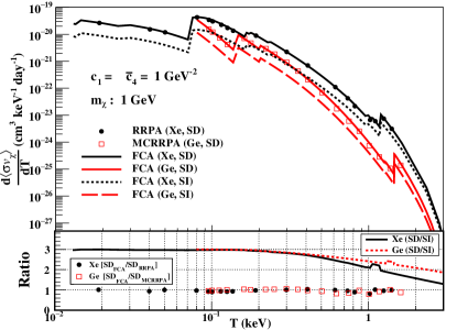
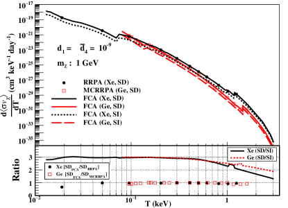
Figure 1: Top: Averaged velocity-weighted differential cross sections $\frac{d\left\langle\sigma v_{\chi}\right\rangle}{dT}$ for ionizations of xenon (black) and germanium (red) by leading-order spin-dependent (solid) and spin-independent (dashed) interactions of short (left) and long (right) range, at $m_{\chi}=$1 GeV and coupling constants of $c_{1}=\bar{c}_{4}=1/\textrm{GeV}^{-2}$ and $d_{1}=\bar{d}_{4}=10^{-9}$. Points in circles (open squares) are benchmark calculations by (MC)RRPA for xenon (germanium). Bottom: Lines are ratios of $\frac{d\left\langle\sigma v_{\chi}\right\rangle}{dT}$ with the SD to the SI interactions. Points in closed circles (open squares) are ratios of FCA to (MC)RRPA with the SD interaction for xenon (germanium).

While the computation of $R_{\textrm{SD}}^{(\textrm{ion})}$ involves completely different multipole operators from its SI counterpart $R_{\textrm{SI}}^{(\textrm{ion})}$, their definitions only differ formally in $R_{\textrm{SD}}^{(\textrm{ion})}$ having an additional spin operator $\vec{\sigma}^{\textrm{D}}$ and the associated summation of three directions. Therefore, before presenting our full numerical results, it is instructive to study the possible relationship between them. For the purpose, we define a scaling factor $\xi=R_{\textrm{SD}}^{(\textrm{ion})}/R_{\textrm{SI}}^{(\textrm{ion})}$.

First in Ref. [32], it was shown in DM scattering off free electrons that $\xi^{(0)}=3$. Later in Ref. [31], the same conclusion was reached for hydrogen-like atoms that $\xi^{(\textrm{H})}=3$. Recently, in Ref. [33], the same conclusion was generalized to many-electron atoms with two conditions: (i) the electron basis wave functions are labeled by the principle (for bound states) or energy (for continuum states), orbital, and magnetic quantum numbers: $n$ or $k$ (with $E=k^{2}/2m_{e}$), $l$, $m_{l}$, and (ii) the final states are purely one-particle-one-hole excitations from the ground state. In such a NR, purely mean-field framework, it also yields that $\xi^{(\textrm{NR})}=3$. Because a NR electron’s orbital and spin wave functions are factorized, the scaling factor of 3 can be heuristic deducted from the multiplicity of the $\vec{\sigma}$ (for the SD case) over the unity (for the SI case) operator, when the transition involves only one independent electron.

However, as there is spin-orbit interaction (SOI) in atoms, this scaling relation can only be approximate at best. Its effects show up in all parts of the response function. First, the SOI causes the energy shift of two electron states of same $l$ but different total angular momenta $j=l\pm 1/2$, so the energy conserving delta functions are different. Second, the electron basis wave functions (which are best solved by relativistic mean field methods), their associated one-electron matrix elements, and the density matrix (which contains the weights of all atomic configurations that can be mixed by the residual interaction) all have explicit dependence on $j$. Therefore, one chief goal of this paper is to quantify to what extent that $\xi\approx 3$ is a good approximation to apply in DM-atom scattering.

It should be pointed out that the analogous behavior for DM-nucleus scattering is rather different. Unlike the atomic SOI, which is electromagnetic with its strength characterized by the fine structure constant $\alpha_{\textrm{EM}}\approxeq 1/137$, the nuclear SOI is a component of the nuclear strong interaction, and its strength is of the order of the strong coupling constant $\alpha_{\textrm{S}}\sim 1$. Consequently, there is no such simple scaling in DM-nucleus scattering through the SD and SI DM-nucleon interactions (see, e.g., Ref. [16]).

Results

To get a prediction for the event rate at a detector with $N_{T}$ atoms

$$\frac{dR}{dT}=\frac{\rho_{\chi}\,N_{T}}{m_{\chi}}\frac{d\braket{\sigma v_{\chi}}}{dT}\,,$$ (4)

the differential cross section is weighted and averaged by the standard Maxwell-Boltzmann velocity distribution of DM [34], $f(\vec{v}_{\chi})$,

$$\frac{d\braket{\sigma v_{\chi}}}{dT}=\int_{v_{\min}}^{{v_{\textrm{max}}}}d^{3}v_{\chi}f(\vec{v}_{\chi})v_{\chi}\frac{d\sigma}{dT}\,,$$ (5)

with conventional choices of DM parameters (same as in Ref. [14]): the local density $\rho_{\chi}=0.4$ GeV/cm³, circular velocity $v_{0}=220\,\textrm{km/s}$, escape velocity $v_{\textrm{esc}}=544\,\textrm{km/s}$, averaged Earth relative velocity $v_{E}=232\,\textrm{km/s}$ so that $v_{\textrm{max}}=v_{\textrm{esc}}+v_{E}$, and minimum $v_{\min}=\sqrt{2T/m_{\chi}}$. We follow the same efficient velocity average scheme as in Refs. [32, 35] via an eta function $\eta(v_{\textrm{min}})=\left\langle v_{\chi}^{-1}\theta(v-v_{\textrm{min}})\right\rangle$  [34, 36]. This simplification has been explicitly verified in Ref. [14] for the same kinematic region.

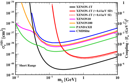
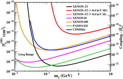
Figure 2: Top: Exclusion limits at 90% C.L. on the spin-dependent short- (left) and long- (right) range DM-electron interactions as functions of $m_{\chi}$ derived from data of CDMSlite [24], XENON10 [2], XENON100 [3], XENON1T [8], and PandaX-II [13] data. The SD and SI limits of XENON1T at 400 eV threshold are depicted as solid and dotted red lines, respectively, to illustrate their expected recoil spectral shape are different. 

In Fig. 1, the results of $d\braket{\sigma v_{\chi}}/dT$ are shown for the cases with $m_{\chi}=1\,\textrm{GeV}$, $c_{1}=\bar{c}_{4}=1/\textrm{GeV}^{-2}$, and $d_{1}=\bar{d}_{4}=10^{-9}$. The fully many-body calculations through (multiconfiguration) relativistic random phase approximation, (MC)RRPA, are performed at a few points (for them being computer-time-consuming) labeled by circles (open squares) for xenon (germanium) atoms as benchmarks. The main results in solid curves are obtained from a more efficient approach: the frozen core approximation (FCA), which is in the spirit of an independent particle approximation but with a more realistic mean field to compute the ionized electron wave function (details in Ref. [14]). In general, FCA shows good agreement with (MC)RRPA benchmark points except near edge energies. Considering the $5\%$ accuracy of (MC)RRPA achieved in photoabsorption cross sections with $T\geq$12 and 80 eV for xenon [37] and germanium [38, 39], respectively, we conservatively assign an overall theory error of $20\%$. (The theory error can be reduced to 5%, if we perform (MC)RRPA calculations throughout the work without the limitation of computer resources.) Complete data of $d\braket{\sigma v_{\chi}}/dT$ with different $m_{\chi}$ are provided in the folder of ancillary files.

Data from CDMSlite [24], XENON10 [2], XENON100 [3], XENON1T [8], and PandaX-II [13] are analyzed against the theory predictions of $dR/dT$ in the same way as in Ref. [14]). In Fig. 2, the exclusion limits on the coupling constants $\bar{c}_{4}$ and $\bar{d}_{4}$, and equivalently the SD DM-electron total cross sections $\sigma_{e}^{(\textrm{SD})}=3\bar{c}_{4}^{2}\mu_{\chi e}^{2}/\pi$ and $\bar{\sigma}_{e}^{(\textrm{SD})}=3\bar{d}_{4}^{2}\mu_{\chi e}^{2}/\left(\pi(m_{e}\alpha)^{4}\right)$, where $\mu_{\chi e}=m_{\chi}m_{e}/(m_{\chi}+m_{e})$, are presented on the right and left $y$-axis, respectively. For $m_{\chi}$ larger than 42 and 140 MeV, XENON1T provides the most stringent limits for the short- and long-range interactions, respectively, with its ton-year scale exposure. Particularly in the range between $0.1-10\,\textrm{GeV}$, the limits on $\sigma_{e}^{(\textrm{SD})}<10^{-41}-10^{-40}\,\textrm{cm}^{2}$ are of similar order of magnitude as the ones of $\sigma_{n,p}^{(\textrm{SD})}$ at slightly bigger $m_{\chi}$. This is an important complement to mainstream searches of weakly-interacting massive particles through DM-nucleus scattering: not only because of some overlapping in mass range (1-10 GeV), but also for classes of DM which can be both hadro- and lepto-phillic. For smaller $m_{\chi}$ down to 10 MeV, PandaX-II instead set better limits because of its lower ER threshold at $80\,\textrm{eV}$. It defines the exclusion boundary at low $m_{\chi}$ for having lower background $\sim 2.64\times 10^{-4}\,\textrm{cpd/kg/keV}$ compared to $\sim 0.2$ of XENON10, despite the latter has an even lower threshold at $13.8\,\textrm{eV}$.

We emphasize here the derived exclusion limits depend critically on the theory predictions for the DM scattering event rates. Substantial differences exist between our relativistic many-body approach and several NR mean-field approaches Refs. [35, 2, 3, 4, 33] including the package QEdark that was used in the data analyses of Refs. [8, 13]. Detailed comparisons, reasons that cause the differences, and justifications of our approach are presented in Ref. [14]. Based on similar arguments, one would generically anticipate weaker limits on the short-range interaction in the high-mass region, and tighter limits on the long-range interaction in the low-mass region, when above-mentioned approaches are applied. The main reasons are: (i) the relativistic effects substantially increase the scattering event rate at high $T$, and (ii) the many-body effects play an important role at all distances, including the Coulomb screening at long distances which substantially decrease the scattering rate at very low $T$.

Not included in our data analyses are several low-threshold semiconductor experiments, which already set limits on $\sigma_{e}^{(\textrm{SI})}$ below 10 MeV [6, 5, 7, 11, 9, 10] and have the potential to compete with liquid noble-gas detectors above the 10 MeV region, particularly for the long-range interactions, in the future. The associated many-body physics of condensed matter is beyond the scope of this work, but has been taken in Refs. [40, 41, 42, 43, 44, 45, 46] for the SI interaction, and recently in Refs. [47, 22, 45, 46] that also include the SD interactions. Currently, there are discrepancies among predictions from different theoretical schemes.

Disentanglement of SD and SI interactions

Conventional DM detectors only measure recoil energy. Detector responses to SI and SD signatures must be different in order to disentangle them. Therefore, if the NR scaling $\xi^{(\textrm{NR})}=3$ is valid, the SD and SI signals are indistinguishable in the measurable recoil energy spectrum shapes and the exclusion limits of $\sigma_{e}^{(\textrm{SD})}$ and $\sigma_{e}^{(\textrm{SI})}$ would have identical $m_{\chi}$ dependence.

In the bottom panel of Fig. 1, this statement is examined through the $\bar{\xi}$ parameter, which is the ratio of $\frac{d\left\langle\sigma v_{\chi}\right\rangle}{dT}$ with the SD to the SI interaction, for the case of $m_{\chi}=1\,\textrm{GeV}$. The overbar in $\bar{\xi}$ indicates the responses functions are integrated over $q$ and averaged over the DM flux in $\frac{d\left\langle\sigma v_{\chi}\right\rangle}{dT}$. At $T\lesssim 200\,\textrm{eV}$, the scaling relation $\bar{\xi}\approx 3$ works well for both xenon and germanium. The scaling deviation starts to grow as $T$ increases, and the larger deviations in xenon than germanium demonstrates the effects of a stronger SOI in an atom of higher $Z$. We note that the SOI is only part of the relativistic corrections in atoms. Therefore, even though it has been shown that relativistic corrections become sizable for $T\gtrsim 200\,\textrm{eV}$ in DM-xenon scattering [14], the departure of $\bar{\xi}$ from the NR prediction $\bar{\xi}^{\textrm{(NR)}}=3$ is comparatively modest.

It follows that precision spectral shape measurements at high energy allow SD and SI to be distinguished in the case of positive discovery signals. As SD limits are driven by detector thresholds lower than 200 eV, the exclusion curves of Fig. 2 differ only slightly from the ones for SI given in Fig. 2 of Ref. [14]. If a higher cutoff is applied, as the example shown in Fig. 2 with 400-eV cutoff to XENON1T data, noticeable difference shows up.

There are intriguing possibilities of experimental signatures unique to SD interactions without SI background. For example, in a spin polarizable target and with known spin states of the ionized electrons, only part of the SD interaction $\sum_{\lambda=\pm 1}(-1)^{\lambda}S_{\chi,\lambda}S_{e,-\lambda}$ (where $\lambda$ denotes the spherical component) can generate signals as spin-flips. There are intense recent interests to seek solutions in condensed phases of matter which have natural spin, or magnetic, order. For instance, a ferrimagnetic material: yttrium iron garnet has been proposed as a candidate target [47, 22] for light DM searches with $m_{\chi}\leq 10\,\textrm{MeV}$. The SD DM-electron interaction can perturb this spin system and generate magnons, which are the low-energy quanta of spin waves and experimentally measurable.

Motivated by the role of SOI, another approach is to realize experimental configurations where spins couple strongly to orbital angular momenta. For atoms, the fine structure constant is fixed, so that SOI enhancement can only be found in the inner-shell electrons, which have higher ionization energies. The novel Dirac materials do have the desired property that the effective fine structure constants can be larger than $\alpha_{\textrm{EM}}$. Take graphene as an example: a naive dimensional analysis yields $\alpha_{g}=\alpha_{\textrm{EM}}/v_{F}\approx 2.2$, adopting a generic Fermi velocity at Dirac cone $v_{F}\approx 10^{6}\,\textrm{m/s}$. While recent calculations [48] and measurements [49, 50] reported smaller values in between 0.1 and 1 (mostly due to the suppression by Coulomb screening), they are still significantly bigger than $\alpha_{\textrm{EM}}$. The smallness of $v_{F}$ compared to the speed of light is the most important factor that lowers the bar to reach the relativistic limit. Unfortunately, the intrinsic SOI in graphene is found to be small [51], so whether it could generate a sufficiently different SD response requires more study. More promising candidates are topological insulators [52, 53] and transition-metal dichalcogenides [54], whose structures critically depend on SOIs. In addition, among a few Dirac materials being proposed to search for SI DM-electron interactions, the semimetal $\textrm{ZrTe}_{5}$ [55, 56, 57] and organic crystal $(\textrm{BEDT-TTF})\cdot\textrm{Br}$ [58] show corrections from SOIs in band structure calculations.

Summary

The SD DM-electron interactions is an important, but less-attended subject in direct DM searches. Its studies complement the very active research on the SI interactions, and together they can provide a more comprehensive understanding about the nature of DM and its interactions with matter. We derive in this paper, for the first time, limits on the SD DM-electron cross sections at leading order with state-of-the-arts atomic many-body calculations and current best experiment data. As a result of spin-orbit interaction, the spectral shapes of SD and SI recoil spectra differ at high energies, which provides a way of differentiating them experimentally. In addition, signals unique to SD interactions and systems of enhanced SOIs that can be found in novel phases of matter may offer more direct experimental probes for SD from sub-GeV DM searches in the future.

Appendix A Atomic Many-body Response Functions 

It is a well-acknowledged fact that a detector’s response to scattering of nonrelativistic sub-GeV DM involves many-body physics at atomic, molecular, or condensed matter scale, depending on the configuration of a detector. In this Appendix, we summarize the important steps and formulae in a truly many-body calculation of the atomic response functions, and illustrate the differences to approaches based solely on independent particle pictures, either relativistically or non-relativistically. We shall follow the notations and terminology of Ref. [16] (a seminal work on the nuclear responses to DM-nucleus scattering) as much as possible. However, a necessary addition is using Dirac spinors for electrons, as relativistic effects are important and manifest in atomic physics. A further note is while a formulation in molecular or condensed matter systems proceeds similarly in spirit, there are substantial changes of basic elements and notations which we leave for future work.

For brevity, consider only the short-range DM-electron interactions

$$\mathscr{L}^{(\textrm{LO})}=c_{1}\left(\chi^{\dagger}\mathbbm{1}_{\chi}\chi\right)\cdot\left(e^{\dagger}\mathbbm{1}_{e}\right)+c_{4}\left(\chi^{\dagger}\vec{S}_{\chi}\chi\right)\cdot\left(e^{\dagger}\vec{S}_{e}e\right)\,,$$ (6)

with both leading-order SI ($c_{1}$) and SD ($c_{4}$) terms included. The unpolarized differential scattering cross section in the laboratory frame is given by

$$\frac{d\sigma}{dT}^{(\textrm{ion})}=\frac{1}{2\pi v_{\chi}^{2}}\int qdq\,c_{1}^{2}R^{(\textrm{SI})}(T,q)+\bar{c}_{4}^{2}R^{(\textrm{SD})}(T,q)\,,$$ (7)

where $\bar{c}_{4}=\sqrt{s_{\chi}(s_{\chi}+1)/12}\,c_{4}$ that absorbs the factors due to DM spin, $s_{\chi}$, and electron spin $s_{e}=1/2$. The SI and SD detector responses are encoded in two functions

$$R_{\textrm{SI}}^{(\textrm{ion})}(T,q)= \sum_{\mathscr{F}}\overline{\sum_{\mathscr{I}}}\,|\braket{\mathscr{F}}{\sum_{i=1}^{Z}e^{i\vec{q}.\vec{r}_{i}}}{\mathscr{I}}|^{2}\,\delta(E\ldots)\,,$$ (8a)

$$R_{\textrm{SD}}^{(\text{ion})}(T,q)= \sum_{\mathscr{F}}\overline{\sum_{\mathscr{I}}}\sum_{k}\,|\braket{\mathscr{F}}{\sum_{i=1}^{Z}e^{i\vec{q}.\vec{r}}\sigma_{i,k}^{\mathrm{D}}}{\mathscr{I}}|^{2}\,\delta(E\ldots)\,,$$ (8b)

where the delta function imposes energy conservation $E_{\mathscr{F}}=E_{\mathscr{I}}+T$.

A substantial simplification to the problem can usually be achieved by multipole expansion. First, because total angular momentum and its $z$-projection, are good quantum numbers, so we label the initial and final states as $\ket{\mathscr{I}}=\ket{I,J_{I}M_{J_{I}}}$ and $\ket{\mathscr{F}}=\ket{F,J_{F}M_{J_{F}}}$, respectively, where $I$ and $F$ are collective labels for other quantum numbers. Second, each multipole operator has its definite spherical rank, $J$, component, $M_{J}$, and parity, so the selection rules help to organize all allowed transitions in a systematic way. Third, by the Wigner-Eckart theorem, the summation over $M_{J_{F}}$, $M_{J_{I}}$, and $M_{J}$ can be carried out easily, and what remain to be calculated are the reduced matrix elements. Most important of all, for low energy processes, the expansion in spherical rank converges efficiently.

Following the notation of Ref. [16], the SI and SD response functions can now be decomposed as

$$R_{\textrm{SI}}^{(\textrm{ion})}(T,q)= \sum_{FJ_{F}}\overline{\sum_{IJ_{I}}}\frac{4\pi}{2J_{I}+1}\sum_{J=0}\left|\left\langle F,J_{F}\left\|\hat{M}_{J}(q)\right\|I,J_{I}\right\rangle\right|^{2}\delta(E\ldots)\,,$$ (9a)

$$R_{\textrm{SD}}^{(\textrm{ion})}(T,q)= \sum_{FJ_{F}}\overline{\sum_{IJ_{I}}}\frac{4\pi}{2J_{I}+1}\left\{\sum_{J=1}\left|\left\langle F,J_{F}\left\|\hat{\Sigma}_{J}(q)\right\|I,J_{I}\right\rangle\right|^{2}\right.$$

$$\left.+\sum_{J=1}\left|\left\langle F,J_{F}\left\|\hat{\Sigma}_{J}^{{}^{\prime}}(q)\right\|I,J_{I}\right\rangle\right|^{2}+\sum_{J=0}\left|\left\langle F,J_{F}\left\|\hat{\Sigma}_{J}^{{}^{\prime\prime}}(q)\right\|I,J_{I}\right\rangle\right|^{2}\right\}\delta(E\ldots)\,,$$ (9b)

and the relevant four types of multipole operators are

$$\hat{M}_{J}^{M_{J}}(q) =\sum_{i=1}^{Z}j_{J}(qr_{i})Y_{J}^{M_{J}}(\Omega_{r_{i}})\,,$$ (10a)

$$\hat{\Sigma}_{J}^{M_{J}}(q) =\sum_{i=1}^{Z}j_{J}(qr_{i})\vec{Y}_{JJ}^{M_{J}}(\Omega_{r_{i}})\cdot\vec{\sigma}_{i}^{\textrm{D}}\,,$$ (10b)

$$\hat{\Sigma}_{J}^{{}^{\prime}M_{J}}(q) =\sum_{i=1}^{Z}\left\{-\sqrt{\frac{J}{2J+1}}j_{J+1}(qr_{i})\vec{Y}_{JJ+1}^{M_{J}}(\Omega_{r_{i}})+\sqrt{\frac{J+1}{2J+1}}j_{J-1}(qr_{i})\vec{Y}_{JJ-1}^{M_{J}}(\Omega_{r_{i}})\right\}\cdot\vec{\sigma}_{i}^{\textrm{D}}\,,$$ (10c)

$$\hat{\Sigma}_{J}^{{}^{\prime\prime}M_{J}}(q) =\sum_{i=1}^{Z}\left\{\sqrt{\frac{J+1}{2J+1}}j_{J+1}(qr_{i})\vec{Y}_{JJ+1}^{M_{J}}(\Omega_{r_{i}})+\sqrt{\frac{J}{2J+1}}j_{J-1}(qr_{i})\vec{Y}_{JJ-1}^{M_{J}}(\Omega_{r_{i}})\right\}\cdot\vec{\sigma}_{i}^{\textrm{D}}\,,$$ (10d)

where $j_{J}(qr)$ is the spherical Bessel function, $Y_{J}^{M_{J}}(\Omega_{r})$ the spherical harmonics of solid angle $\Omega_{r}$, and $\vec{Y}_{JL}^{M_{J}}(\Omega_{r})$ the vector spherical harmonics formed by recoupling of $Y_{L}^{M_{L}}(\Omega_{r})$ and the unit vector $\hat{r}$, whose spherical projection is proportional to $Y_{1}^{\lambda}$.

A general feature of all these matrix elements to be computed is they involve many-body states $\ket{\mathscr{I}}$ and $\ket{\mathscr{F}}$, but the operators are one-body, i.e, only one electron makes transition at one time. Such matrix elements of a generic one-body operator $\hat{O}^{(1)}=\sum_{i}\hat{o}^{(i)}$ can be compactly written by second quantization that

$$\braket{\mathscr{F}}{\hat{O}^{(1)}}{\mathscr{I}}=\sum_{\alpha\beta}\Psi_{\mathscr{FI}}(\alpha,\beta)\braket{\alpha}{\hat{o}}{\beta}\,,$$ (11)

where the one-body density matrix

$$\Psi_{\mathscr{FI}}(\alpha,\beta)=\braket{\mathscr{F}}{\hat{c}_{\alpha}^{\dagger}\hat{c}_{\beta}}{\mathscr{I}}$$ (12)

gives the statistical weight of annihilating an electron with a quantum state labeled by $\beta$ and creating an electron with a quantum state labeled by $\alpha$ in this transition, and the total transition amplitude is the weighted sum of each single-particle transition with an amplitude given by $\braket{\alpha}{\hat{o}}{\beta}$ (the reference to the $i$th electron is dropped because electrons are identical.

Implementing the above scheme to a spherical basis with spherical operators is standard but too lengthy to reproduce here, but we should mention two basic ingredients. First, all single-particle states have good quantum labels of total angular momentum, so one can label them as $\ket{\alpha}=\ket{aj_{a}m_{j_{a}}}$ and $\ket{\beta}=\ket{bj_{b}m_{j_{b}}}$. Second, by recoupling the creation and annihilation operator $\hat{c}_{\alpha}^{\dagger}$ and $\hat{c}_{\beta}$, a spherical tensor operator of rank $J$ and component $M_{J}$ can be formed

$$[\hat{c}_{\alpha}^{\dagger}\otimes\hat{c}_{\beta}]_{J}^{M_{J}}=\sum_{m_{j_{a}}m_{j_{b}}}\braket{j_{a}j_{b};JM_{J}}{j_{a}j_{b};m_{j_{a}}m_{{}_{j_{b}}}}\hat{c}_{\alpha}^{\dagger}\hat{c}_{\beta}\,,$$ (13)

where the braket is the standard Clebsch-Gordan coefficient. Consequently, the reduced matrix element of a spherical operator can be recast as

$$\braket{F,J_{F}}{\hat{O}_{J}^{(1)}}{I,J_{I}}=\frac{1}{\sqrt{2J+1}}\sum_{aj_{a}bj_{b}}\bar{\Psi}_{FJ_{F};IJ_{I}}^{J}(aj_{a},bj_{b})\braket{aj_{a}}{\hat{o}_{J}}{bj_{b}}\,,$$ (14)

and the resulting density matrix is also reduced

$$\bar{\Psi}_{FJ_{F},IJ_{I}}^{J}(aj_{a},bj_{b})=\left\langle F,J_{F}\left\|[\hat{c}_{\alpha}^{\dagger}\otimes\hat{c}_{\beta}]_{J}\right\|I,J_{I}\right\rangle\,,$$ (15)

in the sense that it no longer depends on total angular momentum substates $m_{j_{a}}$ and $m_{j_{b}}$, and the spherical multipole component $M_{J}$.

At this point we should note that as long as many-body wave functions can be obtained exactly, the choice of a complete set of single-particle basis states $\{\ket{\alpha},\ket{\beta},\ldots\}$ is irrelevant, because the density matrix is also known exactly. However, this does not happen in practical cases, and the arts of many-body methods is mostly about choosing good sets of basis states and solving the density matrix reliably. The approach by Ref. [16], the nuclear shell model, is built upon a simple basis spanned by the harmonic oscillator eigenstates, which have nice properties that yield algebraic results of single-particle matrix elements. This simplistic mean field is compensated by diagonalizing the residual interaction in a large, but still truncated, model space with proper care in using the effective operators. Our approach, the (multiconfiguration) relativistic random phase approximation ((MC)RRPA), proceeds in a rather different direction. The mean field is first solved self-consistently by the Dirac-Hartree-Fock equation, so the single-particle basis states are optimized, i.e, they already include a large part of many-body physics. Then the effects due to the residual interactions are accounted for by the random phase approximation. The resulting density matrices, though not as dense as the ones of shell model approaches, are certainly not sparse when residual correlation induces substantial configuration mixing.

A.1 Independent Particle Approximation

Full-scale many-body calculations of the atomic responses by (MC)RRPA, or other methods that take residual interactions into account, usually have high demand of computing resources. Therefore, it is desirable to seek approximations that perform reasonably good but more efficiently. For the purpose, the independent particle approximation (IPA) based on mean field approaches serves as a good starting point.

In such a picture, the ground state of an atom is approximated by filling all electrons to lowest $Z$ single-particle orbitals, which are solutions of the mean field equation, and the resulting many-body wave function, as a Slater determinant (or a linear combination of several equivalent configurations for open-shell atoms), can successfully describe a lot, if not all, static ground state properties of an atom. When considering the action of a one-body operator on this assembly of $Z$ noninteracting electrons, called core electrons, then the excited state is simply one electron leaving the core and occupying a higher energy level (for ionization, a positive-energy state in continuum). Conventionally, this final state is called a one-particle-one-hole (1p1h) excitation of the initial ground state, which is taken to be the physical vacuum $\ket{0}$ of zero particle and zero hole, and also zero total angular momentum $J_{I}=0$. A final state of $J_{F}=J$ that corresponds to one bound electron in the orbital $\ket{n_{i}l_{i}j_{i}}$ being ionized to a continuum orbital $\ket{k_{f}l_{f}j_{f}})$ can be completely specified as $\ket{(k_{f}l_{f}j_{f})(n_{i}l_{i}j_{i})^{-1},J_{F}=J}=\ket{\textrm{1p1h};J}$. As a result, the density matrix in the independent particle picture is extremely simple:

$$\left\langle\textrm{1p1h};J\left\|[\hat{c}_{\alpha}^{\dagger}\otimes\hat{c}_{\beta}]_{J}\right\|0;0\right\rangle=\sqrt{2J+1}\delta_{a,k_{f}l_{f}}\delta_{j_{a}j_{f}}\delta_{b,n_{i}l_{i}}\delta_{j_{b}j_{i}}\,,$$ (16)

and the many-body matrix element is reduced to the one with single-particle states

$$\braket{\textrm{1p1h};J}{\hat{O}_{J}^{(1)}}{0;0}=\braket{k_{f}l_{f}j_{f}}{\hat{o}_{J}}{n_{i}l_{i}j_{i}}\,,$$ (17)

where $|j_{f}-j_{i}|\leq J\leq j_{f}+j_{i}$.

The spin-angular parts of the relevant single-particle matrix elements can be worked out algebraically as follows. First, we express the relativistic single-particle orbital functions in coordinate space as

$$\phi_{\varepsilon ljm}(\vec{r})=\frac{1}{r}\left(\begin{array}[]{c}g_{\varepsilon lj}(r)\mathscr{Y}_{jl}^{m}(\Omega_{r})\\ -if_{\varepsilon lj}(r)(\vec{\sigma}\cdot\hat{r})\mathscr{Y}_{jl}^{m}(\Omega_{r})\end{array}\right)\,,$$ (18)

where $\varepsilon$ refers to $n\,(k)$ for the bound (free) electron, and $\mathscr{Y}_{jl}^{m}(\Omega_{r})$ the spin-angular function. Then the reduced matrix elements are simplified by the following two formulae:

$$\braket{\varepsilon_{f}l_{f}j_{f}}{j_{J}(qr)Y_{J}(\Omega_{r})}{\varepsilon_{i}l_{i}j_{i}} =\frac{(-1)^{J+j_{i}+1/2}}{\sqrt{4\pi}}[l_{f}][l_{i}][j_{f}][j_{i}][J]\left\{\begin{array}[]{ccc}l_{f}&j_{f}&\nicefrac{{1}}{{2}}\\ j_{i}&l_{i}&J\end{array}\right\}\left(\begin{array}[]{ccc}l_{f}&J&l_{i}\\ 0&0&0\end{array}\right)\times\left\langle\varepsilon_{f}l_{f}j_{f}\left|j_{J}(qr)\right|\varepsilon_{i}l_{i}j_{i}\right\rangle$$ (19e)

$$\braket{\varepsilon_{f}l_{f}j_{f}}{j_{L}(qr)\vec{Y}_{JL}(\Omega_{r})\cdot\vec{\sigma}^{\textrm{D}}}{\varepsilon_{i}l_{i}j_{i}} =\frac{(-1)^{l_{f}}\sqrt{6}}{\sqrt{4\pi}}[l_{f}][l_{i}][j_{f}][j_{i}][L][J]\left\{\begin{array}[]{ccc}l_{f}&l_{i}&L\\ \nicefrac{{1}}{{2}}&\nicefrac{{1}}{{2}}&1\\ j_{f}&j_{i}&J\end{array}\right\}\left(\begin{array}[]{ccc}l_{f}&L&l_{i}\\ 0&0&0\end{array}\right)\times\left\langle\varepsilon_{f}l_{f}j_{f}\left|j_{L}(qr)\right|\varepsilon_{i}l_{i}j_{i}\right\rangle$$ (19k)

where the shorthand notation $[x]=\sqrt{2x+1}$, and the standard forms of the Wigner 3-$j$, 6-$j$, and 9-$j$ symbols are used.

The most important structure information is contained in the radial integrals

$$\left\langle\varepsilon_{f}l_{f}j_{f}\left|j_{J}(qr)\right|\varepsilon_{i}l_{i}j_{i}\right\rangle=\int dr\,j_{J}(qr)\,(g_{\varepsilon_{f}l_{f}j_{f}}(r)g_{\varepsilon_{i}l_{i}j_{i}}(r)+f_{\varepsilon_{f}l_{f}j_{f}}(r)f_{\varepsilon_{i}l_{i}j_{i}}(r))\,,$$ (20)

which depend on the single-particle orbital wave functions. For the electrons in the core, as the mean field methods based on variational principles are designed to get a best approximation for the ground state energy, the resulting wave functions can be taken with certain confidence. However, it is more problematic for the ionized electron, and such a highly excited state goes beyond the reach of conventional mean field design. There are many methods applied to DM-atom scattering, including plane wave, hydrogen-like, and frozen core approximations. We refer readers to Ref. [14] for more discussions and comparison of these methods, and only point out here that even though our main results in this paper are obtained with a frozen core approximation (FCA), the latter approach is justified by a few benchmark calculations using (MC)RRPA.

A.2 Nonrelativistic Limit

By further taking the nonrelativistic (NR) limit to the above independent particle approximation, we now show explicitly how our formulation can be reduced to the conventional form widely used in the literature, and recover the NR scaling factor $\xi^{(\textrm{NR})}=3$.

In numerical computations, the NR limit can be implemented by taking the speed of light to infinity. Theoretically, the most important features are (i) the Dirac spinor now has a vanishing small component and collapses to a Pauli spinor, i.e., all functions $f_{\varepsilon lj}(r)$ can be taken to zero, and (ii) the radial wave functions now only depends on $\varepsilon$ and $l$, since there is no longer spin-orbit interaction to break the $j=l\pm 1/2$ degeneracy. As a result, the only change in our formulation is in the radial integral

$$\left\langle\varepsilon_{f}l_{f}j_{f}\left|j_{J}(qr)\right|\varepsilon_{i}l_{i}j_{i}\right\rangle\rightarrow\left\langle\varepsilon_{f}l_{f}\left|j_{J}(qr)\right|\varepsilon_{i}l_{i}\right\rangle_{(\textrm{NR})}=\int dr\,j_{J}(qr)\,u_{\varepsilon_{f}l_{f}}(r)u_{\varepsilon_{i}l_{i}}(r)\,,$$ (21)

where $u_{\varepsilon lj}(r)$’s are the NR radial wave functions.

In the NR-IPA scheme, the SI response function

$$\mathcal{R}{}_{\textrm{SI}}^{(\textrm{ion})}(T,q) =\sum_{k_{f}l_{f}j_{f}}\sum_{n_{i}l_{i}j_{i}}\sum_{L=0}4\pi\left|\braket{k_{f}l_{f}j_{f}}{j_{L}(qr)Y_{L}(\Omega_{r})}{n_{i}l_{i}j_{i}}\right|^{2}\delta(E\ldots)\,,$$

$$=\sum_{k_{f}l_{f}}\sum_{n_{i}l_{i}}\sum_{L=0}2[l_{f}]^{2}[l_{i}]^{2}[L]^{2}\left(\begin{array}[]{ccc}l_{f}&L&l_{i}\\ 0&0&0\end{array}\right)^{2}\left\langle k_{f}l_{f}\left|j_{L}(qr)\right|n_{i}l_{i}\right\rangle_{(\textrm{NR})}^{2}\delta(E\ldots)\,,$$ (24)

with the summations over $j_{f}$ and $j_{i}$ being done by the identity

$$\sum_{j_{f}=|l_{f}-\nicefrac{{1}}{{2}}|}^{l_{f}+1/2}\sum_{j_{i}=|l_{i}-\nicefrac{{1}}{{2}}|}^{l_{i}+1/2}[j_{f}]^{2}[j_{i}]^{2}\left\{\begin{array}[]{ccc}l_{f}&j_{f}&\nicefrac{{1}}{{2}}\\ j_{i}&l_{i}&L\end{array}\right\}^{2}=2\,.$$ (25)

Note that the multipole rank is renamed from $J$ to $L$ to reflect the fact that the operator is purely spatial.

If one uses the continuum wave function normalization $\langle k^{{}^{\prime}}l^{{}^{\prime}}m_{l}^{{}^{\prime}}|klm_{l}\rangle=(2\pi)^{3}/k^{2}\delta(k-k^{{}^{\prime}})\delta_{l^{{}^{\prime}}l}\delta_{m_{l}^{{}^{\prime}}m_{l}}$ and integrate out $k_{f}=\sqrt{2m_{e}\varepsilon_{f}}$ through the energy conservation delta function $\delta(\nicefrac{{k_{f}^{2}}}{{2m_{e}}}-\varepsilon_{n_{i}l_{i}}-T)$, where $\varepsilon_{n_{i}l_{i}}$ is the energy of the $n_{i}l_{i}$ shell,

$$\mathcal{R}{}_{\textrm{SI}}^{(\textrm{ion})}(T,q) =\sum_{n_{i}l_{i}}\sum_{l_{f}}\sum_{L=0}\frac{2m_{e}k_{f}}{(2\pi)^{3}}[l_{f}]^{2}[l_{i}]^{2}[L]^{2}\left(\begin{array}[]{ccc}l_{f}&L&l_{i}\\ 0&0&0\end{array}\right)^{2}\left\langle k_{f}l_{f}\left|j_{J}(qr)\right|n_{i}l_{i}\right\rangle_{(\textrm{NR})}^{2}\delta(E\ldots)\,,$$ (26c)

$$=\sum_{n_{i}l_{i}}\frac{H(T+\varepsilon_{n_{i}l_{i}})}{4(T+\varepsilon_{n_{i}l_{i}})}\left|f_{\textrm{ion}}^{n_{i}l_{i}}(T,q)\right|^{2}\,.$$ (26d)

This equation connects our definition of the SI response function to the conventional atomic ionization form factor $f_{\textrm{ion}}^{n_{i}l_{i}}(T,q)$ [35, 2, 3], which is based on a nonrelativistic, independent particle approximation. The Heaviside function $H(T+\varepsilon_{n_{i}l_{i}})$ is to ensure the energy transfer is big enough to ionize a $n_{i}l_{i}$-shell electron.

The SD response function can be worked out similarly with slightly more cumbersome algebra. There are two key steps. One is the identity that furnishes the summation over $j_{f}$ and $j_{i}$:

$$\sum_{j_{f}=|l_{f}-\nicefrac{{1}}{{2}}|}^{l_{f}+1/2}\sum_{j_{i}=|l_{i}-\nicefrac{{1}}{{2}}|}^{l_{i}+1/2}[j_{f}]^{2}[j_{i}]^{2}[L]^{2}[1]^{2}\left\{\begin{array}[]{ccc}l_{f}&l_{i}&L\\ \nicefrac{{1}}{{2}}&\nicefrac{{1}}{{2}}&1\\ j_{f}&j_{i}&J\end{array}\right\}\left\{\begin{array}[]{ccc}l_{f}&l_{i}&L^{{}^{\prime}}\\ \nicefrac{{1}}{{2}}&\nicefrac{{1}}{{2}}&1\\ j_{f}&j_{i}&J\end{array}\right\}=\delta_{LL^{\prime}}\,.$$ (27)

The other is re-organizing the summation over the rank of multipole $J$ to the one over the rank of orbital angular momentum $L$. Among the three types of operators involved, $\hat{\Sigma}_{J}$ has different parity than $\hat{\Sigma}_{J}^{{}^{\prime}}$ and $\hat{\Sigma}_{J}^{{}^{\prime\prime}}$. For $\hat{\Sigma}_{J}$, the orbital rank $L=J$; for $\hat{\Sigma}_{J}^{{}^{\prime}}$ and $\hat{\Sigma}_{J}^{{}^{\prime\prime}}$, the orbital rank can be $L=J\pm 1$, so we call them $\hat{\Sigma}_{J\pm}^{{}^{\prime}}$ and $\hat{\Sigma}_{J\pm}^{{}^{\prime\prime}}$. As the above 9-$j$ orthogonality shows, there is no mixing between operators of different orbital rank. Therefore, for a given $L$, the SD response function contains contributions from $|\Sigma_{L}|^{2}$, $|\Sigma_{(L-1)+}^{{}^{\prime}}|^{2}$, $|\Sigma_{(L-1)+}^{{}^{\prime\prime}}|^{2}$, $|\Sigma_{(L+1)-}^{{}^{\prime}}|^{2}$, and $|\Sigma_{(L+1)-}^{{}^{\prime\prime}}|^{2}$ with a requirement that $J\geq 1$ for $\hat{\Sigma}_{J}$ and $\hat{\Sigma}_{J}^{{}^{\prime}}$ and $J\geq 0$ for $\hat{\Sigma}_{J}^{{}^{\prime\prime}}$ . Eventually, we can reduce the SD response function in the NR-IPA scheme as

$$\mathcal{R}{}_{\textrm{SD}}^{(\textrm{ion})}(T,q)= \sum_{k_{f}l_{f}}\sum_{n_{i}l_{i}}2[l_{f}]^{2}[l_{i}]^{2}\left\{[1]^{2}\left(\begin{array}[]{ccc}l_{f}&0&l_{i}\\ 0&0&0\end{array}\right)^{2}+\sum_{L=1}([L]^{2}+[L-1]^{2}+[L+1]^{2})\left(\begin{array}[]{ccc}l_{f}&L&l_{i}\\ 0&0&0\end{array}\right)^{2}\right\}$$ (28e)

$$\times\left\langle k_{f}l_{f}\left|j_{L}(qr)\right|n_{i}l_{i}\right\rangle_{(\textrm{NR})}^{2}\delta(E\ldots)$$

$$= \sum_{k_{f}l_{f}}\sum_{n_{i}l_{i}}\sum_{L=0}6[l_{f}]^{2}[l_{i}]^{2}[L]^{2}\left(\begin{array}[]{ccc}l_{f}&L&l_{i}\\ 0&0&0\end{array}\right)^{2}\left\langle k_{f}l_{f}\left|j_{L}(qr)\right|n_{i}l_{i}\right\rangle_{(\textrm{NR})}^{2}\delta(E\ldots)$$ (28h)

$$= 3\mathcal{R}{}_{\textrm{SI}}^{(\textrm{ion})}(T,q)\,,$$ (28i)

and prove explicitly the scaling relation $\xi^{(\textrm{NR})}=3$.

We note that the scaling relation $\xi^{(\textrm{NR})}=3$ can be derived rather straightforwardly starting from the basis where the spatial and spin part of the single particle wave functions are decoupled and factorized. However, the lengthy derivation presented here should help readers appreciate the differences between a truly many-body and relativistic calculation from the ones based on nonrelativistic, independent particle approximations.