Saturated Transformers are Constant-Depth Threshold Circuits

Abstract

Transformers have become a standard neural network architecture for many NLP problems, motivating theoretical analysis of their power in terms of formal languages. Recent work has shown that transformers with hard attention are quite limited in power (Hahn, 2020), as they can be simulated by constant-depth AND/OR circuits (Hao et al., 2022). However, hard attention is a strong assumption, which may complicate the relevance of these results in practice. In this work, we analyze the circuit complexity of transformers with saturated attention: a generalization of hard attention that more closely captures the attention patterns learnable in practical transformers. We first show that saturated transformers transcend the known limitations of hard-attention transformers. We then prove saturated transformers with floating-point values can be simulated by constant-depth threshold circuits, giving the class $\mathsf{TC}^{0}$ as an upper bound on the formal languages they recognize.

1 Introduction

Opening the “black box” (Alishahi et al., 2020) of the representations within neural networks is an important step towards building systems with robust and interpretable behavior. In NLP, one part of this question is analyzing the languages networks can model, and the mechanisms they use to represent linguistic structure and dependencies.

One path toward this goal is via formal analysis of specific network architectures (Merrill, 2021); for example, recurrent neural networks (RNNs). Due to their autoregressive formulation, formal linguistic analysis of RNNs has often characterized their power by relating them to automata-theoretic classes of formal languages (Weiss et al., 2018; Peng et al., 2018; Merrill, 2019, inter alia). Recently, however, RNNs have largely been overtaken in NLP by a new class of models: transformers (Vaswani et al., 2017). Transformers are not autoregressive, and therefore less naturally resemble automata, posing challenges to characterizing their linguistic capacity or inductive biases in the same terms as RNNs. Instead, some recent work has related them to circuit complexity classes, a direction that we continue to pursue in this paper. Drawing on classical circuit lower bound results, Hao et al. (2022) and Hahn (2020) derive theoretical limitations of transformers with hard attention, meaning the attention distributions focus all probability mass on one index. Together, their results show that $\mathsf{AC}^{0}$—the class of languages recognizable by constant-depth circuit families—upper bounds the formal languages hard-attention transformers can recognize.

	Float ($\mathbb{F}$)	Rational ($\mathbb{Q}$)
Hard ($\eta$)	$\subseteq\mathsf{AC}^{0}$	$\subseteq\mathsf{AC}^{0}$
Saturated ($\zeta$)	$\subseteq\mathsf{TC}^{0}$	$=\mathsf{ALL}$

Table 1: Summary of combined results from Hao et al. (2022) and this paper. Each cell $\alpha,\mathbb{D}$ characterizes the languages recognizable by transformers with attention function $\alpha$ and datatype $\mathbb{D}$ (floats $\mathbb{F}$ or rationals $\mathbb{Q}$). $\mathsf{AC}^{0}$ and $\mathsf{TC}^{0}$ are circuit complexity classes, and $\mathsf{AC}^{0}\subset\mathsf{TC}^{0}$. $\mathsf{ALL}$ is the set of all formal languages over alphabet $\{0,1\}$. See § 4 for formal definitions. Out of these results, we view saturated attention with floats as the best model of practical transformers.

However, hard attention is a strong assumption, making it unclear how these results transfer to practical transformers. For example, Bhattamishra et al. (2020) showed how transformers can solve synthetic counting tasks by using uniform attention patterns, which hard attention does not allow. Motivated by this potential disconnect between theory and practice, we aim to extend circuit-based analysis to transformers with saturated attention: a generalization of hard attention that has been argued to approximate attention patterns acquired through gradient descent (Merrill et al., 2021). Broadly speaking, saturated attention goes beyond hard attention in that it can “tie” across a subset of positions, rather than selecting just one position. The tied positions are then aggregated by averaging. Qualitatively, saturated attention heads can “count”: a capability observed in transformers in practice (Bhattamishra et al., 2020). Further, Merrill et al. (2021) show that transformer training dynamics lead attention heads in several pretrained transformers to approximate saturated attention. In summary, saturated attention strictly generalizes hard attention and should more closely reflect the attention patterns acquired in practical transformers.

Our main contributions are twofold. First, we show that saturated transformers can recognize languages outside $\mathsf{AC}^{0}$. Then, as depicted in Table 1, we prove that transformers with floating point activations and saturated attention can only recognize formal languages in the circuit complexity class $\mathsf{TC}^{0}$, constituting an upper bound for a more realistic model of transformers than past results with hard attention.

2 Roadmap

In § 3, we formally define our model of the transformer, including defining saturated attention in contrast to hard attention. § 4 introduces circuits in theoretical computer science and relevant complexity measures and classes for them.

In § 5, we first briefly analyze saturated transformers with rational values where the embedding, scoring, and activation functions are allowed to be any size-preserving function. We find such transformers to be universally powerful. We also observe that when the positional embeddings are computed in time linear in the sequence length, saturated rational-valued transformers are exactly as powerful as the complexity class of their activation functions, because the full input sequence can be pooled to a single position, and an activation function can be used as an oracle over the full input sequence. However, this setup relies on the use of unrealistic embedding functions. To move to a more realistic model of computation, we then focus on saturated transformers whose values are restricted to be floats, which have a coarser granularity and, thus, cannot encode the full input sequence into a single position.

Building on results of Pérez et al. (2019), we demonstrate in § 6 that saturated transformers with float activations transcend the theoretical limitations of hard-attention transformers. In particular, we will show that they can recognize the majority language, which lies outside $\mathsf{AC}^{0}$. We experimentally validate that transformers can learn to recognize the majority language. Taken together, these results suggest that the very weak characterization of hard-attention transformers does not hold in practice for saturated or soft attention.

In § 7, we show that, on input sequences of length $n$, the size of each state vector in a transformer over floats is $\mathrm{O}(\log n)$ bits, similar to saturated LSTMs (cf. Merrill, 2019). Thus, the full transformer state at any given layer has size $\mathrm{O}(n\log n)$, although each feedforward block can only locally access a small, $\mathrm{O}(\log n)$ “piece”. Thus, while hierarchical representations (e.g., to process arbitrary-depth Dyck languages or reverse strings) can be implemented in a transformer, our result implies they must be distributed in some way across $n$ state vectors, rather than represented compactly within a single vector.

Finally, in § 8, we use the bounded size of transformer representations to upper bound that formal languages that can be recognized by a saturated transformers with floating-point values. In particular we show that they can be simulated by constant-depth threshold circuits, i.e., fall in $\mathsf{TC}^{0}$. Informally, this suggests that moving from hard attention to saturated attention can be thought of as extending the implicit class of circuit gates available in the network to include threshold gates.

Our results make progress in the analysis of transformers by deriving upper bounds for a more realistic model of transformers than has previously been analyzed. RoBERTa, T5, and other pretrained transformers have been shown to be approximately saturated (Merrill et al., 2021), so our results imply $\mathsf{TC}^{0}$ may be a meaningful upper bound on the computation expressible within such networks. Our analysis also motivates future work further refining the characterization of saturated transformers, as well as comparing transformers with soft and saturated attention.

3 Definitions and Notation

We will often use $w$ to refer to a string over any generic alphabet $\Sigma$, i.e., $w\in\Sigma^{*}$. Semantically, $w$ corresponds to the string a transformer receives as input. In contrast, we use $x$ and other symbols to refer to binary strings in $\{0,1\}^{*}$. These binary strings will represent intermediate values within the transformer computation, rather than the raw input to the transformer.

3.1 Datatypes

Under our model, all values in the transformer are binary strings. In order to compute self attention and other operations over binary strings, we need to define datatypes describing the semantics of these binary strings as numbers. We will describe a semantics for binary strings as integers, as often comes up in circuit complexity. We then extend this to rational numbers and floats, which are necessary for representing the division operations that occur in attention heads within transformers.

Unsigned Integers

We can interpret binary strings $x\in\{0,1\}^{*}$ as unsigned integers in the standard way, i.e., the numerical value of $x\in\{0,1\}^{n}$ is

$$\llbracket x\rrbracket_{\mathbb{Z}}=\sum_{i=1}^{n-1}2^{i-1}x_{i}$$

We allow standard integer operations like $+_{\mathbb{Z}},\cdot_{\mathbb{Z}},<_{\mathbb{Z}}$. For example, ${101}+_{\mathbb{Z}}{1}={110}$.

Rationals

To interpret $r\in\{0,1\}^{*}$ as a rational number, we first view it as a sign bit $s$ along with a tuple of two unsigned integer substrings $\langle p,q\rangle$. The numerical value represented by $r$ is

$$\llbracket r\rrbracket_{\mathbb{Q}}=(2s-1)\llbracket p\rrbracket_{\mathbb{Z}}/\llbracket q\rrbracket_{\mathbb{Z}}.$$

Let $\mathrm{red}(p,q)$ return $\langle s,t\rangle$ where $s=p/\mathrm{gcd}(p,q)$ and $t=q/\mathrm{gcd}(p,q)$. Then, we can define arithmetic operations over two rationals $r=\langle p,q\rangle$ and $r^{\prime}=\langle p^{\prime},q^{\prime}\rangle$ in the standard way:

$$r+_{\mathbb{Q}}r^{\prime} =\mathrm{red}(p\cdot_{\mathbb{Z}}q^{\prime}+p^{\prime}\cdot_{\mathbb{Z}}q,\,q\cdot_{\mathbb{Z}}q^{\prime})$$

$$r\cdot_{\mathbb{Q}}r^{\prime} =\mathrm{red}(p\cdot_{\mathbb{Z}}p^{\prime},\,q\cdot_{\mathbb{Z}}q^{\prime}).$$

Floats

We define floats $\mathbb{F}$ as the subset of the rationals where the denominator is constrained to be a power of $2$. Multiplication and addition are defined as for $\mathbb{Q}$, and are guaranteed to produce another float. Notably, division for floats is implemented by multiplying by an approximate multiplicative inverse, so it may be that $(x/_{\mathbb{F}}y)\cdot_{\mathbb{Q}}y\neq x$. See § A for a more formal discussion.

In § 5, we will study transformers over rational values. From § 6 onwards, we will then take the values in transformers to be floats unless otherwise stated. Going forward, we will generally omit datatype subscripts from operations where they are clear from context. We will sometimes write $\mathbb{D}$ as a set in function signatures, e.g., $f:\mathbb{D}^{k}\to\mathbb{D}^{k}$. In this usage, it refers to the set $\{0,1\}^{*}$, but it is often more intuitive to write the datatype shorthand (rather than $\{0,1\}^{*}$) to hint at the intended semantics of the functional arguments.

Size of Binary Strings

Under our model, integers, rationals, and floats are all abstractions built out of binary strings. For any $x\in\{0,1\}^{*}$ (which can be interpreted semantically as an integer, float, or rational), we define its size $\left\lvert x\right\rvert$ as the total length of $x$ measured in bits. We imagine a tuple $\langle p,q\rangle$ is encoded by padding $p,q$ to the same length with leading $0$’s, and interleaving bits from each sequence. This means the size of a rational is $2\max(\left\lvert p\right\rvert,\left\lvert q\right\rvert)+1$. For example, the integer $2$ takes $2$ bits to specify, while the float $\frac{1}{2}$ takes $5$ bits ($1$ for the sign, $2$ for the numerator, $2$ for the denominator).

Size Preservation

We say that a function $f:\{0,1\}^{*}\to\{0,1\}^{*}$ is size-preserving iff there exist constants $c,n$ such that for all inputs $x$ with $n\leq\left\lvert x\right\rvert$, $\left\lvert f(x)\right\rvert\leq c\cdot\left\lvert x\right\rvert$. Let $\mathcal{P}$ be the set of size-preserving functions. While size-preserving functions are defined here over binary strings, they can be equivalently applied over integers, rationals, and floats, since these datatypes, as we have defined them, are just binary strings.

3.2 Transformers

We define the following general transformer model, which can be parameterized to use different types of attention patterns and whose internal functions (e.g., feedforward blocks) can be computed by different function classes.

Definition 1 (Transformer).

A transformer is a tuple $\langle\Sigma,\mathbb{D},\alpha,L,H,\phi,\{s_{\ell,h}\}_{\ell,h=1}^{L,H},\{f_{\ell}\}_{\ell=1}^{L}\rangle$ where

1. $\Sigma$ is a finite input alphabet, i.e., the set of token types in a formal language.

2. $\mathbb{D}$ is a scalar datatype, i.e., a semantics for interpreting binary strings as numbers. We will generally consider $\mathbb{D}=\mathbb{F}$.

3. $\alpha$ is an attention function that maps a vector of attention scores in $\mathbb{D}^{n}$ (for any $n$) to a normalized probability distribution, also in $\mathbb{D}^{n}$. In this paper we take $\alpha$ to be either hard ($\eta$) or saturated ($\zeta$) attention; see §3.3.

4. $L\in\mathbb{N}$ is the number of layers.

5. $H\in\mathbb{N}$ is the number of heads.

6. $\phi:\Sigma\times\mathbb{N}\to\mathbb{D}^{m}$ is a position-aware embedding function that maps a token and position to a vector, where $m$ is a multiple of $H$.

7. For each $\ell,h$, the function $s_{\ell,h}:\mathbb{D}^{m}\times\mathbb{D}^{m}\to\mathbb{D}$ assigns attention scores to pairs of values.

8. For each $\ell$, the function $f:\mathbb{D}^{m}\times\mathbb{D}^{m}\to\mathbb{D}^{m}$, maps a previous layer value and attention head output to a new value vector.

On an input string $w\in\Sigma^{n}$, a transformer computes $L$ layers of output sequences $v_{\ell,1},\cdots,v_{\ell,n}$ (for $\ell\leq L$), where each $v_{\ell,i}\in\mathbb{D}^{m}$. In the $0$th layer, each token $w_{i}$ and its position $i$ are embedded into a value $v_{0,i}$. Subsequent layers aggregate information from the previous value sequence $v_{\ell}$ using a multi-head attention mechanism, and output a new value sequence $v_{\ell+1}$. More formally, these layers are structured as follows:

1. Embedding Layer: $v_{0,i}=\phi(w_{i},i)$.

2. Attention Head: Each of the $H$ attention heads in layer $\ell$ maps the full previous sequence into a new value via $s_{\ell,h}$ and then applies the attention function $\alpha$:

   $$a_{\ell,h,i,j} =s_{\ell,h}(v_{\ell,i},v_{\ell,j})$$

   $$b_{\ell+1,h,i} =\sum_{j=1}^{n}\alpha(a_{\ell,h,i,:})_{j}\cdot v_{\ell,j}.$$

   Crucially, the semantics for addition and multiplication here (as well as in the computation of $\alpha$) come from the datatype $\mathbb{D}$.

3. Activation Block:

   $$v_{\ell+1,i}=f_{\ell+1}(v_{\ell,i},b_{\ell,:,i}).$$

3.3 Attention Functions

An attention function $\alpha$ maps a vector of scores $a\in\mathbb{D}^{n}$ to a probability distribution over $1,\cdots,n$. Specifically, we consider two attention functions: hard attention $\eta(a)$ and soft attention $\zeta(a)$.

Hard attention collapses the attention scores to a one-hot distribution with all mass concentrated at one index. Let $\mathcal{M}(a)=\{i\mid a_{i}=\max_{j}a_{j}\}$.

Definition 2 (Hard attention).

Define hard attention $\eta(a)$ as

$$\eta(a)_{j}=\begin{cases}1&\textrm{if}\;j=\min_{m\in\mathcal{M}(a)}m\\ 0&\textrm{otherwise.}\end{cases}$$

In contrast, saturated attention spreads probability mass evenly across “tied” scores.

Definition 3 (Strong saturated attention; Merrill et al. 2021).

Define saturated attention $\zeta(a)$ as

$$\zeta(a)_{j}=\frac{1}{\left\lvert\mathcal{M}(a)\right\rvert}\cdot\begin{cases}1&\textrm{if}\;j\in\mathcal{M}(a)\\ 0&\textrm{otherwise.}\end{cases}$$

Merrill (2019) shows how this form of attention can be derived by taking a large-norm limit of the network weights; a derivation can be found there. Saturated attention reduces to hard attention when $\left\lvert\mathcal{M}(a)\right\rvert=1$, and attends uniformly when $\left\lvert\mathcal{M}(a)\right\rvert=n$. Both hard and uniform attention can be implemented with numerical stability, motivating weak saturated (or, “uniform”) attention:

Definition 4 (Weak saturated attention).

Each head implements either hard attention (Def. 2) or the uniform pattern $\upsilon(a)_{j}=\frac{1}{n}$.

In general, we will use “saturated attention” to refer to strong saturated attention and provide upper bounds for this setting. On the other hand, our lower bounds only use weak saturated attention, thereby showing that even weak saturated attention is more powerful than hard attention.

3.4 Language Recognition

Finally, we define language recognition for transformers.

Definition 5 (Language recognition).

Write $v_{\ell,i}(w)$ for the value of $v_{\ell,i}$ on input string $w$. A transformer recognizes a language $\mathcal{L}\subseteq\Sigma^{*}$ if there exists a $\mathbb{D}$-valued affine transformation $W,b$ such that, for all $w\in\Sigma^{*}$,

$$W\cdot v_{L,1}(w)+b>0\iff w\in\mathcal{L}.$$

This says the decision problem of recognizing $\mathcal{L}$ must be linearly separable using the first value in the last layer of the transformer. In practice, the first token in a transformer is often set to CLS, and its output can be passed to a classifier during finetuning (Devlin et al., 2019). This inspires Def. 5. There are other potential ways to define language recognition and generation for transformers (Hewitt et al., 2020; Yao et al., 2021), but they do not lead to meaningful differences for our purposes.

Finally, we define $\mathsf{AHAT}(\mathbb{D})$ as the set of languages recognizable by some saturated transformer over $\mathbb{D}$, where the internal functions can be any size-preserving function.

Definition 6.

Let $\mathsf{AHAT}(\mathbb{D})$ be the set of languages $\mathcal{L}$ such that there exists a transformer $\langle\Sigma,\mathbb{D},\zeta,L,H,\phi,s_{\ell,h},f_{\ell}\rangle$ that recognizes $\mathcal{L}$ where each $\phi,s_{\ell,h},f_{\ell}\in\mathcal{P}$.

We note that size preservation is a weak condition to assume about the internal functions in practical transformers: since any linear-time-computable function is size-preserving, it is strictly weaker than assuming the internal functions can be computed in linear time. To further justify this condition, we explicitly show in § B that the component functions within transformers are size-preserving.

4 Circuit Complexity

Circuit complexity is a branch of computational complexity theory that studies circuit families as a model of computation. Intuitively, circuits are useful for formally studying the types of computational problems that can be efficiently solved with parallelism, as the depth of a circuit corresponds to the runtime of a program on an idealized, fully parallel computer. We review background on circuits, circuit families, and relevant complexity measures and classes.

Circuits

For a fixed $n$, a circuit is a computation graph, where leaves correspond to input bits $x_{i}$ and their negations $\neg x_{i}$, and the internal nodes are logic gates (typically $\wedge$ and $\vee$), with one labeled as the output node. The gates can conventionally be taken to have either binary or unbounded fan-in. The circuit computes a function $f:\{0,1\}^{n}\to\{0,1\}$ by substituting the input values into the leaf nodes, propagating the computation through the graph, and returning the value of the output node. Fig. 1 shows an example circuit that takes inputs of length $5$, and returns whether they contain the bigram $11$.

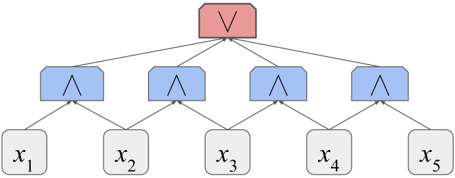
Figure 1: A circuit that takes a string $\in\{0,1\}^{5}$ and returns whether it contains the bigram $11$.

Circuit Families

A circuit family is an ordered set of circuits $\{C_{n}\}_{n\in\mathbb{N}}$ where each circuit is identified with a particular input size $n$. We say a circuit family recognizes a formal language $\mathcal{L}\subseteq\{0,1\}^{*}$ iff, for all $w\in\mathcal{L}$,

$$C_{\left\lvert w\right\rvert}(w)=1\iff w\in\mathcal{L}.$$

Circuit Complexity

Two important notions of complexity for a circuit are its size and depth. The size of a circuit is the number of gates. The depth is the longest path from an input node to the output node. For a circuit family, both quantities can be expressed as functions of the input size $n$. A circuit complexity class is a set of formal languages that can be recognized by circuit families of a certain size, depth, and set of gates. In particular, we will discuss the classes $\mathsf{AC}^{0}$ and $\mathsf{TC}^{0}$.

Definition 7.

$\mathsf{AC}^{0}$ is the set of languages $\mathcal{L}\subseteq\{0,1\}^{*}$ such that there exists a circuit family recognizing $\mathcal{L}$ with unbounded arity $\{\wedge,\vee\}$ gates, $\mathrm{poly}(n)$ size, and $\mathrm{O}(1)$ depth.

Intuitively, $\mathsf{AC}^{0}$ represents the class of problems that are highly parallelizable when the computational primitives are standard logic gates. In contrast, $\mathsf{TC}^{0}$ will also represent highly parallelizable computation, but when the gates are expanded to include threshold gates. For a bitstring $x\in\{0,1\}^{*}$, define the threshold gate $\theta_{{\geq}k}(x)$ to return $1$ iff $\geq k$ bits in $x$ are $1$, and equivalently for $\leq k$. For example, $\theta_{{\geq}3}(110011)=1$.

Definition 8.

$\mathsf{TC}^{0}$ is the set of languages $\mathcal{L}\subseteq\{0,1\}^{*}$ such that there exists a circuit family recognizing $\mathcal{L}$ with unbounded arity $\{\wedge,\vee,\theta\}$ gates, $\mathrm{poly}(n)$ size, and $\mathrm{O}(1)$ depth.

It is known that $\mathsf{AC}^{0}\subset\mathsf{TC}^{0}\subseteq\mathsf{NC}^{1}$, where $\mathsf{NC}^{1}$ denotes the languages recognizable by $\mathrm{O}(\log n)$-depth circuits with bounded gate arity. Whether or not the latter containment between $\mathsf{TC}^{0}$ and $\mathsf{NC}^{1}$ is strict is an open question. Whereas parity and other basic regular languages are outside $\mathsf{AC}^{0}$ (Furst et al., 1981), $\mathsf{TC}^{0}$ properly contains parity, although it is unknown whether it contains all the regular languages. Between $\mathsf{AC}^{0}$ and $\mathsf{TC}^{0}$ lies the class $\mathsf{ACC}^{0}$ (Yao, 1990).

Uniformity

The circuit classes defined above (and which we will use in this paper) are non-uniform, meaning circuits for different input sizes are not constrained to have any relation to each other. Non-uniform circuit families can recognize some uncomputable languages, such as the language of strings $1^{k}$ such that Turing machine $k$ does not halt on the null input (cf. Arora and Barak, 2009). In contrast, the uniform variants of circuit families are constrained such that a log-space Turing machine must output a string encoding of circuit $C_{n}$ on the input string $1^{n}$, forcing any language the circuit family can recognize to be computable. For these uniform classes (which we write with a u prefix), it is known that

$$\emph{u}\mathsf{TC}^{0}\subseteq\emph{u}\mathsf{NC}^{1}\subseteq\mathsf{L}\subseteq\mathsf{P},$$

where $\mathsf{L}$ and $\mathsf{P}$ denote the conventional complexity classes of log-space and polynomial-time decision problems. Thus, it is unknown whether $\emph{u}\mathsf{TC}^{0}$ is restricted compared to general polynomial-time computation, but if we accept the common conjecture that one (if not all) of the above containments are strict, then $\emph{u}\mathsf{TC}^{0}$ forms a restricted family of problems compared to $\mathsf{P}$, which, intuitively, are more parallelizable than other problems in $\mathsf{P}$.

5 Aren’t Transformers Universal?

We now begin our analysis of saturated transformers. Hao et al. (2022) and Hahn (2020) were able to give upper bounds on the power of hard attention without imposing any constraints on the embedding, scoring, and activation functions. The same will not be the case with saturated attention: any bounds on transformers will require leveraging some properties constraining their internal functions. One property we use will be size preservation. We will first show though that size preservation is not enough on its own: deriving a nontrivial upper bound will depend on subtle assumptions about the transformer’s datatype.

With rational values and size-preserving internal functions, we will show saturated transformers can recognize any formal language, i.e., the class $\mathsf{ALL}=\{\mathcal{L}\mid\mathcal{L}\subseteq\{0,1\}^{*}\}$. Our construction resembles the universal approximation construction of Yun et al. (2020), which relies on the ability of the transformer to uniquely encode the full input string into a single value vector. After the full sequence is encoded locally into a single vector, the activation block can be used as a black box to recognize any language.

Theorem 1.

$\mathsf{AHAT}(\mathbb{Q})=\mathsf{ALL}$.

Proof.

We construct a $1$-layer rational-valued transformer with a single head to recognize every string $w$ in any formal language $\mathcal{L}\in\mathsf{ALL}$. We will omit $\ell,h$ subscripts. Let $p_{i}$ denote the $i$th prime number. The embedding layer encodes each input token according to

$$\phi(w_{i},i)=\begin{cases}1/p_{i}&\textrm{if}\;w_{i}=1\\ 0&\textrm{otherwise.}\end{cases}$$

Since $p_{i}\sim i\log i$ for large $i$ by the prime number theorem (cf. Goldstein, 1973), the number of bits needed to represent $\phi(w_{i},i)$ is

$$\leq c\log(i\log i)\leq c\log(i^{2})=2c\log i.$$

Since $i$ had size $\log i$, this implies $\phi$ is size-preserving.

Now, we define a single uniform attention head that sums across all $i$, outputting $\sum_{w_{i}=1}\frac{1}{p_{i}}$. The denominator $q$ of this sum is the product $\prod_{i=1}p_{i}$. Observe that $w_{i}=1$ if and only if $p_{i}$ divides $q$. Thus, we can define a function $f$ that extracts the input sequence $w$ from $q$ by checking whether, for each $i$, $p_{i}$ divides $q$. We let $g$ be a function recognizing $L$, and set $f=g\circ f$. The output of the transformer will now compute whether $w\in\mathcal{L}$, since $f$ outputs an encoding of the original input sequence $w$, and $g$ decides whether $w\in\mathcal{L}$. Note that any function solving a decision problem is size-preserving, hence $f\in\mathcal{P}$. ∎

Thm. 1 says that our transformer architecture parameterized with a rational datatype can recognize any formal language. But a construction of this form feels unrealistic for two reasons. First, it requires the embedding layer to implement an unconventional prime encoding scheme in the embedding layer. Second, we are using the activation layer as a black box to recognize any language—even uncomputable ones! On the other hand, the feedforward subnetworks used in practice in transformers cannot even implement all computable functions when the weights are fixed independent of the sequence length $n$. We can get around both these issues by instead restricting the datatype to floats, which is the direction we will pursue in the remaining sections.

5.1 Resource-Bounded Transformers

In § C, we develop an alternate perspective on the universality of transformers, showing that, if the embedding function is allowed to be computed in time linear in the sequence length, then the transformer’s complexity is equivalent to its activation functions’ complexity.

Theorem 2 (Informal).

If $\phi$ can be any function computable in time linear in $n$, and the scoring and activation functions can be computed in $T(m)$ time on inputs of size $m$ with $T(m)\geqslant m$, then languages recognizable by the transformer are $\mathsf{TIME}(T(m))$.

§ C contains a formal statement and proof. For example, allowing polynomial-time functions inside the transformer implies that the transformer will recognize exactly the complexity class $\mathsf{P}$. A major unrealism about this setup is the assumption that $\phi$ can be an arbitrary function computable in time linear in $n$, motivating our main results in a more constrained setting in § 8.

5.2 Discussion

We are not stating the results in this section as evidence that practical transformers are capable of universal or arbitrary polynomial computation. Rather, the unnaturalness of these constructions (specifically, the prime numbers based position encoding) motivates us to slightly constrain our model of the transformer in a realistic way: we will switch the datatype from rationals to floats, since even using only simple uniform attention, a model with rationals and unconstrained internal functions is universal. We will soon see that this realistic constraint prevents universal simulation, and in fact bounds the capacity of the saturated transformer within $\mathsf{TC}^{0}$.

6 Beyond Hard Attention, with Floats

We now move to the setting of saturated transformers over floats. Hao et al. (2022) identified that hard-attention transformers can only recognize languages within $\mathsf{AC}^{0}$. In contrast, saturated transformers over floats can recognize the “majority” language maj, which is known to lie outside $\mathsf{AC}^{0}$ (Furst et al., 1981). Pérez et al. (2019, Prop. 3.3) show how maj can be recognized by transformers. In Thm. 3, we offer a simpler construction that leverages only a single uniform attention head, as opposed to the model of transformers they were considering. Thus, this construction is achievable with saturated attention.

⬇

frac0 = aggregate(

select_all,

indicator(tokens == 0));

frac1 = aggregate(

select_all,

indicator(tokens == 1));

maj = frac1 > frac0;

Figure 2: A program recognizing maj in RASP, a programming language designed to abstract away details of transformer computation (Weiss et al., 2021). frac{0,1} measure the fraction of inputs that are $0$ or $1$. Then maj checks whether frac1 > frac0.

Theorem 3.

$\mathsf{AHAT}(\mathbb{F})\not\subseteq\mathsf{AC}^{0}$.

Proof.

Let $\#_{\sigma}(w)\in\mathbb{N}$ denote the number of $\sigma$ tokens in string $w\in\{0,1\}^{*}$. Let $\#(w)$ denote a count vector where each element corresponds to some $\sigma\in\{0,1\}$. We define maj as follows:

$$\textsc{maj}=\big{\{}w\in\{0,1\}^{+}\mid\#_{1}(w)>\#_{0}(w)\big{\}}.$$

We will construct a $1$-layer transformer with a single head to recognize maj, omitting $\ell,h$ subscripts from $s,f,x,b$. Fig. 2 gives the same construction in RASP (Weiss et al., 2021).

Let $x_{i}=\phi(w_{i},i)$ be a $1$-hot encoding of $w_{i}$. For all $i,j$, set $s(x_{i},x_{j})=1$, resulting in a single head attending everywhere:

$$b_{i}=\frac{\#(w)}{n}.$$

Finally, set $f(b_{i})$ to return whether $\#_{1}(w)/n>\#_{0}(w)/n$, which, for $n>0$, is true iff $w\in\textsc{maj}$. ∎

Notably, the construction in Thm. 3 is not just possible within our generalized transformer framework, but can also be implemented by the standard parameterization of $\phi,s$, and $f$ in real transformers (Vaswani et al., 2017). The uniform attention pattern can be implemented by setting all query and key attention parameters to $0$. Then, we can use the affine transformation that aggregates the head outputs to compute the tuple:

$$\left\langle\frac{\#_{1}(w)-\#_{0}(w)}{n},0\right\rangle.$$

This tuple is then passed through layer normalization (Ba et al., 2016), resulting in a new tuple $\langle t_{1},t_{2}\rangle$. Crucially, $t_{1}>t_{2}$ if and only if the same applies to the quantities in the original tuple. Thus, a linear classifier can decide whether $t_{1}>t_{2}$ to successfully recognize the language, as per Def. 5.

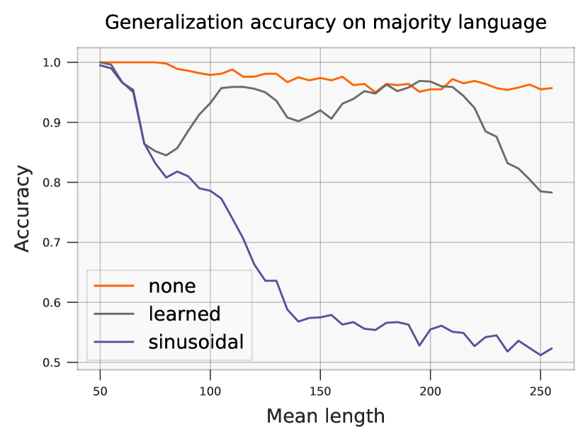
Figure 3: In practice, transformers can learn the majority language (which lies outside $\mathsf{AC}^{0}$). We train $1$-layer transformers on majority, where each line represents a different positional encoding scheme. Training string length was binomial with $n=100$. Trained models were then evaluated on generalization sets with $n$ ranging from $100$ to $500$. Mean length ($x$ axis) is $n/2$.

6.1 Empirical Validation

In Fig. 3, we show empirically that a $1$-layer transformer can learn and generalize maj. This supports our argument that the theoretical limitations of hard-attention transformers do not apply to practical transformers. We train with three different types of positional encoding: none, meaning no positional information; learned, where each position gets a trainable embedding vector, and the sinusoidal scheme of Vaswani et al. (2017). The model with no positional embeddings generalizes the best, followed by the learned embeddings. It appears that while maj is in the capacity of the transformer, the standard sinusoidal positional embedding scheme provides the wrong inductive bias for learning it. This recalls the finding of Yao et al. (2021) that the choice of positional encodings seems to greatly impact the transformer’s ability to generalize formal language tasks to longer sequences.

7 Size of Transformer Values

The theoretical limits on hard-attention transformers were derived by Hao et al. (2022) by bounding the size in bits of the representation $v_{\ell,i}$ at each layer $\ell$ and position $i$. Specifically, they show that the value $v_{\ell,i}$ is representable in $\mathrm{O}(\log n)$ bits on input sequences of length $n$. Thus, each value can only contain limited information about the input sequence, intuitively explaining their upper bound on hard-attention transformers. Inspired by their analysis, this section will show that, in a saturated transformer, each $v_{\ell,i}$ also has a size of $\mathrm{O}(\log n)$ bits. Later in § 8, we will use this property to show that saturated attention transformers are limited in the formal languages they can recognize.

7.1 Size of Float Sums

How many bits does it take to represent the value of an attention head within a saturated transformer? As a naive bound, the output of a saturated attention head is specified by a float for each of $n$ values attended over from the last layer, which would take at least linearly many bits in $n$. However, this upper bound on its size is not tight. Instead, we will show that all head and activation values can be represented in $\mathrm{O}(\log n)$ bits. Our analysis will rely heavily on the following lemma:

Lemma 1.

Let $v_{1},\cdots,v_{n}$ be a sequence of floats, each with size at most $z$. Then there exists $c$ such that $\sum_{i=1}^{n}v_{i}$ has size at most $4cz+2\log n+1$.

Proof.

Let $p_{i},q_{i}$ denote the numerator and denominator of the floating point $v_{i}$, respectively. Similarly, let $p_{s},q_{s}$ be the numerator and denominator of the float $s$. By assumption, there exists $c$ such that each $p_{i},q_{i}$ both have size $\leq cz$ for large enough $n$. We let $p_{\mathrm{max}}=\max_{i}p_{i}$ and analogously for $q_{\mathrm{max}}$. Since all $q_{i}$’s are powers of $2$, the numerator $p_{s}$ is

$$\sum_{i=1}^{n}p_{i}\cdot\frac{q_{\mathrm{max}}}{q_{i}}\leq np_{\mathrm{max}}q_{\mathrm{max}},$$

which, represented as an integer, has size:

$$\leq\log n+cz+cz=2cz+\log n.$$

On the other hand, the denominator $q_{s}=q_{\mathrm{max}}$, which has size $\leq z$. Therefore, the float representing the sum has size

$$\leq 1+2\max(2cz+\log n,z)$$

$$=4cz+2\log n+1,$$

which completes the proof. ∎

In particular, we will use Lem. 1 to show that, when each of a sequence of $n$ values has size $\mathrm{O}(\log n)$, the sum will also have size $\mathrm{O}(\log n)$.

7.2 Size of Transformer Values

We will now leverage Lem. 1 to show that the values are of bounded size in any transformer over floats with an elementwise-size-preserving attention function.

Definition 9.

A function $\alpha:\mathbb{D}^{n}\to\mathbb{D}^{n}$ is elementwise-size-preserving if, for $1\leq i\leq n$, the function $x_{i}\mapsto\alpha(x)_{i}$ is size-preserving (where $x\in\mathbb{D}^{n}$).

Note that saturated attention satisfies this definition. We are ready to prove a theorem bounding the size of the representations in transformers with elementwise-size-preserving attention.

Theorem 4.

For any transformer over $\mathbb{F}$ with $\phi,s_{\ell,h},f_{\ell}\in\mathcal{P}$ and $\alpha$ elementwise-size-preserving, for all $\ell\leq L$ and $i\leq n$, $v_{\ell,i}$ has size $\mathrm{O}(\log n)$.

Proof.

By induction over $\ell$. The proof follows the definition of transformer computation in § 3.2.

Base Case

$w_{i}\in\Sigma$ has size $\mathrm{O}(1)$, and $i\in[n]$ has size $\mathrm{O}(\log n)$. Since $\phi\in\mathcal{P}$, $v_{0,i}=\phi(w_{i},i)$ has size $\mathrm{O}(\log n)$ for all $i$.

Inductive Case

Assume $v_{\ell,i}$ has size $\mathrm{O}(\log n)$. Since $s_{\ell+1,h}\in\mathcal{P}$, $a_{\ell+1,h,i,j}=s_{\ell+1,h}(v_{\ell,i},v_{\ell,j})$ has size $\mathrm{O}(\log n)$ for all $i,j$. Since $\alpha$ is elementwise-size-preserving, we can conclude that $\alpha(a_{\ell+1,h,i,:})_{j}$ also has size $\mathrm{O}(\log n)$ for all $h,i,j$. Multiplying two floats is size-preserving (cf. § B), so $\alpha(a_{\ell+1,h,i,:})_{j}\cdot v_{\ell,j}$ has size $\mathrm{O}(\log n)$ for all $h,i,j$. We then apply Lem. 1 to conclude that $b_{\ell+1,h,i}$ has size $\mathrm{O}(\log n)$, where, recall,

$$b_{\ell+1,h,i}=\sum_{j=1}^{n}\alpha(a_{\ell,h,i,:})_{j}\cdot v_{\ell,j}.$$

Finally, computing $v_{\ell+1,i}=f_{\ell+1}(v_{\ell,i},b_{\ell,:,i})$, we conclude that $v_{\ell+1,i}$ has size $\mathrm{O}(\log n)$ for all $i$ by size preservation. ∎

Corollary 4.1.

For any saturated transformer over $\mathbb{F}$ with size-preserving internal functions, for all $\ell\leq L$ and $i\leq n$, $v_{\ell,i}$ has size $\mathrm{O}(\log n)$.

Cor. 4.1 follows because saturated attention is elementwise-size-preserving. Softmax attention, on the other hand, is not guaranteed to fulfill this property, since it requires computing the exponential function. This technical challenge prevents generalizing our technique to soft attention.

7.3 Discussion

Similar to hard-attention transformers (Hao et al., 2022), the size of each vector representation in a saturated transformer over floats is $\mathrm{O}(\log n)$. This is enough memory for individual vectors to “count”, a behavior that has been observed in both LSTMs (Weiss et al., 2018) and transformers (Bhattamishra et al., 2020). On the other hand, $\mathrm{O}(\log n)$ space is not enough memory for individual vectors (for example, the CLS output) to encode arbitrarily large combinatorial objects like trees. However, transformers are not limited to computing in an “online” fashion where tokens are consumed sequentially, meaning their effective state is $n$ values of size $\mathrm{O}(\log n)$. Notably, trees with $n$ leaves can be encoded in a distributed fashion across $n$ values of size $\mathrm{O}(\log n)$. One construction for this is, at index $i$, to store $w_{i}$ and $i$, along with a pointer $j$ to the parent. Since $i,j$ can both be represented in $\log n$ bits, each vector uses only $\mathrm{O}(\log n)$ bits.

Additionally, the $\mathrm{O}(\log n)$ space bound has implications from the perspective of circuit complexity. While saturated attention cannot be simulated in $\mathsf{AC}^{0}$, we will show in § 8 that saturated transformers over $\mathbb{F}$ can be simulated by $\mathsf{TC}^{0}$ circuits.

8 Threshold Circuit Simulation

We have proved that each value vector in a saturated transformer over floats has $\mathrm{O}(\log n)$ size. Now, we show how this implies saturated transformers can be simulated by $\mathsf{TC}^{0}$ circuits. Our results heavily leverage the following lemmas:

Lemma 2 (Hao et al. 2022).

Any function $f:\{0,1\}^{c}\to\{0,1\}^{d}$ can be computed by a boolean circuit of depth $3$ and size at most $(2^{c}+c+1)d$.

So that our results are self-contained, we reproduce a proof of this lemma in § D. Applying Lem. 2 to a size-preserving function with at most $c\log n$ input bits immediately yields:

Corollary 2.1.

Any size-preserving function with at most $c\log n$ input bits can be computed by a boolean circuit of depth $3$ and polynomial size.

In other words, such functions can be computed with $\mathsf{AC}^{0}$ circuits. In addition, we will show that the sum of $n$ floats of size at most $c\log n$ can be computed by $\mathsf{TC}^{0}$ circuits.

Lemma 3.

Let $v_{1},\cdots,v_{n}$ be a sequence of floats, each with size at most $c\log n$ for some $c$. Then the sum $\sum_{i=1}^{n}v_{i}$ is computable by a threshold circuit of constant depth and polynomial size.

Proof.

Let the integers $p_{i},q_{i}$ be the numerator and denominator of $v_{i}$. We first compute $q_{\mathrm{max}}$, the maximum $q_{i}$, using an $\mathsf{AC}^{0}$ circuit that compares all pairs $q_{i},q_{j}$, and returns the first $q_{i}$ such that $q_{j}\geq q_{j}$ for all $j$. We then use the fact that multiplication and right shift ($q_{i}$ is a power of $2$) are in $\mathsf{TC}^{0}$, in order to compute

$$r_{i}=p_{i}\frac{q_{\mathrm{max}}}{q_{i}}$$

in parallel for all $i$. Note that $q_{\mathrm{max}}$ and $q_{i}$ are both powers of $2$, so the division will be exact. Next, we leverage the fact that the sum of $n$ integers of size $\mathrm{O}(\log n)$ is in $\mathsf{TC}^{0}$ (Kayal, 2015), in order to compute the numerator of the sum $p^{\prime}=\sum_{i}r_{i}$. We select the denominator as $q^{\prime}=q_{\mathrm{max}}$. Finally, we can add an $\mathsf{AC}^{0}$ circuit that “reduces” the fraction by removing shared trailing zeros from $p^{\prime},q^{\prime}$, which is possible by 2.1. Thus, we have constructed a $\mathsf{TC}^{0}$ circuit to compute the sum of $n$ floats with size $\mathrm{O}(\log n)$. ∎

We now construct a $\mathsf{TC}^{0}$ circuit that simulates a saturated transformer over floats.

Theorem 5.

$\mathsf{AHAT}(\mathbb{F})\subseteq\mathsf{TC}^{0}$.

Proof.

For each $n$, we construct a $\mathsf{TC}^{0}$ circuit that simulates a saturated transformer on inputs of size $n$. We construct the circuit modularly, with one subcircuit for the attention mechanism, and another for the feedforward subnetwork.

Attention Head

Fix a single head in some layer. We will construct a $\mathsf{TC}^{0}$ subcircuit that simulates the attention mechanism at position $i$. The head attends over vectors $v_{1},\cdots,v_{n}$. For all $j$, $v_{j}$ has size $\mathrm{O}(\log n)$ by Thm. 4. In parallel for each $j$, we compute the scores $a_{i,j}=s(v_{i},v_{j})$ with an $\mathsf{AC}^{0}$ circuit by 2.1. We then compute $a_{i,\mathrm{max}}\triangleq\max_{j}a_{i,j}$ with an $\mathsf{AC}^{0}$ circuit by comparing all $v_{j}$ pairwise, and selecting the first $v_{k}$ such that $v_{k}\geq v_{j}$ for all $j$. We then compute “masked” values $u_{i,j}$ for each $j$ via an $\mathsf{AC}^{0}$ circuit by Lem. 2:

$$u_{i,j}\triangleq\begin{cases}v_{j}&\textrm{if}\;a_{i,j}\geq a_{i,\mathrm{max}}\\ 0&\textrm{otherwise.}\end{cases}$$

We then compute the sum $s_{i}\triangleq\sum_{j=1}^{n}u_{i,j}$ by Lem. 3. By Lem. 1, $s_{i}$ has size $\mathrm{O}(\log n)$. Now, we similarly define

$$z_{i,j}\triangleq\begin{cases}1&\textrm{if}\;a_{i,j}\geq a_{i,\mathrm{max}}\\ 0&\textrm{otherwise.}\end{cases}$$

Using an analogous sum construction with $z_{i,j}$ instead of $u_{i,j}$, we can use a $\mathsf{TC}^{0}$ circuit to compute $\left\lvert\mathcal{M}(a)\right\rvert$: the number of $j$ such that $a_{i,j}\geq a_{i,\mathrm{max}}$. Finally, since dividing floats is in $\mathsf{TC}^{0}$ (cf. § A), we can compute the head output as $s_{i}/\left\lvert\mathcal{M}(a)\right\rvert$, which has size $\mathrm{O}(\log n)$ by size preservation of division.

Feedforward

As input, $f$ receives $v_{i}$ as well as $H$ head outputs, all of which have size $\mathrm{O}(\log n)$. As the total size of the input is $\mathrm{O}(\log n)$, we can use 2.1 to compute the output of $f$ with an $\mathsf{AC}^{0}$ circuit. The size of the output is $\mathrm{O}(\log n)$ by size preservation of $f$. The same idea holds for $\phi$ as well as the linear classification head.

We have simulated each transformer component with a $\mathsf{TC}^{0}$ subcircuit, completing the proof. ∎

8.1 Discussion

Recall that, over rationals, we found that size-preserving saturated transformers could recognize any language. In contrast, we have now shown that using floating-point representations places such transformers within $\mathsf{TC}^{0}$. In this paper, we have only considered non-uniform $\mathsf{AC}^{0}$ and $\mathsf{TC}^{0}$, as opposed to the uniform variants of these classes, which are more closely connected to familiar formal language classes like the regular and context-free languages (cf. Cojocaru, 2016; Mahajan, 2007). As transformers satisfy some intuitive notion of uniformity, an open question is whether saturated transformers also fall into uniform $\mathsf{TC}^{0}$.

9 Conclusion

Compared to hard attention, saturated attention adds theoretical power to transformers. We showed that saturated attention lets transformers recognize languages outside $\mathsf{AC}^{0}$, which is the upper bound with hard attention. Further, while saturated transformers with rational values and size-preserving internal functions can recognize any language, we characterize the limits of size-preserving saturated transformers with floats. Specifically, saturated transformers with float values fall in $\mathsf{TC}^{0}$, a more powerful circuit class than $\mathsf{AC}^{0}$. Thus, going from hard to saturated attention can be understood as augmenting the model with threshold gates. This illustrates one way that the circuit complexity paradigm characterizes the power of transformers. Going forward, there are many interesting open questions that circuit analysis can answer, such as comparing the power of saturated and soft attention, and refining existing upper bounds for transformers in terms of uniform circuit families.

Appendix A Float Division

Let $/$ be truncated division between integers. We divide a float by an integer $p$ by defining an approximate multiplicative inverse $p^{-1}$. The numerator is $2^{\left\lvert p\right\rvert}/p$ and the denominator is $2^{\left\lvert p\right\rvert}$. For division by a float $p,q$, we simply apply the integer approach and then multiply by $q$. This yields numerator $2^{\left\lvert p\right\rvert}/p\cdot q$ and denominator $2^{\left\lvert p\right\rvert}$.

The fact that float division is defined in terms of integer multiplication and division implies it is size-preserving and can be simulated in $\mathsf{TC}^{0}$, which we use in § 8.

Appendix B Justifying Size Preservation

We justify that feedforward neural networks are size-preserving over floats. Feedforward neural networks are made up of a fixed (with respect to $n$) number of addition, multiplication, division, ReLU, and square root (for layer norm) operations. Therefore, it suffices to show that these operations are all in $\mathcal{S}(\mathbb{F})$.

For addition, the numerator is

$$\leq p_{1}q_{2}+p_{2}q_{1}\leq 2p_{\mathrm{max}}q_{\mathrm{max}},$$

which has size $\leq\log 2+\left\lvert p_{\mathrm{max}}\right\rvert+\left\lvert q_{\mathrm{max}}\right\rvert\leq 2(\left\lvert p_{\mathrm{max}}\right\rvert+\left\lvert q_{\mathrm{max}}\right\rvert)$ for large enough input size.

For multiplication, the numerator is just $p_{1}\cdot p_{2}$, which has size $\leq 2\left\lvert p_{\mathrm{max}}\right\rvert$. Let the denominators be $q_{1}=2^{k_{1}}$ and $q_{2}=2^{k_{2}}$. Then the denominator is $2^{k_{1}+k_{2}}$, which has size $\leq 2\left\lvert q_{\mathrm{max}}\right\rvert$.

Division can be analyzed in terms of the approximate multiplicative inverse (§ A). Its numerator has size $\leq\left\lvert p\right\rvert+1+\left\lvert q\right\rvert\leq 2(\left\lvert p\right\rvert+\left\lvert q\right\rvert)$ for large enough input size. The denominator has size $\leq\left\lvert p\right\rvert+1\leq 2\left\lvert p\right\rvert$ for large enough input size.

Size preservation is trivially satisfied for ReLU, which cannot expand the size of the input.

To make layer norm work, we just need to analyze square root, which we will define in a truncated fashion over integers. The square root of a rational, then, simple takes the square root of $p$ and $q$. We have that $\left\lvert\sqrt{p}\right\rvert\leq\left\lvert p\right\rvert$ and analogously for $q$.

Appendix C Resource-Bounded Transformers

Size preservation is one way to characterize the constraints on transformers’ internal functions; a slightly different perspective is to fix $\phi$ and analyze how the language recognition abilities of the transformer change depending on the computational resources allotted to each $s_{\ell,h}$ and $f_{\ell}$. In this section, we derive an alternate universality theorem in terms of time complexity classes. We will show that as long as $\phi$ is powerful enough, such transformers have equivalent time complexity to their activation functions.

Recall that a transformer is a tuple $\langle\Sigma,\mathbb{D},\alpha,L,H,\phi,s_{\ell,h},f_{\ell}\rangle$. In contrast to $\mathsf{AHAT}(\mathbb{D})$ (cf. Def. 6), we will now work with a different class of transformer languages $\mathsf{AHAT}(\mathbb{D},T(m))$ We will allow the embedding functions to be linear in the sequence length, and explore the effect of varying the complexity of the other internal functions. Let $\mathsf{FTIME}(T(m))$ be the set of functions computable by a Turing machine in $T(m)$ time.

Definition 10.

Let $\mathsf{AHAT}(\mathbb{D},T(n))$ be the class of languages $\mathcal{L}\subseteq\Sigma^{*}$ such that there exists a transformer $\langle\Sigma,\mathbb{D},\alpha,L,H,\phi,s_{\ell,h},f_{\ell}\rangle$ that recognizes $\mathcal{L}$, where $\phi$ runs in time linear in the sequence length $n$, and $s_{\ell,h},f_{\ell}\in\textsf{FTIME}(T(m))$.

For any $T(m)\geqslant m$, we will show transformers $\mathsf{AHAT}(\mathbb{D},T(m))$ have the complexity of their activation functions. Formally:

Theorem 2   (Formal version of Thm. 2)

For $\mathbb{D}\in\{\mathbb{F},\mathbb{Q}\}$ and $T(m)\geqslant m$,

$$\mathsf{AHAT}(\mathbb{D},T(m))\subseteq\mathsf{TIME}(T(m)).$$

Proof.

First, observe that $\mathsf{AHAT}(\mathbb{D},T(m))\subseteq\mathsf{TIME}(T(m))$, since the embedding function and saturated attention can be computed in time linear in the input sequence length, and the other internal functions can be computed in $\mathsf{FTIME}(T(m))$ by construction.

We now show $\mathsf{TIME}(m)\subseteq\mathsf{AHAT}(\mathbb{D},T(m))$. We adopt a $1$-layer transformer construction, and thus omit $\ell,h$ subscripts.We define three components of the embedding function $\phi:\Sigma\times\mathbb{N}\to\mathbb{D}^{3}$:

$$\phi(w_{i},i)_{1} =\begin{cases}2^{i-1}&\textrm{if}\;w_{i}=1\\ 0&\textrm{otherwise}\end{cases}$$

$$\phi(w_{i},i)_{2} =i$$

$$\phi(w_{i},i)_{3} =2^{\left\lvert i\right\rvert}.$$

Each of these components is computable in time linear in $n$. Define three heads $b_{1,i}$, $b_{2,i}$, $b_{3,i}$. Without loss of generality, consider $b_{h,i}$ to act on $\phi(w_{i},i)_{h}$ alone, rather than the full embeding vector. $b_{1,i}$ is defined as a uniform head, while $b_{2,i}$ and $b_{3,i}$ are computed with $s_{h}(v_{i},v_{j})=v_{j}$. Thus,

$$b_{1,i} =\frac{1}{n}\sum_{w_{j}=1}2^{j-1}$$

$$b_{2,i} =n$$

$$b_{3,i} =2^{\left\lvert n\right\rvert}.$$

Finally, we discuss how to set $f$ to compute whether $w\in\mathcal{L}$. Let $p$ be the function that extracts the numerator of a float or rational number, which is computable in $\mathrm{O}(m)$ time on float of size $m$. Within $f$, we compute $u=p(b_{1,i})$. At this point, we proceed in two cases depending on the datatype $\mathbb{D}$:

1. Rationals: If $\mathbb{D}=\mathbb{Q}$, then $u$ is the binary string $w$. Any $\mathcal{L}\in\mathsf{TIME}(T(m))$ has an indicator function $\delta\in\mathsf{FTIME}(T(m))$, which we now apply to recognize whether $w\in\mathcal{L}$.

2. Floats: If $\mathbb{D}=\mathbb{F}$, then $u=2^{\left\lvert n\right\rvert}/n\cdot w$ as in § A. Therefore, in linear time, we compute

   $$\frac{b_{2,i}}{b_{3,i}}\cdot u=\frac{n}{2^{\left\lvert n\right\rvert}}\cdot\frac{2^{\left\lvert n\right\rvert}w}{n}=w,$$

   and feed $w$ through $\delta$ as in the $\mathbb{D}=\mathbb{Q}$ case.

So, $\mathsf{TIME}(T(m))\subseteq\mathsf{AHAT}(\mathbb{D},T(m))$. ∎

Appendix D Proof from Hao et al. (2022)

The proof for Lem. 2 largely follows the proof of a core lemma of Hao et al. (2022). We reproduce a slightly adapted version of their proof here, since their manuscript is not yet publicly available, and we wish for our paper to be self-contained.

Lemma 2

Any function $f:\{0,1\}^{c}\to\{0,1\}^{d}$ can be computed by a boolean circuit of depth $3$ and size at most $d(2^{c}+c+1)$.

Proof.

The idea of the proof is to define $d$ subcircuits of size at most $2^{c}+c+1$ that compute the $d$ output bits of $f$ in parallel. We will build a circuit that computes each output bit of $f$ according to its representation in disjunctive normal form (DNF). We define a first layer of the circuit that computes the negation of each input, which takes $c$ gates. The second layer then computes the value of each DNF term by computing a conjunction ($\wedge$ gate) over the corresponding literals or negated literals. Note that a formula of $c$ variables has at most $2^{c}$ DNF terms. Finally, the third layer of the circuit computes a disjunction ($\vee$ gate) over the values of all terms, yielding the output of $f$, and adding a single gate. In summary, we have shown how to compute each output bit with a circuit of size at most $2^{c}+c+1$, which implies the full function $f$ can be computed by a circuit of size at most $d(2^{c}+c+1)$. ∎

References

- Alishahi et al. (2020) Afra Alishahi, Yonatan Belinkov, Grzegorz Chrupała, Dieuwke Hupkes, Yuval Pinter, and Hassan Sajjad, editors. 2020. Proceedings of the Third BlackboxNLP Workshop on Analyzing and Interpreting Neural Networks for NLP. Association for Computational Linguistics, Online.
- Arora and Barak (2009) Sanjeev Arora and Boaz Barak. 2009. Computational Complexity: A Modern Approach. Cambridge University Press.
- Ba et al. (2016) Jimmy Ba, Jamie Ryan Kiros, and Geoffrey E. Hinton. 2016. Layer normalization. ArXiv, abs/1607.06450.
- Bhattamishra et al. (2020) Satwik Bhattamishra, Kabir Ahuja, and Navin Goyal. 2020. On the ability and limitations of transformers to recognize formal languages. In Proceedings of the 2020 Conference on Empirical Methods in Natural Language Processing (EMNLP), pages 7096–7116, Online. Association for Computational Linguistics.
- Cojocaru (2016) Liliana Cojocaru. 2016. Advanced Studies on the Complexity of Formal Languages. Ph.D. thesis, University of Tampere.
- Devlin et al. (2019) Jacob Devlin, Ming-Wei Chang, Kenton Lee, and Kristina Toutanova. 2019. BERT: Pre-training of deep bidirectional transformers for language understanding. In Proceedings of the 2019 Conference of the North American Chapter of the Association for Computational Linguistics: Human Language Technologies, Volume 1 (Long and Short Papers), pages 4171–4186, Minneapolis, Minnesota. Association for Computational Linguistics.
- van Emde Boas (1991) Peter van Emde Boas. 1991. Machine Models and Simulations, chapter 1. MIT Press, Cambridge, MA, USA.
- Furst et al. (1981) Merrick Furst, James B. Saxe, and Michael Sipser. 1981. Parity, circuits, and the polynomial-time hierarchy. In Proceedings of the 22nd Annual Symposium on Foundations of Computer Science, SFCS ’81, page 260–270, USA. IEEE Computer Society.
- Goldstein (1973) Larry J Goldstein. 1973. A history of the prime number theorem. The American Mathematical Monthly, 80(6):599–615.
- Hahn (2020) Michael Hahn. 2020. Theoretical limitations of self-attention in neural sequence models. Transactions of the Association for Computational Linguistics, 8:156–171.
- Hao et al. (2022) Yiding Hao, Dana Angluin, and Robert Frank. 2022. Hard attention transformers and constant depth circuits. Unpublished manuscript.
- Hewitt et al. (2020) John Hewitt, Michael Hahn, Surya Ganguli, Percy Liang, and Christopher D. Manning. 2020. RNNs can generate bounded hierarchical languages with optimal memory. In Proceedings of the 2020 Conference on Empirical Methods in Natural Language Processing (EMNLP), pages 1978–2010, Online. Association for Computational Linguistics.
- Johnson (1991) David S. Johnson. 1991. A Catalog of Complexity Classes, chapter 2. MIT Press, Cambridge, MA, USA.
- Kayal (2015) Neeraj Kayal. 2015. Lecture notes for topics in complexity theory.
- Mahajan (2007) Meena Mahajan. 2007. Polynomial size log depth circuits: Between and . Bulletin of the EATCS, 91:42–56.
- Merrill (2019) William Merrill. 2019. Sequential neural networks as automata. In Proceedings of the Workshop on Deep Learning and Formal Languages: Building Bridges, pages 1–13, Florence. Association for Computational Linguistics.
- Merrill (2021) William Merrill. 2021. Formal language theory meets modern NLP. ArXiv, abs/2102.10094.
- Merrill et al. (2021) William Merrill, Vivek Ramanujan, Yoav Goldberg, Roy Schwartz, and Noah A. Smith. 2021. Effects of parameter norm growth during transformer training: Inductive bias from gradient descent. In Proceedings of the 2021 Conference on Empirical Methods in Natural Language Processing, pages 1766–1781, Online and Punta Cana, Dominican Republic. Association for Computational Linguistics.
- Peng et al. (2018) Hao Peng, Roy Schwartz, Sam Thomson, and Noah A. Smith. 2018. Rational recurrences. In Proceedings of the 2018 Conference on Empirical Methods in Natural Language Processing, pages 1203–1214, Brussels, Belgium. Association for Computational Linguistics.
- Pérez et al. (2019) Jorge Pérez, Javier Marinković, and Pablo Barceló. 2019. On the Turing completeness of modern neural network architectures. In International Conference on Learning Representations.
- Vaswani et al. (2017) Ashish Vaswani, Noam Shazeer, Niki Parmar, Jakob Uszkoreit, Llion Jones, Aidan N Gomez, Ł ukasz Kaiser, and Illia Polosukhin. 2017. Attention is all you need. In Advances in Neural Information Processing Systems, volume 30. Curran Associates, Inc.
- Weiss et al. (2018) Gail Weiss, Yoav Goldberg, and Eran Yahav. 2018. On the practical computational power of finite precision RNNs for language recognition. In Proceedings of the 56th Annual Meeting of the Association for Computational Linguistics (Volume 2: Short Papers), pages 740–745, Melbourne, Australia. Association for Computational Linguistics.
- Weiss et al. (2021) Gail Weiss, Yoav Goldberg, and Eran Yahav. 2021. Thinking like transformers. ArXiv, abs/2106.06981.
- Yao (1990) Andrew C.-C. Yao. 1990. On ACC and threshold circuits. In Proceedings of the 31st Annual Symposium on Foundations of Computer Science, pages 619–627 vol.2.
- Yao et al. (2021) Shunyu Yao, Binghui Peng, Christos Papadimitriou, and Karthik Narasimhan. 2021. Self-attention networks can process bounded hierarchical languages. In Proceedings of the 59th Annual Meeting of the Association for Computational Linguistics and the 11th International Joint Conference on Natural Language Processing (Volume 1: Long Papers), pages 3770–3785, Online. Association for Computational Linguistics.
- Yun et al. (2020) Chulhee Yun, Srinadh Bhojanapalli, Ankit Singh Rawat, Sashank Reddi, and Sanjiv Kumar. 2020. Are transformers universal approximators of sequence-to-sequence functions? In International Conference on Learning Representations.