Trust-Region Approximation of Extreme Trajectories in Power System Dynamics

Abstract

In this work we present a novel technique, based on a trust-region optimization algorithm and second-order trajectory sensitivities, to compute the extreme trajectories of power system dynamic simulations given a bounded set that represents parametric uncertainty. We show how this method, while remaining computationally efficient compared with sampling-based techniques, overcomes the limitations of previous sensitivity-based techniques to approximate the bounds of the trajectories when the local approximation loses validity because of the nonlinearity. We present several numerical experiments that showcase the accuracy and scalability of the technique, including a demonstration on the IEEE New England test system.

I Introduction

The increase of complexity in power distribution systems is translating into uncertainty in transmission stability studies [1]. Power distribution systems are traditionally modeled as lumped loads at the transmission level; but as distribution becomes active, the models become more complex [2], and their parameters become more difficult to obtain from measurements or experiments. One must understand how much the system dynamic response can vary given the uncertainty of the system parameters. Three main types of models capture parametric uncertainty in power system dynamics.

1. When parameters vary with time with some known statistical regularity, they can be modeled as forcing stochastic processes [3, 4, 5]. An example is the load demand, whose short-term variation is observed to follow an Ornstein–-Uhlenbeck process [6]. This stochastic model turns the classical differential-algebraic equation (DAE) into a stochastic differential-algebraic equation (SDAE) that can be solved by using numerical techniques [7].

2. When parameters do not vary over time or their temporal variation is much slower than the transient response, we can represent the uncertainty by means of a probability distribution function [8, 9]. Examples are the parameters of a generator [10]. In many cases, obtaining sufficiently descriptive data to create probability distributions is not feasible, particularly when considering the parameterization of load models [11].

3. When parameters do not vary over time and their statistical properties are unknown, it is common to use a range or bounded set for the parameters [12, 13]. This uncertainty model is also named unknown-but-bounded [14]. For this type of model, it is often of interest to compute the closure of all possible trajectories or extreme trajectories. Indeed, reliability criteria often specify allowable ranges for transient performance [15, 16].

In this work we adopt the last type, and we represent uncertainty as a bounded set. We consider the problem of obtaining the extreme trajectories of the DAEs that model the power system in transient dynamics studies. While characterizing these extreme trajectories of the power system response can lead to conservative insights (i.e., the trajectory extremes might have a low probability of occurring), this type of analysis is useful for propagating parametric uncertainty in load models. Because load models are aggregated representations, obtaining statistical data of the parameters is challenging. Instead, parameter ranges are usually considered [17].

To solve this problem, one can use a Monte Carlo technique that consists of sampling from the uncertainty set until statistical convergence [10, 18]. However, while Monte Carlo sampling is general and robust since it makes no assumptions on the underlying model, its slow convergence makes it impractical for large parameter spaces. Other approaches to solve this problem are based on set-theoretic methods [19], but these often have issues scaling to large systems.

More scalable approaches to characterize uncertainty have been developed using trajectory sensitivities. As shown in [12], by constructing local approximations of the DAE solutions subject to perturbations of their parameters, one can handle uncertainty efficiently. Inspired by the use of sensitivities in power systems, more work has been done to improve the computational efficiency of the trajectory sensitivities [20]. In particular, new developments in the computation of second-order sensitivities [21] pave the way for efficient use of higher-order sensitivities in simulation codes.

The authors in [22] propose a methodology to approximate the extreme trajectories given a bounded uncertainty set. The methodology consists of constructing second-order Taylor approximations of the solutions of the DAE and then solving an optimization problem to obtain the minimum and maximum at each time step. Formulating this trajectory bounding problem as an optimization problem allows it to be solved with a semidefinite programming algorithm. Despite the computational advantages of this method, however, little attention is given to the limitations of the Taylor approximation and the pitfalls of the optimization procedure. Indeed, substituting the DAE solutions by a Taylor expansion can result in incorrect results due to the nonlinearity of the response. In these cases, the solution obtained will not correspond to a critical point of the actual DAE trajectory.

In our work we build on [22] and develop a novel algorithm based on a trust-region optimization methodology that ensures that the approximate surrogate model will be sufficiently accurate and able to effectively approximate the extreme trajectories when the Taylor expansion deviates from the actual system response. The main contributions of this paper are the following:

• We propose a novel trust region-based approach to compute the extreme trajectories in dynamic simulations. By leveraging this nonlinear optimization method, we are able to increase the accuracy of the extreme trajectory approximation with respect to prior techniques.

• We carry out our analysis using dynamic models commonly used in commercial simulation software: a detailed synchronous generator, a governor, an exciter with saturation, and a composite load formed by passive and motor load.

• We show how to appropriately derive the initial conditions for the first- and second-order sensitivity systems, which are critical for quantifying the uncertainty of the initial conditions. This information is applied to the induction motor load, which has initial conditions that depend on the uncertain parameter.

• We derive a set of formulas in matrix form to integrate the first- and second-order sensitivities using the backward Euler method.

In Section II we formulate the extreme trajectory problem mathematically, and we detail a computational solution consisting of a trust-region algorithm with a second-order expansion. In Section III we present experimental results for three scenarios: a two-bus system with passive load illustrating the basic methodology, a two-bus system with dynamic load and control devices showing the benefits of this method when nonlinearity of the response increases, and a larger 39-bus system example showing the scalability of this method. In Section IV we present our conclusions.

II Methodology

The power system dynamic equations can be abstracted into a general parameterized DAE system [23]:

$$\dot{x} =f(x,y,p,t)\,$$ (1a)

$$0 =g(x,y,p,t),$$ (1b)

where $x\in\mathbf{R}^{n}$ is the differential state vector, $y\in\mathbf{R}^{m}$ is the algebraic state vector, $p\in\mathbf{R}^{p}$ is a vector of parameters, and $t$ is the time variable. The function $f()$ generally describes time-domain elements of the system (such as generators and motors), and the function $g()$ describes the network and power balance in the frequency domain. For mathematical clarity, in this section we consider a concatenated vector $z=[x^{T};y^{T}]^{T}$ and express these equations in a succinct form using a mass matrix $M$:

$$M\dot{z} =h(z,p,t)\,,$$ (2)

where $M=(I,0;0,0)$. The vector of parameters $p$ includes system parameters such as machine inertia and load coefficients. In many cases, knowledge of $p$ is not exact, and it might come in the form of either a range or a probability distribution function. Often, one would ask the following question: What would be the extreme trajectories of a certain dynamic quantity of interest, given that $p$ can take some predefined range of values?

Given the nonlinear, discontinuous nature of the power system model, this question has no straightforward answer. Mathematically, finding the extreme upper trajectory amounts to finding the argument of

$$\underset{p}{\text{maximize}} {z}_{i}(p,t)$$ (3)

subject to $$p\in\Theta,$$

for $t\in(t_{0},t_{N})$. Equivalently, the extreme lower trajectory is found by minimization. Here, $\Theta=\{p\mid\theta_{\textit{min}}\leq p\leq\theta_{\textit{max}}\}$, and $z_{i}$ is a component of the state trajectory of the system. In general we cannot find closed solutions to the power system dynamic equations; hence, we need to either sample or approximate.

A common sampling approach is to use Monte Carlo techniques. Here, our model is assumed to be a black box, and $\theta$ is sampled until statistical convergence. The benefits of this technique are that it can be implemented nonintrusively on top of any existing simulation code, and it also can be easily parallelizable. On the other hand, while much research on efficient sampling methods (importance sampling, quasi–Monte Carlo, etc.) exists, as the dimension of the parameter space increases, a greater number of samples are required to find an accurate solution, thereby rendering such methods intractable for large-scale systems.

Another approach is to approximate the equations over some local region. This is accomplished with the use of derivatives, polynomial interpolation, perturbation models, and so on. For example, although an analytical expression of $z_{i}(p,t)$ might not exist, we can approximate it around a neighborhood $p_{m}$ with a Taylor expansion:

$$z_{i}(p_{m}+s,t)\approx z_{i}(p_{m},t)+s^{T}\left.\frac{\partial z_{i}}{\partial p}\right|_{(p_{m},t)}+\frac{1}{2}s^{T}\left.\frac{\partial^{2}z_{i}}{\partial p^{2}}\right|_{(p_{m},t)}s\,.$$ (4)

Here the derivatives $\frac{\partial z_{i}}{\partial p}$ and $\frac{\partial^{2}z_{i}}{\partial p^{2}}$ can be obtained by computing the first- and second-order sensitivities with respect to $p$ of the DAE (2). The first-order sensitivity can be obtained by solving the tangent linear sensitivity equations:

$${\frac{d}{dt}\left(\frac{\partial z_{i}}{\partial p}\right)=\frac{\partial f}{\partial z_{i}}\frac{\partial z_{i}}{\partial p}+\frac{\partial f}{\partial p}}.$$ (5)

For more details on the derivation of the sensitivity equations for DAE systems readers are referred to the foundational paper [24] and the recent extension to second order [21] and to [20] for details on the discrete adjoint method. In Appendix B we have included a summary of the continuous first- and second-order sensitivity equations and derived a matrix expression to integrate the equations using the backward Euler technique.

Choi et al. [22] use a local Taylor expansion as a surrogate model of $z(p,t)$ to solve (3). This is a good approach to approximating the solution, but unfortunately the solution might be inaccurate depending on the geometry of $z(p,t)$. For a certain range of the parameters, the function may exhibit nonlinear characteristics that are not well approximated by the quadratic form, and thus the calculated maximum and minimum will not be accurate. This situation is illustrated in Figure 1 showing how the Taylor expansion at the midpoint does not capture the behavior of the function at the minimum.

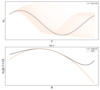
Figure 1: On the top, multiple trajectories of a dynamical system given variation of parameter $p$ are shown in orange, and the black-discontinuous curve corresponds to the midpoint trajectory. On the bottom, we slice the trajectories on a certain time step and plot the empirical function $x(t,p)$, to compare the empirical result (in black) with the second-order Taylor approximation (in orange).

Given that the trajectory functions (functions of the parameters) tend to be nonlinear and nonconvex, in our work we cast (3) as a nonlinear optimization problem, and we leverage the mature techniques in the numerical optimization field [25]. Efficient techniques to solve these types of problems include line-search-based methods and trust-region-based methods. The availability of exact second-order information allows us to select methods with better convergence properties as opposed to methods that estimate the Hessian matrix of the cost function (e.g., quasi-Newton methods). In this work we chose trust-region methods to solve the optimization problem (3). Internally, trust-region methods use second-order Taylor approximations to the solutions of the DAEs. However, the key difference from the approach in [22] is that the trust-region methods adapt the size of the trust-region based on how well the second-order Taylor series approximates the true DAE solution and will proceed iteratively until convergence. This approach aids in avoiding scenarios such as the one shown in Figure 1 where optimizing the local Taylor expansion leads to wrong results. While the trust-region approach is an efficient and robust technique, we also note that similar performance could be achieved with line-search methods.

II-A Trust-region optimization

To solve an optimization problem of a general nonlinear function $f(x)$, trust-region algorithms produce a sequence of points $\{x_{k}\}$ that converge to a point $x_{*}$, where $\nabla f(x_{*})=0$ (i.e., $x_{*}$ is a first-order critical point) by using a quadratic approximate surrogate model $m_{k}(x_{k})$ of the objective function [26]. This surrogate model is often a Taylor series expansion of $f(x)$ around $x_{k}$:

$$m_{k}(x_{k}+s)=f(x_{k})+\nabla f(x_{k})^{T}s+\frac{1}{2}s^{T}\nabla^{2}f(x_{k})s\,,$$ (6)

where $\nabla f(x_{k})$ is the gradient of the objective function, $\nabla^{2}f(x_{k})$ is the Hessian, and $s$ is a small step around $x_{k}$. The difference between $m_{k}(x_{k}+s)$ and $f(x_{k}+s)$ is small for small values of $||s||$. The optimization procedure consists of reducing $f()$ through $m_{k}()$ by seeking a step $s$ that minimizes $m_{k}$. Depending on $s$, however, the approximation error can become large enough that it will lead to incorrect results.

The trust-region algorithm ensures that, at each iteration, the approximation is valid in a suitable neighborhood $\mathcal{B}_{k}$, where

$$\mathcal{B}_{k}=\{x\in\mathbf{R}^{n}\mid\left\|x-x_{k}\right\|\leq\Delta_{k}\}\,.$$ (7)

This neighborhood is the trust region. We compute a trial step $s_{k}$ to a trial point $x_{k}+s_{k}$ that minimizes the surrogate model $m_{k}()$ and satisfies $\left\|s_{k}\right\|_{2}\leq\Delta_{k}$. If the reduction of the surrogate model is in poor agreement with the reduction of the objective function $f()$, the trial point will be rejected, and the trust region will be reduced. We check the agreement with the following ratio:

$$\rho_{k}=\frac{\textit{actual reduction}}{\textit{predicted reduction}}=\frac{f_{i}(x_{k})-f_{i}(x_{k}+s_{k})}{m_{k}(x_{k})-m_{k}(x_{k}+s_{k})}\,.$$ (8)

The following algorithm [25, Algorithm 4.1] describes the basic trust-region method. Here, $\eta_{1}$ and $\eta_{2}$ are constants, and typically they are set to $\frac{1}{4}$ and $\frac{3}{4}$, respectively [25]. We note that $\rho_{k}<0$ corresponds to the case when the model predicts a decrease in function value at $m_{k}(x_{k}+s_{k})$, but the function value, $f_{i}(x_{k}+s_{k})$, actually increased. In such scenarios, the step $s_{k}$ is rejected.

Algorithm 1 Trust Region

1:procedure Trust Region

2:     Given $\hat{\Delta}>0$, initialize $\Delta_{0}\in(0,\hat{\Delta})$, and $\eta\in\left[0,\eta_{1}\right)$

3:     for $k=0,1,2,\cdots$ do

4:         obtain $s_{k}$ by reducing $m_{k}(x)$

5:         evaluate $\rho_{k}$ from (8)

6:         if $\rho_{k}<\eta_{1}$ then

7:              $\Delta_{k+1}=\frac{1}{4}\Delta_{k}$

8:         else

9:              if $\rho_{k}>\eta_{2}$ and $\|s_{k}\|=\Delta_{k}$ then

10:                  $\Delta_{k+1}=\textrm{min}(2\Delta_{k},\hat{\Delta})$

11:              else

12:                  $\Delta_{k+1}=\frac{1}{4}\Delta_{k}$                        

13:         if $\rho_{k}>\eta$ then

14:              $x_{k+1}=x_{k}+s_{k}$

15:         else

16:              $x_{k+1}=x_{k}$               

If the step is accepted, we create a new surrogate model $m_{k+1}$ by evaluating the gradient and Hessian at $x_{k+1}$.

Usually, the most expensive step in the trust-region algorithm is solving the subproblem (that is, reducing (9)). For more details about the various strategies to solve the subproblem and convergence results, we refer the reader to [25]. Note that the Hessian can be indefinite. In this work we use a subproblem solver from [27] that uses a variant of the Steihaug–Toint method [28] with provisions for such cases.

II-B Approximation of extreme trajectories

To approximate the extreme trajectories, we use the trust-region approach to solve (3). In our case the objective function is a trajectory of the state variable at some time $t$ depending on a set of parameters $p$: $z^{t}_{i}(p)$, whereas the subproblem solved in the $k$th iteration can be written as follows (we omit the time superscript $t$ for brevity):

$$\displaystyle\underset{d}{\textrm{min}}\quad m_{k}(p_{k}+s)=z_{i}+u_{i}^{T}s+\frac{1}{2}s^{T}V_{i}s\,,\quad\textrm{s.t }\|s\|\leq\Delta_{k}\,,$$ (9)

where $m_{k}(x)$ is a surrogate based on a local quadratic approximation of the trajectory $z_{i}$ at $p$ and where $u_{i}$ and $V_{i}$ are respectively the first-order and second-order sensitivities of the $i$th state variable evaluated at $p$, as described in Appendix -B. Given the DAE system (1) over a time interval $t\in(t_{0},t_{\textit{end}})$, we discretize the interval into $j$ subintervals. Thus, the solution of (3) involves the solution of $j$ trust-region problems. For each time step $t_{j}$ the sketch of the computational procedure is as follows.

• Choose a point on the parameter interval: $p_{\textit{nom}}\in\Theta$. By default, we chose $p_{\textit{nom}}=p_{m}+\frac{p_{M}-p_{m}}{2}$.

• Integrate the DAE (1) and its sensitivity equations from $t_{0}$ to $t_{j}$. With the results we can evaluate the surrogate model defined in (9).

• Proceed with Algorithm 1, and solve the subproblem. If it is necessary to evaluate another point $p_{k}$, this will involve another integration of the DAE and its sensitivities from $t_{0}$ to $t_{j}$.

This method will require repeated integration of the DAE system and can become more computationally expensive as $j$ increases. However, one can improve this situation. For instance, an initial integration of the DAE and sensitivities with respect to $p_{\textit{nom}}$ can be done from $t_{0}$ to $t_{\textit{end}}$ and will serve as the initialization for the subproblem of the $k$ trust-region problems. Additional integrations will be carried out only if a trust-region problem requires an additional evaluation of the surrogate model. Furthermore, these extra computations can be performed in parallel. Figure 2 shows the iterative process.

Figure 2: Flowchart of the trust region. This represents the solution of a problem for a particular time point $t$. We start $p_{0}=p_{\textit{nom}}$, and for each new $p_{k}$ we need to compute the sensitivities at the new point.

We have introduced this method as an approximation of extreme trajectories. While our method would avoid situations like in Fig. 1 where the second-order Taylor model does not effectively capture the geometry of the function over the parameter variation range, we could as well fall into a local minimum or maximum that would not correspond with an extreme trajectory point. We have tested our method with detailed dynamic models and with fault scenarios of wide magnitude ranges, and we have observed that the functions of the trajectories with respect to the parameters, while nonconvex, do not seem to have multiple local minima.

In the next section we show experimentally that our method (a) improves the accuracy of [22] when the system is stressed and exhibits acute nonlinear response and (b) approximates effectively the extreme trajectories, which we verify by comparing our results with sampling techniques.

III Case studies

One of the major sources of uncertainty in power systems is the composition of the load. Since in normal scenarios the mixture of load is not known with precision, we wish to understand how system trajectories under a disturbance vary with the change of the mixture combination [13]. In other words, we would like to know how sensitive the system is to a variation of the load mixture in a set of buses. In most transient dynamic simulators, the load is modeled as a current or power injection into the system—a Thevenin equivalent. For a certain bus the active and reactive power injections can be written as

$$P_{\textit{inj}}(t) =P_{1}(t)+P_{2}(t)+\dots+P_{n}(t)\,,$$ (10)

$$Q_{\textit{inj}}(t) =Q_{1}(t)+Q_{2}(t)+\dots+Q_{n}(t)\,,$$ (11)

where each $(P_{i},Q_{i})$ represents a distinct type of load. An example is the ZIP load model, where the individual power injections are passive functions of the voltage, and the composite load model, where the individual power injections have also dynamic load models such as the ones representing induction motor models and solar inverters. In this section we obtain approximations to the extreme trajectories of generator states given perturbations of the components of the load mixture.

III-A Two-bus system with passive load

As a first example we consider the load to be a mixture of constant impedance and constant power loads (a subset of the ZIP load model):

$$P^{i}_{\textit{inj}}=P_{\textit{z}}+P_{\textit{p}}\,.$$ (12)

From the net load, $P^{i}_{\textit{inj}}$, a fraction, $\alpha$, will correspond to the constant impedance load and the rest of it, $1-\alpha$, to the constant power load. A typical way to do this is by feeder usage statistics, which can be imprecise [2]. To include this information in a dynamic simulation, we can write the constant impedance load as

$$P^{i}_{\textit{inj}}=\alpha\left(\frac{V_{i}}{V_{0}}\right)^{2}P_{0}+(1-\alpha)P_{0}\,.$$ (13)

We simulate a two-bus system consisting of a GENROU generator model connected to this load. We would like to obtain the extreme trajectories of the states of this system after a $0.6$ p.u. fault applied at $t=0.1$ sec and removed at $t=0.2$ sec, given that $\alpha\in[0.2,0.5]$. Figure 3 shows the computed extreme trajectories for the voltage magnitude of the load bus. While the effect of the parameter $\alpha$ on the variation of the voltage is notable, its relationship is quasilinear and can be represented effectively with the quadratic model (9). This is not always the case, however; in Fig. 4 we can see a similar plot of the generator frequency deviation for a segment of time after the fault. While the frequency variation is less conspicuous compared with the voltage variation, the frequency function $\omega(t,\alpha)$ exhibits more nonlinearity, which results in additional iterations. This can be seen in Fig. 5, where the initial surrogate model requires up to three iterations to approximate the function accurately.

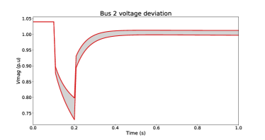
Figure 3: In red, the extreme trajectories of the voltage magnitude at bus 2 computed with the trust-region method. In grey, trajectories obtained from sampling the interval of $\alpha$ using a grid with $100$ points.

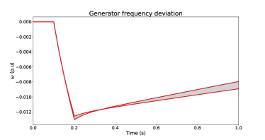
Figure 4: In red, the extreme trajectories of the generator frequency deviation computed with the trust-region method. In grey, trajectories obtained from sampling the interval of $\alpha$ using a grid with $100$ points.

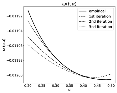
Figure 5: The continuous curve is a plot of the empirical function $\omega(t,\alpha)$ at $t=0.288$ s using Monte Carlo sampling. The dashed lines show the quadratic approximation at different iterations of the trust-region algorithm. We can see how the last iteration closely matches the minimum of the function.

By taking a slice of the frequency trajectories ensemble at time $t=0.288$ s, we can observe how the trust-region algorithm works. To find the minimum, we first build a surrogate model around the nominal point $\alpha_{1}=0.35$, and we solve the subproblem that finds a new trial step of the quadratic at $\alpha_{2}=0.364$. In this new point we compute again the function value and sensitivities and verify that $\rho>0.75$, which allow us to accept the step and check that the gradient is still above tolerance. A new trial step with the new model at $\alpha_{s}$ gives us a trial step of $\alpha_{3}=0.4792$ where we find a critical point.

We can define a simple metric to evaluate the accuracy of our method by computing the relative norm of the difference between the minimum computed with Monte Carlo sampling and the trust-region method:

$$\epsilon_{M} =\frac{\left\|M_{\textit{mc}}-M_{\textit{trust}}\right\|}{\left\|M_{\textit{mc}}\right\|}\,,$$ (14a)

$$\epsilon_{m} =\frac{\left\|m_{\textit{mc}}-m_{\textit{trust}}\right\|}{\left\|m_{\textit{mc}}\right\|}\,.$$ (14b)

The results for this example are given in I, where we find good agreement with the sampling-based method.

TABLE I: Case A: approximation relative errors

Variable	$\epsilon_{M}$	$\epsilon_{m}$
$V_{\textit{mag}}$	5.736e-09	1.320e-09
$\omega$	5.049e-04	4.171e-07

III-B Two-bus system with passive and motor load

We can modify the previous example to include an induction motor model instead:

$$P_{\textit{inj}}(V_{0},t_{0}) =\alpha P_{\textit{z}}+(1-\alpha)P_{\textit{mot}}\,,$$ (15)

$$Q_{\textit{inj}}(V_{0},t_{0}) =\alpha Q_{\textit{z}}+(1-\alpha)Q_{\textit{mot}}\,.$$ (16)

The motor equations are

$$\dot{e^{\prime}_{d}} =-\frac{1}{T_{p}}(e^{\prime}_{d}+(x_{0}-x^{\prime})i_{q})+s\omega_{s}e^{\prime}_{q}\,,$$ (17a)

$$\dot{e^{\prime}_{q}} =-\frac{1}{T_{p}}(e^{\prime}_{q}-(x_{0}-x^{\prime})i_{d})-s\omega_{s}e^{\prime}_{d}\,,$$ (17b)

$$\dot{s} =\frac{1}{2H}(\tau_{m}-e^{\prime}_{d}i_{d}-e^{\prime}_{q}i_{q})\,,$$ (17c)

$$0 =r_{a}i_{d}-x^{\prime}i_{q}+e^{\prime}_{d}+Vsin(\theta)\,,$$ (17d)

$$0 =r_{a}i_{q}-x^{\prime}i_{d}+e^{\prime}_{q}-Vcos(\theta)\,,$$ (17e)

where $x=\begin{bmatrix}e^{\prime}_{d}&e^{\prime}_{q}&s\end{bmatrix}^{T}$ and $y=\begin{bmatrix}i_{d}&i_{q}\end{bmatrix}^{T}$ are the state and algebraic variables for the DAE system, respectively. The torque value $\tau_{m}$ is to be found. The active power and reactive power consumed by the motor are written as

$$P_{\textit{mot}} =-Vsin(\theta)i_{d}+Vcos(\theta)i_{q}\,,$$ (18a)

$$Q_{\textit{mot}} =Vcos(\theta)i_{d}+Vsin(\theta)i_{q}\,.$$ (18b)

We initialize the motor with $V_{0},\theta_{0}$ and $(1-\alpha)P_{\textit{inj}}$ from a power flow solution and obtain a set of initial states $z_{0}=\begin{bmatrix}e^{\prime}_{d}&e^{\prime}_{q}&s&i_{d}&i_{q}&\tau_{m}\end{bmatrix}^{T}$. After setting the initial states (and parameter $\tau_{m}$), the motor reactive power consumption, in general, does not match $(1-\alpha Q_{0})$. To fix this discrepancy, we introduce a shunt reactance:

$$y_{\textit{sh}}=\frac{V_{0}cos(\theta_{0})i_{d}+V_{0}sin(\theta_{0})i_{q}-\alpha Q_{0}}{(V_{0})^{2}}.$$ (19)

Computing the sensitivities with respect to $\alpha$ in the case where a motor is one of the components of the load presents additional complications. In this case, the initial states and parameters $\tau,y_{\textit{sh}}$ from the motor are all dependent on $\alpha$. Hence, we need to obtain the sensitivities of the initial state with respect to $\alpha$ $\frac{d\dot{x}}{d\alpha}$. Writing the system equations in the form (2), we can derive the sensitivity equations with implicit differentiation:

$$u^{\alpha}=-\mathcal{J}^{-1}H_{\alpha}\,.$$ (20)

A similar derivation for the second-order sensitivities gives

$$v^{\alpha\alpha}=-\mathcal{J}^{-1}\left((I_{m}\otimes(u^{\alpha})^{T})\mathcal{H}u^{\alpha}+2H_{x\alpha}+H_{\alpha\alpha}\right)\,,$$ (21)

where $\mathcal{J}$ and $\mathcal{H}$ are the Jacobian and Hessian matrices of $\eqref{eq:ode}$, respectively. More notation details are presented in Appendixes -A and -B. For a practical implementation, we have found it more convenient to specify the static parameters $\tau,y_{\textit{sh}}$ as additional state variables and augment the original DAE with

$$\dot{\tau} =0\,,$$

$$\dot{y}_{\textit{sh}} =0\,.$$

In addition to the induction motor, we include a governor and an exciter with saturation. Their inclusion does not incur additional technical difficulties and allows us to obtain a system response richer in nonlinear features to better justify the effectiveness of the trust-region method. A $0.05$ p.u. fault is applied at bus 2 from $t=0.25$ to $t=0.40$ seconds; $\alpha$ is restricted in the range $[0.3,1.0]$.

We compare the trust-region method with the approach delineated in [22] where only the Taylor expansion at the nominal point is used. Figures  6 and 7 show that the trust-region approach can compute the extreme trajectories with higher accuracy, particularly with regard to frequency response. The trust-region minimization proceeds as follows: the surrogate model is built at the nominal point $\alpha=0.65$, resulting in the trial point $\alpha=0.3$; $\rho$ is found to be below $\frac{1}{4}$, and thus the trust radius is reduced, which leads to a new trial point at $\alpha=0.4$. This iterative process, as illustrated in Fig. 8, eventually converges to the critical point at $\alpha=0.398$. Figure 8 also shows that the initial Taylor model does not capture the curvature of the model. Quantified evaluation of the errors for the two approaches is given in Table II.

We next perform additional simulations with this same system, where we compute the relative errors for a range of fault values from $0.55$ p.u to $0.05$ p.u. As the fault resistance decreases, the disturbance is greater, which leads to a higher degree of nonlinearity. In Fig. 9 we have plotted the error of both the Taylor approach and the trust-region approach for a set of state variables. We can see that while these methods incur similar error for mild disturbances, as nonlinearity grows, the error of the trust-region method remains small.

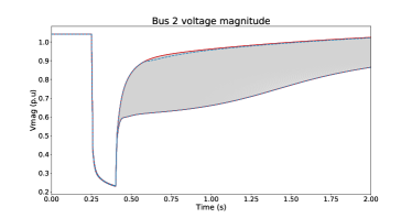
Figure 6: In red, the extreme trajectories of the voltage magnitude at bus 2 computed with the trust-region method. In grey, trajectories obtained from sampling the interval of $\alpha$ using a grid with $1,000$ points. In dashed-blue, the optimization is carried out with the model at the nominal point.

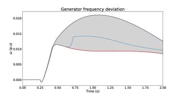
Figure 7: In red, the extreme trajectories of the generator frequency deviation computed with the trust-region method. In grey, trajectories obtained from sampling the interval of $\alpha$ using a grid with $1,000$ points. In dashed-blue, the optimization is carried out with the model at the nominal point.

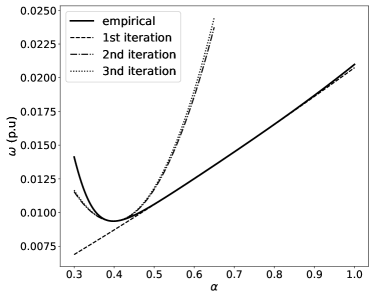
Figure 8: The continuous curve is a plot of the empirical function $\omega(t,\alpha)$ at $t=0.288$ using Monte Carlo sampling. The dashed lines show the quadratic approximation at several iterations of the trust-region algorithm.

TABLE II: Case B: approximation relative errors

Variable	$\epsilon^{\textit{Taylor}}_{M}$	$\epsilon^{\textit{Trust}}_{M}$	$\epsilon^{\textit{Taylor}}_{m}$	$\epsilon^{\textit{Trust}}_{m}$
$V_{\textit{mag}}$	4.879e-03	4.172e-09	9.116e-07	8.407e-09
$\omega$	3.991e-08	3.991e-08	0.303	1.406e-06

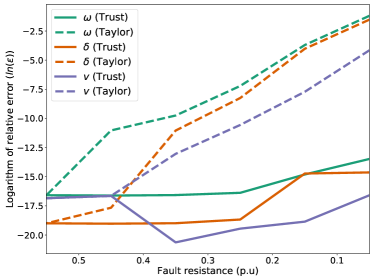
Figure 9: Logarithm of the relative error for the Taylor (dashed line) and the trust-region (continuous line) algorithms for decreasing fault resistance values. The state variables depicted are the generator speed, the generator angle, and voltage magnitude. As we decrease the resistance of the fault, the perturbation of the system is greater, leading to large nonlinearities. We can see how the error incurred by our method remains controlled.

III-C New England test system

In this last example we show the scalability of our algorithm with the New England test system (Fig. 10). Here we revert to the passive ZIP load model introduced in III-A. In the previous cases we had a single parameter, but now the dimension of the parameter space is 19 (that is, the number of loads), and computations become more expensive.

Because of the high dimensionality of the parameter space, we cannot plot the empirical function as we did in the preceding sections. In Fig. 11 we show the minimum trajectory of the frequency deviation of the generator at bus 30 given that for each load $k$ the parameter $\alpha_{i}\in[0,1]$ using our trust-region technique. We also use Monte Carlo sampling to obtain the minimum trajectory by sampling uniformly from the parameter space, and we plot the result for increasing amounts of samples.

We can see in the augmented section plot of Fig. 11 how Monte Carlo (MC) converges slowly. We observe that, despite increasing the sampling number by an order of magnitude, subsequent MC simulations approach the trust-region solution with smaller increments each time.

To verify that indeed the trust-region solution that we show in Fig. 7 is the minimum we would obtain with a sampling-based procedure, we sample around a small region near the trust-region solution. For the nadir of Fig. 11, roughly from $t=0.25$ to $t=0.42$, we observe that the trust-region algorithm finds a local minimum at one of the corners of the parameter space in which $\alpha_{i}=0$. Now we sample uniformly from the region $\alpha_{i}\in[0,1]$ and observe that the trust-region solution closely matches the MC one (see Fig. 12). Using the trust-region technique, we were able to compute this case in 2 minutes and 37 seconds using a prototype implementation in the Python programming language, whereas the computational time of MC is 17 minutes and 16 seconds for $10,000$ samples.

In some trajectories we observe that the extreme boundaries of the parameter region (the corners) correspond to extremes of the function, and this situation would motivate the use of set-theoretic techniques. However, this is not true in general—especially when acute nonlinearities and discontinuities, typical of power system dynamics under large disturbances, arise in the simulation.

Figure 10: New England test system. A three-phase to ground fault is applied at bus 2. We examine the behavior of generators 1 and 10 at buses 30 and 39, respectively.

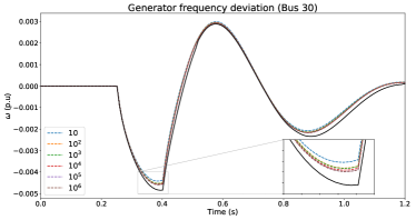
Figure 11: In black, the minimum trajectory computed with the trust-region method. Dashed lines represent the same minimum trajectory computed with Monte Carlo with increasing number of samples. We can see that Monte Carlo converges slowly.

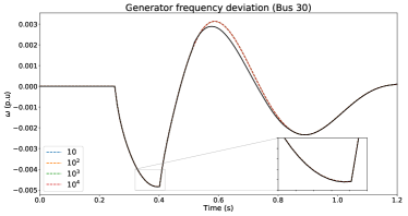
Figure 12: In black, the minimum trajectory computed with the trust-region method. Dashed lines represent the same minimum trajectory computed with Monte Carlo with increasing number of samples. This time the samples are drawn from a smaller region that we estimate to be closer to the minimum in the interval $t=0.25$ to $t=0.42$.

IV Conclusion and future work

In this work we have proposed an algorithm to compute trajectory extremes in power system dynamics using second-order sensitivities and a trust-region optimization approach. In addition to previous work where Taylor expansions were used as a surrogate of the DAE solution, our method guarantees that the local minimum computed with the sensitivities will be acceptably close to the actual DAE solution without a large increase in computational expense.

We have exemplified our technique with generator and load models used in common transient dynamics software packages (e.g., round rotor dynamic model with exciter, governor, and saturation) showing that the technique can be applied to realistic power systems. Computing the effect of load parameters on the dynamic trajectories is an important task as load models become more complex. For this purpose we have introduced a mixture model of a passive load and an induction motor and derived the first- and second-order sensitivities of the initial conditions of the motor with respect to the mixture parameter.

We have also derived a backward Euler implementation of the first- and second-order sensitivities computation, and we have detailed ways to compute these effectively.

In the future it will be of interest to extend this optimization method to models that present protection-induced discontinuities to analyze phenomena such as fault-induced delayed voltage recovery. Furthermore, describing the power system with models of prespecified nonlinearity, such as the Luŕe system formalism, could help us obtain closed-form results of higher generalization power. Our method has considerable room to be optimized such that it can be used for much larger systems. In the future we will work on efficient computation and usage of second-order sensitivities that include parallelization and randomization.

-A Differentials and Notation

Let $\mathbf{f}:S\to\mathbf{R}^{m},S\in\mathbf{R}^{n}$ be a vector function, and let z be an interior point of $S$. If we can find a matrix $\mathcal{J}\in\mathbf{R}^{m\times n}$ such that

$$f(z+d)=f(z)+\mathcal{J}d+\mathbf{O}(\|d\|^{2})\,,$$ (22)

then this function is differentiable at $z$, and the matrix $\mathcal{J}$ is the Jacobian matrix. Let us now define the Hessian matrix for a scalar function $f_{i}$. The Hessian matrix at $z$ is written $\mathcal{H}_{i}\in\mathbf{R}^{n\times n}$, where its entries are the second-order partial derivatives of $f_{i}$. For our vector function $f$, we define

$$\mathcal{H}=\begin{bmatrix}\mathcal{H}_{1}\\ \mathcal{H}_{2}\\ \vdots\\ \mathcal{H}_{m}\end{bmatrix}\in\mathbf{R}^{mn\times n}\,.$$ (23)

This allows us to write the second-degree Taylor expansion:

$$f(z+d)=f(z)+\mathcal{J}d+\frac{1}{2}(I_{m}\otimes d^{T})\mathcal{H}d+\mathbf{O}(\|d\|^{3})\,,$$ (24)

where the quadratic term is simply

$$(I_{m}\otimes d^{T})\mathcal{H}d=\begin{bmatrix}d^{T}\mathcal{H}_{1}d\\ d^{T}\mathcal{H}_{2}d\\ \vdots\\ d^{T}\mathcal{H}_{m}d\end{bmatrix}^{T}\,.$$ (25)

In our work with sensitivities we need to use partial derivatives extensively. For a function $f(x,y,p)$, where $x,y,p$ are vectors, we define $F_{x}$ to be the portion of the Jacobian matrix of $f(x,y,p)$ w.r.t. $x$, $F_{y}$ the portion of the Jacobian matrix of $f(x,y,p)$ w.r.t. $y$, and so on. We will often use the notation $F_{\alpha x}$, where $\alpha$ is an element of $p$. Because $\alpha$ is a scalar, this is equivalent to the matrix $\frac{dF_{x}}{d\alpha}$.

-B Implementation of Trajectory Sensitivities

Let us consider the DAE system (1) and elements of the parameter vector p: $\alpha\triangleq p_{i}$, $\beta\triangleq p_{j}$. The first-order sensitivity vector with respect to $\alpha$ is written

$$u^{\alpha}=\begin{bmatrix}u^{\alpha}_{x}&u^{\alpha}_{y}\end{bmatrix}=\begin{bmatrix}\frac{\partial x_{1}}{\partial\alpha},\frac{\partial x_{2}}{\partial\alpha},\dots,\frac{\partial y_{1}}{\partial\alpha},\dots\end{bmatrix}\,.$$ (26)

The continuous first-order sensitivities can be computed as follows:

$$\begin{bmatrix}\dot{u}_{x}^{\alpha}\\ 0\end{bmatrix}=\begin{bmatrix}F_{x}&F_{y}\\ G_{x}&G_{y}\end{bmatrix}\begin{bmatrix}u_{x}^{\alpha}\\ u_{y}^{\alpha}\end{bmatrix}+\begin{bmatrix}F_{\alpha}\\ G_{\alpha}\end{bmatrix}\,.$$ (27)

Equation (27) is a nonhomogeneous linear differential equation and can be integrated with a backward Euler scheme. If we set $\Delta t$ to be our time step, then we just need to solve the following linear system:

$$\begin{bmatrix}\Delta tF_{x}-I&\Delta tF_{y}\\ G_{x}&G_{y}\end{bmatrix}\begin{bmatrix}\{u_{x}^{\alpha}\}^{t}\\ \{u_{y}^{\alpha}\}^{t}\end{bmatrix}=\begin{bmatrix}-\Delta t(F_{\alpha})-\{u^{\alpha}\}^{t-1}x\\ -G_{\alpha}\end{bmatrix}\,.$$ (28)

The second-order sensitivity vector is defined as follows:

$$v^{\alpha\beta}=\begin{bmatrix}v^{\alpha\beta}_{x}&v^{\alpha\beta}_{y}\end{bmatrix}=\begin{bmatrix}\frac{\partial x_{1}}{\partial\alpha\beta},\frac{\partial x_{2}}{\partial\alpha\beta},\dots,\frac{\partial y_{1}}{\partial\alpha\beta},\dots\end{bmatrix}\,.$$ (29)

For the second-order sensitivities the structure of the equations is also a nonhomogeneous linear differential equation but has a more complex forcing term $\xi$ that depends on the first-order sensitivities:

$$\begin{bmatrix}\dot{v}_{x}^{\alpha\alpha}\\ 0\end{bmatrix}=\begin{bmatrix}F_{x}&F_{y}\\ G_{x}&G_{y}\end{bmatrix}\begin{bmatrix}v^{\alpha\alpha}_{x}\\ v^{\alpha\alpha}_{y}\end{bmatrix}+\xi(x,y,u)\,,$$ (30)

where the forcing term $\xi=\begin{bmatrix}\xi_{x}&\xi_{y}\end{bmatrix}^{T}$ is

$$\begin{bmatrix}F_{\alpha\alpha}\\ G_{\alpha\alpha}\end{bmatrix}+2\begin{bmatrix}F_{\alpha x}&F_{\alpha y}\\ G_{\alpha x}&G_{\alpha y}\end{bmatrix}\begin{bmatrix}u^{\alpha}_{x}\\ u^{\alpha}_{y}\end{bmatrix}+(I_{m}\otimes(u^{\alpha})^{T})\mathcal{H}u^{\alpha}\,.$$ (31)

Since this forcing term is given, the structure of the integration is exactly the same as before:

$$\begin{bmatrix}\Delta tF_{x}-I&\Delta t(F_{y})\\ G_{x}&G_{y}\end{bmatrix}\begin{bmatrix}\{v_{x}^{\alpha\alpha}\}^{t}\\ \{v_{y}^{\alpha\alpha}\}^{t}\end{bmatrix}=\begin{bmatrix}-\Delta t(\xi_{x})-\{v^{\alpha\alpha}_{x}\}^{t-1}\\ -\xi_{y}\end{bmatrix}\,.$$ (32)

The mixed sensitivities $v^{\alpha\beta}$ are obtained with the same equation (30) but with a different forcing term $\xi$:

$$\begin{bmatrix}F_{\alpha\beta}\\ G_{\alpha\beta}\end{bmatrix} +\begin{bmatrix}F_{\alpha x}&F_{\alpha y}\\ G_{\alpha x}&G_{\alpha y}\end{bmatrix}\begin{bmatrix}u^{\alpha}_{x}\\ u^{\alpha}_{y}\end{bmatrix}$$ (33)

$$+\begin{bmatrix}F_{\beta x}&F_{\beta y}\\ G_{\beta x}&G_{\beta y}\end{bmatrix}\begin{bmatrix}u^{\beta}_{x}\\ u^{\beta}_{y}\end{bmatrix}+(I_{m}\otimes(u^{\alpha})^{T})\mathcal{H}u^{\beta}\,.$$ (34)

We define the matrix of columns $U=\begin{bmatrix}u^{\alpha}&u^{\beta}&\dots\end{bmatrix}$, where each rows $u_{i}$ will represent the sensitivities of the $i$th variable with respect to all the parameters. At the same time we define the matrix.

$$V_{x}=\begin{bmatrix}\frac{\partial^{2}x}{\partial\alpha\alpha}&\frac{\partial^{2}x}{\partial\alpha\beta}&\dots\\ \frac{\partial^{2}x}{\partial\beta\alpha}&\frac{\partial^{2}x}{\partial\beta\beta}&\dots\\ \dots&\dots&\ddots\end{bmatrix}$$ (35)

For a system of $p$ parameters we will have $p$ $n-$dimensional vectors of first-order sensitivities, $p$ $n-$dimensional vectors of second-order self-sensitivities, and $\frac{p^{2}-p}{2}$ $n-$dimensional vectors of second-order mixed sensitivities. A priori, it might seem that the computations involved as we increase the dimension of our parameters are too onerous. However, one should note that the linear system that we solve for each sensitivity system is the same and thus one can leverage a solver with multiple right-hand sides. In any case, the polynomial nature of the growth, compared with the exponential growth required to sample the parameter space in Monte Carlo methods, makes this method much more computationally feasible.

References

- [1] G. Chaspierre, P. Panciatici, and T. V. Cutsem, “Modelling active distribution networks under uncertainty: Extracting parameter sets from randomized dynamic responses,” in 2018 Power Systems Computation Conference (PSCC), IEEE, June 2018.
- [2] “Reliability Guideline: Developing Load Model Composition Data,” tech. rep., North American Electric Reliability Corporation, March 2017.
- [3] F. Milano and R. Zarate-Minano, “A systematic method to model power systems as stochastic differential algebraic equations,” IEEE Transactions on Power Systems, vol. 28, pp. 4537–4544, Nov. 2013.
- [4] S. V. Dhople, Y. C. Chen, L. DeVille, and A. D. Dominguez-Garcia, “Analysis of Power System Dynamics Subject to Stochastic Power Injections,” IEEE Transactions on Circuits and Systems I: Regular Papers, vol. 60, pp. 3341–3353, dec 2013.
- [5] M. Adeen and F. Milano, “On the impact of auto-correlation of stochastic processes on the transient behavior of power systems,” IEEE Transactions on Power Systems, vol. 36, pp. 4832–4835, Sept. 2021.
- [6] C. Roberts, E. M. Stewart, and F. Milano, “Validation of the Ornstein–Uhlenbeck process for load modeling based on µPMU measurements,” in 2016 Power Systems Computation Conference (PSCC), pp. 1–7, IEEE, jun 2016.
- [7] Z. Y. Dong, J. H. Zhao, and D. J. Hill, “Numerical Simulation for Stochastic Transient Stability Assessment,” IEEE Transactions on Power Systems, vol. 27, pp. 1741–1749, nov 2012.
- [8] J. Hockenberry and B. Lesieutre, “Evaluation of uncertainty in dynamic simulations of power system models: The probabilistic collocation method,” IEEE Transactions on Power Systems, vol. 19, pp. 1483–1491, Aug. 2004.
- [9] Y. Xu, L. Mili, A. Sandu, M. R. von Spakovsky, and J. Zhao, “Propagating uncertainty in power system dynamic simulations using polynomial chaos,” IEEE Transactions on Power Systems, vol. 34, pp. 338–348, Jan. 2019.
- [10] J. V. Milanović, “Probabilistic stability analysis: the way forward for stability analysis of sustainable power systems,” Philosophical Transactions of the Royal Society A: Mathematical, Physical and Engineering Sciences, vol. 375, p. 20160296, July 2017.
- [11] A. Faris, D. Kosterev, J. H. Eto, and D. Chassin, “Load composition analysis in support of the NERC Load Modeling Task Force 2019–2020 field test of the composite load model,” 6 2020.
- [12] I. A. Hiskens and J. Alseddiqui, “Sensitivity, approximation, and uncertainty in power system dynamic simulation,” IEEE Transactions on Power Systems, vol. 21, no. 4, pp. 1808–1820, 2006.
- [13] J.-K. Kim, B. Lee, J. Ma, G. Verbic, S. Nam, and K. Hur, “Understanding and evaluating systemwide impacts of uncertain parameters in the dynamic load model on short-term voltage stability,” IEEE Transactions on Power Systems, pp. 1–1, 2020.
- [14] F. C. Schweppe, Uncertain dynamic systems. Prentice-Hall, hardcover ed., 1973.
- [15] B. Lesieutre, “Improving Dynamic Load and Generator Response Performance Tools,” tech. rep., LBNL, Berkeley, 2005.
- [16] NERC, “Standard TPL-001-4 — Transmission System Planning Performance Requirements.” https://www.nerc.com/files/TPL-001-4.pdf.
- [17] M. Tenza and S. Ghiocel, “An analysis of the sensitivity of WECC grid planning models to assumptions regarding the composition of loads,” Mitsubishi Electric Power Products, 2016.
- [18] K. Timko, A. Bose, and P. Anderson, “Monte Carlo simulation of power system stability,” IEEE Transactions on Power Apparatus and Systems, vol. PAS-102, pp. 3453–3459, Oct. 1983.
- [19] Y. Zhang, Y. Li, K. Tomsovic, S. M. Djouadi, and M. Yue, “Review on set-theoretic methods for safety verification and control of power system,” IET Energy Systems Integration, vol. 2, pp. 226–234, Sept. 2020.
- [20] H. Zhang, S. Abhyankar, E. Constantinescu, and M. Anitescu, “Discrete adjoint sensitivity analysis of hybrid dynamical systems with switching,” IEEE Transactions on Circuits and Systems I: Regular Papers, vol. 64, no. 5, pp. 1247–1259, 2017.
- [21] S. Geng and I. A. Hiskens, “Second-order trajectory sensitivity analysis of hybrid systems,” IEEE Transactions on Circuits and Systems I: Regular Papers, vol. 66, no. 5, pp. 1922–1934, 2019.
- [22] H. Choi, P. J. Seiler, and S. V. Dhople, “Propagating uncertainty in power-system DAE models with semidefinite programming,” IEEE Transactions on Power Systems, vol. 32, no. 4, pp. 3146–3156, 2017.
- [23] F. Milano, Power System Modelling and Scripting. Springer Berlin Heidelberg, 2010.
- [24] I. Hiskens and M. Pai, “Trajectory sensitivity analysis of hybrid systems,” IEEE Transactions on Circuits and Systems I: Fundamental Theory and Applications, vol. 47, no. 2, pp. 204–220, 2000.
- [25] J. Nocedal and S. J. Wright, Numerical Optimization. Springer Series in Operations Research and Financial Engineering, New York: Springer, 2006.
- [26] A. R. Conn, N. I. M. Gould, and P. L. Toint, Trust Region Methods. Society for Industrial and Applied Mathematics, Jan. 2000.
- [27] “Trustregion: Trust-region subproblem solver.” https://github.com/lindonroberts/trust-region.
- [28] N. I. M. Gould, S. Lucidi, M. Roma, and P. L. Toint, “Solving the trust-region subproblem using the Lanczos method,” SIAM Journal on Optimization, vol. 9, pp. 504–525, Jan. 1999.