Impact of three-nucleon forces on gravitational wave emission from neutron stars

Abstract

The detection of gravitational radiation, emitted in the aftermath of the excitation of neutron star quasi-normal modes, has the potential to provide unprecedented access to the properties of matter in the star interior, and shed new light on the dynamics of nuclear interactions at microscopic level. Of great importance, in this context, will be the sensitivity to the modelling of three-nucleon interactions, which are known to play a critical role in the high-density regime. We report the results of a calculation of the frequencies and damping times of the fundamental mode, carried out using the equation of state of Akmal, Pandharipande and Ravenhall as a baseline, and varying the strength of the isoscalar repulsive term the Urbana IX potential within a range consistent with multimessenger astrophysical observations. The results of our analysis indicate that repulsive three-nucleon interactions strongly affect the stiffness of the equation of state, which in turn determines the pattern of the gravitational radiation frequencies, largely independent of the mass of the source. The observational implications are also discussed.

Ever since their discovery, more than 50 years ago, neutron stars (NSs) have been the subject of extensive theoretical and experimental investigation, aimed at exploiting the potential of these systems as unparalleled astrophysical laboratories. The information extracted from the available data, including precise measurements of NS masses Cromartie et al. (2020) and, more recently, radii B.P. Abbott, R. Abbott, T.D. Abbott, F. Acernese, K. Ackley, C. Adams, T. Adams, P. Addesso, R.X. Adhikari, V.B. Adya et al. (2017) and tidal deformabilities Riley et al. (2019) have been effectively exploited to test the existing theoretical models.

A primary goal of NS studies is obtaining information on the Equation of State (EOS) of nuclear matter in the region of supranuclear densities, in which the microscopic dynamical models are largely unconstrained by the data collected in terrestrial laboratories. The EOS—that is, the non trivial relation linking pressure and energy density—is still largely unknown. The measured properties of atomic nuclei, supplemented by the available astrophysical observations, do not allow to unambiguously determine either the nature of the constituents of NS matter, or their interactions over the relevant range of baryon density, which extends over many orders of magnitude.

In the coming years, new insight will be made possible by the development of multi-messenger astronomy, which has already brought about impressive progress. The combination of data collected by gravitational-wave (GW) interferometers and electromagnetic (EM) observatories will provide a powerful tool to advance our understanding of the structure and dynamics of dense nuclear matter.

The detection of gravitational radiation emitted in the aftermath of the excitation of Quasi Normal Modes (QNM) may play a most important role, ushering the long anticipated era of neutron star seismology N. Andersson and K.D. Kokkotas (1998); O. Benhar, V. Ferrari, and L. Gualtieri (2004); K. Glampedakis and L. Gualtieri (2018); Andersson (2021). The measurement of the frequencies and damping times of NS oscillations, which have been shown to depend significantly on both the composition and dynamics of matter in the star interior O. Benhar, V. Ferrari, and L. Gualtieri (2004); O. Benhar, E. Berti, and V. Ferrari (1999), has the potential to provide unprecedented access not only to the nuclear matter EOS—whose density dependence is often parametrised in terms of average nuclear properties such as the compressibility module and the symmetry energy—but also to specific features of the underlying dynamics at microscopic level.

In this article, we report the results of a calculation of the frequencies and damping times of the fundamental mode, routinely referred to as $f$ mode, carried out using a set of EOS obtained within the framework of non relativistic many-body theory.

The $f$ mode is prominent amongst all possible oscillation modes, because it is a very efficient GW emitter involved in a variety of astrophysical scenarios, including isolated NS as well as inspiralling binary systems. In isolated NSs, $f$ modes can be excited in core-collapse supernovae leading to the NS formation V. Morozova. D. Radice, A. Burrows, and D. Vartanyan (2018), or in a starquake L. Keer and D.I. Jones (2015). In binaries systems, on the other hand, tidal effects include two contributions: a static response—related to the well known tidal deformability parameter $\Lambda$—during the adiabatic inspiral, and a resonance between the tidal field and the NS oscillation modes, mostly the $f$-mode G. Pratten, P. Schmidt, and T. Hinderer (2020). The emission of gravitational radiation following the excitation of the $f$ mode is also expected to occur in the merger and post-merger phases A. Bauswein and H.T. Janka (2012); K. Takami,1 L. Rezzolla, and L. Baiotti (2014). In these regimes, spacetime perturbations must be calculated with respect to a rapidly evolving background, but numerical simulations indicate the presence of high-frequency components related to the $f$ mode Stergioulas et al. (2011); Vretinaris et al. (2020). In addition, it has been shown that pre- and post-merger features can be related Chakravarti and Andersson (2020); Lioutas et al. (2021); Bernuzzi et al. (2015). The authors of Ref. Lioutas et al. (2021) have found an analytic mapping between the $f$-mode frequency of static stars and the dominant GW frequency of merger remnants, allowing to connect the masses in the two regimes.

In order to investigate the sensitivity to the description of nuclear dynamics, the Hamiltonian employed to obtain the EOS of Akmal, Pandharipande and Ravenhall (APR) Akmal et al. (1998)—widely used in neutron star applications—has been modified, changing the value of the parameter $\alpha$, determining the strength of repulsive three-nucleon interactions. These interactions are known to be largely isoscalar, and play a dominant role in the high-density region.

The present work can be seen as a complementary follow up to the pioneering study of Ref. Maselli et al. (2021), whose authors inferred a range of values of $\alpha$ using multi-messenger astrophysical data. The datasets employed in the analysis of Ref. Maselli et al. (2021) included the GW observation of the binary NS event GW170817 B.P. Abbott, R. Abbott, T.D. Abbott, F. Acernese, K. Ackley, C. Adams, T. Adams, P. Addesso, R.X. Adhikari, V.B. Adya et al. (2017), the spectroscopic observation of the millisecond pulsars PSR J0030+0451 performed by the NICER satellite Riley et al. (2019), and the high-precision measurement of the radio pulsars timing of the binary PSR J0740+6620 Cromartie et al. (2020), providing information on the maximum NS mass that must be supported by the EOS.

This article is organised as follows. The nuclear Hamiltonian employed in our study, the parametrisation of the three-nucleon potential and the main features of the corresponding EOSs of dense matter are discussed in Sect. I. In Sect. II we outline the formalism of stellar perturbation theory, employed to obtain the frequencies of QNMs, while the numerical results of our work are reported in Sect. III. Finally, In Sect. IV we summarise our findings and state the conclusions.

I Dynamics of neutron star matter

Our work is based on the description of nuclear matter as a collection of point like nucleons, whose interactions are described by the non relativistic Hamiltonian

$$H=\sum_{i}\frac{p_{i}^{2}}{2m}+\sum_{i<j}v_{ij}+\sum_{i<j<k}V_{ijk}\ ,$$ (1)

where $m$ and ${\bf p}$ denote the nucleon mass and momentum, respectively.

The nucleon-nucleon (NN) potential $v_{ij}$ is designed to account for the observed properties of the two-nucleon system, in both bound and scattering states, while inclusion of the three-nucleon (NNN) potential $V_{ijk}$—required to take into account processes involving the internal structure of the nucleons Friar (1986)—allows to reproduce the measured ground-state energy of the NNN bound state and explain saturation of isospin-symmetric matter (SNM). The predictive power of the approach based on the Hamiltonian of Eq. (1) has been firmly established by the results of calculations carried out using Quantum Monte Carlo techniques, providing an accurate description of a variety of properties of nuclei with mass number $A\leq 12$ Carlson et al. (2015).

n this study we have adopted as a baseline the Hamiltonian described in Refs. Akmal and Pandharipande (1997); Akmal et al. (1998), comprising the Argonne $v_{18}$ NN potential (AV18) Wiringa et al. (1995)—corrected to take into account relativistic boost corrections, needed to describe NN interactions in the locally inertial frame associated with a NS—and the Urbana IX NNN potential (UIX) Pudliner et al. (1995).

I.1 Parametrisation of the NNN potential

Commonly used phenomenological models of irreducible NNN interactions, such as the UIX potential, are split into two parts according to

$$V_{ijk}=V^{2\pi}_{ijk}+V^{R}_{ijk}\ .$$ (2)

In the above equation, $V^{2\pi}_{ijk}$ is the attractive Fujita-Miyiazawa potential Fujita and Miyazawa (1957), describing two-pion exchange processes in which a NN interaction leads to the excitation of a $\Delta$ resonance, while $V^{R}_{ijk}$ is a purely phenomenological repulsive potential. The Fujita-Miyiazawa mechanism is schematically illustrated in Fig. 1.

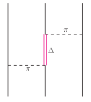
Figure 1: Diagrammatic representation of the NNN interaction described by the Fujita-Miyiazawa potential. Dashed lines depict pion-exchange, while the solid lines and the double line represent nucleons and the $\Delta$ resonance, respectively.

The strengths of $V^{2\pi}_{ijk}$ and $V^{R}_{ijk}$ are adjusted in such a way as to reproduce the binding energy of [3][]He and the empirical equilibrium density of isospin-symmetric matter (SNM), respectively. On the other hand, the NNN potential is totally unconstrained in the region of supranuclear densities, relevant to the description of NS properties, in which its contribution becomes important or even dominant.

The contributions of $V^{2\pi}_{ijk}$ and $V^{R}_{ijk}$ to the ground-state energy per nucleon of SNM and pure neutron matter (PNM), obtained from the results reported in Refs. Akmal and Pandharipande (1997); Akmal et al. (1998), are listed in Table 1. It clearly appears that $V^{R}_{ijk}$ plays the leading role at $\varrho>\varrho_{0}$, with $\varrho_{0}=0.16\ {\rm fm}^{-3}$ being the equilibrium density of SNM. In addition, owing to its isoscalar nature, the repulsive potential makes comparable contributions in SNM and PNM.

	$\langle V^{R}\rangle/A$		$\langle V^{2\pi}\rangle/A$
$\varrho$	SNM	PNM	SNM	PNM
$[{\rm fm}^{-3}]$	$[{\rm MeV]}$		$[{\rm MeV}$]
	.
0.04	0.21	0.07	-0.36	0.08
0.08	0.94	0.49	-0.84	0.20
0.12	2.15	1.38	-2.07	0.60
0.16	4.04	2.81	-3.64	1.23
0.20	6.65	6.36	-5.50	-8.67
0.24	10.04	9.58	-8.11	-10.07
0.32	19.44	19.28	-13.26	-17.39
0.40	33.38	32.04	-38.44	-24.22
0.48	50.58	49.16	-50.17	-34.09
0.56	72.11	70.97	-65.20	-47.19
0.64	98.19	100.99	-81.98	-76.88
0.80	163.92	168.75	-117.74	-116.32
0.96	250.54	253.58	-169.37	-155.01

Table 1: Contributions of $V^{R}_{ijk}$ and $V^{2\pi}_{ijk}$, defined in Eq. (1), to the ground-state energy per nucleon of SNM and PNM at density $\varrho$. Results adapted from Refs. Akmal and Pandharipande (1997); Akmal et al. (1998).

In the pioneering work of Ref. Maselli et al. (2021), the authors have modified the strength of the repulsive NNN potential through the replacement

$$V^{R}\to\alpha\ V^{R}\ ,$$ (3)

leading to a sizeable modification of the nuclear matter EOS at $\varrho>\varrho_{0}$, and studied the $\alpha$-dependence of NS properties such as the mass-radius relation and the tidal deformation. The ultimate goal of this analysis was exploring the potential to infer a constraint on the value of $\alpha$ from available and upcoming astrophysical data.

In this article, we report the results of a similar and complementary study, aimed at pinning down the footprint of repulsive NNN interactions on the gravitational radiation associated with excitation of the fundamental mode of NSs.

We employ the parametrisation of the energy density of nuclear matter at baryon density $\varrho$ and proton fraction $x$ discussed in Ref. Akmal et al. (1998), yielding an accurate description of the PNM and SNM energies obtained by Akmal, Pandharipande and Ravenhall using a variational approach and the AV18+UIX Hamiltonian Akmal and Pandharipande (1997). The explicit expression

$$\epsilon(\varrho,x) =\left[\frac{1}{2m}+f(\varrho,x)\right]\tau_{p}$$ (4)

$$+\left[\frac{1}{2m}+f(\varrho,1-x)\right]\tau_{n}+g(\varrho,x),$$

with

$$\tau_{p}=\frac{1}{5\pi^{2}}\left(3\pi^{2}x\varrho\right)^{5/3}\ ,$$ (5)

$$\tau_{n}=\frac{1}{5\pi^{2}}\left[3\pi^{2}(1-x)\varrho\right]^{5/3},$$ (6)

and

$$g(\varrho,x) =g(\varrho,1/2)\left[1-(1-2x)^{2}\right]$$ (7)

$$+g(\varrho,0)(1-2x)^{2},$$

involves 21 parameters. The first two terms in the right hand side of Eq.(4) account for the kinetic contribution to the energy density, while the function $g(\varrho,x)$ describes the interaction energy. The explicit form of the functions $f(\varrho,x)$ and $g(\varrho,x)$, as well as the numerical values of the parameters for both PNM and SNM, can be found in Ref. Akmal et al. (1998).

For any densities and proton fractions, changing the strength of $V^{R}$ according to Eq. (3) leads to a change of the interaction contribution to the energy density

$$\delta g(\varrho,x,\alpha) =\delta g(\varrho,1/2,\alpha)\left[1-(1-2x)^{2}\right]$$ (8)

$$+\delta g(\varrho,0,\alpha)(1-2x)^{2}\ ,$$

which can be computed at first order of perturbation theory using

$$\delta g(\varrho,1/2,\alpha)=\frac{\varrho}{A}(\alpha-1)\langle V^{R}\rangle_{SNM}\ ,$$ (9)

$$\delta g(\varrho,0,\alpha)=\frac{\varrho}{A}(\alpha-1)\langle V^{R}\rangle_{PNM}\ .$$ (10)

The above equations show that $\delta g(\varrho,x)$ can be readily obtained from the values of $\langle V^{R}\rangle$ of Table 1, the density dependence of which is accurately approximated by a polynomial including powers up to $\varrho^{3}$.

Figure 2 shows the energy per nucleon of SNM, displayed as a function of density, for $\alpha=$ 0.8, 1.0, 1,4, and 1.8. The range of $\alpha$ has been chosen in such a way as to preserve the equilibrium density of SNM reported in Ref. Akmal et al. (1998), corresponding to $\alpha=1$.

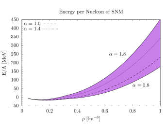
Figure 2: Density dependence of the energy per nucleon of SNM computed varying the strength of the repulsive NNN potential $\alpha_{R}$, defined by Eq. (1), in the range $0.8\leq\alpha\leq 1.8$.

I.2 Speed of sound

The results of Fig. 2 clearly show that the strength of the NNN repulsive potential strongly affects the matter pressure

$$P=\varrho^{2}\frac{\partial(E/A)}{\partial\varrho}\ ,$$ (11)

which in turn determines the speed of sound, $v_{s}$, defined through

$$v^{2}_{s}=\frac{1}{\varrho}\frac{\partial P}{\partial(E/A)}\ .$$ (12)

In Fig. 3, the pressure of SNM corresponding to different values of $\alpha$ is displayed as a function of density. For comparison, the shaded area shows the region consistent with the experimental data discussed in Ref. P. Danielewicz, R. Lacey, and W. G. Lynch (2002), providing a constraint on $P(\varrho)$ at $\varrho\geq 2\varrho_{0}$.

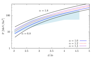
Figure 3: Density dependence of the pressure of SNM, obtained using the parametrisation of $V^{R}_{ijk}$ of Eq. (3) with $0.8\leq\alpha\leq 1.8$. The shaded region represents the results of the analysis of Ref.  P. Danielewicz, R. Lacey, and W. G. Lynch (2002).

Being non relativistic in nature, the approach based on the Hamiltonian of Eq.(1) unavoidably leads to a violation of causality—signalled by a speed of sound exceeding unity—in the limit of large density. The results of Fig. 4, obtained using the parametrisation of $V^{R}_{ijk}$ of Eq. (3) with $0.8\leq\alpha\leq 1.8$, show that in $\beta$-stable matter with $\alpha=1$ the region of $c^{2}_{s}>1$ corresponds to energy density $\epsilon\gtrsim 6.5\epsilon_{0}$, while for larger values of $\alpha$ the violation of causality is pushed to $\epsilon$ as low as $\sim 4\epsilon_{0}$. Here, $\epsilon_{0}=2.67\times 10^{14}\ {\rm g\ cm}^{-3}$ is the mass density of a system of nucleons at number density $\varrho_{0}$.

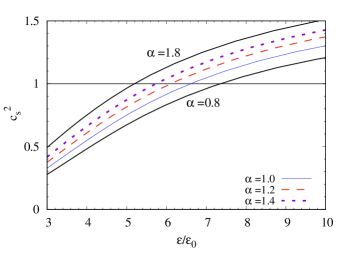
Figure 4: Energy density dependence of the squared speed of sound in $\beta$-stable matter, obtained using the parametrisation of $V^{R}_{ijk}$ of Eq. (3) with $0.8\leq\alpha\leq 1.8$.

The capability of the dynamical model employed in this work to support a NS of mass compatible with the observational constraints can be gauged comparing the results of Figs. 4 and 5. The dependence of the NS mass of—obtained from the solution of the Tolman-Oppenheimer-Volkoff (TOV) equations—on the central energy density, $\epsilon_{c}$, clearly shows that all EOSs corrresponding to $0.8\leq\alpha\leq 1.8$ predict a stable NS with mass exceeding two solar masses, and central densities well below the region corresponding to $c_{s}^{2}>1$.

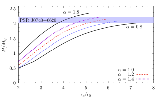
Figure 5: Energy density dependence of the NS mass, obtained from the solution of the TOV equations using the parametrisation of $V^{R}_{ijk}$ of Eq. (3) with $0.8\leq\alpha\leq 1.8$. All curves extend to the maximum value of density for which the speed of sound in matter satisfies the causality constraint $v_{s}<1$.

II Frequencies of non-Radial Oscillation Modes

In this work, we analyse the influence of the strength of the repulsive NNN forces on the gravitational radiation emitted by a NS following the excitation of the non-radial $f$ mode Thorne and Campolattaro (1967, 1968). For any assigned EOS of NS matter, the frequencies of QNMs can be obtained by studying the source-free, adiabatic perturbations of an equilibrium configuration. This involves solving the linearised Einstein equations, coupled with the equations of hydrodynamics, with suitably posed boundary conditions.

The unperturbed configuration is assumed to be a static spherically symmetric star, whose geometry is described by the line element

$$(ds^{2})^{(B)}=-e^{2\nu}dt^{2}+e^{2\lambda}dr^{2}+r^{2}(d\theta^{2}+\sin^{2}{\theta}d\phi^{2}),$$ (13)

where $\nu$ and $\lambda$ are functions of $r$, and $\lambda$ is related to the gravitational mass comprised within a sphere of radius $r$, $M(r)$, through

$$e^{-\lambda}=\left[1-2\frac{M(r)}{r}\right]^{1/2}\ .$$ (14)

Denoting by $\epsilon(r)$ and $p(r)$ the total energy density and pressure measured in the proper frame of the fluid, we can write the Tolman-Oppenheimer-Volkoff (TOV) equations in the form

$$\frac{dM}{dr} =4\pi r^{2}\epsilon\ ,$$ (15)

$$\frac{dp}{dr} =-\frac{(\epsilon+p)(M+4\pi r^{3}p)}{r(r-2M)}\ ,$$ (16)

$$\frac{d\nu}{dr} =-\frac{1}{(\epsilon+p)}\frac{dp}{dr}\ ,$$ (17)

with the boundary conditions

$$M(0) =0\ \ ,\ \ p(R)=0\ ,$$ (18)

$$\nu(R) =\frac{1}{2}\ln\bigg{(}1-\frac{2M(R)}{R}\bigg{)}\ .$$ (19)

Here, we write the perturbed line element in the form Detweiler and Lindblom (1985)

$$ds^{2}= -e^{2\nu}(1+r^{l}H_{0}Y^{l}_{m}e^{i\omega t})dt^{2}$$ (20)

$$-2i\omega r^{l+1}H_{1}Y^{l}_{m}e^{i\omega t}dtdr$$

$$+e^{2\lambda}(1-r^{l}H_{0}Y^{l}_{m}e^{i\omega t})dr^{2}$$

$$+r^{2}(1-r^{l}KY^{l}_{m}e^{i\omega t})(d\theta^{2}+\sin^{2}{\theta}d\phi^{2}),$$

where the functions $Y_{lm}(\theta,\phi)$ are spherical harmonics. The small amplitude motion of the perturbed configuration is described by the Lagrangian 3-vector fluid displacement $\xi^{j}$, which can be represented in terms of perturbation functions $W(r)$ and $V(r)$ as

$$\xi^{r} = r^{l-1}e^{-\lambda}W(r)Y^{l}_{m}e^{i\omega t},$$ (21)

$$\xi^{\theta} = -r^{l-2}V(r)\partial_{\theta}Y^{l}_{m}e^{i\omega t},$$ (22)

$$\xi^{\phi} = -\frac{r}{(r\ \sin\theta)^{2}}V(r)\partial_{\phi}Y^{l}_{m}e^{i\omega t}.$$ (23)

Our analysis will be restricted to the $l=2$ component. Introducing the variable $X$, defined as

$$X =\omega^{2}(\epsilon+p)e^{-\nu}V-r^{-1}p,_{r}e^{(\nu-\lambda)}W$$ (24)

$$+\frac{1}{2}(\epsilon+p)e^{\nu}H_{0}\ ,$$

where the notation $,_{r}$ indicates differentiation with respect to $r$, it is possible to write a fourth-order system of linear differential equations for the functions $H_{1}$, $Z$, $W$, and $X$ Lindblom and Detweiler (1983); Detweiler and Lindblom (1985)

$$K,_{r} =\frac{H_{0}}{r}+\frac{l(l+1)}{2r}H_{1}-\left[\frac{(l+1)}{r}-\nu,_{r}\right]K$$

$$-8\pi(\epsilon+p)\frac{e^{\lambda}}{r}W\ ,$$ (25)

$$H_{1},_{r} =-\frac{1}{r}\left[l+1+2M\frac{e^{2\lambda}}{r}+4\pi r^{2}e^{2\lambda}(p-\epsilon)\right]H_{1}$$

$$+\frac{e^{2\lambda}}{r}\left[H_{0}+K-16\pi(\epsilon+p)V\right]\ ,$$ (26)

$$W,_{r} =-\frac{(l+1)}{r}W+re^{\lambda}\left[\frac{1}{\gamma p}e^{-\nu}X\right.$$

$$-\left.\frac{l(l+1)}{r^{2}}V+\frac{1}{2}H_{0}+K\right]\ ,$$ (27)

$$X,_{r} =-\frac{l}{r}X+(\epsilon+p)e^{\nu}\left\{\frac{1}{2}\left(\frac{1}{r}-\nu,_{r}\right)H_{0}\right.$$

$$+\frac{1}{2}\left[r\omega^{2}e^{-2\nu}+\frac{1}{2}\frac{l(l+1)}{r}\right]H_{1}+\frac{1}{2}\left(3\nu,_{r}-\frac{1}{r}\right)K$$

$$-\frac{l(l+1)\nu,_{r}}{r^{2}}V-\frac{1}{r}\bigg{[}4\pi(\epsilon+p)e^{\lambda}$$

$$+\left.\omega^{2}e^{\lambda-2\nu}-r^{2}\left(\frac{e^{-\lambda}\nu,_{r}}{r^{2}}\right),_{r}\bigg{]}W\right\}\ .$$ (28)

In the above equations, $\gamma$ is the adiabatic index defined by

$$\gamma=\frac{(\epsilon+p)}{p}\frac{\Delta p}{\Delta\epsilon},$$ (29)

and $H_{0}$ can be taken out using

$$\left[3M+\frac{1}{2}(l+2)(l-1)r+4\pi r^{3}p\right]H_{0}=8\pi r^{3}e^{-\nu}X$$

$$\ \ \ \ \ \ \ -\left[\frac{1}{2}l(l+1)(M+4\pi r^{3}p)-\omega^{2}r^{3}e^{-2(\lambda+\nu)}\right]H_{1}$$

$$\ \ \ \ \ \ \ +\bigg{[}\frac{1}{2}(l+2)(l-1)r-\omega^{2}r^{3}e^{-2\nu}$$ (30)

$$\ \ \ \ \ \ \ -\frac{1}{r}e^{2\lambda}(M+4\pi r^{3}p)(3M-r+4\pi r^{3}p)\bigg{]}K.$$

The following boundary conditions need to be satisfied: (i) the perturbation functions must be finite everywhere, particularly at $r=$0 where the system becomes singular, and (ii) the perturbed pressure must vanish at the surface of the star, corresponding to $r=R$, at any time, implying $\Delta p(R)$=0. From the relation Sotani et al. (2011)

$$\Delta p=-r^{l}e^{-\nu}X\ ,$$ (31)

it follows immediately that $\Delta p(R)$=0 also implies $X(R)=$0. For a given set of $l$ and $\omega$, there is a unique solution which satisfies all of the boundary conditions.

To solve the equations numerically we expand the solutions at $r=$0 and $r=R$, according to a procedure suggested by Lindblom and Detweiler Lindblom and Detweiler (1983); Detweiler and Lindblom (1985) and refined by the authors of Ref. Lü and Suen (2011).

Outside the star all quantities associated with the fluid vanish, and the perturbation equations reduce to the Zerilli equation Zerilli (1970); Fackerell (1971); Chandrasekhar and Detweiler (1975)

$$\frac{d^{2}Z}{dr^{*2}}+[\omega^{2}-V(r^{*})]Z=0\ ,$$ (32)

where the effective potential $V(r^{*})$ is written as

$$V(r^{*}) = \frac{2(1-2M/r)}{r^{3}(nr+3M)^{2}}\Big{[}n^{2}(n+1)r^{3}+3n^{2}Mr^{2}$$ (33)

$$+9nM^{2}r+9M^{3}\Big{]}\ ,$$

with $n=(l-1)(l+2)/2$, and $r^{*}$ is the “tortoise” coordinate, which can be written in terms of $r$ as

$$r^{*}=r+2M\log\left(\frac{r}{2M}-1\right)\ .$$ (34)

In terms of $H_{0}(r)$ and $K(r)$, the Zerilli function $Z(r^{*})$ and its derivative are

$$Z(r^{*}) =\frac{k(r)K(r)-a(r)H_{0}(r)-b(r)K(r)}{k(r)g(r)-h(r)},$$ (35)

$$\frac{dZ(r^{*})}{dr^{*}} =\frac{h(r)K(r)-a(r)g(r)H_{0}(r)-b(r)g(r)K(r)}{h(r)-k(r)g(r)},$$ (36)

with Lü and Suen (2011)

$$a(r) =-\frac{(nr+3M)}{[\omega^{2}r^{2}-(n+1)M/r]}\ ,$$ (37)

$$b(r) =\frac{[nr(r-2M)-\omega^{2}r^{4}+M(r-3M)]}{(r-2M)[\omega^{2}r^{2}-(n+1)M/r]},$$ (38)

$$g(r) =\frac{[n(n+1)r^{2}+3nMr+6M^{2}]}{r^{2}(nr+3M)},$$ (39)

$$h(r) =\frac{[-nr^{2}+3nMr+3M^{2}]}{(r-2M)(nr+3M)},$$ (40)

$$k(r) =-\frac{r^{2}}{(r-2M)}\ .$$ (41)

The Zerilli equation has two linearly independent solutions $Z_{+}(r^{*})$ and $Z_{-}(r^{*})$. They correspond to incoming and outgoing GWs, respectively. The general solution for $Z(r^{*})$ is given by the linear combination

$$Z(r^{*})=A(\omega)Z_{-}(r^{*})+B(\omega)Z_{+}(r^{*}).$$ (42)

At large $r$, $Z_{+}$ and $Z_{-}$ can be conveniently expanded according to

$$Z_{-}(r^{*}) =e^{-i\omega r^{*}}\sum_{j=0}^{\infty}\beta_{j}r^{-j},$$ (43)

$$Z_{+}(r^{*}) =e^{i\omega r^{*}}\sum_{j=0}^{\infty}\overline{\beta}_{j}r^{-j},$$ (44)

where ${\overline{\beta}}_{j}$ denotes the complex conjugate of $\beta_{j}$. Keeping only terms up to $j=\mathrm{2}$ and substituting Eq. (43) into Eq. (32), we obtain Lü and Suen (2011)

$$\beta_{1} =-i(n+1)\omega^{-1}\beta_{0},$$ (45)

$$\beta_{2}=-\omega^{2} \left[\frac{1}{2}n(n+1)-\frac{3}{2}iM\omega\left(1+\frac{2}{n}\right)\right]\beta_{0}.$$ (46)

As we are interested in purely outgoing radiation, we must find the value of $\omega$ satisfying $B(\omega)=0$, which is the frequency of the desired QNM.

III Numerical Results

Changing the strength of the repulsive contribution to the NNN potential, $V^{R}_{ijk}$, obviously affects the stiffness of the EOS of $\beta$-stable matter, see Sect. I.2. This effect is clearly illustrated in Fig. 6, showing that higher values of $\alpha$ increase both the stellar maximum mass and the radius. At both $M=\mathrm{1.4}\ M_{\odot}$ and $M=\mathrm{2}\ M_{\odot}$, increasing the value of $\alpha$ from 1 to 1.6 leads to $\sim$ 10 % increase of the star radius.

The pattern emerging from Fig. 6, indicating that the mass-radius relations are ordered according the value of $\alpha$—which in turn determines the stiffness—is largely reflected by the results displayed in the top panel of Fig. 7, showing the pulsation frequencies of the $f$ mode, $f=\mathrm{Re}\{\omega\}/2\pi$, as a function of the star mass. The different curves correspond to different values of $\alpha$ in the range $0.8\leq\alpha\leq 1.8$. Note that the multimessenger analysis of Ref. Maselli et al. (2021)—in which the stronger constraint turns out to be the bound on the maximum mass provided by PSR J0740+6620—yields a probability distribution for $\alpha$ that, while being compatible with the value $\alpha=1$, corresponding to the APR EOS, shows large support for $\alpha>1$, corresponding to stronger NNN repulsion and stiffer EOSs. The role of stiffness in the determination of the tidal polarizability $\Lambda$ has been also discussed in Ref. Sabatucci and Benhar (2020), whose authors compared the results of calculations performed using EOSs obtained from different models of nuclear dynamics.

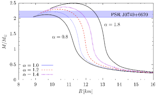
Figure 6: Mass radius relations of the stable NS configurations obtained using the EOSs corresponding to the nuclear Hamiltonian discussed in Sect. I. The curves are labelled according to the value of the parameter $\alpha$, defined in Sect. I.1 .

It is apparent that increasing $\alpha$ results in sizeably lower values of the frequency. A comparison between the cases $\alpha=0.8$ and $\alpha=1.8$ at $M=\mathrm{1.4\ M_{\odot}}$ shows a decrease of $\sim 20$%, from 2.1 kHz to 1.68 kHz. The same percentage decrease, from 2.42 kHz to 1.92 kHz is found at $M=\mathrm{2\ M_{\odot}}$. The mass-independence of the effect of using EOSs featuring different stiffness is a remarkable property, that was already pointed out, in a somewhat different context, by the authors of Ref. O. Benhar, E. Berti, and V. Ferrari (1999).

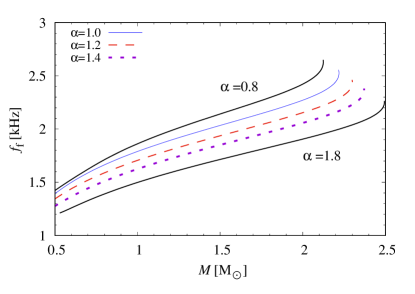
Figure 7: Top panel: frequency of the $f$ mode of stable NSs configurations obtained using the nuclear Hamiltonian discussed in Sect. I.1. The curves are labelled by the value of the parameter $\alpha$, determining the strength of repulsive NNN interactions. Bottom panel: same as the top panel, but for the damping time $\tau=\mathrm{1/Im}\{\omega\}$

On the other hand, the bottom panel of Fig. 7 shows that the damping times $\tau=\mathrm{1/Im}\{\omega\}$ corresponding to different values of $\alpha$ are much closer to one another. Moreover, they are not ordered according to the stiffness of the underlying EOSs over the whole range of mass.

IV Summary and Conclusions

We have studied the dependence of the frequencies and damping time of the NSs’ $f$ mode on the strength of repulsive NNN forces. Improving the available NNN potential models is of outmost importance for astrophysical applications, because NNN interactions, while playing a critical role in the determination of the nuclear matter EOS at high densities, is not strongly constrained by nuclear data

In our dynamical model, the repulsive contribution to the UIX NNN potential of the APR Hamiltonian is modified through the action of the parameter $\alpha$. The APR model, providing the baseline of the analysis, corresponds to $\alpha=1$, and larger values of $\alpha$ lead to stiffer EOSs. Based on the results of Ref. Maselli et al. (2021), we have considered the range $0.8\leq\alpha\leq 1.8$.

We find that the frequency of the $f$ mode is significantly affected by the strength of the NNN potential over the whole range of stellar masses, while the damping time turns out to be largely independent of $\alpha$. These results suggest that, with a galactic supernova event, we may be able to exploit the detection of gravitational radiation associated with the excitation of the QNM to constrain the value $\alpha$. However, GW observations coming from mergers may offer a more promising scenario.

The most important way of analysing the influence of QNMs in a merger waveform would be taking into account the effects of dynamical tides Andersson (2021); G. Pratten, P. Schmidt, and T. Hinderer (2020); Steinhoff et al. (2021); Schmidt and Hinderer (2019); Andersson and Pnigouras (2021). As the binary evolves towards merger, variations in the tidal fields reach a resonance with the star’s internal oscillation modes, creating new particular features in the GW waveform that can be detected and provide information on the QNMs; amongst these modes, the $f$ mode is the most important one G. Pratten, P. Schmidt, and T. Hinderer (2020). Most notably, Ref. G. Pratten, P. Schmidt, and T. Hinderer (2020) has shown promising results that we will be able to measure the $f$-frequency from GW inspirals to within of Hz in the future GW detector networks. At this stage, we would be able to directly infer how strong $V_{ijk}^{R}$ is, as the differences we get are of hundreds of hertz. As also noted in their work, GW170817 rules out EOSs that produce very low $f$ frequencies, corresponding to very stiff EOSs and higher values of $\alpha$.

Exploring the post-merger signal is another way of gathering information on the $f$ mode of static stars. This scenario consists of a rapidly evolving background spacetime, but even so the peak frequency of GW emission is related to the $f$ mode Stergioulas et al. (2011); Vretinaris et al. (2020) and moreover, we can establish relations between this frequency and the one of static stars Chakravarti and Andersson (2020); Lioutas et al. (2021); Bernuzzi et al. (2015). In the next generation of GW detectors we would be able to detect the post-merger signal, which in turn would give us the possibility of constraining the $f$ frequency of the inspiral phase, allowing to have another valuable information about the internal composition of NSs.