[subsection]section *[subsection]section

1 Introduction

In 2009 D. Gaiotto, G. Moore and A. Neitzke published a theory which they argued would lead to a very concrete way of constructing hyperkähler metrics on a large class of different manifolds using twistor theory on integrable systems. The general theory was first presented in [GMN10] and in [GMN13a] an explicit adaptation for the moduli space $\mathcal{M}$ of weakly parabolic Higgs bundles on a compact Riemann surface $\mathcal{C}$ was developed which also introduced the notion of spectral networks that were further developed in [GMN13]. While their general theory remained conjectural, a lot of progress has been made since then, proving some of their conjectures in certain special cases. In 2017 C. Garza was able to show in [Gar17] how the construction works for the so called Pentagon case, an integrable system with torus fibers that exhibit some nodal structure on a certain locus, very similar to the known behavior of the Higgs bundle moduli space. Notably he was able to show how the Ooguri-Vafa metric is a suitable model for the singular fibers. The most recent step in this direction was taken by I. Tulli, who showed in [Tul19] how the construction works on a specific moduli space of framed wild harmonic bundles on $\mathbb{CP}^{1}$. Thus the progress in the general theory has mostly been made for very specific examples while the conjectures were intended for a much broader context.

One of the most prominent conjectures of Gaiotto, Moore and Neitzke (GMN) concerns the comparison of the natural $L^{2}$-metric $g_{L^{2}}$ which is defined on all of $\mathcal{M}$ and the semiflat metric $g_{\text{sf}}$ for large Higgs fields, which is defined on the regular locus $\mathcal{M}^{\prime}\subset\mathcal{M}$ where determinants of the Higgs field have only simple zeroes. GMN argued for the exponential decay of the difference of these to metrics on $\mathcal{M}^{\prime}$ for large Higgs fields, i. e. when considering generic Higgs bundles $(\mathcal{E},R\Phi)$ for large $R$ the difference of the two metrics should be $g_{L^{2}}-g_{\text{sf}}=O\left(e^{-\gamma R}\right)$. Additionally they conjectured that $\gamma$ is given by the length of the shortest saddle connection in the metric on $\mathcal{C}$ induced by Det$\Phi$. This problem was later also tackled by R. Mazzeo, J. Swoboda, H. Weiß and F. Witt using different methods for the case of regular $\text{SU}(2)$-Higgs bundles in [Maz+12], [Maz+16] and [Maz+19]. They were able to prove a polynomial decay by introducing the notion of limiting configurations. For large Higgs fields these almost solve Hitchin’s equations, leaving only an exponentially small remainder term which allows for good approximations of the natural metric. The decay rate was later on improved to be an actual exponential decay by D. Dumas and A. Neitzke for a special case in [DN19] and in generality by L. Fredrickson in [Fre20], who also expanded the theory for the $\text{SU}(N)$ case in [Fre18].

Although it seemed reasonable to suspect that the two theories (twistorial construction on the integrable system and limiting configurations) could complement each other they weren’t put together on a general class of Higgs bundle moduli spaces until now, as the twistorial construction needs to consider Higgs bundles with singularities while the limiting configurations until recently were only developed for regular Higgs bundles. But this has changed now as L. Fredrickson, R. Mazzeo, J. Swoboda and H. Weiß (FMSW) were able to develop their theory for the weakly and strongly parabolic Higgs bundles in [Fre+20]. This finally allows to merge both theories and show that they fit together quite nicely as they give very concrete expressions and good approximations for a lot of important objects on $\mathcal{M}$, namely a set of Darboux coordinates, a holomorphic symplectic form and a hyperkähler metric. Thus we will argue in this article that the conjectural picture of GMN works for moduli spaces of weakly parabolic Higgs bundles of rank $2$ on Riemann surfaces of arbitrary genus with an arbitrary number of parabolic points. In particular a hyperkähler metric can be constructed in a twistorial way whose difference to the semiflat metric decays exponentially with the conjectured optimal decay rate.

Let us briefly summarize the key steps in the construction which will serve as a guide for our endeavor. One starts with the moduli space of weakly parabolic Higgs bundles regarded as a space of Higgs pairs $(\Phi,A)$ consisting of a Higgs field $\Phi$ and a connection $A$ on some fixed rank $2$ vector bundle $V$ over a Riemann surface $\mathcal{C}$. The basic theory of this moduli space will be explained in section 2 where we mostly follow the set up of [Fre+20], as their results are fundamental for our work here.

To each Higgs pair one then associates a decorated triangulation of $\mathcal{C}$. This entails a triangulation of $\mathcal{C}$ that is given by certain curves that are geodesics when considered in the metric on $\mathcal{C}$ induced by Det$\Phi$. On the other hand the decoration consists of a choice of a $1$-dimensional subspace of $V$ at each vertex of the triangulation. In our setting this subspace if given by a solution $s$ to the flatness equation $\nabla(\zeta)s=0$ where $\nabla(\zeta)=\tfrac{R}{\zeta}\Phi+A+R\zeta\Phi^{\ast}$ (for $R$ positive and $\zeta$ a complex valued parameter) is a connection on $V$ that is flat for bundles of parabolic degree $0$. We will constrain ourselves to this case and describe the restriction later on in more detail. As V. Fock and A. Goncharov proved in [FG06], one can construct a coordinate system for the moduli space of flat connections out of these decorated triangulations. Following [GMN13a] section 3 will be concerned with constructing the triangulation and explaining how the coordinates of Fock and Goncharov relate to coordinates of the Higgs bundle moduli space.

The main difficulty in this construction comes from solving the flatness equation. Locally this is a non-autonomous linear ODE whose components are only partially known. For the construction to work, one has to be able to chose certain solutions in a unique way (up to scalar multiplication) such that they have the right asymptotics for $\zeta\to 0$ and $\zeta\to\infty$. The existence of such sections, called small flat sections, was conjectured in [GMN13a], but has not been rigorously proven until now. In section 4 we will use the results of [Fre+20] to obtain a local description of Higgs pairs as the sum of a diagonal leading term and a remainder that is exponentially suppressed, the general idea being that if the connection matrix of $\nabla(\zeta)$ has this composite form, then the solutions of $\nabla(\zeta)=0$ should also be determined by an explicitly known leading term and some remainder that is exponentially suppressed.

In [GMN13a] GMN already used an argument along these lines, where they used the WKB approximation to conjecture the right behaviour of the solutions. Here we will not use this approach but instead develop a rigorous theory of ”initial value problems at infinity” in section 5 which expands the existing theory of Volterra integral equations. Explicitly we show the unique existence, as well as the continuous and differentiable dependence on parameters of solutions to Volterra equations of the second kind on unbounded intervals for a general class of integral kernels. This theory hadn’t been developed before and might also be useful in different contexts.

With the tools of this theory at hand we then proceed to section 6, where we study the solutions to the flatness equation and obtain our first main result.

Theorem 1.1

At each weakly parabolic point of a Higgs bundle in $\mathcal{M}^{\prime}$ there exists a solution of the flatness equation that is unique up to scalar multiplication and s. t. the Fock-Goncharov coordinates constructed out of these decorations are of the form

$$\mathcal{X}=(1+r)\exp\left(\frac{R}{\zeta}\pi Z+i\theta+R\zeta\pi\overline{Z}\right),$$

where $r$ is exponentially suppressed in $R$ and $Z$ and $\theta$ are coordinates of the Hitchin fibration.

We note here that the calculations necessary for this theorem show that the combination of our theory of initial value problems at infinity and the theory of geodesics for quadratic differentials is a very good tool for the general problem of parallel transport.

The $\mathcal{X}$-coordinates thus constructed are defined on $\mathcal{M}^{\prime}$ for generic values of $\zeta\in\mathbb{C}^{\ast}$ and can be associated to elements of the lattice $\Gamma_{q}\subset H_{1}(\Sigma^{\prime}_{q};\mathbb{Z})$ on the spectral cover $\Sigma_{q}$ of $\mathcal{C}$ corresponding to the derminant $q$ of the Higgs field. For specific rays in $\mathbb{C}^{\ast}$ the underlying triangulation on $\mathcal{C}$ changes, which leads to jumps of the coordinates. For a certain generic subset $\widetilde{\mathcal{M}}^{\prime}_{R,c}\subset\mathcal{M}^{\prime}$ the jumps are completely understood and can be used to formulate a Riemann-Hilbert problem which is then solved by the $\mathcal{X}$-coordinates. We show how this is done in section 7. Our main Theorem in that section then concerns a certain integral equation which was proposed by GMN for the general construction of Hyperkähler metrics on integrable system, where the jumps are determined by certain so called (generalized) Donaldson-Thomas invariants $\Omega$.

Theorem 1.2

The $\mathcal{X}$-coordinates are solutions to the integral equation

$$\mathcal{X}_{\gamma}(\zeta)=A_{\gamma}\mathcal{X}_{\gamma}^{\text{sf}}(\zeta)\text{exp}\left[-\frac{1}{4\pi i}\sum_{\beta\in\Gamma_{q}}\Omega(\beta;q)\left\langle\gamma,\beta\right\rangle\int_{l_{\beta}(q)}\frac{d\zeta^{\prime}}{\zeta^{\prime}}\frac{\zeta^{\prime}+\zeta}{\zeta^{\prime}-\zeta}\log\left(1-\mathcal{X}_{\beta}(x,\zeta^{\prime})\right)\right],$$

for some constant $A_{\gamma}\in\mathbb{C}$ with $\left\|A_{\gamma}\right\|=1$ which is exponentially close $1$ for large $R$.

In our setting the consideration of this integral equation has the advantage that we obtain additional analytic details regarding certain asymptotics of the $\mathcal{X}$-coordinates.

Coming back to the general construction, the idea proposed by GMN is that the $\mathcal{X}$ coordinates fit into the picture of [GMN10], i. e. one can use them to construct a holomorphic symplectic form from which one can construct the hyperkähler metric on the moduli space by use of the twistor theorem of N. J. Hitchin, A. Karlhede, U. Lindström and M. Ro$\check{\text{c}}$ek. We will explain this general construction of GMN in the final section 8. Here we just note that it is the use of the twistor theorem for which the $\zeta$-asymptotics of the $\mathcal{X}$-coordinates and their derivatives have to be known. Only then one may obtain such a twistorial hyperkähler metric. As it turns out our theory is strong enough to also obtain these right asymptotics and thus obtain the final result.

Theorem 1.3

There is a hyperkähler metric on $\widetilde{\mathcal{M}}^{\prime}_{R,c}$ constructed by the twistorial method whose difference to the semiflat metric decays exponentially in $R$. Furthermore the decay rate is given by the minimal period $2\pi R|Z_{\mu}|$, where $Z_{\mu}$ is the minimal period integral $\oint_{\mu}q^{1/2}$ for $\mu\in\Gamma_{q}$ with $\Omega(\mu)\neq 0$.

We note here that we do not yet know that our twistorial hyperkähler metric is the natural $L^{2}$ metric on the moduli space. It is natural to conjecture this at this point and we will sketch an outline of a possible proof at the end of the last section, which was communicated to us by Andrew Neitzke.

Acknowledgments: I thank my advisor, Harmut Weiß, for many helpful discussions and advices. I also want to thank Andrew Neitzke for clarifying important aspects of the general theory. I received reimbursement of travel expenses from the DFG SPP 2026.

2 Parabolic Higgs bundles

In this section we start by developing the basic constructions for the moduli space we are interested in. The presentation here mostly follows [Fre+20]. For the general construction and further details see also [Nak96] and [BY96]. We will start by giving an overview of parabolic Higgs bundles in subsection 2, which can roughly be described as Higgs bundles that may have singularities at certain fixed points. There are some different notions that will have to be separated there concerning the structure of the poles. One idea is to allow simple poles and residues of the Higgs field which are nilpotent. Those were introduced in [Kon93] and are called strongly parabolic with regular singularities. As it turns out our construction does at this moment not seem to work on the corresponding moduli space for these bundles. Nevertheless a thorough investigation of the possibilities of adapting the method presented here to that case would be highly interesting. Instead we will focus on weakly parabolic bundles which also have simple poles but allow for diagonalizable residues of the Higgs field. Finally there also is a moduli space for bundles with singularities of order $>1$. These are called wild or irregular, were presented in [BB04] and may also be strongly or weakly parabolic. For us they are of importance as an application of the theory presented here to a special case of wild bundles on the sphere was carried out in [Tul19], which shows that the theory can actually be adapted to different settings.

2.1 The moduli space of parabolic Higgs bundles.

Let $\mathcal{C}$ be a compact Riemann surface of genus $g$ with a metric $g_{C}$ and Kähler form $\omega_{C}$ and $E$ a $\mathcal{C}^{\infty}$-vector bundle over $\mathcal{C}$ of rank $r$ and degree $d$. This is the data that stays fixed throughout all of the following constructions. We also fix a holomorphic structure $\overline{\partial}_{\text{Det}E}$ on the complex line bundle $\text{Det}E=\Lambda^{r}E$ with associated Hermitian-Einstein metric $h_{\text{Det}E}$. This metric induces the Chern connection $A$ on this holomorphic Hermitian line bundle and is characterized by the curvature

$$F_{A}=-\sqrt{-1}\text{deg}E\frac{2\pi\omega_{\mathcal{C}}}{\text{vol}_{g_{\mathcal{C}}}(\mathcal{C})}\text{Id}_{\text{Det}E}$$

We can then equip $E$ with a holomorphic structure $\overline{\partial}_{E}$ demanding that $\overline{\partial}_{E}$ induces $\overline{\partial}_{\text{Det}E}$ on $\text{Det}E$ and denote by $\mathcal{E}\mathrel{\mathop{\mathchar 58\relax}}=(E,\overline{\partial}_{E})$ the emerging holomorphic vector bundle.

We now introduce the parabolic data which starts with a divisor $D=p_{1}+\ldots+p_{n}$ on $\mathcal{C}$, i. e. we fix $n$ distinct points on the surface. To these points we associate data that fixes the behavior of certain objects near them.

Definition 2.1

A parabolic structure on $E$ consists of a choice of weighted flags $\mathcal{F}(p)=F_{\bullet}(p)$, i. e.

$$\begin{split}E_{p}&=F_{1}(p)\supset\ldots\supset F_{s_{p}}(p)\supset 0\\ 0&\leq\alpha_{1}(p)<\ldots<\alpha_{s_{p}}(p)<1\end{split}$$

for each $p\in D$ with $\sum_{i=1}^{n}\alpha_{i}=1$. A vector bundle with parabolic structure is called a parabolic bundle.

Now let $K_{\mathcal{C}}$ be the canonical line bundle. We are interested Higgs fields that have simple poles at the marked points, which are defined as follows:

Definition 2.2

A parabolic Higgs field is a holomorphic bundle map $\Phi\mathrel{\mathop{\mathchar 58\relax}}\mathcal{E}\rightarrow\mathcal{E}\otimes K_{\mathcal{C}}(D)$ w. r. t. the induced holomorphic structure of $\overline{\partial}_{E}$. The Higgs field is said to preserve the parabolic structure if, for all $i$ and $p$ the residue preserves the flags, i. e.:

$$\text{res}_{p}\Phi(F_{i}(p))\subseteq F_{i}(p).$$

A parabolic Higgs bundle is a holomorphic vector bundle $\mathcal{E}$ together with a parabolic structure and a parabolic Higgs field $\Phi$ preserving the parabolic structure.

Note that the twist by $D$ in the definition amounts to $\Phi$ having simple poles, so we will also call the Higgs field and associated objects meromorphic. At this point there are two possibilities for the residue of $\Phi$. It may be nilpotent in which case the Higgs field is called strongly parabolic or it may be diagonalizable in which case it is called weakly parabolic. In the case of weakly parabolic bundles the residue data, i. e. the eigenvalues of the residue at each parabolic point shall also be fixed.

In the following we will only consider weakly parabolic bundles of rank $2$. Furthermore we restrict ourselves to the $SL(2,\mathbb{C})$ case. For the definition we state all the fixed data.

Definition 2.3

Let $E$ be a complex rank $2$ vector bundle over a compact Riemann surface of degree $d$, together with a divisor $D=p_{1}+\ldots+p_{n}$ and holomorphic structure $\overline{\partial}_{\text{Det}E}$ on $\text{Det}E$. Furthermore for each $p\in D$ let a weight vector $\vec{\alpha}(p)=(\alpha_{1}(p),\alpha_{2}(p))\in[0,1)^{2}$ with $\alpha_{1}(p)+\alpha_{2}(p)=1$ be given, as well as $\sigma_{p}\in\mathbb{C}^{\times}$.

A weakly parabolic $SL(2,\mathbb{C})$-Higgs bundle over $(\mathcal{C},D)$ is a triple $(\overline{\partial}_{E},\left\{\mathcal{F}(p)\right\}_{p\in D},\Phi)$, where $\overline{\partial}_{E}$ is a holomorphic structure on $E$ inducing $\overline{\partial}_{\text{Det}E}$, $\mathcal{F}(p)$ is a complete flag for each $p\in D$ and $\Phi\mathrel{\mathop{\mathchar 58\relax}}\mathcal{E}\rightarrow\mathcal{E}\otimes K_{\mathcal{C}}(D)$ is a Higgs field which is traceless with residue eigenvalues $\sigma_{p}$ and $-\sigma_{p}$ at each $p\in D$.

It is useful to write $\mathcal{E}$ for the holomorphic bundle $(E,\overline{\partial}_{E})$ together with the flag, s. t. a parabolic Higgs bundle may be expressed as a pair $(\mathcal{E},\Phi)$ just as in the regular case.

To obtain a well behaving moduli space a notion of stability is necessary. For this one defines the (weight depended) parabolic degree of $\mathcal{E}$ as

$$\text{pdeg}_{\vec{\alpha}}(\mathcal{E})=\text{deg}(\mathcal{E})+\sum_{p\in D}(\alpha_{1}(p)+\alpha_{2}(p)).$$

A parabolic structure on $\mathcal{E}$ induces a parabolic structure on its holomorphic subbundles and so one defines $(\mathcal{E},\Phi)$ to be $\vec{\alpha}$-stable iff

$$\mu(\mathcal{E})\mathrel{\mathop{\mathchar 58\relax}}=\frac{\text{pdeg}_{\vec{\alpha}}(\mathcal{E})}{\text{rank}(\mathcal{E})}>\text{pdeg}_{\vec{\alpha}}\mathcal{L}.$$

for every holomorphic line subbundle $\mathcal{L}$ preserved by $\Phi$. Here $\mu(\mathcal{E})$ is the parabolic slope of $\mathcal{E}$. The notion of semistability follows if instead of $>$ one allows $\geq$ and the weights are called generic if any $\vec{\alpha}$-semistable bundle is $\vec{\alpha}$-stable.

For the definition of the moduli space we start by fixing the residues $\sigma=\left\{\sigma(p)\right\}_{p\in D}$ and the flags $\mathcal{F}(p)$ for each $p\in D$. We denote by SL$(E)$ the bundle of automorphisms of $E$ that induce the identity on Det$(E)$ and by $\mathfrak{sl}=\text{End}_{0}E$ the bundle of tracefree endomorphisms. Now denote by $\mathcal{A}_{0}$ the affine space of all holomorphic structures on $E$ that induce the fixed holomorphic structure $\overline{\partial}_{\text{Det}E}$ on Det$E$ and by $\mathcal{P}_{0,\sigma}\subset\Omega^{1,0}(\mathcal{C},\text{End}_{0}E)$ the set of sections of $\text{End}_{0}E\otimes K_{C}(D)$ (i. e. tracefree endomorphisms with simple poles), which are compatible with the flag and with residues $\sigma(p)$ and $-\sigma(p)$ at each $p\in D$.

We then start with the space

$$\mathcal{H}\mathrel{\mathop{\mathchar 58\relax}}=\left\{(\overline{\partial}_{E},\Phi)\in\mathcal{A}_{0}\times\mathcal{P}_{0,\sigma}\mathrel{\mathop{\mathchar 58\relax}}\Phi\text{ is meromorphic w. r. t. to }\overline{\partial}_{E}\right\}.$$

Now we fix a generic weight vector $\vec{\alpha}(p)$ at each $p\in D$ and denote by $\mathcal{H}_{\vec{\alpha}}$ the subspace of pairs $(\overline{\partial}_{E},\Phi)\in\mathcal{H}$ which are $\vec{\alpha}$-stable. For the gauge group let ParEnd$(E)$ be the bundle of automorphisms of $E$ that preserve the flag at each $p\in D$. Our gauge group will then be

$$\mathcal{G}_{\mathbb{C}}\mathrel{\mathop{\mathchar 58\relax}}=\Gamma(\text{SL}(E)\cap\text{ParEnd}(E)).$$

Finally we obtain the moduli space of SL$(2,\mathbb{C})$-Higgs bundles $\mathcal{M}_{\text{Higgs}}\mathrel{\mathop{\mathchar 58\relax}}=\mathcal{H}_{\vec{\alpha}}/\mathcal{G}_{\mathbb{C}}$, which is a Hyperkähler manifold of dimension

$$\text{dim}_{\mathbb{C}}\mathcal{M}_{\text{Higgs}}=6(g-1)+2n$$

for $g$ the genus of $\mathcal{C}$ (cf. [BY96]). For further details see also [Yok93] and [Kon93].

2.2 Nonabelian Hodge correspondence

Although we usually talk about the Higgs bundle moduli space, the objects we are actually working with are most of the time not the Higgs bundles $(\mathcal{E},\Phi)$ but their associated Higgs pairs $(\Phi,D(\overline{\partial}_{E}))$, which we’ll introduce now.

Let $(\mathcal{E},\Phi)$ be a parabolic Higgs bundle. By adding a Hermitian metric $h$ on $E$ the holomorphic structure $\overline{\partial}_{E}$ canonically induces a connection $D(\overline{\partial}_{E},h)$ on $E$, the so called Chern connection. After choosing a base connection $D(\overline{\partial}_{E},h)$ can be identified with an endomorphism valued $1$-form $A$ and may also be written as $d_{A}$. Explicitly if $\overline{\partial}_{E}$ is locally $\overline{\partial}+A_{\overline{z}}d\overline{z}$ in an $h$-unitary frame then $d_{A}$ is simply given by $D(\overline{\partial}_{E},h)=d_{A}=d+A=d+A_{\overline{z}}d\overline{z}-(A_{\overline{z}})^{\ast_{h}}dz$ where $d$ is the standard differential. Depending on the situation the connection is referred to as $D(\overline{\partial}_{E},h)$, $d_{A}$ or simply $A$. We can thus search for a hermitian metric $h$, such that the pair $(\Phi,D(\overline{\partial}_{E},h))$ satisfies Hitchin’s equation

$$F^{\bot}_{D(\overline{\partial}_{E},h)}+\left[\Phi,\Phi^{\ast_{h}}\right]=0,$$ (1)

where

$$F^{\bot}_{D(\overline{\partial}_{E},h)}-F_{D(\overline{\partial}_{E},h)}=\sqrt{-1}\mu(E)\frac{2\pi\varpi_{\mathcal{C}}}{\text{vol}_{g_{\mathcal{C}}}(\mathcal{C})}\text{Id}_{\text{Det}E}.$$

Note that the right hand side matches the curvature of the fixed Chern connection on $\text{Det}E$. In this way $F^{\bot}_{D(\overline{\partial}_{E},h)}$ is the trace-free part of the curvature of $D(\overline{\partial}_{E},h)$.

As stated in [Fre+20] in the parabolic setting one expects the Hermitian metric to match the parabolic structure in a suitable sense. For this one has to consider filtrations of the sections of $\mathcal{E}\otimes\mathcal{O}_{\mathcal{C}}(\ast D)$, for $\mathcal{O}_{\mathcal{C}}(\ast D)$ the sheaf of algebras of rational functions with poles at $D$. A parabolic structure determines such a filtration, as does a Hermitian metric, and if these two filtrations coincide the Hermitian metric is said to be adapted to the parabolic structure. This can be expressed locally by demanding that near each $p\in D$ for a holomorphic basis of sections $e_{1},e_{2}$ with $e_{i}\in F_{i}(p)$ one has $h(s,s)\sim|z|^{2\alpha_{i}(p)}$. For further details on this see [Moc06].

With these constraints one can now uniquely solve Hitchin’s equation (1) in the class of Hermitian metrics $h$, adapted to the parabolic structure on $\mathcal{E}$ (cf. [Sim90]). Then one obtains one part of the nonabelian Hodge correspondence

$$\mathcal{M}_{\text{Higgs}}\to\mathcal{M},\enspace(\mathcal{E},\Phi)\mapsto(\mathcal{E},\Phi,h).$$

Here $\mathcal{M}$ is the space of solutions to Hitchin’s equations modulo gauge equivalence, where we consider the gauge group

$$\mathcal{G}=\Gamma(\text{SU}(E)\cap\text{ParEnd(E))}.$$

of $h_{0}$-unitary transformations. We note the action of the gauge group as

$$g\cdot\overline{\partial}_{E}=g\circ\overline{\partial}_{E}\circ g^{-1},\enspace g\cdot\Phi=g\Phi g^{-1}\enspace\text{and}\enspace(g\cdot h)(v,w)=h(gv,gw).$$

The action on $\overline{\partial}_{E}$ then leads to an induced action on the Chern connection $A$.

On the other side if we assume $\text{pdeg}_{\vec{\alpha}}(\mathcal{E})=0$ for simplicity then for every solution $h$ of Hitchin’s equation there is a flat $SL(2,\mathbb{C})$-connection $A(\overline{\partial}_{E},h)+\Phi+\Phi^{\ast}$. For our construction of the metric we will use a correspondence quite similar to this, with the difference being a scaling in Hitchin’s equation and a twist by the complex parameter $\zeta$.

2.3 Spectral data and integrable systems

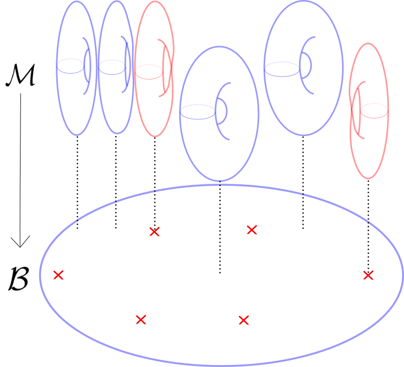
Figure 1: A subset of the Hitchin fibration in dimension $4$. The red crosses in the Hitchin base signify the elements of the discriminant locus over which the torus fibration becomes nodal.

Before we can start with the general idea of the construction of the Darboux coordinates on $\mathcal{M}_{R}$ we have to introduce a final feature, again following [Fre+20] where additional references are given. To every Higgs bundle $(\mathcal{E},\Phi)$ one can associate the characteristic polynomial $\text{char}_{\Phi}(\lambda)$ which does not depend on the parabolic structure. This gives rise to the Hitchin map

$$\text{Hit}\mathrel{\mathop{\mathchar 58\relax}}\mathcal{M}\to\mathcal{B},\quad(\mathcal{E},\Phi)\mapsto\text{char}_{\Phi}(\lambda).$$

Here $\mathcal{B}$ denotes the Hitchin base, identified with the affine space of coefficients of $\text{char}_{\Phi}(\lambda)$, so elements in $\mathcal{B}$ are collections of differential forms. In the case of SL$(2,\mathbb{C})$ bundles it holds $\text{tr}\Phi=0$ and thus the characteristic polynomial is just the determinant of $\Phi$.

For weakly parabolic bundles Det$\Phi$ is a meromorphic quadratic differential on $\mathcal{C}$ with a double pole of the the form $-\sigma^{2}\tfrac{dz^{2}}{z^{2}}$ near any weakly parabolic point $p$. One can associate a spectral curve $\Sigma\subset\text{Tot}\left(K_{\mathcal{C}}(D)\right)$ to each point in $\mathcal{B}$ which is a $2\mathrel{\mathop{\mathchar 58\relax}}1$ ramified cover of $\mathcal{C}$ in $K_{\mathcal{C}}(D)$, where each sheet represents a different eigenvalue of the Higgs field.

The subset $\mathcal{B}^{\prime}\subset\mathcal{B}$ of differentials in $\mathcal{B}$ that are generic, i. e. have only simple zeroes, are the ones for which $\Sigma$ is smooth. The following constructions will focus on the subset $\mathcal{M}^{\prime}\mathrel{\mathop{\mathchar 58\relax}}=\text{Hit}^{-1}(\mathcal{B}^{\prime})$ (and the corresponding $\mathcal{M}^{\prime}_{R}$) which is called the regular locus. Its complement is called the discriminant locus, cf. figure 1.

Lastly we want to mention the result going back to [Hit87] for the regular case that the Hitchin map equips $\mathcal{M}$ with the structure of an algebraically completely integrable system. Notably every fiber $\text{Hit}^{-1}(q)$ for each $q\in\mathcal{B}^{\prime}$ forms a torus which implies the notion of action angle-coordinates $Z,\theta$. Recovering these coordinates will be one of the main parts in the twistorial construction of the hyperkähler metrics.

3 Decorated triangulations and their coordinates

In this section we want to show how to build a (version of a) system of coordinates on the moduli space of flat connections on a Riemann surface $\mathcal{C}$ that was introduced by Fock and Goncharov in [FG06]. These coordinates are constructed via the data of triangulations on $\mathcal{C}$ together with a certain choice of decoration at each vertex. One crucial idea of GMN was, that the corresponding triangulations can be obtained from quadratic differentials which appear as the determinants of the Higgs fields and that the decorations correspond to solutions of a flatness equation for a certain connection build out of a solution of Hitchin’s equation. We stress that the entirety of this section is a summary of the construction of [GMN13a], and no new results are presented in the first three sections.

The theory presented in this section can mostly be considered independently of the theory of Higgs bundles and is interesting in its own right. So ignoring their possible origin as determinants we start in subsection 3.1 by introducing trajectories for arbitrary quadratic differentials and how a triangulation of $\mathcal{C}$ is build out of them. Most of this theory was developed by K. Strebel in [Str84]. We follow [GMN13a] in showing how to construct a triangulation with these trajectories and which phenomena may occur that are important for us. It should also be mentionend that these constructions and phenomena may be seen as an introduction to the theory of so called spectral networks that were introduced by GMN in [GMN13]. Since then they have become widely used and generalized especially in the physics literature. The theory shown here is just their simplest example which already entails quite a lot of the important structure of the general theory.

In subsection 3.2 we continue to present the work of [GMN13a], now turning to the construction of the decorations of the triangulation and how to build the Fock-Goncharov coordinate system out of them. Finally we will introduce the spectral curve in subsection 3.3 to obtain the full picture of the coordinate system. This is necessary to single out a certain subset of coordinates by use of the homology group of the spectral curve in order to obtain a set of coordinates that can later be identified as a sort of Darboux coordinate system.

Finally we have to consider what happens when we vary $\vartheta$. At certain values of $\vartheta$ the triangulation jumps which leads to corresponding jumps in the $\mathcal{X}$-coordinates. For the construction to work these jumps have to be of a certain kind and accordingly GMN carried out the analysis for the most important jumps in [GMN13a]. Still a certain phenomenon may appear if $\mathcal{C}$ has genus greater then $0$ which may pose a problem. We will introduce the important notions in section 3.4 and, using the work of T. Bridgeland and I. Smith [BS15], fill in some small gaps in the general theory.

3.1 $\vartheta$-trajectories and triangulations

We begin this section by recalling the construction of the $\vartheta$-triangulations which were introduced in [GMN13a] where they were called WKB triangulations. In the following $\mathcal{C}$ will always denote a compact Riemann surface. The foundational work for this section is [Str84] where all relevant facts are already given. We present the relevant results in this section and only mention those details which help getting an intuitive understanding of the phenomena that may occur. So nothing new is presented here and the representation mostly follows [GMN13a].

Definition 3.1

Given a meromorphic quadratic differential $q$ on (a subset of) $\mathcal{C}$ and $\vartheta\in\mathbb{R}/2\pi\mathbb{Z}$ a $\vartheta$-trajectory of $q$ is a curve $\gamma\mathrel{\mathop{\mathchar 58\relax}}I\to\mathcal{C}$ for some interval $I\subset\mathbb{R}$, s. t.

$$q\left(\gamma^{\prime},\gamma^{\prime}\right)\in e^{2i\vartheta}\mathbb{R}_{>0}.$$

Alternatively if $q$ has a well defined square root $q^{1/2}$ a $\vartheta$-trajectory of $q$ may be defined as any curve $\gamma\mathrel{\mathop{\mathchar 58\relax}}I\to\mathcal{C}$ for some interval $I\subset\mathbb{R}$, s. t.

$$q^{1/2}\left(\gamma^{\prime}\right)\in\mathbb{R}^{\times}e^{i\vartheta}.$$

Note that the second definition is more in line with calling the curve $\vartheta$-trajectory and is well defined, although the square root of $q$ is only defined up to sign. This amounts to the fact, that the $\vartheta$-trajectories are not oriented, i. e. if $\gamma(t)$ is a $\vartheta$-trajectory for $q$, so is $\gamma(-t)$ going in the opposite direction.

As we’ll explain below $\vartheta$-trajectories can be considered as straight lines with the inclination given by $\vartheta$ if considered in a suitable neighborhood. When talking about $\vartheta$-trajectories for varying $\vartheta$ it is also useful to have a notion that is independent of the specific angle and just reflects that each one is of such a constant angle.

Definition 3.2

Let $q$ be a meromorphic quadratic differential. A curve $\gamma\mathrel{\mathop{\mathchar 58\relax}}I\to\mathcal{C}$ shall be called a $ca$-trajectory of $q$ if there exists some $\vartheta\in\mathbb{R}/2\pi\mathbb{Z}$ s. t. $\gamma$ is a $\vartheta$-trajectory.

One important aspect of $ca$-trajectories is their behavior near zeroes and poles of the quadratic differential, which are called critical points in [FO08]. In the work of GMN the zeroes of $q$ are also called turning points and we’ll also use this notion at some places. In the following we are interested in a certain behavior that is exhibited by the $ca$-trajectories only if they have a specific kind of critical points, so we restrict our self to these differentials that are exactly the ones in the regular locus of the Hitchin base. Note however that a lot is also known about the $ca$-trajectories for differentials in the discriminant locus, so even though the following structures breaks down at these points, one may be able to get at least some information as to how the structure breaks down by further studies.

Definition 3.3

A generic differential is a meromorphic quadratic differential $q$ on $\mathcal{C}$, which has only poles of order $2$ and simple zeros.

When talking about certain standard behaviors (e. g. as growing or decaying) along a $ca$-trajectory it is useful to fix a standard for the parametrization, which we can always obtain.

Lemma 3.4

If $q$ is a generic differential there always exists a parametrization of its $\vartheta$-trajectories in which

$$q^{1/2}\left(\gamma^{\prime}\right)\in\pm e^{i\vartheta}.$$

This shall be called the standard parametrization of $\gamma$.

We now record the local structure of $ca$-trajectories near the different points we’ll encounter.

Lemma 3.5

Let $q$ be a generic differential, $\gamma$ a $\vartheta$-trajectory and $p$ one of the (second order) poles of $q$. Then $\gamma$ has one of the following forms in a local neighborhood around $p$:

• $\gamma$ is a logarithmic spiral running into (or away from) $p$.

• $\gamma$ is a circle with center $p$.

• $\gamma$ is a straight line running into $p$.

Proof.

Since $q$ is a meromorphic quadratic differential it is known from [Str84] that there exists a coordinate neighborhood $z$ with $z(p)=0$ and $q=(M/z^{2})dz^{2}$ for some complex number $M$. By shrinking our neighborhood we may thus assume, that $q^{1/2}$ is of the form $\tfrac{m}{z}dz$ for some constant $m$. Then we obtain the following general form of the WKB curve in the local coordinate:

$$z(t)=z_{0}e^{\pm\frac{e^{i\vartheta}}{m}t}.$$

Here $z_{0}$ is some complex constant. Depending on the specific values of $m$ and $\vartheta$ one of the three asserted possibilities occurs. ∎

For more details on this see [GMN13a] or, more generally, the original work of Strebel [Str84]. Here we note that in such a neighborhood for any given $\vartheta$ there are infinitely many $\vartheta$-trajectories running into the pole. This is contrasted by the $\vartheta$-trajectories running into the other exceptional points.

Lemma 3.6

Let $q$ be a generic differential and $p$ one of its (simple) zeros, i. e. a turning point. Then for any $\vartheta\in\mathbb{R}/2\pi\mathbb{Z}$ there are exactly three $\vartheta$-trajectories that run into the turning point.

Proof.

This can be shown by switching to a coordinate where $q=Mzdz^{2}$ and integrating the defining differential equation. ∎

Finally we are interested in the behavior away from any critical point.

Lemma 3.7

Let $q$ be a generic differential and $\vartheta\in\mathbb{R}/2\pi\mathbb{Z}$. Then in a local neighborhood around any regular point $p$ of $q$ the $\vartheta$-trajectories are a foliation by straight lines.

Proof.

In the coordinates $w(z)\mathrel{\mathop{\mathchar 58\relax}}=\int_{z_{0}}^{z}{q^{1/2}}$ the $\vartheta$-trajectories are a foliation by straight lines. ∎

Thus the behavior near every point of $\mathcal{C}$ is known and we obtain the following global picture.

Corollary 3.8

Let $q$ be a generic differential and $\vartheta\in\mathbb{R}/2\pi\mathbb{Z}$. Then the $\vartheta$-trajectories are the leaves of a (singular) foliation of $\mathcal{C}$

With this picture in mind we now classify the different kinds of $ca$-trajectories that may occur in the following list that exhaust all the possibilities.

Definition 3.9

Let $\gamma$ be a $\vartheta$-trajectory for generic differential $q$. It is called

• generic, iff it converges in both directions to a pole of $q$ (which may be the same for both directions).

• separating, iff it converges in one direction to a zero of $q$ and in the other direction to a pole of $q$.

• a saddle, iff it converges in both directions to a zero of $q$ (which may be the same for both directions).

• periodic, iff it is diffeomorphic to a circle and does not converge to any pole or zero of $q$.

• divergent, in all other cases. In this case $\gamma$ does in at least one direction not converge to a pole or zero of $q$.

As the name suggests almost all $ca$-trajectories in our setting will be generic and indeed most of our calculations will be along such trajectories. For this we’ll later on also need the following observation which we may already infer from the local behavior near their ”end points”.

Lemma 3.10

A generic $\vartheta$-trajectory in standard parametrization can be extended to all of $\mathbb{R}$.

Proof.

This follows from standard methods for ODEs. ∎

This infinite domain of the curve leads to the necessity of using integral equations with initial values at infinity later on as infinity corresponds to the poles of the quadratic differential.

Before we continue with the construction of the triangulation note the following remarks for some intuition concerning $ca$-trajectories:

First remember that $q$ was only defined up to sign which is why the $ca$-trajectories are not canonically oriented. The description of the behavior around poles as spiraling into the point may still be useful as a reminder what happens. Phenomenologically one might describe the singularities of $q$ as some (massive) object which ”captures” all curves, which come near enough. Thus finite curves have to be ”rare”. Indeed for one fixed $\vartheta$ their number is limited by the number of turning points and, even more, a curve coming from one turning point is more ”likely” to run into a singularity then another turning point. But the parentheses here are necessary when we talk about $ca$-trajectories of general quadratic differentials. For example one can show that on the four punctured sphere with a quadratic differential having only simple poles, for some angles only two finite $ca$-curves and one divergent curve exist which fill up the whole sphere. The angles for which such a behavior occurs even form a dense subset of $\mathbb{R}/2\pi\mathbb{Z}$. However, by working with generic quadratic differentials, the generic trajectories may safely be regarded as the ones which ”usually” occur, while finite curves don’t exist for most angles. This is why the following fact is crucial which was shown by GMN and which makes precise some of the vague formulations above.

Proposition 3.11

Let $q$ be a generic differential and $\vartheta\in\mathbb{R}/2\pi\mathbb{Z}$ such that there is no finite trajectory. Then there is also no divergent WKB curve.

Proof.

The proof relies on the existence of a singularity, since in that case a $ca$-trajectory can’t fill up the whole complex curve, as it would ”fall into the singularity”. For more details see [GMN13a]. ∎

As the case of no finite trajectory is the standard one for the following triangulations, we also denote them as such.

Definition 3.12

Let $q$ be a generic differential. If $\vartheta\in\mathbb{R}/2\pi\mathbb{Z}$ is such that there is no finite trajectory, then $\vartheta$ is called a generic angle.

It follows that in this generic case the foliation by $\vartheta$-trajectories consists of a finite collection of separating trajectories and an infinite amount of generic ones and the following structure emerges:

The separating trajectories form boundaries of ”cells” on $\mathcal{C}$ which are swept out by generic trajectories. The boundaries consist of at most four separating trajectories (which may be regarded as the generic case), two of which emanate from a common turning point. This is called a ”diamond” in [GMN13a]. There may however be cells whose boundary consists only of three separating trajectories which all emanate from the same turning point. This may be regarded as a degenerate case, called a ”disc” in [GMN13a], which will require a bit more attention later on, as the constructions need to be aware of this special case. For understanding (and visualizing) the theory however, it is enough for now to think of the foliation as forming those swept out diamonds on all of $\mathcal{C}$.

With this structure in mind it is now possible to define the $\vartheta$-triangulation.

Definition 3.13

Let $q$ be a generic differential and $\vartheta\in\mathbb{R}/2\pi\mathbb{Z}$ a generic angle. A $\vartheta$-triangulation is a collection of generic $\vartheta$-trajectories, such that every two $\vartheta$-trajectories belong to two different cells, given by the separating trajectories, and such that in each cell a generic trajectory is chosen.

One can now look at the emerging structure and notice that, corresponding to the discs above, there may be degenerate triangles with only two distinct edges. Counting these still as triangles one obtains the following result (cf. [GMN13a]).

Proposition 3.14

A $\vartheta$-triangulation is a triangulation of $\mathcal{C}$, in which each face contains a single turning point.

Such a triangulation is of course not unique as there is family of generic WKB curves in each diamond or disc. When talking about these triangulation one uses the fact that two different ones differ only by an isotopy, which won’t be relevant for the following procedure. As GMN point out, one really chooses an isotopy class of triangulations.

Remark 3.15

Typically our constructions in the following sections will only consider the case of generic triangles. However, the notion of degenerate triangles has to be included for the full picture as there is no way to make sure that these triangles do not occur in our cases. GMN have shown in [GMN13a] how all of the constructions that we consider here and depend on the triangulation can be adapted to the case of degenerate triangles. We will only briefly consider this case later on as no real problems arise in their treatment.

3.2 Decorations and Fock-Goncharov coordinates

Thus far we have considered a compact Riemann surface $\mathcal{C}$ and constructed a triangulation for every generic differential and generic angle on $\mathcal{C}$. This is one half of the data one needs to construct the Fock-Goncharov coordinate system, the other being a decoration at each vertex, for which we now have to consider a rank $2$ complex vector bundle $V$ over $\mathcal{C}$. Though the moduli space we are interested in is the space of solutions of Hitchin’s equations the coordinates are constructed on the moduli space of flat $SL(2,\mathbb{C})$-connections $\mathcal{M}_{\text{flat}}$. Later on we will identify the moduli spaces and thus pull back the coordinates but for explaining how the construction works we stay on $\mathcal{M}_{\text{flat}}$. The construction of [GMN13a] now proceeds as follows.

Definition 3.16

Let $V\to\mathcal{C}$ be a complex rank $2$ vector bundle and $\mathcal{A}$ a flat $SL(2,\mathbb{C})$-connection on $E$ with a regular singularity at a point $p\in\mathcal{C}$ with monodromy operator $M$. A decoration at $p$ is a choice of one of the two eigenspaces of $M$. The corresponding eigenvalue is denoted by $\mu^{T}$.

A decorated triangulation is a triangulation $T$ together with a decoration for each vertex of $T$. We denote the corresponding decorated triangulation by $T(q,\vartheta)$ where when no ambiguity may arise we may suppress the dependence of $T$ on $q$ and $\vartheta$.

Note that this differs slightly from the original construction by Fock and Goncharov as they considered flags instead of decorations. Furthermore, as GMN point out, in the case at hand the conjugacy classes of the monodromy operators $M_{i}$ are fixed for the moduli space, so they are part of the discrete datum of the triangulation, while Fock and Goncharov considered varying $M$ for the connections.

We now have the data we need to build the coordinate system. For a given edge $E$ consider the two triangles which have this edge in common. They make up a quadrilateral $Q_{E}$ and their vertices $p_{i}$ shall be numbered in counter-clockwise order (for $\mathcal{C}$ canonically oriented). For each $p_{i}$ there is a decoration which corresponds to a solution $v_{i}$ of the flatness equation

$$\mathcal{A}v_{i}=0.$$ (2)

The $v_{i}$ may be regarded as eigenvectors of the monodromy $M_{i}$ with eigenvalue $\mu_{i}^{T}$. They are only defined up to a scalar multiple, but this ambiguity will cancel in the following step. Note that as $\mathcal{A}$ is flat the sections exist on any simply connected subset of $\mathcal{C}$.

For two of the sections $v_{i}$ and $v_{j}$ the $\wedge$-product $v_{i}\wedge v_{j}$ is an element of the the determinant line bundle Det$E$. If $\mathcal{A}_{\text{Det}}$ denotes the induced connection on Det$E$, it follows that the $\wedge$-product solves the induced flatness equation

$$\mathcal{A}_{\text{Det}}(v_{i}\wedge v_{j})=0.$$

When considering a frame $(e_{1},e_{2})$ on $Q_{E}$, so $v_{i}=s^{i}_{1}e_{e}+s^{i}_{2}e_{2}$ and $v_{j}=s^{j}_{1}e_{1}+s^{j}_{2}e_{2}$ the $\wedge$-product is locally given as

$$v_{i}\wedge v_{j}(z)=(s^{i}_{1}s^{j}_{2}-s^{i}_{2}s^{j}_{1})e_{1}\wedge e_{2}$$

We may thus identify $v_{i}\wedge v_{j}$ with the Wronskian of the (local expression of the) two solutions of the flatness equation (2) evaluated at some point $z$ in $Q_{E}$. As all of our calculations later on are in a specific frame we will always use this interpretation, which we’ll also write as

$$s^{i}\wedge s^{j}=\text{det}\left[s^{i}(z),s^{j}(z)\right].$$

If $\mathcal{A}$ is represented by the matrix $A$ in the frame $F$, i. e. $\mathcal{A}=d+A$ for the standard differential $d$, the induced equation on Det $E$ is given by the trace of $A$:

$$d\left(s^{i}\wedge s^{j}\right)=\text{tr}(A)(s^{i}\wedge s^{j}).$$ (3)

Using this identification it is possible to consider the quotient of two $\wedge$-products of sections for $v_{i}$ with local expressions $s_{i}$ as

$$\frac{v_{1}\wedge v_{2}}{v_{3}\wedge v_{4}}(z)\mathrel{\mathop{\mathchar 58\relax}}=\frac{s^{1}\wedge s^{2}}{s^{3}\wedge s^{4}}(z)$$

evaluated at some point $z\in Q_{E}$. Using the fact that both $\wedge$-products are solutions to the same $1$-dimensional linear ODE (3) one obtains that $\frac{v_{1}\wedge v_{2}}{v_{3}\wedge v_{4}}$ is actually independent of the evaluation point $z$. Furthermore as of $Gv_{i}\wedge Gv_{j}=\det(G)v_{i}\wedge v_{j}$ for any $G\in GL(2,\mathbb{C})$ the quotient is independent of transformations $G\in GL(2,\mathbb{C})$. We are now able to define the following functions for each edge.

Definition 3.17

Let $V\to\mathcal{C}$ be a complex rank $2$ vector bundle and $\mathcal{A}$ a flat $SL(2,\mathbb{C})$-connection on $E$ with regular singularities and $T(q,\vartheta)$ a decorated triangulation. Let $E$ be an edge of $T$ with corresponding quadrilateral $Q_{E}$ with vertices $p_{1},p_{2},p_{3},p_{4}\in\mathcal{C}$ and and corresponding flat sections $v_{i}$ with local expressions $s_{i}$ in some frame on $Q_{E}$. Define the canonical coordinate for $E$ as

$$\mathcal{X}_{E}^{T(q,\vartheta)}\mathrel{\mathop{\mathchar 58\relax}}=-\frac{(v_{1}\wedge v_{2})(v_{3}\wedge v_{4})}{(v_{2}\wedge v_{3})(v_{4}\wedge v_{1})}\mathrel{\mathop{\mathchar 58\relax}}=-\frac{s^{1}\wedge s^{2}}{s^{4}\wedge s^{1}}\frac{s^{3}\wedge s^{4}}{s^{2}\wedge s^{3}}.$$

As promised the ambiguity in the choice of the $v_{i}$ cancels in the final expression and just like the single quotients the full function is independent of transformations $g\in GL(2,\mathbb{C})$ when taken for all sections simultaneously.

We may now conclude this section with the main statement for this construction. The $\wedge$-product may become $0$ for two adjacent vertices, which would lead to the corresponding coordinate function becoming $0$ or $\infty$, but, as GMN point out, this can only happen in a codimension $1$-subvariety of $\mathcal{M}_{\text{flat}}$. One can see this in the local expression as the $\wedge$-product becomes $0$ iff the sections are linearly dependent. This characterization will be our main tool in determining whether our choice of sections later on is appropriate. In this case we finally obtain the desired coordinates, though we have to select a certain set out of all the defined functions.

Proposition 3.18

The $\mathcal{X}_{E}^{T}$ contain a coordinate system on a Zariski open patch $\mathcal{U}_{T}\subset\mathcal{M}_{\text{flat}}$.

Proof.

The original proof is found in [FG06]. In Appendix A of [GMN13a] it is shown how the data of the monodromy representation of $\mathcal{A}$ is encoded in the $\mathcal{X}_{E}^{T}$. ∎

Remark 3.19

Let us briefly remark on the word ”contain” here. As said above we do need to select some coordinates as the constructed ones are to many, which can be seen as follows. As we have a obtained one $\mathcal{X}$ function for each edge of the triangulation we can count them using Euler’s formula. We then see that for a Riemann surface $\mathcal{C}$ of genus $g$ with $n$ singular points we obtain $6g-6+3n$ coordinate functions. The dimension of $\mathcal{M}$ however is $\dim\mathcal{M}_{\text{flat}}=6g-6+2n$. The difference reflects the fact that we consider the moduli space with fixed monodromy eigenvalues at the singular points. As GMN show, $n$ combinations of the $\mathcal{X}_{E}$ functions give the monodromy eigenvalues $(\mu_{i}^{T})^{2}$. As these are fixed the information is superfluous, so that we can discard $n$ of the functions (one for each singular point) and obtain the correct number of coordinates. At the moment however there is no way of distinguishing, which functions to keep and which to discard. This is done in the next section.

Remark 3.20

As is also remarked upon in Appendix A of [GMN13a] the coordinates of Fock and Goncharov are at first defined on the space of PSL$(2,\mathbb{C})$ connections, so they have to be pulled back to the space of SL$(2,\mathbb{C})$ connections. In the case of $\mathcal{C}=\mathbb{CP}^{1}$ this can be done in a unique way, but for larger genus the moduli space of SL$(2,\mathbb{C})$ connections is a discrete cover of the moduli space of PSL$(2,\mathbb{C})$ connections. This will not be of much concern to us. On the one hand there is the possibility to work directly with PSL$(2,\mathbb{C})$ connections (cf. [Tes11] and references therein). But also when working with SL$(2,\mathbb{C})$ connections as is done here, we can simply use the constructed coordinates as a complete set of coordinates on each sheet of the covering which is enough for our construction.

3.3 Homology and lattices

As explained in the last section, it is necessary to select a certain subset of the constructed coordinate functions to obtain the correct dimension. Additionally later on the hyperkähler metric will be obtained from a symplectic form that is constructed from these coordinates we just described. So our choice of coordinates also has to ensure that the emerging form is actually symplectic. Such a selection is possible via the use of certain lattices, one of which carries a symplectic pairing. We will now summaries the important facts from [GMN13a] about these lattices, how the correspond to the edges and finally how they select the right coordinates.

All of the lattices we consider are given by the spectral data, i. e. we have to consider the spectral curve. As we are dealing with differentials with singularities we have to be careful as to whether we include or exclude the poles and unfortunately the notation is not canonical throughout the literature. For our use of symbols so far the following notation seems appropriate:

Definition 3.21

Let $q$ be a generic differential with $n$ singular points at $p_{1},\ldots,p_{n}$ on the compact Riemann surface $\mathcal{C}$. Denote by $\mathcal{C}^{\prime}\mathrel{\mathop{\mathchar 58\relax}}=\mathcal{C}\setminus\left\{p_{1},\ldots,p_{n}\right\}$ the punctured surface. Then the spectral curve is defined as

$$\Sigma^{\prime}_{q}\mathrel{\mathop{\mathchar 58\relax}}=\left\{(z\in\mathcal{C}^{\prime},\lambda\in T^{\ast}_{z}\mathcal{C})\mathrel{\mathop{\mathchar 58\relax}}\enspace\lambda^{2}=q(z)\right\}\subset T^{\ast}\mathcal{C}.$$

This is a noncompact complex curve which is smooth for generic $q$. It is a double covering $\pi^{\prime}\mathrel{\mathop{\mathchar 58\relax}}\sigma^{\prime}_{q}\to\mathcal{C}^{\prime}$ which is branched over the zeroes of $q$. With this notation $\Sigma^{\prime}_{q}$ is ”punctured over the singular points $p_{i}$” and there is corresponding compactification $\Sigma_{q}$ of $\Sigma^{\prime}_{q}$ which is obtained by filling in these punctures. The compactification has a corresponding projection $\pi\mathrel{\mathop{\mathchar 58\relax}}\Sigma_{q}\to\mathcal{C}$. Depending on the question at hand we might also talk about $\Sigma_{q}$ as the spectral curve or don’t distinguish $\Sigma_{q}$ and $\Sigma^{\prime}_{q}$ at all if not necessary. However it is necessary for the next step, where we consider their homology groups.

We start by noting that $\Sigma^{\prime}_{q}$ is equipped with an involution $i\mathrel{\mathop{\mathchar 58\relax}}(z,\lambda)\mapsto(z,-\lambda)$ that acts accordingly on cycles in the first homology group.

Definition 3.22

Let $q$ be a generic differential with $n$ singular points at $p_{1},\ldots,p_{n}$ on the compact Riemann surface $\mathcal{C}$. The charge lattice $\Gamma_{q}$ is defined as the subgroup of $H_{1}(\Sigma^{\prime}_{q};\mathbb{Z})$ that is odd under the involution $i$.

When varying $q$ one can think of $\Gamma_{q}$ as the fiber of a local system $\Gamma$ over the space of $q$. Note that $\Gamma_{q}$ is equipped with the intersection pairing $\left\langle\cdot,\cdot\right\rangle$ which may be degenerate.

Definition 3.23

Let $\Gamma_{q}$ be the charge lattice of a generic differential $q$ with intersection pairing $\left\langle\cdot,\cdot\right\rangle$. The flavor lattice $\Gamma_{q}^{f}$ is defined as the radical of $\left\langle\cdot,\cdot\right\rangle$. The quotient $\Gamma_{q}^{g}\mathrel{\mathop{\mathchar 58\relax}}=\Gamma_{q}/\Gamma_{q}^{f}$ is called the gauge lattice.

Note that $\Gamma_{f}^{q}$ does not change with varying $q$, so it can be regarded as a fixed lattice $\Gamma^{f}$ instead of a local system of lattices. Most important for us it that the gauge lattice $\Gamma_{q}^{g}$, which can be identified with $H_{1}(\Sigma;\mathbb{Z})$, also carries the intersection pairing which is skew-symmetric and nondegenerate as of the quotient construction. This is important as it allows us to obtain a symplectic basis.

Proposition 3.24

Let $\Gamma_{q}^{g}$ be the gauge lattice of a generic differential $q$. Then there exists a symplectic basis $\gamma^{e}_{1},\ldots,\gamma^{e}_{r},\gamma^{m}_{1},\ldots,\gamma^{m}_{r}$ of $\Gamma_{q}^{g}$, i. e.

$$\left\langle\gamma^{e}_{i},\gamma^{e}_{j}\right\rangle=0,\enspace\left\langle\gamma^{m}_{i},\gamma^{m}_{j}\right\rangle=0,\enspace\left\langle\gamma^{e}_{i},\gamma^{m}_{j}\right\rangle=\delta_{ij}.$$

We want to use this structure, for which we need to identify charges $\gamma\in\Gamma_{q}$ with edges $E$ of the triangulation. We only sketch this process here and refer to [GMN13a] for the details. The idea is, that for ech edge the corresponding quadrilateral $Q_{E}$ contains two zeroes of $q$. Thus we could try to lift a loop around these two points to a cycle in $\Sigma^{\prime}_{q}$. The problem with this is that there are two ambiguities in the orientation of the loop as well as the choice of sheet of the covering. These choices need to be canonically decided which is done by GMN by using a canonical orientation for the lift of the edges and a pairing of $H_{1}(\Sigma^{\prime}_{q};\mathbb{Z})$ with the relative homology group $H_{1}(\Sigma^{\prime}_{q},\left\{p_{i}\right\};\mathbb{Z})$. In this way we obtain a canonical cycle $\gamma_{E}$ for each edge $E$ of the triangulation $T$ and GMN proceed by showing that these cycles suffice.

Proposition 3.25

Let $\Gamma_{q}$ be the charge lattice of a generic differential $q$ and $T(q,\vartheta)$ a triangulation for a generic angle $\vartheta$. Then the set of cycles $(\gamma_{E_{i}})_{i}\subset\Gamma_{q}$ obtained from the edges in the way described above generate $\Gamma_{q}$.

With these identifications at hand we may now define the coordinate functions on the moduli space of flat $SL(2,\mathbb{C})$-connections labeled by charges.

Definition 3.26

Let $q$ be a generic differential, $T(q,\vartheta)$ a decorated triangulation and $\Gamma_{q}$ the charge lattice for $q$ with the generating cycles $(\gamma_{E_{i}})_{i}$ associated to the edges $(E_{i})_{i}$ of the triangulation. For each such $E_{i}$ we define

$$\mathcal{X}_{\gamma_{E_{i}}}^{(q,\vartheta)}\mathrel{\mathop{\mathchar 58\relax}}=\mathcal{X}_{E_{i}}^{T(q,\vartheta)}.$$

For the sum of two charges $\gamma,\gamma^{\prime}\in\Gamma^{\prime}_{q}$ we define

$$\mathcal{X}_{\gamma+\gamma^{\prime}}^{(q,\vartheta)}\mathrel{\mathop{\mathchar 58\relax}}=\mathcal{X}_{\gamma}^{(q,\vartheta)}\mathcal{X}_{\gamma^{\prime}}^{(q,\vartheta)}.$$

Thus $\mathcal{X}_{\gamma}^{q,\vartheta}$ is well defined for all elements $\gamma\in\Gamma^{\prime}_{q}$. In constructing the hyperkähler metric we won’t actually need the $\mathcal{X}_{\gamma}$ functions for charges that are not in the symplectic bases. We added the definition here as it amounts to a certain Poisson structure which is relevant in the more abstract setting of integrable systems, for which our case may be thought of as a specific example. For an overview of this setting we refer to [Nei13].

Finally we turn to the matter of dimension. Remembering that we had $n$ more coordinate functions then need when labeled by the edges we accordingly have the same redundancy when we label them by generators of $\Gamma^{\prime}_{q}$. At this point the gauge lattice $\Gamma_{q}^{g}$ comes into play. Not only does this lattice carry the symplectic pairing we’ll need later on. It is also of the correct rank: When we identify $\Gamma_{q}^{g}$ as the first homology group $H_{1}(\Sigma_{q};\mathbb{Z})$ of the unpunctured spectral curve $\Sigma$ we notice that by filling in the punctures of $\Sigma^{\prime}_{q}$ we lose exactly those generators in $H_{1}(\Sigma^{\prime}_{q};\mathbb{Z})$ that correspond to cycles around the preimage of the singular points $\pi^{-1}(p_{i})$. Thus we lose exactly those cycles which correspond to the fixed monodromy at the singular points and it remains the true coordinate system for $\mathcal{M}_{\text{flat}}$.

At this point the general construction of the coordinate system is finished, although some ambiguity remains which will only be resolved when we apply it to our case. While the quadratic differential $q$ has a natural interpretation in our setting as the determinant of the Higgs field, the angle $\vartheta$ seems arbitrary. In our application this parameter will be related to another parameter $\zeta\in\mathbb{C}^{\times}$ that is build into the flat connection $\mathcal{A}$. For the most part of the following constructions we will focus on a general relation between the two which allows for them both to vary in relation to another. This is done as our results hold for this general setting and a very large part of the theory developed by GMN concerns the relation of these two parameters. Still, when it comes to constructing the hyperkähler metric at the we will need to fix $\vartheta$ as it is not intrinsic to the moduli space. This is done by setting $\vartheta=\text{arg}(\zeta)$ which will obey all relations we demand throughout the calculations.

At this point the general construction of the coordinate system is finished, although some ambiguity remains which will only be resolved when we apply it to our case. While the quadratic differential $q$ has a natural interpretation in our setting as the determinant of the Higgs field, the angle $\vartheta$ seems arbitrary. In our application this parameter will be related to another parameter $\zeta\in\mathbb{C}^{\times}$ that is built into the flat connection $\mathcal{A}$ and which will encode the complex structure in an application of Hitchin’s twistor theorem. For the most part of the following constructions we will focus on a general relation between the $\vartheta$ and $\zeta$ which allows for them both to vary in relation to another. This is done as many of our results hold for this general setting and a very large part of the theory developed by GMN concerns the relation of these two parameters. Still, when it comes to constructing the hyperkähler metric we will need to fix $\vartheta$ as it is not intrinsic to the moduli space. We will do this by setting $\vartheta=\text{arg}(\zeta)$ which will obey all relations we demand throughout the calculations. But this implies that we can’t constrain ourselves to generic angles later on, because the twistor theorem demands to consider all elements $\zeta\in\mathbb{CP}^{1}$. So we now have to consider how the triangulation behaves when a finite trajectory appears.

3.4 The spectrum of a quadratic differential

In this section we consider again the general setting of the triangulation, i. e. we consider some generic quadratic differential $q$, but now we vary the angles $\vartheta$ to study the changes of the associated $\vartheta$-triangulations. It turns out that the changes are mostly trivial, as for generic $\vartheta$, i. e. such that no finite trajectories occur, the edges of the triangulation only vary by a continuous homotopy. Such variations don’t change the isotopy class of the triangulation and the coordinates will therefore be constant as functions of $\vartheta$ as long as no finite trajectories appear. If they do occur, however, there are in fact discontinuous jumps, cf. the footnote in [GMN13a], p. 312. Understanding the behavior of the triangulations and coordinates as these jumps occur is one of the most important aspects of the work in [GMN13a]. From now on, an angle $\vartheta$ at which such a jump occurs shall be denoted by $\vartheta_{c}$ as for critical phase, cf. figure 2. GMN present three different ways in which the triangulation can change at a critical phase, which are denoted as flips, pops and juggles.

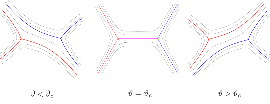
Figure 2: A pop in the triangulation.

Definition 3.27

Let $\vartheta_{c}$ be a critical phase for which a finite $\vartheta_{c}$-trajectory occurs.

1. If the curve connects to two different turning points, the corresponding change in the triangulation shall be called a pop.

2. If the curve is closed and surrounds one singular point, the corresponding change in the triangulation shall be called a flip.

3. If the curve is closed and does not contract to a single, point the corresponding change in the triangulation shall be called a juggle.

GMN show that the coordinates actually don’t change when a pop occurs, so the only relevant jumps for that aspect are the flips and juggles. The property we need now is that although the coordinates jump, a certain $2$-form $\varpi$ that is built out of the derivatives of the $\mathcal{X}$-coordinates is well defined. This works when the jumps do not change $\varpi$, and GMN devote a great effort to proof that this is the case for the most important jumps in [GMN13a]. However there may be jumps for which their argument does no work, so we have to talk about what is rigorously known now. GMN showed that the jumps which correspond to the appearance of a single saddle connection, i. e. pops, are of the right nature and one kind of jumps which corresponds to the appearance of ring domains, i. e. certain juggles, are also fine.

Unfortunately, as GMN themselves note in section 7.6.2 Symplectomorphisms from a BPS vectormultiplet of [GMN13a], a certain phenomenon of the $ca$-triangulation may occur on a Riemann surface $\mathcal{C}$ with genus $g>0$. On such a $\mathcal{C}$ a ring domain may cut off a torus without critical points, i. e. the complement of the ring domain is given by two disjoint subsurfaces, one of which has genus one and does not contain any zeros or poles of $q$. In that case their direct calculation of the jump of the coordinates does not work. Instead they refer to their work on the more general concept of spectral networks in [GMN13] for this case. There they examine differentials which come from a degree $K$ polynomial instead of one with degree $2$ as for our generic differentials here. This leads to a lot of additional language which we can’t properly introduce here, but most importantly they study the jumping behaviour of a certain formal generating function $F$ of formal variables $X_{\gamma}$. The idea is that our $\mathcal{X}$-coordinates can be considered as a special case of these variables and their argument there in section 7.2 Closed loops thus delivers the missing case. But there are some problems with this argument, one being the quite different approach which is not easily translated into the setting here. More importantly though, even if the argument for that case works there may still be a missing case, when one of the boundaries of the ring domains consists of more than one saddle connection.

Now to make these problems precise it is useful to start with the work of T. Bridgeland and I. Smith. In section 5 of [BS15] they first show what kind of ring domains can occur. It turns out that, as stated above, most of these were shown to work in [GMN13a]. The only possibility that has not been rigorously proven is given by the occurrence of a ring domain that cuts off a torus without critical points. Thus we now want to concentrate on those differentials where such a phenomenon does not occur. To formulate this condition it is useful to first introduce the spectrum of a differential.

Definition 3.28

For $q$ a generic quadratic differential, the spectrum of $q$ is the set of all ring domains and all saddle-trajectories for any angle $\vartheta\in[0,2\pi)$.

The elements of the spectrum that may cause problems are ring domains that cut off a torus on which there are no critical points. This case may be pictured accordingly as a torus without any relevant structure and which has a very intricate ring structure attached to one side of it. We hope that the following term captures this picture.

Definition 3.29

Let $q$ be a generic differential. A ring domain that cuts of a torus without any singularities shall be called a signet ring. If the spectrum of $q$ does not contain a signet ring, it shall be called unsealed.

Note that in particular on the sphere (with an arbitrary amount $\geq 4$ of punctures) every generic differential has an unsealed spectrum, so the theory considered here is not vacuous.

For the upcoming discussion we identify the finite $ca$-trajectories with elements of the charge lattice. Following [Nei17] we note that the closure of the lift of a saddle connection for $q$ to the spectral cover $\Sigma^{\prime}_{q}$ is an oriented loop, while the lift of a closed loop to the spectral cover is the union of two oriented loops.

Definition 3.30

Let $q$ be a generic differential and $c$ a finite $ca$-trajectory for $q$. The class in $\Gamma_{q}$ of the corresponding loop (for a saddle connection) or the union of the two loops (for a ring domain) on $\Sigma^{\prime}_{q}$ is called the associated charge.

Note that these associated charges correspond to the elements of $\Gamma_{q}$ that were identified with the edges of a $ca$-triangulation in section 3.3. This identification now allows us to see that saddle connections correspond to specific angles of the $ca$-triangulation. For this we consider the period map $Z_{\gamma}(q^{1/2})=\int_{\gamma}q^{1/2}$, for $\gamma\in\Gamma_{q}$ and $q^{1/2}$ denoting the tautological 1-form on $T^{\ast}\mathcal{C}$.

Lemma 3.31

For a $\vartheta$-saddle connection of $q$ with associated charge $\gamma$ it holds $e^{-i\vartheta}Z_{\gamma}(q^{1/2})\in\mathbb{R}_{+}$.

Proof.

This follows directly from integrating the differential along the $\vartheta$-trajectory. ∎

Thus it is clear, that proportional elements of $\Gamma_{q}$ correspond to the same ray in the $\zeta$-plane. Many of the general properties proven in [BS15] now only hold, when there are no non-proportional elements defining the same $\zeta$-ray. Here we focus notationally on the complement of this set, which are elements of the walls of marginal stability in the work of GMN.

Definition 3.32

A generic quadratic differential with unsealed spectrum shall be called a brick if there exist distinct saddle connections of $q$ such that for their associated elements $\gamma_{1}$ and $\gamma_{2}$ in $\Gamma_{q}$ it holds $\mathbb{Z}\gamma_{1}\neq\mathbb{Z}\gamma_{2}$, but $Z_{\gamma_{1}}(q^{1/2})/Z_{\gamma_{2}}(q^{1/2})\in\mathbb{R}_{+}$.

The connected components of the complement of the set of bricks in the set of generic quadratic differentials with unsealed spectrum shall be called chambers.

The $Z_{\gamma}(q^{1/2})$ for the associated charges $\gamma$ for certain saddle connections of $q$ form local coordinates on the space of quadratic differentials, cf. section 4 in [BS15]. From this it follows that the set of bricks is a countable union of real codimension $1$ submanifolds, from which the name of a wall (and thus of a brick here) arises. From this it follows directly that the chamber-elements are dense in the set of all generic quadratic differentials with unsealed spectrum. In our construction we need to vary a differential without hitting a wall, so we need the following lemma.

Lemma 3.33

Chambers are open in the space of all quadratic differentials.

Proof.

Let $q$ be an element of a chamber. So at any given angle $\vartheta$ at most one element of $\Gamma_{q}$ (up to integer multiples) is the associated charge of some $\vartheta$-trajectory.

For a contradiction suppose that in every neighborhood $U_{t}$ of $q$ there exists a brick $q_{t}$. Thus in every $U_{t}$ there are distinct saddle trajectories $c^{1}_{t}$ and $c^{2}_{t}$. They appear for angles $\vartheta_{t}\in[0,2\pi)$, so we obtain an infinite sequence of angles, which accumulates at some $\vartheta\in[0,2\pi)$ and we pass to a corresponding subsequence converging to $\vartheta$ for $t\to\infty$. As $q$ is not a brick, it follows from Lemma 5.1 in [BS15] that either there is only one finite trajectory or there are two finite trajectories which form the boundary of a ring domain.

We first consider the case of a single trajectory and distinguish two cases. First we suppose that there is no $t_{0}$ such that for all $t>t_{0}$ $\vartheta_{t}=\vartheta$. Thus near $q$ there are at least two $ca$-trajectories for angles arbitrarily close to $\vartheta$. Now since $q$ has only one finite $\vartheta$-trajectory it follows from Proposition 5.5 in [BS15] that in a sufficiently small neighborhood of $q$ there can’t be a $\vartheta+\epsilon$-trajectory for small enough $\epsilon\neq 0$. So this case cannot occur.

On the other hand, if such a $t_{0}$ exists, we obtain a sequence of differentials $q_{t}$ near $q$ which all have at least two distinct $\vartheta$-trajectories. But, as of Lemma 5.2. in [BS15] the subset of differentials with only one $\vartheta$-trajectory is open in the space of all quadratic differentials. So this case also cannot occur.

For the case of a ring domain the analogous statements follow from the same results in [BS15]. Thus a sequence of wall-elements can only accumulate at wall-elements, so the subset of non-wall elements is open.

∎

Before moving on, let us consider the spectrum in some more detail. The use of some additional technique of [BS15] will allow us to loosen the restriction of the differential in Proposition 8.3 quite a bit. In the definition of the spectrum we did not count the infinitely many closed $\vartheta$-trajectories which sweep out a ring domain as separate elements, although they are finite $ca$-trajectories. The reason for this is the fact that the ring domain as a whole occurs at some specific angle $\vartheta_{c}$ and leads to a (collective) jump in the $ca$-triangulation at $\vartheta_{c}$, as was shown in [GMN13a]. Additionally all these closed trajectories have the same lift on the spectral cover as they are homotopic. But the existence of a ring domain still does lead to an infinite spectrum, because near $\vartheta_{c}$ an infinite sequence of saddle connections may occur. These saddle connections lead to distinct jumps of the triangulation and accumulate at $\vartheta_{c}$. So it seems quite natural for the spectrum of a generic differential to be infinite, but the way in which a generic differential with unsealed spectrum is infinite is well understood. Indeed, infinitely many saddle connections occur only near ring domains (cf. section 5.3. in [Tah17]) and in the case of an unsealed spectrum their behaviour near such ring domains is completely described in [GMN13a]. This also implies that ring domains do not accumulate, as they would have to accumulate near a ring domain, which is not possible as of the analysis in [GMN13a]. Therefore we have the following observation:

Lemma 3.34

An unsealed spectrum has at most finitely many ring domains.

The analysis in [GMN13a] tells us how to calculate the jumps for ring domains and their corresponding infinite amount of saddle connections. With this lemma it is now clear, that there can only be finitely many additional jumps from single saddle connections and thus all jumps can be calculated. Otherwise, if there were an infinite sequence of ring domains, there would be technical difficulties in defining the right order for the occurring jumps. But for unsealed spectra we don’t have to worry about this.

We will come back to this property of only having finitely many accumulation points later on, when considering the associated Riemann-Hilbert problem. Here the only condition which really seems to shorten the applicability of our results is the existence of signet rings, but there is a way to lessen their impact, which we will describe now.

Remark 3.35

Suppose $q$ has a spectrum that is at first not unsealed. Thus Proposition 8.3 does not work as there is a ring domain cutting off a torus without singularities. In those cases, as was shown in [BS15], the ring domain has boundaries which are made up of some number of saddle connections and are thus strongly non-degenerate in the terminology of Bridgeland and Smith. It is then shown that such strongly non-degenerate ring domains can be removed without altering the genus of the surface or the differential outside of the ring domain. This process is called ring-shrinking and can roughly be considered as compressing the ring domain into a single closed curve.

After the ring shrinking the jump of the former ring domain becomes one of the jumps that was shown to be fine. If there are only finitely many signet rings it should then be possible to obtain an unsealed spectrum after finitely many ring shrinking moves, so there is no danger of shrinking the surfaces to a point or changing the topology in any other way, which could broaden the applicability of the theory presented here a lot.

However, one has to show that the ring shrinking, which eliminates a ring domain for one specific $\vartheta_{c}$ does not produce another ring domain at some other angle. Additionally, we are interested in properties for the moduli space for varying differentials. Therefore we would need the ring shrinking to work uniformly in at least some open subset of the Hitchin base. But varying the differential in the wrong direction might exactly reproduce the ring domain we just got rid of, cf. section 5.9 Juggles in [BS15]. Finally, it seems reasonable that there are only finitely many signet rings in the spectrum of any given generic differential, but this is not rigorously proven yet.

Further explorations of these phenomenons would be very useful to obtain the most general setting for our theory. Additionally, as we explained above, the jumps corresponding to the shrunken ring domains may actually also be such that the holomorphic symplectic form $\varpi$ is well defined, and it may be possible to obtain a proof for those jumps from the arguments given in [GMN13]. Such a proof, written in terms of the $\mathcal{X}$-coordinates, would be quite useful to obtain more information about the actual limits of this construction. But for now and for the rest of this section we will be content with the demand for $q$ to have an unsealed spectrum.

4 Local description of the solutions to Hitchin’s equations

In this section we calculate local forms of all the objects we need in a way that fits the aforementioned construction of the canonical coordinates. We start by explaining the fundamental result of [Fre+20] in subsection 4.1 and then build a standard frame over certain subsets of the standard quadrilaterals that were introduced in the previous section. This will then allow us to calculate local forms of the Harmonic metric, Higgs field and Chern connection in subsection 4.2 that are suited for the construction.

4.1 Construction of the standard frame

Our construction of the metric will mostly be done via local data of the solutions of Hitchin’s equation, for which we build on the theory of limiting configurations developed in [Fre+20]. For the rest of this section we fix a stable $SL(2,\mathbb{C})$-Higgs bundle $(\mathcal{E},\Phi)$ in the regular locus $\mathcal{M}^{\prime}$ of $\mathcal{M}$ s. t. $-q\mathrel{\mathop{\mathchar 58\relax}}=\det\Phi$ has only simple zeroes. FMSW constructed solutions $h_{R}$ of the $R$-rescaled Hitchin equation

$$F^{\bot}_{A_{h_{R}}}+R^{2}\left[\Phi,\Phi^{\ast_{h_{R}}}\right]=0$$

for large $R\in\mathbb{R}$. The idea behind this rescaling is, that for large $R$, corresponding to large Higgs fields, Hitchin’s equation would decouple leading to a much simpler set of equations that can be solved explicitly. The decoupled equations are the limiting equations

$$F^{\bot}_{A_{h_{\infty}}}=0,\quad\text{and}\quad\left[\Phi,\Phi^{\ast_{h_{\infty}}}\right]=0$$

and the harmonic metric $h_{\infty}$ is called the limiting metric, which corresponds to the limiting pair $(A_{\infty},\Phi_{\infty})$. Local forms near zeroes and poles of these objects are given in [Fre+20] which were then glued together to create an approximate solution $h_{\text{app}}$ of the true Hitchin equation. The foundational result for our work that they obtained is that for large enough $R$ there exists a gauge transformation that transforms the approximate solution into a true solution. We paraphrase the result here which is found as Theorem 6.2. in [Fre+20].

Theorem 4.1

There exists $R_{0}>1$ such that for every $R\geq R_{0}$ there exists an $h_{0}$-Hermitian endomorphism $\gamma_{R}$, s. t. $g\cdot h_{\text{app}}$ for $g=\exp(\gamma)$ is a true solution of the $R$-rescaled Hitchin equation. Furthermore $\gamma_{R}$ is unique amongst endomorphisms of small norm.

Not only did FMSW show the existence of these approximate solutions and the correction mechanism. They also showed that the transformation is exponentially suppressed in $R$. These results are foundational for the work at hand as they seem to imply that other objects that were constructed with the help of these solutions might as well inherit the structure of an explicit approximate solution plus some correctional term that is exponentially suppressed. In order to really make use of the results one would however need a way of implementing it in an appropriate construction of e. g. the hyperkähler metric of $\mathcal{M}$. As it turns out, the proposed construction by GMN allows for precisely such an implementation as we want to show here.

For all of this to work we will have to make heavy use of the explicitly known local forms of all the moving parts which will later be the ingredients of our flat connection for the GMN construction. So our goal here is to write the ingredients of the twistor connection as a diagonal leading term plus some remainder or ”error”-term which behaves in a certain way when going into a parabolic point, as well as when considering large $R$.

In the following $z$ will always be a local coordinate on $\mathcal{C}$ with $r\mathrel{\mathop{\mathchar 58\relax}}=|z|$ in any coordinate centered around a parabolic point. We start by considering the local frame $(e_{1},e_{2})$ in which we would like to work. We are interested in frames that are adjusted to the Higgs field $\Phi=\varphi dz$, so that $\varphi$ has diagonal form

$$\varphi=\begin{pmatrix}f^{1/2}&0\\ 0&-f^{1/2}\end{pmatrix}$$

for some square root $f^{1/2}$ of $f=-\det\varphi$.

Lemma 4.2

Let $(\mathcal{E},\Phi)$ be a parabolic Higgs bundle with local Higgs field $\Phi=\varphi dz$ with determinant $\det\Phi=\det\varphi dz^{2}=-fdz^{2}$. In any gauge in which $\varphi$ is diagonal, the holomorphic structure splits, i. e. is also represented by a diagonal matrix.

Proof.

Assume $\varphi$ to be diagonal, i. e. of the form

$$\varphi=\begin{pmatrix}f^{1/2}&0\\ 0&-f^{1/2}\end{pmatrix}$$

for some square root $f^{1/2}$ of $f$. We now write the holomorphic structure locally as

$$\overline{\partial}_{E}=\overline{\partial}+A_{\overline{z}}d\overline{z}=\overline{\partial}+\begin{pmatrix}\overline{a_{1}}&\overline{a_{2}}\\ \overline{a_{3}}&\overline{a_{4}}\end{pmatrix}d\overline{z},$$

where $\overline{\partial}$ is the trivial holomorphic structure induced by the coordinate $z$. As $(\Phi,\overline{\partial}_{E})$ is a Higgs bundle it holds $\overline{\partial}_{E}\Phi=0$, i. e.

$$0=\partial_{\overline{z}}\varphi+[A_{\overline{z}},\varphi].$$

In some more detail: Let $s$ be any section, then it holds:

$$\begin{split}0&=(\overline{\partial}_{E}\varphi)s=\overline{\partial}_{E}(\varphi s)-\varphi\overline{\partial}_{E}(s)=\partial_{\overline{z}}(\varphi s)+A_{\overline{z}}\varphi s-\varphi\partial_{\overline{z}}s-\varphi A_{\overline{z}}\\ &=\begin{pmatrix}\partial_{\overline{z}}(f^{1/2}s_{1})\\ -\partial_{\overline{z}}(f^{1/2}s_{2})\end{pmatrix}+\begin{pmatrix}\overline{a_{1}}&\overline{a_{2}}\\ \overline{a_{3}}&\overline{a_{4}}\end{pmatrix}\begin{pmatrix}f^{1/2}&0\\ 0&-f^{1/2}\end{pmatrix}s\\ &-\begin{pmatrix}f^{1/2}&0\\ 0&-f^{1/2}\end{pmatrix}\begin{pmatrix}\partial_{\overline{z}}s_{1}\\ \partial_{\overline{z}}s_{2}\end{pmatrix}-\begin{pmatrix}f^{1/2}&0\\ 0&-f^{1/2}\end{pmatrix}\begin{pmatrix}\overline{a_{1}}&\overline{a_{2}}\\ \overline{a_{3}}&\overline{a_{4}}\end{pmatrix}s\\ &=\begin{pmatrix}(\partial_{\overline{z}}f^{1/2})s_{1}\\ -(\partial_{\overline{z}}f^{1/2})s_{2}\end{pmatrix}+\begin{pmatrix}-2\overline{a_{2}}f^{1/2}s_{2}\\ 2\overline{a_{3}}f^{1/2}s_{1}\end{pmatrix}.\end{split}$$

Plugging in $s=(1,0)$ and $s=(0,1)$ we obtain $\overline{a_{2}}=\overline{a_{3}}=0$. ∎

We now introduce the standard neighborhood on which most of the following local calculations take place, for which we recall the $ca$-triangulations of section 3.1. We take $-q=\det\Phi$ and consider any generic angle $\vartheta$ i. e. the corresponding $\vartheta$-triangulation has no finite $\vartheta$-trajectories. For any edge of the triangulation we consider the two triangles that share this edge. They form a quadrilateral $Q$ bounded by four different $\vartheta$-trajectories inside some bigger open patch $U\subset C$. The trajectories connect four different weakly parabolic points and inside the quadrilateral are two (distinct) zeroes of $\det\phi$ (cf. figure 3).

Now we may take a simple closed curve in $U$ that touches all four weakly parabolic points and whose interior $O\subset U$ contains all four $\vartheta$- trajectories that bound the quadrilateral. Inside $O$ we may also take a simple closed curve whose interior $\widetilde{O}\subset O$ contains both zeroes of $\det\Phi$. Then $S\mathrel{\mathop{\mathchar 58\relax}}=O\setminus\widetilde{O}$ is homeomorphic to an annulus, does not contain the zeroes or poles of $\det\Phi$, but does contain the $\vartheta$-trajectories that form the boundary of the quadrilateral.

Definition 4.3

Let $q$ be a generic differential and $\vartheta$ a generic angle. Any quadrilateral obtained from two triangles that share an edge shall be called a standard quadrilateral and any domain $S\in\mathcal{C}$ constructed in the way described above out of $Q$ shall be called a standard annulus of the triangulation. In particular such a domain does not contain any of the critical points of $-q$ and any simple closed curve in $S$ surrounds either no or two zeroes of $-q$ in $Q$.

Note that if we vary $-q=\det\Phi$ or the the angle $\vartheta$ of the $ca$-triangulation the poles, zeroes and curves may vary. If we do this continuously depending on some parameter $\epsilon$ all the parts depend continuously on $-q$ and $\vartheta$ (except for the critical values for $\vartheta$). Thus it is always possible to choose a domain that is a standard annulus for all $\epsilon$ in some interval.

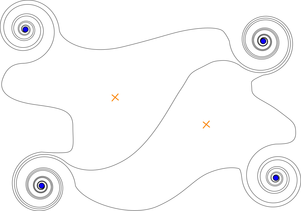
Figure 3: A standard quadrilateral consisting of two triangles that share a common $ca$-trajectory. The blue dots represent weakly parabolic points and the orange crosses represent zeroes of $-q$.

Thus defined we now establish that a standard annulus is a good working environment for our case. For the rest of this section a Higgs field $\Phi$ with determinant $-q$ a generic differential and a generic angle $\vartheta$ shall be fixed.

Lemma 4.4

Let $\Phi=\varphi dz$ be a Higgs field on a standard quadrilateral $Q$ standard annulus $S$. Then there exists a (holomorphic) frame on $S$ in which $\varphi$ is diagonal.

Proof.

Let $c\mathrel{\mathop{\mathchar 58\relax}}[a,b]\rightarrow C$ be a simple closed curve in $S$. Then $c$ is homotopic to a point or $c$ surrounds the two zeroes of $-q=\det\Phi$ in $Q$. As $c$ can’t surround only one zero a standard result of complex analysis shows that a well defined square root $q^{1/2}$ on the whole annulus can be chosen. (This corresponds to choosing one sheet of the double cover by the spectral curve.) In every point $x$ in $S$ the eigenvalues $\pm q^{1/2}(x)$ are distinct and as the square root is well defined they don’t interchange. Thus we obtain two disjoint eigenspaces $E_{x_{+}}$, $E_{x_{-}}$ in every point $x$ which form two distinct line bundles $E_{+}$, $E_{-}$ on $S$. Locally we can thus choose a frame in which $\varphi$ is diagonal. As $\overline{\partial}_{E}(\Phi)=0$, the diagonality of $\varphi$ implies as of Lemma 4.2 that the holomorphic structure $\overline{\partial}_{E}$ is diagonal, i. e. splits into a holomorphic structure on each line bundle. Thus $E_{+}$ and $E_{-}$ are holomorphic line bundles. Since they are defined on the non-compact Riemann surface $S$ they have to be holomorphically trivial (see [For81] p. 229). Thus we can choose some non-vanishing sections over $S$ with respect to which $\varphi$ will be diagonal on all of $S$. ∎

In the following we compute the local forms of the Higgs field, its adjoint and the Chern connection of the holomorphic structure w. r. t. the Hermitian metric $h_{R}$ on a standard annulus or subsets thereof. For these computations we first need to collect the information on $h_{R}$ from [Fre+20] which for simplicity we will just call $h\mathrel{\mathop{\mathchar 58\relax}}=h_{R}$ for the rest of the section keeping in mind that all the constructions are considered for large enough $R$. So we start by choosing the approximate metric $h_{0}$, which was defined in [Fre+20] as $h_{R}^{app}$, as our background metric on $E$. In [Fre+20] it is shown for $\text{pdeg}(\mathcal{E})=0$ that $h_{0}=h_{R}^{app}$ is adapted to the parabolic structure for weakly parabolic bundles and induces the fixed flat Hermitian structure on Det$E$. The metric is defined in such a way that away from zeroes of $q$ the eigenspaces of $\Phi$ are orthogonal, thus $\Phi$ is represented by a diagonal matrix in any frame given by sections of the eigenspaces such as the frame constructed above in which $\varphi$ is diagonal. In [Fre+20] we also find local forms for $h_{0}$ near all the different exceptional points for $q$. Here we only note the holomorphic frame above can be rescaled into a frame $F^{\ast}\mathrel{\mathop{\mathchar 58\relax}}=(e^{\ast}_{1},e^{\ast}_{2})$ on $S$ s. t. the matrix $H_{0}$ representing $h_{0}$ has the following form near the (double) poles $p_{i}$ of $q$:

$$H_{0}=Q\begin{pmatrix}|z|^{2\alpha_{1}(p)}&0\\ 0&|z|^{2\alpha_{2}(p)}\end{pmatrix}.$$

Here $\alpha_{1},\alpha_{2}$ are the parabolic weights and $Q$ is some locally defined and non-vanishing smooth function, completely determined by $h_{\text{Det}\mathcal{E}}$, the choice of holomorphic section of Det$\mathcal{E}$ and coordinate $z$. Note that this metric coincides with $h_{\infty}$ in [Fre+20]. For our calculations it is convenient to change to an $h_{0}$-unitary frame near the $p_{i}$, so we define

$$\tilde{e_{1}}=\frac{e^{\ast}_{1}}{Q^{1/2}|z|^{\alpha_{1}}},\quad\tilde{e}_{2}=\frac{e^{\ast}_{2}}{Q^{1/2}|z|^{\alpha_{2}}}.$$

Then it holds $H_{0}=E_{2}$ in the frame $(\tilde{e}_{1},\tilde{e}_{2})$ near the $p_{i}$.

Away from poles or zeros of det$\Phi$ the metric is still diagonal in any holomorphic frame and has the general form

$$H_{0}=\begin{pmatrix}f&0\\ 0&g\end{pmatrix}$$

for some non-vanishing functions $f,g$. Thus via some diagonal transformation we obtain the local form $H_{0}=E_{2}$ everywhere away from zeros of det$\Phi$ in this frame $\tilde{F}$. Note that scaling away $Q$ is not strictly necessary but rather simplifies a lot of the following expression. It is also convenient to make another ($h_{0}$-unitary) transformation to obtain a certain form for the matrix-coefficients representing the holomorphic structure $\overline{\partial}_{E}$.

Lemma 4.5

On the standard annulus $S$ there exists an $h_{0}$-unitary frame $F$ in which the Higgs field is diagonal as is the matrix representing the holomorphic structure $\overline{\partial}_{E}$. Additionally the Chern connection w. r. t. $h_{0}$ is represented by a $1$-form valued matrix $C$ with $dC=0$ for the standard differential $d=\partial+\overline{\partial}$.

Proof.

Let $\tilde{F}$ be the aforementioned $h_{0}$-unitary frame. In this frame the Higgs field is diagonal and as of Lemma 4.2 the holomorphic structure is of the form

$$\overline{\partial}_{E}=\overline{\partial}+\begin{pmatrix}\tilde{a}_{1}&0\\ 0&\tilde{a}_{2}\end{pmatrix}d\overline{z},$$

for some differentiable functions $\tilde{a}_{1}$ and $\tilde{a}_{2}$. Again we use the fact that the standard annulus is a non-compact Riemann surface and thus there exist functions $A_{1}$ and $A_{2}$, s. t. $\overline{\partial}A_{1}=\tilde{a}_{1}d\overline{z}$ and $\overline{\partial}A_{2}=\tilde{a}_{2}d\overline{z}$ (see [For81], Theorem 25.6). With $T_{1}\mathrel{\mathop{\mathchar 58\relax}}=-i\text{Im}(A_{1})$ and $T_{2}\mathrel{\mathop{\mathchar 58\relax}}=-i\text{Im}(A_{2})$ define the (unitary) transition matrix

$$g\mathrel{\mathop{\mathchar 58\relax}}=\begin{pmatrix}e^{T_{1}}&0\\ 0&e^{T_{2}}\end{pmatrix}.$$

and let $F$ denote the frame obtained from this change of basis. It is still $h_{0}$-unitary, so $H_{0}=E_{2}$ while the holomorphic structure has the form

$$\overline{\partial}_{E}=\overline{\partial}+A\mathrel{\mathop{\mathchar 58\relax}}=\overline{\partial}+\begin{pmatrix}\tilde{a}_{1}&0\\ 0&\tilde{a}_{2}\end{pmatrix}d\overline{z}+\begin{pmatrix}T_{1}&0\\ 0&T_{2}\end{pmatrix}d\overline{z}.$$

As the frame is unitary, the matrix representing the Chern connection w. r. t. $h_{0}$ is simply $C\mathrel{\mathop{\mathchar 58\relax}}=A-\overline{A}^{t}$. A straight forward calculation now shows that $dC=0$. ∎

This specific choice of frame will be useful in section 6.1 as it allows for a simple construction of the leading terms of the Fock-Goncharov-coordinates. In almost all of the following calculations we will work in this frame, so we denote it as our standard.

Definition 4.6

The $h_{0}$-unitary frame $F$ constructed in Lemma 4.5 on a standard annulus $S$ shall be called the standard frame on $S$.

4.2 Local forms of Higgs pairs

We now want to describe the harmonic metric $h$ in the $h_{0}$-unitary frame $F$, which as of [Fre+20] we obtain for large enough $R$ by the action of a gauge transformation $g$ acting on $h_{0}$ via $h=g\cdot h_{0}(v,w)=h_{0}(gv,gw)$. In the chosen gauge we have $h_{0}(v,w)=\overline{v}^{t}H_{0}w$ and thus

$$g\cdot h_{0}(v,w)=\overline{gv}^{t}H_{0}gw=\overline{v}^{t}\overline{g}^{t}H_{0}gw=\overline{v}^{t}\overline{g}^{t}gw.$$

Let $H$ be the matrix representing $h$ in this gauge, i. e. $h(v,w)=\overline{v}^{t}Hw$. Then, as $h=g\cdot h_{0}$ we obtain $H=\overline{g}^{t}H_{0}g=\overline{g}^{t}g$. Now from [Fre+20] we have $g=\exp(\gamma)$ for $\gamma$ $h_{0}$-Hermitian and traceless, so $g$ is also $h_{0}$-Hermitian and has determinant $1$. We write $g$ accordingly as

$$g=\mathrel{\mathop{\mathchar 58\relax}}\begin{pmatrix}a&b\\ \overline{b}&d\end{pmatrix}$$

with $a,d$ real-valued functions on $S$ and $ad-|b|^{2}=1$. The behavior of the entries of $g$ is determined by the behavior of the entries of $\gamma$ in the following way:

Lemma 4.7

Let $\gamma$ be tracefree and $h_{0}$-hermitian with $D\mathrel{\mathop{\mathchar 58\relax}}=\det(\gamma)$. Then

$$g=\exp(\gamma)=\cosh(\sqrt{-D})E_{2}+\tfrac{\sinh(\sqrt{-D})}{\sqrt{-D}}\gamma.$$

Proof.

This is a standard calculation: As $\gamma$ is tracefree and $h_{0}$-hermitian we may write it as

$$\gamma=\begin{pmatrix}l&o\\ \overline{o}&-l\end{pmatrix}$$

for some real valued function $l$ and complex valued function $o$. Thus $D\mathrel{\mathop{\mathchar 58\relax}}=\det(\gamma)=-l^{2}-|o|^{2}\leq 0$ and $\gamma^{2}=-DE_{2}$. From this we obtain

$$\begin{split}\exp(\gamma)&=\sum_{k=0}^{\infty}\frac{\gamma^{k}}{k!}=\sum_{k=0}^{\infty}\frac{\gamma^{2k}}{(2k)!}+\sum_{k=0}^{\infty}\frac{\gamma^{2k+1}}{(2k+1)!}\\ &=\sum_{k=0}^{\infty}\frac{(-D)^{k}E_{2}}{(2k)!}+\sum_{k=0}^{\infty}\frac{(-D)^{k}\gamma}{(2k+1)!}=\sum_{k=0}^{\infty}\frac{\sqrt{-D}^{2k}}{(2k)!}E_{2}+\sum_{k=0}^{\infty}\frac{\sqrt{-D}^{2k}}{(2k+1)!}\gamma\\ &=\sum_{k=0}^{\infty}\frac{\sqrt{-D}^{2k}}{(2k)!}E_{2}+\frac{1}{\sqrt{-D}}\sum_{k=0}^{\infty}\frac{\sqrt{-D}^{2k+1}}{(2k+1)!}\gamma=\cosh(\sqrt{-D})E_{2}+\frac{\sinh(\sqrt{-D})}{\sqrt{-D}}\gamma.\end{split}$$

∎

This Lemma relates the properties of $\gamma$ to the properties of $g$, from which we obtain the necessary information about $H$ as we have:

$$H=\overline{g}^{t}g=\begin{pmatrix}a^{2}+|b|^{2}&(a+d)b\\ (a+d)\overline{b}&d^{2}+|b|^{2}\end{pmatrix}=\mathrel{\mathop{\mathchar 58\relax}}\begin{pmatrix}\alpha&\beta\\ \overline{\beta}&\delta\end{pmatrix}.$$

We will use the following observation in some calculations later on:

Lemma 4.8

In the standard frame $F$ on the standard annulus the matrix $H$ that represents the Hermitian harmonic metric $h$ has determinant $1$.

Proof.

This follows readily from the discussion of the local form above as $g$ has determinant $1$. ∎

We are interested in the decaying behavior of the entries of $H$ near weakly parabolic points and we will also need the behavior of the entries of $H^{-1}\partial H$. Using 4.8 we obtain

$$H^{-1}\partial H=\begin{pmatrix}\delta\partial\alpha-\beta\partial\overline{\beta}&\partial(\beta\delta)\\ -\partial(\alpha\overline{\beta})&-(\delta\partial\alpha-\beta\partial\overline{\beta})\end{pmatrix}=\mathrel{\mathop{\mathchar 58\relax}}\begin{pmatrix}h_{1}&h_{2}\\ h_{3}&-h_{1}\end{pmatrix}.$$

We now obtain all the information from the properties of $\gamma$ which were established in [Fre+20].

Lemma 4.9

There exists a local coordinate $z$ centered around any weakly parabolic point, such that the following asymptotics hold for the functions defined above (with $r\mathrel{\mathop{\mathchar 58\relax}}=|z|$) for some $\mu>0$ and all $1\leq i\leq 3$:

$$a,d,\alpha,\delta=O(1),\quad b,\beta=O(r^{\mu}),\quad h_{i}=O(r^{\mu-1}).$$

Furthermore, if $\epsilon$ denotes a $C^{2}$-coordinate of $\mathcal{M}^{\prime}$, then the derivatives w. r. t. $\epsilon$ exist and have the same asymptotics:

$$\partial_{\epsilon}a,\enspace\partial_{\epsilon}d,\enspace\partial_{\epsilon}\alpha,\enspace\partial_{\epsilon}\delta =O(1), \quad\partial_{\epsilon}b,\enspace\partial_{\epsilon}\beta\enspace =O(r^{\mu}),$$

$$\partial^{2}_{\epsilon}a,\enspace\partial^{2}_{\epsilon}d,\enspace\partial^{2}_{\epsilon}\alpha,\enspace\partial^{2}_{\epsilon}\delta =O(1), \quad\partial^{2}_{\epsilon}b,\enspace\partial^{2}_{\epsilon}\beta =O(r^{\mu}),$$

$$\partial_{\epsilon}h_{i},\partial^{2}_{\epsilon}h_{i} =O(r^{\mu-1}).$$

Additionally there exist constants $C,\nu>0$ s. t.

$$|r^{-\mu}b|,|r^{-\mu}\beta|,|r^{1-\mu}h_{i}|\leq Ce^{-\nu R}\quad\text{and}\quad|r^{1-\mu}\partial_{\epsilon}h_{i}|\leq Ce^{-\nu R}$$

for large enough $R$.

Proof.

One important result in [Fre+20] is that the gauge transformation $\gamma$ that transforms the approximate solution of the Hitchin equations lies in the Friedrichs domain $\mathcal{D}_{\text{Fr}}^{0,\alpha}(\nu)$. In particular $\gamma$ has a partial expansion in (non-negative) powers of $r$, where the first term is a constant diagonal matrix. This gives the first asymptotics for the entries of $\gamma$ by definition of the domain .

The $\epsilon$-differentiability for the entries of $\gamma$ follows from an appropriate enhancement of the application of the inverse function theorem that shows the existence of $\gamma$. The asymptotics for the $\epsilon$-derivatives follow readily as the $r$-dependence in $\mathcal{D}_{\text{Fr}}^{0,\alpha}(\nu)$ is independent of the $\epsilon$-dependence.

Finally the exponential suppression is also an explicit part of the result of [Fre+20].

This shows all the conditions for the entries of $\gamma$. As $\det(\gamma)$ is well defined and non-zero on the standard annulus it follows from Lemma 4.7 that the properties also hold for the entries of $g$ and correspondingly for $H$. The properties for the $h_{i}$ follow in the same way, using the fact, that the first two polar derivatives also lie in the corresponding domain as shown in [Fre+20]. ∎

With this information we can now calculate the rest of the protagonists of our construction.

Corollary 4.10

In the standard frame $F$ on the standard annulus $S$ the adjoint Higgs field (w. r. t. the harmonic metric $h$) can be written as

$$\Phi^{\ast_{h}}=\left(\overline{f^{1/2}}\sigma^{3}+\overline{f^{1/2}}\varphi^{er}\right)d\overline{z}$$

for $\varphi^{er}$ some traceless matrix whose entries are $O(r^{\mu})$ for some $\mu>0$ near any weakly parabolic point.

Proof.

Using 4.8 the adjoint Higgs field $\Phi^{\ast_{h}}=\varphi^{\ast_{h}}d\overline{z}$ is calculated as

$$\begin{split}\varphi^{\ast_{h}}&=H^{-1}\overline{\varphi}^{t}H=\begin{pmatrix}\delta&-\beta\\ -\overline{\beta}&\alpha\end{pmatrix}\begin{pmatrix}\overline{f^{1/2}}&0\\ 0&-\overline{f^{1/2}}\end{pmatrix}\begin{pmatrix}\alpha&\beta\\ \overline{\beta}&\delta\end{pmatrix}\\ &=\overline{f^{1/2}}\begin{pmatrix}\alpha\delta+|\beta|^{2}&2\delta\beta\\ -2\alpha\overline{\beta}&-\alpha\delta-|\beta|^{2}\end{pmatrix}=\begin{pmatrix}\overline{f^{1/2}}&0\\ 0&-\overline{f^{1/2}}\end{pmatrix}+2\overline{f^{1/2}}\begin{pmatrix}|\beta|^{2}&\delta\beta\\ -\alpha\overline{\beta}&-|\beta|^{2}\end{pmatrix}.\end{split}$$

Thus the adjoint Higgs field consists of a diagonal leading term plus a remainder whose entries are all at least linear in $|\beta|$. As of Lemma 4.9 the remainder behaves in specified way. ∎

The final ingredient is the Chern connection for $\overline{\partial}_{E}$ for the harmonic metric $h$, which we also want to describe with a ”simple” leading term and a ”small” remainder.

Corollary 4.11

In the frame standard frame $F$ on the standard annulus $S$ the Chern connection $A$ (w. r. t. the harmonic metric $h$) of $\overline{\partial}$ can be expressed as

$$A=d+\begin{pmatrix}\overline{a_{1}}d\overline{z}-a_{1}dz&0\\ 0&\overline{a_{2}}d\overline{z}-a_{2}dz\end{pmatrix}+(a_{2}-a_{1})A^{er}dz+H^{-1}\partial H,$$

where $d=\partial+\overline{\partial}$ is the standard differential and $A^{er}$ is some traceless matrix whose entries are $O(r^{\mu})$ for some $\mu>0$ near any parabolic point.

Proof.

By construction the holomorphic structure in the standard frame $F$ has the form

$$\overline{\partial}_{E}=\overline{\partial}+A_{\overline{z}}=\overline{\partial}+\begin{pmatrix}\overline{a_{1}}&0\\ 0&\overline{a_{2}}\end{pmatrix}d\overline{z},$$

for some function $a_{1},a_{2}$. A direct calculation using that $H$ is $h_{0}$-hermitian shows that the Chern connection $d_{A}=d+A$ with respect to $h$ is given as

$$d+A=d+A_{\overline{z}}d\overline{z}-A_{\overline{z}}^{\ast_{h}}dz+H^{-1}\partial H.$$

So we need to calculate $A_{\overline{z}}^{\ast_{h}}$, which becomes

$$\begin{split}A_{\overline{z}}^{\ast_{h}}&=H^{-1}\overline{A_{\overline{z}}}H=\begin{pmatrix}\delta&-\beta\\ -\overline{\beta}&\alpha\end{pmatrix}\begin{pmatrix}a_{1}&0\\ 0&a_{2}\end{pmatrix}\begin{pmatrix}\alpha&\beta\\ \overline{\beta}&\delta\end{pmatrix}dz\\ &=\begin{pmatrix}a_{1}\alpha\delta-a_{2}|\beta|^{2}&(a_{1}-a_{2})\delta\beta\\ -(a_{1}-a_{2})\alpha\overline{\beta}&a_{2}\alpha\delta-a_{1}|\beta|^{2}\end{pmatrix}dz=\begin{pmatrix}a_{1}&0\\ 0&a_{2}\end{pmatrix}+(a_{1}-a_{2})\begin{pmatrix}|\beta|^{2}&\delta\beta\\ -\alpha\overline{\beta}&-|\beta|^{2}\end{pmatrix}dz,\end{split}$$

where we used 4.8. Thus the whole connection becomes

$$d_{A}=d+\begin{pmatrix}\overline{a_{1}}d\overline{z}-a_{1}dz&0\\ 0&\overline{a_{2}}d\overline{z}-a_{2}dz\end{pmatrix}+(a_{2}-a_{1})\begin{pmatrix}|\beta|^{2}&\delta\beta\\ -\alpha\overline{\beta}&-|\beta|^{2}\end{pmatrix}dz+H^{-1}\partial H.$$

Again the structure is that of a diagonal leading term and an remainder term whose entries depend at least linearly on $|\beta|$ and thus have the specified decaying behavior. ∎

Note that the factor $H^{-1}\partial H$ should also be considered as part of the remainder term as it is part of the deviation from the diagonal leading term. It consists only of data coming from the harmonic metric and thus only depends indirectly (via the solution of Hitchin’s equation) on the Higgs field and holomorphic structure. Most importantly it also has the pole-structure we need: In 4.9 it was shown that the $h_{i}$ are $O(r^{\mu-1})$ while $b$ and $\beta$ are $O(r^{\mu})$. This matches in the emerging formula in section 6, as the other remainder terms for the Higgs field and the Chern connection obtain a pole of order $1$ through $\overline{f^{1/2}}$ and $a_{2}-a_{1}$.

Remark 4.12

We have obtained the structure of a leading term plus a ”small” remainder for both the data from the Higgs field $\Phi$ and from the connection $A$ which will together form the connection matrix for a connection $\nabla$ in the next section. The remainder $\overline{f^{1/2}}\varphi^{er}d\overline{z}+(a_{2}-a_{1})A^{er}dz+H^{-1}\partial H$ of this matrix is traceless which is seen directly for the parts $\varphi^{er}$ and $A^{er}$ and follows for $H^{-1}\partial H$ by a simple calculation from the fact that $H$ has constant determinant.

As $\varphi$ is traceless by definition of our moduli space the only part that isn’t comes from the leading part of the Chern connection $A$. One could arrange for this part to also be traceless by shifting the parabolic weights, which simplifies some of the following calculations and which is actually the form [GMN13a] use. We don’t do this here as we follow the set-up of [Fre+20]. Additionally this shows that no specific choice of weights is necessary. However, thinking of $A$ as traceless leads to more convenient formulas and our treatment actually shows that one can think of these objects in this way without loosing any important structure.

We have now obtained all of the data that we need for the following constructions and would like to compute the Darboux coordinate system as described in section 3.2. That is, we can construct $\nabla(\zeta)=\tfrac{R}{\zeta}\Phi+A+R\zeta\Phi^{\ast_{h}}$ for $\zeta\in\mathbb{C}^{\times}$ and try to solve the flatness equation $\nabla(\zeta)v=0$, where we observe the aforementioned structure of a diagonal leading term and a ”small” remainder. As it turns out it is possible to solve this equation along $ca$-curves but to do so in a proper way, one needs some non-standard theory for singular ODEs which we will develop in the next section.

5 Initial value problems at infinity

The crucial ingredient in our construction are the so called ”small flat sections” obeying the flatness equation of a connection build out of a Higgs pair. This connection, when trivialized along a $ca$-curve, becomes a $2\times 2$ non-autonomous linear ODE. The small flat sections are supposed to be solutions of this ODE that decay in a certain way as $t\rightarrow\infty$. Thus we want to solve an ODE uniquely (up to a complex multiple) be demanding a certain behaviour at $\infty$, which differs substantially from the usual boundary value problems where the boundary value is given at a finite time. This becomes a problem as we want to differentiate the solutions with respect to a parameter and the standard theory requires a boundary value or initial value at some finite time. It turns out, that to solve this problem the theory of Volterra integral equations is helpful, as they encode the boundary value in an explicit term of the equation. This allows for a rigorous definition of the small flat section and furthermore exploration of their differentiable behavior. Therefore we will use this section to study these types of equations. We will completely ignore the origin of the problem in the theory of Higgs bundles in this section and instead develop the theory in its own purely analytical setting, which may also be of interest in its own right and for completely different applications.

Before we start let us briefly summarize, what is known for this sort of equations. Generally a linear Volterra equation of the second kind is an equation of the form

$$x(t)=a(t)-\int_{b}^{t}K(t,s)x(s)ds.$$ (4)

which has to be solved for some function $x$ which may take values in any vector space for which the operations make sense. The ”second kind” refers to the existence of the $a(t)$ term, which takes the aforementioned role of the initial value as one can see by evaluating $x$ at $t=b$. The term $K$ is the so called integral kernel, which is the main object of study to determine whether solutions exists, are smooth and so on.

The equations we consider however are different in the important detail, that the integral is evaluated up to infinity:

$$x(t)=a(t)-\int_{t}^{\infty}K(t,s)x(s)ds.$$ (5)

Now in this equation $a$ becomes the ”boundary value at infinity”. We know form the work of Levinson [Lev48] that in some cases a specific solution can be constructed, but as one might guess, the general theory becomes a bit more intricate mostly because we can’t work on compact intervals. One article studying this problem is [FO08] by D. Franco and D. O’Regan. They show the existence of solutions for specific kernels but mostly consider kernels with some periodic behavior that we don’t assume here. Additionally they do not consider the differentiable dependence on parameters.

A better guiding light is instead the article [Win10] by A. Windsor. He studies equations of the finite form (4) and proves existence, continuity and smoothness of the solutions with respect to parameters. Most of our arguments are adaptations of his treatment to our case, as is the general structure of this section. But quite some work has to be done to make the theory work for the unbounded intervals on which the integral lives. This becomes most apparent when it comes to the differentiable dependence, where the assumptions on the integral kernel are quite strong and in fact stronger, then one might deem necessary, i. e. we have to demand that $K$ and $a$ are two times differentiable to obtain one time differentiability for our solution. We will also need a product structure on the kernel that exists in our special case as the ODE from which the integral equation arises has a leading part and a bounded remainder term. The product structure then arises as we transform the ODE into the integral equation. This is quite a special structure but it may appear in different settings and the theory we develop should be worth looking at whenever an ODE splits into a well behaved leading part and some small perturbation.

5.1 Existence and uniqueness

We want to start with proving the unique existence of a solution of equations of the type (5). Our main tool for this is the Banach-Caccioppoli contraction mapping principle, which we will also need for the smooth dependence.

Theorem 5.1 (Contraction mapping principle)

Let $(X,d)$ be a complete metric space and $P\mathrel{\mathop{\mathchar 58\relax}}X\rightarrow X$ be a contraction mapping, i. e. there exists $0\leq\lambda<1$ s. t.

$$d(P(x),P(y))\leq\lambda d(x,y)$$

for all $x,y\in X$.
Then $P$ has a unique fixed point, which will be denoted by $\varpi(P)$. Moreover, for any $x\in X$ we have

$$d(x,\varpi(P))<\frac{d(x,P(x)}{1-\lambda}.$$

To use this we have to start by building our function spaces. We fix a positive number $n\in\mathbb{N}$ for the dimension of our target space (in our application this would be $n=2$). For any $T\in\mathbb{R}$ consider functions on the interval $[T,\infty)$, so our space $X$ will be

$$B_{T}\mathrel{\mathop{\mathchar 58\relax}}=\left\{f\in C([T,\infty),\mathbb{C}^{n})\mathrel{\mathop{\mathchar 58\relax}}\exists M\in\mathbb{R},\forall x\in[T,\infty)\mathrel{\mathop{\mathchar 58\relax}}\left|f(x)\right|\leq M\right\},$$

the space of continuous bounded functions on the half line beginning with $T$ with values in $\mathbb{C}^{2}$ (where $\left|f(x)\right|$ denotes the usual euclidean norm on $\mathbb{C}^{n}$). It is well known that $B_{T}$ is complete with respect to the metric $d_{\infty}$ induced by the sup-norm

$$\left\|f\right\|_{\infty}\mathrel{\mathop{\mathchar 58\relax}}=\sup_{x\in[T,\infty)}\left|f(x)\right|,$$

so from now on $B_{T}$ shall be equipped with this norm. In order to obtain the contraction property we will need our kernel to decay fast enough. They will live on triangles starting with $T$, i. e. we write $\Delta(T)\mathrel{\mathop{\mathchar 58\relax}}=\left\{(t,s)\in\mathbb{R}^{2}\mathrel{\mathop{\mathchar 58\relax}}T\leq t\leq s\right\}$. Then the ’good’ kernels will be the ones in

$$\mathcal{K}_{T}\mathrel{\mathop{\mathchar 58\relax}}=\left\{K\in C(\Delta(T),M_{n}(\mathbb{C}))\mathrel{\mathop{\mathchar 58\relax}}\sup_{t\in[T,\infty)}\int_{t}^{\infty}\left\|K(t,s)\right\|ds<1\right\}.$$

The bound for the norm of the integral will be the contraction factor, so we denote it from now on by $\lambda\mathrel{\mathop{\mathchar 58\relax}}=\sup_{t\in[T,\infty)}\int_{T}^{\infty}\left\|K(t,s)\right\|ds<1$. The choice of matrix norm is not important at this point, so we just take the operator norm. We consider $\mathcal{K}_{T}$ equipped with the metric $d_{\mathcal{K}}(K_{1},K_{2})\mathrel{\mathop{\mathchar 58\relax}}=\underset{t\in[T,\infty)}{\sup}\int_{t}^{\infty}\left\|K_{1}(t,s)-K_{2}(t,s)\right\|ds$. Now we are ready to formulate our existence and uniqueness result similiar to the one in [Win10]:

Theorem 5.2 (Existence and uniqueness)

Let $T\in\mathbb{R}$, $a\in B_{T}$ and $K\in\mathcal{K}_{T}$. Then there exists a unique solution of the integral equation

$$x(t)=a(t)-\int_{t}^{\infty}K(t,s)x(s)ds,$$ (6)

on the intervall $[T,\infty)$ and this solution is an element of $B_{T}$.

Proof.

For any $\phi\in B_{T}$ we know from the integral property of $K$ that $\int_{t}^{\infty}K(t,s)\phi(s)ds$ exists for $t\geq T$. As $a$ is also bounded it follows that

$$P(\phi)(t)\mathrel{\mathop{\mathchar 58\relax}}=a(t)-\int_{t}^{\infty}K(t,s)\phi(s)ds.$$

defines an operator $P\mathrel{\mathop{\mathchar 58\relax}}B_{T}\rightarrow B_{T}$. For two elements $\phi_{1},\phi_{2}\in B_{T}$ we obtain

$$\begin{split}d_{\infty}(P(\phi_{1}),P(\phi_{2}))&\leq\sup_{t\in[T,\infty)}\left|\int_{t}^{\infty}K(t,s)(\phi_{1}(s)-\phi_{2}(s))ds\right|\\ &\leq\sup_{t\in[T,\infty)}\int_{t}^{\infty}\left\|K(t,s)\right\|\left|\phi_{1}(s)-\phi_{2}(s)\right|ds\\ &\leq\sup_{t\in[T,\infty)}\int_{t}^{\infty}\left\|K(t,s)\right\|ds\sup_{t\in[T,\infty)}\left|\phi_{1}(s)-\phi_{2}(s)\right|\\ &=\lambda d_{\infty}(\phi_{1},\phi_{2}),\end{split}$$

where $\lambda<1$ since $K\in\mathcal{K}_{T}$. Thus $P$ is a contraction mapping and we obtain a unique fixed point $x\in B_{T}$. Although this solution is unique in $B_{T}$ there could still exist another (non-continuous) solution of 6. This possibility may be excluded as follows:

A non-continuous solution would still lead to a continuous function

$$a(t)-\int_{t}^{\infty}K(t,s)x(s)ds$$

as $a$ is continuous, $K$ is continuous in $t$ and the integral over a bounded function is continuous. But as this expression equals $x$ the solution has to be continuous in the first place. ∎

Remark 5.3

Windsor gives another argument to prove that there can’t be a non-continuous bounded solution, using that the difference of two solutions also satisfies an integral equation and obtaining a contradiction for the case of the difference being non-zero. His argument would also work for our case but it requires more estimates. It may be more interesting to note, that he can’t use our argument as he doesn’t demand his kernel to be continuous in $t$. Thus, although the integration over $s$ leads to a continuity from the integral, there may still be a non-continuous part in $K$.

Later on, we will need the aforementioned estimate for the fixed point.

Corollary 5.4

The following estimate holds for the solution $x$ of 6:

$$\left\|x\right\|_{\infty}=d_{\infty}(0,x)\leq\frac{d_{\infty}(0,P(0))}{1-\lambda}=\frac{\left\|a\right\|_{\infty}}{1-\lambda}.$$ (7)

5.2 Continuous dependence

Now that we have the unique existence, we consider the case, where $a$ and $K$ may vary in order to obtain first continuous and then differentiable dependence on the parameters of the solution. We start with the continuous dependence by restating Windsors theorem and proof concerning arbitrary contraction maps on metric spaces. For this denote by $Ctr(X)$ the space of contraction maps on a complete metric space $(X,d)$. Every contraction map is Lipschitz continuous and therefore we can regard $Ctr(X)$ as a subspace of the space $C(X)$ of continuous functions on $X$. We consider on $Ctr(X)$ the supremum $\infty$-metric $d_{0}$, i. e. $d_{0}(P,Q)\mathrel{\mathop{\mathchar 58\relax}}=\sup_{x\in X}d(P(x),Q(x))$. Note that the value of $d_{0}$ may indeed be $\infty$ in general settings but this has no consequences for the questions regarding continuity here. Additionally in the main Theorem 5.6 of this subsection the space of interest is shown to be of finite diameter, where $d_{0}$ becomes an honest metric. As every contraction map $P\in Ctr(X)$ has a unique fixed point $\varpi(P)$, we can define the map

$$\varpi\mathrel{\mathop{\mathchar 58\relax}}Ctr(X)\rightarrow X,\quad P\mapsto\varpi(P).$$

With this [Win10] first obtains the following result:

Lemma 5.5

The function $\varpi$ is continuous.

Proof.

Let $P\in Ctr(X)$. Then there is some $0\leq\lambda<1$, s. t.

$$d(P(x),P(y))\leq\lambda d(x,y)$$

holds for all $x,y\in X$. Let $\epsilon>0$ and define $\delta\mathrel{\mathop{\mathchar 58\relax}}=(1-\lambda)\epsilon$. Now let $Q\in Ctr(X)$ be a contraction mapping with $d_{0}(P,Q)<\delta$. We apply the estimate from the contraction mapping theorem for $P$ to $\varpi(Q)$ to obtain

$$\begin{split}d(\varpi(Q),\varpi(P))&<\frac{d(\varpi(Q),P(\varpi(Q))}{1-\lambda}=\frac{d(Q(\varpi(Q)),P(\varpi(Q)))}{1-\lambda}\\ &<\frac{\delta}{1-\lambda}=\epsilon.\end{split}$$

Thus $\varpi$ is a continuous function. ∎

Now we come to the continuous dependence for our solutions. For this denote the unique solution of 6 for any $a\in B_{T}$ and $K\in\mathcal{K}$ by $x_{a,K}\in B_{T}$. (Note that $x_{a,K}$ thus does depend on $T$, but as $T$ is just a parameter that is fixed from the beginning, we don’t write this dependence into the notation.) We now claim:

Theorem 5.6 (Continuous dependence)

Fix $T\in\mathbb{R}$. Then the map

$$X\mathrel{\mathop{\mathchar 58\relax}}B_{T}\times\mathcal{K}_{T}\rightarrow B_{T}$$

given by $X(a,K)\mathrel{\mathop{\mathchar 58\relax}}=x_{a,K}$ is continuous (where $B_{T}\times\mathcal{K}_{T}$ is equipped with the usual product metric.)

Proof.

Again the proof works similar to the one found in [Win10]. Fix $a\in B_{T}$ and $K\in\mathcal{K}_{T}$. We consider $\mathcal{B}\mathrel{\mathop{\mathchar 58\relax}}=\left\{\phi\in B_{T}\mathrel{\mathop{\mathchar 58\relax}}d_{\infty}(\phi,x_{a,K})<1\right\}$. By the arguments from the beginning the operator

$$P_{a,k}(\phi)(t)\mathrel{\mathop{\mathchar 58\relax}}=a(t)-\int_{t}^{\infty}K(t,s)\phi(s)ds$$

is a contraction mapping on $B_{T}$ and for $\phi\in\mathcal{B}$ it holds

$$d_{\infty}(P_{a,k}(\phi),x_{a,K})=d_{\infty}(P_{a,k}(\phi),P_{a,K}(x_{a,K}))\leq\lambda d_{\infty}(\phi,x_{a,K})$$

for $\lambda=\sup_{t\in[T,\infty)}\int_{t}^{\infty}\left\|K(t,s)\right\|ds<1$. Thus $P_{a,k}(\phi)$ descends to a contraction mapping on (i. e. takes values in) $\mathcal{B}$ with contraction factor $\lambda$.
Now take $a^{\prime}\in B_{T}$ and $K^{\prime}\in\mathcal{K}_{T}$. Then it holds

$$\begin{split}\left\|P_{a^{\prime},K^{\prime}}(\phi)-P_{a,K}(\phi)\right\|_{\infty}&\leq\left\|a^{\prime}-a\right\|+\left\|\int_{t}^{\infty}(K^{\prime}(t,s)-K(t,s))\phi(s)ds\right\|_{\infty}\\ &\leq\left\|a^{\prime}-a\right\|_{\infty}+\gamma\left\|\phi\right\|_{\infty},\end{split}$$ (8)

for

$$\gamma\mathrel{\mathop{\mathchar 58\relax}}=\underset{t\in[T,\infty)}{\sup}\int_{t}^{\infty}\left\|K^{\prime}(t,s)-K(t,s)\right\|ds=d_{\mathcal{K}}(K,K^{\prime}).$$

Note that $\gamma$ is finite as $K^{\prime}$ and $K$ are elements of $\mathcal{K}_{T}$. Again as before $P_{a^{\prime},K^{\prime}}$ is a contraction mapping on $B_{T}$ and we now want to obtain a condition under which $P_{a^{\prime},K^{\prime}}$ also descends to a contraction mapping on $\mathcal{B}$. For this assume that $a^{\prime}$ and $K^{\prime}$ are such that

$$\left\|a^{\prime}-a\right\|_{\infty}+\gamma(\left\|x_{a,K}\right\|_{\infty}+1)<1-\lambda$$

holds. Then via triangle inequality and the fact that $x_{a,K}$ is the fixed point of $P_{a,K}$ we obtain

$$\begin{split}d_{\infty}(P_{a^{\prime},K^{\prime}}(\phi),x_{a,K})&\leq d_{\infty}(P_{a^{\prime},K^{\prime}}(\phi),P_{a,K}(\phi))+d_{\infty}(P_{a,K}(\phi),x_{a,K})\\ &\leq\left\|P_{a^{\prime},K^{\prime}}(\phi)-P_{a,K}(\phi)\right\|_{\infty}+d_{\infty}(P_{a,K}(\phi),P_{a,K}(x_{a,K}))\\ &\leq\left\|a^{\prime}-a\right\|_{\infty}+\gamma\left\|\phi\right\|_{\infty}+\lambda d_{\infty}(\phi,x_{a,K})\\ &\leq\left\|a^{\prime}-a\right\|_{\infty}+\gamma(\left\|x_{a,K}\right\|_{\infty}+1)+\lambda\\ &<1-\lambda+\lambda=1,\end{split}$$

where we used the fact $\left\|\phi\right\|_{\infty}\leq\left\|x_{a,K}\right\|_{\infty}+1$ which follows from the inverse triangle inequality and the definition of $\phi\in\mathcal{B}$. Therefore in this case $P_{a^{\prime},K^{\prime}}$ defines a contraction mapping on $\mathcal{B}$ and we define the corresponding set

$$\mathcal{P}\mathrel{\mathop{\mathchar 58\relax}}=\left\{(a^{\prime},K^{\prime})\in B_{T}\times\mathcal{K}_{T}\mathrel{\mathop{\mathchar 58\relax}}\left\|a^{\prime}-a\right\|_{\infty}+\gamma(\left\|x_{a,K}\right\|_{\infty}+1)<1-\lambda\right\}.$$

This set contains $(a,K)$ and is open in $B_{T}\times\mathcal{K}_{T}$ as the defining inequality is non-strict. Now define the map $P\mathrel{\mathop{\mathchar 58\relax}}\mathcal{P}\rightarrow Ctr(B_{T})$ by $P(a^{\prime},K^{\prime})\mathrel{\mathop{\mathchar 58\relax}}=P_{a^{\prime},K^{\prime}}$. As of the inequality 8 we see that $P\left(\mathcal{P}\right)$ is of finite diameter in $d_{0}$ and we obtain

$$\begin{split}d_{0}(P_{a^{\prime},K^{\prime}},P_{a,K})&=\sup_{\phi\in\mathcal{B}}d_{\infty}(P_{a^{\prime},K^{\prime}}(\phi),P_{a,K}(\phi))\\ &=\sup_{\phi\in\mathcal{B}}\left\|P_{a^{\prime},K^{\prime}}(\phi)(t)-P_{a,K}(\phi)(t)\right\|_{\infty}\\ &\leq\sup_{\phi\in\mathcal{B}}\left\|a^{\prime}-a\right\|_{\infty}+\gamma\left\|\phi\right\|_{\infty}\\ &\leq d_{\infty}(a,a^{\prime})+d_{\mathcal{K}}(K,K^{\prime})(\left\|x_{a,K}\right\|_{\infty}+1).\end{split}$$

Thus for $(a^{\prime},K^{\prime})$ close enough to $(a,K)$ the distance $d_{0}(P_{a^{\prime},K^{\prime}},P_{a,K})$ becomes arbitrarily small and we see that $P$ is continuous at $(a,K)$. From the previous lemma, the map $\varpi\mathrel{\mathop{\mathchar 58\relax}}\left.Ctr(B_{T})\right|_{P(\mathcal{P})}\rightarrow\mathcal{B}$ is continuous and thus $\varpi\circ P\mathrel{\mathop{\mathchar 58\relax}}\mathcal{P}\rightarrow\mathcal{B}$ is continuous at $(a,K)$. But on the open subset $\mathcal{P}$ of $B_{T}\times\mathcal{K}_{T}$ we have $\varpi\circ P=\left.X\right|_{\mathcal{P}}$ and thus $X$ is continuous at $(a,K)$. ∎

Next up, we would like to reformulate the preceding theorem in terms of an additional parameter on which the equation depends in a continuous way, i. e. the ”boundary value” $a$ and kernel $K$ shall now depend continuously on some $\epsilon$. We expand our notation accordingly for some open subset $U\subset\mathbb{R}$:

$$\begin{split}B_{T,U}&\mathrel{\mathop{\mathchar 58\relax}}=\left\{f\in C([T,\infty)\times U,\mathbb{C}^{n})\mathrel{\mathop{\mathchar 58\relax}}\exists M\in\mathbb{R}\mathrel{\mathop{\mathchar 58\relax}}\forall\epsilon\in U\enspace\forall x\in[T,\infty)\mathrel{\mathop{\mathchar 58\relax}}\left|f(x)\right|\leq M\right\},\\ \mathcal{K}_{T,U}&\mathrel{\mathop{\mathchar 58\relax}}=\left\{K\in C(\Delta(T)\times U,M_{n}(\mathbb{C}))\mathrel{\mathop{\mathchar 58\relax}}\forall\epsilon\in U\mathrel{\mathop{\mathchar 58\relax}}\sup_{t\in[T,\infty)}\int_{t}^{\infty}\left\|K(t,s,\epsilon)\right\|ds<1\right\}.\end{split}$$

For $a\in B_{T,U}$ we write the corresponding element in $B_{T}$ as $a_{\epsilon}$ (i. e. if we regard $\epsilon$ as fixed) and in the same way for $K\in\mathcal{K}_{T,U}$ the element in $\mathcal{K}_{T}$ will be $K_{\epsilon}$. Now let any $a\in B_{T,U}$ and $K\in\mathcal{K}_{T,U}$ be given. Then for each $\epsilon\in U$ there is a unique continuous solution $x_{\epsilon}\in B_{T}$ of

$$x_{\epsilon}(t)=a_{\epsilon}-\int_{t}^{\infty}K_{\epsilon}(t,s)x_{\epsilon}(s)ds.$$

as of theorem 5.2. We can thus define the $\epsilon$-dependent solution as

$$x\mathrel{\mathop{\mathchar 58\relax}}[T,\infty)\times U\rightarrow\mathbb{C}^{2},\quad x(t,\epsilon)\mathrel{\mathop{\mathchar 58\relax}}=x_{\epsilon}(t).$$

With this notation we can now reformulate the continuity of $x$ by a standard argument:

Corollary 5.7

Let $a\in B_{T,U}$ and $K\in\mathcal{K}_{T,U}$ be such that the maps $\epsilon\mapsto a_{\epsilon}$ and $\epsilon\mapsto K_{\epsilon}$ are continuous. Let $x$ be the solution of the parameter-dependent integral equation. Then $x$ is continuous in $\epsilon\in U$ and $t\in[T,\infty)$.

Proof.

From our assumption the map $\epsilon\mapsto a_{\epsilon}$ is continuous as is the map $\epsilon\mapsto K_{\epsilon}$. Theorem 5.6 then tells us that the concatenation with the map $X\mathrel{\mathop{\mathchar 58\relax}}B_{T}\times\mathcal{K}_{T}\rightarrow B_{T}$ is continuous, i. e. $\epsilon\mapsto x_{\epsilon}$. Thus the map

$$f\mathrel{\mathop{\mathchar 58\relax}}[T,\infty)\times U\rightarrow[T,\infty)\times B_{T},\quad(t,\epsilon)\mapsto(t,x_{\epsilon})$$

is continuous in $\epsilon$ and $t$. Finally the evaluation map

$$e\mathrel{\mathop{\mathchar 58\relax}}[T,\infty)\times B_{T}\rightarrow\mathbb{C}^{n},\quad(t,x_{\epsilon})\mapsto x_{\epsilon}(t)$$

is continuous. This can be derived from the fact that we are considering bounded continuous functions with the sup-norm by a standard $\epsilon-\delta$ argument. ∎

Note that the continuity of the maps $\epsilon\mapsto a_{\epsilon}$ and $\epsilon\mapsto K_{\epsilon}$ does not follow simply from the assumption $a\in B_{T,U}$ and $K\in\mathcal{K}_{T,U}$ as the functions in $B_{T,U}$ and $\mathcal{K}_{T,U}$ are defined on the open half line $[T,\infty)$. This is a complication compared to Windsor, since he works with functions on a compact interval.

5.3 Differentiable dependence

We now want our initial conditions to depend differentiably on the parameter $\epsilon$. We would like to just assume that one derivative exists and is continuous and obtain a differentiable solution in the same way as it was done in [Win10]. But the non-compactness now demands some stronger conditions. So the greatest difficulty here is to formulate the right conditions which allow us to obtain the differentiable dependence, while still being loose enough so that they are fulfilled by the functions arising in our applications in section 6. This amounts to demanding the right uniform behavior of our kernels $K$, for which we find the following notions to be adequate:

A map $B\mathrel{\mathop{\mathchar 58\relax}}[T,\infty)\times U\rightarrow M_{n}(\mathbb{C})$ shall be called integrally bounded iff for every $\epsilon\in U$ there exists an open subset $V_{\epsilon}\subset U$ containing $\epsilon$ and a bounded function $g_{\epsilon}\mathrel{\mathop{\mathchar 58\relax}}[T,\infty)\rightarrow\mathbb{R}_{\geq 0}$, s. t.

$$\begin{split}\left\|B(s,\mu)\right\|\leq g_{\epsilon}(s)\enspace\forall\mu\in V_{\epsilon},\enspace\forall(t,s)\in\Delta(T)\quad\text{and}\quad\int_{T}^{\infty}g_{\epsilon}(s)ds<\infty,\end{split}$$

Note that the integral bound and the boundedness of $g$ generally don’t imply one another. With this a kernel $K$ shall be called of product type iff it can be written as

$$K(t,s,\epsilon)=A(t,s,\epsilon)B(s,\epsilon),$$

for two functions $A\mathrel{\mathop{\mathchar 58\relax}}\Delta(T)\times U\rightarrow M_{n}(\mathbb{C})$ and $B\mathrel{\mathop{\mathchar 58\relax}}[T,\infty)\times U\rightarrow M_{n}(\mathbb{C})$. Furthermore $K$ shall be called of product type of zeroth order, iff it is of product type and $A$ is bounded by some constant $\alpha\in\mathbb{R}$, while $B$ is integrally bounded. It shall be called of product type of order $(1,0)$, iff it is of product type of zeroth order and $\partial_{\epsilon}A$ exists and is bounded be some constant $\beta\in\mathbb{R}$ and of order $(0,1)$, iff $\partial_{\epsilon}B$ exists and is integrally bounded. The general notion of product type of order $(m,n)$ follows accordingly.
With this notion we can define the space of kernels of any order:

$$\mathcal{K}^{(m,n)}_{T,U}\mathrel{\mathop{\mathchar 58\relax}}=\left\{K\in\mathcal{K}_{T,U},\enspace K\enspace\text{is of product type of order $(m,n)$}\right\}.$$

Note that this assumption on $K$ is not the most general one with which the following proofs work but it suffices for our set up. The important structure here is that only $A$ depends on $t$ and this factor is (uniformly) bounded. This will allow us to extract an upper bound of the $t$-dependence out of some of the following integrals. It is this uniform behaviour that we actually need for our results and the sufficient uniform bound will be provided in our applications on the Higgs bundle moduli space later on.

For our main theorem we will first need two results concerning the continuity of our ingredients, which we obtain from the following standard generalization of the mean value theorem.

Proposition 5.8

Let $f\mathrel{\mathop{\mathchar 58\relax}}(a,b)\rightarrow E$ be a differentiable function from an open interval in $\mathbb{R}$ to a Banach space $E$. Then for all $x,y\in(a,b)$ it holds

$$\left\|f(y)-f(x)\right\|\leq\left|y-x\right|\sup_{0\leq\tau\leq 1}\left\|f^{\prime}(x+\tau(y-x))\right\|.$$

As a reminder for our set up the Banach spaces in question will be $\mathbb{C}^{n}$ and $M_{n}(\mathbb{C})$, the first with the standard norm and the second with the operator norm. With this at hand we may now proceed. First up is the ”boundary value”:

Lemma 5.9

Let $a\in B_{T,U}$ be differentiable with respect to $\epsilon\in U$ and such that the derivative is still bounded, i. e.

$$\frac{\partial a}{\partial\epsilon}\in B_{T,U}$$

Then the map

$$f\mathrel{\mathop{\mathchar 58\relax}}U\rightarrow B_{T},\quad\epsilon\mapsto a_{\epsilon}$$

is continuous.

Proof.

We start with $a\in B_{T,U}$ and consider continuity of $f$ at some $\epsilon_{0}\in U$. Since $\tfrac{\partial a}{\partial\epsilon}\in B_{T,U}$ there exists an $M\in\mathbb{R}$ s. t. $\left|\tfrac{\partial a}{\partial\epsilon}(\mu,t)\right|<M$ for all $t\in[T,\infty)$ and $\mu\in U$.
For any $\epsilon_{1}\in U$ it then follows from the generalized mean value theorem:

$$\left|a(\epsilon_{0},t)-a(\epsilon_{1},t)\right|\leq\sup_{0\leq\tau\leq 1}\left|\tfrac{\partial a}{\partial\epsilon}((\epsilon_{0}+\tau(\epsilon_{1}-\epsilon_{0})),t)\right|\left|\epsilon_{0}-\epsilon_{1}\right|\leq M\left|\epsilon_{0}-\epsilon_{1}\right|.$$

Now for any $\nu>0$ define $\delta\mathrel{\mathop{\mathchar 58\relax}}=\min\left\{\tfrac{\nu}{M},r\right\}$. Then, if we have $\left|\epsilon_{0}-\epsilon_{1}\right|<\delta$ it follows

$$\begin{split}\left\|f(\epsilon_{0})-f(\epsilon_{1})\right\|_{\infty}&=\sup_{t\in[T,\infty)}\left|f(\epsilon_{0})(t)-f(\epsilon_{1})(t)\right|=\sup_{t\in[T,\infty)}\left|a(\epsilon_{0},t)-a(\epsilon_{1},t)\right|\\ &\leq\sup_{t\in[T,\infty)}M\left|\epsilon_{0}-\epsilon_{1}\right|\\ &<M\delta\leq\nu.\end{split}$$

So $f$ is continuous. ∎

Next up is the kernel:

Lemma 5.10

Let $K\in\mathcal{K}_{T,U}^{(1,1)}$. Then the map

$$f\mathrel{\mathop{\mathchar 58\relax}}U\rightarrow\mathcal{K}_{T},\quad\epsilon\mapsto K_{\epsilon}$$

is continuous.

Proof.

For the continuity of $f$ we have to work with the metric $d_{\mathcal{K}}$ mentioned above. We want to show the continuity at some $\epsilon_{0}\in U$. For any other $\epsilon_{1}\in U$ we first obtain again by using the mean value estimate

$$\begin{split}d_{\mathcal{K}}(K(t,s,\epsilon_{0}),K(t,s,\epsilon_{1}))&=\underset{t\in[T,\infty)}{\sup}\int_{t}^{\infty}\left\|K(t,s,\epsilon_{0})-K(t,s,\epsilon_{1})\right\|ds\\ &\leq\underset{t\in[T,\infty)}{\sup}\int_{t}^{\infty}\sup_{0\leq\tau\leq 1}\left\|\tfrac{\partial K}{\partial\epsilon}(t,s,\epsilon_{0}+\tau(\epsilon_{1}-\epsilon_{0}))\right\|\left|\epsilon_{0}-\epsilon_{1}\right|ds\end{split}$$

Now $K$ is of product type of first order, i. e.

$$K(t,s,\epsilon)=A(t,s,\epsilon)B(s,\epsilon)\enspace\Rightarrow\enspace\frac{\partial K}{\partial\epsilon}(t,s,\epsilon)=\frac{\partial A}{\partial\epsilon}(t,s,\epsilon)B(s,\epsilon)+A(t,s,\epsilon)\frac{\partial B}{\partial\epsilon}(s,\epsilon),$$

where $A$ and $\partial_{\epsilon}A$ are bounded by some constants $\alpha,\beta\in\mathbb{R}$ and $B(s,\mu)$ and $\partial_{\epsilon}B(s,\mu)$ are integrally bounded by some functions $g_{0}$ and $g_{1}$ for all $\mu\in U$ close enough to $\epsilon$. Therefor in the integral above, we obtain for $\epsilon_{1}$ close enough to $\epsilon_{0}$

$$\sup_{0\leq\tau\leq 1}\left\|\frac{\partial K}{\partial\epsilon}(t,s,\epsilon_{0}+\tau(\epsilon_{1}-\epsilon_{0})\right\|\leq\alpha g_{1}(s)+\beta g_{2}(s),$$

and

$$\begin{split}d_{\mathcal{K}}(K(t,s,\epsilon_{0}),K(t,s,\epsilon_{1}))&\leq\underset{t\in[T,\infty)}{\sup}\int_{t}^{\infty}\alpha g_{1}(s)+\beta g_{2}(s)ds\left|\epsilon_{0}-\epsilon_{1}\right|\\ &\leq\int_{T}^{\infty}\alpha g_{1}(s)+\beta g_{2}(s)ds\left|\epsilon_{0}-\epsilon_{1}\right|\leq C\left|\epsilon_{0}-\epsilon_{1}\right|.\end{split}$$

for some constant $C\in\mathbb{R}$. Therefore $d_{\mathcal{K}}(K(t,s,\epsilon_{0}),K(t,s,\epsilon_{1}))$ becomes arbitrarily small and $f$ is continuous.

∎

Now for the main theorem.

Theorem 5.11

Let $a\in B_{T,U}$ be bounded and such that the first and second derivative with respect to $\epsilon$ exist and are elements of $B_{T,U}$. Let $K\in\mathcal{K}^{(2,1)}_{T,U}$ be of product type of order $(2,1)$.
Then the solution $x(t,\epsilon)$ of the integral equation

$$x(t,\epsilon)=a(t,\epsilon)-\int_{t}^{\infty}K(t,s,\epsilon)x(s,\epsilon)ds$$

is differentiable in $\epsilon$ with $\tfrac{\partial x}{\partial\epsilon}\in B_{T,U}$ and the partial derivative satisfies the Volterra integral equation

$$\frac{\partial x}{\partial\epsilon}(t,\epsilon)=\left(\frac{\partial a}{\partial\epsilon}(\epsilon,t)-\int_{t}^{\infty}\frac{\partial K}{\partial\epsilon}(t,s,\epsilon)x(\epsilon,s)ds\right)-\int_{t}^{\infty}K(t,s,\epsilon)\frac{\partial x}{\partial\epsilon}(s,\epsilon)ds$$

for every $\epsilon\in U$.

Proof.

With the notions introduced above it is now possible for the proof to follow the general idea of [Win10]. Still the non-compact integration range demands a lot of additional estimates now.The parameter dependent solution $x(t,\epsilon)$ of the integral equation exists and depends continuously on $\epsilon$ as of corollary 5.7 and the preceding two lemmas. In order to show the differentiability we first construct a candidate for the derivative and then show, that this candidate is indeed the derivative.
Formally differentiating the integral equation with respect to $\epsilon$ yields

$$\begin{split}\frac{\partial x}{\partial\epsilon}(t,\epsilon)&=\frac{\partial a}{\partial\epsilon}(\epsilon,t)-\int_{t}^{\infty}\left(\frac{\partial K}{\partial\epsilon}(t,s,\epsilon)x(\epsilon,s)-K(t,s,\epsilon)\frac{\partial x}{\partial\epsilon}(s,\epsilon)\right)ds\\ &=\left(\frac{\partial a}{\partial\epsilon}(\epsilon,t)-\int_{t}^{\infty}\frac{\partial K}{\partial\epsilon}(t,s,\epsilon)x(\epsilon,s)ds\right)-\int_{t}^{\infty}K(t,s,\epsilon)\frac{\partial x}{\partial\epsilon}(s,\epsilon)ds.\end{split}$$ (9)

As of our assumptions the term

$$\frac{\partial a}{\partial\epsilon}(\epsilon,t)-\int_{t}^{\infty}\frac{\partial K}{\partial\epsilon}(t,s,\epsilon)x(\epsilon,s)ds$$

is continuous in $t$ (for every $\epsilon\in U$) and bounded. Therefore theorem 5.2 tells us, that there is a unique solution of equation 9, which shall be denoted by $\tfrac{\widehat{\partial x}}{\partial\epsilon}$.
Note that $\tfrac{\widehat{\partial x}}{\partial\epsilon}$ only formally satisfies the equation for the derivative. In fact, in formulating equation 9 we pulled the differential under the integral which entails the assumption that the solution is still continuous in $\epsilon$, which we can’t know yet. So instead we have to consider only the final equation as of itself and now show, that the solution is in fact the derivative. For this consider the difference quotient

$$q(\epsilon,\Delta\epsilon,t)\mathrel{\mathop{\mathchar 58\relax}}=\frac{x(\epsilon+\Delta\epsilon)-x(\epsilon,t)}{\Delta\epsilon}.$$

It satisfies the following integral equation

$$q(\epsilon,\Delta\epsilon,t)=\frac{a(t,\epsilon+\Delta\epsilon)-a(t,\epsilon)}{\Delta\epsilon}-\int_{t}^{\infty}\frac{K(t,s,\epsilon+\Delta\epsilon)x(s,\epsilon+\Delta\epsilon)-K(t,s,\epsilon)x(s,\epsilon)}{\Delta\epsilon}ds.$$

Now we reformulate the integrand to obtain an expression involving the difference quotient:

$$\begin{split}&\frac{K(t,s,\epsilon+\Delta\epsilon)x(s,\epsilon+\Delta\epsilon)-K(t,s,\epsilon)x(s,\epsilon)}{\Delta\epsilon}\\ &=\frac{\left(K(t,s,\epsilon+\Delta\epsilon)-K(t,s,\epsilon)\right)x(s,\epsilon+\Delta\epsilon)+K(t,s,\epsilon)(x(s,\epsilon+\Delta\epsilon)-x(s,\epsilon))}{\Delta\epsilon}\\ &=\frac{K(t,s,\epsilon+\Delta\epsilon)-K(t,s,\epsilon)}{\Delta\epsilon}x(s,\epsilon+\Delta\epsilon)+K(t,s,\epsilon)\frac{x(s,\epsilon+\Delta\epsilon)-x(s,\epsilon)}{\Delta\epsilon}\\ &=\frac{K(t,s,\epsilon+\Delta\epsilon)-K(t,s,\epsilon)}{\Delta\epsilon}x(s,\epsilon+\Delta\epsilon)+K(t,s,\epsilon)q(\epsilon,\Delta\epsilon,s).\end{split}$$

With this, we can now look at the difference $\tfrac{\widehat{\partial x}}{\partial\epsilon}-q(\epsilon,\Delta\epsilon,t)$ and obtain another integral equation:

$$\begin{split}\frac{\widehat{\partial x}}{\partial\epsilon}(t,\epsilon)-q(\epsilon,\Delta\epsilon,t)=&\frac{\partial a}{\partial\epsilon}(\epsilon,t)-\frac{a(t,\epsilon+\Delta\epsilon)-a(t,\epsilon)}{\Delta\epsilon}\\ &-\int_{t}^{\infty}\frac{\partial K}{\partial\epsilon}(t,s,\epsilon)x(s,\epsilon)-\frac{K(t,s,\epsilon+\Delta\epsilon)-K(t,s,\epsilon)}{\Delta\epsilon}x(s,\epsilon+\Delta\epsilon)ds\\ &-\int_{t}^{\infty}K(t,s,\epsilon)\left(\frac{\widehat{\partial x}}{\partial\epsilon}(s,\epsilon)-q(\epsilon,\Delta\epsilon,s)\right)ds\\ &=\mathrel{\mathop{\mathchar 58\relax}}\widehat{a}(t,\epsilon,\Delta\epsilon)-\int_{t}^{\infty}K(t,s,\epsilon)\left(\frac{\widehat{\partial x}}{\partial\epsilon}(s,\epsilon)-q(\epsilon,\Delta\epsilon,s)\right)ds\end{split}$$

Again the first term defines a bounded continuous function on $[T,\infty)$, so we know that $\tfrac{\widehat{\partial x}}{\partial\epsilon}-q(\epsilon,\Delta\epsilon,t)$ is the unique solution to this integral equation. This is helpful, as we can now use the estimate from the contraction mapping principle to obtain an estimate for the difference $\tfrac{\widehat{\partial x}}{\partial\epsilon}-q(\epsilon,\Delta\epsilon,t)$. In fact in our situation corollary 5.4 tells us

$$\left\|\frac{\widehat{\partial x}}{\partial\epsilon}-q(\epsilon,\Delta\epsilon,t)\right\|_{\infty}\leq\frac{\left\|\widehat{a}\right\|_{\infty}}{1-\lambda}.$$

Note that $\lambda=\sup_{t\in[T,\infty)}\int_{t}^{\infty}\left\|K(t,s,\epsilon)\right\|ds$ only depends on $\epsilon$ and not on $\Delta\epsilon$, so it remains the same as we now want to consider the limit $\Delta\epsilon\rightarrow 0$.
The Taylor expansion of $a$ at $\epsilon$ up to first order is

$$a(t,\epsilon+\Delta\epsilon)=a(t,\epsilon)+\frac{\partial a}{\partial\epsilon}(t,\epsilon)\Delta\epsilon+R(t,\Delta\epsilon),$$

for the remainder $R$ that we may estimate in Lagrange form via

$$\left\|R(t,\Delta\epsilon)\right\|\leq\frac{1}{2}\left\|\frac{\partial^{2}a}{\partial\epsilon^{2}}(t,\mu)(\Delta\epsilon)^{2}\right\|,$$

for some $\mu\in[\epsilon,\epsilon+\Delta\epsilon]$. Thus the norm of the first part of the ”boundary value” of the last integral equation can be estimated as

$$\begin{split}&\left\|\frac{\partial a}{\partial\epsilon}(t,\epsilon)-\frac{a(t,\epsilon+\Delta\epsilon)-a(t,\epsilon)}{\Delta\epsilon}\right\|_{\infty}\leq\left\|\frac{R(t,\Delta\epsilon)}{\Delta\epsilon}\right\|\\ &\leq\frac{1}{2}\left\|\frac{\partial^{2}a}{\partial\epsilon^{2}}(t,\mu)\right\||\Delta\epsilon|.\end{split}$$

As we assumed our $a$ to have a bounded second derivative we thus see, that the norm vanishes in the $\Delta\epsilon\rightarrow 0$ limit.

We would like to do the same for the integrand part, which basically works, but we have to put more work into this part, as the $\Delta\epsilon$ limit , the sup-norm and the integral generally don’t commute. It is mainly for this reason that we introduced the product structure for $K$ as this gives us the desired uniform behavior. So now we write our kernel $K$ as $K(t,s,\epsilon)=A(t,s,\epsilon)\cdot B(s,\epsilon)$. This leads to

$$\begin{split}&\frac{\partial K}{\partial\epsilon}(t,s,\epsilon)x(\epsilon,s)-\frac{K(t,s,\epsilon+\Delta\epsilon)-K(t,s,\epsilon)}{\Delta\epsilon}x(s,\epsilon+\Delta\epsilon)\\ &=\left(\frac{\partial A}{\partial\epsilon}(t,s,\epsilon)B(s,\epsilon)+A(t,s,\epsilon)\frac{\partial B}{\partial\epsilon}(s,\epsilon)\right)x(s,\epsilon)\\ &-\left(\frac{A(t,s,\epsilon+\Delta\epsilon)B(s,\epsilon+\Delta\epsilon)-A(t,s,\epsilon)B(s,\epsilon)}{\Delta\epsilon}\right)x(s,\epsilon+\Delta\epsilon)\\ &=\left(\frac{\partial A}{\partial\epsilon}(t,s,\epsilon)B(s,\epsilon)+A(t,s,\epsilon)\frac{\partial B}{\partial\epsilon}(s,\epsilon)\right)x(s,\epsilon)\\ &-\left(\frac{A(t,s,\epsilon+\Delta\epsilon)-A(t,s,\epsilon)}{\Delta\epsilon}B(s,\epsilon+\Delta\epsilon)+A(t,s,\epsilon)\frac{B(s,\epsilon+\Delta\epsilon)-B(s,\epsilon)}{\Delta\epsilon}\right)x(s,\epsilon+\Delta\epsilon)\\ &=\frac{\partial A}{\partial\epsilon}(t,s,\epsilon)B(s,\epsilon)x(s,\epsilon)-\frac{A(t,s,\epsilon+\Delta\epsilon)-A(t,s,\epsilon)}{\Delta\epsilon}B(s,\epsilon+\Delta\epsilon)x(s,\epsilon+\Delta\epsilon)\\ &+A(t,s,\epsilon)\frac{\partial B}{\partial\epsilon}(s,\epsilon)x(s,\epsilon)-A(t,s,\epsilon)\frac{B(s,\epsilon+\Delta\epsilon)-B(s,\epsilon)}{\Delta\epsilon}x(s,\epsilon+\Delta\epsilon).\end{split}$$

Let us consider the first half of the final expression above. We write it as

$$\begin{split}&\frac{\partial A}{\partial\epsilon}(t,s,\epsilon)B(s,\epsilon)x(s,\epsilon)-\frac{\partial A}{\partial\epsilon}(t,s,\epsilon)B(s,\epsilon+\Delta\epsilon)x(s,\epsilon+\Delta\epsilon)\\ &+\frac{\partial A}{\partial\epsilon}(t,s,\epsilon)B(s,\epsilon+\Delta\epsilon)x(s,\epsilon+\Delta\epsilon)-\frac{A(t,\epsilon+\Delta\epsilon)-A(t,s,\epsilon)}{\Delta\epsilon}B(s,\epsilon+\Delta\epsilon)x(s,\epsilon+\Delta\epsilon)\\ &=\frac{\partial A}{\partial\epsilon}(t,s,\epsilon)\left(B(s,\epsilon)x(s,\epsilon)-B(s,\epsilon+\Delta\epsilon)x(s,\epsilon+\Delta\epsilon)\right)\\ &+\left(\frac{\partial A}{\partial\epsilon}(t,s,\epsilon)-\frac{A(t,s,\epsilon+\Delta\epsilon)-A(t,s,\epsilon)}{\Delta\epsilon}\right)B(s,\epsilon+\Delta\epsilon)x(s,\epsilon+\Delta\epsilon)\end{split}$$

Now for the first part of this expression, we know that $B(s,\epsilon+\Delta\epsilon)x(s,\epsilon+\Delta\epsilon)$ converges point-wise to $B(s,\epsilon)x(s,\epsilon)$ as $\Delta\epsilon\rightarrow 0$. As of our assumption on $B$ and the boundedness of $x$ there exists some function $b\mathrel{\mathop{\mathchar 58\relax}}[T,\infty)\rightarrow\mathbb{R}_{\geq 0}$ with $\int_{T}^{\infty}b(s)ds<\infty$ s. t. $\left\|B(s,\epsilon+\Delta\epsilon)x(s,\epsilon+\Delta\epsilon)\right\|\leq b(s)$ for all $\Delta\epsilon$ close enough to $0$. Therefore, by the Dominated convergence theorem (for Bochner integrable functions) it holds

$$\lim_{\Delta\epsilon\rightarrow 0}\int_{T}^{\infty}\left\|B(s,\epsilon)x(s,\epsilon)-B(s,\epsilon+\Delta\epsilon)x(s,\epsilon+\Delta\epsilon)\right|ds=0.$$

Thus, by taking into account that there is an upper bound $\beta\in\mathbb{R}$ for $\tfrac{\partial A}{\partial\epsilon}(t,s,\epsilon)$ we get for the sup-norm of the whole first term:

$$\begin{split}&\lim_{\Delta\epsilon\rightarrow 0}\left\|\int_{t}^{\infty}\frac{\partial A}{\partial\epsilon}(t,s,\epsilon)\left(B(s,\epsilon)x(s,\epsilon)-B(s,\epsilon+\Delta\epsilon)x(s,\epsilon+\Delta\epsilon)\right)ds\right\|_{\infty}\\ &\leq\beta\lim_{\Delta\epsilon\rightarrow 0}\int_{T}^{\infty}\left\|B(s,\epsilon)x(s,\epsilon)-B(s,\epsilon+\Delta\epsilon)x(s,\epsilon+\Delta\epsilon)\right\|ds=0\end{split}$$

It is for this inequality (and for following ones of the same kind) that we assumed the product structure of our kernel $K$, as it gives us the desired uniform behavior.

Next up is the term

$$\int_{t}^{\infty}\left(\frac{\partial A}{\partial\epsilon}(t,s,\epsilon)-\frac{A(t,s,\epsilon+\Delta\epsilon)-A(t,s,\epsilon)}{\Delta\epsilon}\right)B(s,\epsilon+\Delta\epsilon)x(s,\epsilon+\Delta\epsilon).$$

The $x$ part is now bounded by some constant $C$ for all $\Delta\epsilon$ small enough. For the difference quotient we consider again the Taylor approximation of $A(t,s,\epsilon)$ with respect to $\epsilon$ (i. e. $t$ and $s$ are fixed):

$$A(t,s,\epsilon+\Delta\epsilon)=A(t,s,\epsilon)+\frac{\partial A}{\partial\epsilon}(t,s,\epsilon)\Delta\epsilon+R(t,s,\Delta\epsilon),$$

with the remainder term $R$. Thus the $A$ part in the integrand can also be regarded as

$$-\frac{R(t,s,\Delta\epsilon)}{\Delta\epsilon}.$$

For the remainder we again use the Lagrange estimate, i. e.:

$$\left\|R(t,s,\Delta\epsilon)\right\|\leq\frac{1}{2}\left\|\frac{\partial^{2}A}{\partial\epsilon^{2}}(t,s,\mu)\left(\Delta\epsilon\right)^{2}\right\|$$

for some $\mu\in[\epsilon,\epsilon+\Delta\epsilon]$. Now we us the assumption that in a neighbourhood of $\epsilon$ the second derivative of $A$ is still bounded by some $\gamma$, so we obtain for $\Delta\epsilon$ small enough:

$$\begin{split}&\left\|\int_{t}^{\infty}\left(\frac{\partial A}{\partial\epsilon}(t,s,\epsilon)-\frac{A(t,s,\epsilon+\Delta\epsilon)-A(t,s,\epsilon)}{\Delta\epsilon}\right)B(s,\epsilon+\Delta\epsilon)x(s,\epsilon+\Delta\epsilon)\right\|_{\infty}ds\\ &\leq\sup_{t\in[T,\infty)}\int_{t}^{\infty}\left\|\left(\frac{\partial A}{\partial\epsilon}(t,s,\epsilon)-\frac{A(t,s,\epsilon+\Delta\epsilon)-A(t,s,\epsilon)}{\Delta\epsilon}\right)B(s,\epsilon+\Delta\epsilon)x(s,\epsilon+\Delta\epsilon)\right\|ds\\ &\leq\frac{C}{2}\sup_{t\in[T,\infty)}\int_{t}^{\infty}\left\|\frac{\partial^{2}A}{\partial\epsilon^{2}}(t,s,\mu)\right\|\left\|B(s,\epsilon+\Delta\epsilon)\right\|ds\left(\Delta\epsilon\right)\leq\frac{C}{2}\gamma\int_{T}^{\infty}\left\|B(s,\epsilon+\Delta\epsilon)\right\|ds\left(\Delta\epsilon\right)\\ &\leq\frac{C\gamma}{2}\int_{T}^{\infty}\left\|B(s,\epsilon+\Delta\epsilon)\right\|ds\left(\Delta\epsilon\right)\leq\frac{C\gamma}{2}\int_{T}^{\infty}g(s)ds\left(\Delta\epsilon\right).\end{split}$$

As $g$ is integrable this term also vanishes in the $\Delta\epsilon\rightarrow 0$ limit.
Finally there is the last part

$$\int_{t}^{\infty}A(t,s,\epsilon)\left(\frac{\partial B}{\partial\epsilon}(s,\epsilon)x(s,\epsilon)-\frac{B(s,\epsilon+\Delta\epsilon)-B(s,\epsilon)}{\Delta\epsilon}x(s,\epsilon+\Delta\epsilon)\right)ds.$$

Here we use a combination of the arguments above. Firstly $A$ is bounded by some $\alpha\in\mathbb{R}$ for all $(t,s)\in\Delta(T)$. From the mean value estimate we obtain

$$\left\|B(s,\epsilon+\Delta\epsilon)-B(s,\epsilon)\right\|\leq|\Delta\epsilon|\sup_{0\leq\tau\leq 1}\left\|\frac{\partial B}{\partial\epsilon}(s,\epsilon+\tau\Delta\epsilon)\right\|.$$

We assumed $\partial_{\epsilon}B$ to be integrally bounded, so there is some integrable function $h$ which gives a pointwise upper bound for all $\Delta\epsilon$ small enough. As $x$ is also bounded the whole right side in the integrand is bounded by some general integrable function. As the right side also converges pointwise to the left side, we obtain by the dominant convergence theorem that the integral vanishes in the $\Delta\epsilon\rightarrow 0$ limit, and thus

$$\begin{split}&\lim_{\Delta\epsilon\rightarrow 0}\left\|\int_{t}^{\infty}A(t,s,\epsilon)\left(\frac{\partial B}{\partial\epsilon}(s,\epsilon)x(s,\epsilon)-\frac{B(s,\epsilon+\Delta\epsilon)-B(s,\epsilon)}{\Delta\epsilon}x(s,\epsilon+\Delta\epsilon)\right)ds\right\|_{\infty}\\ &\leq\lim_{\Delta\epsilon\rightarrow 0}\alpha\sup_{t\in[T,\infty)}\int_{t}^{\infty}\left\|\left(\frac{\partial B}{\partial\epsilon}(s,\epsilon)x(s,\epsilon)-\frac{B(s,\epsilon+\Delta\epsilon)-B(s,\epsilon)}{\Delta\epsilon}x(s,\epsilon+\Delta\epsilon)\right)\right\|ds\\ &\leq\alpha\lim_{\Delta\epsilon\rightarrow 0}\int_{T}^{\infty}\left\|\left(\frac{\partial B}{\partial\epsilon}(s,\epsilon)x(s,\epsilon)-\frac{B(s,\epsilon+\Delta\epsilon)-B(s,\epsilon)}{\Delta\epsilon}x(s,\epsilon+\Delta\epsilon)\right)\right\|ds=0.\end{split}$$

We have thus shown that all terms of the kernel vanish and we obtain

$$\lim_{\Delta\epsilon\rightarrow 0}\left\|\int_{t}^{\infty}\frac{\partial K}{\partial\epsilon}(t,s,\epsilon)x(\epsilon,s)-\frac{K(t,s,\epsilon+\Delta\epsilon)-K(t,s,\epsilon)}{\Delta\epsilon}x(s,\epsilon+\Delta\epsilon)ds\right\|_{\infty}=0.$$

And with this 5.4 tells us

$$\lim_{\Delta\epsilon\rightarrow\infty}\left\|\frac{\widehat{\partial x}}{\partial\epsilon}-q(\epsilon,\Delta\epsilon,t)\right\|_{\infty}\leq\frac{\lim_{\Delta\epsilon\rightarrow\infty}\left\|\widehat{a}\right\|_{\infty}}{1-\lambda}=0.$$

So the difference quotient converges towards our candidate for the derivative $\tfrac{\widehat{\partial x}}{\partial\epsilon}$ in the sup-norm, and thus also point-wise. So it is in fact the true derivative. As it is a solution of the aforementioned integral equation (9) we also know that it is bounded and continuous in $t$. As $x$ is bounded and $\partial_{\epsilon}K$ is of product type and integrally bounded it is also continuous in $\epsilon$. ∎

This finishes the proof for the continuous differentiability in $\epsilon$ and one may expect that corresponding propositions for higher derivatives hold, given the corresponding differentiability of the ingredients $a$ and $K$. In fact Windsor gives a proof by induction for his setting, and the arguments should translate to our set up, but as they are not needed for our applications in the second part and don’t promise more important insights, they are not pursued at this point.

We will, however, need the extension of the arguments for holomorphic dependence. For this we first note, that the notion of kernels of product type readily translates to the notion of holomorphic product types $K\in\mathcal{K}^{h}_{T,U}$. We don’t write them here explicitly but only note that we do not need to distinguish product types of order greater than $1$. Instead by demanding the parts of the kernel to be complex differentiable we already have that they are infinitely often complex differentiable and thanks to Cauchy’s differentiation formula the upper bound and integral bound for the kernel are also corresponding bounds for the derivatives. Thus the notion of order is not necessary in the holomorphic setting.

Theorem 5.12

Let $a\in B_{T,U}$ be bounded and holomorphic in $\epsilon\in U$ where $U$ is some open subset of $\mathbb{C}$. Let $K\in\mathcal{K}^{h}_{T,U}$ be of holomorphic product type. Then the solution $x(t,\epsilon)$ of the integral equation

$$x(t,\epsilon)=a(t,\epsilon)-\int_{t}^{\infty}K(t,s,\epsilon)x(s,\epsilon)ds$$

is holomorphic in $\epsilon$ with $\tfrac{\partial x}{\partial\epsilon}\in B_{T,U}$ and the partial derivative satisfies the Volterra integral equation

$$\frac{\partial x}{\partial\epsilon}(t,\epsilon)=\left(\frac{\partial a}{\partial\epsilon}(\epsilon,t)-\int_{t}^{\infty}\frac{\partial K}{\partial\epsilon}(t,s,\epsilon)x(\epsilon,s)ds\right)-\int_{t}^{\infty}K(t,s,\epsilon)\frac{\partial x}{\partial\epsilon}(s,\epsilon)ds$$

for every $\epsilon\in U$.

Proof.

For the proof we simply have to retrace all the steps in section 5.3. We don’t do this in detail and just note that the two main estimates that were used in the proof of 5.11 also hold in the holomorphic setting. That is firstly the mean value inequality, for which a corresponding estimate in the holomorphic setting is standard. The other estimate concerns the use of the Lagrangian remainder in the Taylor expansion. Similar to the explanation above this is not needed now. Instead the remainder term for all relevant parts is bounded by the some multiple of the function itself thanks to Cauchy’s differentiation formula. Thus all relevant estimates are given and the proof can be recast in an obvious manner. ∎

6 Construction of the coordinate system on $\mathcal{M}$

We now come to the main part of this endeavor. While the previous section was mostly concerned with a theory that can stand on its own we now want to use it for the construction of hyperkähler metrics on the moduli space of weakly parabolic Higgs bundles. Here most of the hard work is done as we use the theory developed in section 5 to obtain the correct decorations and deduce their asymptotic behaviour. This is first done for the small flat sections in subsection 6.1 and then for the canonical coordinates in subsection 6.2. Finally in subsection 6.3 the logarithmic derivatives of the coordinates are studied as they will provide us with the holomorphic symplectic form from which the hyperkähler metric is obtained in the last section.

6.1 Obtaining the small flat sections

As was already hinted at at the beginning of section 3.2 we actually construct coordinates on the moduli space of flat connections $\mathcal{M}_{\text{flat}}$ which we identify with $\mathcal{M}$ in the following way. We start with a stable parabolic Higgs bundle $(E,\overline{\partial}_{E},\Phi)$ of parabolic degree pdeg$(\mathcal{E})=0$ and a solution $h$ of the $R$-rescaled Hitchin’s equation to obtain a pair $(\Phi,A)$ consisting of the Higgs field $\Phi$ and the Chern-connection $A=A(\overline{\partial}_{E})$ on the Hermitian vector bundle $(E,h)$. Additionally we now take any $\zeta\in\mathbb{C}^{\times}$ and construct the connection

$$\nabla(\zeta)\mathrel{\mathop{\mathchar 58\relax}}=\frac{R}{\zeta}\Phi+d_{A}+R\zeta\Phi^{\ast_{h}}.$$

The $\zeta$-dependence will later on lead to the objects of interest being twisted by the line bundle $\mathcal{O}(2)$ in accordance with the twistor theorem. Therefore this connection will be referred to as twistor-connection here. The fact that $(\Phi,A)$ is a solution to Hitchin’s equations and pdeg$(\mathcal{E})=0$ implies that this connection is flat. Note that the flatness of $\nabla(\zeta)$ is of quite some importance in the following arguments, as we are interested in a unique way of parallel transporting sections in $E$. For different parabolic degree one would obtain projectively flat connections and it seems reasonable that the theory can be adapted accordingly. But as we also used this restriction on the degree above in section 4.1 when we established the background metric on the Higgs bundles, we will only consider strictly flat case here.

In the rest of this section want to study the decorations that belong to this family of connections. So in light of the construction in section 3.17 we have to study the $\nabla$-flat sections of $E$ and choose one for each vertex $p$ of any $ca$-triangulation. So we look at the solutions $s$ of the flatness equation

$$\nabla(\zeta)s=0.$$

We first briefly describe how GMN defined the decorations and which problems arise in their setting, so that we can then state the goal our treatment of the subject. For this consider a local patch around any of the poles such that the pole has coordinate $z=0$. GMN consider Higgs pairs $(\Phi,A)$ of the form

$$\begin{split}\Phi&=m\sigma^{3}\frac{dz}{z}+\text{regular},\\ A&=m^{(3)}\sigma^{3}\left(\frac{dz}{z}-\frac{d\overline{z}}{\overline{z}}\right)+\text{regular},\end{split}$$ (10)

for $m\in\mathbb{C}$ and $m^{(3)}\in\mathbb{R}$. Note that $m^{(3)}$ corresponds to a choice of the parabolic weights as $\alpha_{1}=2m^{(3)}=-\alpha_{2}$, while $m$ equals the residue of the Higgs field at the pole of at $z=0$.

Then they argue that a Frobenius analysis near a regular singular point shows that there are two flat sections of $\nabla(\zeta)$ of the form

$$\begin{split}s^{(1)}=z^{-R\zeta^{-1}m+m^{(3)}}\overline{z}^{-R\zeta\overline{m}+m^{(3)}}\begin{pmatrix}1+O(\left|z\right|\\ O(\left|z\right|)\end{pmatrix},\\ s^{(2)}=z^{R\zeta^{-1}m-m^{(3)}}\overline{z}^{R\zeta\overline{m}+m^{(3)}}\begin{pmatrix}O(\left|z\right|)\\ 1+O(\left|z\right|)\end{pmatrix}.\end{split}$$

These have clockwise monodromy eigenvalues $\mu^{(1)}=e^{2\pi i\nu}$, $\mu^{(2)}=e^{-2\pi i\nu}$ with $\nu=R\zeta^{-1}m-2m^{(3)}-R\zeta\overline{m}$. To single out one of the solutions thy consider these solutions along $ca$-trajectories and ask whether they decay or grow when running into the pole. Thus we now fix some generic angle $\vartheta$. If not otherwise noted all angles here and in the following will always be generic. It turns out that for the following constructions to work the choice of $\vartheta$ and $\zeta$ have to be tied together to gain control over how a $ca$-trajectory behaves. This is done by introducing the half-plane centered around $e^{i\vartheta}\mathbb{R}_{+}$:

$$\mathbb{H}_{\vartheta}\mathrel{\mathop{\mathchar 58\relax}}=\left\{\zeta\in\mathbb{C}^{\times}\mathrel{\mathop{\mathchar 58\relax}}\enspace\vartheta-\frac{\pi}{2}<\text{arg}\zeta<\vartheta+\frac{\pi}{2}\right\}.$$

We will now always take $\zeta\in\mathbb{H}_{\vartheta}$. Then along any $\vartheta$-trajectory with $\zeta\in\mathbb{H}_{\vartheta}$ one of these sections is exponentially decaying while the other one is exponentially growing. The space of exponentially decaying sections is thus a $1$-dimensional subspace of solutions and seems to be well equipped to be the decoration for the parabolic point.

Following GMN one could now define the small flat section at a weakly parabolic point $p$ as the (up to complex rescaling) unique $\nabla(\zeta)$-flat section $s$ of $E$ that decays exponentially when following a $\vartheta$-trajectory into $p$. We will not do this here, as there are some problems with this definition. A minor detail is that we do not work with a traceless connection matrix, so the argument would have to be adjusted to this. Though this might be possible another problem is that from the set-up of [GMN13a] it is a priori not clear, that the remainder terms in the expansion of the Higgs field and Chern connection are regular enough for the asymptotic analysis to hold rigorously for all Higgs pairs. One could try to argue for this using the results from the previous section, but the most important difficulty would remain even if such an analysis were possible, as it is a statement concerning only small neighborhoods of the parabolic points. Even if one were able to define these sections in this way it is not clear at all at this point that this amounts to a decoration for which the construction of the Fock-Goncharov coordinate system via Theorem 3.18 works, as we do not know how these sections propagate throughout the rest of $\mathcal{C}$. For example it is important that such a section that is exponentially decaying when running into some weakly parabolic point $p_{1}$ along a $\vartheta$-trajectory is not also decaying when running in the opposite direction into another weakly parabolic point $p_{2}$. Only if this can be ruled out it is clear that the $\mathcal{X}$-coordinates are well defined and no linear dependence appears in the $\wedge$-products. Even then, to construct the $\wedge$- product of two such decorations we have to evaluate them at some common points on $\mathcal{C}$ for which we also need to know how the sections develop away from weakly parabolic points where they are singled out. Finally we need to know the asymptotics of the sections for $\zeta\to 0$, $\zeta\to\infty$ and we would like to have the asymptotics for $R\to\infty$. GMN argued that all of these aspects are as desired mainly by using an argument for the asymptotics build on the WKB approximation. The main goal here is to give a rigorous proof of these assertions via the limiting configurations of [Fre+20] and the theory of initial value problems at infinity.

With these goals in mind we now proceed to recast the problem in the formalism of section 5. For the rest of this section a generic angle $\vartheta$ for $-q=\det\Phi$ shall be fixed. We now also fix a standard annulus $S$ for a standard quadrilateral $Q$ and corresponding frame $F$ as working environment for all our calculations of this section. Locally the flatness equation for $s$ is given as

$$0=\nabla s=\left(d+\frac{R}{\zeta}\varphi dz+A_{z}dz+A_{\overline{z}}d\overline{z}+R\zeta\varphi^{\ast_{h}}d\overline{z}\right)s$$ (11)

The form of $\nabla$ implies that the $dz$ and $d\overline{z}$ part of $ds$ have to become zero independently, so we obtain the two PDEs:

$$\partial_{z}s=\left(-\frac{R}{\zeta}\varphi-A_{z}\right)s\quad\wedge\quad\partial_{\overline{z}}s=\left(-R\zeta\varphi^{\ast_{h}}-A_{\overline{z}}\right)s.$$

Now let $\gamma(t)$ be a $\vartheta$-trajectory for $q^{1/2}$ and some generic angle $\vartheta\in\mathbb{R}/2\pi\mathbb{Z}$ that runs between two poles $p_{1}$ and $p_{2}$ of $q$ and thus forms one of the boundary curves of the quadrilateral $Q$. We also fix the parametrization for the following calculations such that $q^{1/2}(\gamma^{\prime})=f^{1/2}(z(\gamma(t)))z^{\prime}(\gamma(t))=-e^{i\vartheta}$. Note that we have thus fixed an orientation for the trajectory which determines whether the trajectory runs from $p_{1}$ to $p_{2}$ for increasing $t$ or in the other direction.

We take this curve to be extend to all of $\mathbb{R}$ as of proposition 3.10. Thus trivialized the section $s$ can be regarded as a function $s\mathrel{\mathop{\mathchar 58\relax}}\mathbb{R}\rightarrow\mathbb{C}^{2}$. For notational simplicity let $z(t)$ denote $z(\gamma(t))$. Locally in $S$ along the $\vartheta$-trajectory $\gamma(t)$ the flat section $s(t)=s(z(t))$ then satisfies the following ODE-form of the flatness equation:

$$\frac{ds}{dt}(t)=\frac{\partial s}{\partial z}(z(t))\frac{dz}{dt}(t)+\frac{\partial s}{\partial\overline{z}}(\overline{z}(t))\frac{d\overline{z}}{dt}(t)=\left(\left(-\frac{R}{\zeta}\varphi-A_{z}\right)z^{\prime}+\left(-R\zeta\varphi^{\ast_{h}}-A_{\overline{z}}\right)\overline{z}^{\prime}\right)s=\mathrel{\mathop{\mathchar 58\relax}}B(t)s(t).$$

Note that this trivialized $s$ depends on the chosen gauge. This dependency vanishes in the final expression $\mathcal{X}$, as the gauge transformations cancel each other in the defining formula.

To solve the ODE we start by rewriting $B$ in the acquired form of leading term plus remainder from section 4 in any contractible open subset $U$ of $S$. For the leading part we define

$$\begin{split}\lambda_{1}&\mathrel{\mathop{\mathchar 58\relax}}=\tfrac{R}{\zeta}e^{i\vartheta}-\overline{a_{1}}\overline{z^{\prime}}+a_{1}z^{\prime}+R\zeta e^{-i\vartheta}=\tfrac{R}{\zeta}e^{i\vartheta}-2i\text{Im}(a_{1}z^{\prime})+R\zeta e^{-i\vartheta},\\ \lambda_{2}&\mathrel{\mathop{\mathchar 58\relax}}=\tfrac{R}{\zeta}e^{i\vartheta}+\overline{a_{2}}\overline{z^{\prime}}-a_{2}z^{\prime}+R\zeta e^{-i\vartheta}=\tfrac{R}{\zeta}e^{i\vartheta}+2i\text{Im}(a_{2}z^{\prime})+R\zeta e^{-i\vartheta}.\end{split}$$ (12)

Note that $a_{1}$ and $a_{2}$ have simple poles at the weakly parabolic points, so by multiplying with $z^{\prime}$ the whole expression for the leading part becomes regular. More details on this follow shortly in the next proof. For the error part we define

$$\begin{split}e_{1}\mathrel{\mathop{\mathchar 58\relax}}&=(a_{1}-a_{2})|\beta|^{2}z^{\prime}+R\zeta 2e^{-i\vartheta}|\beta|^{2}+h_{1}z^{\prime}=\left((a_{2}-a_{1})z^{\prime}+R\zeta 2e^{-i\vartheta}\right)|\beta|^{2}+h_{1}z^{\prime},\\ e_{2}\mathrel{\mathop{\mathchar 58\relax}}&=(a_{1}-a_{2})\delta\beta z^{\prime}+R\zeta 2e^{-i\vartheta}\delta\beta+h_{2}z^{\prime}=\left((a_{2}-a_{1})z^{\prime}+R\zeta 2e^{-i\vartheta}\right)\delta\beta+h_{2}z^{\prime},\\ e_{3}\mathrel{\mathop{\mathchar 58\relax}}&=-(a_{1}-a_{2})\alpha\overline{\beta}z^{\prime}-R\zeta 2e^{-i\vartheta}\alpha\overline{\beta}+h_{3}z^{\prime}=\left(-(a_{1}-a_{2})z^{\prime}-R\zeta 2e^{-i\vartheta}\right)\alpha\overline{\beta}+h_{3}z^{\prime}.\end{split}$$

Note that the error part only has a linear dependence on $\zeta$, while $\zeta^{-1}$ only exists in the leading term. This is a consequence of the choice of holomorphic frame in section 4.1 and important for us, as we will consider the terms for small $\zeta$ which is in this form possible without an unbounded increase of the error part.

As a corollary of Lemma 4.9 we obtain the asymptotics for the entries in the error-matrix:

Lemma 6.1

There exists a local coordinate $z$ centered around any weakly parabolic point, such that along a generic $\vartheta$-trajectory the following asymptotics hold for the entries of the error matrix defined above (with $r\mathrel{\mathop{\mathchar 58\relax}}=|z|$) for some $\mu>0$:

$$e_{1},e_{2},e_{3}=O(r^{\mu}).$$

Furthermore, if $\epsilon$ denotes a $C^{2}$-coordinate of $\mathcal{M}$, then the derivatives w. r. t. $\epsilon$ exist and have the same asymptotics:

$$\partial_{\epsilon}e_{1}\partial_{\epsilon}e_{2},\partial_{\epsilon}e_{3} =O(r^{\mu}),$$

$$\partial^{2}_{\epsilon}e_{1}\partial^{2}_{\epsilon}e_{2},\partial^{2}_{\epsilon}e_{3} =O(r^{\mu}).$$

Additionally there exists $C,\delta>0$ s. t.

$$|r^{-\mu}e_{1}|,|r^{-\mu}e_{2}|,|r^{-\mu}e_{3}|\leq Ce^{-\delta R}$$

for large enough $R$.

Proof.

We start with a sufficiently small neighborhood centered around a weakly parabolic point $p$, s. t. Lemma 4.9 holds, which tells us that the factors involving $\alpha,\delta$ and $\beta$ give exactly the asymptotics as stated in the Lemma. So for the statement at hand to hold the terms in front have to be bounded. This is clear for the part $R\zeta 2e^{-i\vartheta}$, so we only have to check the part $|(a_{1}-a_{2})z^{\prime}|$.

From [Fre+20] $a_{1}-a_{2}$ has a simple pole at $p$, so $a_{1}-a_{2}$ is of the form $\tfrac{\kappa}{z}+O(r^{\mu-1})$ for some constants $\kappa\in\mathbb{C}$ and $\mu>0$. From Lemma 3.5 we know that $z(t)=z_{0}e^{-\frac{e^{i\vartheta}}{m}t}$, so

$$z^{\prime}(t)=-\frac{e^{i\vartheta}}{m}z_{0}e^{-\frac{e^{i\vartheta}}{m}t}=-\frac{e^{i\vartheta}}{m}z(t).$$

It is thus clear that $|(a_{2}-a_{1})z^{\prime}|$ is bounded along the $\vartheta$-trajectory.

Finally we have to check the $h_{i}z^{\prime}$ parts. From Lemma 4.9 we see that the $h_{i}$ are $O(r^{\mu-1})$, so multiplying with $z^{\prime}=-\frac{e^{i\vartheta}}{m}z$ results in $h_{i}z^{\prime}=O(r^{\mu})$.

This proves the first part, and the argument for the derivatives follows in the same way. Finally the exponential suppression also follows directly from Lemma 4.9. ∎

Note that the last statement of the Lemma depends crucially on the fact that all entries of the error matrix are at least linear in the off diagonal term $\beta$ of the matrix $H$ that represents the metric $h$. This in turn leads to the at least linear dependence on the off diagonal term $b$ of the gauge transformation $g$, whose decaying behaviour is thus the source of these estimates. We now obtain the following form for our flatness ODE:

$$\frac{ds}{dt}=\begin{pmatrix}\lambda_{1}&0\\ 0&-\lambda_{2}\end{pmatrix}s+\begin{pmatrix}e_{1}&e_{2}\\ e_{3}&-e_{1}\end{pmatrix}s.$$

The important feature is that the second matrix is integrable (which we’ll show below), while choosing $\zeta$ in $\mathbb{H}_{\vartheta}$ leads to the upper left entry of the leading term having positive real part while the lower right entry has negative real part. The small flat section (for the pole at $+\infty$) should now be given as the unique solution of the following integral equation:

$$s(t)=\begin{pmatrix}0\\ e^{-\Lambda_{2}(t)}\end{pmatrix}-\int_{t}^{\infty}\begin{pmatrix}e^{\Lambda_{1}(t)-\Lambda_{1}(\tau)}&0\\ 0&e^{-\Lambda_{2}(t)+\Lambda_{2}(\tau)}\end{pmatrix}\begin{pmatrix}e_{1}(\tau)&e_{2}(\tau)\\ e_{3}(\tau)&-e_{1}(\tau)\end{pmatrix}s(\tau)d\tau.$$

Here the $\Lambda_{i}$ are primitives of the $\lambda_{i}$ along the $ca$-curve. Note that from the structure of the $\lambda_{i}$ and the choice of $\zeta$ it follows that $e^{-\Lambda_{i}(t)}\stackrel{{\scriptstyle t\rightarrow\infty}}{{\longrightarrow}}0$ for both $i\in\left\{1,2\right\}$.

This equation may already be regarded as an initial value problem at infinity. The limit for $t\to\infty$ of the initial value function corresponds to the limit for $t\to\infty$ of the solution $s$, i. e. the limit of the section evaluated along a $\vartheta$-trajectory going into a parabolic point. In fact solutions of this equation can already be constructed via the method of successive approximation which was observed by N. Levinson in [Lev48]. This is also what I. Tulli did for the case of wild Higgs bundles on the sphere in [Tul19]. Although that construction works and is useful to obtain good approximations of the solution it does not seem to be adequate for questions regarding the structure of the solution space as well as uniqueness of solutions and differentiable dependence of a family of solutions. This is why we had to build the general theory for these kinds of equations in part 5 of our work.

For our theory to work in this case however we have to modify the kernel of this equation. This is done by detaching the decaying leading term, which corresponds to finding the leading term in the WKB approximation. So we write $s(t)=x(t)e^{-\Lambda_{2}(t)}$ and the integral equation for $x$ takes the form

$$\begin{split}x(t)&=\begin{pmatrix}0\\ 1\end{pmatrix}-\int_{t}^{\infty}\begin{pmatrix}e^{\Lambda_{1}(t)-\Lambda_{1}(\tau)+\Lambda_{2}(t)-\Lambda_{2}(\tau)}&0\\ 0&1\end{pmatrix}\begin{pmatrix}e_{1}(\tau)&e_{2}(\tau)\\ e_{3}(\tau)&-e_{1}(\tau)\end{pmatrix}x(\tau)d\tau\\ &=\begin{pmatrix}0\\ 1\end{pmatrix}-\int_{t}^{\infty}\begin{pmatrix}e^{\Lambda(t)-\Lambda(\tau)}&0\\ 0&1\end{pmatrix}\begin{pmatrix}e_{1}(\tau)&e_{2}(\tau)\\ e_{3}(\tau)&-e_{1}(\tau)\end{pmatrix}x(\tau)d\tau.\end{split}$$

In the last equation we introduced $\Lambda(t)\mathrel{\mathop{\mathchar 58\relax}}=\Lambda_{1}(t)+\Lambda_{2}(t)$ for better readabillity. Note that the leading term corresponds to the part of the solutions of Hitchin’s equation that comes from the limiting configurations. Thus it is this decoupling were the results of [Fre+20] really come into play.

In order to use our theorem we have to make sure, that the kernel is now at least for large enough $R$ and small enough $\zeta$ a good one. Note that we will use the notion of ”small enough $\zeta$” as meaning the existence of some $\zeta_{0}\in\mathbb{H}_{\vartheta}$ s. t. for all $\zeta\in\mathbb{H}_{\vartheta}$ with $|\zeta|<\zeta_{0}$ the assertion holds. This corresponds to the use of ”large enough $R$”.

We start by showing the integrability locally around a parabolic point.

Lemma 6.2

Fix $\zeta_{0}\in\mathbb{H}_{\vartheta}$. Locally around any weakly parabolic point $p$ there exists a coordinate $z$, s. t.

$$\int_{t}^{\infty}\left\|\begin{pmatrix}e^{\Lambda(t)-\Lambda(\tau)}&0\\ 0&1\end{pmatrix}\begin{pmatrix}e_{1}(\tau)&e_{2}(\tau)\\ e_{3}(\tau)&-e_{1}(\tau)\end{pmatrix}\right\|d\tau<U(t)e^{-\delta R}$$

for some constant $\delta$ and bounded function $U(t)>0$ that is independent of $R$ for all $\zeta\in\mathbb{H}_{\vartheta}$ with $|\zeta|<|\zeta_{0}|$ and all $t$ for which $z(t)$ is still in the neighborhood.

Proof.

Let

$$K\mathrel{\mathop{\mathchar 58\relax}}=\left\|\begin{pmatrix}e^{\Lambda(t)-\Lambda(\tau)}&0\\ 0&1\end{pmatrix}\begin{pmatrix}e_{1}(\tau)&e_{2}(\tau)\\ e_{3}(\tau)&-e_{1}(\tau)\end{pmatrix}\right\|$$

denote the integral kernel. We are interested in the existence of $\int_{t}^{\infty}K(\tau)d\tau$. Clearly $\int_{t}^{\infty}K(\tau)d\tau$ exists if $\int_{t^{\prime}}^{\infty}K(\tau)d\tau$ exists for some large $t^{\prime}$, so we consider $K$ more closely.

First note that $\Lambda$ is a primitive of a function with positive real part, which implies that its real part is monotonically increasing. Thus in this integral $\exp(\Lambda(t)-\Lambda(\tau))<1$, so the first matrix in the integrand has norm smaller then $1$ in any coordinate neighborhood of $p$.

We center around a weakly parabolic point $p$, s. t. Lemma 6.1 holds, so $r^{-\mu}K\leq Ce^{-\delta R}$. As considered in Lemma 3.5 we know that $z(\tau)=z_{0}e^{-\frac{e^{i\vartheta}}{m}\tau}$. Thus the integral over $K$ is bounded from above:

$$\int_{t^{\prime}}^{\infty}Kd\tau=\int_{t^{\prime}}^{\infty}r^{-\mu}Kr^{\mu}d\tau\leq\int_{t^{\prime}}^{\infty}Ce^{-\delta R}r^{\mu}d\tau\leq Cz_{0}\int_{t^{\prime}}^{\infty}e^{-\frac{e^{i\vartheta}}{m}\mu\tau}d\tau.$$

The last integral is indeed finite, i. e. $\int_{t^{\prime}}^{\infty}K(\tau)d\tau$ exists and is smaller then $U(t^{\prime})e^{-\delta R}$ for some function $U$ that is independent of $R$. It follows that $\int_{t}^{\infty}Kd\tau$ exists for all $t$ for which the curve is in this neighborhood and is bounded by some $U(t)$ where the $t$-dependence denotes that decreasing $t$ increases the integration range and thus the upper bound. We will obtain a uniform bound from this shortly in Lemma 6.4.

As we consider the asymptotic behavior for $\zeta\rightarrow 0$ we note that decreasing $|\zeta|$ may only decrease the norm of the error matrix, so while $U(t)$ may depend on $\zeta_{0}$ the bound holds for all $\zeta$ with smaller absolute value.

∎

Note that this is the main use of the special form of a $ca$-trajectory in our analysis. We use the fact that the local form of the curve is known and the distance of the curve towards the parabolic point decays fast enough. This is enough to guarantee the existence of the solution and together with the exponential suppression of the remainder term later on also suffices to obtain the correct asymptotics and decaying behavior of the hyperkähler metric. This is how we circumvent the use of the WKB approximation.

Now that we have the desired statement locally around the parabolic points we can expand the region for which it holds along the whole $\vartheta$-trajectory. For this we now use contractible neighborhoods.

Lemma 6.3

Fix $\zeta_{0}\in\mathbb{H}_{\vartheta}$. In any contractible open set $W$ inside the standard annulus it holds

$$\int_{t}^{\infty}\left\|\begin{pmatrix}e^{\Lambda(t)-\Lambda(\tau)}&0\\ 0&1\end{pmatrix}\begin{pmatrix}e_{1}(\tau)&e_{2}(\tau)\\ e_{3}(\tau)&-e_{1}(\tau)\end{pmatrix}\right\|d\tau<U(t)e^{-\delta R}$$

for some constant $\delta$ and bounded function $U(t)>0$ that is independent of $R$ for all $\zeta\in\mathbb{H}_{\vartheta}$ with $|\zeta|<|\zeta_{0}|$ along the generic $\vartheta$-trajectory inside $W$.

Proof.

The standard neighborhood runs along the $\vartheta$-trajectory up until $p$, so all of the curve (excluding the end point $p$) lies in the intersection of this neighborhood and the local one of the preceding Lemma 6.2. Inside this intersection the integrands only differ by the derivative of the change of coordinates map, i. e. if the coordinates are $z$ and $\tilde{z}$ we have

$$\begin{split}\int_{\tilde{t}}^{\infty}&\left\|\begin{pmatrix}e^{\Lambda(\tilde{t})-\Lambda(\tau)}&0\\ 0&1\end{pmatrix}\begin{pmatrix}e_{1}(\tau)&e_{2}(\tau)\\ e_{3}(\tau)&-e_{1}(\tau)\end{pmatrix}\right\|d\tau\\ &=\int_{t}^{\infty}\left\|\begin{pmatrix}e^{\Lambda(t)-\Lambda(\tau)}&0\\ 0&1\end{pmatrix}\begin{pmatrix}e_{1}(\tau)&e_{2}(\tau)\\ e_{3}(\tau)&-e_{1}(\tau)\end{pmatrix}\right\|D(\tilde{z}\circ z^{-1})d\tau.\end{split}$$

As $\tilde{z}\circ z^{-1}$ is a diffeomorphic map from a bounded region into a bounded region of $\mathbb{C}$ it follows (from Cauchys integral formula), that $|D(\tilde{z}\circ z^{-1})|$ is bounded.

Thus the integral is also finite in the standard neighborhood along the intersection. But for smaller values of $t$ in the standard neighborhood only a finite term is added. Thus the integral exists along the whole $\vartheta$-trajectory. As the entries of the error matrix are also exponentially suppressed everywhere, it follows the claim. ∎

This would now already be enough to infer the existence of the solution on any interval $[t,\infty)$, but the upper bound involves a $t$-dependence in $U(t)$ which could a priori increase unbounded as $t\to-\infty$ which would then prohibit us from finding a uniform $R$ for which the solution exists all along the curve. Fortunately this can’t happen in our setting, as the generic $\vartheta$-trajectory starts and ends at a parabolic point, at each of which the consideration of Lemma 6.2 applies. So we may take another step to achieve some more uniform behavior.

Lemma 6.4

There exist uniform $\delta,\widetilde{C}>0$, i. e. independent of $|\zeta|<|\zeta_{0}|$ and $t$ such that

$$\int_{t}^{\infty}\left\|\begin{pmatrix}e^{\Lambda(t)-\Lambda(\tau)}&0\\ 0&1\end{pmatrix}\begin{pmatrix}e_{1}(\tau)&e_{2}(\tau)\\ e_{3}(\tau)&-e_{1}(\tau)\end{pmatrix}\right\|d\tau<\widetilde{C}e^{-\delta R}$$

for all $R$ large enough and $\zeta$ small enough.

Proof.

As both ends of the generic $\vartheta$-trajectory run into a weakly parabolic point the arguments we used in the proof of Lemma 6.2 apply for both ends of the curve and as mentioned in Lemma 6.3 between the ends only a finite part is added. Thus

$$\int_{-\infty}^{\infty}\left\|\begin{pmatrix}e_{1}(\tau)&e_{2}(\tau)\\ e_{3}(\tau)&-e_{1}(\tau)\end{pmatrix}\right\|d\tau$$

exists. Furthermore it is exponentially suppressed by $Ce^{-\delta R}$ for some constants $C$ and $\delta$ which are now both independent of $t$. With the same arguments as in Lemma 6.2 they can also be chosen independent of $|\zeta|<|\zeta_{0}|$. As $\exp(\Lambda(t)-\Lambda(\tau))\leq 1$ still holds everywhere along the $\vartheta$-curve we have for all $t\in\mathbb{R}$ and $|\zeta|<|\zeta_{0}|$ the exponential suppression

$$\int_{t}^{\infty}\left\|\begin{pmatrix}e^{\Lambda(t)-\Lambda(\tau)}&0\\ 0&1\end{pmatrix}\begin{pmatrix}e_{1}(\tau)&e_{2}(\tau)\\ e_{3}(\tau)&-e_{1}(\tau)\end{pmatrix}\right\|d\tau\leq\int_{t}^{\infty}\left\|\begin{pmatrix}e_{1}(\tau)&e_{2}(\tau)\\ e_{3}(\tau)&-e_{1}(\tau)\end{pmatrix}\right\|d\tau<\widetilde{C}e^{-\delta R}.$$

∎

We have thus achieved the main estimate for obtaining the solution of the Volterra equation which shall be our basic ingredient for constructing the metric.

Theorem 6.5

For large enough $R$ there exists a unique solution of the integral equation

$$x(t)=\begin{pmatrix}0\\ 1\end{pmatrix}-\int_{t}^{\infty}\begin{pmatrix}e^{\Lambda(t)-\Lambda(\tau)}&0\\ 0&1\end{pmatrix}\begin{pmatrix}e_{1}(\tau)&e_{2}(\tau)\\ e_{3}(\tau)&-e_{1}(\tau)\end{pmatrix}x(\tau)d\tau$$ (13)

all along any generic $\vartheta$-trajectory.

Proof.

From the Lemma 6.4 above we infer that the integral over the kernel is $<1$ for large enough $R$ and the initial value function is bounded. Thus via Theorem 5.2 a unique solution to the equation exists all along the $\vartheta$-trajectory. ∎

With the unique existence of a solution $x$ to the equation we obtained by detaching the leading part we have now a good characterization of the small flat section along a generic $\vartheta$-trajectory $\gamma$ as $s(t)=x(t)e^{-\Lambda_{2}(t)}$.

Definition 6.6

The small flat section for a weakly parabolic point $p$ is the solution of the corresponding initial value problem at infinity that becomes finite when going into $p$ along a generic $ca$-trajectory after detaching the leading term.

In this definition the choice of $(0,1)^{t}$ as leading term is arbitrary. Other complex multiples would work just as well and cancel in the final expression of $\mathcal{X}$. Additionally the choice for $p$ now depends on the specific $ca$-curve we use to approach $p$. Taking the boundary of a standard quadrilateral works, as we simply need a way to choose a section. One might worry, that the section that is small along one curve may become large for a curve in the same isotopy class which was used in defining the triangulation, but as we will show in the next section, this can actually not occur.

6.2 Constructing the coordinates

Now that we have the solution we can say more about its asymptotic behavior and its derivative. For this we keep the notions that we fixed before and also fix a $\zeta_{0}\in\mathbb{H}_{\vartheta}$. We now talk about ”small” $\zeta\in\mathbb{H}_{\vartheta}$ i. e. $|\zeta|<|\zeta_{0}|$, so the statements above lead to uniform constants.

Proposition 6.7

For small $\zeta$ the small flat section along a $ca$-trajectory $\gamma$ is of the form

$$s(t)=e^{-\Lambda_{2}(t)}\left(\begin{pmatrix}0\\ 1\end{pmatrix}+x^{r}\right),$$

with $x^{r}$ some $\mathbb{C}^{2}$-valued function with $|x^{r}|\leq\tilde{K}e^{-\delta R}$ for some constant $\tilde{K}$.

Proof.

First we note, that the previous considerations lead for small enough $\zeta$ to a (uniform) constant $K$, s. t.

$$\int_{t}^{\infty}\left\|\begin{pmatrix}e^{\Lambda(t)-\Lambda(\tau)}&0\\ 0&1\end{pmatrix}\begin{pmatrix}e_{1}(\tau)&e_{2}(\tau)\\ e_{3}(\tau)&-e_{1}(\tau)\end{pmatrix}\right\|d\tau<Ke^{-\delta R}.$$

The estimate from the integral equation theory 5.4 thus leads to

$$|x|\leq\frac{1}{1-Ke^{-\delta R}}.$$

Plugging this back into the right hand side of the integral equation (13), we obtain the estimate

$$\left\|\int_{t}^{\infty}\begin{pmatrix}e^{\Lambda(t)-\Lambda(\tau)}&0\\ 0&1\end{pmatrix}\begin{pmatrix}e_{1}(\tau)&e_{2}(\tau)\\ e_{3}(\tau)&-e_{1}(\tau)\end{pmatrix}x(\tau)d\tau\right\|\leq Ke^{-\delta R}\cdot\frac{1}{1-Ke^{-\delta R}}=\mathrel{\mathop{\mathchar 58\relax}}\tilde{K}e^{-\delta R}.$$

Here we use that for $R$ large enough $\tfrac{K}{1-Ke^{-\delta R}}$ is bounded by some (uniform) constant $\tilde{K}$. Thus the integral equation leads to

$$x=\begin{pmatrix}0\\ 1\end{pmatrix}+x^{r}$$

where $x^{r}$ is some function with $|x^{r}|\leq\tilde{K}e^{-\delta R}$. The form for $s$ follows readily. ∎

Thus we see that for large enough $R$ the small flat section $s$ is dominated by the leading part $(0,1)^{t}$ of $x$.

Now we want to build the product $s^{1}\wedge s^{2}$ where $s^{1}$ and $s^{2}$ are the small flat sections for two weakly parabolic points $p_{1}$ and $p_{2}$ joined by the $\vartheta$-trajectory. We recall that we fixed the orientation of the $\vartheta$-trajectory $\gamma$ in section 6.1. So if $s^{1}$ is the small flat section constructed there, then for constructing $s^{2}$ we have to change the orientation of the $\vartheta$-curve, i. e. consider the flatness equation (11) along $\widetilde{\gamma}(t)\mathrel{\mathop{\mathchar 58\relax}}=\gamma(-t)$ which leads to a change of sign in the ODE, which in turn exchanges the role of the first and second coordinate in the local expression of the solution. The calculations then work just as before and we obtain a solution $s^{2}$ that decays in the other direction. Now evaluating this section again along $\gamma$ we obtain

$$s^{2}(t)=e^{\Lambda_{1}(t)}\left(\begin{pmatrix}1\\ 0\end{pmatrix}+y^{r}\right),$$

for some exponentially suppressed $y^{r}$. We have thus obtained that the small flat section for one direction grows in the other direction and can thus infer the next important result.

Proposition 6.8

The small flat sections for two weakly parabolic points that are connect by a generic $ca$-trajectory are linearly independent decorations.

Note that as of the complex $2$-dimensional nature of the space of solutions of the linear ODE (11) we have thus obtained all solutions there are.

Corollary 6.9

The small flat sections for two weakly parabolic points connected by a generic $ca$-curve form a fundamental system for the ODE (11).

Before proceeding, we have to take care that the definitions make sense everywhere in a quadrilateral containing two zeroes of $q$. The important objects to take care of are the primitive functions $\Lambda_{j}$ of $\lambda_{j}$ for $j\in\left\{1,2\right\}$. These can’t be chosen globally, so we take one primitive $\Lambda_{j}^{i}$ for each puncture, each defined on a neighborhood of the two $\vartheta$-trajectories running into the parabolic point $p_{i}$ (and excluding $p_{i}$ itself). Now we can calculate the $\wedge$-product which is locally evaluated as det$\left[s^{1},s^{2}\right]$.

Corollary 6.10

The wedge-product of two small flat sections $s^{1}$ and $s^{2}$ along a $\vartheta$-trajectory with remainder terms $x^{r}$ and $y^{r}$ is

$$s^{1}\wedge s^{2}=e^{-\Lambda_{2}^{1}}\left(\begin{pmatrix}0\\ 1\end{pmatrix}+x^{r}\right)\wedge e^{\Lambda_{1}^{2}}\left(\begin{pmatrix}1\\ 0\end{pmatrix}+y^{r}\right)=e^{\Lambda_{1}^{2}-\Lambda_{2}^{1}}(1+r),$$

for some function $r$ which is exponentially suppressed in $R$ (independently of $\zeta$).

Until now we considered the sections evaluated along some $\vartheta$-trajectory $\gamma$. For the formula of the $\mathcal{X}$-coordinates the section needs to be evaluated at points along two $\vartheta$-trajectories (that are the two sides of the quadrilateral running into the same vertex). For this we consider that the section is well defined on the contractible neighborhood of the two $\vartheta$-curves and obtained from the solution along $\gamma$ via parallel transport. Thus we my obtain the value on the second curve by connecting the two curves along any other curve inside the neighborhood and solving the ODE along this connecting curve. But we may use the fact that the solutions along the other curve are also obtained as corresponding small flat sections, as they give us the full space of solutions of the ODE. Thus we only need to examine whether the curve may actually become unbounded along the second curve when running into the pole. Otherwise it will still be a small flat section along this second curve and thus a solution to the ODE we already solved, albeit it with maybe another initial value at infinity which will be important later as we discuss the derivative.

To get a good control over the parallel transport we use the neighborhood around a pole as the $\vartheta$-trajectories are well known there and they allow for good approximation of the solution as we’ve already seen. The following observation is needed later on and follows rather directly from the definition:

Lemma 6.11

Let $\alpha$ be a $\vartheta$-curve and $\beta$ be a $\widetilde{\vartheta}$-curve for some quadratic differential $q$ in any local chart. Then at every intersection the (euclidean) angle between $\alpha$ and $\beta$ is independent of the point of intersection and the specific curves $\alpha$ and $\beta$.

Proof.

Consider $\alpha$ and $\beta$ in standard parametrization. Let $x$ be a point of intersection, i. e. $\alpha(t_{1})=x=\beta(t_{2})$. From the definition it follows

$$q(\alpha(t))\alpha^{\prime}(t)=e^{i\vartheta}=e^{i(\vartheta-\widetilde{\vartheta})}e^{i\widetilde{\vartheta}}=e^{i(\vartheta-\widetilde{\vartheta})}q(\beta(t))\beta^{\prime}(t)$$

for all $t$. Thus at the point of intersection we obtain

$$\alpha^{\prime}(t_{1})=e^{i(\vartheta-\widetilde{\vartheta})}\beta^{\prime}(t_{2}).$$

Thus we see that the tangents are related by a rotation of $\vartheta-\widetilde{\vartheta}$ which is independent of the choice of curves or intersection point. ∎

Now let $\gamma$ and $\nu$ be the two sides of $Q$ that share some vertex $p$ and $s$ the small flat section along $\gamma$. The idea now is to use the same techniques as before to obtain an estimate along $\nu$ by estimating a corresponding integral equation along a curve that connects $\gamma$ and $\nu$. For this we first have to define a curve along which we parallel transport the section. We need the curve to lie inside the quadrilateral and it has to be of a form which allows for the same kinds of calculations as before, i. e. the growth of the section along the curve has to be known in some way. It is thus natural in our setting to look for $ca$-curves connecting the sides of the quadrilateral.

Proposition 6.12

Let $U$ be the standard neighborhood around a weakly parabolic point and $\gamma$ and $\nu$ the parts of two sides of the standard quadrilateral for $\vartheta$ in this neighborhood. Let $V$ be a neighborhood of $\vartheta$ and $x=\gamma(t_{x})$ any Element in the image of $\gamma$.

Then there exists $\widetilde{\vartheta}\in V$, and a $\widetilde{\vartheta}$-trajectory $\widetilde{\gamma}$ that intersects $\gamma$ in $x$ and $\nu$ in $y\mathrel{\mathop{\mathchar 58\relax}}=\nu(t_{y})$ that lies in the quadrilateral for all $t_{x}<t<t_{y}$.

Furthermore $t_{y}-t_{x}=d$ for some constant $d_{\widetilde{\vartheta}}$ that does depend on $\widetilde{\vartheta}$ and the choice of $\gamma$ and $\nu$, but not on the choice of $x$ on $\gamma$.

Proof.

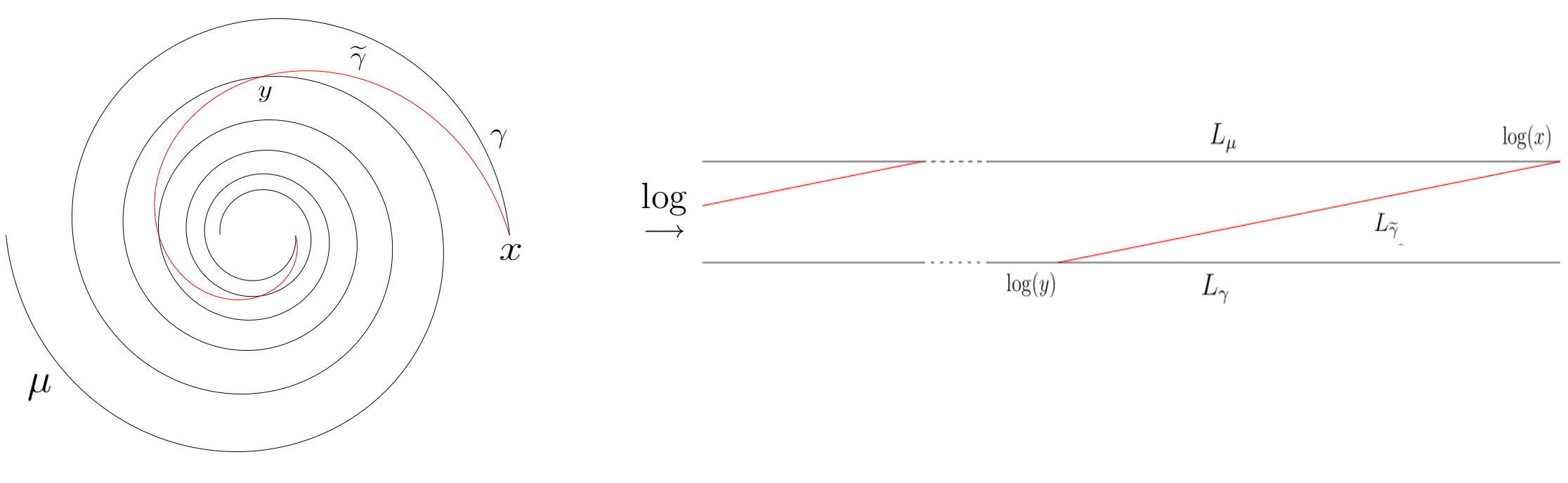
Figure 4: The $\vartheta$-trajectories are mapped by the logarithm to a horizontal strip, whereas the $\widetilde{\vartheta}$-trajectory is mapped to a straight line intersecting the strip at constant angles.

We consider the standard neighborhood $U$ around a weakly parabolic point, where $-qdz=\det(\Phi)=\frac{m}{z}dz$. In this neighborhood the $\vartheta$-trajectories are known to be logarithmic spirals (or straight lines) except for two exceptional values of $\vartheta_{c}$ where they become concentric circles around the parabolic point. We may parametrize all these spirals as $\mu(t)=\mu_{0}e^{i\varpi t}$ for differing values of $\mu_{0}$ and with $\varpi$ only depending on $\vartheta$ with $\operatorname{Re}(\varpi)<0$ as seen before. Let $\gamma$ and $\nu$ be the parts of two sides of the standard quadrilateral in this neighborhood. Their images together with $0$ separates the neighborhood into two regions, one of which corresponds to the inside of the quadrilateral, which shall be called $I$. As the $\vartheta$- trajectories don’t intersect, there are $\vartheta$-trajectories that lie in the complement $I^{c}$. We may take any one of them, say $\alpha$, to be a branch cut on $U$ and define a biholomorphic logarithm on $U\setminus\left(\operatorname{Im}(\alpha)\cup\left\{0\right\}\right)$. The domain of $\log$ then includes $I$. The logarithm now maps all the $\vartheta$-trajectories $\mu$ (excluding $\alpha$) to parallel lines $L_{\mu}$ which we rotate to be horizontal, so $L_{\gamma}$ and $L_{\nu}$ define a horizontal strip $S$. In the following $\log$ shall denote the composition of the logarithm and the rotation. In $\operatorname{Im}(\log)$ the left endpoints of the $L_{\mu}$ correspond to the values $\mu_{0}$ of $\mu$ at $t=0$ in $U$ while $0\in U$ is mapped to $-\infty$ to the left.

Now let $\widetilde{\gamma}$ be a $ca$-trajectory in for some $\widetilde{\vartheta}\neq\pm\vartheta$ that intersects $\gamma$ at some point $x$. The part of the curve starting at $x$ is then also mapped to a straight line at least until some point, where it intersects $\alpha$, which happens somewhere, as $\widetilde{\vartheta}\neq\pm\vartheta$ (cf. figure 4).

As the mapping is biholomorphic $L_{\widetilde{\gamma}}$ intersects $L_{\gamma}$ in the point $\log(x)$ at some non-zero angle $\beta$ which, as of Lemma 6.11 is constant for all intersection points. We recall that the $ca$-trajectories are oriented as running into $0$. For $\widetilde{\vartheta}$ close enough to $\vartheta$ we thus have that depending on wether $\widetilde{\vartheta}$ is bigger or smaller then $\vartheta$ the straight line $L_{\widetilde{\gamma}}$ continues in the strip $S$ or outside of $S$. We may thus take $\widetilde{\vartheta}$ arbitrarily close to $\vartheta$ and such that $L_{\widetilde{\gamma}}$ continues in the strip $S$. Being a straight line, $L_{\widetilde{\gamma}}$ will intersect $L_{\mu}$ at some point $\log(y)$ and the thus defined segment is the image of a part of the $ca$-trajectory $\widetilde{\gamma}$ inside $I$ under the logarithm. Thus $\widetilde{\gamma}$ intersects $\gamma$ and $\mu$ in $x=\gamma(t_{x})$ and $y=\mu(t_{y})$ stays inside $I$ for all $t_{x}<t<t_{y}$.

To calculate $t_{x}-t_{y}$ note that $L_{\gamma}=a_{1}+t\operatorname{Re}(\varpi)$ and $L_{\mu}=a_{2}+t\operatorname{Re}(\varpi)$ for $a_{1}\mathrel{\mathop{\mathchar 58\relax}}=\log(\gamma(0))$ and $a_{2}\mathrel{\mathop{\mathchar 58\relax}}=\log(\mu(0))$. Now $L_{\widetilde{\gamma}}$ has the form $L_{\widetilde{\gamma}}(t)=L_{0}+te^{i\beta}$ and intersects $L_{\gamma}$ in $t_{x}$ and $L_{\mu}$ in $t_{y}$. We obtain, that

$$\begin{split}a_{2}-a_{1}+\operatorname{Re}(\varpi)(t_{y}-t_{x})&=a_{2}+t_{y}\operatorname{Re}(\varpi)-(a_{1}+t_{x}\operatorname{Re}(\varpi))=L_{\mu}(t_{y})-L_{\gamma}(t_{x})\\ &=L_{\widetilde{\gamma}}(t_{y})-L_{\widetilde{\gamma}}(t_{x})=t_{y}e^{i\beta}-t_{x}e^{i\beta}=(t_{y}-t_{x})e^{i\beta}\\ \Rightarrow|t_{y}-t_{x}|&\leq\left|\frac{a_{2}-a_{1}}{e^{i\beta}-\operatorname{Re}(\varpi)}\right|=\mathrel{\mathop{\mathchar 58\relax}}d.\end{split}$$

Note that $a_{2}$ and $a_{1}$ are constants that only depend on the sides of the quadrilateral, as is $\varpi$. Also $\beta$ is constant for all intersections of $\widetilde{\gamma}$ and any part of any $\vartheta$-trajectory everywhere in $I$ as of Lemma 6.11 and the biholomorphicity of $\log$. Thus we conclude that $|t_{y}-t_{x}|=d$ is constant for all $\widetilde{\gamma}$-trajectories connecting $\gamma$ and $\mu$ in $U$. ∎

We have thus obtained the prerequisites for transporting the small flat section that was obtained along some side $\gamma$ of the quadrilateral $Q$ to another side $\mu$. For the proof we can now use ideas similar to the ones that helped befored.

Proposition 6.13

Let $\gamma$ and $\mu$ be two sides of the quadrilateral $Q$ sharing a vertex $p$ and $s$ the small flat section along $\gamma$. If $\zeta$ is small enough then $s$ evaluated along $\mu$ is of the form

$$s(t)=e^{-\Lambda_{2}(t)}\left(\begin{pmatrix}0\\ 1\end{pmatrix}+x^{r}\right),$$

with $x^{r}$ some $\mathbb{C}^{2}$-valued function with $|x^{r}|\leq\tilde{K}e^{-\delta R}$ for some constant $\tilde{K}$.

Proof.

To parallel transport the small flat section from one side of the quadrilateral to another we use the formulation via an integral equation as we have done before, only now we do not need to consider the integral up to infinity. We recall that in our set-up $\vartheta$ is fixed and we consider only those $\zeta$ which lie in the open half-plane $\mathbb{H}_{\vartheta}$. Thus $\zeta$ also lies in the half-plane $\mathbb{H}_{\widetilde{\vartheta}}$ for $\widetilde{\vartheta}$ close enough to $\vartheta$. Now we chose any point $p_{s}$ on $\mu$ close enough to the parabolic point, s. t. it lies in the neighborhood where the $ca$-trajectories may be expressed as logarithmic spirals. As of the previous Proposition 6.12 there exists a $\widetilde{\vartheta}$-trajectory $\alpha\mathrel{\mathop{\mathchar 58\relax}}[a,b]\to C$ with starting point $\alpha(a)=p_{s}$ and first intersection with $\gamma$ at $\alpha(b)=p_{e}$, s. t. the image of the curve is contained in the quadrilateral and $b-a\leq d$ for some constant $d$ that does not depend on the starting point $p_{s}$.

We now consider the solution of our ODE via variation of constants along $\alpha$, i. e. the parallel transport along $\alpha$ is the unique solution $x\mathrel{\mathop{\mathchar 58\relax}}[a,b]\to\mathbb{R}^{2}$ to the integral equation

$$x(t)=\begin{pmatrix}e^{\Lambda(t)-\Lambda(b)}&0\\ 0&1\end{pmatrix}x(b)-\int_{t}^{b}\begin{pmatrix}e^{\Lambda(t)-\Lambda(\tau)}&0\\ 0&1\end{pmatrix}\begin{pmatrix}e_{1}&e_{2}\\ e_{3}&-e_{1}\end{pmatrix}x(\tau)d\tau.$$ (14)

Note that $x(b)$ is now the ”initial value” of $x$ at the end point $p_{e}$ instead of the value at infinity. Here $\Lambda$ is again a primitive of $\lambda$ as above but now evaluated along $\alpha$. The theory developed before also holds for these usual Volterra equations where the integral does not go to infinity [Win10].

Thus we have a unique solution from which we would like to gather information about $x(a)=x(p_{s})$ on $\mu$ by estimating it against $x(b)=x(p_{e})$ on $\gamma$, using the techniques we already developed for the infinite case. As $\zeta$ lies in the half-plane $\mathbb{H}_{\widetilde{\vartheta}}$ we still have that $\Lambda(t)-\Lambda(\tau)$ has negative real part, which holds in particular for $\tau=b$. Thus the norm of the first matrix in the integrand is smaller then $1$ while the norm of the error matrix stays bounded by some $Ce^{-\delta R}$ as before for $\zeta$ small enough. As the domain of the integral is bounded by $d$ we obtain for large enough $R$ that the integral over the kernel is smaller then $1$, so a unique solution exists. As the matrix in the initial value function is also bounded by $1$, we obtain:

$$|x(t)|\leq\frac{\left|x(b)\right|}{1-dCe^{\delta R}}.$$

Plugging this estimate back into the the right hand side of the equation (14) we obtain for the integral

$$\begin{split}\left|\int_{t}^{b}\begin{pmatrix}e^{\Lambda(t)-\Lambda(\tau)}&0\\ 0&1\end{pmatrix}\begin{pmatrix}e_{1}&e_{2}\\ e_{3}&-e_{1}\end{pmatrix}x(\tau)d\tau\right|&\leq\int_{t}^{b}Ce^{-\delta R}\frac{\left|x(b)\right|}{1-dCe^{-\delta R}}d\tau\\ &\leq|x(b)|\widetilde{C}e^{-\delta R}\end{split}$$ (15)

for some uniform constant $\widetilde{C}$. The full equation (14) thus shows us, that we have:

$$x(t)=\begin{pmatrix}e^{\Lambda(t)-\Lambda(b)}&0\\ 0&1\end{pmatrix}x(b)+v(t)$$ (16)

where $|v(t)|\leq|x(b)|\widetilde{C}e^{-\delta R}$ along the whole segment. As $\Lambda(t)-\Lambda(\tau)\leq 0$ along the segment, we obtain the estimate

$$|x(t)|\leq|x(b)|(1+Ce^{-\delta R}).$$ (17)

In particular we have the (in)equalities 16 and 17 for $t=a$, i. e. for large enough $R$ the endpoints $x(a)$ and $x(b)$ on the two sides of the quadrilateral differ by some (bounded) multiplicative factor in the first component (that vanishes for $\zeta\to 0$ or $R\to\infty$) and an added vector which is bounded by the norm of the function on the other side multiplied with some exponentially suppressed constant. Note that this argument is valid for all $\widetilde{\vartheta}$ segments arbitrarily close to the weakly parabolic point $p$ and the upper bounds can be chosen to be valid for all arbitrarily close segments. Now $x(b)$ is the value of the section on the side where the small flat section was defined which is bounded near $p$, so the value on the other side is also bounded. This already shows that the transported section along the second side must also be a small flat section as the big sections would have to surpass every upper bound somewhere close to the parabolic point. Thus we know that the section has a limit along the second side going into the parabolic point and the first component of this limit must vanish. As $x(b)$ has limit $(0,1)^{t}$ going into $p$ along $\gamma$ the limit along the second side $\mu$ is $(0,1+\epsilon)$ for some constant $\epsilon$ with norm $|\epsilon|\leq Ce^{-\delta R}$ for some uniform constant $C$ for $\zeta$ small enough.

Therefore the section along $\mu$ is the solution of

$$\begin{split}x(t)=\begin{pmatrix}0\\ 1+\epsilon\end{pmatrix}-\int_{t}^{\infty}\begin{pmatrix}e^{\Lambda(t)-\Lambda(\tau)}&0\\ 0&1\end{pmatrix}\begin{pmatrix}e_{1}(\tau)&e_{2}(\tau)\\ e_{3}(\tau)&-e_{1}(\tau)\end{pmatrix}x(\tau)d\tau,\end{split}$$

where $\Lambda$ and the integral are now taken along $\mu$. As $\epsilon$ is exponentially bounded it follows with the same arguments as in Proposition 6.7 that $x$ is of the form

$$x(t)=\begin{pmatrix}0\\ 1\end{pmatrix}+x^{r},$$

with $x^{r}$ some $\mathbb{C}^{2}$-valued function with $|x^{r}|\leq\tilde{K}e^{-\delta R}$ for some constant $\tilde{K}$. Again the form for $s$ follows readily. ∎

We can now proceed to build the $\mathcal{X}_{E}$ coordinate (where we mostly suppress the explicit dependence on the triangulation, $q$ and $\vartheta$ in the notation). For this consider again the standard quadrilateral $Q$ associated to an edge $E$ of the triangulation with vertices given by four weakly parabolic points $p_{i}$. We want to build the $\wedge$-product according to the definition 3.17 of $\mathcal{X}_{E}$. But to do so we have to consider that our calculations up until now was always validated on contractible subsets of the standard annulus $S$ in $Q$ and we already introduced different primitives for $\lambda$ in the different patches belonging to two different $\vartheta$-curves. This now has to be done for all of the four sections of the quadrilateral. Additionally for each vertex $p_{i}$ there are two sides joining $p_{i}$ and thus two small flat sections of $\nabla(\zeta)$ which are given by the solution of the integral equation along these two curves, from which one has to be chosen. Our way for doing this is the following:

First we remember that we fixed the orientation for the $\vartheta$-curves depending on $q^{1/2}$ (cf. the discussion of the flatness equation (11)). This implies that if one side of the quadrilateral $Q$ is given by a curve oriented as running into a vertex $p_{i}$ (for $t\to\infty$) the other side of $Q$ sharing the vertex $p_{i}$ is also oriented as running into $p_{i}$. Thus two vertices of $Q$ are points into which the $\vartheta$-curves run, and the other two vertices are points from which the curves emerge. We start with labeling one of the points into which the curves run as $p_{1}$ and label the following vertices clockwise. Now we label the side joining $p_{4}$ and $p_{1}$ as $\gamma_{1}$ with is thus oriented in such a way that $\gamma_{1}$ converges to $p_{1}$ for $t\to\infty$. The other side joining $p_{1}$ connects $p_{1}$ and $p_{2}$ and shall be labeled as $\gamma_{2}$ and is also oriented in such a way that $\gamma_{2}$ converges to $p_{1}$ for $t\to\infty$. Now $p_{2}$ will be a vertex from which $\vartheta$-curves emerge, while $p_{3}$ will be of the same type as $p_{1}$. So we proceed for $\gamma_{3}$ and $\gamma_{4}$ in the same way as for $\gamma_{1}$ and $\gamma_{2}$, just now for the vertex $p_{3}$. In this way we obtain four oriented curves as sides of $Q$. For each of the vertices $p_{i}$ let $\Lambda^{i}_{1}$ be a primitive of $\lambda_{1}\mathrel{\mathop{\mathchar 58\relax}}=-\frac{R}{\zeta}q^{1/2}-R\zeta q^{1/2}-\overline{a_{1}}d\overline{z}+a_{1}dz$ and $\Lambda^{i}_{2}$ a primitive of $\lambda_{2}\mathrel{\mathop{\mathchar 58\relax}}=-\frac{R}{\zeta}q^{1/2}-R\zeta q^{1/2}+\overline{a_{2}}d\overline{z}-a_{2}dz$ defined on a simply connected neighborhood $U_{i}$ of $\gamma_{i}$ and $\gamma_{i+1}$ in $S$. Note that these primitives exist as $p$ is holomorphic and the frame was chosen in such a way that $d(\overline{a_{j}}-a_{j})=0$. Evaluated along a $\vartheta$-curve these primitives become the primitives that were used in the calculations above (cf. equation (11)). Finally for each vertex we choose $s^{i}$ to be the small flat section along $\gamma_{i}$ defined using the primitives $\Lambda_{j}^{i}$ and extended to sections of $\nabla(\zeta)$ on $U_{i}$ (cf. figure 5). This extension is possible as the $U_{i}$ are simply connected and $\nabla(\zeta)$ is flat. We note that this way of choosing the sections is not necessary. Other choices lead to the same $\mathcal{X}$ coordinates as the small flat sections only differ by a (constant) complex scalar, which cancels in the final $\wedge$-product. This also justifies the arbitrary choice of the ”initial value at infinity” as $(0,1)^{t}$. Thus we may now define the $\mathcal{X}$- coordinate.

Figure 5: A standard quadrilateral given by four oriented $\vartheta$-curves $\gamma_{i}$. The orange crosses denote the zeroes of $-q$ and the blue circles the weakly parabolic points. The blue crosses denote the evaluation points for the small flat sections and the blue lines are curves along which two of the $\wedge$-products are transported. The red outer and inner ”circles” are the boundary of a standard annulus. Together with the red straight arc they form the boundary of the simply connected neighborhood $U_{1}$ for $\gamma_{1}$.

Proposition 6.14

Let $Q$ be a standard quadrilateral with vertices $p_{i}$ and small flat sections chosen as described above. Then for $z_{1}\in U_{1}\cap U_{4}$ and $z_{3}\in U_{2}\cap U_{3}$ the product

$$-\frac{\left(s^{1}\wedge s^{2}\right)(z_{1})}{\left(s^{4}\wedge s^{1}\right)(z_{1})}\frac{\left(s^{3}\wedge s^{4}\right)(z_{3})}{\left(s^{2}\wedge s^{3}\right)(z_{3})}=\mathrel{\mathop{\mathchar 58\relax}}-\frac{\left(s^{1}\wedge s^{2}\right)\left(s^{3}\wedge s^{4}\right)}{\left(s^{4}\wedge s^{1}\right)\left(s^{2}\wedge s^{3}\right)}=\mathrel{\mathop{\mathchar 58\relax}}\mathcal{X}_{E}$$

is well defined, non-zero and independent of the evaluation points $z_{1}$, $z_{3}$.

Proof.

By construction the $\wedge$-products are defined on $z_{1}$ and $z_{3}$. As of Propositions 6.8 and 6.13 it follows that all of the $\wedge$-products are non-zero, so $\mathcal{X}$ is well defined and non-zero. The independence of the evaluation points is also true by construction, cf. the discussion preceding the definition 3.17. ∎

So $\mathcal{X}_{E}$ only depends on the parameters of the Higgs pair, $\zeta$, $\vartheta$ and the choice of quadrilateral. Thus if we fix $\zeta$ and $\vartheta$ we obtain functions on $\mathcal{M}$. As described in section 3.2 it follows from the work of Fock and Goncharov [FG06] and the treatment in [GMN13a] that the collection of these functions for all edges are actually coordinates of $\mathcal{M}$, called the canonical coordinates.

Now consider the cycle $\gamma_{E}\in H_{1}(\Sigma^{\prime}_{q};\mathbb{Z})$ encircling the preimage of the two zeroes inside of $Q$ in the (punctured) spectral curve $\Sigma^{\prime}_{q}$. One of the key claims in [GMN13a] is that in the $\zeta\rightarrow 0$ asymptotic the period integral $\oint_{\gamma}\left(q^{1/2}\right)^{\ast}$ emerges as the leading term for the $\mathcal{X}$-coordinates, where $\left(q^{1/2}\right)^{\ast}$ denotes the Liouville (tautological) $1$-form on $T^{\ast}C$ That is by pushing $\gamma_{E}$ down to a cycle on $C$ (which we’ll also denote by $\gamma_{E}$) one has $\mathcal{X}_{\gamma_{E}}\sim c_{\gamma_{E}}\exp(\frac{R}{\zeta}\oint_{\gamma_{E}}q^{1/2}dz)$ for some constant $c_{\gamma_{E}}$. Their conjecture was based on the WKB method but had not been rigorously proven until now. With the calculations done above we can now achieve this, but one technical detail has to be accounted for. As noted above [GMN13a] used the convention that the matrix representing $\nabla(\zeta)$ is traceless, which leads to a $z$-invariance of the $\wedge$-products even before taking the quotient in the $\mathcal{X}$-definition. Thus they can evaluate the sections on each curve so that the primitives combine in just the right way to create the period integral. In our set-up the the connection matrix is not traceless, so this independence does not hold. Additionally from Propositions 6.8 and 6.13 we only have the detailed description of $s^{i}\wedge s^{k}$ along the curve connecting the vertices $p_{i}$ and $p_{k}$. But the definition of $\mathcal{X}$ implies that at least two of the $\wedge$-products have to be evaluated in a point on some other side. We have to account for this by parallel transporting two of the $\wedge$-products to other sides. As the $s^{i}\wedge s^{k}$ are sections of a line bundle this is done rather easily.

Lemma 6.15

Let $\gamma_{i}$ and $\gamma_{i+1}$ be the sides of a standard quadrilateral $Q$ sharing the vertex $p_{i}$, with $z_{i}\in\text{Im}(\gamma_{i})$ and $z_{i+1}\in\text{Im}(\gamma_{i+1})$ two points on these sides of $Q$. Let $s^{i}$ and $s^{i+1}$ be the corresponding small flat sections defined on the neighborhoods $U_{i}$ and $U_{i+1}$.

Then for every curve $\mu\in U_{i}\cap U_{i+1}$ connecting $z_{i}$ and $z_{i+1}$ it holds:

$$s^{i}\wedge s^{i+1}(w_{2})=e^{\int_{\mu}(a_{1}+a_{2})dz-\overline{a_{1}+a_{2}}d\overline{z}}s^{i}\wedge s^{i+1}(w_{1}),$$

Proof.

From Proposition 6.13 and Corollary 6.9 $s^{i}$ and $s^{j}$ define a fundamental system for the linear ODE $s^{\prime}(t)=B(t)s(t)$ given by the flatness equation (11) along $\mu$. The equation is now simply an application of Liouville’s formula where we note that the only part of the connection matrix of $\nabla(\zeta)$ that is not traceless comes from the leading part of the Chern connection (cf. Remark 4.12), which is just $(a_{1}+a_{2})dz-\overline{a_{1}+a_{2}}d\overline{z}$ (cf. equation (12)). ∎

Finally we can see the emergence of the period integrals.

Theorem 6.16

Let $Q$ be the standard quadrilateral for an edge $E$ of a $\vartheta$-triangulation of $C$. The canonical coordinate for $Q$ can be expressed as

$$\mathcal{X}_{E}=-(1+r_{q})\exp\left(\frac{R}{\zeta}\oint_{\gamma_{E}}q^{1/2}+R\zeta\oint_{\gamma_{E}}\overline{q^{1/2}}+\oint_{\gamma_{E}}\overline{a_{1}}d\overline{z}-a_{1}dz\right),$$

where $r_{q}$ is exponentially suppressed in $R$ for small enough $\zeta$, and $\gamma_{E}$ is the projection of a cycle in $H_{1}(\Sigma^{\prime}_{q};\mathbb{Z})$ corresponding to the edge $E$, that is a simple closed curve in $Q$ encircling the two zeros of $q$ once.

Proof.

With the same notations as before we choose a point $z_{i}\in\text{Im}(\gamma_{i})$ on each of the sides of the standard quadrilateral $Q$ and curves $\mu_{kl}$ connecting the points $z_{k}$ and $z_{l}$ in $U_{k}\cap U_{l}$ (cf. figure 5). For abbreviation we write $\text{tr}\left(\nabla(\zeta)\right)\mathrel{\mathop{\mathchar 58\relax}}=\overline{a_{1}+a_{2}}d\overline{z}-(a_{1}+a_{2})dz$. Then using Lemma 6.15 to parallel transport the $\wedge$-products to the sides where they can be evaluated as in corollary 6.10 we obtain the following expression:

$$\begin{split}\mathcal{X}_{E}&=-\frac{\left(s^{1}\wedge s^{2}\right)(z_{2})\left(s^{3}\wedge s^{4}\right)(z_{4})}{\left(s^{4}\wedge s^{1}\right)(z_{2})\left(s^{2}\wedge s^{3}\right)(z_{4})}=-\frac{\left(s^{1}\wedge s^{2}\right)(z_{2})\left(s^{3}\wedge s^{4}\right)(z_{4})}{\left(s^{4}\wedge s^{1}\right)(z_{1})\left(s^{2}\wedge s^{3}\right)(z_{3})}e^{-\int_{\mu_{2}}\text{tr}\left(\nabla(\zeta)\right)-\int_{\mu_{4}}\text{tr}\left(\nabla(\zeta)\right)}\\ &=-\frac{e^{-\Lambda^{1}_{2}(z_{2})+\Lambda^{2}_{1}(z_{2})}(1+r_{12})e^{-\Lambda^{3}_{2}(z_{4})+\Lambda^{4}_{1}(z_{4})}(1+r_{34})}{e^{\Lambda^{4}_{1}(z_{1})-\Lambda^{1}_{2}(z_{1})}(1+r_{41})e^{\Lambda^{2}_{1}(z_{3})-\Lambda^{3}_{2}(z_{3})}(1+r_{23})}e^{-\int_{\mu_{2}}\text{tr}\left(\nabla(\zeta)\right)-\int_{\mu_{4}}\text{tr}\left(\nabla(\zeta)\right)}\\ &=-(1+r_{q})\cdot e^{\Lambda^{1}_{2}(z_{1})-\Lambda^{1}_{2}(z_{2})+\Lambda^{2}_{1}(z_{2})-\Lambda^{2}_{1}(z_{3})+\Lambda^{3}_{2}(z_{3})-\Lambda^{3}_{2}(z_{4})+\Lambda^{4}_{1}(z_{4})-\Lambda^{4}_{1}(z_{1})}e^{-\int_{\mu_{2}}\text{tr}\left(\nabla(\zeta)\right)-\int_{\mu_{4}}\text{tr}\left(\nabla(\zeta)\right)},\end{split}$$

where the $r_{kl}$ denote the corresponding remainder terms and $r_{q}$ is the term emerging from all of the $r_{kl}$, which is thus, as of Corollary 6.10, exponentially suppressed in $R$.

The key step is now noticing that $\Lambda^{i}_{j}(z_{k})-\Lambda^{i}_{j}(z_{l})=\int_{\mu_{lk}}\lambda_{j}$ leads to the desired period integrals, which is a bit concealed here as we work with the different $\lambda_{j}$, emerging from tr$\nabla(\zeta)\neq 0$. So at first we obtain the following:

$$\mathcal{X}_{E}=-(1+r_{q})\exp\left(\int_{\mu_{21}}\lambda_{2}+\int_{\mu_{32}}\lambda_{1}+\int_{\mu_{43}}\lambda_{2}+\int_{\mu_{14}}\lambda_{1}\right)\exp\left(-\int_{\mu_{12}}\text{tr}\left(\nabla(\zeta)\right)-\int_{\mu_{34}}\text{tr}\left(\nabla(\zeta)\right)\right).$$

To put these integrals together we note that $\lambda_{1}$ and $\lambda_{2}$ differ only by containing expressions of $a_{1}$ or $a_{2}$. So for the parts involving $q^{1/2}$ we already obtain a period integral along a simple closed curve $\mu$ encircling the two zeroes of $q$, while we observe the following cancellation for the rest

$$\begin{split}\mathcal{X}_{E}&=-(1+r_{q})\exp\left(-\frac{R}{\zeta}\oint_{\mu}q^{1/2}-R\zeta\oint_{\mu}\overline{q^{1/2}}\right)\\ &\exp\left(\int_{\mu_{21}}\overline{a_{2}}d\overline{z}-a_{2}dz-\int_{\mu_{32}}\overline{a_{1}}d\overline{z}-a_{1}dz+\int_{\mu_{43}}\overline{a_{2}}d\overline{z}-a_{2}dz-\int_{\mu_{14}}\overline{a_{1}}d\overline{z}-a_{1}dz\right)\\ &\exp\left(\int_{\mu_{12}}\overline{a_{1}}d\overline{z}+\overline{a_{2}}d\overline{z}-\int_{\mu_{12}}a_{1}dz+a_{2}dz+\int_{\mu_{34}}\overline{a_{1}}d\overline{z}-\overline{a_{2}}d\overline{z}-\int_{\mu_{34}}a_{1}dz+a_{2}dz\right)\\ &=-(1+r_{q})\exp\left(-\frac{R}{\zeta}\oint_{\mu}q^{1/2}-R\zeta\oint_{\mu}\overline{q^{1/2}}+\oint_{\mu}a_{1}dz-\overline{a_{1}}d\overline{z}\right).\end{split}$$ (18)

As $q^{1/2}$ is holomorphic on $\mathcal{C}$, the integral does not depend on the specific curve but only on its homotopy class. For the term $a\mathrel{\mathop{\mathchar 58\relax}}=\overline{a_{1}}d\overline{z}-a_{1}dz$ we note that this corresponds to the entries of the Chern connection $A_{0}$ of $\overline{\partial}_{E}$ w. r. t. the limiting metric $h_{0}$, and this solves the decoupled Hitchin equations 4.1. Thus $A_{0}$ is a flat connection and this implies $da=0$, so this integral is also defined on the corresponding homotopy class and we obtain the period integrals on $\mathcal{C}$. The construction as outlined in section 3.3 and described in more detail in [GMN13a] guarantees that the signs match in the right way when comparing $\mu$ with $\gamma_{E}$ coming from a cycle in $H_{1}(\Sigma^{\prime}_{q};\mathbb{Z})$, leading to the desired result. ∎

As noted before the $\oint_{\gamma_{E}}q^{1/2}$ should be thought of as living on the spectral cover, where the tautological $1$-form is integrated along $\gamma_{E}\in H_{1}(\Sigma^{\prime}_{q};\mathbb{Z})$. As [GMN13a] already noted the period integrals would vanish if $p^{1/2}$ could be well defined on the whole quadrilateral. But as we had to cut out a disc around the zeroes of $p$, i. e. the branch points of the spectral curve, we obtain some nonzero value. Following the notation of GMN the periods are denoted $Z_{\gamma}\mathrel{\mathop{\mathchar 58\relax}}=\tfrac{1}{\pi}\oint_{\gamma}q^{1/2}$. They give ”special coordinates” on the Hitchin Base $\mathcal{B}^{\prime}$ corresponding to its special Kähler metric. Similarly note that $\oint_{\gamma}a_{1}dz-\overline{a_{1}}d\overline{z}$ is imaginary-valued and one can show that the functions $\theta$ with $i\theta\mathrel{\mathop{\mathchar 58\relax}}=\oint_{\gamma}\overline{a_{1}}d\overline{z}-a_{1}dz$ for $\gamma_{E}\in H_{1}(\Sigma^{\prime}_{q};\mathbb{Z})$ give coordinates of the torus fibers of the Hitchin fibration, thus completing the set of coordinates for the semiflat metric in $\mathcal{M}^{\prime}$.

One might wonder at this point that the coordinates don’t depend on $a_{2}$ anymore which was one of the two entries of the holomorphic structure from which the Chern connection of the Higgs pair was constructed. The vanishing of this term does not lead to a loss of information as the connections for two Higgs pairs only differ by a traceless matrix so all necessary information is encoded in one of the diagonal entries.

Let us now proceed to show a property of $\mathcal{X}_{E}$, which will be important for the twistorial construction later on. First we want to expand the definition of $\mathcal{X}_{E}$ to large $\zeta$, for which we first have to check whether the small flat sections can be treated in the same way as before for large $\zeta$. We do this by considering $\nabla\left(-1/\overline{\zeta}\right)$ for small $\zeta$. It is useful in this context to switch the frame and consider the flatness equation $0=\nabla(\zeta)s$ in an $h$-unitary frame. So in the following the indices $h$ and $h_{0}$ denote the local expression in the $h$-unitary and $h_{0}$-unitary frame (where the second one is the frame $F$ we used up until now).

In this new frame $H_{h}=E_{2}$ locally and so $\varphi_{h}^{\ast_{h}}=\overline{\varphi_{h}}^{t}$ and $A_{h_{\overline{z}}}^{\ast_{h}}=\overline{A_{h_{\overline{z}}}}^{t}$. By construction the change of basis matrix from the $h$-unitary frame to the $h_{0}$-unitary frame is $g^{-1}$. So if $s_{h_{0}}$ is the local expression of a solution of the flatness equation in the $h_{0}$-unitary frame, $s_{h}\mathrel{\mathop{\mathchar 58\relax}}=gs_{h_{0}}$ is the local expression in the $h$-unitary frame. Now from

$$g\circ\left(\nabla_{h_{0}}\right)\circ g^{-1}s_{h}=g\circ\left(\nabla_{h_{0}}s_{h_{0}}\right)=0$$

it follows, that $s_{h}$ is a solution of the flatness equation in the $h$-unitary frame.

We take the $\zeta$-dependence of $B_{h}$ into account and calculate $\overline{B_{h}}^{t}$ using the fact that $A$ is $h$-unitary:

$$\begin{split}\overline{B_{h}}^{t}(\zeta,t)&=\left(-\frac{R}{\overline{\zeta}}\overline{\varphi}^{t}-\overline{A_{h_{z}}}^{t}\right)\overline{z}^{\prime}+\left((-R\overline{\zeta})\overline{\varphi^{\ast_{h}}}^{t}-\overline{A_{h_{\overline{z}}}}^{t}\right)z^{\prime}\\ &=\left(-\frac{R}{\overline{\zeta}}\varphi^{\ast_{h}}+A_{h_{\overline{z}}}\right)\overline{z}^{\prime}+\left((-R\overline{\zeta})\varphi+A_{h_{z}}\right)z^{\prime}\\ &=-B_{u}(-\tfrac{1}{\overline{\zeta}},t).\end{split}$$

Let $s$ and $b$ denote the small flat sections for two parabolic points $p_{1}$ and $p_{2}$ joined by $\gamma$. From the Proposition 6.8 we know that they are linearly independent and thus form a fundamental system $X$ for the ODE given by $B_{h}(\zeta)$:

$$X=\begin{pmatrix}s^{1}_{h}&b^{1}_{h}\\ s^{2}_{h}&b^{2}_{h}\end{pmatrix}.$$

Combining the result above with a standard argument we obtain

$$\begin{split}0&=\frac{d(XX^{-1})}{dt}=X^{\prime}X^{-1}-X\left(X^{-1}\right)^{\prime}=B_{h}(\zeta)XX^{-1}-X\left(X^{-1}\right)^{\prime}\\ &\Rightarrow\left(X^{-1}\right)^{\prime}=-X^{-1}B_{h}(\zeta)\\ &\Rightarrow\left(\overline{X^{-1}}^{t}\right)^{\prime}=-\overline{B_{h}(\zeta)}^{t}\overline{X^{-1}}^{t}\\ &\Rightarrow\left(\overline{X^{-1}}^{t}\right)^{\prime}=B_{h}(-\frac{1}{\overline{\zeta}})\overline{X^{-1}}^{t}.\end{split}$$

So we see that a fundamental system for $-\frac{1}{\overline{\zeta}}$ is given by

$$\overline{X^{-1}}^{t}=\frac{1}{s^{1}_{h}b^{2}_{h}-s^{2}_{h}b^{1}_{h}}\begin{pmatrix}\overline{b^{2}_{h}}&-\overline{s^{2}_{h}}\\ -\overline{b^{1}_{h}}&\overline{s^{1}_{h}}\end{pmatrix}.$$

Thus we see that the sections given by these rows of this matrix are flat sections for $-\tfrac{1}{\overline{\zeta}}$. We denote them by $\tilde{s}\mathrel{\mathop{\mathchar 58\relax}}=\frac{1}{s^{1}_{h}b^{2}_{h}-s^{2}_{h}b^{1}_{h}}(-\overline{s^{2}_{h}},\overline{s^{1}_{h}})$ and $\tilde{b}\mathrel{\mathop{\mathchar 58\relax}}=\frac{1}{s^{1}_{h}b^{2}_{h}-s^{2}_{h}b^{1}_{h}}(\overline{b^{2}_{h}},-\overline{b^{1}_{h}})$. We would like these sections to be the corresponding small flat sections, so we have to check how they behave as $t\to\infty$. But to be able to compare them to the sections considered before we first have to transform back to the $h_{0}$-unitary frame. Using the fact that the transform is given by $g^{-1}$ and using Lemma 4.9 a short calculation shows that $\tilde{s}$ decays exponentially for $\to\infty$, while $\tilde{b}$ grows. Thus we have the same structure as before and can expand our choice of small flat sections to $-\tfrac{1}{\overline{\zeta}}$ for small $\zeta$. As before there is a complex $1$-dimensional subspace of small flat sections and we may chose a unique one by demanding the a certain limit for $t\to\infty$ after extracting the leading term. Again this choice is of no real importance as complex factors cancel in the final expression for $\mathcal{X}_{E}$.

Now we have to remember that $s$ and $b$ are the small flat section for the vertices $p_{1}$ and $p_{2}$ for some small $\zeta$ and a $\vartheta$-curve running from the $p_{2}$ into $p_{1}$. We want $\tilde{s}$ to be the small flat section for some vertex. As explained above the behaviour is just right but we have to take care of the correct domain in the $\zeta$-plane. By construction the decoration at any parabolic point is only defined if $\zeta\in\mathbb{H}_{\vartheta}$. Now $-\frac{1}{\overline{\zeta}}$ is not in $\mathbb{H}_{\vartheta}$ as it has exactly the opposite phase. But it is thus in the half space $\mathbb{H}_{\vartheta+\pi}$. Now it remains to be checked whether $\tilde{s}$ is small along a $ca$-trajectory with angle $\vartheta+\pi$. At first $ca$-trajectories are only defined up to orientation, i. e. $\gamma$ is also a $ca$-trajectory for $\vartheta+\pi$ as $e^{i(\vartheta+\pi)}=-e^{i\vartheta}$. But now the orientation is the opposite one if we demand $q^{1/2}(\gamma^{\prime})=-e^{i\vartheta}$ as before. Thus $\tilde{s}$ is now the small flat section for $p_{2}$ and $\tilde{b}$ for $p_{1}$, which corresponds to a change of the decoration at both vertices, which is called pop in [GMN13a]. In the full picture for a standard quadrilateral this amounts to switching all of the decorations, which is called an omnipop. For our calculations we note that the omnipop leads to switching all sections in the wedge products of $\mathcal{X}_{E}$, leading to four changes of the sign, which thus overall cancel. We note that GMN use the equality under the omnipop as a quite powerful tool to determine the BPS spectrum, but here it will only be used now to obtain the so called reality condition.

Theorem 6.17

For small enough $\zeta$ the $\mathcal{X}$ coordinates obey the reality condition

$$\mathcal{X}_{\gamma}^{\vartheta}(\zeta)=\overline{\mathcal{X}_{\gamma}^{\vartheta+\pi}(-1/\overline{\zeta})}.$$

Proof.

With the considerations from above and the notation as for Theorem 6.16 we obtain the following equality:

$$\begin{split}&\mathcal{X}_{E}^{T(\vartheta+\pi)}(-1/\overline{\zeta})\\ &=\frac{\begin{pmatrix}-\overline{s^{1}_{2}}\\ \overline{s^{1}_{1}}\end{pmatrix}\wedge\begin{pmatrix}-\overline{s^{2}_{2}}\\ \overline{s^{2}_{1}}\end{pmatrix}}{\overline{s^{1}\wedge s^{2}}^{2}}(z_{2})\frac{\begin{pmatrix}-\overline{s^{3}_{2}}\\ \overline{s^{3}_{1}}\end{pmatrix}\wedge\begin{pmatrix}-\overline{s^{4}_{2}}\\ \overline{s^{4}_{1}}\end{pmatrix}}{\overline{s^{3}\wedge s^{4}}^{2}}(z_{4})\left(\frac{\begin{pmatrix}-\overline{s^{4}_{2}}\\ \overline{s^{4}_{1}}\end{pmatrix}\wedge\begin{pmatrix}-\overline{s^{1}_{2}}\\ \overline{s^{1}_{1}}\end{pmatrix}}{\overline{s^{1}\wedge s^{2}}\overline{s^{3}\wedge s^{4}}}(z_{2})\frac{\begin{pmatrix}-\overline{s^{2}_{2}}\\ \overline{s^{2}_{1}}\end{pmatrix}\wedge\begin{pmatrix}-\overline{s^{3}_{2}}\\ \overline{s^{3}_{1}}\end{pmatrix}}{\overline{s^{1}\wedge s^{2}}\overline{s^{3}\wedge s^{4}}}(z_{4})\right)^{-1}\\ &=\frac{\overline{s^{1}\wedge s^{2}}(z_{4})\overline{s^{3}\wedge s^{4}}(z_{2})}{\overline{s^{4}\wedge s^{1}}(z_{2})\overline{s^{2}\wedge s^{3}}(z_{4})}.\end{split}$$

Now we can again use Liouville’s formula to transport $s^{1}\wedge s^{2}$ from $z_{4}$ to $z_{2}$ and $s^{3}\wedge s^{4}$ from $z_{2}$ to $z_{4}$. The emerging exponential factors then cancel an we obtain $\mathcal{X}_{E}^{T(\vartheta+\pi)}(-1/\overline{\zeta})=\overline{\mathcal{X}^{T(\vartheta)}(\zeta)}$. By construction

$$\gamma_{E}^{\vartheta}=-\gamma_{E}^{\vartheta+\pi},$$

and thus combined we obtain

$$\mathcal{X}_{\gamma}^{(\vartheta)}(\zeta)=\overline{\mathcal{X}_{\gamma}^{\vartheta+\pi}(-1/\overline{\zeta})}.$$

∎

Remark 6.18

Before concluding this section we may shortly consider the case of degenerate edges. As stated in remark 3.15 we do not work this out in detail here as we can mostly adapt the way this is done in [GMN13a]. The basic idea is that in the case of a degenerate edge $E$ corresponding to a degenerate triangle the corresponding quadrilateral also degenerates and one has to consider a covering surface on which the necessary cycles can be defined. After appropriately matching the definitions one obtains cycles consisting of two loops running in opposite directions around the two lifts of a vertex on the spectral cover. The period integrals are then given by the residues at the vertex which are fixed for the moduli space.

But GMN also show that in this case $\mathcal{X}_{E}=\mu^{2}$ where $\mu$ is the clockwise monodromy around the degenerate vertex, which they have calculated from their Frobenius analysis (cf. the discussion following equation (10)). This is the only part in which we differ, as we have not obtained the small flat section in this way. But our way works just as good, as we may also evaluate our small flat sections along a circle around the degenerate vertex. Indeed, there is always some $\vartheta$ such that the $\vartheta$-curves are circles around the poles of $q$. We can thus simply use our analysis just like before and obtain the monodromy data, which matches the one from GMN. One then sees directly by comparing with the residue data that $\mathcal{X}$ again becomes dominated by the period integral without any further calculations.

6.3 Concerning the derivatives of the coordinates

In the last section of this part we want to check the logarithmic derivative of the $\wedge$-product as the hyperkähler metric will be build out of this. After considering the possibility of differentiating at all the important result here will be, that the logarithmic derivative has only simple poles for $\zeta\to 0$ or $\zeta\to\infty$. To show this we first take a look at the derivative $\partial_{\epsilon}$ of $x\wedge y$, where we differentiate with respect to some coordinate of the moduli space which is a parameter $\epsilon$ of the ODE. Generally, if the sections are differentiable we have the usual product rule

$$\partial_{\epsilon}(x\wedge y)=(\partial_{\epsilon}x)\wedge y+x\wedge(\partial_{\epsilon}y).$$

Note that we do not need to consider the variation of the frame as this can be taken to be locally constant in $\epsilon$ and taking if necessary a global change of basis which cancels in the definition of $\mathcal{X}$. Thus we need to differentiate the solutions of the integral equation, but before we can do carry out the explicit calculations there is one rather technical point we have to address.

Remark 6.19

In this chapter we will assume that the coefficients of the local expressions of our objects, like the Higgs field, depend differentiably on differentiable coordinates of the moduli space. As long as we only considered the functions $\mathcal{X}$ at some point on the moduli space this was not important, but as we begin to describe the derivatives we are moving in the moduli space and one has to lift families of elements of the moduli spaces (i. e. the equivalence classes) to corresponding families of representatives in such a way, that the differentiable structure is preserved. The possibility of such a differentiable choice of representatives is basically built directly into the construction of the moduli space as a Hyperkähler quotient, which is why we won’t go into the technical details here. Instead we refer to the thorough explanation of the process of building the quotient in [May16].

But this choice of representatives only addresses the part of the story where the objects as global functions dependd differentiable on the coordinates. As we are going to work with the local expressions, we also have to consider how the differentiability survives, the process of evaluation in a local frame. As long as the frame is fixed for a curve of Higgs fields $\phi_{t}$ one obtains the differentiable dependence of the matrix coefficients as the evaluation at a point in a local frame defines a bounded linear operator. But in our construction in section 4.1 we adapted the frame to the Higgs field by taking a frame consisting of eigenvectors of $\phi$. The $\mathcal{X}$-coordinates themselves are independent of any frame, but we have to make sure that our construction of the small flat sections from the corresponding integral equations works. Therefore it needs to be possible to chose the eigenvectors of $\phi_{t}$ in such a way that they vary differentiably with the entries of the local expressions of $\phi_{t}$ in the fixed frame. But this follows from a short calculation in linear algebra, so everything works out and we have the desired structure of a diagonal leading term plus some small error matrix. However, at this point we have only diagonalized the Higgs field $\phi_{t}$ and not scaled the frame to a standard form, as was also done in section 4.1. This should also be possible as all the transformations are differentiable, but we actually don’t have to adapt the frames in this way. Indeed, by not adapting the frame to the limiting metric and holomorphic structure, we only obtain a slightly different expression of the leading term in the flatness equation and some additional finite multiplicative factors in the entries of the error matrix. As they are finite, they don’t change the analytical properties of our integral equation at all. Therefore we can safely ignore these changes and continue to work with the form of our equation we used up until now.

Lemma 6.20

The small flat sections are differentiable with respect to any differentiable coordinate $\epsilon$ of $\mathcal{M}_{R}$ and the derivative of the remainder-term is bounded by some uniform constant for small enough $\zeta$.

Proof.

The leading term $e^{-\Lambda_{2}}$ is differentiable by construction. So what we have to consider is the remainder term. We want to use Theorem 5.11, so we have to check that the kernel is of product type of second order w. r. t. a coordinate $\epsilon$ of the moduli space $\mathcal{M}_{R}$. The kernel is of product type as was shown above, i. e. it is of the form $AB$ for

$$A\mathrel{\mathop{\mathchar 58\relax}}=\begin{pmatrix}e^{\Lambda(t)-\Lambda(\tau)}&0\\ 0&1\end{pmatrix},\quad B\mathrel{\mathop{\mathchar 58\relax}}=\begin{pmatrix}e_{1}(\tau)&e_{2}(\tau)\\ e_{3}(\tau)&-e_{1}(\tau)\end{pmatrix}.$$

The derivative of $A$ is

$$\partial_{\epsilon}\begin{pmatrix}e^{\Lambda(t)-\Lambda(\tau)}&0\\ 0&1\end{pmatrix}=\begin{pmatrix}\partial_{\epsilon}(\Lambda(t)-\Lambda(\tau))e^{\Lambda(t)-\Lambda(\tau)}&0\\ 0&0\end{pmatrix}.$$

So we have to consider $\partial_{\epsilon}\Lambda(t)$ where $\Lambda$ is a primitive function for $\lambda_{1}+\lambda_{2}$, i. e. for

$$\lambda=\left(2\tfrac{R}{\zeta}e^{i\vartheta}-2i(\text{Im}(a_{2}z^{\prime})+\text{Im}(a_{1}z^{\prime}))+2R\zeta e^{-i\vartheta}\right).$$

Now $a_{1}$ and $a_{2}$ are obtained directly from the connection $A$ of the Higgs pair and of the form $\tfrac{c_{i}(\epsilon)}{z}+f(\epsilon)$ where $c_{i}$ and $f_{i}$ depend differentiably on $\epsilon$. Thus the pole structure does not change and $(\partial_{\epsilon}a)z^{\prime}$ is finite everywhere. The other part of the derivative is $a_{i}\partial_{\epsilon}(z^{\prime})$, so we need to consider $\partial_{\epsilon}(z^{\prime})$. For this we need recall that $z(t)$ denoting the $\vartheta$-trajectory for $\det\Phi=-q=fdz^{2}$ depends on $\epsilon$ in the way $q$ depends on $\epsilon$. We may now consider any initial value problem for the $\vartheta$-trajectories to obtain the differentiability of $z^{\prime}(t,\epsilon)$ w. r. t. $\epsilon$. For example when considering the derivative in $\epsilon_{0}$ we can consider the initial value problem with $z^{\prime}(0,\epsilon)=z^{\prime}(0,\epsilon_{0})$ for all $\epsilon$ near $\epsilon_{0}$ and thus obtain a well defined initial value problem whose solution thus depends differentiably on $\epsilon$. For calculations we note that by definition $f^{1/2}z^{\prime}\equiv$const. Thus

$$\partial_{\epsilon}(-f^{1/2}z^{\prime})=0,\quad\Rightarrow\quad\partial_{\epsilon}{z^{\prime}}=\frac{\partial_{\epsilon}f^{1/2}}{f^{1/2}}z^{\prime}.$$

By a local description in a coordinate centered around a weakly parabolic point it is clear that the fraction is finite and thus $\partial_{\epsilon}z^{\prime}$ behaves like $z^{\prime}$. Consequently $a_{i}\partial_{\epsilon}(z^{\prime})$ is finite and so is $\partial_{\epsilon}(\operatorname{Im}(a_{i}z^{\prime}))$.

For the derivative of $B$ we look at the derivative of the $e_{i}$. We consider

$$\partial_{\epsilon}e_{2}=\partial_{\epsilon}\left((a_{1}-a_{2})z^{\prime}+R\zeta 2e^{-i\vartheta}\right)\delta\beta+\left((a_{1}-a_{2})z^{\prime}+R\zeta 2e^{-i\vartheta}\right)\partial_{\epsilon}(\delta\beta)+\partial_{\epsilon}(h_{1}z^{\prime})$$

as similar arguments hold for $e_{1}$ and $e_{3}$. The considerations from before lead to the finiteness of the derivative of the part in the brackets for the first term, which thus remains integrable. For the second term the bracket is still finite and we use the fact that $\partial_{\epsilon}(\delta\beta)$ is integrable in the same way as is $\delta\beta$, which follows from Lemma 4.9 in the same way as was shown for the kernel of the original (non derived) equation in section 6.1. Finally the integrability of $\partial_{\epsilon}(h_{1}z^{\prime})$ follows just as for $\partial_{\epsilon}(\operatorname{Im}(a_{i}z^{\prime}))$ and using Lemma 4.9. Thus the kernel is of product type of order $(1,1)$. The same arguments now holds again for the second derivative of $A$ and thus the kernel is of product type of order $(2,1)$. We conclude from Theorem 5.11 that the derivative of $x$ exists and is the unique solution to the following equation:

$$\begin{split}\partial_{\epsilon}x(t)&=-\int_{t}^{\infty}\partial_{\epsilon}\left(\begin{pmatrix}e^{\Lambda(t)-\Lambda(\tau)}&0\\ 0&1\end{pmatrix}\begin{pmatrix}e_{1}(\tau)&e_{2}(\tau)\\ e_{3}(\tau)&-e_{1}(\tau)\end{pmatrix}\right)x(\tau)d\tau\\ &-\int_{t}^{\infty}\begin{pmatrix}e^{\Lambda(t)-\Lambda(\tau)}&0\\ 0&1\end{pmatrix}\begin{pmatrix}e_{1}(\tau)&e_{2}(\tau)\\ e_{3}(\tau)&-e_{1}(\tau)\end{pmatrix}\partial_{\epsilon}x(\tau)d\tau\end{split}$$ (19)

Now as $x$ is bounded by some (uniform) constant and by the properties we have shown above it follows that the first integral is bounded by some constant $C$. The kernel of this integral equation remains the same as before, so we obtain just like before from Corollary 5.4 the estimate

$$|\partial_{\epsilon}x(t)|\leq\frac{C}{1-Ke^{-\delta R}}.$$

Again this is bounded by a uniform constant for large enough $R$ which finishes the proof. ∎

We have thus shown that the derivative of the remainder-terms exist and are bounded. This is all we need to obtain the behaviour of the $\wedge$-product that we need.

Theorem 6.21

Let $s^{1}$ and $s^{2}$ be the small flat section for two weakly parabolic points that are connected by a generic $\vartheta$-trajectory. Then the logarithmic derivative of $s^{1}\wedge s^{2}$ has a simple pole at $\zeta=0$. Furthermore this pole is precisely the one coming from the leading term.

Proof.

For the derivative of the full product we consider again the different primitives of the $\lambda_{j}$ and obtain

$$\partial_{\epsilon}(s^{1}\wedge s^{2})=\partial_{\epsilon}\left(e^{\Lambda_{1}^{2}-\Lambda_{2}^{1}}\right)(x\wedge y)+e^{\Lambda_{1}^{2}-\Lambda_{2}^{1}}\partial_{\epsilon}(x\wedge y)=\left(\partial_{\epsilon}(\Lambda_{1}^{2}-\Lambda_{2}^{1})(x\wedge y)+\partial_{\epsilon}(x\wedge y)\right)e^{\Lambda_{1}^{2}-\Lambda_{2}^{1}}.$$

Thus the logarithmic derivative has the form

$$\frac{\partial_{\epsilon}(s^{1}\wedge s^{2})}{s^{1}\wedge s^{2}}=\frac{\partial_{\epsilon}(\Lambda_{1}^{2}-\Lambda_{2}^{1})(x\wedge y)+\partial_{\epsilon}(x\wedge y)}{x\wedge y}.$$

Since $\partial_{\epsilon}(x\wedge y)$ is bounded and $x\wedge y=1+r$ for some bounded and exponentially suppressed $r$ it follows that there is only the simple pole at $\zeta=0$ coming from the $\Lambda$ part. ∎

This boundedness already suffices to prove the necessary condition for our $\mathcal{X}$-coordinate. Nevertheless before showing that we’ll proof that $\partial_{\epsilon}(x\wedge y)$ is even exponentially suppressed as we’ll need that later for the asymptotics of the metric and the corresponding calculations are similar to the once here.

Theorem 6.22

Let $s^{1}$ and $s^{2}$ be the small flat section for two weakly parabolic points that are connected by a generic $\vartheta$-trajectory with remainder-terms $x$ and $y$. Then the product $\partial_{\epsilon}(x\wedge y)$ is exponentially suppressed in $R$.

Proof.

We look again at equation (19) for $\partial_{\epsilon}x(t)$. As $\partial_{\epsilon}x(t)$ is bounded by Lemma 6.20, plugging it back into the right hand side and using the exponential bound of the kernel as in the proof of Proposition 6.7 we see that the second integral is some vector $v$ whose norm is bounded by some exponentially suppressed $K$.

Now we consider again the ”initial value function” of the derivative:

$$\int_{t}^{\infty}\partial_{\epsilon}\left(\begin{pmatrix}e^{\Lambda(t)-\Lambda(\tau)}&0\\ 0&1\end{pmatrix}\right) \begin{pmatrix}e_{1}(\tau)&e_{2}(\tau)\\ e_{3}(\tau)&-e_{1}(\tau)\end{pmatrix}x(\tau)d\tau$$

$$+\int_{t}^{\infty}\begin{pmatrix}e^{\Lambda(t)-\Lambda(\tau)}&0\\ 0&1\end{pmatrix}\partial_{\epsilon}\left(\begin{pmatrix}e_{1}(\tau)&e_{2}(\tau)\\ e_{3}(\tau)&-e_{1}(\tau)\end{pmatrix}\right)x(\tau)d\tau$$

$$=\int_{t}^{\infty}\partial_{\epsilon}(\Lambda(t)-\Lambda(\tau))e^{\Lambda(t)-\Lambda(\tau)} \begin{pmatrix}e_{1}(\tau)&e_{2}(\tau)\\ 0&0\end{pmatrix}x(\tau)d\tau$$

$$+\int_{t}^{\infty}\begin{pmatrix}e^{\Lambda(t)-\Lambda(\tau)}\partial_{\epsilon}e_{1}(\tau)&e^{\Lambda(t)-\Lambda(\tau)}\partial_{\epsilon}e_{2}(\tau)\\ \partial_{\epsilon}e_{3}(\tau)&-\partial_{\epsilon}e_{1}(\tau)\end{pmatrix}x(\tau)d\tau.$$

For the first term the $e_{i}$ imply, as mentioned above, that the whole integral is given by some function $\begin{pmatrix}g\\ 0\end{pmatrix}$, which is exponentially suppressed by some $C_{1}e^{-\delta_{1}R}$ for an appropriate constants $C_{1}$ and $\delta_{1}$.

For the second term we have to take a closer look at the derivative. Remember that $x=(0,1)^{t}+x^{r}$ where $x^{r}$ is exponentially suppressed. We already saw that $\partial_{\epsilon}e_{i}$ is finite (and linear in $R$), so the only part that may not be exponentially suppressed in $R$ is the one coming from $(0,1)^{t}$, which is

$$\int_{t}^{\infty}\begin{pmatrix}e^{\Lambda(t)-\Lambda(\tau)}\partial_{\epsilon}e_{2}(\tau)\\ -\partial_{\epsilon}e_{1}(\tau)\end{pmatrix}d\tau.$$

Here we look at the second entry and remember that in

$$e_{1}=2(a_{1}-a_{2})|\beta|^{2}z^{\prime}+R\zeta 2e^{-i\vartheta}|\beta|^{2}=\left(2(a_{1}-a_{2})z^{\prime}+R\zeta 2e^{-i\vartheta}\right)|\beta|^{2}+h_{1}z^{\prime}$$

the suppressing factor $|\beta|$ comes into play quadratically and so they contain the derivative

$$\partial_{\epsilon}|\beta|^{2}=2|\beta|\partial_{\epsilon}|\beta|.$$

As $\partial_{\epsilon}|\beta|$ is finite by the argument above the dependence on $|\beta|$ leads to the first part still being exponentially suppressed. Additionally from Lemma 4.9 it follows that $\partial_{\epsilon}(h_{1}z^{\prime})$ is exponentially suppressed in the right way and thus the whole term is, so

$$\int_{t}^{\infty}\begin{pmatrix}e^{\Lambda(t)-\Lambda(\tau)}\partial_{\epsilon}e_{2}(\tau)\\ -\partial_{\epsilon}e_{1}(\tau)\end{pmatrix}d\tau=\begin{pmatrix}f_{1}\\ f_{2}\end{pmatrix}$$

for some bounded function $f_{1}$ and a function $f_{2}$ bounded by $C_{2}e^{-\delta_{2}R}$ for appropriate $C_{2}$ and $\delta_{2}$. So the only term not being exponentially suppressed is the first component. Luckily for the $\wedge$-product the first term is undone by the leading part of $y$ and the remainder-term $y_{r}$ of $y$ is itself exponentially suppressed. So all together we obtain

$$(\partial_{\epsilon}x)\wedge y=\left(\begin{pmatrix}f_{1}+g\\ f_{2}\end{pmatrix}+v\right)\wedge\left(\begin{pmatrix}1\\ 0\end{pmatrix}+y^{r}\right)=f_{2}+\begin{pmatrix}f_{1}+g\\ f_{2}\end{pmatrix}\wedge y_{r}+v\wedge\left(\begin{pmatrix}1\\ 0\end{pmatrix}+y^{r}\right).$$

So with the deduced bounds we obtain

$$|(\partial_{\epsilon}x)\wedge y|\leq|f_{2}|+\left|\begin{pmatrix}f_{1}+g\\ f_{2}\end{pmatrix}\right||y_{r}|+|v|(1+|y^{r}|)\leq Ce^{-\delta R}.$$

The corresponding calculations also hold for $x\wedge(\partial_{\epsilon}y)$ and thus also for $\partial_{\epsilon}(x\wedge y)$. ∎

As a final step we now have to transport the derivative of $x$ to the other sides of the the quadrilateral as we have done in Proposition 6.13 for $x$ itself. Here we use the same techniques and estimates as before:

Proposition 6.23

Let $\gamma_{1}$ and $\gamma_{2}$ be two sides of the standard quadrilateral $Q$ joining in the weakly parabolic point $p$ of $Q$ and let $\tilde{p}$ be the other end of $\gamma_{2}$. Let $x$ denote the remainder term of the small flat section along $\gamma_{1}$ and $y$ the remainder term of the small flat section for $\tilde{p}$. Then the product $\partial_{\epsilon}(x\wedge y)$ on $\gamma_{2}$ is exponentially suppressed in $R$.

Proof.

Just as for the small flat section along the first $\vartheta$-trajectory, we obtain the following equation for the derivative along the connecting circle segment described in Proposition 6.13:

$$\begin{split}x_{\epsilon}(t)=x_{\epsilon}(a)&+\int_{a}^{t}\partial_{\epsilon}\left(\begin{pmatrix}e^{\Lambda(t)-\Lambda(\tau)}&0\\ 0&1\end{pmatrix}\begin{pmatrix}e_{1}&e_{2}\\ e_{3}&-e_{1}\end{pmatrix}\right)x(\tau)d\tau\\ &+\int_{a}^{t}\begin{pmatrix}e^{\Lambda(t)-\Lambda(\tau)}&0\\ 0&1\end{pmatrix}\begin{pmatrix}e_{1}&e_{2}\\ e_{3}&-e_{1}\end{pmatrix}x_{\epsilon}(\tau)d\tau.\end{split}$$

The validity of this equation follows via the methods analogous to the ones developed in the first part of this paper. From Proposition 6.13 we have the form $x(\tau)=(0,1)+x^{r}$ for some exponentially suppressed $x^{r}$ just as for the function along the first side. Thus the same argument as in Lemma 6.20 may be used to obtain an uniform bound for the first integral. But then the equation for $x_{\epsilon}$ differs only by this uniform bound from the equation for the non derived $x$ as we transported it to the other side in 6.13. Thus the same arguments as in that proof can be used to obtain the limits when going into the weakly parabolic point. It follows again that the values on the two sides of the quadrilateral only differ by an exponentially suppressed term plus the limit of the first integral, which has the same structure as the ”initial value integral” in the proof of Theorem 6.22. When taking the wedge product with $y$ we may then argue in the same way as in the proof of Theorem 6.22, the only difference being an additional exponentially suppressed term. Thus we conclude that the derivatives of the transported sections behave in the same way as the non transported ones. ∎

Now we have all the information we need for our next main result concerning the $\mathcal{X}$-coordinates:

Theorem 6.24

The logarithmic derivative of any $\mathcal{X}$-coordinate has at most a simple pole $\zeta=0$.

Proof.

First note that all factors in the expression for $\mathcal{X}$ are nonzero and so is $\mathcal{X}$ itself. By the product rule we have:

$$\begin{split}\partial_{\epsilon}\mathcal{X}&=\partial_{\epsilon}\left(\frac{\left(s^{1}\wedge s^{2}\right)\left(s^{3}\wedge s^{4}\right)}{\left(s^{4}\wedge s^{1}\right)\left(s^{2}\wedge s^{3}\right)}\right)\\ &=\frac{\left(\partial_{\epsilon}\left(s^{1}\wedge s^{2}\right)\right)\left(s^{3}\wedge s^{4}\right)\left(s^{4}\wedge s^{1}\right)\left(s^{2}\wedge s^{3}\right)+\left(s^{1}\wedge s^{2}\right)\left(\partial_{\epsilon}\left(s^{3}\wedge s^{4}\right)\right)\left(s^{4}\wedge s^{1}\right)\left(s^{2}\wedge s^{3}\right)}{\left(s^{4}\wedge s^{1}\right)^{2}\left(s^{2}\wedge s^{3}\right)^{2}}\\ &-\frac{\left(s^{1}\wedge s^{2}\right)\left(s^{3}\wedge s^{4}\right)\left(\partial_{\epsilon}\left(s^{4}\wedge s^{1}\right)\right)\left(s^{2}\wedge s^{3}\right)+\left(s^{1}\wedge s^{2}\right)\left(s^{3}\wedge s^{4}\right)\left(s^{4}\wedge s^{1}\right)\partial_{\epsilon}\left(s^{2}\wedge s^{3}\right)}{\left(s^{4}\wedge s^{1}\right)^{2}\left(s^{2}\wedge s^{3}\right)^{2}}\\ &=\frac{\left(\partial_{\epsilon}\left(s^{1}\wedge s^{2}\right)\right)\left(s^{3}\wedge s^{4}\right)}{\left(s^{4}\wedge s^{1}\right)\left(s^{2}\wedge s^{3}\right)}+\frac{\left(s^{1}\wedge s^{2}\right)\partial_{\epsilon}\left(s^{3}\wedge s^{4}\right)}{\left(s^{4}\wedge s^{1}\right)\left(s^{2}\wedge s^{3}\right)}\\ &-\frac{\left(s^{1}\wedge s^{2}\right)\left(s^{3}\wedge s^{4}\right)\partial_{\epsilon}\left(s^{4}\wedge s^{1}\right)}{\left(s^{4}\wedge s^{1}\right)^{2}\left(s^{2}\wedge s^{3}\right)}-\frac{\left(s^{1}\wedge s^{2}\right)\left(s^{3}\wedge s^{4}\right)\partial_{\epsilon}\left(s^{2}\wedge s^{3}\right)}{\left(s^{4}\wedge s^{1}\right)\left(s^{2}\wedge s^{3}\right)^{2}}.\end{split}$$

Thus we obtain for the logarithmic derivative

$$\begin{split}\partial_{\epsilon}\log(\mathcal{X})=\frac{\partial_{\epsilon}(\mathcal{X})}{\mathcal{X}}=\frac{\partial_{\epsilon}\left(s^{1}\wedge s^{2}\right)}{s^{1}\wedge s^{2}}+\frac{\partial_{\epsilon}\left(s^{3}\wedge s^{4}\right)}{s^{3}\wedge s^{4}}-\frac{\partial_{\epsilon}\left(s^{4}\wedge s^{1}\right)}{s^{4}\wedge s^{1}}-\frac{\partial_{\epsilon}\left(s^{2}\wedge s^{3}\right)}{s^{2}\wedge s^{3}}.\end{split}$$

By the calculations above all terms in the final expression have only the simple pole at $\zeta=0$ coming from the leading term which thus is also true for $\partial_{\epsilon}\log(\mathcal{X})$. ∎

We now also need the same structure for $\zeta=\infty$, which could naturally be guessed as of the symmetry in the construction of $\nabla$. The precise result could be obtained by working in an anti-holomorphic frame (i. e. a frame, where $\varphi^{\ast}$ is diagonal) and repeating all the steps up until now, where one would have to consider some additional term in the ODE coming from the change of basis and its $z$-derivative. Though the information obtained from [Fre+20] is good enough to also make this work, it also follows directly from the reality condition, in the proof of which we already used the stated symmetry of $\nabla$. This is also the way in which [Tul19] derives this asymptotic, although he differs in the proof of the reality condition for his case.

Corollary 6.25

The logarithmic derivative of $\mathcal{X}$ has at most a simple pole at $\zeta=\infty$.

Proof.

This follows directly from the asymptotics for $\zeta\to 0$ from Theorem 6.24 and the reality condition Theorem 6.17. ∎

7 A Riemann-Hilbert problem

By now it would already be possible to construct the hyperkähler metric and even infer an exponential decay towards the semiflat metric. However we will not do this directly and instead reformulate the whole construction in terms of a Riemann-Hilbert problem in section 7.1. This approach was also already introduced in the general construction in [GMN10]. The idea in the general case is that even when there is no explicit moduli space but instead only some general integrable system it is still possible to formulate a Riemann-Hilbert problem for $\mathcal{X}$-functions, whose solution should naturally fit in the twistorial construction of hyperkähler metrics. The main new ingredient for this are the (generalized) Donaldson-Thomas invariants $\Omega$ which determine the jumping behaviour of $\mathcal{X}$. In our special case of the Higgs bundle moduli space these invariants are explicitly known, and we can use the known behaviour of our constructed $\mathcal{X}$-coordinates to show that they do solve the appropriate Riemann-Hilbert problem in section 7.2. We then use this to show that they solve a certain integral equation, which was also formulated in [GMN10]. The upshot of this additional work is that the integral equation allows us to obtain more detailed information about the asymptotic behaviour of the $\mathcal{X}$-coordinates.

7.1 Formulation of the Riemann-Hilbert problem

In this (and the next) section we fix an element $(A,\Phi)$ of $\mathcal{M}^{\prime}_{R}$ such that the determinant $q$ of the Higgs field is an element of a chamber in the Hitchin base. We consider the $\mathcal{X}_{\gamma}^{\vartheta}$-coordinates, now for all $\gamma$ in the charge lattice $\Gamma_{q}$, and we eliminate the $\vartheta$-dependence of the coordinates by specializing $\mathcal{X}_{\gamma}^{\vartheta}$ to $\vartheta=$arg$(\zeta)$, i. e.:

$$\mathcal{X}_{\gamma}(\zeta)\mathrel{\mathop{\mathchar 58\relax}}=\mathcal{X}^{\text{arg}\left(\zeta\right)}_{\gamma}(\zeta).$$

As we work with a fixed element in $\mathcal{M}^{\prime}_{R}$ we will suppress the dependence of $\mathcal{X}_{\gamma}$ on the elements of $\mathcal{M}^{\prime}_{R}$. So we only keep the dependence on $\zeta$ and $\mathcal{X}_{\gamma}$ becomes a map from $\mathbb{C}^{\times}$ to $\mathbb{C}^{\times}$. The important thing to note here, is that the definition above leads to discontinuous jumps of the $\mathcal{X}_{\gamma}$-coordinates at certain values of $\zeta$ for which the $ca$-triangulation jumps. As this only depends on arg$(\zeta)$ we have jumps along rays in the $\zeta$-plane, which are called active BPS rays. It is important to note that although the jumps stem from changes in the triangulations, the sides of the standard quadrilaterals which are built from the triangulation still vary continuously when the jumps occur. Thus it is possible to analytically extend each $\mathcal{X}_{\gamma}$ across a BPS ray by simply fixing the corresponding product of small flat sections. In the following for any BPS ray $l$ we denote the analytic continuation of any $\mathcal{X}_{\gamma}$ in the clockwise and counter-clockwise direction across $l$ with $\mathcal{X}_{\gamma}^{-}$ and $\mathcal{X}_{\gamma}^{+}$.

As we explained in section 3.4, in the case of an unsealed spectrum there are only two types of jumps, for which the coordinates actually change. They are characterized by the appearance of finite $ca$-trajectories which are saddle connections (connecting two zeroes) or periodic, i. e. closed loops. Crucially in both types of jumps the changes of the triangulation are known explicitly and GMN were able to obtain corresponding formulas for these jumps. In particular there is always an associated charge $\beta\in\Gamma_{q}$ corresponding to the jump. To formulate the jumps we define the quadratic refinement $\sigma\mathrel{\mathop{\mathchar 58\relax}}\Gamma_{q}\to\left\{-1,1\right\}$ and (generalized) Donaldson-Thomas invariants $\Omega\mathrel{\mathop{\mathchar 58\relax}}\Gamma_{q}\to\mathbb{Z}$ as follows.

Definition 7.1

Let $\beta\in\Gamma_{q}$ be a charge such that there occurs a jump in the $ca$-triangulation corresponding to $\beta$. Then

$$\begin{split}\Omega(\beta;q)&\mathrel{\mathop{\mathchar 58\relax}}=\begin{cases}1,\quad\text{ if $\beta$ corresponds to a saddle connection},\\ -2,\quad\text{if $\beta$ corresponds to a closed loop}.\end{cases}\end{split}$$

Additionally define $\Omega(\beta;q)\mathrel{\mathop{\mathchar 58\relax}}=0$ for all other $\beta\in\Gamma_{q}$.

Remark 7.2

There is a different way of introducing the specified values of $\Omega$ (see e. g. [Nei13]), where one counts for $\beta\in\Gamma_{q}$ the number of saddle connections that lift to $\beta$. Let this number be $SC$. Additionally one counts the set of isotopy classes of closed loops that lift to $\beta$ and denotes their number by $CL$. Now one can define

$$\Omega(\beta;q)=SC-2\cdot CL.$$

Generically it should be the case that this amounts to $\Omega$ being $0$, $1$ or $-2$ according to the definition above as no two different finite $ca$-trajectories may appear that lift to the same $\beta$. The results in [BS15] support this partially at least in the case of quadratic differentials with double poles and simple zeroes considered here. Still, there may be possibilities left, where $\Omega$ thus defined gives different values from before. But we are interested in the jumping behaviour of the coordinates which was checked in [GMN13a] for the values obtained from the first definition. So we keep that as the definition and postpone the question of whether this coincides with the count of finite $ca$-trajectories.

For the quadratic refinement we proceed quite similarly

Definition 7.3

Let $\beta$ be a generator of $\Gamma_{q}$ defined as in section 3.3 (but now without demanding that they correspond to a jump in the triangulation as for $\Omega$). We then define

$$\begin{split}\sigma(\beta)&\mathrel{\mathop{\mathchar 58\relax}}=\begin{cases}-1,\quad\text{ if $\beta$ corresponds to a saddle connection},\\ 1,\quad\text{if $\beta$ corresponds to a closed loop}.\end{cases}\end{split}$$

The rest of the values is now obtained from $\sigma(0)\mathrel{\mathop{\mathchar 58\relax}}=1$ and the formula

$$\sigma(\gamma)\sigma(\beta)=\sigma(\gamma+\beta)\sigma(0)(-1)^{\left\langle\gamma,\beta\right\rangle}.$$

As GMN show in [GMN13a], section 7.7 $\sigma$ thus defined is independent of $q$ and the angle of the triangulation.

We can now define the basic building block for the following theory. We start by defining for each $\gamma,\beta\in\Gamma_{q}$ a function $\mathcal{K}^{\gamma}_{\beta}$, given by

$$\begin{split}\mathcal{K}^{\gamma}_{\beta}\mathrel{\mathop{\mathchar 58\relax}}&\mathbb{C}^{\times}\to\mathbb{C},\quad\zeta\mapsto\left(1-\sigma(\beta)\mathcal{X}^{-}_{\beta}(\zeta)\right)^{\left\langle\gamma,\beta\right\rangle}.\end{split}$$

Note that from our analysis in the sections above for $R$ large enough it holds $|\mathcal{X}_{\beta}|<1$, so $\mathcal{K}^{\gamma}_{\beta}(\zeta)\in\mathbb{C}^{\times}$ for all $\zeta\in\mathbb{C}^{\times}$. We also regard $\mathcal{K}^{\gamma}_{\beta}$ as acting on the space of $\mathcal{X}$-functions via multiplication $\mathcal{X}^{-}_{\gamma}\mapsto\mathcal{X}^{-}_{\gamma}\mathcal{K}^{\gamma}_{\beta}$. This point of view is more in line with the general setting where the $\mathcal{K}^{\gamma}_{\beta}$ are defined as automorphisms acting on the space of twisted unitary characters of $\Gamma_{q}$. But for us this setting becomes very concrete as we can regard $\mathcal{K}^{\gamma}_{\beta}(\zeta)$ simpy as a complex number.

Now for each $\beta\in\Gamma_{q}$ define the ray $l_{\beta}\mathrel{\mathop{\mathchar 58\relax}}=Z_{\beta}(q^{1/2})\mathbb{R}_{-}$. These are the BPS rays mentioned before. Here they arise from the observation that a jump of the triangulation is accompanied by the appearance of a finite arg$(\zeta)$-trajectory $c$. They are only defined up to orientation, but their lift to the spectral cover is canonically oriented as mentioned in section 3.3, from which we obtain the corresponding charge, say $\delta$. From Lemma 3.31 we know that $Z_{\delta}(q^{1/2})\in\mathbb{R}_{+}e^{i\text{arg}(\zeta)}$. On the other hand as of the unoriented nature of the trajectory $c$, it is also a trajectory for arg$(\zeta)+\pi$, leading to the charge $-\delta$. For this charge it holds $Z_{-\delta}(q^{1/2})\in\mathbb{R}_{-}e^{i\text{arg}(\zeta)}$, i. e. $\zeta\in Z_{-\delta}(q^{1/2})\mathbb{R}_{-}$. The calculations in [GMN13a] now show that it is the charge $\beta\mathrel{\mathop{\mathchar 58\relax}}=-\delta$ which determines the jump of a coordinate $\mathcal{X}_{\gamma}$ with $\left\langle\gamma,\beta\right\rangle\neq 0$ at $l_{\beta}$ via the formula above. Thus we see that a jump can only occur when $\zeta$ crosses a BPS ray. We stress that this means that at the ray $l_{\beta}$ a jump of a coordinate $\mathcal{X}_{\gamma}$ occurs, while the coordinate $\mathcal{X}_{\beta}$ is continuous. The choice of direction for $l$ will also be important later on, when we need the decaying behaviour of the coordinates along the BPS ray.

Now one defines for each ray $l$ in the $\zeta$-plane the jump-factors as the products of all the corresponding factors for which $l_{\beta}=l$:

$$S^{\gamma}_{l}(\zeta)\mathrel{\mathop{\mathchar 58\relax}}=\prod_{\beta\mathrel{\mathop{\mathchar 58\relax}}l_{\beta}=l}{\left(\mathcal{K}^{\gamma}_{\beta}(\zeta)\right)^{\Omega(\beta;q)}}.$$ (20)

This definition is taken from the general theory of GMN. As we will only consider these transformations inside the chambers of the Hitchin Base (cf. Definition 3.32) only one factor remains for each BPS ray. Therefore we don’t have to worry about a particular order in the product, which could otherwise have infinite contributions.

A BPS ray $l_{\beta}$ for which $\Omega(\beta;q)\neq 0$ is called active. The values for $\sigma$ and $\Omega$ are determined from the considerations of GMN mentioned above, so that the $S_{l}$ describe the jumps at any BPS ray. From section 6.2 we recall that the $\mathcal{X}$-coordinates have an explicitly known leading term given by the periods $Z_{\gamma}$ and $\theta_{\gamma}$. We denote this leading term (i. e. the function we obtain in equation 18 by setting $r_{q}=0$) as $\mathcal{X}^{\text{sf}}$. With these definitions together with the properties of the Fock-Goncharov coordinates the following theorem holds.

Theorem 7.4

For any fixed point in a chamber of $\mathcal{M}_{R}^{\prime}$ and $\gamma\in\Gamma_{q}$ with unsealed spectrum the canonical coordinate $\mathcal{X}_{\gamma}\mathrel{\mathop{\mathchar 58\relax}}\mathbb{C}^{\times}\to\mathbb{C}^{\times}$ has the following properties:

1. $\mathcal{X}_{\gamma}$ depends piecewise-holomorphically on $\zeta\in\mathbb{C}^{\times}$, with discontinuities only at the rays $l_{\gamma}(u)$ with $\Omega(\gamma;q)\neq 0$.

2. The limits $\mathcal{X}_{\gamma}^{\pm}$ of $\mathcal{X}_{\gamma}$ as $\zeta$ approaches any ray $l$ from both sides exist and are related by

   $$\mathcal{X}_{\gamma}^{+}=\left(S^{\gamma}_{l}\right)^{-1}\mathcal{X}_{\gamma}^{-}.$$

3. $\mathcal{X}_{\gamma}(\zeta)/\mathcal{X}_{\gamma}^{\text{sf}}(\zeta)$ is bounded near $\zeta=0$ and $\zeta=\infty$.

We note that property 2 was established by GMN, while the properties 1 and 3 have been rigorously proven in the earlier chapters of this thesis. These three properties together with the property that the value of $\mathcal{X}_{\gamma}$ is never $0$ are one way of describing a Riemann-Hilbert problem. Classically such a problem is given by a contour in the complex plane and a specified jumping behaviour, cf. [Its03], [Mus53] and [Fok+06]. One then wants to find a function that is holomorphic in the complement of the contour and jumps in the prescribed way. Here the problem is more complicated as the jumping behaviour is determined by the functions themselves. Additionally the classical case defines jumps by the action of (piecewise) constant matrices, so they are elements of a finite-dimensional space, whereas the jumps here live in the infinite-dimensional space of functions on $\mathbb{C}^{\times}$. Also note that the third property here differs from the usual formulation where a specific limit in $0$ or $\infty$ is specified, which leads to the uniqueness of solutions. This will be described in more detail below.

7.2 Integral equations and solutions

Although such Riemann-Hilbert problems are interesting in themselves, here we consider it to obtain another representation for our coordinates, that allows for a better estimate of the decaying properties. To this effect GMN argued that a solution of the Riemann-Hilbert problem is given be the solution of a certain integral equation. This equation is mostly encountered in the following form:

$$\mathcal{X}_{\gamma}(\zeta)=\mathcal{X}_{\gamma}^{\text{sf}}(\zeta)\text{exp}\left[-\frac{1}{4\pi i}\sum_{\beta\in\Gamma^{g}_{q}}\Omega(\beta;q)\left\langle\gamma,\beta\right\rangle\int_{l_{\beta}(q)}\frac{d\zeta^{\prime}}{\zeta^{\prime}}\frac{\zeta^{\prime}+\zeta}{\zeta^{\prime}-\zeta}\text{log}\left(1-\mathcal{X}_{\beta}(x,\zeta^{\prime})\right)\right].$$ (21)

Note that here an analytic continuation of the coordinates is implicit as they jump precisely at the rays of integration.

In this form the equation is considered as an actual equation for all of the $\mathcal{X}_{\gamma}$. The approach to solving this equation in [GMN13a] is by iteration, starting with $\mathcal{X}_{\gamma}^{\text{sf}}$ as initial approximation. It remains to be shown that this process converges to a solution, which is then supposed to solve the Riemann-Hilbert problem. In our setting the situation is different as we already constructed a solution of the Riemann-Hilbert problem and we want to show that this solution solves the integral equation. To show this we use the fact that the equation is specifically tailored for solving the equation in the first place. This becomes clearer when writing the equation in the following form, which was the starting point in [GMN13a]:

$$\mathcal{X}_{\gamma}(\zeta)=\mathcal{X}_{\gamma}^{\text{sf}}(\zeta)\text{exp}\left[\frac{1}{4\pi i}\sum_{l}\int_{l}\frac{d\zeta^{\prime}}{\zeta^{\prime}}\frac{\zeta^{\prime}+\zeta}{\zeta^{\prime}-\zeta}\text{log}\left(\frac{\mathcal{X}_{\gamma}(\zeta^{\prime})}{S_{l}\mathcal{X}_{\gamma}(\zeta)}\right)\right].$$ (22)

Now the sum runs over the BPS rays $l$. Of course in all these sums it is necessary that they converge appropriately. This is clear for a finite amount of jumps, but as we have seen before, infinitely many jumps may occur, when a ring domain appears. We will deal with this below.

Although not difficult it is enlightening so see how the two formulas relate. Consider the log-part in the second formula for some BPS ray $l$. From the definition (and suppressing the $\zeta^{\prime}$-dependence) it can be expanded as

$$\begin{split}\text{log}\left(\frac{\mathcal{X}_{\gamma}}{S_{l}\mathcal{X}_{\gamma}}\right)&=\text{log}\left(\mathcal{X}_{\gamma}\right)-\text{log}\left(S_{l}\mathcal{X}_{\beta}\right)=\text{log}\left(\mathcal{X}_{\gamma}\right)-\text{log}\left(\prod_{\beta\mathrel{\mathop{\mathchar 58\relax}}l_{\beta}=l}{\mathcal{K}_{\beta}^{\Omega(\beta;q)}}\mathcal{X}_{\gamma}\right)\\ &=\text{log}\left(\mathcal{X}_{\gamma}\right)-\text{log}\left(\mathcal{X}_{\gamma}\prod_{\beta\mathrel{\mathop{\mathchar 58\relax}}l_{\beta}=l}(1-\sigma(\beta)\mathcal{X}_{\beta})^{\left\langle\gamma,\beta\right\rangle\Omega(\beta;q)}\right)=-\text{log}\left(\prod_{\beta\mathrel{\mathop{\mathchar 58\relax}}l_{\beta}=l}(1-\sigma(\beta)\mathcal{X}_{\beta}^{\left\langle\gamma,\beta\right\rangle\Omega(\beta;q)}\right)\\ &=-\sum_{\beta\mathrel{\mathop{\mathchar 58\relax}}l_{\beta}=l}\left\langle\gamma,\beta\right\rangle\Omega(\beta;q)(1-\sigma(\beta)\mathcal{X}_{\beta}).\end{split}$$

By taking the sum over all BPS rays $l$ we obtain the integral $\int_{l_{\beta}}$ for every BPS ray $l_{\beta}$ with $\Omega(\beta;q)\neq 0$. Conversely the condition $\Omega(\beta;q)\neq 0$ is only fulfilled for $\beta\in\Gamma^{g}_{q}$ which correspond to some BPS ray $l_{\beta}$. Thus the sum in the expression above for all BPS rays $l$ equals exactly the sum over all $\beta\in\Gamma^{g}_{q}$ as in the first equation.

Our method of showing that our constructed set of coordinates solves the integral equation can be summarized as follows. First we define an a priori new set of functions $\mathcal{Y}_{\gamma}$ via the integral equation, where we use the existence of the $\mathcal{X}_{\gamma}$-coordinates. We then show that these new functions are again a solution of the Riemann Hilbert problem. Finally a uniqueness argument ensures that the solutions have to coincide up to some scalar independent of $\zeta$. Analyzing this scalar will then be the last task to obtain the desired decay rates.

Let us start be defining the ”new” set of functions.

Definition 7.5

Let $\mathcal{X}_{\gamma}$ (for all $\gamma\in\Gamma_{q}$) denote the constructed set of coordinates that solve the Riemann Hilbert problem 7.4. The corresponding integral coordinates are defined as

$$\mathcal{Y}_{\gamma}\mathrel{\mathop{\mathchar 58\relax}}=\mathcal{X}_{\gamma}^{\text{sf}}(\zeta)\text{exp}\left[\frac{1}{4\pi i}\sum_{l}\int_{l}\frac{d\zeta^{\prime}}{\zeta^{\prime}}\frac{\zeta^{\prime}+\zeta}{\zeta^{\prime}-\zeta}\text{log}\left(\frac{\mathcal{X}^{+}_{\gamma}(\zeta^{\prime})}{S_{l}\mathcal{X}^{+}_{\gamma}(\zeta)}\right)\right].$$

In our proof that these function are solutions to the Riemann Hilbert problem we will already need the main estimates which will later on give us the optimal decay rate. So we have to make a lengthy calculation now.

Theorem 7.6

For every $\gamma\in\Gamma_{q}$ there exist constants $C_{\beta,n}$, which are independent of $\zeta,R$ and the coordinates of the moduli space, such that the following estimate holds in the large $R$ limit:

$$\left\|\log\left(\frac{\mathcal{Y}_{\gamma}}{\mathcal{X}^{\text{sf}}_{\gamma}}\right)\right\|\leq\sum_{\beta}\Omega(\beta;u)\left\langle\gamma,\beta\right\rangle\sum_{n>0}C_{\beta,n}\frac{1}{\sqrt{4\pi nR|Z_{\beta}|}}e^{-2n\pi R|Z_{\beta}|}.$$

Proof.

We want to use our knowledge that for any $\beta\in\Gamma_{q}$ the coordinates are of the form $\mathcal{X}_{\beta}=\mathcal{X}^{\text{sf}}_{\beta}(1+\kappa)$ where $\kappa$ is exponentially bounded to estimate each integral

$$I_{l_{\beta}}\mathrel{\mathop{\mathchar 58\relax}}=-\int_{l_{\beta}}\frac{d\zeta^{\prime}}{\zeta^{\prime}}\frac{\zeta^{\prime}+\zeta}{\zeta^{\prime}-\zeta}\log\left(1-\mathcal{X}_{\beta}(x,\zeta^{\prime})\right).$$

Along $l_{\beta}$ we have $\zeta^{\prime}=-Z_{\beta}s$ for $s\in\mathbb{R}_{+}$, so

$$\mathcal{X}_{\beta}^{\text{sf}}(\zeta)=\exp\left(-\frac{R}{s}\pi+i\theta_{\beta}-R\pi|Z_{\beta}|^{2}s\right)=\exp\left(-|Z_{\beta}|R\pi\left(\frac{1}{|Z_{\beta}|s}+|Z_{\beta}|s\right)+i\theta_{\beta}\right).$$

For $R$ large enough $\mathcal{X}_{\beta}<1$, so we expand $-\log(1-\mathcal{X}_{\beta})$ as $\sum_{n=1}^{\infty}\tfrac{\mathcal{X}^{n}_{\beta}}{n}$ and obtain for each $n\geq 1$ the integral

$$I_{l_{\beta},n}\mathrel{\mathop{\mathchar 58\relax}}=\int_{0}^{\infty}\frac{1}{s}\frac{Z_{\beta}s-\zeta}{Z_{\beta}s+\zeta}\frac{\left(1+\kappa(-Z_{\beta}s)\right)^{n}}{n}\exp\left(-n|Z_{\beta}|R\pi\left(\frac{1}{|Z_{\beta}|s}+|Z_{\beta}|s\right)+in\theta_{\beta}\right)ds$$

Following [FS17] a change of variable $s=e^{x}$ leads to

$$\begin{split}I_{l_{\beta},n}&=\int_{-\infty}^{\infty}\frac{Z_{\beta}e^{x}-\zeta}{Z_{\beta}e^{x}+\zeta}\frac{\left(1+\kappa(-Z_{\beta}e^{x})\right)^{n}}{n}\exp\left(-n|Z_{\beta}|R\pi\left(e^{-x-\log(|Z_{\beta}|)}+e^{x+\log|Z_{\beta}|}\right)+in\theta_{\beta}\right)dx\\ &=\int_{-\infty}^{\infty}\frac{Z_{\beta}e^{x}-\zeta}{Z_{\beta}e^{x}+\zeta}\frac{\left(1+\kappa(-Z_{\beta}e^{x})\right)^{n}}{n}\exp\left(-2n|Z_{\beta}|R\pi\cosh\left(x+\log|Z_{\beta}|\right)+in\theta_{\beta}\right)dx.\end{split}$$

Another change of variable $y=x+\log|Z_{\beta}|$ then leads to:

$$\begin{split}I_{l_{\beta},n}&=\int_{-\infty}^{\infty}\frac{Z_{\beta}e^{y-\log|Z_{\beta}|}-\zeta}{Z_{\beta}e^{y-\log|Z_{\beta}|}+\zeta}\frac{\left(1+\kappa(-Z_{\beta}e^{y-\log|Z_{\beta}|})\right)^{n}}{n}e^{in\theta_{\beta}}\exp\left(-2n|Z_{\beta}|R\pi\cosh\left(y\right)\right)dy\\ &=\int_{-\infty}^{\infty}\frac{\frac{Z_{\beta}}{|Z_{\beta}|}e^{y}-\zeta}{\frac{Z_{\beta}}{|Z_{\beta}|}e^{y}+\zeta}\frac{\left(1+\kappa(-\frac{Z_{\beta}}{|Z_{\beta}|}e^{y})\right)^{n}}{n}e^{in\theta_{\beta}}\exp\left(-2n|Z_{\beta}|R\pi\cosh\left(y\right)\right)dy.\end{split}$$

Now we write $\psi_{\beta}\mathrel{\mathop{\mathchar 58\relax}}=\text{arg}(Z_{\beta})$ and obtain

$$\begin{split}I_{l_{\beta},n}&=\int_{-\infty}^{\infty}\frac{e^{y+i\psi_{\beta}}-\zeta}{e^{y+i\psi_{\beta}}+\zeta}\frac{\left(1+\kappa(-e^{y+i\psi_{\beta}})\right)^{n}}{n}e^{in\theta_{\beta}}\exp\left(-2n|Z_{\beta}|R\pi\cosh\left(y\right)\right)dy\\ &=\int_{0}^{\infty}\frac{e^{y+i\psi_{\beta}}-\zeta}{e^{y+i\psi_{\beta}}+\zeta}\frac{\left(1+\kappa(-e^{y+i\psi_{\beta}})\right)^{n}}{n}e^{in\theta_{\beta}}\exp\left(-2n|Z_{\beta}|R\pi\cosh\left(y\right)\right)dy\\ &+\int_{0}^{\infty}\frac{e^{-y+i\psi_{\beta}}-\zeta}{e^{-y+i\psi_{\beta}}+\zeta}\frac{\left(1+\kappa(-e^{-y+i\psi_{\beta}})\right)^{n}}{n}e^{in\theta_{\beta}}\exp\left(-2n|Z_{\beta}|R\pi\cosh\left(y\right)\right)dy,\end{split}$$

where we used the symmetry of $\cosh$ in the last equality. The first fraction is a bounded continuous function that depends on the distance of $\zeta$ to $l_{\beta}$, and $\kappa$ is exponentially bounded. Thus there exist constants $a,b\in\mathbb{R}_{>}0$ (independent of $R$, $\zeta$ and $n$) so that we have the following estimate:

$$\left\|I_{ln}\right\|\leq a\tfrac{b^{n}}{n}\int_{0}^{\infty}\exp\left(-2n\pi R|Z_{\beta}|\cosh\left(y\right)\right)dy=\left(a\tfrac{b^{n}}{n}\right)K_{0}\left(2n\pi R|Z_{\beta}|\right),$$

where $K_{0}$ is the modified Bessel function of the second kind. The main asymptotic estimate is now given by $K_{0}(x)\sim\sqrt{\frac{\pi}{2x}}e^{-x}(1+\mathcal{O}(1/x))$. Summing over all $n$ we obtain the asymptotic estimate for the integral along $l_{\beta}$ as

$$\begin{split}\left\|I_{l_{\beta}}\right\|&\leq\sum_{n>0}\left\|I_{l_{\beta},n}\right\|\leq\sum_{n>0}a\tfrac{b^{n}}{n}K_{0}\left(2n\pi R|Z_{\beta}|\right)\sim\sum_{n>0}C_{\beta,n}\frac{1}{\sqrt{nR|Z_{\beta}|}}e^{-2n\pi R|Z_{\beta}|}.\end{split}$$

Here we wrote $C_{\beta,n}$ for an upper bound of $\tfrac{b^{n}}{n}(1+f_{n})$, where $f_{n}=\mathcal{O}(1/x)$ is the remainder for the asymptotic behaviour of $K_{0}$. The estimate for the full coordinate now follows by summing over all corresponding integrals. ∎

Now that we have good control over the new functions, we can continue with the plan.

Proposition 7.7

The set of $\mathcal{Y}_{\gamma}$ is a solution to the Riemann Hilbert problem.

The proof uses that the standard approach to solving a Riemann Hilbert problem is to define a Cauchy-type integral where the integrand is given by the jumping behaviour. Here we follow in particular [FS17] for the general approach. They examine an example which is quite similar to ours, so at first we simply have to interpret the definition above in this way, but some additional complexities arise as we may have infinitely many jumps.

Proof.

We start the proof with the description of of a single jump, from which the result for finitely many jumps follows immediately. Finally, we have to consider the case of infinitely many jumps which is quite a bit more intricate and uses some additional information.

As $\mathcal{X}_{\gamma}$ is a solution to the Riemann Hilbert problem for all $\gamma\in\Gamma_{q}$ it holds

$$\frac{\mathcal{X}^{+}_{\gamma}(\zeta^{\prime})}{S_{l}\mathcal{X}^{+}_{\gamma}(\zeta)}=\frac{\mathcal{X}^{+}_{\gamma}(\zeta^{\prime})}{\mathcal{X}^{-}_{\gamma}(\zeta)}=S_{l}^{-1}.$$

Note that for the last equality we use that in our setting we can regard $S_{l}$ simply as a function with values in $\mathbb{C}^{\times}$. Thus we see that the integrand for each BPS ray $l$ is given by

$$\frac{1}{\zeta^{\prime}-\zeta}\frac{\zeta^{\prime}+\zeta}{\zeta^{\prime}}\frac{1}{2}\text{log}(S_{l}^{-1})=\mathrel{\mathop{\mathchar 58\relax}}\frac{1}{\zeta^{\prime}-\zeta}\kappa_{l}.$$

Here we included the factor $1/2$ in $\kappa_{l}$, so that the integral obtains the standard coefficient $\tfrac{1}{2\pi i}$. In this form $\kappa_{l}$ is continuous along $l$ (for all $\zeta$) and called the density, while $\frac{1}{\zeta^{\prime}-\zeta}$ encodes the pole structure and is called the kernel. For $\zeta$ outside the BPS ray $l$ standard complex analysis tells us, that $I\mathrel{\mathop{\mathchar 58\relax}}=\tfrac{1}{2\pi i}\int_{l}\tfrac{1}{\zeta-\zeta^{\prime}}\kappa_{l}d\zeta^{\prime}$ defines a holomorphic function on the complement of $l$.

For the next step we start by observing, that the continuation $\mathcal{X}^{-}_{\gamma}$ is holomorphic in $\zeta$ with bounded derivative along $l$ (cf. section 5.3). In fact it decays exponentially for $\zeta\to 0$ and $\zeta\to\infty$, so $\kappa_{l}$ is also holomorphic with bounded derivative along $l$. Note that this depends on the choice of direction for $l$. As such $\kappa_{l}$ is Hölder continuous which is sufficient for the existence of the Cauchy principal value $\mathcal{P}I$ of the integral. Crucially the Plemelj-Sokhotski formula now holds (cf. [Mus53], in particular section 2). It guarantees the existence of the limits $I^{+}(\zeta_{0})$ and $I^{-}(\zeta_{0})$ of $I$ as $\zeta$ approaches $\zeta_{0}\in l$ from both sides and relates them as

$$\begin{split}I^{+}(\zeta_{0})&=\frac{1}{2}\kappa(\zeta_{0})+\frac{1}{2\pi i}\mathcal{P}\int_{l}\frac{\kappa}{\zeta^{\prime}-\zeta_{0}}d\zeta^{\prime},\\ I^{-}(\zeta_{0})&=-\frac{1}{2}\kappa(\zeta_{0})+\frac{1}{2\pi i}\mathcal{P}\int_{l}\frac{\kappa}{\zeta^{\prime}-\zeta_{0}}d\zeta^{\prime}.\end{split}$$

We don’t really have to deal with the principal value and can just use the implication that the difference of both sides is simply

$$I^{+}(\zeta_{0})-I^{-}(\zeta_{0})=\kappa(\zeta_{0})=\log(S_{l}^{-1}(\zeta_{0})).$$

Accordingly $\exp(I^{+}(\zeta_{0}))$ and $\exp(I^{-}(\zeta_{0}))$ exist and are related by

$$\frac{\exp(I^{+}(\zeta_{0}))}{\exp(I^{-}(\zeta_{0}))}=\exp(I^{+}(\zeta_{0})-I^{-}(\zeta_{0}))=\exp(\log(S_{l}^{-1}(\zeta_{0})))=S_{l}^{-1}(\zeta_{0}).$$

Thus we see that $\exp(I(\zeta))$ is a holomorphic function on the complement of $l$ in $\mathbb{C}^{\times}$ with the desired jumping behaviour at $l$. As the corresponding function for a different BPS ray $l^{\prime}$ is holomorphic along $l$ they can safely be multiplied to obtain a function that jumps at $l$ and $l^{\prime}$ and is holomorphic at their complement, which can be reiterated for all of the BPS rays in a finite sum. The same holds for multiplication with $\mathcal{X}_{\text{sf}}$ which is holomorphic on all of $\mathbb{C}^{\times}$ so that we obtain the desired behaviour for the whole $\mathcal{Y}_{\gamma}$ if only finitely many jumps appear.

It remains to consider the case of infinitely many jumps. From the discussion in [GMN13a] we know that this happens precisely, when a ring domain appears and we know, that the corresponding charges in $\Gamma_{q}$ are given by $\beta+m\gamma$ for $m\in\mathbb{Z}$ where $\gamma$ is the charge of the ring domain (cf. [Bri17]). We start by considering the product of jump-functions $P_{k}\mathrel{\mathop{\mathchar 58\relax}}=\prod_{m=1}^{k}\exp(I_{\beta+m\gamma})$ for $k\in\mathbb{N}$. When the ring domain $\gamma$ appears at some angle $\vartheta$, these are exactly the first $k$ jumps which appear on ”one side” of $\vartheta$, say for angles smaller then $\vartheta$. From Theorem 7.6 we infer

$$\left\|I_{\beta+m\gamma}\right\|\leq\frac{A}{\sqrt{R|Z_{\beta+m\gamma}|}}e^{-\pi R|Z_{\beta+m\gamma}|}\leq Be^{-mR|Z_{\gamma}|}$$

for some constants $A,B$ which do not depend on $m$. So we obtain the following estimate.

$$\left|\sum_{m=0}^{\infty}I_{\beta+m\gamma}\right|\leq\sum_{m=0}^{\infty}\left|e^{-mR|Z_{\gamma}|}\right|.$$

From this we infer that $\left(P_{k}\right)_{k\in\mathbb{N}}$ is uniformly Cauchy and therefore converges uniformly towards $P=\prod_{m=1}^{\infty}\exp(I_{\beta+m\gamma})$. As all $P_{k}$ are continuous away from the rays of the jumps, $P$ is also continuous at this locus, which includes the ray at $\vartheta$. Additionally all $P_{k}$ are holomorphic away from the ray at $\vartheta$ and the rays of the jump and so is $P$.

The same procedure works for the infinite amounts of jumps on the right side of $\vartheta$, so their product is a function that is holomorphic away from the BPS rays and the ray of angle $\vartheta$, and whose right and left hand side limits for $\vartheta$ match. Finally we can build the product with the jump function for $\vartheta$ and obtain the function with correct jumping behaviour everywhere for a ring domain. As we have only finitely many ring domains we can do this for all ring domains and obtain the correct function. ∎

Remark 7.8

The last step of the proof above uses again the fact, that we only have finitely many ring domains, which, as of Lemma 3.34 is the case for generic differentials with unsealed spectrum. The spectrum had to be unsealed there, as otherwise another type of jump of the $ca$-triangulation could occur, which is not yet fully understood. So the problems there were of a rather geometrical nature. Here on the other hand, the specific geometric meaning of the jumps is not as important. Instead the problem with another type of infinitely many jumps leads to problems in the definition of the supposed solution of the Riemann-Hilbert problem. But this is rather an analytical problem, as even for, say, an infinite amount of accumulations points of jumps, one might come up with a good way of ordering them and obtaining a well-behaved solution. In fact, the assumptions here are hardly the most general one for obtaining a solution to such a Riemann-Hilbert problem. For a more general treatment of these problems we refer to [Bri17]. So we note that this theory provides a link between two aspects of quite different nature (geometrical and analytical) of quadratic differentials.

We can now complete the link of the Riemann Hilbert problem and the geometric construction from before with the following uniqueness property.

Proposition 7.9

The solution of the Riemann Hilbert problem stated above is unique up to multiplication by a constant.

Proof.

Let $X$ and $Y$ denote two solutions of the Riemann Hilbert problem and consider $Z\mathrel{\mathop{\mathchar 58\relax}}=\frac{X}{Y}$. This function is holomorphic on the complement of the BPS rays and the limits when approaching any ray $l$ from both sides are related as

$$Z^{+}=\frac{X^{+}}{Y^{+}}=\frac{S_{l}^{-1}X^{-}}{S_{l}^{-1}Y^{-}}=\frac{X^{-}}{Y^{-}}=Z^{-}.$$

We see that $Z$ does not jump at the rays and thus defines a continuous function on all of $\mathbb{C}^{\times}$. We also obtain that $Z$ is holomorphic on $\mathbb{C}^{\times}$, where again some care is necessary for the case of infinitely many jumps. If a ring domain occurs at angle $\vartheta$ the holomorphicity away from the BPS rays follows directly. On the BPS rays away from $\vartheta$ the holomorphicity follows from Morera’s theorem, as $Z$ is holomorphic on a neighborhood of the ray. Thus only the ray at $\vartheta$ remains and we can again use Morera’s theorem for this ray and obtain that $Z$ is holomorphic on all of $\mathbb{C}^{\times}$. (Note that we used the fact that only finitely many ring domains may occur here. Otherwise different accumulation phenomena could occur.) From the boundedness assumption we obtain that $Z$ has a removable singularity at $0$, so as of Riemann’s theorem on removable singularities $Z$ can be continued to a holomorphic function on $\mathbb{C}$. The boundedness at $\infty$ on the other hand now guarantees as of Liouville’s Theorem that $Z$ is constant, i. e. $X=AY$ for some $A\in\mathbb{C}^{\times}$. ∎

We note that similar arguments concerning the uniqueness of solutions to Riemann-Hilbert problems can be found in [Bri17] and [Nei17]. Crucially we obtain the following corollary.

Corollary 7.10

There exists some $A_{\gamma}$ independent of $\zeta\in\mathbb{C}^{\times}$, s. t. $\mathcal{X}_{\gamma}=A_{\gamma}\mathcal{Y}_{\gamma}$.

The value of the constant $A_{\gamma}$ can be regulated by demanding the appropriate behaviour for $\zeta\to\infty$ or $\zeta\to 0$. By conjecture the constant should be $1$ in our case, but at the moment it is not clear, why this should be the case. The question is rather important, as $A_{\gamma}$ is as of now only constant w. r. t. $\zeta$ and not the coordinates of $\mathcal{M}$, so we need more information about this as we want to talk about asymptotic decay when varying the objects on $\mathcal{M}$. Luckily we have such information, so that we can obtain our main theorem of this section.

Theorem 7.11

The constant $A_{\gamma}$ is of the form $A_{\gamma}=\tfrac{1+K}{e^{k}}$, where $K$ and $k$ are exponentially bounded.

Proof.

The constant $A_{\gamma}$ is given by the quotient

$$A_{\gamma}=\frac{\mathcal{X}_{\gamma}}{\mathcal{Y}_{\gamma}}=\frac{\mathcal{X}_{\gamma}\left(\mathcal{X}^{\text{sf}}_{\gamma}\right)^{-1}}{\mathcal{Y}_{\gamma}\left(\mathcal{X}^{\text{sf}}_{\gamma}\right)^{-1}},$$

which is independent of $\zeta$ as of the preceding argument. We added the quotient by $\mathcal{X}^{\text{sf}}_{\gamma}$ to highlight that this expression appears in $\mathcal{X}_{\gamma}$ as well as in $\mathcal{Y}_{\gamma}$ and thus cancels in the expression for $A$. From the calculations in the proof of Theorem 7.6 it follows $\underset{\zeta\to 0}{\text{lim}}\left(\mathcal{Y}_{\gamma}\mathcal{X}^{\text{sf}}_{\gamma}\right)^{-1}=e^{k}$ for some $k$ with the appropriate behaviour. On the other hand we have from section 6.2 that $\underset{\zeta\to 0}{\text{lim}}\left(\mathcal{X}_{\gamma}\mathcal{X}^{\text{sf}}_{\gamma}\right)^{-1}$ is of the proposed form, so the constant follows as the corresponding quotient. ∎

8 Twistorial construction of the hyperkähler metric

In this final section we construct the hyperkähler metric out of the coordinate functions we just build. For this we first summarize the general idea of constructing hyperkähler metrics by twistor methods in subsection 8.1 and show how this works for the concrete example of the semiflat metric in subsection 8.2. Finally we use the construction for the true coordinate functions that we build in the last section to obtain another hyperkähler metric which is then shown to decay exponentially towards the semiflat metric in subsection 8.3.

8.1 Basic twistor theory

The foundation for all of the upcoming constructions is the twistor theorem which we therefore state at this point. The original construction is found in [Hit+87] and [Hit92]. Consider any hyperkähler manifold $M$ with complex structures $I$, $J$ and $K$ and corresponding Kähler forms $\omega_{I}$, $\omega_{J}$ and $\omega_{K}$. One of the crucial ideas of twistor theory is to make use of the fact that in case of a hyperkähler manifold there is actually a whole $\mathbb{CP}^{1}$ worth of complex structures on $M$. They may be denoted by

$$I^{\zeta}=\frac{(1-|\zeta|^{2})I+i(-\zeta+\overline{\zeta})J-(\zeta+\overline{\zeta})K}{1+|\zeta|^{2}},$$

where $\zeta$ is a local coordinate of $\mathbb{CP}^{1}$. The corresponding Kähler form is then given by

$$\omega^{\zeta}=\frac{(1-|\zeta|^{2})\omega_{I}+i(-\zeta+\overline{\zeta})\omega_{J}-(\zeta+\overline{\zeta})\omega_{K}}{1+|\zeta|^{2}}.$$

Additionally there is the holomorphic symplectic structure

$$\varpi(\zeta)=-\frac{i}{2\zeta}\omega_{+}+\omega_{I}-\frac{i}{2}\zeta\omega_{-}$$ (23)

for $\omega_{\pm}=\omega_{J}\pm i\omega_{K}$. This structure is used to build the twistor space of $\mathcal{Z}$ of $M$ as the product manifold $Z\mathrel{\mathop{\mathchar 58\relax}}=M\times\mathbb{CP}^{1}$ equipped with the complex structure

$$\underline{I}\mathrel{\mathop{\mathchar 58\relax}}=(I^{\zeta},I_{0})$$

where $I_{0}$ is the complex structure on $\mathbb{CP}^{1}$ obtained by multiplication with $i$ on the tangent space $T_{\zeta}\mathbb{CP}^{1}$ of $\zeta\in\mathbb{CP}^{1}$. There is then an obvious fibration of the twistor space $\mathcal{Z}$ over $\mathbb{CP}^{1}$ with holomorphic sections $\zeta\mapsto(m,\zeta)$ for each $m\in M$ which are called the twistor lines and which each have normal bundle isomorphic to $\mathbb{C}^{2n}\otimes O(1)$. Additionally there is a real structure $\tau\mathrel{\mathop{\mathchar 58\relax}}M\times\mathbb{CP}^{1}\to M\times\mathbb{CP}^{1}$ given by $\tau(m,\zeta)=\left(m,\-\tfrac{1}{\overline{\zeta}}\right)$ that is compatible with all of the aforementioned structure in a suitable sense and induces the antipodal map on $\mathbb{CP}^{1}$.

Crucially this collection of structures on its own is enough of to obtain a hyperkähler manifold. This is the famous twistor theorem of N. J. Hitchin, A. Karlhede, U. Lindström and M. Ro$\check{\text{c}}$ek (cf. [Hit+87], [Hit92]).

Theorem 8.1

Let $\mathcal{Z}^{2r+1}$ be a manifold of complex dimension $2r+1$ with the following structure:

1. $\mathcal{Z}$ is a holomorphic fiber bundle $p\mathrel{\mathop{\mathchar 58\relax}}\mathcal{Z}\rightarrow\mathbb{C}\mathbb{P}^{1}$ over the projective line.

2. The bundle admits a family of holomorphic sections each with normal bundle isomorphic to $\mathbb{C}^{2r}\otimes O(1)$.

3. There exists a holomorphic section $\varpi$ of $\Lambda^{2}T^{\ast}_{F}\otimes O(2)$, defining a symplectic form on each fiber, where $T_{F}\mathrel{\mathop{\mathchar 58\relax}}=\text{Ker }dp\mathrel{\mathop{\mathchar 58\relax}}T\mathcal{Z}\rightarrow T\mathbb{C}\mathbb{P}^{1}$ is the tangent bundle along the fibers.

4. $Z$ has an anti-holomorphic involution $\tau\mathrel{\mathop{\mathchar 58\relax}}\mathcal{Z}\rightarrow\mathcal{Z}$ which covers the antipodal map on $\mathbb{C}\mathbb{P}^{1}$: $(m,\zeta)\mapsto(m,-1/\overline{\zeta})$, and preserves $\varpi$, i. e. $\tau^{\ast}\varpi=\overline{\varpi}$.

Then the parameter space of real sections is a manifold $M$ of real dimension $4r$ with a natural hyperkähler metric for which $\mathcal{Z}$ is the twistor space. Additionally if one starts with a Hyperkähler manifold $M^{\prime}$ and uses this construction on it’s twistor space to obtain $M$, then $M^{\prime}$ is naturally included in $M$ and the structures coincide.

Starting with [GMN10] GMN proposed a way of using this theorem on a general class of integrable systems. They stated a list of conditions for a set of coordinate functions on such an integrable system which, if fulfilled, would allow for the construction of a holomorphic structure and a holomorphic symplectic form fulfilling all of the conditions of theorem 8.1. We state here the general conjecture of GMN.

Conjecture 8.2

Let $\mathcal{B}$ be a $r$-dimensional complex manifold with a $2r$-dimensional torus fibration $\mathcal{M}\to\mathcal{B}$. Additionally let there be a local system of lattices $\Gamma$ of rank $2r$ with generators $\gamma_{i}$ equipped with a pairing with coefficients $\epsilon^{ij}$, such that for every choice of local patch in $\mathcal{B}$, quadratic refinement and local sections $\gamma$ of $\Gamma$ there are locally defined $\mathbb{C}^{\times}$-valued functions $\mathcal{X}_{\gamma}(u,\theta;\zeta)$ of $(u,\theta)\in\mathcal{M}$ and $\zeta\in\mathbb{C}^{\times}$. Then define

$$\varpi(\zeta)\mathrel{\mathop{\mathchar 58\relax}}=\frac{1}{8\pi^{2}R}\sum_{ij}\epsilon_{ij}\frac{d\mathcal{X}_{\gamma^{i}}}{\mathcal{X}_{\gamma^{i}}}\wedge\frac{d\mathcal{X}_{\gamma^{j}}}{\mathcal{X}_{\gamma^{j}}},$$

where $d$ is the fiber wise differential, which ignores $\zeta$ and $\epsilon_{ij}$ is the inverse of $\epsilon^{ij}$.

Now assume that the following properties hold:

1. The $\mathcal{X}_{\gamma}$ are multiplicative, i. e. $\mathcal{X}_{\gamma}\mathcal{X}_{\gamma^{\prime}}=\mathcal{X}_{\gamma+\gamma^{\prime}}$.

2. The $\mathcal{X}_{\gamma}$ obey the following reality condition

   $$\mathcal{X}_{\gamma}(\zeta)=\overline{\mathcal{X}_{-\gamma}(-1/\bar{\zeta})}.$$

3. All $\mathcal{X}_{\gamma}$ are solutions to a single set of differential equations, of the form

   $$\begin{split}\frac{\partial}{\partial u^{i}}\mathcal{X}_{\gamma}&=\left(\frac{1}{\zeta}\mathcal{A}_{u^{i}}^{(-1)}+\mathcal{A}_{u^{i}}^{(0)}\right)\mathcal{X}_{\gamma},\\ \frac{\partial}{\partial\bar{u}^{\bar{i}}}\mathcal{X}_{\gamma}&=\left(\mathcal{A}_{\bar{u}^{\bar{i}}}^{(0)}+\zeta\mathcal{A}_{\bar{u}^{\bar{i}}}^{(1)}\right)\mathcal{X}_{\gamma},\end{split}$$

   where the $\mathcal{A}_{u^{i}}^{(n)}$ and $\mathcal{A}_{\bar{u}^{\bar{i}}}^{(n)}$ are complex vector fields on the torus fiber $\mathcal{M}_{u}$, with the $\mathcal{A}_{u^{i}}^{(-1)}$ linearly independent at every point and similarly $\mathcal{A}_{\bar{u}^{\bar{i}}}^{(1)}$.

4. For each $x\in\mathcal{M}$, $\mathcal{X}_{\gamma}(x;\zeta)$ is holomorphic in $\zeta$ on a dense subset of $\mathbb{C}^{\times}$.

5. $\varpi(\zeta)$ is globally defined (in particular the $\varpi(\zeta)$ defined over different local patches of $\mathcal{B}$ agree with one another) and holomorphic in $\zeta\in\mathbb{C}^{\times}$.

6. $\varpi(\zeta)$ is nondegenerate in the appropriate sense for a holomorphic symplectic form, i.e. ker$\varpi(\zeta)$ is a $2r$-dimensional subspace of the $4r$-dimensional $T_{\mathbb{C}}\mathcal{M}$.

7. $\varpi(\zeta)$ has only simple poles as $\zeta\rightarrow 0$ or $\zeta\rightarrow\infty$.

Then $\mathcal{Z}\mathrel{\mathop{\mathchar 58\relax}}=\mathcal{M}\times\mathbb{C}\mathbb{P}^{1}$ has all the structure necessary for the Twistor construction 8.1. In particular, a hyperkähler metric $g$ on $\mathcal{M}$ can be reconstructed from $\mathcal{Z}$.

The notes [Nei13] from A. Neitzke give an overview of this construction and contain some examples where the construction should be successful, one of which is the case of weakly parabolic Higgs bundles we are considering here. On this specific space it was conjectured in [GMN13a] that a variation of this construction should work, where the necessary adjustments are stated at the beginning. In particular the dependence of the triangulations on $\vartheta$ and the relationship of $\vartheta$ and $\zeta$ and the corresponding jumps have to be considered, for which the half-plane $\mathbb{H}_{\vartheta}$ was originally introduced.

Although our case therefore fits in the general picture we don’t work with the whole construction here, as we are not interested in building a hyperkähler metric on some previously unknown integrable system, but rather on a space where a lot of structure is already given and we can simply replace the parts we want. The important part we do consider is the construction of the holomorphic symplectic form, i. e. we consider the following:

Let $\Gamma$ be a lattice with generators $\gamma_{i}$ and for each $\gamma_{i}$ let $\mathcal{X}_{\gamma_{i}}$ be a function defined of $M\times\mathbb{C}^{\times}$, s. t. for each fixed $\zeta\in\mathbb{C}^{\times}$ the $\mathcal{X}_{\gamma_{i}}$ are coordinates of $M$. Let there also be given a pairing on $\Gamma$ with coefficients $\epsilon^{ij}$ and inverse $\epsilon_{ij}$. Then define for any parameter $R\in\mathbb{R}_{+}$ the following $2$- form:

$$\varpi\mathrel{\mathop{\mathchar 58\relax}}=\frac{1}{8\pi^{2}R}\sum_{i,j}\epsilon_{ij}\frac{d\mathcal{X}_{\gamma_{i}}}{\mathcal{X}_{\gamma_{i}}}\wedge\frac{d\mathcal{X}_{\gamma_{j}}}{\mathcal{X}_{\gamma_{j}}}.$$ (24)

As above $d$ is the fiberwise differential that ignores $\zeta$. In the general construction the conditions on the $\mathcal{X}$ are supposed to ensure that $\varpi$ is actually a holomorphic $2$-form twisted by $O(2)$ defining a symplectic form on each fiber just as needed by theorem 8.1. As we will show below, our work in the previous chapters gives us exactly this, as was conjectured by GMN in [GMN13a].

We use this moment to highlight the property 5 of the construction. It states that $\varpi$ is holomorphic as a function depending on $\zeta\in\mathbb{C}^{\times}$. But $\varpi$ as defined in (24) is build out of the $\mathcal{X}$-coordinates which jump at certain rays in the $\mathbb{C}^{\times}$-plane, so some cancellation has to occur. To see this we consider some part $d\log\mathcal{X}_{\gamma}\wedge d\log\mathcal{X}_{\beta}$ of $\varpi$. The important fact, following from the discussion in [GMN13a], is that if a jump of $\mathcal{X}_{\gamma}$ occurs, $\mathcal{X}_{\beta}$ is holomorphic, i. e. $\mathcal{X}_{\beta}^{+}=\mathcal{X}_{\beta}^{-}$, and the jump for $\mathcal{X}_{\gamma}$ is given by formula (20), which in the logarithm becomes $\log\mathcal{X}^{-}_{\gamma}\mapsto\log\mathcal{X}^{-}_{\gamma}+\log\mathcal{X}_{\beta}$. But this now cancels if we take the $\wedge$-product of the derivatives, so

$$\left(d\log\mathcal{X}_{\gamma}\wedge d\log\mathcal{X}_{\beta}\right)^{-}=\left(d\log\mathcal{X}_{\gamma}\wedge d\log\mathcal{X}_{\beta}\right)^{+}.$$

In the general setting this is the reason why the $\mathcal{K}_{\beta}^{\gamma}$, considered as automorphism on the space of unitary characters of $\Gamma_{q}$, are called symplectomorphisms. Here we simply denote this is in the following way.

Proposition 8.3

Let $q$ be a generic differential with unsealed spectrum. Then $\varpi$ as defined in (24) with the coordinate functions $\mathcal{X}_{\gamma}\mathrel{\mathop{\mathchar 58\relax}}\mathbb{C}^{\times}\to\mathbb{C}^{\times}$ is holomorphic on all of $\mathbb{C}^{\times}$.

Before we go on, let us recall why we go through the trouble of this construction. After all we are about to obtain a hyperkähler metric on a space which we already know is hyperkähler. The upshot is simply, as already noted in [GMN10], that we not only obtain the existence of a hyperkähler metric but we get a very concrete expression of the metric which allows for a much better understanding of its behavior then the mere existence result. To see this, consider the case that $\varpi$ indeed fulfills the required conditions. Then by the twistor theorem we obtain that $M$ is a hyperkähler space whose twistor space is equipped with the holomorphic symplectic form $\varpi$. But we know from the general twistor theory that the holomorphic symplectic form can be decomposed as in formula (23), i. e. we may write

$$\varpi(\zeta)=-\frac{i}{2\zeta}\omega_{+}+\omega_{I}-\frac{i}{2}\zeta\omega_{-}$$ (25)

where $\omega_{I}$, $\omega_{J}$ and $\omega_{K}$ are the Kähler forms of the hyperkähler metric $g$. Thus we can extract the metric by specifying the $\zeta$ to an appropriate value. Below we will use, that the complex structure $I$ in our case is simply given by multiplication by $i$, so we state the according extraction here.

Lemma 8.4

Assume that all the conditions of the twistor theorem are fulfilled. Using the notation from above the hyperkähler metric is given as

$$g(v,w)=\omega_{I}(v,Iw)=\operatorname{Re}(\left.\varpi\right|_{\zeta=-1}(v,Iw)).$$

Proof.

Setting $\zeta=-1$ we obtain

$$\begin{split}\left.\varpi\right|_{\zeta=-1}=\frac{i}{2}\omega_{+}+\omega_{I}+\frac{i}{2}\omega_{-}=\frac{i}{2}(\omega_{J}+\omega_{K})+\omega_{I}+\frac{i}{2}(\omega_{J}-\omega_{K})=\omega_{I}+i\omega_{J}.\end{split}$$

Thus we have $\omega_{I}=\operatorname{Re}(\left.\varpi\right|_{\zeta=-1})$. As $\omega_{I}$ is the Kähler form for the action of $I$ we obtain

$$g(v,w)=\omega_{I}(v,Iw)=\operatorname{Re}(\left.\varpi\right|_{\zeta=-1}(v,Iw)).$$

∎

In this way knowing $\varpi$ amounts to knowing $g$ and the better we understand $\varpi$ the better we understand $g$. In our case, as $\varpi$ is constructed from the small flat sections in a concrete manner, we obtain that the better we understand the small flat sections, the better we understand $\varpi$ and therefore $g$. This justifies the work we put in the detailed calculations concerning those sections. We conclude this introduction with a corresponding notion which will help in distinguishing different hyperkähler metrics in the following sections.

Definition 8.5

Any hyperkähler metric that is obtained in the way described above, i. e. from a holomorphic symplectic form that is build out of a set of coordinate functions via formula (24) shall be called twistorial.

8.2 The semiflat metric in the twistorial picture

Before we go on to use the method we just described for our true coordinate functions, it may be enlightening to describe the much simpler case of the semiflat metric and how it fits into the picture. Basically we can just do everything we’ve done until now, only that we do not start with the true solutions of Hitchin’s equations but rather work only with the limiting configurations. Before we do this however we have to point to the fact that there are two different point of views we have to consider here. We could just build all the objects via the formulas given above out of the limiting configuration and obtain a symplectic $\varpi^{sf}$ form on the true moduli space $\mathcal{M}$ of solutions of Hitchin’s equation. However in this way we don’t know whether $\varpi^{sf}$ is a holomorphic form on $\mathcal{M}$. Our argument for the holomorphicity won’t work as the corresponding small flat sections are not solutions to the true ODE and thus won’t necessarily vary holomorphically with the ODE data. We do know however that there is semiflat metric $g_{\text{sf}}$ on $\mathcal{M}$ from the usual theory of parabolic Higgs bundles.

On the other hand we can consider the moduli space of limiting configurations $\mathcal{M}_{\infty}$ (cf. [Maz+16] for the regular case and [Fre+20] and references therein for the irregular one) with corresponding regular locus $\mathcal{M}^{\prime}_{\infty}$. In this case the construction does work in full and we really obtain the twistorial metric $g^{\text{lim}}_{\text{twist}}$. The relevant fact here is that these two sides actually coincide, i. e. with the appropriate identifications we have $g_{\text{sf}}=g^{\text{lim}}_{\text{twist}}$. This fact can be obtained from the explicit expression of $g^{\text{lim}}_{\text{twist}}$ which we’ll now describe on $\mathcal{M}^{\prime}_{\infty}$. As our goal in this section is to describe how the explicitly known semi-flat metric can be obtained in the twistorial picture, we refrain from giving any detailed proofs here. The fact that the finally resulting form is actually the Kähler form of the semi-flat metric simply follows from the appearance of the explicitly known structure. For the rigorous argument we simply note that all calculations are simpler versions of the ones we already did and the remaining arguments concerning the twistor theory will be given for the more complicated version of the twistorial metric on $\mathcal{M}$ in the next section.

In the space of limiting configurations all of the calculations become way more easy as the Higgs field as well as the connection form are diagonal in unitary frame for the corresponding Hermitian metric. We may thus write the flat connection $\nabla^{L}$ of the limiting case in the following way, using the third Pauli matrix $\sigma^{3}$ for convenience:

$$\begin{split}\nabla^{L}(\zeta)\mathrel{\mathop{\mathchar 58\relax}}=\frac{R}{\zeta}\Phi_{\infty}+A_{\infty}+R\zeta\Phi_{\infty}^{\ast}=\partial+\frac{R}{\zeta}q^{1/2}\sigma^{3}dz+A_{z}dz+\overline{\partial}+A_{\overline{z}}d\overline{z}+R\zeta\overline{q^{1/2}}\sigma^{3}d\overline{z}.\end{split}$$

Here $\Phi_{\infty}=q^{1/2}\sigma_{3}$, $A_{z}$ is diagonal with entries $-a_{1}$ and $-a_{2}$, and $A_{\overline{z}}=-\overline{A_{z}}$. We also consider the same conventions for the quadrilateral, annulus and frame as constructed in section 4. As the connection is in ”diagonal gauge” and the description is in local coordinates the sections can be computed in each entry of $s=(s_{1},s_{2})$ independently. For $s_{i}$ the differential equation becomes:

$$0=\partial s_{i}-a_{1}s_{1}dz+\frac{R}{\zeta}q^{1/2}s_{i}dz+\overline{\partial}s_{i}+\overline{a_{1}}s_{i}d\overline{z}+R\zeta\overline{q^{1/2}}s_{i}d\overline{z}.$$

As before the $dz$ and $d\overline{z}$ part have to become $0$ independently, so the equation splits into the set of two PDEs:

$$\frac{\partial s_{i}}{\partial z}=\left(-\frac{R}{\zeta}q^{1/2}+a_{1}\right)s_{i}\quad\wedge\quad\frac{\partial s_{i}}{\partial\overline{z}}=(-R\zeta\overline{q^{1/2}}-\overline{a_{1}})s_{i}.$$

Denote by $P$ a primitive of $q^{1/2}$. From $\overline{\partial}\overline{P}=\overline{\partial P}=\overline{q^{1/2}}$ it then follows, that $\overline{P}$ is a primitive of $\overline{q^{1/2}}$. Furthermore let $\Delta_{i}$ be a primitive of $a_{i}-\overline{a_{i}}$. With these notations the solution $s_{1}$ of the set of PDEs becomes

$$s_{1}=C_{1}e^{-\frac{R}{\zeta}P+\Delta_{1}-R\zeta\overline{P}},$$

for any $C_{1}\in\mathbb{C}$. For the other component the different sign in $\sigma^{3}$ leads to the corresponding solution

$$s_{2}=C_{2}e^{\frac{R}{\zeta}P-\Delta_{2}+R\zeta\overline{P}},$$

for any $C_{2}\in\mathbb{C}$. So we have the general solution

$$s_{L}\mathrel{\mathop{\mathchar 58\relax}}=\begin{pmatrix}C_{1}e^{-\frac{R}{\zeta}P+\Delta-R\zeta\overline{P}}\\ C_{2}e^{\frac{R}{\zeta}P-\Delta+R\zeta\overline{P}}\end{pmatrix},$$

where the superscript $L$ indicates that these are the flat sections for the limiting configurations.

Just as in section 6.1 we want to choose a small flat section for each vertex, but now this is easily obtained as no remainder term exists and we see directly which section to choose for each vertex. I. e. if we label the vertices of a quadrilateral by $1,2,3,4$ we obtain for vertex $1$ the section

$$s^{1}_{L}(\zeta,z)\mathrel{\mathop{\mathchar 58\relax}}=\begin{pmatrix}0\\ e^{\frac{R}{\zeta}P_{1}(z)-\Delta(z)_{2}+R\zeta\overline{P_{1}}(z)}\end{pmatrix}.$$

As before we need to consider the primitives in a contractible subset of the standard annulus, but as we know the solutions completely, we don’t have to transport the solutions to the $ca$-trajectories in order to evaluate them.

Then we may again build the $\mathcal{X}_{\gamma}$ coordinates and obtain the corresponding period integrals.

$$\begin{split}\mathcal{X}^{L}_{\gamma}&=-\frac{(s^{1}_{L}\wedge s^{2}_{L})(s^{3}_{L}\wedge s^{4}_{L})}{(s^{2}_{L}\wedge s^{3}_{L})(s^{4}_{L}\wedge s^{1}_{L})}\\ &=-\exp\left(\frac{R}{\zeta}\oint_{\gamma}{q^{1/2}}+\left(\oint_{\gamma}a_{1}dz-\overline{a_{1}}d\overline{z}\right)+R\zeta\oint_{\gamma}{\overline{q}^{1/2}}\right).\end{split}$$

We can now define just as before $i\theta\mathrel{\mathop{\mathchar 58\relax}}=\left(\oint_{\gamma}a_{1}dz-\overline{a_{1}}d\overline{z}\right)$. Together with the periods $Z_{\gamma}\mathrel{\mathop{\mathchar 58\relax}}=\tfrac{\pi}{\oint}_{\gamma}{q^{1/2}}$ we obtain the action angle coordinates on the corresponding integrable system, where the $Z_{\gamma}$ are coordinates on the Hitchin base and the $\theta$ are coordinates on the torus fibers. It follows from the theory of limiting configurations that these are in fact periodic, so they give appropriate coordinates on the torus fibers of $\mathcal{M}^{\prime}_{\infty}$. With these the final form for the $\mathcal{X}_{\gamma}$ coordinates for the limiting configuration is obtained:

$$\mathcal{X}^{L}_{\gamma}=-\exp\left(\frac{R}{\zeta}\pi Z_{\gamma}+i\theta_{\gamma}+R\zeta\pi\overline{Z}_{\gamma}\right).$$ (26)

In light of the goal to describe the asymptotic behaviour of the true coordinate system we note here that this is exactly the term we obtained from the leading term for the true $\mathcal{X}$ coordinates in Theorem 6.16. Thus the difference amounts to the addition of the remainder term $r_{q}$ for the true coordinates. We will come back to this at the end.

Again these coordinate functions can be defined for each charge $\gamma$ in the charge lattice $\Gamma_{q}$, although in the following we only use the generators of the gauge lattice $\Gamma^{g}_{q}$. We then obtain the holomorphic symplectic form on $\mathcal{M}^{\prime}_{\infty}$ as in the description of equation 24 above:

$$\varpi^{sf}(\zeta)\mathrel{\mathop{\mathchar 58\relax}}=\frac{1}{8\pi^{2}R}\sum_{i,j}\epsilon_{ij}\frac{d\mathcal{X}_{\gamma_{i}}^{L}}{\mathcal{X}_{\gamma_{i}}^{L}}\wedge\frac{d\mathcal{X}_{\gamma_{j}}^{L}}{\mathcal{X}_{\gamma_{j}}^{L}}.$$

Here the coefficients $\epsilon_{ij}$ arise as the inverse of the intersection pairing on $\Gamma^{g}$, i. e. we regard $dZ$ and $d\theta$ as elements in $\Omega^{1}((\Gamma^{g})^{\ast})$ and use the corresponding dual pairing of the intersection pairing on $(\Gamma^{g})^{\ast}$.

We then obtain the metric $g^{\text{lim}}_{\text{twist}}$ by simply plugging in the known expression for $\mathcal{X}_{\gamma}^{L}$. Here it is important to note the fact that

$$dZ_{\gamma_{i}}\wedge dZ_{\gamma_{j}}=0.$$ (27)

This is clear if the dimension of the Hitchin Base is $1$, which is the case for the four punctured sphere. A proof for higher dimensions can be found in the script [Nei17] where it is referred to as ””Griffiths transversality” for spectral curves” and interpreted as an embedding of the Hitchin base as a complex Lagrangian submanifold of some complex symplectic vector space. The main idea of the proof is to use a ”Riemann bilinear identity” to identify the intersection pairing in the the homology with the integral over the wedge product of two holomorphic 1-forms on the spectral curve with, which then has to vanish.

Using this cancellation and the fact that the $\theta$ coordinates are real-valued one obtains for $\zeta=-1$ the Kähler form

$$\omega_{I}=\operatorname{Re}(\left.\varpi^{\text{sf}}\right|_{\zeta=-1})=\sum_{i,j}\epsilon_{ij}\left(\frac{R}{4}dZ_{\gamma_{i}}\wedge d\overline{Z}_{\gamma_{j}}-\frac{1}{8\pi^{2}R}d\theta_{\gamma_{i}}\wedge d\theta_{\gamma_{j}}\right).$$

Now this is in fact the Kähler form for the semiflat metric, so we obtain as stated above the equality $g^{\text{lim}}_{\text{twist}}=g_{\text{sf}}$. This concludes the twistorial construction of the semiflat metric. It will appear again at the end of the last section, as it is our goal to compare $g_{\text{sf}}$ and $g_{\text{twist}}$ on (a subset of ) $\mathcal{M}^{\prime}$.

8.3 The twistorial hyperkähler metric on $\mathcal{M}$

Finally we use the construction of section 8.1 on the space of true solutions to Hitchin’s equations $\mathcal{M}$. At this point we have to specialize the construction of the $\mathcal{X}$-coordinates which up until now depended on the (almost) arbitrary angle parameter $\vartheta$ of the triangulation, so that it is well defined and all the results from the sections before hold. This is done by setting $\vartheta\mathrel{\mathop{\mathchar 58\relax}}=\text{arg}\zeta$ and building the triangulation and coordinates accordingly. Obviously in this way $\zeta\in\mathbb{H}_{\vartheta}$ which was the sufficient condition for the construction to work. But no we can’t control $\vartheta$ to be generic anymore. Indeed there is now the real co-dimension $1$ locus in the $\zeta$-plane where the coordinates jump. Away from this locus the coordinates are fine, but it is one of the crucial parts of the main Theorem 8.11 in this section that these jumps do not pose a problem for us, so all the considerations of section 3.4 come into play.

We start by investigating the complex structures on $\mathcal{M}$. Fore more details on this we refer to [Swo21], [Maz+19] and [Fre+20]. In order to define them we have to consider the tangent space at $(A,\Phi)\in\mathcal{M}$. The space of unitary connections on $E$ which induce the fixed connection on det$E$ is an affine space modeled on $\Omega^{1}(\mathfrak{su}(E))$. With the identification $\Omega^{1}(\mathfrak{su}(E))\cong\Omega^{0,1}(\text{End}_{0}(E)),D\mapsto D^{0,1}\mathrel{\mathop{\mathchar 58\relax}}=\alpha$ we may regard the deformations of the connection part of the Higgs pair $(A,\Phi)$ as an element of $\Omega^{0,1}(\text{End}_{0}(E))$. We observe that this is just the complex conjugate of the space of traceless Higgs fields $\Omega^{1,0}(\text{End}_{0}(E))$, so deformations of Higgs pairs can be regarded as pairs $(\alpha,\phi)\in\Omega^{0,1}(\text{End}_{0}(E))\times\Omega^{1,0}(\text{End}_{0}(E))$. With this identification we can understand that the following maps are complex structures on $\mathcal{M}$:

$$I(\alpha,\phi)=(i\alpha,i\phi),\enspace J(\alpha,\Phi)=\left(-R\phi^{\ast_{h}},\tfrac{1}{R}\alpha^{\ast_{h}}\right),\enspace K(\alpha,\phi)=\left(-iR\phi^{\ast_{h}},\tfrac{i}{R}\alpha^{\ast_{h}}\right).$$

Note that the factor $R$ appears in the definition of the complex structures $J$ and $K$. This is an artifact of the the moduli space of weakly parabolic Higgs bundle, where the $\mathbb{C}^{\ast}$ action of the regular and strongly parabolic moduli spaces does not exist. In those cases the $\mathbb{C}^{\ast}$ action allows to regard solutions of the $R$-rescaled Hitchin equation as solutions of the original Hitchin equation (i. e. with $R=1$). But in our case the fixed residues at the poles of det$(\Phi)$ prevent us from using this identification. Thus each $R\in\mathbb{R}_{>}0$ corresponds to it’s own moduli space and the corresponding scaling has to be considered in the complex structures and hyperkähler metrics.

Remark 8.6

The description of the the holomorphic structures above might seem odd, as they are not defined on the elements of the moduli space but on their representatives. This basically boils down to the same considerations we explained in remark 6.19. The fact that the holomorphic structure is preserved when taking the equivalence class is a direct consequence of the construction of the moduli space as a Hyperkähler quotient. The construction actually starts with complex structures on the set of all the corresponding objects (i. e. before taking the quotient by gauge transformations) and then proceeds by building the structure on the moduli space in exactly such a way that everything commutes. Therefore it suffices to talk about the action of the complex structure on representatives and not on the elements of the moduli space as we just did above. Again we refer to [May16] for more details.

Additionally the other considerations of remark 6.19 are also important in this section, i. e. it is important to note that when working in a local frame we can chose this frame in such a way, that all coefficients of the local expression vary holomorphically in a holomorphic coordinate of the moduli space. Again, as explained before, in choosing the appropriate frame the exact expressions might differ slightly from the one we use in our calculations, which is solely the case because the structure of the equations is easier to understand in this way. The difference only amounts to some different expression of the leading term and slightly different terms of the error matrix, which do not change the analytic properties which are important here.

We may now consider again the nonabelian Hodge correspondence that we used to identify the moduli space of solutions of Hitchins equations $\mathcal{M}$ and the moduli space of flat connections $\mathcal{M}_{\text{flat}}$ in section 6.1. There the emphasis lay on the parameter $\zeta\in\mathbb{C}^{\ast}$ while we now, in light of the discussion above, add $R$ to the discussion. Concretely for every $R\in\mathbb{R}_{>0}$ and $\zeta\in\mathbb{C}^{\ast}$ we obtain the map

$$\text{NAHC}_{R,\zeta}\mathrel{\mathop{\mathchar 58\relax}}\mathcal{M}\to\mathcal{M}_{\text{flat}},\quad(A,\Phi)\mapsto d_{A}+\frac{R}{\zeta}\Phi+R\zeta\Phi^{\ast_{h}}=\nabla(R,\zeta).$$

The space of flat connections is equipped with the trivial complex structure $\hat{I}$, that is given by multiplication with $i$. On the other hand the three complex structures on $\mathcal{M}$ lead to the general complex structure $I^{R,\zeta}$, which we described in the beginning of this chapter and where we added $R$ to emphasize the dependence we explained above. By a simple calculation one can now show that $\text{NAHC}_{R,\zeta}$ preserves the complex structure in the following way.

Lemma 8.7

Fix $R\in\mathbb{R}_{>0}$ and $\zeta\in\mathbb{C}^{\ast}$. Then $\text{NAHC}_{R,\zeta}\mathrel{\mathop{\mathchar 58\relax}}(\mathcal{M},I^{R,\zeta})\to(\mathcal{M}_{\text{flat}},\hat{I})$ is holomorphic.

In this formulation we exclude the complex structures $I$ and $-I$ on $\mathcal{M}$ which corresponds to the moduli space of Higgs bundles. Indeed, there is no $\zeta\in\mathbb{C}^{\ast}$ for which the nonabelian Hodge correspondence becomes holomorphic w. r. t. $I$. The construction below will still give us a form $\varpi$ that is also holomorphic in these complex structures as it will be twisted by the bundle $O(2)$.

We now recall the restrictions we have to take to make sure that the construction works.

Definition 8.8

Let $\mathcal{M}$ denote the moduli space of solutions of weakly parabolic Higgs bundles as described in section 2 for Higgs bundles with parabolic degree $0$. In this space $\mathcal{M}^{\prime}$ denotes the regular locus, in which the quadratic differential $q$ given by the determinant of the Higgs field has only simple zeroes and $\widetilde{\mathcal{M}}^{\prime}$ the subset of $\mathcal{M}^{\prime}$, in which the determinants $q$ have unsealed spectrum. Finally denote by $\widetilde{\mathcal{M}}^{\prime}_{c}$ the subset corresponding to the chambers in the Hitchin base $\mathcal{B}$.

Note that as explained in section 3.4 in the case of weakly parabolic Higgs bundles on the sphere with at least 4 punctures it holds $\widetilde{\mathcal{M}}^{\prime}=\mathcal{M}^{\prime}$ and the chambers form an open dense subset of $\widetilde{\mathcal{M}}^{\prime}$. Thus there is a large class of moduli spaces where the following construction works without further deformations of ring domains or other adjustments.

We now use the NAHC_R,ζ to pull back the $\mathcal{X}(\zeta)$ (and $\mathcal{Y}(\zeta)$) functions on $\mathcal{M}^{\text{dR}}$ to obtain corresponding functions on $\widetilde{\mathcal{M}}^{\prime}_{R,c}$ which we will denote with the same symbols. Thus $\mathcal{X}(\zeta)$ is now a holomorphic function in complex structure $I_{\zeta}$, and we can use this to show that the phase factor $A_{\gamma}$ appearing in corollary 7.10 is constant w. r. t. to coordinates on the moduli space.

Lemma 8.9

Let $A_{\gamma}$ be the factor appearing in corollary 7.10 s. t. $\mathcal{X}(\zeta)=A_{\gamma}\mathcal{Y}(\zeta)$ and let $d$ denote the differential w. r. t. $\widetilde{\mathcal{M}}^{\prime}_{R,c}$. It holds $dA_{\gamma}=0$.

Proof.

We write the holomorphicity $I\circ d\mathcal{X}(\zeta)=d\mathcal{X}(\zeta)\circ I_{\zeta}$ of $\mathcal{X}_{\gamma}(\zeta)=A_{\gamma}\mathcal{X}^{\text{sf}}_{\gamma}(\zeta)E_{\gamma}(\zeta)$ in the complex structure $I_{\zeta}$ to obtain the formula

$$\begin{split}I\circ\frac{dA_{\gamma}}{A_{\gamma}}-\frac{dc_{\gamma}}{A_{\gamma}}\circ I_{\zeta}&=\left(\frac{R}{\zeta}dZ_{\gamma}+id\Theta_{\gamma}+R\zeta d\overline{Z_{\gamma}}\right)\circ I_{\zeta}+dE_{\gamma}(\zeta)\circ I_{\zeta}\\ &-I\circ\left(\frac{R}{\zeta}dZ_{\gamma}+id\Theta_{\gamma}+R\zeta d\overline{Z_{\gamma}}\right)-I\circ dE_{\gamma}(\zeta).\end{split}$$

The correction term $E_{\gamma}$ is constant for $\zeta=0$ and the terms with first order pole in $\zeta=0$ vanish as they are given by the $I$-holomorphic function $Z_{\gamma}$. Thus in the limit $\zeta\to 0$ we obtain

$$I\circ\frac{dA_{\gamma}}{A_{\gamma}}-\frac{dA_{\gamma}}{A_{\gamma}}\circ I=i\left(d\Theta_{\gamma}\circ I-I\circ d\Theta_{\gamma}\right)-2RdZ_{\gamma}\circ K.$$

Analogously we obtain from the limit $\zeta\to\infty$ the expression

$$-I\circ\frac{dA_{\gamma}}{c_{\gamma}}-\frac{dA_{\gamma}}{A_{\gamma}}\circ I=i\left(-d\Theta_{\gamma}\circ I-I\circ d\Theta_{\gamma}\right)-2Rd\overline{Z_{\gamma}}\circ K.$$

Adding both equations leads to the formula

$$\frac{dA_{\gamma}}{A}\circ I=-d\Theta+R(dZ_{\gamma}+d\overline{Z_{\gamma}})\circ K.$$ (28)

To get a hold on this we first consider the expression on the right hand side for the semiflat metric, i. e. for $K^{\text{sf}}\left(\alpha,\phi\right)=i\left(-R\overline{\phi}^{t},\tfrac{1}{R}\overline{\alpha}^{t}\right)$. Here $(\alpha,\phi)\in\Omega^{0,1}(\text{End}_{0}(E))\times\Omega^{1,0}(\text{End}_{0}(E))$ is a tangent vector at a point $(A,\Phi)\in\mathcal{M}$ .

As of [Fre+20] we can take $\alpha$ and $\phi$ in a diagonal gauge in our standard frame. Thus a curve $s$ representing $\left(\alpha,\phi\right)$ is given by

$$s(t)=\left(A+t\alpha+\mathcal{O}(t^{2}),\Phi+t\phi+\mathcal{O}(t^{2})\right).$$

We now remember that $Z$ and $\Theta$ are defined in terms of the eigenvalues of the Higgs pair and write $\alpha=\begin{pmatrix}a&0\\ 0&-a\end{pmatrix}$ for $a\in\Omega^{0,1}(\mathcal{C})$. Then the diagonality of $A$ and $\alpha$ implies

$$d\Theta_{\gamma}(\alpha,\phi)=\left.\frac{d}{dt}\right|_{t=0}\Theta(s(t))=-i\left(\oint_{\gamma}\overline{a}d\overline{z}-\oint_{\gamma}adz\right).$$

On the other hand we can write the curve $\tilde{s}$ corresponding to $K(\alpha,\phi)$ as $\tilde{s}(t)=(A,\Phi)+ti\left(-R\overline{\phi}^{t},\tfrac{1}{R}\overline{\alpha}^{t}\right)+\mathcal{O}(t^{2})$ and obtain

$$dZ_{\gamma}(K^{\text{sf}}(\alpha,\phi))=\left.\frac{d}{dt}\right|_{t=0}Z_{\gamma}(\tilde{s}(t))=\frac{i}{R}\oint_{\gamma}adz.$$

Thus it holds

$$d\Theta_{\gamma}=R(dZ_{\gamma}+d\overline{Z_{\gamma}})\circ K^{\text{sf}}.$$

Note that this equation holds in the linear subspace of $\Omega^{0,1}(\text{End}_{0}(E))\times\Omega^{1,0}(\text{End}_{0}(E))$ for which the period integrals are well defined. We can extend $dc$ linearly to this subspace via the formula 28 and plug the last equation into equation 28 to obtain

$$\frac{dA_{\gamma}}{c_{\gamma}}\circ I=-R(dZ_{\gamma}+d\overline{Z_{\gamma}})\circ K^{\text{sf}}+R(dZ_{\gamma}+d\overline{Z_{\gamma}})\circ K.$$

Concatenation with $K$ and $K^{\text{sf}}$ leads to the equations

$$\begin{split}\frac{dA_{\gamma}}{A_{\gamma}}\circ I\circ K&=-R(dZ_{\gamma}+d\overline{Z_{\gamma}})\circ K^{\text{sf}}\circ K-R(dZ_{\gamma}+d\overline{Z_{\gamma}})\\ \frac{dA_{\gamma}}{A_{\gamma}}\circ I\circ K^{\text{sf}}&=R(dZ_{\gamma}+d\overline{Z_{\gamma}})+R(dZ_{\gamma}+d\overline{Z_{\gamma}})\circ K\circ K^{\text{sf}}.\end{split}$$ (29)

Taking the sum of these we obtain

$$\frac{dA_{\gamma}}{A_{\gamma}}\circ I\circ K+\frac{dA_{\gamma}}{A_{\gamma}}\circ I\circ K^{\text{sf}}=R(dZ_{\gamma}+d\overline{Z_{\gamma}})\circ K\circ K^{\text{sf}}-R(dZ_{\gamma}+d\overline{Z_{\gamma}})\circ K^{\text{sf}}\circ K.$$

The expression on the right hand side can now be evaluated in a local frame similar to the calculation above: Locally the hermitian adjoint is given by $\alpha^{\ast}=H^{-1}\overline{\alpha}^{t}H$ for $H$ the matrix representing the hermitian metric. Using the properties described in section 4.2 one obtains that the right hand side vanishes. We thus obtain

$$dA_{\gamma}\circ I\left(\alpha,\phi\right)=-dA_{\gamma}\circ I\left(H^{-1}\alpha H,H^{-1}\phi H\right).$$

But $H$ is exponentially closed to the identity for large $R$, which can only be true for $dA_{\gamma}=0$.

∎

For this we start with the expression

$$\mathcal{X}_{\gamma}=A_{\gamma}\mathcal{X}^{\text{sf}}_{\gamma}\exp\left(\frac{1}{4\pi i}\sum_{\beta}\Omega(\beta;q)\left\langle\gamma,\beta\right\rangle I_{l_{\beta}}\right),$$

and the corresponding expression for the derivative

$$d\log{\mathcal{X}_{\gamma}}=\frac{R}{\zeta}\pi dZ_{\gamma}+id\theta_{\gamma}+R\zeta\pi d\overline{Z_{\gamma}}+\frac{1}{4\pi i}\sum_{\beta}\Omega(\beta;q)\left\langle\gamma,\beta\right\rangle dI_{l_{\beta}}.$$ (30)

We first observe that the first part corresponds to the semiflat part. For the second part we consider again the definition of $I_{l_{\beta}}$ and obtain

$$\begin{split}dI_{l_{\beta}}&=-\int_{0}^{\infty}\frac{1}{s}d\left(\frac{Z_{\beta}s-\zeta}{Z_{\beta}s+\zeta}\right)\log(1-\mathcal{X}_{\beta})ds\\ &-\int_{0}^{\infty}\frac{1}{s}\left(\frac{Z_{\beta}s-\zeta}{Z_{\beta}s+\zeta}\right)d(1+\kappa(-Z_{\beta}s))\frac{\mathcal{X}^{\text{sf}}_{\beta}}{1-\mathcal{X}_{\beta}}ds\\ &-\int_{0}^{\infty}\frac{1}{s}\left(\frac{Z_{\beta}s-\zeta}{Z_{\beta}s+\zeta}\right)(1+\kappa(-Z_{\beta}s))\frac{d\mathcal{X}^{\text{sf}}_{\beta}}{1-\mathcal{X}_{\beta}}ds\mathrel{\mathop{\mathchar 58\relax}}=I^{1}_{l_{\beta}}+I^{2}_{l_{\beta}}+I^{3}_{l_{\beta}}.\end{split}$$ (31)

The first integral becomes

$$I^{1}_{l_{\beta}}=-\int_{0}^{\infty}\frac{2\zeta}{\left(Z_{\beta}s+\zeta\right)^{2}}\log(1-\mathcal{X}_{\beta})dsdZ_{\beta}.$$

Expanding the logarithm and changes of variables just like in the proof of Theorem 7.6 now leads to

$$\begin{split}I^{1}_{l_{\beta},n}&=\int_{-\infty}^{\infty}\frac{2\zeta}{\left(e^{y+i\psi}+\zeta\right)^{2}}e^{y-\log|Z_{\beta}|}\frac{\left(1+\kappa(-e^{y+i\psi_{\beta}})\right)^{n}}{n}e^{in\theta_{\beta}}\\ &\cdot\exp\left(-2n|Z_{\beta}|R\pi\cosh\left(y\right)\right)dydZ_{\beta}\\ &=\int_{0}^{\infty}\frac{2\zeta}{\left(e^{y+i\psi}+\zeta\right)^{2}}e^{y-\log|Z_{\beta}|}\frac{\left(1+\kappa(-e^{y+i\psi_{\beta}})\right)^{n}}{n}e^{in\theta_{\beta}}\\ &\cdot\exp\left(-2n|Z_{\beta}|R\pi\cosh\left(y\right)\right)dydZ_{\beta}\\ +&\int_{0}^{\infty}\frac{2\zeta}{\left(e^{y+i\psi}+\zeta\right)^{2}}e^{-y-\log|Z_{\beta}|}\frac{\left(1+\kappa(-e^{-y+i\psi_{\beta}})\right)^{n}}{n}e^{in\theta_{\beta}}\\ &\cdot\exp\left(-2n|Z_{\beta}|R\pi\cosh\left(y\right)\right)dydZ_{\beta}.\end{split}$$

The main difference to the integrals before is the additional integrating factor $e^{y}$. Still the rest in front of the exponential is bounded, so we may estimate (the function part of) $I^{1}_{l_{\beta},n}$ as

$$\begin{split}\left\|I^{1}_{l_{\beta},n}\right\|&\leq\frac{1}{|Z_{\beta}|}a\frac{b^{n}}{n}\int_{0}^{\infty}\cosh(y)\exp\left(-2n|Z_{\beta}|R\pi\cosh\left(y\right)\right)\\ &=\frac{1}{|Z_{\beta}|}a\frac{b^{n}}{n}K_{1}(2n\pi R|Z_{\beta}|)\end{split}$$

for some scalars $a,b$ as in Theorem 7.6. We see that the structure is mostly the same as before, only now with $K_{1}$ instead of $K_{0}$.

For the second integral in (31) we obtain

$$\begin{split}I^{2}_{l_{\beta}}=\int_{0}^{\infty}\frac{1}{s}\left(\frac{Z_{\beta}s-\zeta}{Z_{\beta}s+\zeta}\right)(d\kappa)(-Z_{\beta}s))\frac{\mathcal{X}^{\text{sf}}_{\beta}}{1-\mathcal{X}_{\beta}}ds.\end{split}$$

From section 6.3 we know that the derivatives of $\kappa$ (w. r. t. some $R$-independent coordinates like $Z_{\beta}$ and $\theta_{\beta}$) are bounded, and for $R$ large enough $|1-\mathcal{X}_{\beta}|^{-1}$ is also bounded. Thus the same arguments as in the estimates before can be used to obtain upper bounds in terms of $K_{0}$ for this integral

Finally the last part of (31) is

$$\begin{split}I^{3}_{l_{\beta}}&=-\int_{0}^{\infty}\frac{1}{s}\left(\frac{Z_{\beta}s-\zeta}{Z_{\beta}s+\zeta}\right)(1+\kappa(-Z_{\beta}s))\\ &d\left(-\frac{R}{s}\pi+i\theta_{\beta}-R\pi|Z_{\beta}|^{2}s\right)\frac{\mathcal{X}^{\text{sf}}_{\beta}}{1-\mathcal{X}_{\beta}}ds\\ &=-\int_{0}^{\infty}\frac{1}{s}\left(\frac{Z_{\beta}s-\zeta}{Z_{\beta}s+\zeta}\right)(1+\kappa(-Z_{\beta}s))i\frac{\mathcal{X}^{\text{sf}}_{\beta}}{1-\mathcal{X}_{\beta}}dsd\theta_{\beta}\\ &+\int_{0}^{\infty}\left(\frac{Z_{\beta}s-\zeta}{Z_{\beta}s+\zeta}\right)(1+\kappa(-Z_{\beta}s))R\pi\overline{Z_{\beta}}\frac{\mathcal{X}^{\text{sf}}_{\beta}}{1-\mathcal{X}_{\beta}}dsdZ_{\beta}\\ &+\int_{0}^{\infty}\left(\frac{Z_{\beta}s-\zeta}{Z_{\beta}s+\zeta}\right)(1+\kappa(-Z_{\beta}s))R\pi Z_{\beta}\frac{\mathcal{X}^{\text{sf}}_{\beta}}{1-\mathcal{X}_{\beta}}dsd\overline{Z_{\beta}}.\end{split}$$

Now the same arguments as before apply and we obtain bounds in terms of the Bessel functions, which thus give us bounds for all of $dI_{l_{\beta}}$.

Definition 8.10

For Det$(\Phi)=q$ let $\Gamma_{q}^{g}=H_{1}(\Sigma_{q};\mathbb{Z})$ denote the gauge lattice and let $\mathcal{X}_{\gamma_{i}}$ for each generator $\gamma_{i}\in\Gamma^{g}$ be the corresponding true coordinate function on $\mathcal{M}^{\prime}$ constructed with triangulation angle $\vartheta\mathrel{\mathop{\mathchar 58\relax}}=\text{arg}\zeta$. With $\epsilon^{ij}$ denoting the coefficients of the symplectic form on $\Gamma^{g}_{q}$ and $\epsilon_{ij}$ its inverse on $(\Gamma^{g}_{q})^{\ast}$ define

$$\varpi\mathrel{\mathop{\mathchar 58\relax}}=\frac{1}{8\pi^{2}R}\sum_{i,j}\epsilon_{ij}\frac{d\mathcal{X}_{\gamma_{i}}}{\mathcal{X}_{\gamma_{i}}}\wedge\frac{d\mathcal{X}_{\gamma_{j}}}{\mathcal{X}_{\gamma_{j}}}.$$

All of our calculations in section 6 and the arguments in [GMN10] and [GMN13a] now come together in the following theorem.

Theorem 8.11

Let $\mathcal{Z}\mathrel{\mathop{\mathchar 58\relax}}=\widetilde{\mathcal{M}}^{\prime}_{c}\times\mathbb{CP}^{1}$ be the twistor space for $\widetilde{\mathcal{M}}^{\prime}_{c}$ with projection $p\mathrel{\mathop{\mathchar 58\relax}}\mathcal{Z}\to\mathbb{CP}^{1}$ and let $T_{F}=\text{ker}dp$ denote the tangent bundle along the fibers of the twistor space. If $R$ is large enough $\varpi$ is a holomorphic section of $\Lambda^{2}T_{F}^{\ast}\otimes O(2)$, defining a symplectic form on each fiber.

Proof.

The results of Theorem 6.24 and Corollary 6.25 concerning the pole structure together with the Lagrangian property of equation 27 ensure that $\varpi$ is a well defined section of $\Lambda^{2}T_{F}^{\ast}\otimes O(2)$ where the $O(2)$ twist matches the simple poles at $\zeta=0$ and $\zeta=\infty$.

As of Lemma 8.7 any holomorphic coordinate $x_{R,\zeta}$ in the complex structure $I^{R,\zeta}$ of $\widetilde{\mathcal{M}}^{\prime}_{c}$ becomes a holomorphic map into $\mathcal{M}_{\text{flat}}$ in complex structure $\hat{I}$. As this is the trivial complex structure on $\mathcal{M}_{\text{flat}}$ it commutes with the evaluation of $\nabla(R,\zeta)$ at a point on the Riemann surface $\mathcal{C}$. Thus the entries of the connection matrix of $\nabla(R,\zeta)$ are holomorphic in any $x_{R,\zeta}$. As explained in Remark 8.6 above we can take a frame in which the kernel of the corresponding integral obtains the product structure of 5.12 and in which each factor as well as the initial value function depend holomorphically on the entries of $\nabla(R,\zeta)$. Thus we can infer from theorem 5.12 that the small flat sections depend holomorphically on the coordinates $x_{R,\zeta}$. The construction of $\mathcal{X}$ then proceeds by operations which preserve the holomorphicity and so does the construction of $\varpi$. Thus the fiberwise part of $\varpi$ is holomorphic in complex structure $I^{R,\zeta}$ for all $\zeta\in\mathbb{C}^{\ast}$.

A similar argument as above holds for the $\zeta$-dependence for any $\zeta\in\mathbb{C}^{\times}$ as long as the $ca$-triangulation with angle $\vartheta=\text{arg}(\zeta)$ does not obtain values for which finite $ca$-trajectories appear. Thus it is piecewise holomorphic with jumps on a real co-dimension-1 domain. As of proposition 8.3 the jumps in the coordinates are by symplectomorphisms, so $\varpi$ is still well defined and continuous on all of $\mathbb{C}^{\times}$. By an application of Morera’s theorem it is thus holomorphic on all of $\mathbb{C}^{\times}$. Now $\varpi$ has only simple poles for $\zeta\to 0$ and $\zeta\to\infty$ and is considered as a section of the twisted bundle a section of $\Lambda^{2}T_{F}^{\ast}\otimes O(2)$ it is holomorphic everywhere on $\mathbb{CP}^{1}$ by the Riemann removable singularity theorem.

For the complex structures $I$ and $-I$, corresponding to $\zeta=0$ and $\zeta=\infty$ on $\mathbb{CP}^{1}$, note that we obtain the explicit form of their holomorphic symplectic structures by considering $\left.\zeta\varpi(\zeta)\right|_{\zeta=0}=-\frac{i}{2}\omega_{+}$ (and $\zeta=\infty$ accordingly) and plugging in the known expression for $\varpi$. For the complex structure $I$ we obtain

$$\left.\zeta\varpi(\zeta)\right|_{\zeta=0}=\frac{i}{8\pi}\sum_{i,j}\epsilon_{ij}dZ_{\gamma_{i}}\wedge d\theta_{\gamma_{j}}.$$

Considering that as described in Remark 8.6 the explicit expression for $\theta$ may have to be adapted for an appropriate frame, we see that this is a $(2,0)$-form for the complex structure $I$. The complex structure $-I$ at $\zeta=\infty$ can be considered analogously.

Lastly the form on each fiber is symplectic as of the intersection pairing which extracts the Darboux coordinate system out of the set of the constructed canonical functions $\mathcal{X}_{\gamma}$. As the semiflat part leads to a nondegenerate form and the correction terms are exponentially suppressed in $R$ it follows that $\varpi$ is also non-degenerate for large enough $R$. ∎

Thus the twistor theorem applies and we obtain a twistorial hyperkähler metric $g_{\text{twist}}$ on $\widetilde{\mathcal{M}}^{\prime}_{c}$. We use this point as a reminder that we use the fact that $\widetilde{\mathcal{M}}^{\prime}_{c}$ is a hyperkähler space which thus already carries all of the structure needed in the twistor theorem. For our metric we simply forget the given existing holomorphic symplectic form and replace it by the $\varpi$ from our construction, while keeping the rest of the structure, i. e. the complex structure, fibration of the twistor space $\mathcal{Z}$ over $\mathbb{CP}^{1}$, the family of holomorphic sections with normal bundle isomorphic to $\mathbb{C}^{2n}\otimes O(1)$ and the compatible real structure $\tau$. Thus we obtain the following theorem out of the twistor construction.

Theorem 8.12

For large enough $R$ there exists a hyperkähler metric $g_{\text{twist}}$ on $\widetilde{\mathcal{M}}^{\prime}_{c}$ whose twistorial data matches the natural one except for the holomorphic symplectic form which is given by $\varpi$.

We can now use Lemma 8.4 to obtain the twistorial metric $g_{\text{twist}}$ on $\widetilde{\mathcal{M}}^{\prime}_{c}$ as

$$g_{\text{twist}}(v,w)=\omega_{I}(v,Iw)=\operatorname{Re}(\varpi^{\zeta=-1}(v,Iw)).$$

The benefit of this construction becomes perfectly clear as we consider the asymptotics of this metric for large $R$. From the construction of the $\mathcal{X}_{\gamma_{i}}$ it is clear that they can be expressed as the limiting coordinates $\mathcal{X}^{L}_{\gamma_{i}}$ modified by some term that decays exponentially in $R$. Tanks to the explicit formulation we can easily see that this decaying behavior descends through the construction of the metric, leading to the final result.

Theorem 8.13

For large enough $R$ the coefficients of the difference $g_{\text{twis}}-g_{\text{sf}}$ on $\widetilde{\mathcal{M}}^{\prime}_{c}$ are bounded by terms of the form $\sum_{n}C_{n}(K_{0}(2n\pi R|Z_{\beta}|)+K_{1}(2n\pi R|Z_{\beta}|))$ for some constants $C_{n}$.

Proof.

The necessary calculations have been carried out above. With them we may now write the holomorphic symplectic form as

$$\begin{split}\varpi(\zeta)&=\frac{1}{8\pi^{2}R}\sum_{i,j}\epsilon_{ij}d\log\mathcal{X_{\gamma_{i}}}(\zeta)\wedge d\log\mathcal{X_{\gamma_{j}}}(\zeta)\\ &=\sum_{i,j}\epsilon_{ij}\left(\frac{R}{8}dZ_{\gamma_{i}}\wedge d\overline{Z}_{\gamma_{j}}-\frac{1}{8\pi^{2}R}d\theta_{\gamma_{i}}\wedge d\theta_{\gamma_{j}}+\frac{i}{8\pi}\left(\frac{1}{\zeta}dZ_{\gamma_{i}}\wedge d\theta_{\gamma_{j}}+\zeta d\theta_{\gamma_{i}}\wedge d\overline{Z}_{\gamma_{j}}\right)\right)+\varpi_{e}(\zeta).\end{split}$$

Here $\varpi_{e}(\zeta)$ is a $2$-form whose coefficients, as of the calculations above have upper bounds of the form

$$\sum_{n}C_{n}(K_{0}(2n\pi R|Z_{\beta}|)+K_{1}(2n\pi R|Z_{\beta}|)),$$

for some $\beta\in\Gamma_{q}^{g}$ and constants $C_{n}$, which are independent of $\zeta$ and $R$. The first part of this expression corresponds to the semiflat part and $\varpi_{e}$ denotes the so-called instanton-corrections. From this expression we obtain as explained above the corresponding expression for the instanton-correct metric

$$g_{\text{twist}}=g_{\text{sf}}+g_{e},$$

where the coefficients of $g_{e}$ are bounded just like the ones from $\varpi_{e}(\zeta)$. ∎

From the asymptotic expression for the Bessel function one obtains different orders of correctional terms. All of the different terms can be combined to obtain a simple expression for the exponential decay of the difference of the metrics.

Corollary 8.14

For large enough $R$ the difference $g_{\text{twist}}-g_{\text{sf}}$ on $\widetilde{\mathcal{M}}^{\prime}_{c}$ is exponentially suppressed as $e^{-2\pi R|Z_{\mu}|}$, where $|Z_{\mu}|$ is the minimal period for which $\Omega(\mu)\neq 0$.

This is precisely the decay rate that was conjectured by GMN. We stress that this decay holds in any direction in the moduli space.

Remark 8.15

We have now constructed a Hyperkähler metric that decays exponentially towards the semiflat metric with a certain optimal decay rate. This is exactly the behaviour that is expected from the natural $L^{2}$ metric on $\mathcal{M}$ and it was accordingly assumed in the work of GMN that the constructed twistorial metric is actually the $L^{2}$-metric. At this point we are not able to rigorously prove this, but there is an outline of a possible proof. The author is grateful to Andrew Neitzke, who communicated the following ideas to him:

The moduli space of flat connections is equipped with a holomorphic version of the Atiyah-Bott-Goldman symplectic form. Using the twisted nonabelian Hodge correspondence one can compare this form with the holomorphic symplectic form on the moduli space of solutions to Hitchin’s equations guaranteed by the twistor theorem for the $L^{2}$-metric and these two forms should coincide. The Fock-Goncharov coordinates on the moduli space of flat connections on other hand should be Darboux coordinates for the Atiyah-Bott-Goldman symplectic form. Combining these arguments it would follow that the coordinates we considered here are actually Darboux coordinates for the holomorphic symplectic form that corresponds to the $L^{2}$-metric. As of the twistor theorem the holomorphic symplectic form determines the Hyperkähler metric, thus inferring that the constructed metric is actually the $L^{2}$-metric. Working out the details of this argument is subject of future research.

References

- [BB04] Olivier Biquard and Philip Boalch “Wild non-abelian Hodge theory on curves” In Compositio Mathematica 140.01, 2004 DOI: 10.1112/S0010437X03000010
- [Bri17] Tom Bridgeland “Riemann-Hilbert Problems From Donaldson-Thomas Theory”, 2017 URL: https://arxiv.org/abs/1611.03697
- [BS15] Tom Bridgeland and Ivan Smith “Quadratic differentials as stability conditions” In Publications mathématiques de l’IHÉS 121.1, 2015, pp. 155–278 DOI: 10.1007/s10240-014-0066-5
- [BY96] Hans U. Boden and Kôji Yokogawa “Moduli Spaces of parabolic Higgs bundles and parabolic K(D) pairs over smooth curves: I” In International Journal of Mathematics 07.05, 1996, pp. 573–598 DOI: 10.1142/S0129167X96000311
- [DN19] David Dumas and Andrew Neitzke “Asymptotics of Hitchin’s Metric on the Hitchin Section” In Communications in Mathematical Physics 367.1, 2019, pp. 127–150 DOI: 10.1007/s00220-018-3216-7
- [FG06] Vladimir Fock and Alexander Goncharov “Moduli spaces of local systems and higher Teichmüller theory” In Publications mathématiques de l’IHÉS 103.1, 2006, pp. 1–211 DOI: 10.1007/s10240-006-0039-4
- [FO08] Daniel Franco and Donal O’Regan “Solutions of Volterra integral equations with infinite delay” In Mathematische Nachrichten 281.3, 2008, pp. 325–336 DOI: 10.1002/mana.200510605
- [Fok+06] Athanassios S. Fokas, Alexander R. Its, Andrei A. Kapaev and Victor Yu. Novokshenov “Painlevé Transcendents: The Riemann-Hilbert Approach” 128, Mathematical Surveys and Monographs Rhode Island: American Mathematical Society, 2006
- [For81] Otto Forster “Lectures on Riemann Surfaces” 81, Graduate Texts in Mathematics New York, NY: Springer, 1981 DOI: 10.1007/978-1-4612-5961-9
- [Fre+20] Laura Fredrickson, Rafe Mazzeo, Jan Swoboda and Hartmut Weiß “Asymptotic Geometry of the Moduli Space of Parabolic SL(2,C)-Higgs Bundles”, 2020 URL: https://arxiv.org/abs/2001.03682
- [Fre18] Laura Fredrickson “Generic Ends of the Moduli Space of SL(n,C)-Higgs Bundles”, 2018 URL: https://arxiv.org/abs/1810.01556
- [Fre20] Laura Fredrickson “Exponential Decay for the Asymptotic Geometry of the Hitchin Metric” In Communications in Mathematical Physics 375.2, 2020, pp. 1393–1426 DOI: 10.1007/s00220-019-03547-9
- [FS17] Filippini, S.A., Garcia-Fernandez, M. and J. Stoppa “Stability data, irregular connections and tropical curves.” In Sel. Math. New Ser., 2017, pp. 1355–1418 URL: https://doi.org/10.1007/s00029-016-0299-x
- [Gar17] César Garza “A construction of hyperkähler metrics through Riemann-Hilbert problems I”, 2017 URL: https://arxiv.org/abs/1701.08188
- [GMN10] Davide Gaiotto, Gregory W. Moore and Andrew Neitzke “Four-Dimensional Wall-Crossing via Three-Dimensional Field Theory” In Communications in Mathematical Physics 299.1, 2010, pp. 163–224 DOI: 10.1007/s00220-010-1071-2
- [GMN13] Davide Gaiotto, Gregory W. Moore and Andrew Neitzke “Spectral Networks” In Annales Henri Poincaré 14.7, 2013, pp. 1643–1731 DOI: 10.1007/s00023-013-0239-7
- [GMN13a] Davide Gaiotto, Gregory W. Moore and Andrew Neitzke “Wall-crossing, Hitchin systems, and the WKB approximation” In Advances in Mathematics 234, 2013, pp. 239–403 DOI: 10.1016/j.aim.2012.09.027
- [Hit+87] N.. Hitchin, A. Karlhede, U. Lindström and M. Roček “Hyperkähler metrics and supersymmetry” In Communications in Mathematical Physics 108.4, 1987, pp. 535–589 DOI: 10.1007/BF01214418
- [Hit87] N.. Hitchin “The Self-Duality Equations on a Riemann Surface” In Proceedings of the London Mathematical Society s3-55.1, 1987, pp. 59–126 DOI: 10.1112/plms/s3-55.1.59
- [Hit92] Nigel J. Hitchin “Hyperkähler manifolds: Séminaire Bourbaki : volume 1991/92, exposés 745-759” In Astérisque, 1992 URL: www.numdam.org/item/SB_1991-1992__34__137_0/
- [Its03] Alexander R. Its “The Riemann-Hilbert Problem and Integrable Systems” In Notices of the American Mathematical Society, 2003, pp. 1389 URL: https://www.ams.org/notices/200311/fea-its.pdf
- [Kon93] Hiroshi Konno “Construction of the moduli space of stable parabolic Higgs bundles on a Riemann surface” In Journal of the Mathematical Society of Japan 45.2, 1993, pp. 253–276 DOI: 10.2969/jmsj/04520253
- [Lev48] Norman Levinson “The asymptotic nature of solutions of linear systems of differential equations” In Duke Mathematical Journal 15.1, 1948, pp. 111–126 DOI: 10.1215/S0012-7094-48-01514-2
- [May16] Maxcence Mayrand “Symplectic reduction and its application to Kähler and Hyperkähler geometries”, 2016 URL: https://www.math.toronto.edu/mayrand/reduction-notes.pdf
- [Maz+12] Rafe Mazzeo, Jan Swoboda, Hartmut Weiß and Frederik Witt “Limiting configurations for solutions of Hitchin’s equation” In Séminaire de théorie spectrale et géométrie 31, 2012, pp. 91–116 DOI: 10.5802/tsg.296
- [Maz+16] Rafe Mazzeo, Jan Swoboda, Hartmut Weiss and Frederik Witt “Ends of the moduli space of Higgs bundles” In Duke Mathematical Journal 165.12, 2016, pp. 2227–2271 DOI: 10.1215/00127094-3476914
- [Maz+19] Rafe Mazzeo, Jan Swoboda, Hartmut Weiß and Frederik Witt “Asymptotic geometry of the Hitchin Metric”, 2019 URL: https://arxiv.org/abs/1709.03433v3
- [Moc06] Takuro Mochizuki “Kobayashi-Hitchin correspondence for tame harmonic bundles and an application” 309, Astérisque Paris: Société Mathématique de France, 2006 URL: https://arxiv.org/abs/math/0411300
- [Mus53] N.. Mushkhelishvili “Singular Integral Equations: Boundary problems of function theory and their application to mathematical physics” Groningen-Holland: P. Noordhoff N. V., 1953
- [Nak96] Hiraku Nakajima “Hyperkähler structures on moduli spaces of parabolic Higgs bundles on Riemann surfaces” In Moduli of vector bundles (Sanda, 1994; Kyoto, 1994) 179, Lecture Notes in Pure and Appl. Math., 1996, pp. 199–208
- [Nei13] Andrew Neitzke “Notes on a new construction of hyperkahler metrics”, 2013 URL: https://arxiv.org/abs/1308.2198
- [Nei17] Andrew Neitzke “Moduli of Higgs Bundles”, 2017 URL: https://gauss.math.yale.edu/~an592/exports/higgs-bundles.pdf
- [Sim90] Carlos T. Simpson “Harmonic Bundles on Noncompact Curves” In Journal of the American Mathematical Society 3.3, 1990, pp. 713 DOI: 10.2307/1990935
- [Str84] Kurt Strebel “Quadratic differentials” Folge 3, 5, Ergebnisse der Mathematik und ihrer Grenzgebiete Berlin: Springer, 1984
- [Swo21] Jan Swoboda “Moduli Spaces of Higgs Bundles - Old and New” In Jahresbericht der Deutschen Mathematiker-Vereinigung, 2021, pp. 65–130 URL: https://link.springer.com/article/10.1365%2Fs13291-021-00229-1
- [Tah17] Guillaume Tahar “Counting saddle connections in flat surfaces with poles of higher order”, 2017 URL: https://arxiv.org/abs/1606.03705
- [Tes11] Joerg Teschner “Quantization of the Hitchin moduli spaces, Liouville theory and the geometric Langlands correspondence I” In Adv. Theor. Math. Phys., 2011, pp. 471–564 URL: https://arxiv.org/abs/1005.2846
- [Tul19] Ivan Tulli “The Ooguri-Vafa space as a moduli space of framed wild harmonic bundles”, 2019 URL: https://arxiv.org/abs/1912.00261
- [Win10] Alistair Windsor “A contraction mapping proof of the smooth dependence on parameters of solutions to Volterra integral equations” In Nonlinear Analysis: Theory, Methods & Applications 72.9-10, 2010, pp. 3627–3634 DOI: 10.1016/j.na.2009.12.043
- [Yok93] Kôji Yokogawa “Compactification of moduli of parabolic sheaves and moduli of parabolic Higgs sheaves” In Journal of Mathematics of Kyoto University 33.2, 1993, pp. 451–504 DOI: 10.1215/KJM–%˝2F1250519269