Koopman Spectrum Nonlinear Regulator and
Provably Efficient Online Learning

Abstract

Most modern reinforcement learning algorithms optimize a cumulative single-step cost along a trajectory. The optimized motions are often ‘unnatural’, representing, for example, behaviors with sudden accelerations that waste energy and lack predictability. In this work, we present a novel paradigm of controlling nonlinear systems via the minimization of the Koopman spectrum cost: a cost over the Koopman operator of the controlled dynamics. This induces a broader class of dynamical behaviors that evolve over stable manifolds such as nonlinear oscillators, closed loops, and smooth movements. We demonstrate that some dynamics realizations that are not possible with a cumulative cost are feasible in this paradigm. Moreover, we present a provably efficient online learning algorithm for our problem that enjoys a sub-linear regret bound under some structural assumptions.

1 Introduction

Reinforcement learning (RL) has been successfully applied to diverse domains, such as robot control (Kober et al. (2013); Todorov et al. (2012); Ibarz et al. (2021)) and playing video games (Mnih et al. (2013, 2015)). Most modern RL problems modeled as Markov decision processes consider an immediate (single-step) cost (reward) that accumulates over a certain time horizon to encode tasks of interest. Although such a cost can encode any single realizable dynamics, which is central to inverse RL problems (Ng and Russell (2000)), the generated motions often exhibit undesirable properties such as high jerk, sudden accelerations that waste energy, and unpredictability. Meanwhile, many dynamic phenomena found in nature are known to be represented as simple trajectories, such as nonlinear oscillators, on low-dimensional manifolds embedded in high-dimensional spaces that we observe (Strogatz, 2018). Its mathematical concept is known as phase reduction (Winfree, 2001; Nakao, 2017), and recently its connection to the Koopman operator has been attracted much attention in response to the growing abundance of measurement data and the lack of known governing equations for many systems of interest (Koopman, 1931; Mezić, 2005; Kutz et al., 2016).

In this work, we present a novel paradigm of controlling nonlinear systems based on the spectrum of the Koopman operator. To this end, we exploit the recent theoretical and practical developments of the Koopman operators (Koopman, 1931; Mezić, 2005), and propose the Koopman spectrum cost as the cost over the Koopman operator of controlled dynamics, defining a preference of the dynamical system in the reduced phase space. The Koopman operator, also known as the composition operator, is a linear operator over an observable space of a (potentially nonlinear) dynamical system, and is used to extract global properties of the dynamics such as its dominating modes and eigenspectrum through spectral decomposition. Controlling nonlinear systems via the minimization of the Koopman spectrum cost induces a broader class of dynamical behaviors such as nonlinear oscillators, closed loops, and smooth movements.

Although working in the spectrum (or frequency) domain has been standard in the control community (e.g. Andry et al. (1983); Hemati and Yao (2017)), the use of the Koopman spectrum cost together with function approximation and learning techniques enable us to generate rich class of dynamics evolving over stable manifolds (cf. Strogatz (2018)).

Our contributions.

The contributions of this work are three folds: First, we propose the Koopman spectrum cost that complements the (cumulative) single-step cost for nonlinear control. Our problem, which we refer to as Koopman Spectrum Nonlinear Regulator (KSNR), is to find an optimal parameter (e.g. policy parameter) that leads to a dynamical system associated to the Koopman operator that minimizes the sum of both the Koopman spectrum cost and the cumulative cost. Second, we show that KSNR paradigm effectively encodes/imitates some desirable agent dynamics such as limit cycles, stable loops, and smooth movements. Note that, when the underlying agent dynamics is known, KSNR may be approximately solved by extending any nonlinear planning heuristics, including population based methods. Lastly, we present a learning algorithm for online KSNR, which attains the sub-linear regret bound (under certain condition, of order $\tilde{O}(\sqrt{T})$). Our algorithm (Koopman-Spectrum LC³ (KS-LC³)) is an extension of Lower Confidence-based Continuous Control (LC³) (Kakade et al., 2020) to KSNR problems with several technical contributions. We need structural assumptions on the model to simultaneously deal with the Koopman spectrum cost and cumulative cost. Additionally, we present a certain Hölder condition of the Koopman spectrum cost that makes regret analysis tractable for some spectrum cost such as spectral radius.

Notation.

Throughout this paper, $\mathbb{R}$, $\mathbb{R}_{\geq 0}$, $\mathbb{N}$, $\mathbb{Z}_{>0}$, and $\mathbb{C}$ denote the set of the real numbers, the nonnegative real numbers, the natural numbers ($\{0,1,2,\ldots\}$), the positive integers, and the complex numbers, respectively. Also, $\Pi$ is a set of dynamics parameters, and $[H]:=\{0,1,\ldots H-1\}$ for $H\in\mathbb{Z}_{>0}$. The set of bounded linear operators from $\mathcal{A}$ to $\mathcal{B}$ is denoted by $\mathcal{L}(\mathcal{A};\mathcal{B})$, and the adjoint of the operator $\mathscr{A}$ is denoted by $\mathscr{A}^{\dagger}$. We let $\det(\cdot)$ be the functional determinant. Finally, we let $\|x\|_{\mathbb{R}^{d}}$, $\|x\|_{1}$, $\|\mathscr{A}\|$, and $\|\mathscr{A}\|_{\rm HS}$ be the Euclidean norm of $x\in\mathbb{R}^{d}$, the 1-norm (sum of absolute values), the operator norm of $\mathscr{A}\in\mathcal{L}(\mathcal{A};\mathcal{B})$, and the Hilbert–Schmidt norm of a Hilbert-Schmidt operator $\mathscr{A}$, respectively.

2 Related work

Koopman operator was first introduced in Koopman (1931); and, during the last two decades, it has gained traction, leading to the developments of theory and algorithm (e.g. (Črnjarić-Žic et al., 2019; Kawahara, 2016; Mauroy and Mezić, 2016; Ishikawa et al., 2018; Iwata and Kawahara, 2020)) partially due to the surge of interests in data-driven approaches. The analysis of nonlinear dynamical system with Koopman operator has been applied to control (e.g. (Korda and Mezić, 2018; Mauroy et al., 2020; Kaiser et al., 2021; Li et al., 2019; Korda and Mezić, 2020)), using model predictive control (MPC) framework and linear quadratic regulator (LQR) under strict assumptions on the system (nonlinear controlled systems in general cannot be transformed to LQR problem even by lifting to a feature space). For unknown systems, active learning of Koopman operator has been proposed (Abraham and Murphey (2019)).

The line of work that is most closely related to ours is the eigenstructure / pole assignments problem (e.g. Andry et al. (1983); Hemati and Yao (2017)) classically considered in the control community particularly for linear systems. In fact, in the literature on control, working in frequency domain has been standard (e.g. Pintelon and Schoukens (2012); Sabanovic and Ohnishi (2011)). These problems aim at computing a feedback policy that generates the dynamics whose eigenstructure matches the desired one; we note such problems can be naturally encoded by using the Koopman spectrum cost in our framework as well. In connection with the relation of the Koopman operator to stability, these are in principle closely related to the recent surge of interest in neural networks to learn dynamics with stability (Manek and Kolter, 2019; Takeishi and Kawahara, 2021).

In the RL community, there have been several attempts to use metrics such as mutual information for acquisitions of the skills under RL settings, which are often referred to as unsupervised RL (e.g. (Eysenbach et al., 2018)). These work provide an approach of effectively generating desirable behaviors through compositions of skills rather than directly optimizing for tasks, but still within cumulative (single-step) cost framework. Recently, provably correct methods (e.g. (Jiang et al., 2017; Sun et al., 2019)) have been developed for continuous control problems (Kakade et al., 2020; Mania et al., 2020; Simchowitz and Foster, 2020; Curi et al., 2020).

3 Koopman Spectrum Nonlinear Regulator

In this section, we present the dynamical system model and our main framework.

3.1 Dynamical system model

Let $\mathcal{X}\subset\mathbb{R}^{d_{\mathcal{X}}}$ be the state space, and $\Pi$ a set of parameters each of which corresponds to one random dynamical system as described below. Given a parameter $\Theta\in\Pi$, let $(\Omega_{\Theta},\mathcal{P}_{\Theta})$ be a probability space, where $\Omega_{\Theta}$ is a measurable space and $P_{\Theta}$ is a probability measure. Let $\mu_{\Theta}:=(\mu_{\Theta}(r))_{r\in\mathbb{N}}$ be a semi-group of measure preserving measurable maps on $\Omega_{\Theta}$ (i.e., $\mu_{\Theta}(r):\Omega_{\Theta}\rightarrow\Omega_{\Theta}$). This work studies the following nonlinear control problem: for each parameter $\Theta\in\Pi$, the corresponding nonlinear random dynamical system is given by

$$\mathcal{F}^{\Theta}:\mathbb{N}\times\Omega_{\Theta}\times\mathcal{X}\rightarrow\mathcal{X},$$

that satisfies

$$\mathcal{F}^{\Theta}(0,\omega,x)=x,~{}~{}\mathcal{F}^{\Theta}(r+s,\omega,x)= \mathcal{F}^{\Theta}(r,\mu_{\Theta}(s)\omega,\mathcal{F}^{\Theta}(s,\omega,x)),\ \ \forall r,s\in\mathbb{N},~{}\omega\in\Omega_{\Theta},~{}x\in\mathcal{X}.$$ (3.1)

The above definition of random dynamical system is standard in the community studying dynamical systems (refer to  (Arnold, 1995), for example).

Koopman operator

For the random dynamical systems being defined above, we define the operator-valued map $\mathscr{K}$ below, using the dynamical system model.

Definition 3.1 (Koopman operator).

Let $\mathcal{H}$ be a function space on $\mathcal{X}$ over $\mathbb{C}$ and let $\{\mathcal{F}^{\Theta}\}_{\Theta\in\Pi}$ be a dynamical system model. We define a operator-valued map $\mathscr{K}$ by $\mathscr{K}:\Pi\rightarrow\mathcal{L}(\mathcal{H},\mathcal{H})$ such that for any $\Theta\in\Pi$ and $g\in\mathcal{H}$,

$$[\mathscr{K}(\Theta)]g(x):=\mathbb{E}_{\Omega_{\Theta}}{\left[g\circ\mathcal{F}^{\Theta}(1,\omega,x)\right]},~{}~{}~{}x\in\mathcal{X}.$$

We will choose a suitable $\mathcal{H}$ to define the map $\mathscr{K}$, and $\mathscr{K}(\Theta)$ is the Koopman operator for $\mathcal{F}^{\Theta}$.

With these settings in place, we propose our framework.

3.2 Koopman Spectrum Nonlinear Regulator

Fix a set $X_{0}:=\{(x_{0,0},H_{0}),(x_{0,1},H_{1}),\ldots,(x_{0,N-1},H_{N-1})\}\subset\mathcal{X}\times\mathbb{Z}_{>0}$, for $N\in\mathbb{Z}_{>0}$, and define $c:\mathcal{X}\rightarrow\mathbb{R}_{\geq 0}$ be a cost function. The Koopman Spectrum Nonlinear Regulator (KSNR), which we propose in this paper, is a following optimization problem:

$${\rm Find}~{}~{}\Theta^{\star}\in\operatorname*{arg\,min}_{\Theta\in\Pi}\left\{\Lambda[\mathscr{K}(\Theta)]+J^{\Theta}(X_{0};c)\right\},$$ (3.2)

where $\Lambda:\mathcal{L}(\mathcal{H};\mathcal{H})\rightarrow\mathbb{R}_{\geq 0}$ is a mapping that takes a Koopman operator as an input and returns its cost; and

$$J^{\Theta}(X_{0};c):=\sum_{n=0}^{N-1}\mathbb{E}_{\Omega_{\Theta}}\left[\sum_{h=0}^{H_{n}-1}c(x_{h,n})\Big{|}\Theta,x_{0,n}\right],$$

where $x_{h,n}(\omega):=\mathcal{F}^{\Theta}(h,\omega,x_{0,n})$.

Example 3.1 (Examples of $\Lambda$).

Some of the examples of $\Lambda$ are:

1. $\Lambda[\mathscr{A}]=\max{\left\{1,\rho\left(\mathscr{A}\right)\right\}}$, where $\rho(\mathscr{A})$ is the spectral radius of $\mathscr{A}$, prefers stable dynamics.

2. $\Lambda[\mathscr{A}]=\ell_{\mathscr{A}^{\star}}(\mathscr{A})$ can be used for imitation learning, where $\ell_{\mathscr{A}^{\star}}(\mathscr{A}):\mathcal{L}(\mathcal{H};\mathcal{H})\rightarrow\mathbb{R}_{\geq 0}$ is a loss function measuring the gap between $\mathscr{A}$ and the given $\mathscr{A}^{\star}\in\mathcal{L}(\mathcal{H};\mathcal{H})$.

3. $\Lambda[\mathscr{A}]=\sum_{i}\left|\lambda_{i}\left(\mathscr{A}\right)\right|$, prefers agent behaviors described by fewer dominating modes. Here, $\{\lambda_{i}\}_{i\in\mathbb{Z}_{>0}}$ is the set of eigenvalues of the operator $\mathscr{A}$ (assuming that the operator has discrete spectrum).

Since the domain of the Koopman spectrum cost is a set of linear operators that represents global properties of corresponding dynamical system, it is advantageous to employ this cost $\Lambda$ over sums of single-step costs $c(x)$ when encoding those properties such as stability of the system. To illustrate this perspective, we remark the following.

Let $\mathcal{X}=\mathbb{R}$, $\upsilon\in(0,1]$, and let $c:\mathcal{X}\rightarrow\mathbb{R}_{\geq 0}$ be nonconstant cost function. We consider the following loss function for a random dynamical system $\mathcal{F}:\mathbb{N}\times\Omega\times\mathcal{X}\rightarrow\mathcal{X}$:

$$\ell(\mathcal{F},x):=\mathbb{E}_{\Omega}\sum_{h=0}^{\infty}\upsilon^{h}c\left(\mathcal{F}(h,\omega,x_{0})\right).$$

Now consider the dynamical system $\mathcal{F}(1,\omega,x)=-x,~{}\forall x\in\mathcal{X},~{}\forall\omega\in\Omega$, for example. Then, it holds that, for any choice of $\upsilon$ and $c$, there exists another random dynamical system $\mathcal{G}$ satisfying that for all $x\in\mathcal{X}$,

$$\ell(\mathcal{G},x)<\ell(\mathcal{F},x).$$

However, note that, given any deterministic map $f^{\star}:\mathcal{X}\rightarrow\mathcal{X}$, if one employs a cost $\mathbf{c}:\mathcal{X}\times\mathcal{X}\rightarrow\mathbb{R}_{\geq 0}$, where $\mathbf{c}(x,y)$ evaluates to $0$ only if $y=f^{\star}(x)$ and otherwise evaluates to $1$, it is straightforward to see that the dynamics $f^{\star}$ is the one that simultaneously optimizes $\mathbf{c}(x,y)$ for any $x\in\mathcal{X}$. In other words, single-step cost uniquely identifies the dynamics by defining its evaluation at each state.

In contrast, when one wishes to constrain or regularize the dynamics in the (spatio-temoral) spectrum domain, to obtain the set of stable dynamics for example, single-step costs become useless. Intuitively, while cumulative cost can effectively determine or regularize one-step transitions towards certain state, the Koopman spectrum cost can characterize the dynamics globally. Refer to Appendix C for more formal arguments.

Although aforementioned facts are simple, they give us some insights on the limitation of the use of (cumulative) single-step cost for characterizing dynamical systems.

3.3 Simulated experiments

We illustrate how one can use the costs in Example 3.1. See Appendix G for detailed descriptions and results of the experiments. Throughout, we used Julia language (Bezanson et al., 2017) based robotics control package, Lyceum (Summers et al., 2020), for simulations and visualizations. Also, we use Cross-entropy method (CEM) based policy search (Kobilarov (2012)).

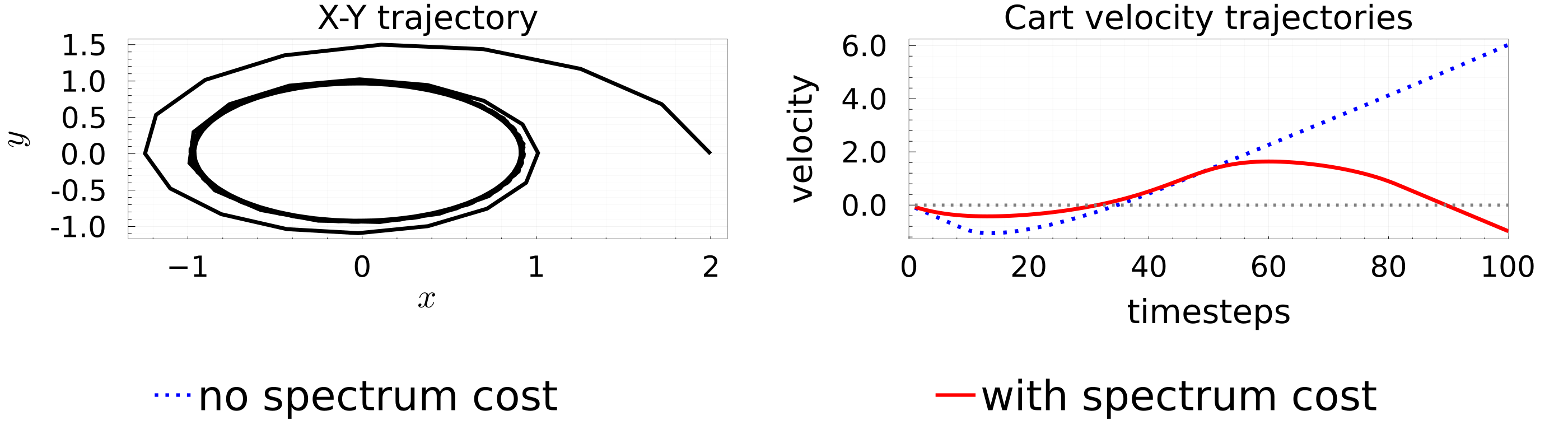
Figure 1: Left: We minimize solely for Koopman spectrum cost $\Lambda(\mathscr{A})=\|\mathbf{m}-\mathbf{m}^{\star}\|_{1}$ to imitate the top mode of a reference spectrum to recover a desired limit cycle behavior for the single-integrator system. Right: by regularizing the spectral radius of a Cartpole with a cumulative cost that favors high velocity, the cartpole performs a stable oscillation rather than moving off to infinity.

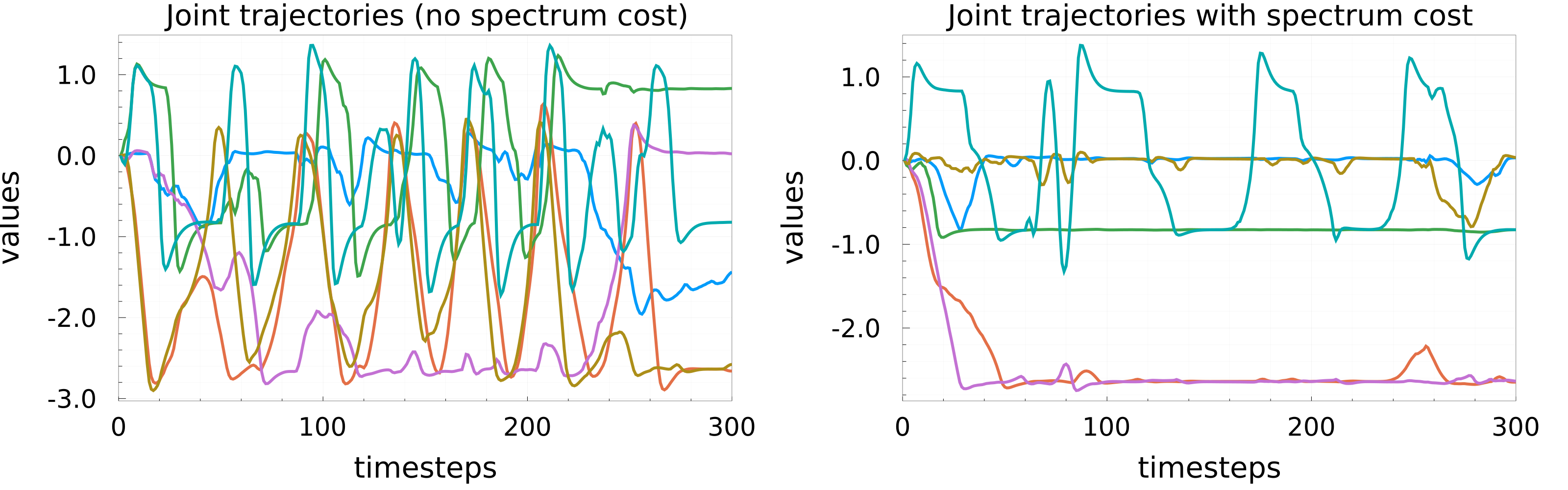
Figure 2: The joint angle trajectories generated by a combination of linear and RFF policies. Left: when only cumulative reward is maximized. Right: when both the cumulative cost and the spectrum cost $\Lambda(\mathscr{A})=5\sum_{i=1}^{d_{\phi}}|\lambda_{i}(\mathscr{A})|$ are used, where the factor $5$ is multiplied to balance between the spectrum cost and the cumulative cost.

Imitating target behaviors through the Koopman operators

We consider the limit cycle dynamics

$$\dot{r}=r(1-r^{2}),~{}\dot{\theta}=1,$$

described by the polar coordinates, and find the Koopman operator for this dynamics by sampling transitions, assuming $\mathcal{H}$ is the span of Random Fourier Features (RFFs) (Rahimi and Recht, 2007). With $\Pi$ a space of RFF policies that define $\dot{r}$ and $\dot{\theta}$ as a single-integrator model, we solve KSNR for the spectrum cost $\Lambda(\mathscr{A})=\|\mathbf{m}-\mathbf{m}^{\star}\|_{1}$, where $\mathbf{m}\in\mathbb{C}^{d_{\phi}}$ is the top mode (i.e., eigenvector of $\mathscr{A}$ corresponding to the largest absolute eigenvalue) and $\mathbf{m}^{\star}$ is the top mode of the target Koopman operator found previously, not the full spectrum. Figure 1 (Left) plots the trajectories (of the Cartesian coordinates) generated by RFF policies that minimizes this cost; it is observed that the agent successfully converged to the desired limit cycle of radius one by imitating the dominating mode of the target spectrum.

Generating stable loops (Cartpole)

We consider a Cartpole environment (where the rail length is extended from the original model). The single-step reward (negative cost) is $10^{-3}|v|$ where $v$ is the velocity of the cart, plus the penalty $-1$ when the pole falls down (i.e., directing downward). The additional spectrum cost considered in this experiment is $\Lambda(\mathscr{A})=10^{4}\max(1,\rho(\mathscr{A}))$, which highly penalizes spectral radius larger than one. Figure 1 (Right) plots the cart velocity trajectories generated by RFF policies that (approximately) solve KSNR with/without the spectrum cost. It is observed that spectral regularization led to a back-and-forth motion while the non-regularized policy preferred accelerating to one direction to solely maximize velocity. When the spectrum cost was used, the cumulative rewards were $0.072$ and the spectral radius was $0.990$, while they were $0.212$ and $1.003$ when the spectrum cost was not used; limiting the spectral radius prevents the ever increasing change in position.

Generating smooth movements (Walker)

We use the Walker2d environment and compare movements with/without the spectrum cost. The single-step reward (negative cost) is given by $v-0.001\|a\|^{2}_{\mathbb{R}^{6}}$, where $v$ is the velocity and $a$ is the action vector of dimension $6$. The spectrum cost is given by $\Lambda(\mathscr{A})=5\sum_{i=1}^{d_{\phi}}|\lambda_{i}(\mathscr{A})|$, where the factor $5$ is multiplied to balance between the spectrum and cumulative cost. Figure 2 plots typical joint angles along a trajectory generated by a combination of linear and RFF policies that (approximately) solves KSNR with/without the spectrum cost. It is observed that the spectrum cost led to simpler, smoother, and more periodic dynamics while doing the task sufficiently well. With the spectrum cost, the cumulative rewards and the spectrum costs averaged across four random seeds (plus-minus standard deviation) were $584\pm 112$ and $196\pm 8.13$. Without the spectrum cost, they were $698\pm 231$ and $310\pm 38.6$. Please also refer to Appendix G for detailed results.

4 Provably efficient algorithm for online KSNR

In this section, we present a learning algorithm for online KSNR. The learning goal is to find a parameter $\Theta^{\star t}$ that satisfies (3.2) at each episode $t\in[T]$. We employ episodic learning, and let $\Theta^{t}$ be a parameter employed at the $t$-th episode. Adversary chooses $X_{0}^{t}:=\{(x^{t}_{0,0},H^{t}_{0}),(x^{t}_{0,1},H^{t}_{1}),\ldots,(x^{t}_{0,N^{t}-1},H^{t}_{N^{t}-1})\}\subset\mathcal{X}\times\mathbb{Z}_{>0}$, where $N^{t}\in\mathbb{Z}_{>0}$, and the cost function $c^{t}$ at the beginning of the each episode. Let $c_{h,n}^{t}:=c^{t}(x^{t}_{h,n})$. $\omega\in\Omega_{\Theta^{t}}$ is chosen according to $P_{\Theta^{t}}$.

Algorithm evaluation.

In this work, we employ the following performance metric, namely, the regret:

$$\textsc{Regret}_{T}:=\sum_{t=0}^{T-1}\left(\Lambda[\mathscr{K}(\Theta^{t})]+\sum_{n=0}^{N^{t}-1}\sum_{h=0}^{H^{t}_{n}-1}c_{h,n}^{t}\right)-\sum_{t=0}^{T-1}\min_{\Theta\in\Pi}\left(\Lambda[\mathscr{K}(\Theta)]+J^{\Theta}(X_{0}^{t};c^{t})\right).$$

Below, we present model assumptions and an algorithm with a regret bound.

4.1 Models and algorithms

We make the following modeling assumptions.

Assumption 1.

Let $\mathscr{K}(\Theta)$ be the Koopman operator corresponding to a parameter $\Theta$. Then, assume that there exists a finite-dimensional subspace $\mathcal{H}_{0}$ on $\mathcal{X}$ over $\mathbb{R}$ and its basis $\phi_{1},\dots,\phi_{d_{\phi}}$ such that the random dynamical system (3.1) satisfies the following:

$$\forall\Theta\in\Pi,~{}\forall x\in\mathcal{X}:~{}\phi_{i}(\mathcal{F}^{\Theta}(1,\omega,x))=[\mathscr{K}(\Theta)\phi_{i}](x)+\epsilon_{i}(\omega),$$

where the additive noise $\epsilon_{i}(\omega)\sim\mathcal{N}(0,\sigma^{2})$ is assumed to be independent across timesteps, parameters $\Theta$, and indices $i$.

Assumption 2 (Function-valued RKHS (see Appendix A for details)).

$\mathscr{K}(\cdot)\phi$ for $\phi\in\mathcal{H}$ is assumed to live in a known function valued RKHS with the operator-valued reproducing kernel $K(\cdot,\cdot):\Pi\times\Pi\rightarrow\mathcal{L}(\mathcal{H};\mathcal{H})$, or equivalently, there exists a known map $\Psi:\Pi\rightarrow\mathcal{L}(\mathcal{H};\mathcal{H}^{\prime})$ for a specific Hilbert space $\mathcal{H}^{\prime}$ satisfying for any $\phi\in\mathcal{H}$, there exists $\psi\in\mathcal{H}^{\prime}$ such that

$$\mathscr{K}(\cdot)\phi=\Psi(\cdot)^{\dagger}\psi.$$ (4.1)

When 2 holds, we obtain the following claim which is critical for our learning framework.

Lemma 4.1.

Suppose Assumption 2 holds. Then, there exists a linear operator $M^{\star}:\mathcal{H}\rightarrow\mathcal{H}^{\prime}$ such that

$$\mathscr{K}(\Theta)=\Psi(\Theta)^{\dagger}\circ M^{\star}.$$

In the reminder of this paper, we work on the invariant subspace $\mathcal{H}_{0}$ in Assumption 1 and thus we regard $\mathcal{H}=\mathcal{H}_{0}\cong\mathbb{R}^{d_{\phi}}$, $\mathcal{L}(\mathcal{H};\mathcal{H})\cong\mathbb{R}^{d_{\phi}\times d_{\phi}}$, and, by abuse of notations, we view $\mathscr{K}(\Theta)$ as the realization of the operator over $\mathbb{R}^{d_{\phi}}$, i.e.,

$$\boldsymbol{\phi}_{\mathcal{F}^{\Theta}(1,\omega,x)}=\mathscr{K}(\Theta)\boldsymbol{\phi}_{x}+\epsilon(\omega)=[\Psi(\Theta)^{\dagger}\circ M^{\star}]\boldsymbol{\phi}_{x}+\epsilon(\omega),$$

where $\boldsymbol{\phi}_{x}:=[\phi_{1}(x),\phi_{2}(x),\ldots,\phi_{d_{\phi}}(x)]^{\top}\in\mathbb{R}^{d_{\phi}}$, and $\epsilon(\omega):=[\epsilon_{1}(\omega),\epsilon_{2}(\omega),\ldots,\epsilon_{d_{\phi}}(\omega)]^{\top}$.

Finally, we assume the following.

Assumption 3 (Realizability of costs).

For all $t$, the single-step cost $c^{t}$ is known and satisfies $c^{t}(x)=w^{t}(\boldsymbol{\phi}_{x})$ for some known map $w^{t}:\mathbb{R}^{d_{\phi}}\rightarrow\mathbb{R}_{\geq 0}$.

For later use, we define, for all $t\in[T]$, $n\in[N^{t}]$, and $h\in[H_{n}^{t}]$; $\mathscr{A}^{t}_{h,n}\in\mathcal{L}\left(\mathcal{L}(\mathcal{H};\mathcal{H}^{\prime});\mathcal{H}\right)$ and $\mathscr{B}^{t}\in\mathcal{L}\left(\mathcal{L}(\mathcal{H};\mathcal{H}^{\prime});\mathcal{L}(\mathcal{H};\mathcal{H})\right)$ by

$$\mathscr{A}^{t}_{h,n}(M)=\left[\Psi(\Theta^{t})^{\dagger}\circ M\right]\left(\boldsymbol{\phi}_{x_{h,n}^{t}}\right),~{}~{}~{}~{}~{}~{}~{}\mathscr{B}^{t}(M)=\Psi(\Theta^{t})^{\dagger}\circ M.$$

Remark 4.2 (Hilbert-Schmidt operators).

Both $\mathscr{A}^{t}_{h,n}$ and $\mathscr{B}^{t}$ are Hilbert-Schmidt operators because the ranges $\mathcal{H}$ and $\mathcal{L}(\mathcal{H};\mathcal{H})$ are of finite dimension. Note, in case $\mathcal{H}^{\prime}$ is finite, we obtain

$$\boldsymbol{\phi}_{\mathcal{F}^{\Theta}(1,\omega,x)}=\Psi(\Theta)^{\dagger}M^{\star}\boldsymbol{\phi}_{x}+\epsilon(\omega)=(\boldsymbol{\phi}_{x}^{\dagger}\otimes\Psi(\Theta)^{\dagger}){\rm vec}(M^{\star})+\epsilon(\omega),$$

where ${\rm vec}$ is the vectorization of matrix.

With these preparations in mind, our proposed information theoretic algorithm, which is an extension of LC³ to KSNR problem (estimating the true operator $M^{\star}$) is summarized in Algorithm 1.

1:Parameter set $\Pi$; regularizer $\lambda$

2:Initialize $\textsc{Ball}_{M}^{0}$ to be a set containing $M^{\star}$.

3:for $t=0\dots T-1$ do

4:     Adversary chooses $X^{t}_{0}$.

5:     $\Theta^{t},\hat{M}_{t}=\operatorname*{arg\,min}_{\Theta\in\Pi,~{}M\in\textsc{Ball}_{M}^{t}}\Lambda[\Psi(\Theta)^{\dagger}\circ M]+J^{\Theta}(X^{t}_{0};M;c^{t})$

6:     Under the dynamics $\mathcal{F}^{\Theta^{t}}$, sample transition data $\tau^{t}:=\{\tau^{t}_{n}\}_{n=0}^{N^{t}-1}$, where $\tau^{t}_{n}:=\{x^{t}_{h,n}\}_{h=0}^{H^{t}_{n}}$

7:     Update $\textsc{Ball}_{M}^{t+1}$.

8:end for

Algorithm 1 Koopman-Spectrum LC³ (KS-LC³)

This algorithm assumes the following oracle.

Definition 4.1 (Optimal parameter oracle).

Define the oracle, OptDynamics, that computes the minimization problem (3.2) for any $\mathscr{K}$, $X_{0}$, $\Lambda$ and $c^{t}$ satisfying Assumption 3.

4.2 Information theoretic regret bounds

Here, we present the regret bound analysis. To this end, we make the following assumptions.

Assumption 4.

The operator $\Lambda$ satisfies the following (modified) Hölder condition:

$$\exists L\in\mathbb{R}_{\geq 0},~{}\exists\alpha\in(0,1],~{}\forall\mathscr{A}\in\mathcal{L}\left(\mathcal{H},\mathcal{H}\right),~{}\forall\Theta\in\Pi,~{}$$

$$\left|\Lambda[\mathscr{A}]-\Lambda[\mathscr{K}(\Theta)]\right|\leq L\cdot\max{\left\{\left\|\mathscr{A}-\mathscr{K}(\Theta)\right\|^{2},\left\|\mathscr{A}-\mathscr{K}(\Theta)\right\|^{\alpha}\right\}}.$$

Further, we assume there exists a constant $\Lambda_{\rm max}\geq 0$ such that, for any $\Theta\in\Pi$ and for any $M\in\textsc{Ball}_{M}^{0}$,

$$\left|\Lambda[\Psi(\Theta)^{\dagger}\circ M]\right|\leq\Lambda_{\rm max}.$$

For example, for spectral radius $\rho$, the following proposition holds using the result from  (Song, 2002, Corollary 2.3).

Proposition 4.3.

Assume there exists a constant $\Lambda_{\rm max}\geq 0$ such that, for any $\Theta\in\Pi$ and for any $M\in\textsc{Ball}_{M}^{0}$, $\rho(\Psi(\Theta)^{\dagger}\circ M)\leq\Lambda_{\rm max}$. Let the Jordan condition number of $\mathscr{K}(\Theta)$ be the following:

$$\kappa:=\sup_{\Theta\in\Pi}{\inf_{\mathcal{Q}(\Theta)}{\left\{\|\mathcal{Q}(\Theta)\|\|\mathcal{Q}(\Theta)^{-1}\|:\mathcal{Q}(\Theta)^{-1}\mathscr{K}(\Theta)\mathcal{Q}(\Theta)=\mathscr{J}(\Theta)\right\}}},$$

where $\mathscr{J}(\Theta)$ is a Jordan canonical form of $\mathscr{K}(\Theta)$ transformed by a nonsingular matrix $\mathcal{Q}(\Theta)$. Also, let $m$ be the order of the largest Jordan block. Then, if $\kappa<\infty$, the cost $\Lambda(\mathscr{A})=\rho(\mathscr{A})$ satisfies the Assumption 4 for

$$L:=(1+\kappa)d_{\phi}^{2}(1+\sqrt{d_{\phi}-1}),~{}~{}~{}~{}\alpha=\frac{1}{m}.$$

Note when $\mathscr{K}(\Theta)$ is diagonalizable for all $\Theta$, $\alpha=1$.

Assumption 5.

For every $t$, adversary chooses $N^{t}$ trajectories such that $\{\boldsymbol{\phi}_{x_{0,n}^{t}}\}$ satisfies that the smallest eigenvalue of $\sum_{n=0}^{N^{t}-1}\boldsymbol{\phi}_{x_{0,n}^{t}}\boldsymbol{\phi}_{x_{0,n}^{t}}^{\dagger}$ is bounded below by some constant $C>0$. Also, there exists a constant $H\in\mathbb{Z}_{>0}$ such that for every $t$, $\sum_{n=0}^{N^{t}-1}H^{t}_{n}\leq H$.

Remark 4.4 (On Assumption 5).

In practice, user may wait to end an episode until a sufficient number of trajectories is collected in order for the assumption to hold. Note, this assumption does not preclude the necessity of exploration because the smallest eigenvalue of $\sum_{n=0}^{N^{t}-1}\sum_{h=0}^{H_{n}^{t}-1}{\mathscr{A}^{t}_{h,n}}^{\dagger}\mathscr{A}^{t}_{h,n}$ is in general not bounded below by a positive constant. We hope that this assumption can be relaxed by assuming the bounds on the norms of $\boldsymbol{\phi}_{x_{0,n}}$ and $\mathscr{K}(\Theta)$ and by using matrix Bernstein inequality under additive Gaussian noise assumption.

Lastly, the following assumption is the modified version of the one made in (Kakade et al., 2020).

Assumption 6.

[Modified version of Assumption 2 in (Kakade et al., 2020)] Assume there exists a constant $V_{\max}>0$ such that, for every $t$,

$$\sup_{\Theta\in\Pi}\,\sum_{n=0}^{N^{t}-1}\mathbb{E}_{\Omega_{\Theta}}\left[\left(\sum_{h=0}^{H^{t}_{n}-1}c^{t}(x_{h,n}^{t})\right)^{2}\ \bigg{|}\ \Theta,x_{0,n}^{t}\right]\leq V_{\max}.$$

Theorem 4.5.

Suppose Assumption 1 to 6 hold. Set $\lambda=\frac{\sigma^{2}}{\|M^{\star}\|^{2}}$. Then, there exists an absolute constant $C_{1}$ such that, for all $T$, KS-LC³(Algorithm 1) using OptDynamics enjoys the following regret bound:

$$\mathbb{E}_{\rm KS-LC\textsuperscript{3}}\left[\textsc{Regret}_{T}\right]\leq C_{1}(\tilde{d}_{T,1}+\tilde{d}_{T,2})T^{1-\frac{\alpha}{2}},$$

where

$$\tilde{d}_{T,1}^{2} :=(1+\gamma_{T,\mathscr{B}})\left[L^{2}(1+C^{-1})^{2}\tilde{\beta}_{2,T}+(L^{2}+\Lambda_{\rm max}L)(1+C^{-1})\tilde{\beta}_{1,T}+\Lambda_{\rm max}^{2}+L^{2}\right],$$

$$\tilde{d}_{T,2}^{2} :=\gamma_{T,\mathscr{A}}HV_{\max}\left(\gamma_{T,\mathscr{A}}+d_{\phi}+\log(T)+H\right),$$

$$\tilde{\beta}_{1,T} :=\sigma^{2}(d_{\phi}+\log(T)+\gamma_{T,\mathscr{A}}),$$

$$\tilde{\beta}_{2,T} :=\sigma^{4}((d_{\phi}+\log(T)+\gamma_{T,\mathscr{A}})^{2}+\gamma_{2,T,\mathscr{A}}).$$

Here, $\gamma_{T,\mathscr{A}}$, $\gamma_{2,T,\mathscr{A}}$, and $\gamma_{T,\mathscr{B}}$ are the expected maximum information gains that scale (poly-)logarithmically with $T$ under practical settings (see Appendix B for details).

Remark 4.6.

We note that, when $\alpha=1$, we obtain the order of $\tilde{O}(\sqrt{T})$.

4.3 Simulated experiments

We again consider a Cartpole environment for KS-LC³. To reduce the policy search space, we compose three pre-trained policies to balance the pole while 1) moving the cart position $p$ to $-0.3$ and then to $0.3$, 2) moving the cart with velocity $v=-1.5$, 3) moving cart with velocity $v=1.5$. We also extract the Koopman operator $\mathscr{A}^{\star}$ for the first policy. Then, we let $\Pi$ to be the space of linear combinations of the three policies, reducing the dimension of $\Theta$. We let the first four features $\phi_{1}(x)$ to $\phi_{4}(x)$ be $x_{1}$ to $x_{4}$, where $x=[x_{1},\ldots,x_{4}]^{\top}$ is the state, and the rest as RFFs.

The single-step cost is given by $10^{-4}(|v|-1.5)^{2}$ plus the large penalty when the pole falls down (i.e., directing downward), and the spectrum cost is $\Lambda(\mathscr{A})=\|\mathscr{A}[1:4,:]-\mathscr{A}^{\star}[1:4,:]\|^{2}_{HS}+0.01\sum_{i=1}^{d_{\phi}}|\lambda_{i}(\mathscr{A})|$, where $\mathscr{A}[1:4,:]\in\mathbb{R}^{4\times d_{\phi}}$ is the first four rows of $\mathscr{A}$; this imitates the first policy while also regularizing the spectrum.

When CEM is used to (approximately) solve KSNR, the resulting cart position trajectories are given by Figure 3 (Left). With the spectrum cost, the cumulative costs and the spectrum costs averaged across four random seeds were $0.706\pm 0.006$ and $2.706\pm 0.035$. Without the spectrum cost, they were $0.428\pm 0.045$ and $3.383\pm 0.604$.

We then use the Thompson sampling version of KS-LC³; the resulting cart position trajectories are given by Figure 3 (Left) as well, and the spectrum cost curve evaluated approximately using the current trajectory data is given in Figure 3 (Middle). Note the curve is averaged across four random seeds and across episode window of size four. Additionally, the estimated spectrum cost curve obtained by using the current estimate $\hat{M}$ is plotted in Figure 3 (Right). It is observed that the addition of the spectrum cost favored the behavior corresponding to the target Koopman operator to oscillate while balancing the pole, and achieved similar performance to the ground-truth model optimized with CEM.

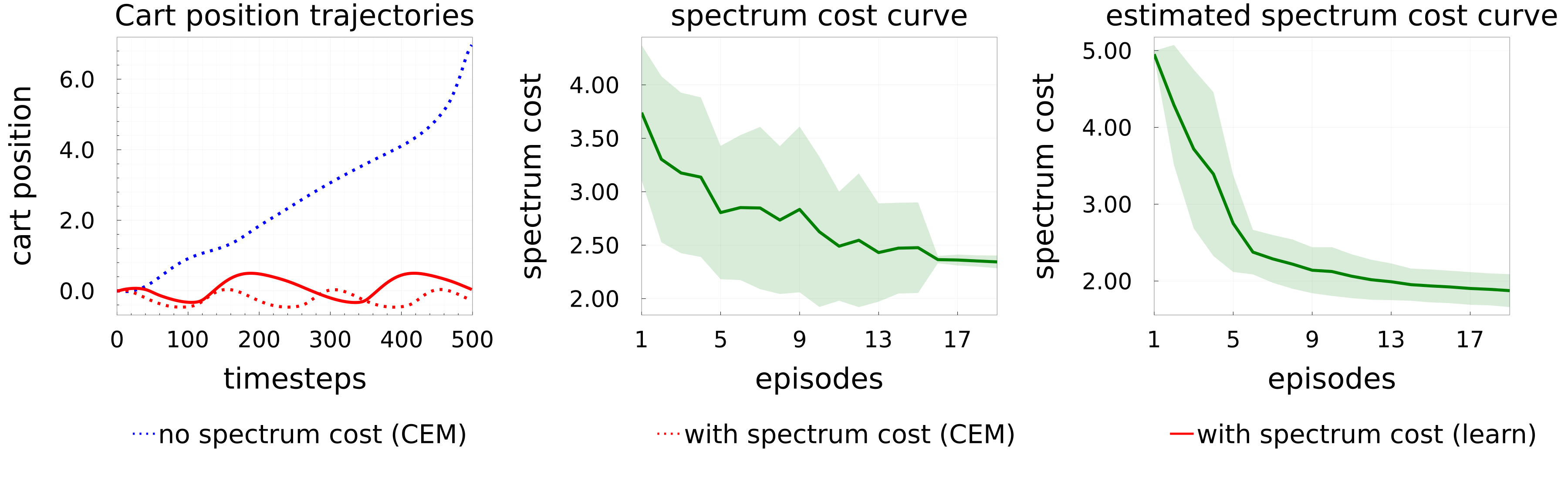
Figure 3: Cartpole imitation by KS-LC³ using the spectrum cost $\Lambda(\mathscr{A})=\|\mathscr{A}[1:4,:]-\mathscr{A}^{\star}[1:4,:]\|^{2}_{HS}+0.01\sum_{i=1}^{d_{\phi}}|\lambda_{i}(\mathscr{A})|$. Left: cart position trajectories with/without the spectrum cost with CEM on a known model versus the learned model with KS-LC³. Middle: the spectrum cost curve evaluated approximately using the current trajectory data. Right: the estimated spectrum cost curve obtained by using the current estimate $\hat{M}$.

5 Discussion and conclusion

This work proposed a novel paradigm of controlling dynamical systems, which we refer to as Koopman Spectrum Nonlinear Regulator, and presented information theoretic algorithm that achieves a sublinear regret bound under model assumptions. We showed that behaviors such as limit cycles of interest, stable periodic motion, and smooth movements are effectively realized within our framework. In terms of learning algorithms, we stress that there is a significant potential of future work for inventing sophisticated and scalable methods that elicit desired and interesting behaviors from dynamical systems. Our motivation of this work stems from the fact that some preferences over dynamical systems cannot be encoded by cumulative single-step cost based control/learning algorithms; we believe that this work enables a broader representation of dynamical properties that can enable more intelligent and robust agent behaviors.

6 Limitations

First, when the dynamical systems of interests do not meet certain conditions, Koopman operators might not be well defined over functional spaces that can be practically managed (e.g., RKHSs). Studying such conditions is an on-going research topic, and we will need additional studies of mis-specified cases where only an approximately invariant Koopman space is employed with errors.

Second, to solve KSNR, one needs heuristic approximations when the (policy) space $\Pi$ or the state space $\mathcal{X}$ is continuous. Even when the dynamical system model is known, getting better approximation results would require certain amount of computations, and additional studies on the relation between the amount of computations (or samples) and approximation errors would be required.

Third, KS-LC³ requires several assumptions for tractable regret analysis. It is again a somewhat strong assumption that one can find a Koopman invariant space $\mathcal{H}$. Further, additive Gaussian noise assumption may not be satisfied exactly in some practical applications, and robustness against the violations of the assumptions is an important future work. However, we stress that we believe the analysis of provably correct methods deepens our understandings of the problem.

Lastly, we note that our empirical experiment results are only conducted on simulators; to apply to real robotics problems, we need additional studies, such as computation-accuracy trade-off, safety/robustness issues, and simulation-to-real, if necessary. Also, balancing between cumulative cost and the Koopman spectrum cost is necessary to avoid unexpected negative outcomes.

7 Negative social impacts

The work, along with other robotics/control literature, encourages the further automation of robots; which would lead to loss of jobs that are currently existent, or lead to developments of harmful military robots. The more robots are automated, the more jobs may be replaced by robots, which would create new jobs such as robotics engineering for supervising AI algorithms, and insurance businesses for robot’s misbehavior. Also, when our proposed framework requires additional (computational or other) resources, it would benefit entities with larger amount of such resources.

Keeping in mind that KSNR does not necessarily guarantee the exact motion generations that humans expect, there is always a risk of robots misbehaving under partially unknown environments or under adversarial attacks; as pointed out in Section 6, unless mis-specified cases are sufficiently studied, our proposed framework would cause unexpected outcomes even in known environments. Also, we stress that the use of the Koopman spectrum cost has no implications on ”good” and ”bad” about any particular human behaviors.

To mitigate aforementioned negative impacts, further studies on mis-specified cases, safety, robustness, clearer relations between the costs and movements, and real robotics problems, in addition to feedback collections, are important.

Appendix A Function-valued RKHS

Function-valued reproducing kernel Hilbert spaces (RKHSs) are defined below.

Definition A.1 ([Kadri et al., 2016]).

A Hilbert space $(\mathcal{H}_{K},\left<\cdot,\cdot\right>_{\mathcal{H}_{K}})$ of functions from $\Pi$ to a Hilbert space $(\mathcal{H},\left<\cdot,\cdot\right>_{\mathcal{H}})$ is called a reproducing kernel Hilbert space if there is a nonnegative $\mathcal{L}(\mathcal{H};\mathcal{H})$-valued kernel $K$ on $\Pi\times\Pi$ such that:

1. $\Theta\mapsto K(\Theta^{\prime},\Theta)\phi$ belongs to $\mathcal{H}_{K}$ for all $\Theta^{\prime}\in\Pi$ and $\phi\in\mathcal{H}$,

2. for every $\mathscr{G}\in\mathcal{H}_{K},~{}\Theta\in\Pi$ and $\phi\in\mathcal{H}$, $\left<\mathscr{G},K(\Theta,\cdot)\phi\right>_{\mathcal{H}_{K}}=\left<\mathscr{G}(\Theta),\phi\right>_{\mathcal{H}}$.

For function-valued RKHSs, the following proposition holds.

Proposition A.1 (Feature map [Brault et al., 2016]).

Let $\mathcal{H}^{\prime}$ be a Hilbert space and $\Psi:\Pi\rightarrow\mathcal{L}(\mathcal{H};\mathcal{H}^{\prime})$. Then the operator $W:\mathcal{H}^{\prime}\rightarrow\mathcal{H}^{\Pi}$ defined by $[W\psi](\Theta):=\Psi(\Theta)^{\dagger}\psi,~{}\forall\psi\in\mathcal{H}^{\prime}$ and $~{}\forall\Theta\in\Pi$, is a partial isometry from $\mathcal{H}^{\prime}$ onto the reproducing kernel Hilbert space $\mathcal{H}_{K}$ with a reproducing kernel $K(\Theta_{2},\Theta_{1})=\Psi(\Theta_{2})^{\dagger}\Psi(\Theta_{1}),~{}~{}\forall\Theta_{1},\Theta_{2}\in\Pi$.

Remark A.2 (Decomposable kernel).

In practice, one can use decomposable kernel  [Brault et al., 2016]; When the kernel $K$ is given by $K(\Theta_{1},\Theta_{2})=k(\Theta_{1},\Theta_{2})A$ for some scalar-valued kernel $k(\Theta_{1},\Theta_{2})$ and for positive semi-definite operator $A\in\mathcal{L}(\mathcal{H},\mathcal{H})$, the kernel $K$ is called decomosable kernel. For an RKHS of a decomposable kernel $K$, (4.1) becomes

$$\mathscr{K}(\Theta)\phi=(\zeta(\Theta)^{\dagger}\otimes B)\psi,$$

where $\zeta:\Pi\rightarrow\mathcal{H}^{\prime\prime}$ is known ($\mathcal{H}^{\prime\prime}$ is some Hilbert space), and $A=BB^{\dagger}$. Further, to use RFFs, one considers a shift-invariant kernel $k(\Theta_{1},\Theta_{2})$.

Appendix B Some definitions of the values

The value $J^{\Theta}(X^{t}_{0};M;c^{t})$ in Algorithm 1 is defined by

$$J^{\Theta}(X^{t}_{0};M;c^{t}):=\sum_{n=0}^{N^{t}-1}\mathbb{E}_{\Omega_{\Theta}}\left[\sum_{h=0}^{H^{t}_{n}-1}c^{t}(x^{t}_{h,n})\Big{|}\Theta,M,x^{t}_{0,n}\right],$$

where the expectation is taken over the trajectory following $\boldsymbol{\phi}_{x_{h+1}}=[\Psi(\Theta)^{\dagger}\circ M]\boldsymbol{\phi}_{x}+\epsilon(\omega)$. Also the confidence balls at time instance $t$ is given by

$$\textsc{Ball}_{M}^{t}:=\left\{M\bigg{|}\left\|(\Sigma_{\mathscr{A}}^{t})^{\frac{1}{2}}\left(M-\overline{M}^{t}\right)\right\|^{2}\leq\beta_{M}^{t}\right\}\cap\textsc{Ball}_{M}^{0},~{}~{}\Sigma_{\mathscr{A}}^{t}:=\lambda I+\sum_{\tau=0}^{t-1}\sum_{n=0}^{N^{\tau}-1}\sum_{h=0}^{H^{\tau}_{n}-1}{\mathscr{A}^{\tau}_{h,n}}^{\dagger}{\mathscr{A}^{\tau}_{h,n}},$$

and $\Sigma_{\mathscr{A}}^{0}:=\lambda I$, where $\beta_{M}^{t}:=20\sigma^{2}\left(d_{\phi}+\log\left(t\frac{\det(\Sigma_{\mathscr{A}}^{t})}{\det(\Sigma_{\mathscr{A}}^{0})}\right)\right)$ and

$$\overline{M}^{t}:=\operatorname*{arg\,min}_{M}\left[\sum_{\tau=0}^{t-1}\sum_{n=0}^{N^{\tau}-1}\sum_{h=0}^{H^{\tau}_{n}-1}\left\|\boldsymbol{\phi}_{x^{\tau}_{h+1,n}}-\mathscr{A}^{\tau}_{h,n}(M)\right\|_{\mathbb{R}^{d_{\phi}}}^{2}+\lambda\left\|M\right\|_{\rm HS}^{2}\right].$$

Similar to the work [Kakade et al., 2020], we define the expected maximum information gains as:

$$\gamma_{T,\mathscr{A}}(\lambda):=2\max_{\mathcal{A}}\mathbb{E}_{\mathcal{A}}\left[\log\left(\frac{\det\left(\Sigma_{\mathscr{A}}^{T}\right)}{\det\left(\Sigma_{\mathscr{A}}^{0})\right)}\right)\right].$$

Here, $\det$ is a properly defined functional determinant of a bounded linear operator. Further,

$$\gamma_{2,T,\mathscr{A}}(\lambda):=2\max_{\mathcal{A}}\mathbb{E}_{\mathcal{A}}\left[\left(\log\left(\frac{\det\left(\Sigma_{\mathscr{A}}^{T}\right)}{\det\left(\Sigma_{\mathscr{A}}^{0})\right)}\right)\right)^{2}\right].$$

Also, we define

$$\Sigma_{\mathscr{B}}^{t}:=\lambda I+\sum_{\tau=0}^{t-1}{\mathscr{B}^{t}}^{\dagger}\mathscr{B}^{t},~{}~{}~{}\Sigma_{\mathscr{B}}^{0}:=\lambda I,~{}~{}\gamma_{T,\mathscr{B}}(\lambda):=2\max_{\mathcal{A}}\mathbb{E}_{\mathcal{A}}\left[\log\left(\frac{\det\left(\Sigma_{\mathscr{B}}^{T}\right)}{\det\left(\Sigma_{\mathscr{B}}^{0})\right)}\right)\right].$$

Lemma B.1.

Assume that $\Psi(\Theta)\in\mathbb{R}^{d_{\Psi}\times d_{\phi}}$ and that $\|\mathscr{B}^{t}\|_{\rm HS}\leq B_{\mathscr{B}},~{}\|\mathscr{A}^{t}_{h,n}\|_{\rm HS}\leq B_{\mathscr{A}}$ for all $t\in[T]$, $n\in[N^{t}]$, and $h\in[H^{t}_{n}]$ and some $B_{\mathscr{B}}\geq 0$ and $B_{\mathscr{A}}\geq 0$. Then, $\gamma_{T,\mathscr{A}}(\lambda)=O(d_{\phi}d_{\Psi}\log(1+THB_{\mathscr{A}}^{2}/\lambda))$, and $\gamma_{T,\mathscr{B}}(\lambda)=O(d_{\phi}d_{\Psi}\log(1+TB_{\mathscr{B}}^{2}/\lambda)))$.

Proof.

For $\gamma_{T,\mathscr{A}}(\lambda)$, from the definition of Hilbert-Schmidt norm, we have

$$\mathrm{tr}{\left(\sum_{t=0}^{T-1}\sum_{n=0}^{N^{t}-1}\sum_{h=0}^{H^{t}_{n}-1}{\mathscr{A}^{t}_{h,n}}^{\dagger}{\mathscr{A}^{t}_{h,n}}\right)}\leq THB_{\mathscr{A}}^{2},$$

and the result follows from  [Kakade et al., 2020, Lemma C.5]. The similar argument holds for $\gamma_{T,\mathscr{B}}(\lambda)$ too. ∎

Appendix C Formal argument on the limitation of cumulative costs

In this section, we present a formal argument on the limitation of cumulative costs, mentioned in Section 3.2. To this end, we give the following proposition.

Proposition C.1.

Let $\mathcal{X}=\mathbb{R}$. Consider the set $\mathcal{S}_{f}$ of dynamics converging to some point in $\mathcal{X}$. Then, for any choice of $\upsilon\in(0,1]$, set-valued map $\mathscr{S}:\mathcal{X}\rightarrow 2^{\mathcal{X}}\setminus\emptyset$, and cost $\mathbf{c}$ of the form

$$\mathbf{c}(x,y)=\begin{cases}0&(y\in\mathscr{S}(x)),\\ 1&({\rm otherwise}),\end{cases}$$

we have $\{\mathcal{F}\}\neq\mathcal{S}_{f}$. Here, $\{\mathcal{F}\}$ are given by

$$\bigcap_{x_{0}\in\mathcal{X}}\left\{\operatorname*{arg\,min}_{\mathcal{F}\text{\rm:r.d.s.}}\mathbb{E}_{\Omega}\sum_{h=0}^{\infty}\upsilon^{h}\mathbf{c}\left(\mathcal{F}(h,\omega,x_{0}),\mathcal{F}(h+1,\omega,x_{0})\right)\right\}.$$

Proof.

Assume there exist $\upsilon$, a set-valued map $\mathscr{S}$, and $\mathbf{c}$ such that the set $\{\mathcal{F}^{\Theta}\}=\mathcal{S}_{f}$. Then, because $\mathcal{S}_{f}$ is strictly smaller than the set of arbitrary dynamics, it must be the case that $\exists x_{0}\in\mathcal{X},~{}\exists y_{0}\in\mathcal{X},~{}~{}y_{0}\notin\mathscr{S}(x_{0})$. However, the dynamics $f^{\star}$, where $f^{\star}(x_{0})=y_{0}$ and $f^{\star}(x)=x,~{}\forall x\in\mathcal{X}\setminus\{x_{0}\}$, is an element of $\mathcal{S}_{f}$. Therefore, the proposition is proved. ∎

Appendix D Proof of Lemma 4.1

It is easy to see that one can define a map $M_{0}$ so that it satisfies $M_{0}(\phi)=\psi$ such that Assumption 2 holds. Define

$$M^{\star}:=PM_{0},$$

where $P$ is the orthogonal projection operator onto the sum space of the orthogonal complement of the null space of $\Psi(\Theta)^{\dagger}$ for all $\Theta\in\Pi$, namely,

$$\overline{\sum_{\Theta\in\Pi}{\rm ker}(\Psi(\Theta)^{\dagger})^{\perp}}.$$

Also, define $P_{\Theta}$ by the orthogonal projection onto

$${\rm ker}(\Psi(\Theta)^{\dagger})^{\perp}.$$

Then, for any $\Theta\in\Pi$, we obtain

$$P_{\Theta}M_{0}={\Psi(\Theta)^{\dagger}}^{+}\mathscr{K}(\Theta),$$

where $\mathscr{A}^{+}$ is the pseudoinverse of the operator $\mathscr{A}$, and $P_{\Theta}M_{0}$ is linear. Let $a,b\in\mathbb{R}$ and $\phi_{1},\phi_{2}\in\mathcal{H}$, and define $\tilde{\psi}$ by

$$\tilde{\psi}:=PM_{0}(a\phi_{1}+b\phi_{2})-aPM_{0}(\phi_{1})-bPM_{0}(\phi_{2}).$$

Because $P_{\Theta}PM_{0}=P_{\Theta}M_{0}$, it follows that $P_{\Theta}\tilde{\psi}=0$ for all $\Theta\in\Pi$, which implies

$$\tilde{\psi}\in\bigcap_{\Theta\in\Pi}{\rm ker}P_{\Theta}=\bigcap_{\Theta\in\Pi}{\rm ker}(\Psi(\Theta)^{\dagger}).$$

On the other hand, we have

$$\tilde{\psi}\in\overline{\sum_{\Theta\in\Pi}{\rm ker}(\Psi(\Theta)^{\dagger})^{\perp}}.$$

Therefore, it follows that $\tilde{\psi}=0$, which proves that $M^{\star}$ is linear.

Appendix E Proof of Proposition 4.3

Fix $\Theta\in\Pi$ and suppose that the eigenvalues $\lambda_{i}$ ($i\in\mathcal{I}:=\{1,2,\ldots,d_{\phi}\}$) of $\mathscr{K}(\Theta)$ are in descending order according to their absolute values, i.e., $|\lambda_{1}|\geq|\lambda_{2}|\geq\ldots\geq|\lambda_{d_{\phi}}|$. Given $\mathscr{A}\in\mathcal{L}(\mathcal{H};\mathcal{H})$, suppose also that the eigenvalues $\mu_{i}$ ($i\in\mathcal{I}$) of $\mathscr{A}$ are in descending order according to their absolute values. Let

$$\kappa_{\Theta}:={\inf_{\mathcal{Q}(\Theta)}{\left\{\|\mathcal{Q}(\Theta)\|\|\mathcal{Q}(\Theta)^{-1}\|:\mathcal{Q}(\Theta)^{-1}\mathscr{K}(\Theta)\mathcal{Q}(\Theta)=\mathscr{J}(\Theta)\right\}}},$$

where $\mathscr{J}(\Theta)$ is a Jordan canonical form of $\mathscr{K}(\Theta)$ transformed by a nonsingular matrix $\mathcal{Q}(\Theta)$. Also, let

$$\overline{\kappa}_{\Theta}:=\max_{m\in\{1,\ldots,d_{\phi}\}}\left\{\kappa_{\Theta}^{\frac{1}{m}}\right\}.$$

Then, by [Song, 2002, Corollary 2.3], we have

$$||\mu_{i}|-|\lambda_{i}||\leq|\mu_{i}-\lambda_{i}|\leq\sum_{i}|\mu_{i}-\lambda_{i}|\leq\sum_{i}|\mu_{\pi(i)}-\lambda_{i}|$$

$$\leq d_{\phi}\sqrt{d_{\phi}}(1+\sqrt{d_{\phi}-p})\max\left\{\kappa_{\Theta}\sqrt{d_{\phi}}\|\mathscr{A}-\mathscr{K}(\Theta)\|,(\kappa_{\Theta}\sqrt{d_{\phi}})^{\frac{1}{m}}\|\mathscr{A}-\mathscr{K}(\Theta)\|^{\frac{1}{m}}\right\},$$

for any $i\in\mathcal{I}$ and for some permutation $\pi$, where $p\in\{1,2,\ldots,d_{\phi}\}$ is the number of the Jordan block of $\mathcal{Q}(\Theta)^{-1}\mathscr{K}(\Theta)\mathcal{Q}(\Theta)$ and $m\in\{1,2,\ldots,d_{\phi}\}$ is the order of the largest Jordan block. Because $\sqrt{d_{\phi}-p}\leq\sqrt{d_{\phi}-1}$ for any $p\in\{1,2,\ldots,d_{\phi}\}$, and because

$$\max_{m\in\{1,\ldots,d_{\phi}\}}\left[\sqrt{d_{\phi}}\cdot\max\{\sqrt{d_{\phi}},(\sqrt{d_{\phi}})^{\frac{1}{m}}\}\cdot\max\left\{\kappa_{\Theta},\kappa_{\Theta}^{\frac{1}{m}}\right\}\right]\leq d_{\phi}\overline{\kappa}_{\Theta},$$

it follows that

$$|\rho(\mathscr{A})-\rho(\mathscr{K}(\Theta))|=||\mu_{1}|-|\lambda_{1}||$$

$$\leq\overline{\kappa}_{\Theta}d_{\phi}^{2}(1+\sqrt{d_{\phi}-1})\max\left\{\|\mathscr{A}-\mathscr{K}(\Theta)\|,\|\mathscr{A}-\mathscr{K}(\Theta)\|^{1/m}\right\}.$$

Since $\overline{\kappa}_{\Theta}<1+\kappa$, simple computations complete the proof.

Appendix F Regret analysis

Throughout this section, suppose Assumptions 1 to 6 hold. Note that Assumption 3 is required for OptDynamics. We first give the following lemmas.

Lemma F.1.

Let $\mathcal{H}$ be a Hilbert space and $A_{i},~{}B_{i}\in\mathcal{L}(\mathcal{H};\mathcal{H})~{}(i\in\{1,2,\ldots,n\})$. Assume, for all $i\in\{1,2,\ldots,n\}$, that $A_{i}$ is positive definite. Also, assume $B_{1}$ is positive definite, and for all $i\in\{2,3,\ldots,n\}$, $B_{i}$ is positive semi-definite. Then,

$$\left\|\left(\sum_{i}B^{\frac{1}{2}}_{i}A_{i}B^{\frac{1}{2}}_{i}\right)^{-\frac{1}{2}}\left(\sum_{i}B_{i}\right)\left(\sum_{i}B^{\frac{1}{2}}_{i}A_{i}B^{\frac{1}{2}}_{i}\right)^{-\frac{1}{2}}\right\|\leq\max_{i}\left\|A_{i}^{-1}\right\|.$$

If $A_{i}B_{i}=B_{i}A_{i}$ for all $i\in\{1,2,\ldots,n\}$, then

$$\left\|\left(\sum_{i}A_{i}B_{i}\right)^{-\frac{1}{2}}\left(\sum_{i}B_{i}\right)\left(\sum_{i}A_{i}B_{i}\right)^{-\frac{1}{2}}\right\|\leq\max_{i}\left\|A_{i}^{-1}\right\|.$$

Proof.

Let $c:=\max_{i}\left\|A_{i}^{-1}\right\|$. Then, we have, for all $i$,

$$I\preceq\left\|A_{i}^{-1}\right\|A_{i}\preceq cA_{i},$$

from which it follows that

$$B_{i}\preceq cB^{\frac{1}{2}}_{i}A_{i}B^{\frac{1}{2}}_{i}.$$

Therefore, we obtain

$$\sum_{i}B_{i}\preceq c\sum_{i}B^{\frac{1}{2}}_{i}A_{i}B^{\frac{1}{2}}_{i}.$$

From the assumptions, $\left(\sum_{i}B^{\frac{1}{2}}_{i}A_{i}B^{\frac{1}{2}}_{i}\right)^{-1}$ exists and

$$\left(\sum_{i}B^{\frac{1}{2}}_{i}A_{i}B^{\frac{1}{2}}_{i}\right)^{-\frac{1}{2}}\left(\sum_{i}B_{i}\right)\left(\sum_{i}B^{\frac{1}{2}}_{i}A_{i}B^{\frac{1}{2}}_{i}\right)^{-\frac{1}{2}}\preceq cI,$$

from which we obtain

$$\left\|\left(\sum_{i}B^{\frac{1}{2}}_{i}A_{i}B^{\frac{1}{2}}_{i}\right)^{-\frac{1}{2}}\left(\sum_{i}B_{i}\right)\left(\sum_{i}B^{\frac{1}{2}}_{i}A_{i}B^{\frac{1}{2}}_{i}\right)^{-\frac{1}{2}}\right\|\leq c.$$

The second claim follows immediately. ∎

Lemma F.2.

Suppose Assumptions 1, 2, and 5 hold. Then, it follows that, for all $t\in[T]$,

$$\left\|(\Sigma_{\mathscr{B}}^{t})^{\frac{1}{2}}\left(M-{\overline{M}^{t}}\right)\right\|^{2}\leq(1+C^{-1})\left\|(\Sigma_{\mathscr{A}}^{t})^{\frac{1}{2}}\left(M-\overline{M}^{t}\right)\right\|^{2}.$$

Proof.

Under Assumptions 1 and 2, define $\mathscr{C}^{t}\in\mathcal{L}\left(\mathcal{L}(\mathcal{H};\mathcal{H}^{\prime});\mathcal{L}(\mathcal{H};\mathcal{H}^{\prime})\right)$ by

$$\mathscr{C}^{t}(M)=M\circ\left[\sum_{n=0}^{N^{t}-1}\sum_{h=0}^{H^{t}_{n}-1}\boldsymbol{\phi}_{x^{t}_{h,n}}\boldsymbol{\phi}_{x^{t}_{h,n}}^{\dagger}\right].$$

Also, define $\mathscr{X}^{t}:=\sum_{n=0}^{N^{t}-1}\sum_{h=0}^{H^{t}_{n}-1}{\mathscr{A}_{h,n}^{t}}^{\dagger}\mathscr{A}_{h,n}^{t}$ and $\mathscr{Y}^{t}:={\mathscr{B}^{t}}^{\dagger}\mathscr{B}^{t}$. We have $\mathscr{C}^{t}\mathscr{Y}^{t}=\mathscr{Y}^{t}\mathscr{C}^{t}=\mathscr{X}^{t}$ (and thus $\mathscr{X}^{t}\mathscr{Y}^{t}=\mathscr{Y}^{t}\mathscr{X}^{t}$), and

$$\Sigma_{\mathscr{A}}^{t}=\lambda I+\sum_{\tau=0}^{t-1}\mathscr{X}^{\tau},~{}~{}~{}~{}~{}\Sigma_{\mathscr{B}}^{t}=\lambda I+\sum_{\tau=0}^{t-1}\mathscr{Y}^{\tau}.$$

From Assumption 5, we obtain, for all $t\in[T]$, $(\mathscr{C}^{t})^{-1}$ exists and

$$\|{(\mathscr{C}^{t})}^{-1}\|\leq\left\|\left(\sum_{n=0}^{N^{t}-1}\sum_{h=0}^{H^{t}_{n}-1}\boldsymbol{\phi}_{x^{t}_{h,n}}\boldsymbol{\phi}_{x^{t}_{h,n}}^{\dagger}\right)^{-1}\right\|\leq\left\|\left(\sum_{n=0}^{N^{t}-1}\boldsymbol{\phi}_{x_{0,n}^{t}}\boldsymbol{\phi}_{x_{0,n}^{t}}^{\dagger}\right)^{-1}\right\|\leq C^{-1}.$$

Therefore, using Lemma F.1 by substituting $I$ and $\mathscr{C}$ to $A$, $\lambda I$ and $\mathscr{Y}$ to $B$, it follows that

$$\left\|(\Sigma_{\mathscr{A}}^{t})^{-\frac{1}{2}}\Sigma_{\mathscr{B}}^{t}(\Sigma_{\mathscr{A}}^{t})^{-\frac{1}{2}}\right\|\leq\max\left\{1,\max_{\tau\in[t]}\{\|{(\mathscr{C}^{\tau})}^{-1}\|\}\right\}\leq 1+C^{-1},$$

and

$$\left\|(\Sigma_{\mathscr{B}}^{t})^{\frac{1}{2}}\left(M-{\overline{M}^{t}}\right)\right\|^{2}=\left\|(\Sigma_{\mathscr{B}}^{t})^{\frac{1}{2}}(\Sigma_{\mathscr{A}}^{t})^{-\frac{1}{2}}(\Sigma_{\mathscr{A}}^{t})^{\frac{1}{2}}\left(M-{\overline{M}^{t}}\right)\right\|^{2}$$

$$\leq\left\|(\Sigma_{\mathscr{A}}^{t})^{\frac{1}{2}}\left(M-\overline{M}^{t}\right)\right\|^{2}\left\|(\Sigma_{\mathscr{A}}^{t})^{-\frac{1}{2}}(\Sigma_{\mathscr{B}}^{t})^{\frac{1}{2}}\right\|^{2}=\left\|(\Sigma_{\mathscr{A}}^{t})^{-\frac{1}{2}}\Sigma_{\mathscr{B}}^{t}(\Sigma_{\mathscr{A}}^{t})^{-\frac{1}{2}}\right\|\left\|(\Sigma_{\mathscr{A}}^{t})^{\frac{1}{2}}\left(M-\overline{M}^{t}\right)\right\|^{2}$$

$$\leq(1+C^{-1})\left\|(\Sigma_{\mathscr{A}}^{t})^{\frac{1}{2}}\left(M-\overline{M}^{t}\right)\right\|^{2}.$$

Here, the second equality used $\|\mathscr{A}\|^{2}=\|\mathscr{A}\mathscr{A}^{\dagger}\|$. ∎

Now, let $\mathcal{E}^{t}$ be the event $M^{\star}\in\textsc{Ball}_{M}^{t}$. Assume $\bigcap_{t=0}^{T-1}\mathcal{E}^{t}$. Then, using Assumption 4,

$$\left(\Lambda[\mathscr{K}(\Theta^{t})]+J^{\Theta^{t}}(X^{t}_{0};c^{t})\right)-\left(\Lambda[\mathscr{K}(\Theta^{\star t})]+J^{\Theta^{\star t}}(X^{t}_{0};c^{t})\right)$$

$$=\left(\Lambda[\mathscr{K}(\Theta^{t})]-\Lambda[\mathscr{K}(\Theta^{\star t})]\right)+\left(J^{\Theta^{t}}(X^{t}_{0};c^{t})-J^{\Theta^{\star t}}(X^{t}_{0};c^{t})\right)$$

$$\leq\left(\Lambda[\mathscr{K}(\Theta^{t})]-\Lambda[\mathscr{B}_{t}\circ\hat{M}^{t}]\right)+\left(J^{\Theta^{t}}(X^{t}_{0};c^{t})-J^{\Theta^{t}}\left(X^{t}_{0};\hat{M}^{t};c^{t}\right)\right)$$

$$\leq\left(\left|\Lambda[\mathscr{K}(\Theta^{t})]-\Lambda[\mathscr{B}_{t}\circ\hat{M}^{t}]\right|\right)+\left(J^{\Theta^{t}}(X^{t}_{0};c^{t})-J^{\Theta^{t}}\left(X^{t}_{0};\hat{M}^{t};c^{t}\right)\right)$$

$$\leq\underbrace{\min\left\{L\cdot\max{\left\{\left\|\mathscr{B}_{t}\left(M^{\star}-\hat{M}^{t}\right)\right\|^{2},\left\|\mathscr{B}_{t}\left(M^{\star}-\hat{M}^{t}\right)\right\|^{\alpha}\right\}},2\Lambda_{\rm max}\right\}}_{\rm term_{1}}+\underbrace{\left(J^{\Theta^{t}}(X^{t}_{0};c^{t})-J^{\Theta^{t}}\left(X^{t}_{0};\hat{M}^{t};c^{t}\right)\right)}_{\rm term_{2}}.$$ (F.1)

Here, the first inequality follows because we assumed $\mathcal{E}^{t}$ and because the algorithm selects $\hat{M}^{t}$ and $\Theta^{t}$ such that

$$\Lambda[\mathscr{B}_{t}\circ\hat{M}^{t}]+J^{\Theta^{t}}\left(X^{t}_{0};\hat{M}^{t};c^{t}\right)\leq\Lambda[\mathscr{B}_{t}\circ M]+J^{\Theta}\left(X^{t}_{0};M;c^{t}\right)$$

for any $M\in\textsc{Ball}_{M}^{t}$ and for any $\Theta\in\Pi$. The third inequality follows from Assumption 4.

Using Lemma F.2, we have

$$\left\|\mathscr{B}_{t}\left({M^{\star}}-{\hat{M}^{t}}\right)\right\|\leq\left\|(\Sigma_{\mathscr{B}}^{t})^{\frac{1}{2}}\left({M^{\star}}-{\hat{M}^{t}}\right)\right\|\left\|\mathscr{B}_{t}(\Sigma_{\mathscr{B}}^{t})^{-\frac{1}{2}}\right\|$$

$$\leq\sqrt{(1+C^{-1})}\left\|(\Sigma_{\mathscr{A}}^{t})^{\frac{1}{2}}\left(M^{\star}-\hat{M}^{t}\right)\right\|\left\|\mathscr{B}_{t}(\Sigma_{\mathscr{B}}^{t})^{-\frac{1}{2}}\right\|$$

$$\leq\sqrt{(1+C^{-1})}\left(\left\|(\Sigma_{\mathscr{A}}^{t})^{\frac{1}{2}}\left(M^{\star}-\overline{M}^{t}\right)\right\|+\left\|(\Sigma_{\mathscr{A}}^{t})^{\frac{1}{2}}\left(\overline{M}^{t}-\hat{M}^{t}\right)\right\|\right)\left\|\mathscr{B}_{t}(\Sigma_{\mathscr{B}}^{t})^{-\frac{1}{2}}\right\|$$

$$\leq 2\sqrt{(1+C^{-1})\beta_{M}^{t}}\left\|\mathscr{B}_{t}(\Sigma_{\mathscr{B}}^{t})^{-\frac{1}{2}}\right\|~{}~{}~{}~{}~{}(\because\mathcal{E}^{t}).$$

Therefore, if $\mathcal{E}^{t}$, it follows that

$${\rm term_{1}}\leq\min\left\{L\left\{4(1+C^{-1})\beta_{M}^{t}+1\right\}\max\left\{\left\|\mathscr{B}_{t}(\Sigma_{\mathscr{B}}^{t})^{-\frac{1}{2}}\right\|^{2},\left\|\mathscr{B}_{t}(\Sigma_{\mathscr{B}}^{t})^{-\frac{1}{2}}\right\|^{\alpha}\right\},2\Lambda_{\rm max}\right\}.$$ (F.2)

Then, we use the following lemma which is an extension of  [Kakade et al., 2020, Lemman B.6] to our Hölder condition.

Lemma F.3.

For any sequence of $\mathscr{B}_{t}$ and for any $\alpha\in(0,1]$, we have

$$\sum_{t=0}^{T-1}\min\left\{\left\|\mathscr{B}_{t}(\Sigma_{\mathscr{B}}^{t})^{-\frac{1}{2}}\right\|^{2\alpha},1\right\}\leq 2T^{1-\alpha}\left[1+\log\left(\frac{\det\left(\Sigma_{\mathscr{B}}^{T}\right)}{\det\left(\Sigma_{\mathscr{B}}^{0}\right)}\right)\right].$$

Proof.

Using $x\leq 2\log(1+x)$ for $x\in[0,1]$,

$$\sum_{t=0}^{T-1}\min\left\{\left\|\mathscr{B}_{t}(\Sigma_{\mathscr{B}}^{t})^{-\frac{1}{2}}\right\|^{2\alpha},1\right\}\leq\sum_{t=0}^{T-1}\min\left\{\left\|\mathscr{B}_{t}(\Sigma_{\mathscr{B}}^{t})^{-\frac{1}{2}}\right\|_{\rm HS}^{2\alpha},1\right\}~{}~{}(\because\|\mathscr{A}\|\leq\|\mathscr{A}\|_{\rm HS})$$

$$=\sum_{t=0}^{T-1}\left(\min\left\{\left\|\mathscr{B}_{t}(\Sigma_{\mathscr{B}}^{t})^{-\frac{1}{2}}\right\|_{\rm HS}^{2},1\right\}\right)^{\alpha}\leq\sum_{t=0}^{T-1}\left[2\log{\left(1+\left\|\mathscr{B}_{t}(\Sigma_{\mathscr{B}}^{t})^{-\frac{1}{2}}\right\|_{\rm HS}^{2}\right)}\right]^{\alpha}$$

$$=\sum_{t=0}^{T-1}\left[2\log{\left(1+{\mathrm{tr}{\left\{(\Sigma_{\mathscr{B}}^{t})^{-\frac{1}{2}}\mathscr{B}_{t}^{\dagger}\mathscr{B}_{t}(\Sigma_{\mathscr{B}}^{t})^{-\frac{1}{2}}\right\}}}\right)}\right]^{\alpha}$$

$$\leq 2^{\alpha}\sum_{t=0}^{T-1}\left[\log\det{\left(I+(\Sigma_{\mathscr{B}}^{t})^{-\frac{1}{2}}\mathscr{B}_{t}^{\dagger}\mathscr{B}_{t}(\Sigma_{\mathscr{B}}^{t})^{-\frac{1}{2}}\right)}\right]^{\alpha}$$

$$\leq 2^{\alpha}T^{1-\alpha}\left[\sum_{t=0}^{T-1}\log\det{\left(I+(\Sigma_{\mathscr{B}}^{t})^{-\frac{1}{2}}\mathscr{B}_{t}^{\dagger}\mathscr{B}_{t}(\Sigma_{\mathscr{B}}^{t})^{-\frac{1}{2}}\right)}\right]^{\alpha}$$

$$\leq 2^{\alpha}T^{1-\alpha}\left[\sum_{t=0}^{T-1}\left(\log\det\left(\Sigma_{\mathscr{B}}^{t+1}\right)-\log\det\left(\Sigma_{\mathscr{B}}^{t}\right)\right)\right]^{\alpha}\leq 2T^{1-\alpha}\left[\log\left(\frac{\det\left(\Sigma_{\mathscr{B}}^{T}\right)}{\det\left(\Sigma_{\mathscr{B}}^{0}\right)}\right)\right]^{\alpha}$$

$$\leq 2T^{1-\alpha}\left(1+\log\left(\frac{\det\left(\Sigma_{\mathscr{B}}^{T}\right)}{\det\left(\Sigma_{\mathscr{B}}^{0}\right)}\right)\right).$$

∎

Here, the fifth inequality follows from  [Grafakos, 2008, Exercise 1.1.4].

Corollary F.4.

For any sequence of $\mathscr{B}_{t}$ and for any $\alpha\in(0,1]$, we have

$$\sum_{t=0}^{T-1}\min\left\{\max\left\{\left\|\mathscr{B}_{t}(\Sigma_{\mathscr{B}}^{t})^{-\frac{1}{2}}\right\|^{4},\left\|\mathscr{B}_{t}(\Sigma_{\mathscr{B}}^{t})^{-\frac{1}{2}}\right\|^{2\alpha}\right\},1\right\}\leq 2T^{1-\alpha}\left[1+\log\left(\frac{\det\left(\Sigma_{\mathscr{B}}^{T}\right)}{\det\left(\Sigma_{\mathscr{B}}^{0}\right)}\right)\right].$$

From Equation F.2 and Corollary F.4, we obtain

$$\mathbb{E}\left[\sum_{t=0}^{T-1}{\rm term_{1}}\bigg{|}\bigcap_{t=0}^{T-1}\mathcal{E}^{t}\right]$$

$$\leq\mathbb{E}\left[\sum_{t=0}^{T-1}\min\left\{L\left\{4(1+C^{-1})\beta_{M}^{t}+1\right\}\max\left\{\left\|\mathscr{B}_{t}(\Sigma_{\mathscr{B}}^{t})^{-\frac{1}{2}}\right\|^{2},\left\|\mathscr{B}_{t}(\Sigma_{\mathscr{B}}^{t})^{-\frac{1}{2}}\right\|^{\alpha}\right\},2\Lambda_{\rm max}\right\}\right]$$

$$\leq\mathbb{E}\left[\sum_{t=0}^{T-1}\left\{L\left\{4(1+C^{-1})\beta_{M}^{t}+1\right\}+2\Lambda_{\rm max}\right\}\min\left\{\max\left\{\left\|\mathscr{B}_{t}(\Sigma_{\mathscr{B}}^{t})^{-\frac{1}{2}}\right\|^{2},\left\|\mathscr{B}_{t}(\Sigma_{\mathscr{B}}^{t})^{-\frac{1}{2}}\right\|^{\alpha}\right\},1\right\}\right]$$

$$\leq\sum_{t=0}^{T-1}\sqrt{\mathbb{E}\left[~{}[\left\{L\left\{4(1+C^{-1})\beta_{M}^{t}+1\right\}+2\Lambda_{\rm max}\right\}]^{2}\right]}\sqrt{\mathbb{E}\left[\min\left\{\max\left\{\left\|\mathscr{B}_{t}(\Sigma_{\mathscr{B}}^{t})^{-\frac{1}{2}}\right\|^{4},\left\|\mathscr{B}_{t}(\Sigma_{\mathscr{B}}^{t})^{-\frac{1}{2}}\right\|^{2\alpha}\right\},1\right\}\right]}$$

$$\leq\sqrt{\sum_{t=0}^{T}\mathbb{E}\left[~{}[\left\{L\left\{4(1+C^{-1})\beta_{M}^{t}+1\right\}+2\Lambda_{\rm max}\right\}]^{2}\right]}\sqrt{\mathbb{E}\left[\sum_{t=0}^{T-1}\min\left\{\max\left\{\left\|\mathscr{B}_{t}(\Sigma_{\mathscr{B}}^{t})^{-\frac{1}{2}}\right\|^{4},\left\|\mathscr{B}_{t}(\Sigma_{\mathscr{B}}^{t})^{-\frac{1}{2}}\right\|^{2\alpha}\right\},1\right\}\right]}$$

$$\leq\sqrt{T\cdot\texttt{value}}\sqrt{T^{1-\alpha}(2+\gamma_{T,\mathscr{B}}(\lambda))}.$$ (F.3)

Here, the fist inequality is due to Equation F.2; the third inequality uses $\mathbb{E}[ab]\leq\sqrt{\mathbb{E}[a^{2}]\mathbb{E}[b^{2}]}$; the forth inequality uses the Cauchy-Schwartz inequality; the last is from Corollary F.4. Also,

$$\texttt{value}:=16L^{2}(1+C^{-1})^{2}\mathbb{E}[(\beta_{M}^{T})^{2}]+(8L^{2}+16\Lambda_{\rm max}L)(1+C^{-1})\mathbb{E}[\beta_{M}^{T}]+4\Lambda_{\rm max}L+L^{2}+4\Lambda_{\rm max}^{2}$$

$$\leq C^{\prime}\left\{L^{2}(1+C^{-1})^{2}\mathbb{E}[(\beta_{M}^{T})^{2}]+(L^{2}+\Lambda_{\rm max}L)(1+C^{-1})\mathbb{E}[\beta_{M}^{T}]+\Lambda_{\rm max}^{2}+L^{2}\right\},$$

for some constant $C^{\prime}$.

Next, we turn to bound the latter term ${\rm term_{2}}$ of Equation F.1; our analysis is based on that of  [Kakade et al., 2020]. Simple calculations show that

$$M^{\star}-\overline{M}^{t}=\lambda(\Sigma^{t}_{\mathscr{A}})^{-1}M^{\star}-(\Sigma^{t}_{\mathscr{A}})^{-1}\sum_{\tau=0}^{t-1}\sum_{n=0}^{N^{\tau}-1}\sum_{h=0}^{H^{\tau}_{n}-1}{\mathscr{A}^{\tau}_{h,n}}^{\dagger}\epsilon^{\tau}_{h,n},$$

where $\epsilon^{\tau}_{h,n}$ is the sampled noise at $\tau$-th episode, $h$-th timestep, and $n$-th trajectory. Now, by introducing a Hilbert space containing an operator of $\mathcal{L}(\mathcal{L}(\mathcal{H};\mathcal{H}^{\prime});\mathbb{R})$, which is a Hilbert-Schmidt operator, because of Assumption 1, we can apply Lemma C.4 in  [Kakade et al., 2020] to our problem too. Therefore, with probability at least $1-\delta_{t}$, it holds that

$$\left\|(\Sigma_{\mathscr{A}}^{t})^{\frac{1}{2}}\left(M-\overline{M}^{t}\right)\right\|^{2}\leq\lambda\|M^{\star}\|^{2}+\sigma^{2}(8d_{\phi}\log(5)+8\log(\det(\Sigma^{t}_{\mathscr{A}})\det(\Sigma^{0}_{\mathscr{A}})^{-1})/\delta_{t}),$$

and properly choosing $\delta_{t}$ leads to $\beta^{t}_{M}$ defined in Section B, and we obtain the result

$$\mathrm{Pr}{\left(\bigcup_{t=0}^{T-1}\overline{\mathcal{E}^{t}}\right)}\leq\frac{1}{2}.$$

In our algorithm, transition data are chosen from any initial states and the horizon lengths vary; however, slight modification of the analysis of LC³ will give the following lemma.

Lemma F.5 (Modified version of Theorem 3.2 in [Kakade et al., 2020]).

The term ${\rm term_{2}}$ is bounded by

$$\mathbb{E}\left[\sum_{t=0}^{T-1}{\rm term_{2}}\bigg{|}\bigcap_{t=0}^{T-1}\mathcal{E}^{t}\right]$$

$$\leq\sqrt{HV_{\max}}\sqrt{64T(d_{\phi}+\log(T)+\gamma_{T,\mathscr{A}}(\lambda)+H)}\sqrt{\gamma_{T,\mathscr{A}}(\lambda)}.$$

Combining all of the above results, we prove Theorem 4.5:

Proof of Theorem 4.5.

Using Lemma F.2 under Assumptions 1, 2, and 5,

Therefore, using Equation F.3 (which requires Assumption 4), Lemma F.5, and $\mathrm{Pr}{\left(\bigcup_{t=0}^{T-1}\overline{\mathcal{E}^{t}}\right)}\leq\frac{1}{2}$, it follows that

$$\mathbb{E}_{\rm KS-LC\textsuperscript{3}}\left[\textsc{Regret}_{T}\right]$$

$$\leq\sqrt{T\left\{C^{\prime}\left\{L^{2}(1+C^{-1})^{2}\mathbb{E}[(\beta_{M}^{T})^{2}]+(L^{2}+\Lambda_{\rm max}L)(1+C^{-1})\mathbb{E}[\beta_{M}^{T}]+\Lambda_{\rm max}^{2}+L^{2}\right\}\right\}}\sqrt{T^{1-\alpha}(2+\gamma_{T,\mathscr{B}}(\lambda))}$$

$$+\sqrt{HV_{\max}}\sqrt{64T(d_{\phi}+\log(T)+\gamma_{T,\mathscr{A}}(\lambda)+H)}\sqrt{\gamma_{T,\mathscr{A}}(\lambda)}$$

$$+\frac{1}{2}\cdot(\Lambda_{\rm max}+\sqrt{V_{\max}})$$

$$\leq C_{1}T^{1-\frac{\alpha}{2}}(\tilde{d}_{T,1}+\tilde{d}_{T,2}),$$

for some absolute constant $C_{1}$. Therefore, the theorem is proved. ∎

Appendix G Simulation setups and results

Throughout, we used the following version of Julia; for each experiment, the running time was less than around $10$ minutes.

Julia Version 1.5.3
Platform Info:
OS: Linux (x86_64-pc-linux-gnu)
CPU: AMD Ryzen Threadripper 3990X 64-Core Processor
WORD_SIZE: 64
LIBM: libopenlibm
LLVM: libLLVM-9.0.1 (ORCJIT, znver2)
Environment:
JULIA_NUM_THREADS = 12

The licenses of Julia, OpenAI Gym, DeepMind Control Suite, Lyceum, and MuJoCo, are [The MIT License; Copyright (c) 2009-2021: Jeff Bezanson, Stefan Karpinski, Viral B. Shah, and other contributors: https://github.com/JuliaLang/julia/contributors], [The MIT License; Copyright (c) 2016 OpenAI (https://openai.com)], [Apache License Version 2.0, January 2004 http://www.apache.org/licenses/], [The MIT License; Copyright (c) 2019 Colin Summers, The Contributors of Lyceum], and [MuJoCo Pro Lab license], respectively.

In this section, we provide simulation setups, including the details of environments (see also Figure 4) and parameter settings.

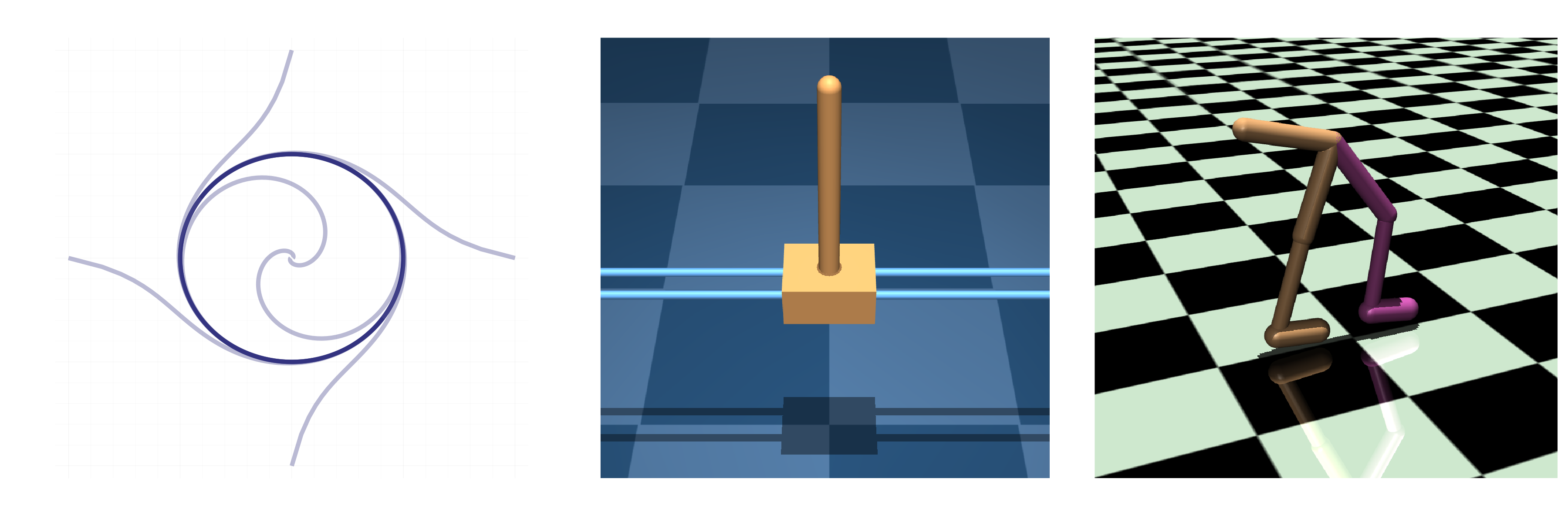
Figure 4: Illustration of some dynamical systems we have used in this work. Left: simple limit cycle represented effectively by the Koopman modes. Middle: DeepMind Control Suite  [Tassa et al., 2018] Cartpole showing stable cycle with spectral radius regularization. Right: OpenAI Gym [Brockman et al., 2016] walker2d showing simpler movement cycle when the Koopman eigenvalues are regularized.

G.1 Cross-entropy method

Throughout, we used CEM for dynamics parameter (policy) selection to approximately solve KSNR. Here, we present the setting of CEM.

First, we prepare some fixed feature (e.g., RFFs) for $\phi$. Then, at each iteration of CEM, we generate many parameters to compute the loss (i.e., the sum of the Koopman spectrum cost and negative cumulative reward) by fitting the transition data generated by each parameter to the feature to estimate its Koopman operator $\mathscr{A}$. In particular, we used the following regularized fitting:

$$\mathscr{A}=YX^{\top}(XX^{\top}+I)^{-1},$$

where $Y:=[\boldsymbol{\phi}_{x_{h_{1}+1,1}},\boldsymbol{\phi}_{x_{h_{2}+1,2}},\ldots,\boldsymbol{\phi}_{x_{h_{n}+1,n}}]$ and $X:=[\boldsymbol{\phi}_{x_{h_{1},1}},\boldsymbol{\phi}_{x_{h_{2},2}},\ldots,\boldsymbol{\phi}_{x_{h_{n},n}}]$. Here,

If the feature spans a Koopman invariant space and the deterministic dynamical systems are considered, and if no regularization (i.e., the identity matrix $I$) is used, any sufficiently rich trajectory data may be used to exactly compute $\mathscr{K}(\Theta)$ for $\Theta$. However, in practice, the estimate depends on transition data although the regularization mitigates this effect. In our simulations, at each iteration, we randomly reset the initial state according to some distribution, and computed loss for each parameter generating trajectory starting from that state.

G.2 On Koopman modes

Suppose that the target Koopman operator $\mathscr{A}^{\star}$ has eigenvalues $\lambda_{i}\in\mathbb{C}$ and eigenfunctions $\xi_{i}:\mathcal{X}\rightarrow\mathbb{C}$ for $i\in\{1,2,\ldots,d_{\phi}\}$, i.e.,

$$\mathscr{A}^{\star}\xi_{i}=\lambda_{i}\xi_{i}.$$

If the observable $\phi$ satisfies

$$\boldsymbol{\phi}_{x}=\sum_{i=1}^{d_{\phi}}\xi_{i}(x)\mathbf{m}^{\star}_{i},$$

for $\mathbf{m}^{\star}_{i}\in\mathbb{C}^{d_{\phi}}$, then $\mathbf{m}^{\star}_{i}$s are called the Koopman modes. The Koopman modes are closely related to the concept isostable; interested readers are referred to [Mauroy et al., 2013] for example.

Now, the spectrum cost $\Lambda(\mathscr{A})=\|\mathbf{m}_{1}-\mathbf{m}_{1}^{\star}\|_{1}$ does not satisfy the Hölder condition (Assumption 4) in general; therefore this cost might not be used for KS-LC³.

G.3 Setups: imitating target behaviors through Koopman operators

The discrete-time dynamics

$$r_{h+1}=r_{h}+v_{r,h}\Delta t,~{}\theta_{h+1}=\theta_{h}+v_{\theta,h}\Delta t$$

is considered and the policy returns $v_{r,h}$ and $v_{\theta,h}$ given $r_{h}$ and $\theta_{h}$. In our simulation, we used $\Delta t=0.05$. Note the ground-truth dynamics

$$\dot{r}=r(1-r^{2}),~{}\dot{\theta}=1,$$

is discretized to

$$r_{h+1}=r_{h}+r_{h}(1-r_{h}^{2})\Delta t,~{}\theta_{h+1}=\theta_{h}+\Delta t.$$

Figure 5 plots the ground-truth trajectories of observations and $x$-$y$ positions.

We trained the target Koopman operator using the ground-truth dynamics with random initializations; the hyperparameters used for training are summarized in Table 1.

Then, we used CEM to select policy so that the spectrum cost is minimized; the hyperparameters are summarized in Table 1.

Table 1: Hyperparameters used for limit cycle generation.

CEM hyperparameter	Value	Training target Koopman operator	Value
samples	$200$	training iteration	$500$
elite size	$20$	RFF bandwidth for $\phi$	$3.0$
iteration	$50$	RFF dimension $d_{\phi}$	$80$
planning horizon	$80$	horizon for each iteration	$80$
policy RFF dimension	$50$
policy RFF bandwidth	$2.0$

We tested two forms of the spectrum cost; $\Lambda_{1}(\mathscr{A})=\|\mathbf{m}-\mathbf{m}^{\star}\|_{1}$ and $\Lambda_{2}(\mathscr{A})=\|\mathscr{A}-\mathscr{A}^{\star}\|^{2}_{\rm HS}$. The resulting trajectories are plotted in Figure 6 and 7, respectively. It is interesting to observe that the top mode imitation successfully converged to the desirable limit cycle while Frobenius norm imitation did not.

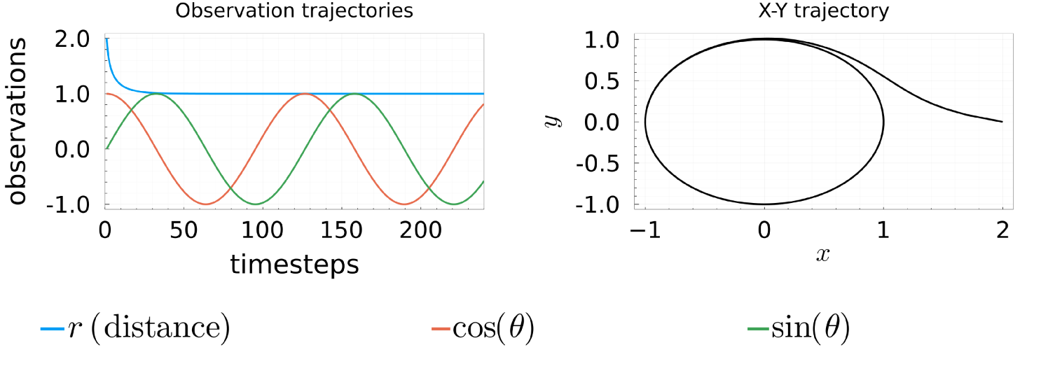
Figure 5: The ground-truth trajectory of the limit cycle $\dot{r}=r(1-r^{2}),~{}\dot{\theta}=1$. Left: observations $r$, $\cos(\theta)$, and $\sin(\theta)$. Right: $x$-$y$ positions.

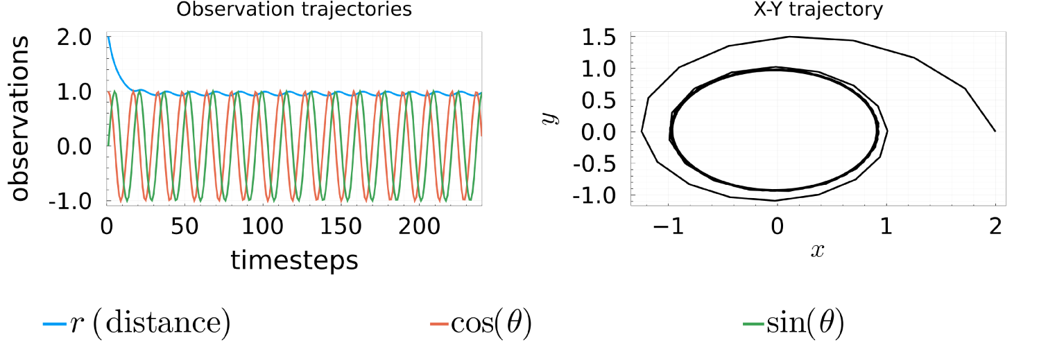
Figure 6: The trajectory generated by RFF policies that minimize $\Lambda(\mathscr{A})=\|\mathbf{m}-\mathbf{m}^{\star}\|_{1}$. Left: observations $r$, $\cos(\theta)$, and $\sin(\theta)$. Right: $x$-$y$ positions.

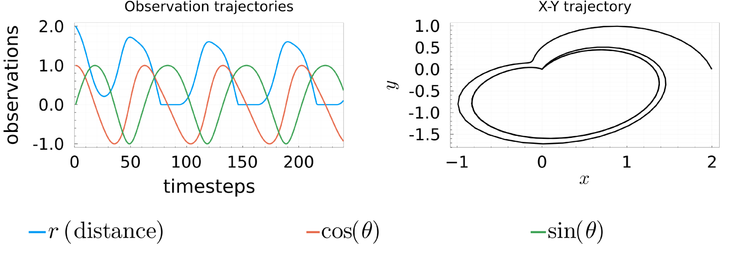
Figure 7: The trajectory generated by RFF policies that minimize $\Lambda(\mathscr{A})=\|\mathscr{A}-\mathscr{A}^{\star}\|^{2}_{\rm HS}$. Left: observations $r$, $\cos(\theta)$, and $\sin(\theta)$. Right: $x$-$y$ positions.

G.4 Setups: Generating stable loops (Cartpole)

We used DeepMind Control Suite Cartpole environment with modifications; specifically, we extended the cart rail to $[-100,100]$ from the original length $[-5,5]$ to deal with divergent behaviors. Also, we used a combination of linear and RFF features; the first elements of the feature are simply the observation (state) vector, and the rest are Gaussian RFFs. That way, we found divergent behaviors were well-captured in terms of spectral radius. The hyperparemeters used for CEM are summarized in Table 2.

Table 2: Hyperparameters used for stable loop generation.

Hyperparameters	Value	Hyperparameters	Value
samples	$200$	elite size	$20$
iteration	$100$	planning horizon	$100$
dimension $d_{\phi}$	$50$	RFF bandwidth for $\phi$	$2.0$
policy RFF dimension	$100$	policy RFF bandwidth	$2.0$

G.5 Generating smooth movements (Walker)

Because of the complexity of the dynamics, we used four random seeds in this simulation, namely, $100$, $200$, $300$, and $400$. We used a combination of linear and RFF features for both $\phi$ and the policy. Note, according to the work [Rajeswaran et al., 2017], linear policy is actually sufficient for some tasks for particular environments. The hyperparemeters used for CEM are summarized in Table 3.

Table 3: Hyperparameters used for Walker.

Hyperparameters	Value	Hyperparameters	Value
samples	$300$	elite size	$20$
iteration	$50$	planning horizon	$300$
dimension of $d_{\phi}$	$200$	RFF bandwidth for $\phi$	$5.0$
policy RFF dimension	$300$	policy RFF bandwidth	$30.0$

The resulting trajectories of Walker are illustrated in Figure 8. The results are rather surprising; because we did not specify the height in reward, the dynamics with only cumulative cost showed rolling behavior (Up figure) to go right faster most of the time. On the other hand, when the spectrum cost was used, the hopping behavior (Down figure) emerged. Indeed this hopping behavior moves only one or two joints most of the time while fixing other joints, which leads to lower (absolute values of) eigenvalues.

The eigenspectrums of the resulting dynamics with/without the spectrum cost are plotted in Figure 9. In fact, it is observed that the dynamics when the spectrum cost was used showed consistently lower (absolute values of) eigenvalues; for the hopping behavior, most of the joint angles converged to some values and stayed there.

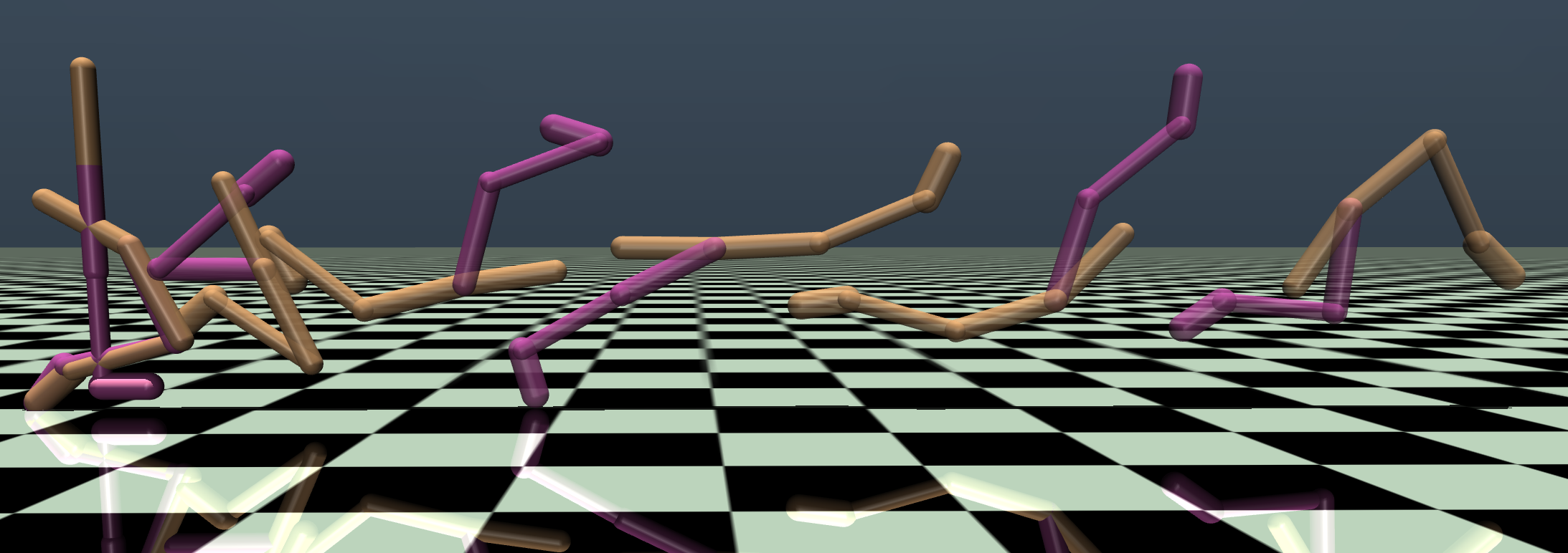
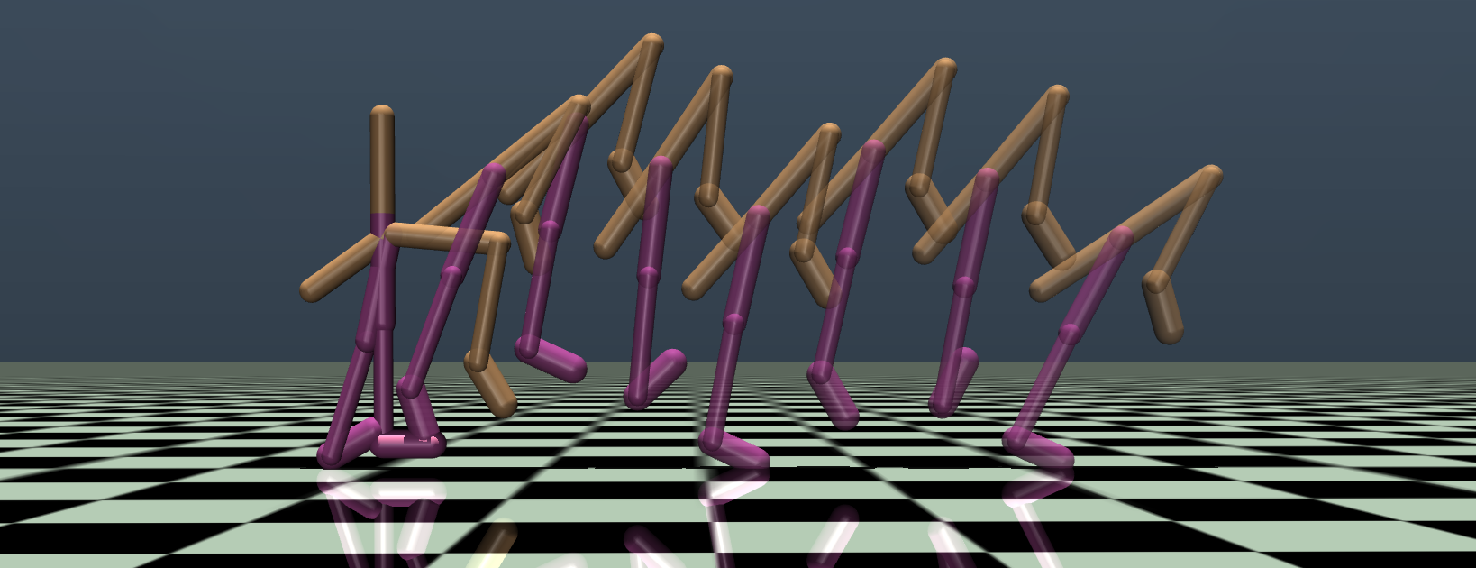
Figure 8: Walker trajectories visualized via Lyceum. Up: when only (single-step) reward $v-0.001\|a\|^{2}_{\mathbb{R}^{6}}$ is used, showing rolling behavior. Down: when the spectrum cost $\Lambda(\mathscr{A})=5\sum_{i=1}^{d_{\phi}}|\lambda_{i}(\mathscr{A})|$ is used together with the reward, showing simple hopping behavior.

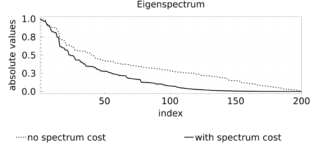
Figure 9: Eigenspectrums showing absolute values of eigenvalues for the dynamics with/without the spectrum cost.

G.6 Setups: Koopman-Spectrum LC³

First, we explain how to reduce the memory size below.

Decomposable kernels case

Assume that we employ decomposable kernel with $B=I$ for simplicity. Also, suppose $\Psi(\Theta)\in\mathbb{R}^{d_{\Psi}\times d_{\phi}}$ is of finite dimension. For such a case, the dimension $d_{\Psi}=d_{\zeta}\cdot d_{\phi}$ where $d_{\zeta}$ is the dimension of $\mathcal{H}^{\prime\prime}$; however, we do not need to store a covariance matrix of size $d_{\phi}^{2}d_{\zeta}\times d_{\phi}^{2}d_{\zeta}$ but only require to update a matrix of size $d_{\phi}d_{\zeta}\times d_{\phi}d_{\zeta}$ which significantly reduces the memory size. Specifically, we consider the model $\boldsymbol{\phi}_{x_{h+1}}={M^{\prime}}(\boldsymbol{\phi}_{x_{h}}\otimes\boldsymbol{\zeta}(\Theta))$; then using $M^{\prime\prime}:={\rm reshape}(M^{\prime},d_{\phi},d_{\zeta},d_{\phi})$, we obtain $\mathscr{K}(\Theta)=[M^{\prime\prime}[:,:,1]\boldsymbol{\zeta}(\Theta),\ldots,M^{\prime\prime}[:,:,d_{\phi}]\boldsymbol{\zeta}(\Theta)]$. Here, $\boldsymbol{\zeta}$ is the realization of $\zeta(\Theta)$ over some basis. Now, we note that the dimension of $\boldsymbol{\phi}_{x_{h}}\otimes\boldsymbol{\zeta}(\Theta)$ is $d_{\zeta}\cdot d_{\phi}$. Our practical (Thompson sampling version) algorithm is thus given by Algorithm 2.

1:Parameter set $\Pi$; prior parameter $\lambda$; covariance scale $\iota\in\mathbb{R}_{\geq 0}$.

2:Prior distribution over $M^{\prime}$ is given by $\Sigma_{M^{\prime}}^{0}:=\lambda I$

3:for $t=0\dots T-1$ do

4:     Adversary chooses $X^{t}_{0}$.

5:     Sample $\hat{M^{\prime}}^{t}$ from $\mathcal{N}\left(\overline{M^{\prime}}^{t},\Sigma_{M^{\prime}}^{t}\right)$

6:     Solve $\Theta^{t}=\operatorname*{arg\,min}_{\Theta\in\Pi}\Lambda[\hat{\mathscr{K}}^{t}(\Theta)]+J^{\Theta}\left(X^{t}_{0};\hat{M^{\prime}}^{t};c^{t}\right)$ (e.g., using CEM)

7:     Under the dynamics $\mathcal{F}^{\Theta^{t}}$, sample transition data $\tau^{t}:=\{\tau^{t}_{n}\}_{n=0}^{N^{t}-1}$, where $\tau^{t}_{n}:=\{x^{t}_{h,n}\}_{h=0}^{H^{t}_{n}}$

8:     Update $\Sigma_{M^{\prime}}^{t}$

9:end for

Algorithm 2 Practical Algorithm for KS-LC³

In the algorithm, we used $\hat{\mathscr{K}}^{t}(\Theta)=[\hat{M^{\prime\prime}}^{t}[:,:,1]\boldsymbol{\zeta}(\Theta),\ldots,\hat{M^{\prime\prime}}^{t}[:,:,d_{\phi}]\boldsymbol{\zeta}(\Theta)]$, where $\hat{M^{\prime\prime}}^{t}:={\rm reshape}(\hat{M^{\prime}}^{t},d_{\phi},d_{\zeta},d_{\phi})$.

Pretraining policies

For training three policies, we used Model Predictive Path Integral Control (MPPI) [Williams et al., 2017] with the rewards $(p+0.3)^{2}$, $(p-0.3)^{2}$, $(v+1.5)^{2}$, and $(v-1.5)^{2}$, where $p$ is the cart position and $v$ is the cart velocity. Also, for all of the cases, the penalty $-100$ is added when $\cos(\theta)<0$, where $\theta$ is the pole angle, which aims at preventing the pole from falling down.

Because we need to have one more state dimension to specify which reward to generate, we used the analytical model of cartpole specified in OpenAI Gym.

Starting from random initial state, we first use MPPI to move to $p=-0.3$, then from there move to $p=0.3$; and we learn an RFF policy for this movement along with the Koopman operator. Then, we randomly initialized the state to accelerate to $v=-1.5$, followed by a random initialization again to accelerate to $v=1.5$; we then learned two policies for those two movements. We used the planning horizons of $100$ for every movement except for the movement going to $p=0.3$ where we used $120$ because it is following the previous movement. We repeated this for $20$ iterations.

The parameter space $\Pi$ is a space of linear combinations of those three policies. We summarized the hyperparemeters used for MPPI/pretraining in Table 4.

Table 4: Hyperparameters of MPPI and pretraining.

MPPI hyperparameters	Value	Pretraining hyperparameters	Value
variance of controls	$0.4^{2}$	iteration	$20$
temperature parameter	$0.1$	policy RFF dimension	$2000$
planning horizon	$100/120$	policy RFF bandwidth	$1.5$
number of planning samples	$524$	dimension of $d_{\phi}$	$60$
		RFF bandwidth for $\phi$	$1.5$

Learning

For learning, we used four random seeds, namely, $100$, $200$, $300$, and $400$. The estimated spectrum cost curve represents the cost $\Lambda[\hat{\mathscr{K}}^{t}(\Theta^{t})]$. The hyperparameters used for CEM and KS-LC³ are summarized in Table 5. We note that for KS-LC³ we added additional cost on the policy parameter exceeding its $\ell_{\infty}$ norm above $2.0$.

Table 5: Hyperparameters used for CEM/KS-LC³.

Hyperparameters for CEM	Value	Hyperparameters for KS-LC3	Value
samples	$200$	dimension of $d_{\zeta}$	$50$
elite size	$20$	RFF bandwidth for $\zeta$	$5.0$
planning horizon	$500$	prior parameter $\lambda$	$1.0$
iteration	$50$	covariance scale $\iota$	$0.0001$

References

- Abraham and Murphey [2019] I. Abraham and T. D. Murphey. Active learning of dynamics for data-driven control using Koopman operators. IEEE Trans. Robotics, 35(5):1071–1083, 2019.
- Andry et al. [1983] AN Andry, EY Shapiro, and JC Chung. Eigenstructure assignment for linear systems. IEEE transactions on aerospace and electronic systems, (5):711–729, 1983.
- Arnold [1995] L. Arnold. Random dynamical systems. In Dynamical systems, pages 1–43. Springer, 1995.
- Bezanson et al. [2017] J. Bezanson, A. Edelman, S. Karpinski, and V. B. Shah. Julia: A fresh approach to numerical computing. SIAM review, 59(1):65–98, 2017.
- Brault et al. [2016] R. Brault, M. Heinonen, and F. Buc. Random fourier features for operator-valued kernels. In Proc. ACML, pages 110–125, 2016.
- Brockman et al. [2016] G. Brockman, V. Cheung, L. Pettersson, J. Schneider, J. Schulman, J. Tang, and W. Zaremba. OpenAi Gym. arXiv preprint arXiv:1606.01540, 2016.
- Črnjarić-Žic et al. [2019] N. Črnjarić-Žic, S. Maćešić, and I. Mezić. Koopman operator spectrum for random dynamical systems. Journal of Nonlinear Science, pages 1–50, 2019.
- Curi et al. [2020] S. Curi, F. Berkenkamp, and A. Krause. Efficient model-based reinforcement learning through optimistic policy search and planning. arXiv preprint arXiv:2006.08684, 2020.
- Eysenbach et al. [2018] B. Eysenbach, A. Gupta, J. Ibarz, and S. Levine. Diversity is all you need: Learning skills without a reward function. arXiv preprint arXiv:1802.06070, 2018.
- Grafakos [2008] L. Grafakos. Classical Fourier analysis, volume 2. Springer, 2008.
- Hemati and Yao [2017] M. Hemati and H. Yao. Dynamic mode shaping for fluid flow control: New strategies for transient growth suppression. In 8th AIAA Theoretical Fluid Mechanics Conference, page 3160, 2017.
- Ibarz et al. [2021] J. Ibarz, J. Tan, C. Finn, M. Kalakrishnan, P. Pastor, and S. Levine. How to train your robot with deep reinforcement learning: lessons we have learned. International Journal of Robotics Research, 40(4-5):698–721, 2021.
- Ishikawa et al. [2018] I. Ishikawa, K. Fujii, M. Ikeda, Y. Hashimoto, and Y. Kawahara. Metric on nonlinear dynamical systems with Perron-Frobenius operators. In Proc. NeurIPS, pages 2856–2866. 2018.
- Iwata and Kawahara [2020] T. Iwata and Y. Kawahara. Neural dynamic mode decomposition for end-to-end modeling of nonlinear dynamics. arXiv:2012.06191, 2020.
- Jiang et al. [2017] N. Jiang, A. Krishnamurthy, A. Agarwal, J. Langford, and R. E. Schapire. Contextual decision processes with low Bellman rank are PAC-learnable. In Proc. ICML, pages 1704–1713, 2017.
- Kadri et al. [2016] H. Kadri, E. Duflos, P. Preux, S. Canu, A. Rakotomamonjy, and J. Audiffren. Operator-valued kernels for learning from functional response data. Journal of Machine Learning Research, 17(20):1–54, 2016.
- Kaiser et al. [2021] E. Kaiser, J. N. Kutz, and S. Brunton. Data-driven discovery of Koopman eigenfunctions for control. Machine Learning: Science and Technology, 2021.
- Kakade et al. [2020] S. Kakade, A. Krishnamurthy, K. Lowrey, M. Ohnishi, and W. Sun. Information theoretic regret bounds for online nonlinear control. Proc. NeurIPS, 2020.
- Kawahara [2016] Y. Kawahara. Dynamic mode decomposition with reproducing kernels for Koopman spectral analysis. Proc. NeurIPS, 29:911–919, 2016.
- Kober et al. [2013] J. Kober, J. A. Bagnell, and J. Peters. Reinforcement learning in robotics: A survey. International Journal of Robotics Research, 32(11):1238–1274, 2013.
- Kobilarov [2012] M. Kobilarov. Cross-entropy motion planning. The International Journal of Robotics Research, 31(7):855–871, 2012.
- Koopman [1931] B. O. Koopman. Hamiltonian systems and transformation in Hilbert space. Proc. National Academy of Sciences of the United States of America, 17(5):315, 1931.
- Korda and Mezić [2018] M. Korda and I. Mezić. Linear predictors for nonlinear dynamical systems: Koopman operator meets model predictive control. Automatica, 93:149–160, 2018.
- Korda and Mezić [2020] M. Korda and I. Mezić. Optimal construction of Koopman eigenfunctions for prediction and control. IEEE Trans. Automatic Control, 65(12):5114–5129, 2020.
- Kutz et al. [2016] J. N. Kutz, S. L. Brunton, B. W. Brunton, and J. L. Proctor. Dynamic mode decomposition: Data-driven modeling of complex systems. SIAM, 2016.
- Li et al. [2019] Y. Li, H. He, J. Wu, D. Katabi, and A. Torralba. Learning compositional Koopman operators for model-based control. arXiv preprint arXiv:1910.08264, 2019.
- Manek and Kolter [2019] G. Manek and J Zico Kolter. Learning stable deep dynamics models. Proc. NeurIPS, 2019.
- Mania et al. [2020] H. Mania, M. I. Jordan, and B. Recht. Active learning for nonlinear system identification with guarantees. arXiv preprint arXiv:2006.10277, 2020.
- Mauroy and Mezić [2016] A. Mauroy and I. Mezić. Global stability analysis using the eigenfunctions of the Koopman operator. IEEE Trans. Automatic Control, 61(11):3356–3369, 2016.
- Mauroy et al. [2013] A. Mauroy, I. Mezić, and J. Moehlis. Isostables, isochrons, and Koopman spectrum for the action–angle representation of stable fixed point dynamics. Physica D: Nonlinear Phenomena, 261:19–30, 2013.
- Mauroy et al. [2020] A. Mauroy, Y. Susuki, and I. Mezić. The Koopman operator in systems and control. Springer, 2020.
- Mezić [2005] I. Mezić. Spectral properties of dynamical systems, model reduction and decompositions. Nonlinear Dynamics, 41:309–325, 2005.
- Mnih et al. [2013] V. Mnih, K. Kavukcuoglu, D. Silver, A. Graves, I. Antonoglou, D. Wierstra, and M. Riedmiller. Playing Atari with deep reinforcement learning. arXiv preprint arXiv:1312.5602, 2013.
- Mnih et al. [2015] V. Mnih, K. Kavukcuoglu, D. Silver, A. A. Rusu, J. Veness, M. G. Bellemare, A. Graves, M. Riedmiller, A. K. Fidjeland, G. Ostrovski, et al. Human-level control through deep reinforcement learning. Nature, 518(7540):529–533, 2015.
- Nakao [2017] H. Nakao. Phase reduction approach to synchronization of nonlinear oscillators. Contemporary Physics, 57(2):188–214, 2017.
- Ng and Russell [2000] A. Y. Ng and S. J. Russell. Algorithms for inverse reinforcement learning. In Proc. ICML, volume 1, 2000.
- Pintelon and Schoukens [2012] R. Pintelon and J. Schoukens. System identification: a frequency domain approach. John Wiley & Sons, 2012.
- Rahimi and Recht [2007] A. Rahimi and B. Recht. Random features for large-scale kernel machines. Proc. NeurIPS, 2007.
- Rajeswaran et al. [2017] A. Rajeswaran, K. Lowrey, E. Todorov, and S. Kakade. Towards generalization and simplicity in continuous control. Proc. NeurIPS, 2017.
- Sabanovic and Ohnishi [2011] A. Sabanovic and K. Ohnishi. Motion control systems. John Wiley & Sons, 2011.
- Simchowitz and Foster [2020] M. Simchowitz and D. Foster. Naive exploration is optimal for online LQR. In Proc. ICML, pages 8937–8948, 2020.
- Song [2002] Y. Song. A note on the variation of the spectrum of an arbitrary matrix. Linear algebra and its applications, 342(1-3):41–46, 2002.
- Strogatz [2018] S. H. Strogatz. Nonlinear dynamics and chaos with student solutions manual: With applications to physics, biology, chemistry, and engineering. CRC press, 2018.
- Summers et al. [2020] C. Summers, K. Lowrey, A. Rajeswaran, S. Srinivasa, and E. Todorov. Lyceum: An efficient and scalable ecosystem for robot learning. In Learning for Dynamics and Control, pages 793–803. PMLR, 2020.
- Sun et al. [2019] W. Sun, N. Jiang, A. Krishnamurthy, A. Agarwal, and J. Langford. Model-based RL in contextual decision processes: PAC bounds and exponential improvements over model-free approaches. In Proc. COLT, pages 2898–2933, 2019.
- Takeishi and Kawahara [2021] N. Takeishi and Y. Kawahara. Learning dynamics models with stable invariant sets. In Proc. AAAI, 2021.
- Tassa et al. [2018] Y. Tassa, Y. Doron, A. Muldal, T. Erez, Y. Li, D. L. Casas, D. Budden, A. Abdolmaleki, J. Merel, A. Lefrancq, et al. DeepMind Control Suite. arXiv preprint arXiv:1801.00690, 2018.
- Todorov et al. [2012] E. Todorov, T. Erez, and Y. Tassa. MuJoCo: A physics engine for model-based control. In IEEE/RSJ IROS, pages 5026–5033, 2012.
- Williams et al. [2017] G. Williams, A. Aldrich, and E. A. Theodorou. Model predictive path integral control: From theory to parallel computation. Journal of Guidance, Control, and Dynamics, 40(2):344–357, 2017.
- Winfree [2001] A. T. Winfree. The Geometry of Biological Time. Springer, 2001.