Abstract

An efficient algorithm is developed for compactly weaving all the Lorentz covariant three-point vertices in relation to the decay of a massive particle $X$ of mass $m_{X}$ and spin $J$ into two particles $M_{1,2}$ with equal mass $m$ and spin $s$. The closely-related equivalence between the helicity formalism and the covariant formulation is utilized so as to identify the basic building blocks for constructing the covariant three-point vertex corresponding to each helicity combination explicitly. The massless case with $m=0$ is worked out straightforwardly and the (anti)symmetrization of the three-point vertex required by spin statistics of identical particles is made systematically. It is shown that the off-shell electromagnetic photon coupling to the states $M_{1}$ and $M_{2}$ can be accommodated in this framework. The power of the algorithm is demonstrated with a few typical examples with specific $J$ and $s$ values.

1 Introduction

The Standard Model (SM) [1, 2, 3, 4] of particle physics has been firmly established by the discovery of the spin-0 resonance of about 125  GeV mass at the Large Hadron Collider (LHC) at CERN [5, 6]. However, even though a lot of high-energy experiments have searched for new phenomena beyond the SM (BSM) and they have tested the SM with great precision for decades, none of any BSM particles and phenomena has been observed so far at the TeV scale (see Ref. [7] for a comprehensive summary of hypothetical particles and concepts). In this present situation considered to be unnatural, one meaningful strategy that can be taken in new physics searches is to keep our theoretical studies as model-independent as possible and to search for new particles with even more exotic characteristics including spins higher than unity.

Recently, the theory and phenomenology of high-spin particles [8, 9, 10, 11, 12, 13, 14, 15, 16, 17, 18] have drawn considerable interest. Various high-spin particles, although composite, exist in hadron physics (see Ref. [7] for several high-spin hadrons) so that the solid theoretical calculations of all the rates and distributions involving such high-spin states are required for correctly interpreting all the relevant experimental results [8, 9, 10]. A popular spin-3/2 particle is the gravitino appearing as the supersymmetric partner of the massless spin-2 graviton in supergravity [19, 20, 21, 22, 23]. The discovery of gravitational waves [24, 25, 26] strongly indicates the existence of massless spin-2 gravitons at the quantum level. The massive spin-2 particles as the Kaluza-Klein (KK) excitations of the massless graviton have been studied in the context of extra dimensional scenarios [27, 28, 29]. In addition, whether the dark matter (DM) of the Universe is formed with high-spin particles has been addressed in various recent works [11, 12, 13, 14, 15, 16, 17]. The relic density of the high-spin DM particles and their low-energy interactions with the SM particles have to be evaluated precisely for checking the plausibility of their indirect and direct observations. For studying all of these theoretical and phenomenological aspects, it is crucial to systematically investigate all the allowed effective interactions of high-spin particles as well as the SM spin-$0$, $1/2$ and $1$ particles in a model-independent way.

In the present work, we focus on developing an efficient algorithm for compactly weaving all the three-point vertices consistent with Lorentz invariance and locality. Specifically, we consider the decay of a massive particle of mass $m_{X}$ and spin $J$ into two massive particles, $M_{1}$ and $M_{2}$, of equal mass $m$ and spin $s$. This study is a natural extension of the previous work [30] having dealt with the massless ($m=0$) case with the identical particle (IP) condition imposed, and an intermediate bridge to the general case where all the three particles have different masses and spins. We adopt the conventional description of the integer and half-integer wave tensors [31, 32, 33, 34, 35, 36, 37] and we effectively utilize the closely-related equivalence between the helicity formalism in the Jacob-Wick (JW) convention [38, 39] and the standard covariant formulation. Their one-to-one correspondence enables us to identify every basic building block for constructing the covariant three-point vertex corresponding to each helicity combination explicitly. we show that the massless ($m=0$) case treated previously [30] can be worked out straightforwardly and the (anti)symmetrization of the vertex required by spin statistics of identical particles [41] can be made systematically. The extension of the algorithm to the case where all the three particles have different masses and spins is briefly touched upon.

This paper is organized as follows. In Section 2, we discuss the key aspects of the two-body decay process $X\to M_{1}M_{2}$ in the helicity formalism which allows us to treat any massive and massless particles on an equal footing. Section 3 is devoted to explicitly deriving and characterizing the integer and half-integer spin-$s$ wave tensors and the spin-$J$ wave tensor based on the conventional combination of spin-1 wave vectors and spin-1/2 spinors. In particular, the wave vectors and spinors in the $X$ rest frame ($X$RF) are presented explicitly in the JW convention. Utilizing the close inter-relationship between the helicity formalism and the covariant formulation we derive all the covariant basic and composite three-point operators both in the bosonic and fermionic case in Section 4. In Section 5, the composite operators are shown to enable us to explicitly write down all the helicity-specific three-point vertices through which the covariant three-point vertex for any spin $J$ and spin $s$ can be weaved efficiently both in the massive and massless cases. In addition, we show that the relation valid in the case with two identical particles in the final state is systematically and straightforwardly derived and that the off-shell electromagnetic photon coupling to the states $M_{1}$ and $M_{2}$ can be accommodated in this framework. In order to demonstrate the power of the developed algorithm for constructing the covariant three-point vertices, we work out in detail several examples with specific $J$ and $s$ values, which are expected to be useful for various phenomenological investigations, in Section 6. Finally, we summarize our findings and conclude the present work by mentioning a few topics under study in Section 7.

2 Characterization in the helicity formalism

The helicity formalism [38, 39] allows us to efficiently describe the two-body decay of a spin-$J$ particle $X$ of mass $m_{X}$ into two massive particles, $M_{1}$ and $M_{2}$, with equal mass $m$ and spin $s$. For the sake of a transparent and straightforward analytic analysis, we describe the two-body decay $X\to M_{1}M_{2}$ in the $X$RF

$$X(p,\sigma)\ \ \rightarrow\ \ M_{1}(k_{1},\lambda_{1})\,+\,M_{2}(k_{2},\lambda_{2})\,,$$ (2.1)

in terms of the momenta, $\{p,k_{1},k_{2}\}$, and helicities, $\{\sigma,\lambda_{1},\lambda_{2}\}$, of the particles, as depicted in Figure 1.

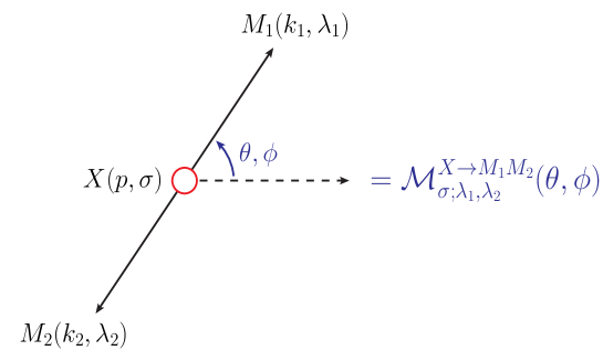
Figure 1: Kinematic configuration for the helicity amplitude ${\cal M}^{X\to M_{1}M_{2}}_{\sigma;\,\lambda_{1},\lambda_{2}}(\theta,\phi)$ of the two-body decay $X\to M_{1}M_{2}$ of a massive particle $X$ into two massive particles, $M_{1}$ and $M_{2}$, in the $X$RF. The notations, $\{p,k_{1,2}\}$ and $\{\sigma,\lambda_{1,2}\}$, are the momenta and helicities of the decaying particle $X$ and two particles, $M_{1}$ and $M_{2}$, respectively. The polar and azimuthal angles, $\theta$ and $\phi$, are defined with respect to an appropriately chosen coordinate system.

The helicity amplitude of the decay $X\to M_{1}M_{2}$ is decomposed in terms of the polar and azimuthal angles, $\theta$ and $\phi$, defining the momentum direction of the particle $M_{1}$ in a fixed coordinate system as

$${\cal M}^{X\to MM}_{\sigma;\lambda_{1},\lambda_{2}}(\theta,\phi)\,\,=\,\,{\cal C}^{J}_{\lambda_{1},\lambda_{2}}\,\,d^{J}_{\sigma,\,\lambda_{1}-\lambda_{2}}(\theta)\,e^{i(\sigma-\lambda_{1}+\lambda_{2})\phi}\quad\ \ \mbox{with}\quad\ \ |\lambda_{1}-\lambda_{2}|\leq J\,,$$ (2.2)

with the constraint $|\lambda_{1}-\lambda_{2}|\leq J$ in the JW convention [38, 39] (see Figure 1 for the kinematic configuration). Here, the helicity $\sigma$ of the spin-$J$ massive particle $X$ takes one of $2J+1$ values between $-J$ and $J$. In contrast, each of the helicities, $\lambda_{1,2}$, can take one of $2s+1$ values between $-s$ and $s$ in the massive ($m\neq 0$) case but they take just two values of $\pm s$ in the massless ($m=0$) case, as only the maximal-magnitude helicity values identical to the spin in magnitude are allowed physically for a massless particle of any spin. The reduced helicity amplitudes ${\cal C}^{J}_{\lambda_{1},\lambda_{2}}$ in Eq. (2.2) do not depend on the $X$ helicity $\sigma$ due to rotational invariance and the polar-angle dependence is fully encoded in the Wigner $d$ function $d^{J}_{\sigma,\lambda_{1}-\lambda_{1}}(\theta)$ given in the convention of Rose [42].

If two particles, $M_{1}$ and $M_{2}$, are identical, the Bose or Fermi symmetry in the integer or half-integer case leads to the IP relation for the reduced helicity amplitudes:

$${\cal C}^{J}_{\lambda_{1},\lambda_{2}}\,\,=\,\,(-1)^{J}\,\,{\cal C}_{\lambda_{2},\lambda_{1}}\ \ \ \ \mbox{with}\ \ \ \ |\lambda_{1}-\lambda_{2}|\leq J\,,$$ (2.3)

due to the (anti)-symmetrization of the two identical final-state particles.

First, in the massive ($m\neq 0$) case, the number $n\,[J,s]$ of independent reduced helicity amplitudes for specific $J$ and $s$ is

$$n\,[J,s]\,=\,\left\{\begin{array}[]{ll}(2s+1)^{2}&\ \ \mbox{for}\ \ J\geq 2s\,,\\[8.53581pt] 2s+1+(4s+1)J-J^{2}&\ \ \mbox{for}\ \ J<2s\,.\end{array}\right.$$ (2.6)

For example, we have $n\,[J,0]=1$, $n\,[1,1]=7$ and $n\,[2,1]=9$. On the other hand, the number of independent terms in the IP case reduces to

$$n\,[J,s]_{\rm IP}\,=\,\left\{\begin{array}[]{ll}\frac{1}{2}(2s+1)\left[1+(-1)^{J}\right]+s(2s+1)&\ \ \mbox{for}\ \ J\geq 2s\,,\\[11.38109pt] \frac{1}{2}(2s+1)\left[1+(-1)^{J}\right]+\frac{1}{2}\left[(4s+1)J-J^{2}\right]&\ \ \mbox{for}\ \ J<2s\,,\end{array}\right.$$ (2.9)

which depends crucially on whether the $X$ spin $J$ is even or odd. For example, $n\,[J,0]_{\rm IP}=[1+(-1)^{J}]/2$, $n\,[1,1]_{\rm IP}=2$ and $n\,[2,1]_{\rm IP}=6$. Therefore, any particle with an odd spin $J$ cannot decay into two identical spinless particles.

In contrast, in the massless ($m=0$) case, the number $n\,[J,s]$ of independent reduced helicity amplitudes is reduced to

$$n\,[J,s]\,=\,\left\{\begin{array}[]{ll}4&\ \ \mbox{for}\ \ J\geq 2s\\[8.53581pt] 2&\ \ \mbox{for}\ \ J<2s\end{array}\right.\ \ \mbox{for}\ \ s>0\quad\mbox{and}\quad n\,[J,0]\,=\,1\,.$$ (2.12)

The number of independent terms in the case with $s=0$ is one, irrespective of the $X$ spin $J$. On the other hand the number of independent terms in the IP case is further reduced to

$$n\,[J,s]_{\rm IP}\,=\,\left\{\begin{array}[]{ll}2+(-1)^{J}&\ \ \mbox{for}\ \ J\geq 2s\\[8.53581pt] 1+(-1)^{J}&\ \ \mbox{for}\ \ J<2s\end{array}\right.\ \ \mbox{for}\ \ s>0\quad\mbox{and}\quad n\,[J,0]\,=\,\frac{1}{2}\,[1+(-1)^{J}]\,,$$ (2.15)

due to the Bose or Fermi symmetry. One immediate consequence is that any odd-$J$ particle cannot decay into two identical massless particles of spin $s$ larger than $J/2$ [30]. One well-known example is that the decay of a spin-1 particle into two identical spin-1 massless particles like two photons [43, 44].

3 Spin-$J$ and spin-$s$ wave tensors

Generically, the decay amplitude of one spin-$J$ particle $X$ of mass $m_{X}$ into two particles, $M_{1}$ and $M_{2}$, of equal mass $m$ and spin $s$, can be written in terms of the three-point vertex tensor $\Gamma$ (see Figure 2 for its diagrammatic description)

$${\cal M}^{X\to M_{1}M_{2}}_{\sigma;\lambda_{1},\lambda_{2}} = \bar{u}_{1}^{\alpha_{1}\cdots\alpha_{n}}(k_{1},\lambda_{1})\,\,\Gamma^{\mu_{1}\cdots\mu_{J}}_{\alpha_{1}\cdots\alpha_{n},\beta_{1}\cdots\beta_{n}}(p,k)\,\,v_{2}^{\beta_{1}\cdots\beta_{n}}(k_{2},\lambda_{2})\,\,\epsilon_{\mu_{1}\cdots\mu_{J}}(p,\sigma)\,,$$ (3.1)

with the non-negative integer $n=s$ or $n=s-1/2$ in the integer or half-integer spin $s$ case, respectively. $p$ and $\sigma$ are the momentum and helicity of the particle $X$, and $k_{1,2}$ and $\lambda_{1,2}$ are the momenta and helicities of two particles, $M_{1}$ and $M_{2}$, respectively. Here, $p=k_{1}+k_{2}$ and $k=k_{1}-k_{2}$ are symmetric and anti-symmetric under the interchange of two momenta, $k_{1}$ and $k_{2}$.

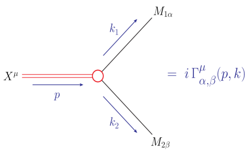
Figure 2: Feynman rules $\Gamma^{\mu}_{\alpha,\beta}(p,k)$ for the general $XM_{1}M_{2}$ three-point vertex of a spin-$J$ particle $X$ of mass $m_{X}$ and two massive particles $M_{1}$ and $M_{2}$ of equal mass $m$ and spin $s$. The indices, $\mu$, $\alpha$ and $\beta$, stand for the sequences of $\mu=\mu_{1}\cdots\mu_{{}_{J}}$,  $\alpha_{1}\cdots\alpha_{n}$ and $\beta_{1}\cdots\beta_{n}$ collectively with the non-negative integer $n=s$ or $n=s-1/2$ in the integer or half-integer spin $s$ case. The symmetric and anti-symmetric momentum combinations, $p=k_{1}+k_{2}$ and $k=k_{1}-k_{2}$, are introduced for systematic classifications of the three-point vertex tensor.

If the spin $s$ is an integer, then the bosonic wave tensors $\bar{u}_{1}^{\alpha_{1}\cdots\alpha_{s}}(k_{1},\lambda_{1})$ and $v_{2}^{\beta_{1}\cdots\beta_{s}}(k_{2},\lambda_{2})$ for the particles with non-zero mass $m$ are given by

$$\bar{u}_{1}^{\alpha_{1}\cdots\alpha_{s}}(k_{1},\lambda_{1})\, = \,\epsilon_{1}^{*\alpha_{1}\cdots\alpha_{s}}(k_{1},\lambda_{1})\,,$$ (3.2)

$$v_{2}^{\beta_{1}\cdots\beta_{s}}(k_{2},\lambda_{2})\, = \,\epsilon_{2}^{*\beta_{1}\cdots\beta_{s}}(k_{2},\lambda_{2})\,,$$ (3.3)

each of which is explicitly given by [31, 32, 33, 34, 35, 36, 37]

$$\epsilon^{*\alpha_{1}\cdots\alpha_{s}}_{1}(k_{1},\lambda_{1}) = \sqrt{\frac{2^{s}\,(s+\lambda_{1})!\,(s-\lambda_{1})!}{(2s)!}}\,\sum^{1}_{\{\tau\}=-1}\,\delta_{\tau_{1}+\cdots+\tau_{s},\,\lambda_{1}}\,\prod_{i=1}^{s}\,\frac{\epsilon_{1}^{*\alpha_{i}}(k_{1},\tau_{i})}{\sqrt{2}^{|\tau_{i}|}}\,,$$ (3.4)

$$\epsilon^{*\beta_{1}\cdots\beta_{s}}_{2}(k_{2},\lambda_{2}) = \sqrt{\frac{2^{s}\,(s+\lambda_{2})!\,(s-\lambda_{2})!}{(2s)!}}\,\sum^{1}_{\{\tau\}=-1}\,\delta_{\tau_{1}+\cdots+\tau_{s},\,\lambda_{2}}\,\prod_{i=1}^{s}\,\frac{\epsilon_{2}^{*\beta_{i}}(k_{2},\tau_{i})}{\sqrt{2}^{|\tau_{i}|}}\,,$$ (3.5)

with the convention $\{\tau\}=\tau_{1},\cdots,\tau_{s}$ as a linear combination of products of $s$ polarization vectors with appropriate Clebsch-Gordon coefficients. We note that the bosonic wave tensors are totally symmetric, traceless and divergence-free

$$\varepsilon_{\mu\nu\alpha_{i}\alpha_{j}}\,\epsilon_{a}^{\alpha_{1}\cdots\alpha_{i}\cdots\alpha_{j}\cdots\alpha_{s}}(k_{a},\lambda_{a}) = 0\,,$$ (3.6)

$$g_{\alpha_{i}\alpha_{j}}\,\epsilon_{a}^{\alpha_{1}\cdots\alpha_{i}\cdots\alpha_{j}\cdots\alpha_{s}}(k_{a},\lambda_{a}) = 0\,,$$ (3.7)

$$k_{\alpha_{i}}\,\epsilon_{a}^{\alpha_{1}\cdots\alpha_{i}\cdots\alpha_{s}}(k_{a},\lambda_{a}) = 0\,,$$ (3.8)

with $a=1$ and $2$, and both of them satisfy the same on-shell wave equation $(k^{2}_{1,2}-m^{2})\,\epsilon_{1,2}^{\alpha_{1}\cdots\alpha_{s}}(k_{1,2},\lambda_{1,2})=0$ for any helicity value of $\lambda_{1,2}$ taking an integer between $-s$ and $s$. In contrast, if $m=0$, the wave tensors with two allowed helicities $\pm s$ are given simply by a direct product of $s$ spin-1 polarization vectors, each of which carries the same helicity of $\pm 1$, as

$$\bar{u}_{1}(k_{1},\pm s)\,=\,\epsilon_{1}^{*\alpha_{1}\cdots\alpha_{s}}(k_{1},\pm s)\,=\,\epsilon_{1}^{*\alpha_{1}}(k_{1},\pm 1)\cdots\epsilon_{1}^{*\alpha_{s}}(k_{1},\pm 1)\,,$$ (3.9)

$$v_{2}(k_{2},\pm s)\,\,=\,\epsilon_{2}^{*\beta_{1}\cdots\beta_{s}}(k_{2},\pm s)\,\,=\,\epsilon_{2}^{*\beta_{1}}(k_{2},\pm 1)\cdots\epsilon_{2}^{*\beta_{s}}(k_{2},\pm 1)\,,$$ (3.10)

which are totally symmetric, traceless and divergence-free in the four-vector indices, $\alpha=\alpha_{1}\cdots\alpha_{s}$ and $\beta=\beta_{1}\cdots\beta_{s}$, as well.

On the other hand, for a half-integer $s=n+1/2$ with a non-negative integer $n$, the fermionic wave tensors for the particles with non-zero mass are given by [31, 32, 33, 34, 36, 37]

$$\mbox{ }\hskip-36.98866pt\bar{u}^{\alpha_{1}\cdots\alpha_{n}}_{1}(k_{1},\lambda_{1})=\sum_{\tau=\pm\frac{1}{2}}\,\sqrt{\frac{s+2\tau\lambda_{1}}{2s}}\,\,\epsilon^{*\alpha_{1}\cdots\alpha_{n}}_{1}(k_{1},\lambda_{1}-\tau)\,\bar{u}(k_{1},\tau)\,,$$ (3.11)

$$\mbox{ }\hskip-36.98866ptv^{\alpha_{1}\cdots\alpha_{n}}_{2}(k_{2},\lambda_{2})=\sum_{\tau=\pm\frac{1}{2}}\,\sqrt{\frac{s+2\tau\lambda_{2}}{2s}}\,\,\epsilon^{*\alpha_{1}\cdots\alpha_{n}}_{2}(k_{2},\lambda_{2}-\tau)\,v_{2}(k_{2},\tau)\,,$$ (3.12)

where $\bar{u}_{1}(k_{1},\mbox{\small$\pm\frac{1}{2}$})=u^{\dagger}_{1}(k_{1},\mbox{\small$\pm\frac{1}{2}$})\gamma^{0}$ with the spin-1/2 particle spinor $u_{1}(k_{1},\mbox{\small$\pm\frac{1}{2}$})$, and $v_{2}(k_{2},\mbox{\small$\pm\frac{1}{2}$})$ is the spin-1/2 anti-particle spinor. The spin-1/2 spinors satisfy their own on-shell equations, $(\not\!\!{k}_{1}-m)u_{1}(k_{1},\mbox{\small$\pm\frac{1}{2}$})=0$ and $(\not\!\!{k}_{2}+m)v_{2}(k_{2},\mbox{\small$\pm\frac{1}{2}$})=0$. In contrast, if $m=0$, the wave tensors with two allowed helicities $\pm s$ are given by a product of a $u$ or $v$ spinor and $n$ spin-1 wave vectors with $n=s-1/2$ as

$$\bar{u}_{1}^{\alpha}(k_{1},\pm s)\,=\,\epsilon_{1}^{*\alpha_{1}}(k_{1},\pm 1)\cdots\epsilon_{1}^{*\alpha_{n}}(k_{1},\pm 1)\,\bar{u}_{1}(k_{1},\pm\mbox{\small$\frac{1}{2}$})\,,$$ (3.13)

$$v_{2}^{\beta}(k_{2},\pm s)\,=\,\epsilon_{2}^{*\beta_{1}}(k_{2},\pm 1)\cdots\epsilon_{2}^{*\beta_{n}}(k_{2},\pm 1)\,v_{2}(k_{2},\pm\mbox{\small$\frac{1}{2}$})\,,$$ (3.14)

which are totally symmetric, traceless and divergence-free in the four-vector indices, $\alpha=\alpha_{1}\cdots\alpha_{n}$ and $\beta=\beta_{1}\cdots\beta_{n}$, as well.

Similarily, the on-shell boson $X$ of an integer spin $J$, mass $m_{X}$, momentum $p$ and helicity $\sigma$ is represented by a totally-symmetric, traceless and divergence-free rank-$J$ bosonic wave tensor $\epsilon_{\mu_{1}\cdots\mu_{{}_{J}}}(p,\sigma)$ [31, 32, 33, 34, 35, 36, 37]. The explicit form of the bosonic wave tensor is given by

$$\epsilon_{\mu_{1}\cdots\mu_{J}}(p,\sigma) = \sqrt{\frac{2^{J}\,(J+\sigma)!\,(J-\sigma)!}{(2J)!}}\,\sum^{1}_{\{\tau\}=-1}\,\delta_{\tau_{1}+\cdots+\tau_{J},\,\sigma}\,\prod_{i=1}^{J}\,\frac{\epsilon_{\mu_{i}}(p,\tau_{i})}{\sqrt{2}^{|\tau_{i}|}}\,,$$ (3.15)

with the convention $\{\tau\}=\tau_{1},\cdots,\tau_{s}$, which satisfies the on-shell equation of motion $(p^{2}-m^{2}_{X})\epsilon_{\mu_{1}\cdots\mu_{J}}(p,\sigma)=0$ for any helicity value of $\sigma$ taking an integer value between $-J$ and $J$.

For calculating the reduced helicity amplitudes in the following, we show the explicit expressions for the wave vectors and spinors of the particle $X$ and two particles $M_{1,2}$ in the $X$RF with the kinematic configuration as shown in Figure 1. The JW convention of Refs. [38, 39] is adopted for the vectors and spinors. For the sake of notation, we introduce three unit vectors

$$\hat{n} = (\sin\theta\cos\phi,\,\sin\theta\sin\phi,\,\phantom{+}\cos\theta)\,,$$ (3.16)

$$\hat{\theta} = (\cos\theta\cos\phi,\,\cos\theta\sin\phi,\,-\sin\theta)\,,$$ (3.17)

$$\hat{\phi} = (-\sin\phi,\,\cos\phi,\,0)\,,$$ (3.18)

expressed in terms of the polar and azimuthal angles, $\theta$ and $\phi$. The three unit vectors are mutually orthonormal, i.e. $\hat{n}\cdot\hat{\theta}=\hat{\theta}\cdot\hat{\phi}=\hat{\phi}\cdot\hat{n}=0$ and $\hat{n}\cdot\hat{n}=\hat{\theta}\cdot\hat{\theta}=\hat{\phi}\cdot\hat{\phi}=1$. The four-momentum sum $p=k_{1}+k_{2}$ and the four-momentum difference $k=k_{1}-k_{2}$ read

$$p\,=\,m_{X}\hat{p}\,=\,m_{X}\,(1,\vec{0})\quad\mbox{and}\quad k\,=\,m_{X}\kappa\hat{k}\,=\,m_{X}\kappa\,\,(0,\hat{n})\,,$$ (3.19)

with $\kappa=\sqrt{1-4m^{2}/m^{2}_{X}}$ the speed of the particles $M_{1,2}$ in the $X$RF. In the following, we use the normalized momenta $\hat{p}=(1,\vec{0})$ and $\hat{k}=(0,\hat{n})$ for calculating all the reduced helicity amplitudes in the $X$RF.

The spin-1 wave vectors for the particle $X$ with momentum $p$ and two particles $M_{1,2}$ with momenta $k_{1,2}=(p\pm k)/2=m_{X}(1,\pm\kappa\hat{n})/2$ are given in the JW convention by

$$\epsilon(p,\pm 1)\! = \!\frac{1}{\sqrt{2}}\,(0,\,\mp 1,\,-i,\,0)\,,\ \ \ \ \ \ \ \epsilon(p,\,0)\,\,\,\,=\,\,(0,\,0,\,0,\,1)\,,$$ (3.20)

$$\epsilon_{1}(k_{1},\pm 1)\! = \!\frac{1}{\sqrt{2}}\,e^{\pm i\phi}\,(0,\,\mp\hat{\theta}-i\hat{\phi})\,,\ \ \ \epsilon_{1}(k_{1},0)\,=\,\frac{m_{X}}{2m}\,(\phantom{+}\kappa,\,\hat{n})\,,$$ (3.21)

$$\epsilon_{2}(k_{2},\pm 1)\! = \!\frac{1}{\sqrt{2}}\,e^{\mp i\phi}\,(0,\,\pm\hat{\theta}-i\hat{\phi})\,,\ \ \ \epsilon_{2}(k_{2},0)\,=\,\frac{m_{X}}{2m}\,(-\kappa,\,\hat{n})\,,$$ (3.22)

in the $X$RF, among which the transverse wave vectors satisfy the relation, $\epsilon_{2}(k_{2},\pm 1)=\epsilon_{1}(k_{1},\mp 1)=-\epsilon^{*}_{1}(k_{1},\pm 1)=-\epsilon^{*}_{2}(k_{2},\mp 1)$ in the JW convention.

The spin-1/2 $u_{1}$ and $v_{2}$ spinors of the particles $M_{1,2}$ are given in the JW convention by

$$u_{1}(k_{1},\pm\mbox{\small$\frac{1}{2}$})\,=\,\sqrt{\frac{m_{X}}{2}}\,\left(\begin{array}[]{c}\sqrt{1\mp\kappa}\,\chi_{\pm}(\hat{n})\\[8.53581pt] \sqrt{1\pm\kappa}\,\chi_{\pm}(\hat{n})\end{array}\right)\quad\mbox{and}\quad v_{2}(k_{2},\pm\mbox{\small$\frac{1}{2}$})\,=\,\pm\sqrt{\frac{m_{X}}{2}}\,\left(\begin{array}[]{c}\sqrt{1\pm\kappa}\,\chi_{\pm}(\hat{n})\\[8.53581pt] -\sqrt{1\mp\kappa}\,\chi_{\pm}(\hat{n})\end{array}\right)\,,$$ (3.27)

where the 2-component spinors $\chi_{\pm}(\hat{k})$ are written in terms of the polar and azimuthal angles, $\theta$ and $\phi$, as

$$\chi_{+}(\hat{k})\,=\,\left(\begin{array}[]{l}\cos\frac{\theta}{2}\\[5.69054pt] \sin\frac{\theta}{2}\,e^{i\phi}\end{array}\right)\quad\mbox{and}\quad\chi_{-}(\hat{k})\,=\,\left(\begin{array}[]{c}-\sin\frac{\theta}{2}\,e^{-i\phi}\\[5.69054pt] \!\!\!\!\!\!\cos\frac{\theta}{2}\end{array}\right)\,,$$ (3.32)

being mutually orthonormal, i.e. $\chi^{\dagger}_{a}(\hat{k})\chi_{b}(\hat{k})=\delta_{a,b}$, with $a,b=\pm$, in the $X$RF.

4 Basic covariant three-point vertices

In this section, we derive all the Lorentz-covariant operators corresponding to the reduced helicity amplitudes for three values of $J=0,1,2$ and a fixed value of $s=1$. Those covariant operators constitute the backbone for weaving the covariant three-point vertices for arbitrary $J$ and $s$.

4.1 Bosonic vertex operators

First, we consider the decay of a spin-0 particle $X$ into two spin-1 bosons, $M_{1}$ and $M_{2}$. The number of independent terms involving the $0\to 1+1$ decay is $n\,[0,1]=3$, accounting for the three reduced helicity amplitudes, ${\cal C}^{\,0}_{\pm 1,\pm 1}$ and ${\cal C}^{\,0}_{0,0}$, in the $X$RF. After a little manipulation, we can find the three covariant three-point vertex operators defined as

$$S^{\pm}_{\alpha\beta}\,=\,\frac{1}{2}\,\left[g_{\bot\alpha\beta}\pm i\langle\alpha\beta\hat{p}\hat{k}\rangle\right]\ \ \leftrightarrow\qquad{\cal C}^{\,0}_{\pm 1,\pm 1}=\,1\,,$$ (4.1)

$$S^{0}_{\alpha\beta}\,=\,\frac{4m^{2}}{m^{2}_{X}}\,\hat{p}_{\alpha}\hat{p}_{\beta}\qquad\quad\ \ \ \ \,\,\,\,\,\leftrightarrow\qquad{\cal C}^{\,0}_{0,0}\,\,\ \ =\,-\kappa^{2}\,,$$ (4.2)

with the orthogonal tensor $g_{\bot\alpha\beta}=g_{\alpha\beta}-\hat{p}_{\alpha}\hat{p}_{\beta}+\hat{k}_{\alpha}\hat{k}_{\beta}$ and $\langle\alpha\beta\hat{p}\hat{k}\rangle=\varepsilon_{\alpha\beta\rho\sigma}\hat{p}^{\rho}\hat{k}^{\sigma}$ in terms of the totally antisymmetric Levi-Civita tensor with the sign convention $\varepsilon_{0123}=+1$. Each of the three covariant three-point vertices generates solely its corresponding reduced helicity amplitude, as shown in Eqs. (4.1) and (4.2).

Second, there are in general $n\,[1,1]=7$ independent terms for the $1\to 1+1$ decay mode, among which three generate the same helicity combinations as in the case with $J=0$. The corresponding covariant three-point vertices are simply $\hat{k}_{\mu}\,S^{\pm}_{\alpha\beta}$ and $\hat{k}_{\mu}\,S^{0}_{\alpha\beta}$ generating their corresponding reduced helicity amplitudes, ${\cal C}^{1}_{\pm 1,\pm 1}=-1$ and ${\cal C}^{1}_{0,0}=\kappa^{2}$, which are identical to $-{\cal C}^{\,0}_{\pm 1,\pm 1}$ and $-{\cal C}^{\,0}_{0,0}$, respectively. The remaining four covariant vertices and their corresponding reduced helicity amplitudes are given by

$$V^{\pm}_{1\alpha\beta;\mu}\,=\,\frac{m}{m_{X}}\hat{p}_{\beta}\left[g_{\bot\alpha\mu}\pm i\langle\alpha\mu\hat{p}\hat{k}\rangle\right]\qquad\quad\leftrightarrow\qquad\quad{\cal C}^{1}_{\pm 1,0}=\phantom{+}\kappa\,,$$ (4.3)

$$V^{\pm}_{2\alpha\beta;\mu}\,=\,\frac{m}{m_{X}}\hat{p}_{\alpha}\left[g_{\bot\beta\mu}\mp i\langle\beta\mu\hat{p}\hat{k}\rangle\right]\qquad\quad\leftrightarrow\qquad\quad{\cal C}^{1}_{0,\pm 1}=-\kappa\,,$$ (4.4)

with the orthogonal tensors, $g_{\bot\alpha\mu}=g_{\alpha\mu}-\hat{p}_{\alpha}\hat{p}_{\mu}+\hat{k}_{\alpha}\hat{k}_{\mu}$ and $g_{\bot\beta\mu}=g_{\beta\mu}-\hat{p}_{\beta}\hat{p}_{\mu}+\hat{k}_{\beta}\hat{k}_{\mu}$.

Third, the decay of a spin-2 particle $X$ into two spin-1 particles, $M_{1}$ and $M_{2}$, is in general described by $n\,[2,1]=9$ independent terms. Seven of them can be constructed simply by multiplying the seven vertices participating in the spin-1 case by $\hat{k}$, i.e., $\hat{k}_{\mu_{2}}\hat{k}_{\mu_{1}}S^{\pm,0}_{\alpha\beta}$, $\hat{k}_{\mu_{2}}V^{\pm}_{1\alpha\beta;\mu_{1}}$ and $\hat{k}_{\mu_{2}}V^{\pm}_{2\alpha\beta;\mu_{1}}$, generating the reduced helicity amplitudes, ${\cal C}^{2}_{\pm 1,\pm 1}=1$, ${\cal C}^{2}_{0,0}=-\kappa^{2}$, and ${\cal C}^{2}_{\pm 1,0}=-{\cal C}^{2}_{0,\pm 1}=-\kappa$, identical to $-{\cal C}^{1}_{\pm 1,\pm 1}$, $-{\cal C}^{1}_{0,0}$, $-{\cal C}^{1}_{\pm 1,0}$, and $-{\cal C}^{1}_{0,\pm 1}$, respectively. The two remaining covariant vertices and their corresponding reduced helicity amplitudes are

$$T^{\pm}_{\alpha\beta;\mu_{1}\mu_{2}}\,=\,\frac{1}{4}\,\left[g_{\bot\alpha\mu_{1}}\pm i\langle\alpha\mu_{1}\hat{p}\hat{k}\rangle\right]\left[g_{\bot\beta\mu_{2}}\mp i\langle\beta\mu_{2}\hat{p}\hat{k}\rangle\right]\qquad\leftrightarrow\qquad{\cal C}^{2}_{\pm 1,\mp 1}=1\,.$$ (4.5)

Note that the number of independent terms does not increase any more for $J$ larger than 2, i.e. $n\,[J,1]=9$ for $J\geq 2$. Generally, the covariant three-point vertex $\Gamma_{\alpha\beta;\mu_{1}\mu_{2}\cdots\mu_{J}}=\Gamma_{\alpha\beta;\mu_{1}\mu_{2}}\hat{k}_{\mu_{3}}\cdots\hat{k}_{\mu_{J}}$ for $J\geq 2$.

Scrutinizing the structure of all the scalar, vector and tensor composite vertex operators listed in Eqs. (4.1), (4.2), (4.3) (4.4) and (4.5) carefully, we realize that any non-trivial helicity shifts in the $X$RF are generated essentially by two basic vector operators, $U^{+}_{1,2}$, and their complex conjugates, $U^{-}_{1,2}$, responsible for the positive and negative one-step transition of the $M_{1}$ and $M_{2}$ helicity states as

$$U^{\pm}_{1\alpha\mu}\,=\,\frac{1}{2}\left[g_{\bot\alpha\mu}\pm i\langle\alpha\mu\hat{p}\hat{k}\rangle\right]\qquad\Leftrightarrow\qquad[\lambda_{1},\lambda_{2}]\ \ \rightarrow\ \ [\lambda_{1}\pm 1,\lambda_{2}]\,,$$ (4.6)

$$U^{\pm}_{2\beta\mu}\,=\,\frac{1}{2}\left[g_{\bot\beta\mu}\mp i\langle\beta\mu\hat{p}\hat{k}\rangle\right]\qquad\Leftrightarrow\qquad[\lambda_{1},\lambda_{2}]\ \ \rightarrow\ \ [\lambda_{1},\lambda_{2}\pm 1]\,,$$ (4.7)

respectively. In the operator form, the scalar and tensor composite three-point vertex operators in Eqs. (4.1) and (4.5) can be expressed in an inner product and an outer product of the operators, $U^{\pm}_{1}$ and $U^{\pm}_{2}$, as

$$S^{\pm}_{\alpha\beta}\,=\,g^{\mu_{1}\mu_{2}}U^{\pm}_{1\alpha\mu_{1}}U^{\pm}_{2\beta\mu_{2}}\,\equiv\,\left[U^{\pm}_{1}\cdot U^{\pm}_{2}\right]_{\alpha\beta}\qquad\qquad\Leftrightarrow\qquad[\lambda_{1},\lambda_{2}]\ \ \rightarrow\ \ [\lambda_{1}\pm 1,\lambda_{2}\pm 1]\,,$$ (4.8)

$$T^{\pm}_{\alpha\beta;\mu_{1}\mu_{2}}\,=\,U^{\pm}_{1\alpha\mu_{1}}U^{\mp}_{2\beta\mu_{2}}\,\,\equiv\,\,\left[U^{\pm}_{1}\star U^{\mp}_{2}\right]_{\alpha\beta;\mu_{1}\mu_{2}}\qquad\Leftrightarrow\qquad[\lambda_{1},\lambda_{2}]\ \ \rightarrow\ \ [\lambda_{1}\pm 1,\lambda_{2}\mp 1]\,,$$ (4.9)

respectively. Furthermore, in addition to the normalized momentum $\hat{k}_{\mu}$, the momenta, $\hat{p}_{\alpha,\beta}$, can be used for matching the numbers of $\mu$-, $\alpha$- and $\beta$-type indices for given $J$ and $s$, while keeping the helicity values intact, and for defining the scalar and vector three-point vertices as

$$S^{0}_{\alpha\beta}\,=\,\frac{2m}{m_{X}}\hat{p}_{\alpha}\frac{2m}{m_{X}}\hat{p}_{\beta}\,,\quad V^{\pm}_{1\alpha\beta;\mu}\,=\,\frac{2m}{m_{X}}\hat{p}_{\beta}\,U^{\pm}_{1\alpha\mu}\quad\mbox{and}\quad V^{\pm}_{2\alpha\beta;\mu}\,=\,\frac{2m}{m_{X}}\hat{p}_{\alpha}\,U^{\pm}_{2\beta\mu}\,.$$ (4.10)

Clearly, these five composite operators in Eq. (4.10) do not contribute to the decay dynamics in the massless case with $m=0$, consistent with the point that all the helicity-zero longitudinal modes are absent for any massless states.

In order to clarify the characteristics of the basic and composite operators, let us introduce an integer-helicity lattice space consisting of $(2s+1)\times(2s+1)$ in order for each point $[\lambda_{1},\lambda_{2}]$ to stand for its corresponding reduced helicity amplitude ${\cal C}^{J}_{\lambda_{1},\lambda_{2}}$ existing only when $|\lambda_{1}-\lambda_{2}|\leq J$ and $|\lambda_{1,2}|\leq s$. As shown in the left panel of Figure 3, the one-step increasing horizontal and vertical transitions are dictated by the basic operators, $U^{+}_{1}$ and $U^{+}_{2}$, from the point $[\lambda_{1},\lambda_{2}]$ to the point $[\lambda_{1}+1,\lambda_{2}]$ and the point $[\lambda_{1},\lambda_{2}+1]$ in the helicity-lattice space, respectively. By combining the normalized momenta $\hat{p}$ and $\hat{k}$ and the basic transition operators properly, we can construct nine different transitions consisting of three scalar composite operators $S^{\pm,0}$, four vector composite operators $V^{\pm}_{1}$ and $V^{\pm}_{2}$ and two tensor composite operators $T^{\pm}$, as shown in the right panel of Figure 3. Properly combining the nine composite operators enables us to reach every integer-helicity lattice point. To summarize, for any given $J$ and $s$, we can weave the covariant three-point vertex corresponding to every integer-helicity combination of $[\lambda_{1},\lambda_{2}]$ efficiently and systematically. The explicit form of every covariant three-point vertex constructed by weaving the covariant composite operators is to be presented in Section 5.

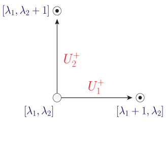
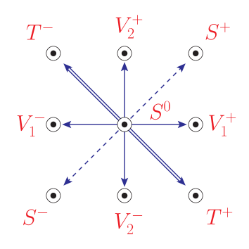
Figure 3: (Left) A diagrammatic description of the basic operators, $U^{+}_{1}$ and $U^{+}_{2}$ moving the integer-helicity point $[\lambda_{1},\lambda_{2}]$ to the integer-helicity point $[\lambda_{1}+1,\lambda_{2}]$ horizontally and to the integer-helicity point $[\lambda_{1},\lambda_{2}+1]$ vertically in the helicity-lattice space, respectively. Although not presented, the transitions moving down the integer-helicity point by one-step horizontally and vertically are dictated by the complex-conjugate operators, $U^{-}_{1}=(U^{+}_{1})^{*}$ and $U^{-}_{2}=(U^{+}_{2})^{*}$, respectively. (Right) A graphical description of the nine different transitions by the three scalar composite operators $S^{\pm}$ and $S^{0}$, four vector composite operators $V^{\pm}_{1}$ and $V^{\pm}_{2}$ and two tensor composite operators $T^{\pm}$.

4.2 Fermionic vertex operators

First, we consider the decay of a spin-0 particle $X$ into two spin-1/2 fermions, $M_{1}$ and $M_{2}$. The number of independent terms involving the $0\to 1/2+1/2$ two-body decay is $n\,[0,1/2]=2$, accounting for the two reduced helicity amplitudes, ${\cal C}^{\,0}_{\pm 1/2,\pm 1/2}$. After a little manipulation, we can find the following two covariant three-point operators,

$$P^{\pm}\,=\,\frac{1}{2m_{X}}\,(1\mp\kappa\gamma_{5})\qquad\leftrightarrow\qquad{\cal C}^{\,0}_{\pm 1/2,\pm 1/2}=\,\kappa\,,$$ (4.11)

with the $M_{1,2}$ speed $\kappa=\sqrt{1-4m^{2}/m^{2}_{X}}$ in the $X$RF.

Second, there are in general $n\,[1,1/2]=4$ independent terms for the $1\to 1/2+1/2$ decay mode, among which two terms take the same helicity combinations as in the $J=0$ case. The corresponding covariant three-point vertices are simply $\hat{k}_{\mu}\,P^{\pm}$ generating their corresponding reduced helicity amplitudes, ${\cal C}^{1}_{\pm 1/2,\pm 1/2}=-\kappa$, identical to $-{\cal C}^{\,0}_{\pm 1/2,\pm 1/2}$. The remaining two covariant vertices and their corresponding reduced helicity amplitudes are given by

$$W^{\pm}_{\mu}\,=\,\frac{1}{2\sqrt{2}m_{X}}(\pm\kappa\gamma_{\bot\mu}+\gamma_{\mu}\gamma_{5})\qquad\leftrightarrow\qquad{\cal C}^{1}_{\pm 1/2,\mp 1/2}=\,\pm\kappa\,,$$ (4.12)

with the orthogonal Dirac gamma matrix $\gamma_{\bot\mu}=\gamma_{\mu}+\frac{2m}{m_{X}\kappa}\,\hat{k}_{\mu}$.

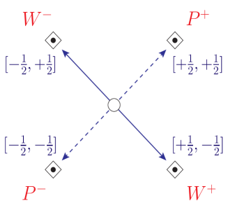
Figure 4: A diagrammatic description of the half-step transitions by the four fermionic operators, $P^{\pm}$ and $W^{\pm}$ from the original point $[0,0]$ to the four half-integer helicity points $[\mbox{\small$\pm\frac{1}{2}$},\mbox{\small$\pm\frac{1}{2}$}]$ and $[\mbox{\small$\pm\frac{1}{2}$},\mbox{\small$\mp\frac{1}{2}$}]$, respectively.

Properly combining the fermionic transition operators in Eqs. (4.11) and (4.12) and the bosonic transition operators in Eqs. (4.1), (4.2), (4.3) (4.4) and (4.5) enables us to reach every half-integer-helicity lattice point. To summarize, for any given integer $J$ and half-integer $s$, we can weave the covariant three-point vertex corresponding to every half-integer-helicity combination of $[\lambda_{1},\lambda_{2}]$ efficiently and systematically. The explicit form of the covariant fermionic three-point vertex constructed by weaving the fermionic as well as bosonic operators is to be presented in Section 5.

5 Weaving the covariant three-point vertices

Utilizing the nine composite bosonic operators and four basic fermionic operators worked out in Section 4, we weave the covariant three-point vertices explicitly. For that purpose, it is crucial to take into account that bosonic wave tensors are totally symmetric, traceless and divergence-free and the fermionic spinors satisfy

$$\gamma_{\alpha_{i}}u_{1}^{\alpha_{1}\cdots\alpha_{i}\cdots\alpha_{n}}(k_{1},\lambda_{1}) = \gamma_{\alpha_{i}}v_{2}^{\alpha_{1}\cdots\alpha_{i}\cdots\alpha_{n}}(k_{2},\lambda_{2})\,=\,\,0\,,$$ (5.1)

with the nonnegative integer $n=s-1/2$, so that every fermionic vertex involving $\gamma_{\alpha_{i}}$ or $\gamma_{\beta_{j}}$ with $i,j=1,\cdots,n$ can be effectively excluded. The $\mu$, $\alpha$ and $\beta$ four-vector indices in any covariant three-point vertex can be shuffled freely due to the totally symmetric properties of the wave tensors, and any term including $p_{\mu_{i}}$ for $i=1,\cdots J$ can be excluded effectively due to the divergence-free condition. Moreover, the same condition allows us to replace $k_{2\alpha_{j}}$ and $k_{1\beta_{j}}$ effectively by $-p_{\alpha_{j}}$ and $p_{\beta_{j}}$ for $j=1,\cdots n$.

As many indices of different types are involved in expressing a covariant three-point vertex especially for high-spin particles, we introduce the following compact square-bracket notations

$$[\,\hat{k}\,]^{n}\quad\ \ \rightarrow\quad(\hat{k}^{n})_{\mu_{1}\cdots\mu_{n}}=\hat{k}_{\mu_{1}}\cdots\hat{k}_{\mu_{n}}\,,$$ (5.2)

$$[\,\hat{p}\,]^{n}\quad\ \ \rightarrow\quad(\hat{p}^{n})_{\alpha_{1}\cdots\alpha_{n}}=\hat{p}_{\alpha_{1}}\cdots\hat{p}_{\alpha_{n}}\quad\mbox{and}\quad(\hat{p}^{n})_{\beta_{1}\cdots\beta_{n}}=\hat{p}_{\beta_{1}}\cdots\hat{p}_{\beta_{n}}\,,$$ (5.3)

$$[S^{\pm}]^{n}\quad\,\rightarrow\quad(S^{\pm})^{n}_{\alpha_{1}\cdots\alpha_{n}\beta_{1}\cdots\beta_{n}}=S^{\pm}_{\alpha_{1}\beta_{1}}\cdots S^{\pm}_{\alpha_{n}\beta_{n}}\,,$$ (5.4)

$$[V_{a}^{\pm}]^{n}\quad\rightarrow\quad(V_{a}^{\pm})^{n}_{\alpha_{1}\cdots\alpha_{n}\beta_{1}\cdots\beta_{n};\mu_{1}\cdots\mu_{n}}=V^{\pm}_{a\alpha_{1}\beta_{1};\mu_{1}}\cdots V^{\pm}_{a\alpha_{n}\beta_{n};\mu_{n}}\ \ \mbox{with}\ \ a=1,2\,,$$ (5.5)

$$[T^{\pm}]^{n}\quad\rightarrow\quad(T^{\pm})^{n}_{\alpha_{1}\cdots\alpha_{n}\beta_{1}\cdots\beta_{n};\mu_{1}\mu_{2}\cdots\mu_{2n-1}\mu_{2n}}=T^{\pm}_{\alpha_{1}\beta_{1};\mu_{1}\mu_{2}}\cdots T^{\pm}_{\alpha_{n}\beta_{n};\mu_{2n-1}\mu_{2n}}\,,$$ (5.6)

for a non-negative integer $n$. Obviously, the zeroth power ($n=0$) of any operator or normalized four momentum is set to be 1. We emphasize once more that any permutation of the $\alpha$, $\beta$ and $\mu$ four-vector indices can be regarded to be equivalent as eventually the vertex operators are to be coupled with the $X$ and $M_{1,2}$ wave tensors totally symmetric in the four-vector indices.

5.1 Bosonic three-point vertices

In the integer $s$ case, any helicity lattice point where both $\lambda_{1}$ and $\lambda_{2}$ are even or odd can be reached through a sequence of diagonal transitions by the scalar composite operators $S^{\pm}$ and $S^{0}$ and the tensor composite operators $T^{\pm}$. In fact, a little algebraic manipulation leads to the following expression for the covariant three-point vertex

$$[\,{\cal H}^{J,s}_{ii[\lambda_{1},\lambda_{2}]}\,]\,=\,[\,\hat{k}\,|^{J-2|\lambda_{-}|}\,[S^{0}]^{s-|\lambda_{+}|-|\lambda_{-}|}\,[S^{\hat{\lambda}_{+}}]^{|\lambda_{+}|}\,[T^{\hat{\lambda}_{-}}|^{|\lambda_{-}|}\,,$$ (5.7)

in an operator form with two helicity combinations, $\lambda_{+}=(\lambda_{1}+\lambda_{2})/2$ and $\lambda_{-}=(\lambda_{1}-\lambda_{2})/2$, and their signs, $\hat{\lambda}_{+}={\rm sign}(\lambda_{+})$ and $\hat{\lambda}_{-}={\rm sign}(\lambda_{-})$. We note that both $\lambda_{+}$ and $\lambda_{-}$ take integer values. The subscript $ii$ implies that both $\lambda_{+}$ and $\lambda_{-}$ take integer values.

On the other hand, any helicity lattice point where $\lambda_{1}$ and $\lambda_{2}$ are even and odd and vice versa can be reached through a sequence of diagonal transitions by the scalar composite operators $S^{\pm}$ and $S^{0}$ and the tensor composite operators $T^{\pm}$ followed by a proper vertical or horizontal transition among the vector composite operators $V^{\pm}_{1}$ and $V^{\pm}_{2}$. Explicitly, we have the following expression with half-integer $\lambda_{+}$ and $\lambda_{-}$ for the three-point vertex

$$[\,{\cal H}^{J,s}_{hh[\lambda_{1},\lambda_{2}]}\,]\,=\,[\,\hat{k}\,|^{J-2|\lambda_{-}|}\,[S^{0}]^{s-|\lambda_{+}|-|\lambda_{-}|}\,[\,\delta_{\hat{\lambda}_{+},\hat{\lambda}_{-}}\,V_{1}^{\hat{\lambda}_{+}}+\delta_{\hat{\lambda}_{+},-\hat{\lambda}_{-}}V_{2}^{\hat{\lambda}_{+}}\,]\,[S^{\hat{\lambda}_{+}}]^{|\lambda_{+}|-1/2}\,[T^{\hat{\lambda}_{-}}|^{|\lambda_{-}|-1/2}\,,$$ (5.8)

with two non-negative integer values of $|\lambda_{\pm}|-1/2$ in this case. The subscript $hh$ implies that both $\lambda_{+}$ and $\lambda_{-}$ take half-integer values.

5.2 Fermionic three-point vertices

In the half-integer $s$ case with two fermions $M_{1}$ and $M_{2}$, the helicity combinations can be categorized into two classes. One is when the helicity sum $[\lambda_{1}+\lambda_{2}]$ and the helicity difference $[\lambda_{1}-\lambda_{2}]$ are odd and even with a half-integer $\lambda_{+}$ and an integer $\lambda_{-}$, to be denoted by the notation $hi$. The other is when the helicity sum and difference are even and odd with an integer $\lambda_{+}$ and a half-integer $\lambda_{-}$, to be denoted by the notation $ih$. Taking a proper half-integer helicity transition as described in Figure 4 followed by a sequence of integer helicity transitions, we can obtain the following expression of the fermionic three-point vertex with the helicities $\lambda_{1}$ and $\lambda_{2}$ as

$$[\,{\cal H}^{J,s}_{hi[\lambda_{1},\lambda_{2}]}\,]\,=\,[\,\hat{k}\,]^{J-2|\lambda_{-}|}\,[S^{0}]^{s-|\lambda_{+}|-|\lambda_{-}|}\,[P^{\hat{\lambda}_{+}}]\,[S^{\hat{\lambda}_{+}}]^{|\lambda_{+}|-1/2}\,[T^{\hat{\lambda}_{-}}]^{|\lambda_{-}|}\,,$$ (5.9)

involving a fermionic scalar operator $P^{\pm}$ for half-integer $\lambda_{+}$ and integer $\lambda_{-}$ and

$$[\,{\cal H}^{J,s}_{ih[\lambda_{1},\lambda_{2}]}\,]\,=\,[\,\hat{k}\,]^{J-2|\lambda_{-}|}\,[S^{0}]^{s-|\lambda_{+}|-|\lambda_{-}|}\,[W^{\hat{\lambda}_{-}}]\,[S^{\hat{\lambda}_{+}}]^{|\lambda_{+}|}\,[T^{\hat{\lambda}_{-}}]^{|\lambda_{-}|-1/2}\,,$$ (5.10)

involving a fermionic vector operator $W^{\pm}$ for integer $\lambda_{+}$ and half-integer $\lambda_{-}$. The subscript $hi$ ($ih$) implies that $\lambda_{+}$ takes a half-integer (an integer) value and $\lambda_{-}$ an integer (a half-integer) value.

To conclude, in both the integer and half-integer spin $s$ cases, the general form of any covariant three-point vertex $\Gamma_{\alpha\beta;\mu}$ for given $J$ and $s$ is a linear combination of all the allowed helicity-specific three-point vertices. The succinct operator form of the covariant three-point vertex is given by

$$[\,\Gamma\,]\,=\,\left\{\begin{array}[]{ll}\sum^{s}_{\lambda_{1,2}=-s}\,\left[\,c^{J,s}_{ii[\lambda_{1},\lambda_{2}]}\,[\,{\cal H}^{J,s}_{ii[\lambda_{1},\lambda_{2}]}\,]+c^{J,s}_{hh[\lambda_{1},\lambda_{2}]}\,[\,{\cal H}^{J,s}_{hh[\lambda_{1},\lambda_{2}]}\,]\,\right]&\ \ \mbox{for an integer $s$}\,,\\[14.22636pt] \sum^{s}_{\lambda_{1,2}=-s}\,\left[\,c^{J,s}_{hi[\lambda_{1},\lambda_{2}]}\,[\,{\cal H}^{J,s}_{hi[\lambda_{1},\lambda_{2}]}\,]+c^{J,s}_{ih[\lambda_{1},\lambda_{2}]}\,[\,{\cal H}^{J,s}_{ih[\lambda_{1},\lambda_{2}]}\,]\,\right]&\ \ \mbox{for a half-integer $s$}\,,\end{array}\right.$$ (5.13)

with the constraint $|\lambda_{1}-\lambda_{2}|\leq J$, i.e., $J-2|\lambda_{-}|\geq 0$, where the helicity-specific coefficients, $c^{J,s}_{x[\lambda_{1},\lambda_{2}]}$ with $x=ii,hh,hi,hi$ depend only on the $X$ and $M_{1,2}$ masses. We claim that the expression (5.13) along with the helicity-specific vertices in Eqs. (5.7), (5.8), (5.9) and (5.10) is the key result of the present work. Although it is originally deduced from the comparison with the helicity amplitudes in the $X$RF, the form is valid in every reference frame because of its Lorentz-covariant form.

5.3 Massless case

In the case with massless $M_{1,2}$ of spin $s$, the physically-allowed helicity values are $\pm s$. Furthermore, the five scalar and vector operators $S^{0}$ and $V^{\pm}_{1,2}$ are vanishing as they are proportional to $m^{2}$ and $m$, respectively. Therefore, the helicity-specific vertices could survive only when $\lambda_{1}=\lambda_{2}=\pm s$ or $\lambda_{1}=-\lambda_{2}=\pm s$. These combinations satisfy $s-|\lambda_{+}|+|\lambda_{-}|=0$. In addition, in the opposite helicity case, the $X$ spin $J$ cannot be smaller than $2s$. Consequently, in the $m=0$ case, there could exist at most four independent terms in both the bosonic and fermionic cases, as counted in Eq. (2.12).

In the bosonic case with an integer $s$, the bosonic covariant three-point vertex is given in an operator form by

$$[\,\Gamma\,] = c^{J,s}_{ii[+s,+s]}\,[\,k\,]^{J}\,[S^{+}]^{s}+c^{J,s}_{ii[-s,-s]}\,[\,k\,]^{J}\,[S^{-}]^{s}$$ (5.14)

$$+ \theta(J-2s)\,\left\{\,c^{J,s}_{ii[+s,-s]}\,[\,k\,]^{J-2s}\,[T^{+}]^{s}+c^{J,s}_{ii[-s,+s]}\,[\,k\,]^{J-2s}\,[T^{-}]^{s}\,\right\}\,,$$

where the last two terms survive only when $J\geq 2s$, as denoted by the step function $\theta(J-2s)=1$ for $J\geq 2s$ and $0$ for $J<2s$. On the other hand, in the fermionic case with a half-integer $s$, the fermionic covariant three-point vertex is given in an operator form as

$$[\,\Gamma\,] = c^{J,s}_{hi[+s,+s]}\,[\,k\,]^{J}\,[P^{+}]\,[S^{+}]^{s-1/2}+c^{J,s}_{hi[-s,-s]}\,[\,k\,]^{J}\,[P^{-}]\,[S^{-}]^{s-1/2}$$ (5.15)

$$+ \theta(J-2s)\,\left\{\,c^{J,s}_{ih[+s,-s]}\,[\,k\,]^{J-2s}\,[W^{+}]\,[T^{+}]^{s-1/2}+c^{J,s}_{ih[-s,+s]}\,[\,k\,]^{J-2s}\,[W^{-}]\,[T^{-}]^{s-1/2}\,\right\}\,.$$

The results in Eqs. (5.14) and (5.15) are consistent with those derived in Ref. [30].

5.4 Identical particle relation: Bose or Fermi symmetry

If two particles $M_{1}$ and $M_{2}$ are identical, the state of the two-particle system must be symmetric or antisymmetric under the interchange of two integer or half-integer spin particles. In this subsection we work out the constraints on the covariant three-point vertex imposed by the Bose or Fermi symmetry.

In the bosonic case with two identical particles of an integer spin $s$, the covariant three-point vertex tensor $\Gamma_{\alpha\beta;\mu}$ must be symmetric under the interchange of $M_{1}$ and $M_{2}$ due to Bose symmetry as

$$\Gamma_{\alpha_{1}\cdots\alpha_{s},\beta_{1}\cdots\beta_{s};\,\mu_{1}\cdots\mu_{J}}(p,k)\,\,=\,\,\Gamma_{\beta_{1}\cdots\beta_{s},\alpha_{1}\cdots\alpha_{s};\,\mu_{1}\cdots\mu_{J}}(p,-k)\,,$$ (5.16)

under the transformations

$$\alpha_{i}\quad\leftrightarrow\quad\beta_{j}\quad\mbox{and}\quad k_{1}\quad\leftrightarrow\quad k_{2}\,,$$ (5.17)

for any pair of $i,j=1,\cdots,s$, leaving $p=k_{1}+k_{2}$ invariant but changing the sign of $k$ as $k\to-k$. Combining the index and momentum interchanges with the interchange of the $M_{1}$ and $M_{2}$ helicities, the helicity-specific three-point vertices transform under the Bose symmetrization as

$$[\,{\cal H}^{J,s}_{ii[\lambda_{1},\lambda_{2}]}\,]\quad\leftrightarrow\quad(-1)^{J}\,[\,{\cal H}^{J,s}_{ii[\lambda_{2},\lambda_{1}]}\,]\quad\mbox{and}\quad[\,{\cal H}^{J,s}_{hh[\lambda_{1},\lambda_{2}]}\,]\quad\leftrightarrow\quad-(-1)^{J}\,[\,{\cal H}^{J,s}_{hh[\lambda_{2},\lambda_{1}]}\,]\,,$$ (5.18)

leading to the constraints on the helicity-specific coefficients as

$$c^{J,s}_{ii[\lambda_{1},\lambda_{2}]}\,=\,(-1)^{J}\,c^{J,s}_{ii[\lambda_{2},\lambda_{1}]}\quad\mbox{and}\quad c^{J,s}_{hh[\lambda_{1},\lambda_{2}]}\,=\,-(-1)^{J}\,c^{J,s}_{hh[\lambda_{2},\lambda_{1}]}\,.$$ (5.19)

One observation is that the diagonal $ii$ and $hh$ elements with $\lambda_{1}=\lambda_{2}$ vanish for odd $J$ and even $J$, respectively. Another observation is that any spin-$1$ ($J=1$) particle cannot decay into two identical massless spin-1 particles, as the coefficient of the only allowed terms $c^{1,1}_{ii[\lambda,\lambda]}$ vanish, as proven more than seventy years ago [43, 44]. We note that the so-called Landau-Yang theorem is generalized to the case with any values of $J$ and $s$ [30].

In the fermionic case with two identical fermions of a half-integer spin $s$, interchanging two identical massless fermions, i.e., taking the opposite fermion flow line [46, 47], we can rewrite the helicity amplitude of the decay $X\to ff$ with a massless fermion $M=f$ as

$$\tilde{\cal M}^{X\to ff}_{\sigma;\lambda_{1},\lambda_{2}} = \bar{u}_{2}^{\beta}(k_{2},\lambda_{2})\,\,\Gamma^{\mu}_{\beta,\alpha}(p,-k)\,\,v_{1}^{\alpha}(k_{1},\lambda_{1})\,\,\epsilon_{\mu}(p,\sigma)$$ (5.20)

$$= v_{1}^{\alpha T}(k_{1},\lambda_{1})\,\,\Gamma^{\mu T}_{\beta,\alpha}(p,-k)\,\,\bar{u}_{2}^{\beta T}(k_{2},\lambda_{2})\,\,\epsilon_{\mu}(p,\sigma)\,,$$

with the superscript $T$ denoting the transpose of the matrix. Introducing the charge-conjugation operator $C$ satisfying $C^{\dagger}=C^{-1}$ and $C^{T}=-C$ relating the $v$ spinor to the $u$ spinor as

$$v^{\alpha}(k,\lambda)=C\bar{u}^{\alpha T}(k,\lambda)\,,$$ (5.21)

with $\bar{u}=u^{\dagger}\gamma^{0}$, we can rewrite the amplitude as

$$\tilde{\cal M}^{X\to ff}_{\sigma;\lambda_{1},\lambda_{2}} = -\bar{u}_{1}^{\beta}(k_{1},\lambda_{1})\,\,C\,\Gamma^{\mu T}_{\beta,\alpha}(p,-k)\,C^{-1}\,\,v_{2}^{\alpha}(k_{2},\lambda_{2})\,\,\epsilon_{\mu}(p,\sigma)\,.$$ (5.22)

Since Fermi statistics requires $\tilde{\cal M}=-{\cal M}$, the three-point vertex tensor must satisfy the relation

$$C\,\Gamma^{\mu T}_{\beta,\alpha}(p,-k)\,C^{-1}\,=\,\Gamma^{\mu}_{\alpha,\beta}(p,k)\,,$$ (5.23)

which enables us to classify all the allowed terms systematically [48, 49, 41].

The basic relation for the charge-conjugation invariance of the Dirac equation is $C\,\gamma^{T}_{\mu}\,C^{-1}=-\gamma_{\mu}$ with a unitary matrix $C$. Repeatedly using the basic relation, we can derive

$$\Gamma^{c}\,\equiv\,C\,\Gamma^{T}\,C^{-1}\,=\,\epsilon_{C}\,\Gamma\quad\mbox{with}\quad\epsilon_{C}=\left\{\begin{array}[]{lll}+1&\mbox{for}&\Gamma=1,\gamma_{5},\gamma_{\mu}\gamma_{5}\,,\\[5.69054pt] -1&\mbox{for}&\Gamma=\gamma_{\mu}\,,\end{array}\right.$$ (5.26)

There are no further independent terms as any other operator can be replaced by a linear combination of $1,\,\gamma_{5},\,\gamma_{\mu}$, and $\gamma_{\mu}\gamma_{5}$ by use of the so-called Gordon identities, when coupled to the $u$ and $v$ spinors.

Consequently, according to all the transformation properties of covariant three-point vertex operators worked out above, the helicity-specific three-point vertices transform under the Fermi symmetrization as

$${\cal H}^{J,s}_{hi[\lambda_{1},\lambda_{2}]}\quad\leftrightarrow\quad(-1)^{J}\,{\cal H}^{J,s}_{hi[\lambda_{2},\lambda_{1}]}\quad\mbox{and}\quad{\cal H}^{J,s}_{ih[\lambda_{1},\lambda_{2}]}\quad\leftrightarrow\quad-(-1)^{J}\,{\cal H}^{J,s}_{ih[\lambda_{2},\lambda_{1}]}\,,$$ (5.27)

leading to the constraints on the helicity-specific coefficients as

$$c^{J,s}_{hi[\lambda_{1},\lambda_{2}]}\,=\,(-1)^{J}\,c^{J,s}_{hi[\lambda_{2},\lambda_{1}]}\quad\mbox{and}\quad c^{J,s}_{ih[\lambda_{1},\lambda_{2}]}\,=\,-(-1)^{J}\,c^{J,s}_{ih[\lambda_{2},\lambda_{1}]}\,.$$ (5.28)

One observation is that the diagonal $hi$ and $ih$ elements with $\lambda_{1}=\lambda_{2}$ vanish for odd $J$ and even $J$, respectively, as in the bosonic case.

5.5 Off-shell electromagnetic gauge-invariant vertices

Due to the electromagnetic (EM) gauge invariance, any off-shell photon couples to a conserved current. Therefore, in any time-like photon exchange process involving the $\gamma^{*}M_{1}M_{2}$ vertex, the off-shell photon can be treated as a spin-1 particle of mass $m_{X}=\sqrt{p^{2}}$. Moreover, the covariant three-point $\gamma^{*}M_{1}M_{2}$ vertex can be cast into a manifestly EM gauge-invariant form [34, 41] as

$$\Gamma^{\mu}_{{\rm EM}\,\,\alpha,\beta}\,=\,p^{2}\,\Gamma^{\mu}_{\alpha,\beta}-(\,p\cdot\Gamma_{\alpha,\beta}\,)\,p^{\mu}\,,$$ (5.29)

automatically satisfying the current conservation condition $p_{\mu}\Gamma^{\mu}_{{\rm EM}\,\alpha,\beta}=p\cdot\Gamma_{{\rm EM}\,\alpha,\beta}=0$.

The IP condition on the redefined EM gauge-invariant three-point vertex is identical to that on the original three-point vertex as the momentum $p$ is invariant under Bose or Fermi symmetry. Note that the case with an off-shell spin-$J$ particle coupled to a conserved tensor current can be treated in a similar manner as in the off-shell photon case.

6 Various specific examples

First, we consider the decay of a spin-$0$ particle into two spin-$s$ particles. In this case, the restriction $|\lambda_{1}-\lambda_{2}|\leq J=0$ forces $\lambda_{1}=\lambda_{2}=\lambda$ to be satisfied so that the three-point vertex consists of the $n\,[0,s]=2s+1$ independent terms of the form

$$[\,{\cal H}^{0,s}_{ii[\lambda,\lambda]}\,]\,=\,[S^{0}]^{s-|\lambda|}\,[S^{\hat{\lambda}}]^{|\lambda|}\,,$$ (6.1)

with $\lambda$ varying from $-s$ to $s$ and $\hat{\lambda}={\rm sign}(\lambda)$ in the bosonic case with a non-negative integer $s$, and

$$[\,{\cal H}^{0,s}_{hi[\lambda,\lambda]}\,]\,=\,[S^{0}]^{s-|\lambda|}[P^{\hat{\lambda}}][S^{\hat{\lambda}}]^{|\lambda|-1/2}\,,$$ (6.2)

in the fermionic case with a positive half-integer $s$. Note that the three-point vertices do not change in number and form even in the IP case with $J=0$, as all the scalar composite operators, $S^{0}$, $S^{\pm}$ and $P^{\pm}$, are symmetric under Bose and Fermi symmetry transformations.

Second, we consider the case with $J=1$. There exist $n\,[1,s]=6s+1$ independent terms decomposed into two classes. One class with $2s+1$ terms is when two helicities are identical, i.e., $\lambda_{1}=\lambda_{2}$. The corresponding helicity-specific vertex is given by

$$[\,{\cal H}^{1,s}_{ii[\lambda,\lambda]}\,]\,=\,[\hat{k}]\,[S^{0}]^{s-|\lambda|}\,[S^{\hat{\lambda}}]^{|\lambda|}\,=\,[\hat{k}]\,[\,{\cal H}^{0,s}_{ii[\lambda,\lambda]}\,]\,,$$ (6.3)

in the bosonic case, and

$$[\,{\cal H}^{1,s}_{hi[\lambda,\lambda]}\,]\,=\,[\hat{k}]\,[S^{0}]^{s-|\lambda|}[P^{\hat{\lambda}}][S^{\hat{\lambda}}]^{|\lambda|-1/2}\,=\,[\hat{k}]\,[\,{\cal H}^{0,s}_{hi[\lambda,\lambda]}\,]\,,$$ (6.4)

in the fermionic case. It is noteworthy that all the helicity-specific vertices in Eqs. (6.3) and (6.4) vanish in the IP case, as the operator $[\hat{k}]$ is antisymmetric under Bose and Fermi symmetrization. The other class with $4s$ independent terms is when the difference of two helicities are $\pm 1$, i.e., $\lambda_{1}=\lambda_{2}\pm 1$. The corresponding helicity-specific bosonic vertex is given by

$$[\,{\cal H}^{1,s}_{hh[\lambda,\lambda\mp 1]}\,]\,=\,[S^{0}]^{s-|\lambda_{+}|-1/2}\,[\,\delta_{\hat{\lambda}_{+},\pm}V^{\pm}_{1}+\delta_{\hat{\lambda}_{+},\mp}V^{\mp}_{2}\,]\,[S^{\hat{\lambda}_{+}}]^{|\lambda_{+}|-1/2}\,,$$ (6.5)

with $\lambda_{+}=\lambda\mp 1/2$ and the constraint $|\lambda_{+}|\leq s-1/2$, and the helicity-specific fermionic vertex by

$$[\,{\cal H}^{1,s}_{ih[\lambda,\lambda\mp 1]}\,]\,=\,[S^{0}]^{s-|\lambda_{+}|-1/2}\,[W^{\pm}]\,[S^{\hat{\lambda}_{+}}]^{|\lambda_{+}|}\,,$$ (6.6)

with $\lambda_{+}=\lambda\mp 1/2$ and the constraint $|\lambda_{+}|\leq s-1/2$. In the IP case with two identical particles ($M_{1}=M_{2}$), the covariant three-point vertex in the bosonic case is

$$[\,{\cal H}^{1,s}_{hh[\lambda,\lambda\mp 1]}\,]_{\rm IP}\,=\,\frac{1}{2}\,[S^{0}]^{s-|\lambda_{+}|-1/2}\,[\,\delta_{\hat{\lambda}_{+},\pm}(V^{\pm}_{1}+V^{\pm}_{2})+\delta_{\hat{\lambda}_{+},\mp}(V^{\mp}_{1}+V^{\mp}_{2})\,]\,[S^{\hat{\lambda}_{+}}]^{|\lambda_{+}|-1/2}\,,$$ (6.7)

with $(V^{\pm}_{1}+V^{\pm}_{2})_{\alpha,\beta;\mu}=(m/m_{X})\,[\,(g_{\bot\alpha\mu}\hat{p}_{\beta}+g_{\bot\beta\mu}\hat{p}_{\alpha})\pm i(\langle\alpha\mu\hat{p}\hat{k}\rangle\hat{p}_{\beta}-\langle\beta\mu\hat{p}\hat{k}\rangle\hat{p}_{\alpha})\,]$, and the covariant three-point vertex in the fermionic case is

$$[\,{\cal H}^{1,s}_{ih[\lambda,\lambda\mp 1]}\,]_{\rm IP}\,=\,\frac{1}{2}\,[S^{0}]^{s-|\lambda_{+}|-1/2}\,[W^{+}+W^{-}]\,[S^{\hat{\lambda}_{+}}]^{|\lambda_{+}|}\,,$$ (6.8)

with $(W^{+}+W^{-})_{\mu}=\gamma_{\mu}\gamma_{5}/\sqrt{2}m_{X}$ which is of a typical axial-vector type. These results are consistent with those in Ref. [41]. Explicitly, for $J=1$ and $s=1/2$, the surviving three-point vertex is simply proportional to $\gamma_{\mu}\gamma_{5}$. For $J=1$ and $s=1$, the three-point vertex, which can be applied to the model-independent description of the anomalous $VZZ$ vertices with virtual $V=\gamma,Z$ or on-shell $Z^{\prime}$ [45, 50, 51, 52, 53], is composed of two independent terms $(V^{\pm}_{1}+V^{\pm}_{2})_{\alpha\beta;\mu}$ proportional to the mass $m$ so that it is vanishing in the massless limit.

Third, we consider the case with $J=2$. The number of independent terms are $n\,[2,0]=1$ for $s=0$ and $n\,[2,s]=10s-1$ for $s>0$, which are decomposed into two classes. The first class with $6s+1$ terms is when two helicities are identical, i.e., $\lambda_{1}=\lambda_{2}$. The corresponding helicity-specific vertices are given by

$$[\,{\cal H}^{2,s}_{ii[\lambda,\lambda]}\,]\,=\,[\hat{k}]^{2}\,[\,{\cal H}^{0,s}_{ii[\lambda,\lambda]}\,]\ \ \mbox{and}\ \ [\,{\cal H}^{2,s}_{hh[\lambda,\lambda\pm 1]}\,]\,=\,[\hat{k}]\,[\,{\cal H}^{1,s}_{hh[\lambda,\lambda\pm 1]}\,]\,,$$ (6.9)

in the bosonic case, and

$$[\,{\cal H}^{2,s}_{hi[\lambda,\lambda]}\,]\,=\,[\hat{k}]^{2}\,[\,{\cal H}^{0,s}_{hi[\lambda,\lambda]}\,]\ \ \mbox{and}\ \ [\,{\cal H}^{2,s}_{ih[\lambda,\lambda\pm 1]}\,]\,=\,[\hat{k}]\,[\,{\cal H}^{1,s}_{ih[\lambda,\lambda\pm 1]}\,]\,,$$ (6.10)

in the fermionic case. They constitute $2s+1$ and $4s$ independent covariant three-point vertices both in the bosonic and fermion cases. The second class with $2(2s-1)$ independent terms appear for the helicity difference of $\lambda_{1}-\lambda_{2}=\pm 2$. The corresponding helicity-specific vertices are given by

$$[\,{\cal H}^{2,s}_{ii[\lambda,\lambda\mp 2]}\,]\,=\,[S^{0}]^{s-|\lambda_{+}|-1}\,\,[S^{\hat{\lambda}_{+}}|^{|\lambda_{+}|}\,\,[T^{\pm}]\,,$$ (6.11)

in the bosonic case with $\lambda_{+}=\lambda\mp 1$, and

$$[\,{\cal H}^{2,s}_{hi[\lambda,\lambda\mp 2]}\,]\,=\,[S^{0}]^{s-|\lambda_{+}|-1}\,\,[P^{\hat{\lambda}_{+}}]\,\,[S^{\hat{\lambda}_{+}}]^{|\lambda_{+}|-1/2}\,\,[T^{\pm}]\,,$$ (6.12)

in the fermionic case with $\lambda_{+}=\lambda\mp 1$. The $J=2$ covariant three-point vertices can be adopted for studying the massive KK graviton or off-shell graviton interactions with two spin-$s$ particles of equal mass $m$.

Now, we demonstrate the power of the algorithm by explicitly working out all the characteristic features of four specific decay modes with the $[J,s]$ values of $[0,0]$, $[0,1]$, $[1,1]$ and $[2,1]$ in the integer spin $s$ case. We fully write down the number of independent terms $n\,[J,s]$, the allowed helicity assignments $(\lambda_{1},\lambda_{2})$, the helicity-specific covariant three-point vertices $[\,{\cal H}^{J,s}_{[\lambda_{1},\lambda_{2}]}\,]$ in an operator form and their corresponding reduced helicity amplitudes ${\cal C}^{J}_{\lambda_{1},\lambda_{2}}$ as well as the helicity-specific covariant three-point vertices $[\,{\cal H}^{J,s}_{{\rm IP}[\lambda_{1},\lambda_{2}]}\,]$ in an operator form and the number of independent terms $n\,[J,s]_{\rm IP}$ in the IP case. The results are summarized succinctly in Table 1.

Integer spin-$s$ case
$(J,s)$	$n\,[J,s]$	$(\lambda_{1},\lambda_{2})$	$[\,H^{J,s}_{[\lambda_{1},\lambda_{2}]}\,]$	${\cal C}^{J}_{\lambda_{1},\lambda_{2}}$	$[\,H^{J,s}_{{\rm IP}[\lambda_{1},\lambda_{2}]}\,]$	$n\,[J,s]_{\rm IP}$
$(0,0)$	$1$	$(0,0)$	$[\,1\,]$	$1$	$[1]$	$1$
$(0,1)$	$3$	$(\pm 1,\pm 1)$	$[\,S^{\pm}\,]$	$1$	$[S^{\pm}]$	$3$
		$(0,0)$	$[\,S^{0}\,]$	$-\kappa^{2}$	$[S^{0}]$
$(1,1)$	$7$	$(\pm 1,\pm 1)$	$[\,\hat{k}\,][S^{\pm}]$	$-1$	$-$	$2$
		$(0,0)$	$[\,\hat{k}\,][S^{0}]$	$\kappa^{2}$	$-$
		$(\pm 1,0)$	$[V_{1}^{\pm}]$	$\kappa$	$\frac{1}{2}[V^{\pm}_{1}+V^{\pm}_{2}]$
		$(0,\pm 1)$	$[V_{2}^{\pm}]$	$-\kappa$
$(2,1)$	$9$	$(\pm 1,\pm 1)$	$[\,\hat{k}\,]^{2}[S^{\pm}]$	$1$	$[\,\hat{k}\,]^{2}\,[S^{\pm}]$	$6$
		$(0,0)$	$[\,\hat{k}\,]^{2}\,[S^{0}]$	$-\kappa^{2}$	$[\,\hat{k}\,]^{2}\,[S^{0}]$
		$(\pm 1,0)$	$[\,\hat{k}\,][V_{1}^{\pm}]$	$-\kappa$	$\frac{1}{2}\,[\,\hat{k}\,]\,[V^{\pm}_{1}-V^{\pm}_{2}]$
		$(0,\pm 1)$	$[\,\hat{k}\,][V_{2}^{\pm}]$	$\kappa$
		$(\pm 1,\mp 1)$	$[T^{\pm}]$	$1$	$\frac{1}{2}\,[T^{+}+T^{-}]$

Table 1: Specific examples in the integer spin $s$ case. Listed are the number of independent terms $n\,[J,s]$, the allowed helicity assignments $(\lambda_{1},\lambda_{2})$, the helicity-specific covariant three-point vertices $[\,H^{J,s}_{[\lambda_{1},\lambda_{2}]}\,]$ in an operator form and their corresponding reduced helicity amplitudes ${\cal C}^{J}_{\lambda_{1},\lambda_{2}}$, the helicity-specific covariant three-point vertex $[\,H^{J,s}_{{\rm IP}[\lambda_{1},\lambda_{2}]}\,]$ in an operator form and the number of independent terms $n\,[J,s]_{\rm IP}$ in the IP case for a few integer $J$ and integer $s$ assignments. This table is presented for demonstrating the effectiveness of the algorithm for weaving and characterizing the covariant triple vertices.

Using the algorithm for weaving the general covariant three-point vertices by explicitly evaluating three specific decay modes with the $[J,s]$ values of $[0,1/2]$, $[1,1/2]$ and $[2,1/2]$ in the half-integer spin $s$ case. The results are summarized in Table 2.

Half-integer spin-$s$ case
$(J,s)$	$n\,[J,s]$	$(\lambda_{1},\lambda_{2})$	$[\,H^{J,s}_{[\lambda_{1},\lambda_{2}]}\,]$	${\cal C}^{J}_{\lambda_{1},\lambda_{2}}$	$[\,{\cal H}^{J,s}_{{\rm IP}[\lambda_{1},\lambda_{2}]}\,]$	$n\,[J,s]_{\rm IP}$
$(0,1/2)$	$2$	$(\pm 1/2,\pm 1/2)$	$P^{\pm}$	$\kappa$	$[P^{\pm}]$	$2$
$(1,1/2)$	$4$	$(\pm 1/2,\pm 1/2)$	$[\,\hat{k}][P^{+}]$	$-\kappa$	$-$	$1$
		$(\pm 1/2,\mp 1/2)$	$[W^{\pm}]$	$\pm\kappa$	$[W^{+}+W^{-}]$
$(2,1/2)$	$4$	$(\pm 1/2,\pm 1/2)$	$[\,\hat{k}\,]^{2}[P^{\pm}]$	$\kappa$	$[\,\hat{k}\,]^{2}\,[P^{\pm}]$	$3$
		$(\pm 1/2,\mp 1/2)$	$[\,\hat{k}\,][W^{\pm}]$	$\mp\kappa$	$[\,\hat{k}]\,[W^{+}-W^{-}]$

Table 2: Specific examples in the half-integer spin $s$ case. Listed are the number of independent terms $n\,[J,s]$, the allowed helicity assignments $(\lambda_{1},\lambda_{2})$, the helicity-specific covariant triple vertices $[\,H^{J,s}_{[\lambda_{1},\lambda_{2}]}\,]$ in an operator form and their corresponding reduced helicity amplitudes ${\cal C}^{J}_{\lambda_{1},\lambda_{2}}$, the helicity-specific covariant three-point vertex $[\,H^{J,s}_{{\rm IP}[\lambda_{1},\lambda_{2}]}\,]$ in an operator form and the number of independent terms $n\,[J,s]_{\rm IP}$ in the IP case for a few integer $J$ and half-integer $s$ assignments.

7 Conclusions

We have developed an efficient algorithm for compactly weaving all the covariant three-point vertices for the decay of a spin-$J$ particle $X$ of mass $m_{X}$ into two particles $M_{1,2}$ with equal mass $m$ and spin $s$. For this development, we have made good use of the closely-related equivalence between the helicity formalism and the covariant formulation for identifying the basic building blocks and composite three-point vertex operators for constructing all the covariant three-point vertices. All the helicity-specific covariant three-point vertices are presented in an operator form in Eqs. (5.7) and (5.8) in the bosonic case and in Eqs. (5.9) and (5.10) in the fermionic case, respectively. The massless ($m=0$) case could be worked out straightforwardly and the (anti)symmetrization of the covariant three-point vertices required by Bose or Fermi spin statistics of two identical final-state particles could be made systematically in the context of this efficient algorithm.

This general algorithm for constructing the effective covariant three-point vertices is expected to be very useful in studying various phenomenological aspects such as the indirect and direct searches of high-spin dark matter particles and the pair production of high-spin particles at high energy colliders.

Naturally, it will be valuable to extend our algorithm for dealing with the general case when all the three particles have different masses and spins. It is also an interesting question whether the bosonic and fermionic cases can be synthesized in a unified framework, covering various forms of wave tensors for particles of any spin. These generalization and synthesis are presently under study and the results will be reported separately.

References

- [1] S. L. Glashow, “Partial Symmetries of Weak Interactions,” Nucl. Phys. 22 (1961), 579-588 doi:10.1016/0029-5582(61)90469-2.
- [2] S. Weinberg, “A Model of Leptons,” Phys. Rev. Lett. 19 (1967), 1264-1266 doi:10.1103/PhysRevLett.19.1264.
- [3] A. Salam, “Weak and Electromagnetic Interactions,” Conf. Proc. C 680519 (1968), 367-377 doi:10.1142/9789812795915_0034.
- [4] H. Fritzsch, M. Gell-Mann and H. Leutwyler, “Advantages of the Color Octet Gluon Picture,” Phys. Lett. B 47 (1973), 365-368 doi:10.1016/0370-2693(73)90625-4.
- [5] G. Aad et al. [ATLAS], “Observation of a new particle in the search for the Standard Model Higgs boson with the ATLAS detector at the LHC,” Phys. Lett. B 716 (2012), 1-29 doi:10.1016/j.physletb.2012.08.020 [arXiv:1207.7214 [hep-ex]].
- [6] S. Chatrchyan et al. [CMS], “Observation of a New Boson at a Mass of 125 GeV with the CMS Experiment at the LHC,” Phys. Lett. B 716 (2012), 30-61 doi:10.1016/j.physletb.2012.08.021 [arXiv:1207.7235 [hep-ex]].
- [7] P. A. Zyla et al. [Particle Data Group], “Review of Particle Physics,” PTEP 2020 (2020) no.8, 083C01 doi:10.1093/ptep/ptaa104.
- [8] V. Shklyar, H. Lenske and U. Mosel, “Spin-5/2 fields in hadron physics,” Phys. Rev. C 82 (2010), 015203 doi:10.1103/PhysRevC.82.015203 [arXiv:0912.3751 [hep-ph]].
- [9] E. Bergshoeff, D. Grumiller, S. Prohazka and J. Rosseel, “Three-dimensional Spin-3 Theories Based on General Kinematical Algebras,” JHEP 01 (2017), 114 doi:10.1007/JHEP01(2017)114 [arXiv:1612.02277 [hep-th]].
- [10] S. Jafarzade, A. Koenigstein and F. Giacosa, “Phenomenology of = tensor mesons,” Phys. Rev. D 103 (2021) no.9, 096027 doi:10.1103/PhysRevD.103.096027 [arXiv:2101.03195 [hep-ph]].
- [11] E. Babichev, L. Marzola, M. Raidal, A. Schmidt-May, F. Urban, H. Veermäe and M. von Strauss, “Bigravitational origin of dark matter,” Phys. Rev. D 94 (2016) no.8, 084055 doi:10.1103/PhysRevD.94.084055 [arXiv:1604.08564 [hep-ph]].
- [12] E. Babichev, L. Marzola, M. Raidal, A. Schmidt-May, F. Urban, H. Veermäe and M. von Strauss, “Heavy spin-2 Dark Matter,” JCAP 09 (2016), 016 doi:10.1088/1475-7516/2016/09/016 [arXiv:1607.03497 [hep-th]].
- [13] L. Marzola, M. Raidal and F. R. Urban, “Oscillating Spin-2 Dark Matter,” Phys. Rev. D 97 (2018) no.2, 024010 doi:10.1103/PhysRevD.97.024010 [arXiv:1708.04253 [hep-ph]].
- [14] J. C. Criado, N. Koivunen, M. Raidal and H. Veermäe, “Dark matter of any spin – an effective field theory and applications,” Phys. Rev. D 102 (2020) no.12, 125031 doi:10.1103/PhysRevD.102.125031 [arXiv:2010.02224 [hep-ph]].
- [15] A. Falkowski, G. Isabella and C. S. Machado, “On-shell effective theory for higher-spin dark matter,” SciPost Phys. 10 (2021) no.5, 101 doi:10.21468/SciPostPhys.10.5.101 [arXiv:2011.05339 [hep-ph]].
- [16] P. Gondolo, S. Kang, S. Scopel and G. Tomar, “The effective theory of nuclear scattering for a WIMP of arbitrary spin,” [arXiv:2008.05120 [hep-ph]].
- [17] P. Gondolo, I. Jeong, S. Kang, S. Scopel and G. Tomar, “The phenomenology of nuclear scattering for a WIMP of arbitrary spin,” [arXiv:2102.09778 [hep-ph]].
- [18] J. C. Criado, A. Djouadi, N. Koivunen, M. Raidal and H. Veermäe, “Higher-spin particles at high-energy colliders,” JHEP 05 (2021), 254 doi:10.1007/JHEP05(2021)254 [arXiv:2102.13652 [hep-ph]].
- [19] P. Nath and R. L. Arnowitt, “Generalized Supergauge Symmetry as a New Framework for Unified Gauge Theories,” Phys. Lett. B 56 (1975), 177-180 doi:10.1016/0370-2693(75)90297-X.
- [20] D. V. Volkov and V. A. Soroka, “Higgs Effect for Goldstone Particles with Spin 1/2,” JETP Lett. 18 (1973), 312-314.
- [21] D. Z. Freedman, P. van Nieuwenhuizen and S. Ferrara, “Progress Toward a Theory of Supergravity,” Phys. Rev. D 13 (1976), 3214-3218 doi:10.1103/PhysRevD.13.3214.
- [22] S. Deser and B. Zumino, “Consistent Supergravity,” Phys. Lett. B 62 (1976), 335 doi:10.1016/0370-2693(76)90089-7.
- [23] P. Fayet, “Mixing Between Gravitational and Weak Interactions Through the Massive Gravitino,” Phys. Lett. B 70 (1977), 461 doi:10.1016/0370-2693(77)90414-2.
- [24] B. P. Abbott et al. [LIGO Scientific and Virgo], “Observation of Gravitational Waves from a Binary Black Hole Merger,” Phys. Rev. Lett. 116 (2016) no.6, 061102 doi:10.1103/PhysRevLett.116.061102 [arXiv:1602.03837 [gr-qc]].
- [25] B. P. Abbott et al. [LIGO Scientific and Virgo], “GW170817: Observation of Gravitational Waves from a Binary Neutron Star Inspiral,” Phys. Rev. Lett. 119 (2017) no.16, 161101 doi:10.1103/PhysRevLett.119.161101 [arXiv:1710.05832 [gr-qc]].
- [26] B. P. Abbott et al. [LIGO Scientific and Virgo], “GWTC-1: A Gravitational-Wave Transient Catalog of Compact Binary Mergers Observed by LIGO and Virgo during the First and Second Observing Runs,” Phys. Rev. X 9 (2019) no.3, 031040 doi:10.1103/PhysRevX.9.031040 [arXiv:1811.12907 [astro-ph.HE]].
- [27] I. Antoniadis, N. Arkani-Hamed, S. Dimopoulos and G. R. Dvali, “New dimensions at a millimeter to a Fermi and superstrings at a TeV,” Phys. Lett. B 436 (1998), 257-263 doi:10.1016/S0370-2693(98)00860-0 [arXiv:hep-ph/9804398 [hep-ph]].
- [28] N. Arkani-Hamed, S. Dimopoulos and G. R. Dvali, “The Hierarchy problem and new dimensions at a millimeter,” Phys. Lett. B 429 (1998), 263-272 doi:10.1016/S0370-2693(98)00466-3 [arXiv:hep-ph/9803315 [hep-ph]].
- [29] L. Randall and R. Sundrum, “A Large mass hierarchy from a small extra dimension,” Phys. Rev. Lett. 83 (1999), 3370-3373 doi:10.1103/PhysRevLett.83.3370 [arXiv:hep-ph/9905221 [hep-ph]].
- [30] S. Y. Choi and J. H. Jeong, “Selection rules for the decay of a particle into two identical massless particles of any spin,” Phys. Rev. D 103 (2021) no.9, 096013 doi:10.1103/PhysRevD.103.096013 [arXiv:2102.11440 [hep-ph]].
- [31] R. E. Behrends and C. Fronsdal, “Fermi Decay of Higher Spin Particles,” Phys. Rev. 106 (1957) no.2, 345 doi:10.1103/PhysRev.106.345.
- [32] P. R. Auvil and J. J. Brehm, “Wave Functions for Particles of Higher Spin,” Phys. Rev. 145 (1966) no.4, 1152 doi:10.1103/PhysRev.145.1152.
- [33] P. J. Caudrey, I. J. Ketley and R. C. King, “Covariant arbitrary-spin wave functions and helicity couplings,” Nucl. Phys. B 6 (1968), 671-686 doi:10.1016/0550-3213(68)90181-8.
- [34] M. D. Scadron, “Covariant Propagators and Vertex Functions for Any Spin,” Phys. Rev. 165 (1968), 1640-1647 doi:10.1103/PhysRev.165.1640.
- [35] S. U. Chung, “A General formulation of covariant helicity coupling amplitudes,” Phys. Rev. D 57 (1998), 431-442 doi:10.1103/PhysRevD.57.431.
- [36] S. Z. Huang, T. N. Ruan, N. Wu and Z. P. Zheng, “Solution to the Rarita-Schwinger equations,” Eur. Phys. J. C 26 (2003), 609-623 doi:10.1140/epjc/s2002-01026-1
- [37] T. Miyamoto, “Kinematics of Higher-Spin Fields,” MSc Thesis, Imperial College London, U.K., (2011).
- [38] M. Jacob and G. C. Wick, “On the General Theory of Collisions for Particles with Spin,” Annals Phys. 7 (1959), 404-428 doi:10.1016/0003-4916(59)90051-X.
- [39] H. E. Haber, “Spin formalism and applications to new physics searches,” [arXiv:hep-ph/9405376 [hep-ph]].
- [40] N. Arkani-Hamed, T. C. Huang and Y. t. Huang, “Scattering Amplitudes For All Masses and Spins,” [arXiv:1709.04891 [hep-th]].
- [41] F. Boudjema and C. Hamzaoui, “Massive and massless Majorana particles of arbitrary spin: Covariant gauge couplings and production properties,” Phys. Rev. D 43 (1991), 3748-3758 doi:10.1103/PhysRevD.43.3748.
- [42] M. E. Rose, “Elementary Theory of Angular Momentum” (Dover Publication Inc., New York, 2011) ISBN-13: 978-0486684802.
- [43] L. D. Landau, “On the angular momentum of a system of two photons,” Dokl. Akad. Nauk SSSR 60 (1948) no.2, 207-209 doi:10.1016/B978-0-08-010586-4.50070-5.
- [44] C. N. Yang, “Selection Rules for the Dematerialization of a Particle Into Two Photons,” Phys. Rev. 77 (1950), 242-245 doi:10.1103/PhysRev.77.242.
- [45] K. Hagiwara, R. D. Peccei, D. Zeppenfeld and K. Hikasa, “Probing the Weak Boson Sector in ,” Nucl. Phys. B 282 (1987), 253-307 doi:10.1016/0550-3213(87)90685-7.
- [46] A. Denner, H. Eck, O. Hahn and J. Kublbeck, “Feynman rules for fermion number violating interactions,” Nucl. Phys. B 387 (1992), 467-481 doi:10.1016/0550-3213(92)90169-C.
- [47] A. Denner, H. Eck, O. Hahn and J. Kublbeck, “Compact Feynman rules for Majorana fermions,” Phys. Lett. B 291 (1992), 278-280 doi:10.1016/0370-2693(92)91045-B.
- [48] B. Kayser, “Majorana Neutrinos and their Electromagnetic Properties,” Phys. Rev. D 26 (1982), 1662 doi:10.1103/PhysRevD.26.1662.
- [49] B. Kayser, “CPT, CP, and C Phases and their Effects in Majorana Particle Processes,” Phys. Rev. D 30 (1984), 1023 doi:10.1103/PhysRevD.30.1023.
- [50] K. J. F. Gaemers and G. J. Gounaris, “Polarization Amplitudes for and ,” Z. Phys. C 1 (1979), 259 doi:10.1007/BF01440226.
- [51] G. J. Gounaris, J. Layssac and F. M. Renard, “Signatures of the anomalous and production at the lepton and hadron colliders,” Phys. Rev. D 61 (2000), 073013 doi:10.1103/PhysRevD.61.073013 [arXiv:hep-ph/9910395 [hep-ph]].
- [52] U. Baur and D. L. Rainwater, “Probing neutral gauge boson selfinteractions in production at hadron colliders,” Phys. Rev. D 62 (2000), 113011 doi:10.1103/PhysRevD.62.113011 [arXiv:hep-ph/0008063 [hep-ph]].
- [53] W. Y. Keung, I. Low and J. Shu, “Landau-Yang Theorem and Decays of a Z’ Boson into Two Z Bosons,” Phys. Rev. Lett. 101 (2008), 091802 doi:10.1103/PhysRevLett.101.091802 [arXiv:0806.2864 [hep-ph]].