The MACH HI absorption survey I: Physical conditions of cold atomic gas outside of the Galactic plane

Abstract

Tracing the transition between the diffuse atomic interstellar medium (ISM) and cold, dense gas is crucial for deciphering the star formation cycle in galaxies. Here we present MACH, a new survey of cold neutral hydrogen (Hi) absorption at $21\rm\,cm$ by the Karl G. Jansky Very Large Array. We target 42 bright background sources with $60<l<110^{\circ}$, $30<b<62^{\circ}$, significantly expanding the sample of publicly-available, sensitive $21\rm\,cm$ absorption outside the Galactic plane. With matching $21\rm\,cm$ emission data from the EBHIS survey, we measure the total column density and cold Hi fraction, and quantify the properties of individual Hi structures along each sightline via autonomous Gaussian decomposition. Combining the MACH sample with results from recent Hi absorption surveys, we produce a robust characterisation of the cool atomic medium at high and intermediate Galactic latitudes. We find that MACH Hi has significantly smaller column density relative to samples at similar latitudes, and the detected cold Hi structures have smaller line widths, temperatures and turbulent Mach numbers, suggesting that MACH probes a particularly quiescent region. Using all available observations, we compute the cumulative covering fraction ($c$) of cold Hi at local velocities outside the disk: structures with $\tau>0.001$ are ubiquitous ($c\sim 100\%$), whereas high optical depths ($\tau>1$) are extremely rare ($c\sim 0\%$).

1 Introduction

As stars form and evolve in the interstellar medium (ISM), they generate a rich, multi-phase structure of gas and dust via radiative and dynamical feedback. To follow the mass flow between gas reservoirs and star formation in galaxies, it is essential to resolve the nature and influence of these feedback mechanisms (Hopkins et al., 2014; Gatto et al., 2017)

The properties of neutral hydrogen (Hi), essential fuel for the evolution of star-forming clouds, bear clues to the effects of feedback in the ISM. From a theoretical perspective, we expect Hi to occupy multiple phases, including the cold ($T\sim 20-200\rm\,K$) and warm ($T\sim 1000-8000\rm\,K$) neutral media (CNM and WNM; McKee & Ostriker, 1977; Wolfire et al., 2003). However, the mass distribution of Hi between these phases depends strongly on the nature of turbulent, radiative, and dynamical processes in the ISM. For example, the density and temperature of atomic gas surrounding molecular clouds strongly depends on the initial speed of colliding gas flows (e.g., Ntormousi et al., 2011; Clark et al., 2012), and/or whether supernovae explode within density peaks or randomly (e.g., Gatto et al., 2015). Beyond the disk, the CNM content of accretion streams and outflows in galactic halos is determined by star formation feedback launching galactic winds (e.g., Faucher-Giguère et al., 2015).

Detailed measurements of CNM and WNM properties are useful for distinguishing between these disparate theoretical pictures of the ISM. However, observational constraints require measurements of both emission and absorption. The first observations of Hi absorption at $21\rm\,cm$ confirmed that Hi is organized into distinct phases: the CNM which absorbs strongly, and the pervasive WNM which does not (Clark, 1965; Dickey et al., 1978; Heiles, 1980). The spectral line widths of cool, absorbing clouds (CNM) are narrower than those observed in emission (Mebold, 1972; Radhakrishnan et al., 1972; Dickey et al., 1978; Liszt, 1983; Roy et al., 2013; Murray et al., 2015) further emphasizing temperature variations between Hi structures. Furthermore, the properties of the CNM appear to be uniform and do not vary significantly between diffuse, high-latitude regions and the Galactic plane (e.g., Dickey et al., 1981). However, the fraction of CNM increases toward dense, molecular cloud environments and with the total Hi column density (Stanimirović et al., 2014; Nguyen et al., 2019).

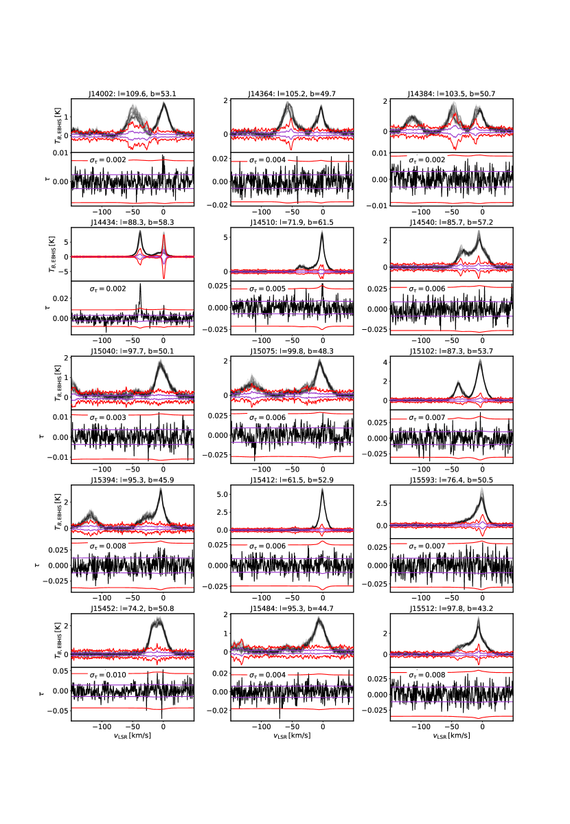
Figure 1: Each panel includes the $21\rm\,cm$ emission ($T_{B}(v)$; upper) from EBHIS (Winkel et al., 2016), and $21\rm\,cm$ optical depth ($\tau_{\rm HI}(v)$; lower) for the $44$ targets in the MACH survey. The median uncertainties in optical depth are printed within each lower panel, and the uncertainties as a function of velocity for $T_{B}(v)$ and $\tau_{\rm HI}(v)$ are overlaid in both panels ($\pm 1\sigma$; purple; $\pm 3\sigma$, red).

Despite the advances of $21\rm\,cm$ absorption studies to date, they are limited by the availability of the brightest background continuum sources for measuring absorption with sufficient sensitivity, and are therefore sparsely distributed. In addition, given the ubiquity of Hi in the Milky Way, the significant blending of $21\rm\,cm$ spectra can make it nearly impossible to distinguish individual Hi structures. Detailed comparisons between real $21\rm\,cm$ observations and synthetic observations of numerical simulations have shown that the completeness of “cloud” recovery declines severely with decreasing Galactic latitude due to crowding of Hi spectral line profiles in velocity (Murray et al., 2017). At high latitudes the line of sight path length through the global cool Hi layer is just a few times the CNM scale height ($h\sim 120\rm\,pc$), providing our best opportunity to reliably measure the properties of individual Hi structures. These properties include the column density, temperature and turbulent Mach number, all of which provide important benchmarks for numerical models of the ISM (e.g., Villagran & Gazol, 2018).

In addition, constraining the properties of Hi at high latitude is important for sorting out the ISM mass budget. It is clear that Hi and carbon monoxide (CO) emission observations are missing significant quantities of gas in galaxies traced by dust and gamma ray emission (e.g., Grenier et al., 2005; Planck Collaboration et al., 2011). This so-called “CO-dark” gas can be accounted for in several ways, including by poorly-shielded H₂ molecules, variations in dust grain emissivity (which controls the conversion between dust emission and mass), or optically-thick Hi (e.g., Reach et al., 2017a, b). Although data from previous Hi absorption studies is sufficient to statistically rule out the hypothesis that optically-thick Hi dominates dark gas (Murray et al., 2018a), quantifying its influence requires building expanded samples which probe diverse Galactic environments.

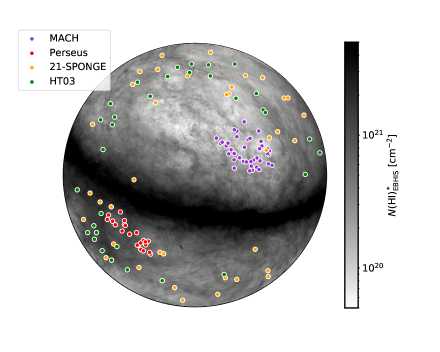
Figure 2: Distribution of MACH target sources (purple) overlaid on a zenith-equal-area (ZEA) map of the Hi column density from EBHIS (Winkel et al., 2016). The target sources comprising the comparison sample from Stanimirović et al. (2014, “Perseus”), Murray et al. (2018b, “21-SPONGE”) and Heiles & Troland (2003a, HT03) are included (red, green and orange circles, respectively).

In this work, we present data from Measuring Absorption by Cold Hydrogen (MACH) – a survey of $21\rm\,cm$ absorption at high Galactic latitude with the Karl G. Jansky Very Large Array (VLA). MACH increases the sample of publicly available, high-sensitivity $21\rm\,cm$ absorption spectra by $50\%$. The paper is organized as follows. In Section 2 we discuss the VLA observations and data reduction strategy, including extraction of matching $21\rm\,cm$ emission. In Section 3, we present our analysis methodology, including computing integrated Hi properties along MACH lines of sight (LOS) and decomposing MACH LOS into individual Hi structures via autonomous Gaussian decomposition. In Section 4, we present the results of our analysis, including a parallel, identical analysis of available high-latitude $21\rm\,cm$ absorption from the literature. In Section 5, we discuss the comparison between MACH and the rest of the high-latitude sky, and estimate the covering fraction of cold Hi. Finally, in Section 6 we summarize the results and present our conclusions.

2 Data

2.1 Observations

For the MACH survey, we targeted extragalactic continuum sources in the region defined by $30<b<62^{\circ}$, $60<l<110^{\circ}$. This region was selected to probe absorption by the local ISM at high latitude, and to overlap with the high-velocity cloud Complex C. We selected the $42$ sources from the VLA-FIRST survey (Becker et al., 1995) with bright flux density at $21\rm\,cm$ ($S_{\rm 21cm}>0.45\rm\,Jy$) and source size estimates $<5^{\prime\prime}\times 5^{\prime\prime}$. These parameters were chosen to maximize sensitivity to absorption and ensure that the majority of our targets would be unresolved.

Observations were conducted at the VLA between August 2017 and February 2018 and spanned several VLA configurations, including C, B, and BnA, as well as configuration moves (C to B, BnA to A). We observed 42 target sources in 51 hours, for an average of $\sim 50$ minutes per target. Each observation utilized three separate, standard L-band configurations, each with one dual-polarization intermediate frequency band of width $1\rm\,MHz$ and $1.95\rm\,kHz$ per channel spacing. The target band was centered on the Hi line ($1.42040575\rm\,GHz$) at a velocity in the local standard of rest (LSR) of $v_{\rm LSR}=-50\rm\,km\,s^{-1}$ and two offline bands were centered at $\pm 1\rm\,MHz$ respectively. The offline bands were used to perform bandpass calibration via frequency switching, as Hi absorption at Galactic velocities in the direction of our calibrator sources can be significant (Murray et al., 2015, 2018b). The absolute phase change associated with frequency switching does not affect our results, as we normalized our solutions with respect to the continuum (see below). Our setup resulted in a velocity coverage of $200\rm\,km\,s^{-1}$ ($-150\rm\,km\,s^{-1}-50\rm\,km\,s^{-1}$) with $0.42\rm\,km\,s^{-1}$ channel spacing, which corresponds to $\sim 0.5\rm\,km\,s^{-1}$ velocity resolution (Rohlfs & Wilson, 2004). We observed nearby VLA calibrator sources for phase and amplitude calibration, and employed self-calibration on each target source for relative flux calibration.

2.2 Data Reduction

Following the strategy of the 21-SPONGE survey, we reduced all MACH data using the Astronomical Image Processing System (AIPS; Greisen, 2003). As a first step, all baselines shorter than $300\rm\,m$ were excluded to avoid contamination from partially-resolved Hi emission. After interactive flagging of noisy baselines, time intervals and antennas using AIPS task TVFLG, we computed an initial bandpass calibration solution for each of the frequency-switched subbands using AIPS task BPASS, and examined them with AIPS task BPLOT to verify good solutions for each antenna. We then combined the offline subbands to create a final bandpass solution to apply to the target.

Turning to the target data set, we performed amplitude and phase calibration with AIPS task CALIB. Next, we determined the relative flux calibration using self-calibration on the target source. This involves isolating the target source continuum, constructing an image using AIPS task IMAGR and using it to calibrate the continuum data set. This process was repeated until the signal to noise in the continuum image following each round of calibration no longer improved significantly (typically requires $1-2$ iterations). Next, we subtracted the continuum from the target by fitting a linear model to line-free channels with AIPS task UVLSF, corrected the target source velocities for Earth’s rotation and LSR motion using AIPS task CVEL, and finally applied the self-calibration solution to the target.

Following flagging and calibration, we constructed final image cubes using IMAGR. We estimated the background noise for each target using a test image of one channel, and cleaned each cube to $3\times$ this level. The pixel size for each cube was computed to be $\sim 4\times$ smaller than the synthesized beam size in order to properly sample the beam.

All target sources were unresolved by our observations, except in two cases: J17104, and J17251. When unresolved, the final spectrum was extracted from the central pixel (i.e., pixel of maximum flux density) of each cleaned data cube. For the two resolved sources, we extracted two spectra each from the two local maxima in flux density. To compute the absorption profile ($\tau_{\rm HI}(v)$), we normalized each extracted spectrum by the flux density at the same pixel in the continuum image.

In Table 1 we list the names, coordinates, flux densities (Becker et al., 1995), and observation details (array configuration, observation date, on-source time) for the MACH targets. The $\tau_{\rm HI}(v)$ spectra are shown in Figure 1, and Figure 2 displays the target locations overlaid on an Hi column density map from the EBHIS survey (Winkel et al., 2016).

2.3 Matching HI Emission

In addition to absorption, measuring the physical properties of neutral ISM structures requires constraints for Hi emission.

Table 1: MACH Observation Information

Name	RA	Dec	$S_{1.4\rm GHz,\,FIRST}$	VLA Config	Date	Time on source	$\sigma_{\tau_{\rm HI}}$
	(∘)	(∘)	(mJy/bm)			(min)
(1)	(2)	(3)	(4)	(5)	(6)	(7)	(8)
J140028+621038	210.118	62.177	4256.2	C	17-Aug-21	20.0	0.002
J143645+633638	219.189	63.610	855.4	C	17-Aug-19	28.6	0.004
J143844+621154	219.685	62.198	2318.6	C	17-Aug-21	20.0	0.002
J144343+503431	220.930	50.575	1181.6	BnA	18-Feb-16	25.4	0.002
J145107+415441	222.780	41.911	792.2	B	18-Jan-14	30.6	0.005
J145408+500331	223.535	50.058	868.2	BnA	18-Feb-01	27.2	0.006
J150409+600055	226.037	60.015	1494.9	C	17-Aug-23	22.2	0.003
J150757+621334	226.987	62.226	511.4	C	17-Aug-18	72.1	0.006
J151020+524430	227.584	52.742	500.5	BnA	18-Feb-01	60.2	0.007
J153948+611356	234.949	61.232	485.1	C	17-Aug-26	74.1	0.008
J154122+382029	235.345	38.341	564.4	B	17-Dec-14	50.1	0.006
J155931+434916	236.285	47.865	739.9	B	18-Jan-07	33.4	0.007
J154525+462244	236.356	46.379	459.0	BnA	18-Feb-07	29.2	0.010
J154840+614731	237.167	61.792	527.6	C, C$\rightarrow$B	17-Aug-26	74.3	0.004
J155128+640537	237.866	64.093	662.9	C	17-Aug-22	68.4	0.008
J160246+524358	240.693	52.733	557.5	B, BnA	18-Jan-28	58.6	0.005
J160427+605055	241.113	60.848	572.2	C	17-Aug-26	64.1	0.008
J161148+404020	242.952	40.672	553.5	B	17-Nov-17	51.0	0.005
J162557+413440	246.490	41.578	1694.6	B	17-Oct-20	22.3	0.003
J163113+434840	247.804	43.811	581.0	B	17-Nov-12	24.5	0.009
J163433+624535	248.638	62.759	4829.3	C	17-Aug-24	13.0	0.001
J163510+584837	248.793	58.810	506.2	C$\rightarrow$B	17-Aug-29	64.1	0.005
J164032+382641	250.133	38.445	464.3	B	18-Jan-27	52.5	0.006
J164258+394837	250.745	39.810	6050.1	B	18-Jan-05	20.2	0.001
J164800+374429	252.000	37.741	625.7	BnA$\rightarrow$A	18-Feb-21	26.1	0.002
J165352+394536	253.467	39.760	1394.4	B	17-Dec-05	24.1	0.004
J165720+570553	254.336	57.098	813.5	BnA	18-Feb-02	30.1	0.002
J165746+480832	254.445	48.142	981.9	B	18-Jan-17	34.3	0.002
J165802+473749	254.511	47.630	873.8	BnA	18-Feb-02	29.3	0.005
J165822+390625	254.592	39.107	646.7	B	18-Jan-11	43.2	0.006
J170246+551639	255.696	55.277	574.3	B	18-Jan-26	59.1	0.003
J170253+501741	255.721	50.295	951.5	B	18-Jan-06	64.8	0.006
J170541+521454	256.422	52.249	504.0	BnA$\rightarrow$A	18-Feb-26	29.3	0.007
J171044+460124	257.683	46.026	643.5	B	17-Dec-11	33.3	0.008
J171044+460124	257.687	46.025	985.0	”	”	”	0.006
J171959+640436	259.997	64.076	817.9	C	17-Aug-26	28.6	0.007
J172339+523648	260.916	52.613	465.4	B	18-Jan-28	58.5	0.010
J172516+403641	261.317	40.611	635.6	B, BnA, BnA$\rightarrow$A	18-Jan-28	87.1	0.004
J172516+403641	261.319	40.612	635.6	”	”	”	0.008
J173044+490626	262.685	49.107	782.2	B	17-Dec-21	37.1	0.005
J173054+381150	262.725	38.197	530.0	B	17-Dec-03	52.6	0.008
J173957+473758	264.988	47.633	907.9	B	18-Jan-19	34.3	0.005
J174036+521143	265.154	52.195	1508.2	B	18-Jan-28	24.2	0.003
J174223+540332	265.598	54.059	450.2	B	17-Nov-25	58.6	0.009

Note. — MACH sources listed in order of RA. (1): Target name; (2, 3): RA and Dec coordinates; (4): Flux density at $21\rm\,cm$ from the VLA-FIRST survey (Becker et al., 1995); (5): VLA array configuration(s) (“$\rightarrow$” denotes configuration move); (6): Observation date; (7) Total time on-source; (8): Achieved. RMS noise in optical depth ($\sigma_{\tau_{\rm HI}}$) per $0.42\rm\,km\,s^{-1}$ channels.

This is not straightforward to acquire, as the presence of the background continuum source precludes us from observing emission from precisely the same structures as we are sensitive to in absorption. Furthermore, obtaining emission observations on the same angular scale as absorption from a facility such as the VLA is prohibitively expensive, as the noise in brightness temperature is proportional to the inverse square of the half power at full width of the telescope beam (Dickey & Lockman, 1990).

A common strategy for estimating the “expected” Hi brightness temperature profile in the absence of background continuum therefore is to observe positions surrounding the target source with lower-resolution single-dish telescopes and interpolate between them. The highest-resolution survey of $21\rm\,cm$ emission to date in the MACH footprint is from the Effelsberg-Bonn Hi Survey (EBHIS; Winkel et al., 2010; Kerp et al., 2011; Winkel et al., 2016). EBHIS is an all-Northern sky (North of Dec$=-5^{\circ}$) survey with high angular resolution ($9^{\prime}$), high sensitivity ($\sigma_{\rm rms}=90\rm\,mK$) and $1.3\rm\,km\,s^{-1}$ per channel velocity resolution.

For each MACH target, we extract all EBHIS spectra within a circle of radius $12^{\prime}$ ($4$ pixels, where each pixel corresponds to $3^{\prime}$), and exclude spectra within a circle corresponding roughly to one EBHIS beam full width at half maximum (FWHM) from the target (radius $1.5$ pixels), which are typically contaminated by the continuum source. Instead of interpolating between the resulting set of $40$ $T_{B}(v)$ spectra, we will use each of these spectra separately as if it were the on-source spectrum, and use the distributions in the resulting fitted parameters to incorporate the significant uncertainty in $T_{B}(v)$ variations to infer Hi physical properties.

2.4 Uncertainty

The brightness temperature of Hi at Galactic velocities can raise the system temperature of a radio receiver, and therefore the uncertainty in $\tau_{\rm HI}(v)$ will vary as a function of velocity. To estimate the uncertainty spectra ($\sigma_{\tau\rm HI}(v)$) we follow the methods outlined in Murray et al. (2015, Section 3.2), which were developed following (Roy et al., 2013). To estimate the uncertainty in the associated brightness temperature ($\sigma_{TB}(v)$), we compute the standard deviation of $T_{B}(v)$ from all $40$ off-positions extracted around each target source. Figure 1 displays the $44$ MACH sightlines, including $\tau_{\rm HI}(v)$, and $T_{B}(v)$ for the $40$ off-positions for each source. In Table 1 we include the median root mean square (rms) uncertainty in optical depth per $0.42\rm\,km\,s^{-1}$ channels for all LOS.

All MACH $\tau_{\rm HI}(v)$ spectra and their associated uncertainties are publicly available.

3 Analysis

3.1 Line of Sight Properties

To estimate the ensemble properties of Hi for the MACH and comparison samples, we integrate $\tau_{\rm HI}(v)$ and $T_{B}(v)$ along the sightline.

The total column density ($N(\rm H\textsc{i})$) is given by,

$$N({\rm HI})=C_{0}\int\tau_{\rm HI}\,T_{s}\,dv,$$ (1)

where $C_{0}=1.823\times 10^{18}\rm\,cm^{-2}/(K\,km\,s^{-1})$ (Draine, 2011) and $T_{s}$ is the Hi excitation temperature, also known as the “spin” temperature. To approximate the spin temperature using observable Hi properties, we assume that Hi a at a single temperature dominates each velocity channel, so that,

$$T_{s}(v)\simeq\frac{T_{B}(v)}{1-e^{-\tau_{\rm HI}(v)}}.$$ (2)

As a result, the $N(\rm H\textsc{i})$ is given by (e.g., Dickey & Benson, 1982),

$$N({\rm HI})\simeq C_{0}\int\frac{\tau_{\rm HI}\,T_{B}}{(1-e^{-\tau_{\rm HI}})}\,dv.$$ (3)

The approximation to $N(\rm H\textsc{i})$ given by Equation 3 has been shown to agree with sophisticated multiphase analysis of $21\rm\,cm$ spectral line pairs (Stanimirović et al., 2014; Murray et al., 2018b). Specifically, in low-column density regimes ($N(\rm H\textsc{i})$$<5\times 10^{20}\rm\,cm^{-2}$), Equation 3 is fully consistent with the results of decomposing $T_{B}(v)$ and $\tau_{\rm HI}(v)$ into individual velocity components of distinct temperature and density and accounting for the order of components along the sightline. In addition, Kim et al. (2014) showed using synthetic $21\rm\,cm$ observations of 3D hydrodynamic simulations of the Galactic ISM that Equation 3 approximates the true simulated column density to within $5\%$. For our high-latitude samples (MACH and comparison, all with $|b|>10^{\circ}$), we will use this approximation for $N(\rm H\textsc{i})$.

If the gas is optically-thin ($\tau_{\rm HI}<<1$), Equation 3 reduces to,

$$N({\rm HI})^{*}=C_{0}\int T_{B}\,dv,$$ (4)

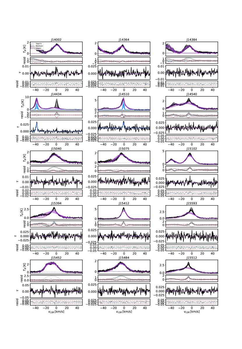
Figure 3: Gaussian fits to MACH LOS using GaussPy. Each panel corresponds to a different sightline, including $T_{B}(v)$ from the $40$ off-positions (top sub-panel), and $\tau_{\rm HI}(v)$ (bottom sub-panel), with the total fits (dotted purple) to $\tau_{\rm HI}(v)$ (Equation 1; Murray et al., 2018b) and $T_{B}(v)$ (Equation 8), the individual components (solid, colors) and the residuals from the fits (sub-panels; grey), along with $\pm 3\sigma$ uncertainties (red).

which is a common assumption used to compute $N(\rm H\textsc{i})$ in the absence of $\tau_{\rm HI}(v)$ measurements. To quantify how much column density is “missed” in the optically-thin limit due to the presence of optically-thick Hi, we compute the ratio of the two column density estimates,

$$\mathcal{R}_{\rm HI}=\frac{N({\rm HI})}{N({\rm HI})^{*}}.$$ (5)

Next, we estimate the relative contribution of cold vs. warm Hi by computing the fraction of the CNM along the line of sight ($f_{\rm CNM}$). We follow the methods outlined by Murray et al. (2020) (their Section 2.5.2; based on Kim et al., 2014), who argue that $f_{\rm CNM}$ is approximated by,

$$f_{\rm CNM}\approx\frac{T_{c}}{\langle T_{s}\rangle}\frac{T_{s,w}-\langle T_{s}\rangle}{T_{s,w}-T_{c}},$$ (6)

where $\langle T_{s}\rangle$ is the optical depth-weighted average spin temperature,

$$\langle T_{s}\rangle=\frac{\int\tau_{\rm HI}\,T_{s}\,dv}{\int\tau_{\rm HI}\,dv},$$ (7)

$T_{c}$ is the kinetic temperature of the CNM and $T_{s,w}$ is the spin temperature of the WNM. Following Murray et al. (2020) we set $T_{c}=50\rm\,K$ and $T_{s,w}=1500\rm\,K$. To account for the considerable uncertainty in these estimates (e.g., the true WNM $T_{s}$ can be much higher than $1500\rm\,K$), we vary these estimates between $20<T_{c}<150\rm\,K$ (Dickey et al., 2000) and $1000<T_{s,w}<6000\rm\,K$ when computing the uncertainties for $f_{\rm CNM}$ (see below). To compute the uncertainties in $N(\rm H\textsc{i})$, $\mathcal{R}_{\rm HI}$ and $f_{\rm CNM}$, we perform a simple Monte Carlo exercise. Over $10^{5}$ trials, we recompute each value after adding random noise to $T_{B}(v)$ and $\tau_{\rm HI}(v)$ drawn from $\pm 3\times\sigma_{TB}(v)$ and $\pm 3\times\sigma_{\tau\rm HI}(v)$ respectively. For $f_{\rm CNM}$, we also vary the values of $T_{c}$ and $T_{s,w}$ as discussed above. We then repeat this computation for each of the $40$ off-positions. The final values and uncertainties for each parameter are computed as the median and standard deviation over all trials.

3.2 Gaussian Decomposition

Beyond integrated properties, we are interested in estimating the properties of individual Hi structures. To decompose the $21\rm\,cm$ spectral line pairs, we follow the methods described by Murray et al. (2018b) for the 21-SPONGE survey (summarized here for clarity), which are based on the strategy employed by Heiles & Troland (2003a, b, ; hereafter HT03).

We begin by decomposing each $\tau_{\rm HI}(v)$ spectrum using the Autonomous Gaussian Decomposition (AGD) algorithm (Lindner et al., 2015), implemented via its open-source Python package GaussPy. AGD provides initial guesses for the number and properties of all Gaussian components (amplitude ($\tau_{0}$), mean velocity ($v_{0}$) and linewidth (FWHM $\delta v$)) within $\tau_{\rm HI}(v)$ by computing successive numerical derivatives with regularization. First, all $21\rm\,cm$ emission/absorption pairs are re-sampled to $0.1\rm\,km\,s^{-1}$ per channel resolution to avoid aliasing narrow components (Lindner et al., 2015). For the fit, we use the “two-phase” implementation of AGD, wherein we identify CNM-like (narrow linewidth) and WNM-like (broad linewidth) components in two steps, using regularization parameters $\alpha_{1}=1.12$ and $\alpha_{2}=2.75$ and a signal-to-noise cutoff of $S/N>3$ for both phases (Murray et al., 2017, 2018b). Given $J$ Gaussian components predicted by AGD for each spectrum, we produce a model for $\tau_{\rm HI}(v)$ using Murray et al. (2018b) Equation 1 via least-squares fit implemented in GaussPy.

The next step is to determine the emitting properties of the fitted absorption components. Specifically, we assume that the $J$ fitted absorption components contribute both optical depth and emission along the line of sight and an additional $K$ components, dominated by WNM, are only detected in emission (e.g., Mebold et al., 1997; Dickey et al., 2000; Murray et al., 2015, HT03). First, we use the Levenberg-Marquart algorithm implemented in the Python package lmfit to perform a least-squares fit of the fitted properties of the $J$ absorption components to $T_{B}(v)$. We allow the amplitudes of the components to vary freely, and constrain their mean velocities to vary with $\pm 2$ channels, and their FWHM to vary by $\pm 10\%$. From the residuals of this initial fit, we use AGD to determine starting guesses for the properties of $K$ additional emission-only components using the one-phase fit ($\alpha=3.75,\,S/N\geq 3$; Murray et al., 2018b). The properties of all $J+K$ components are estimated with an additional least-squares fit to $T_{B}(v)$ (Murray et al., 2018b, Equation 2).

We emphasize that the GaussPy fits are sensitive to the selection of the regularization and other parameters (e.g., signal to noise thresholds, mean velocity and FWHM variation). The systematic uncertainty in the resulting parameters is therefore large, and similar to if we selected the Gaussian fit properties by hand as is traditionally done. The benefit of the GaussPy implementation is that the results are reproducible.

In summary, for each source we have constraints for the properties for the $J$ components fitted to $\tau_{\rm HI}(v)$: including their amplitudes ($\tau_{0,j}$), full widths at half maximum ($\delta v_{0,j}$) and mean velocities ($v_{0,j}$) in absorption. For each of the $40$ off-positions in $T_{B}(v)$, we have constraints for the amplitudes ($T_{0,j}$), FWHMs ($\delta v_{j,\rm em}$) and mean velocities ($v_{0,j,{\rm em}}$) of the $J$ absorption-detected components in emission, as well as the amplitudes ($T_{0,k}$), FWHMs ($\delta v_{k}$) and mean velocities ($v_{0,k}$) of the $K$ additional components fitted only in emission.

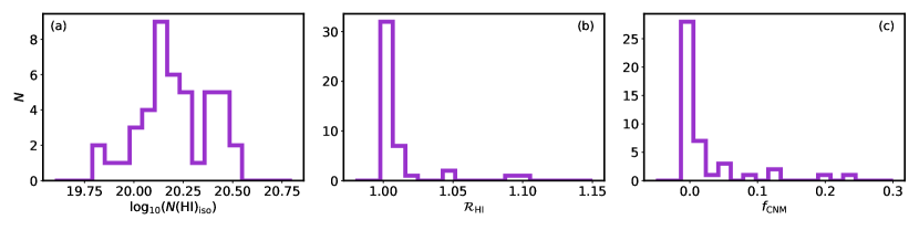
Figure 4: Histograms of integrated properties along MACH LOS, including total Hi column density ($N({\rm HI})$; Equation 3; a), optical depth correction factor ($\mathcal{R}_{\rm HI}$; Equation 5; b) and CNM fraction ($f_{\rm CNM}$; Equation 6; c).

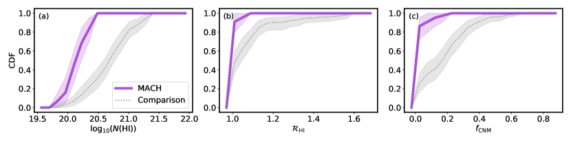
Figure 5: Comparison of cumulative distribution functions (CDFs) of integrated Hi properties between the MACH sample (purple) and the high-latitude comparison sample (grey; Section 3.3), including total Hi column density ($N({\rm HI})$; Equation 3; a), optical depth correction factor ($\mathcal{R}_{\rm HI}$; Equation 5; b) and CNM fraction ($f_{\rm CNM}$; Equation 6; c). The uncertainty ranges in the CDFs are computed by bootstrapping the samples (see text).

3.2.1 Inferring physical properties

Our ultimate goal is to infer important physical properties such as kinetic temperature ($T_{k}$), spin temperature ($T_{s}$), column density ($N(\rm HI)$) and turbulent mach number ($\mathcal{M}_{t}$) using fitted spectral line properties. Following HT03, to this end we need to take into account the order of components along the line of sight ($\mathcal{O}$), as well as the fraction of emission-only components absorbed by foreground absorption components, both of which affect the inferred values of $T_{s}$ (HT03). In detail we solve,

$$T_{B}(v)=T_{B,\rm abs}(v)+T_{B,\rm em}(v),$$ (8)

where $T_{B,\rm abs}(v)$ and $T_{B,\rm em}(v)$ are the contribution of the $J$ absorption-detected components and $K$ emission-only components to $T_{B}(v)$ respectively. These are given by,

$$T_{B,\rm abs}(v)=\sum_{j=0}^{J-1}T_{s,j}(1-e^{-\tau_{j}(v)})e^{-\sum_{m=0}^{M-1}\tau_{m}(v)},$$ (9)

where for each $j^{\rm th}$ component, $\tau_{j}(v)$ is the Gaussian model in absorption and $T_{s,j}$ is the spin temperature, and the subscript $m$ denotes all components lying in front of the $j^{\rm th}$ component along the sightline. The contribution from the $K$ emission-only components is given by,

$$T_{B,\rm em}(v)=\sum_{k=0}^{K-1}[\mathcal{F}_{k}+(1-\mathcal{F}_{k})e^{-\tau(v)}]\,g(T_{k},v_{0,k},\delta v_{k}),$$ (10)

where $\mathcal{F}_{k}$ is the fraction of the $k^{\rm th}$ component which lies in front of the $N$ absorption components and $g(A,v_{0},\delta v)$ is a Gaussian function for amplitude ($A$), mean velocity ($v_{0}$) and FWHM ($\delta v$).

Determining the best-fit values of $\mathcal{O}$ and $\mathcal{F}$ for each component requires iterating over all permutations of possible values. Following HT03, we first make several simplifying assumptions. First, for each of the $K$ emission components, we allow $\mathcal{F}_{k}=(0,0.5,1)$, as finer variations are difficult to distinguish statistically (HT03; Murray et al., 2015; Nguyen et al., 2018). We are then left with $J!\times 3^{K}$ possible combinations of $\mathcal{O}$ and $\mathcal{F}$ for each sightline. However, in practice, the $\mathcal{O}$ only matters for those which overlap significantly, and therefore we only permute the $J_{x}\leq J$ components which overlap with at least one other by at least $3\times\sigma_{\tau}\times\delta v_{j,\rm em}$. In addition, we consider $\mathcal{F}$ only for the $K_{x}\leq K$ emission components which overlap absorption components by at least $3\times\sigma_{T_{B}}\times\delta{v_{k}}$. The result is $J_{x}!\times 3^{K_{x}}$ iterations per sightline. For MACH, the total iterations ranged from 1 to 54, and for the comparison sample (which includes more complex LOS) the total iterations varied from 1 to 19440.

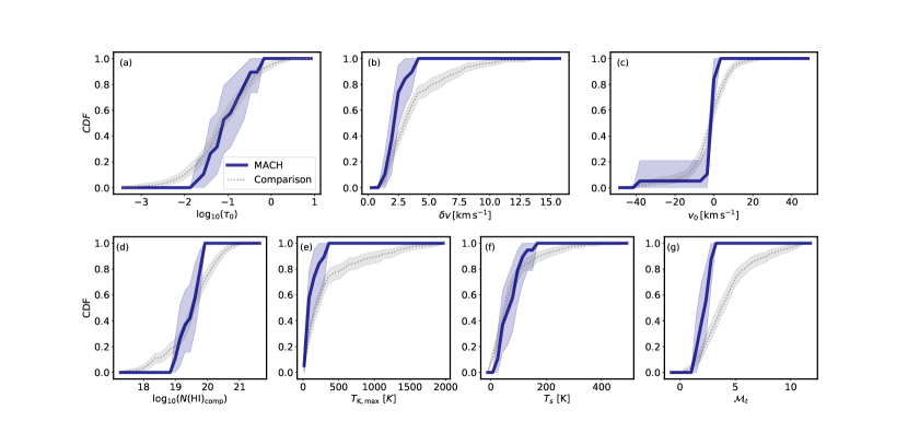
Figure 6: Comparison of cumulative distribution functions (CDFs) of parameters from the Gaussian fits to MACH (dark blue) and the high-latitude comparison sample (grey; Section 3.3), including amplitude ($\tau_{0}$; a), line width (FWHM; $\delta v$; b), mean velocity ($v_{0}$; c), and derived physical properties including column density (Equation 11, $N({\rm HI})_{\rm comp}$; d), maximum kinetic temperature (Equation 12, $T_{\rm K,max}$; e), spin temperature ($T_{s}$; f), and turbulent Mach number (Equation 13, $\mathcal{M}_{t}$; g). The uncertainty ranges in the CDFs are computed by bootstrapping (see text).

3.2.2 Final fits

We repeat this fitting procedure for each of the $40$ $T_{B}(v)$ spectra from the off-positions surrounding each absorption target. In each case, we repeat the permutations of $\mathcal{O}$ and $\mathcal{F}$ described above. For each permutation, we estimate $T_{s,j}$ for the $J$ absorption components by least-squares minimization of the fit to Equation 8.

Next, we follow HT03 and compute a weighted average of $T_{s}$ over all permutations of $\mathcal{O}$ and $\mathcal{F}$, where the weight of each trial is the reciprocal of the variance from the residuals to the fit to $T_{B}(v)$.

In Figure 3, we display the results of the fits for all $40$ off-positions for all MACH LOS. We observe that the fit to $\tau_{\rm HI}(v)$ performed well, and all residuals are within $\pm 3\sigma_{\tau\rm HI}(v)$. We also observe that the overall emission fits exhibit strong residuals. These generally fall within the $\pm 3\sigma_{T_{B}}(v)$ uncertainties, which are considerable due to the strong variation in $T_{B}(v)$ between off positions. In addition, by design, after accounting for detected absorption components the fit to $T_{B}(v)$ is sensitive only to broad, WNM-like components parameterized by a single “one-phase” regularization parameter via AGD. So, not only is the procedure trained against fitting additional, CNM-like narrow components to $T_{B}(v)$, but narrow emission features also correspond to the strongest per-channel uncertainties in $T_{B}(v)$ (Figure 1), making them even less likely to be included. As we are chiefly concerned with the properties of the absorption-detected components, and considering the well-known uncertainties of matching pencil-beam absorption measurements with emission derived from significantly larger angular scales, we accept the increased uncertainties in the emission fits presented here, which will propagate into the uncertainties in the derived parameters.

Overall, following the fits, for each of the $J$ detected absorption components we have $40$ estimates of $T_{s,j}$ and the Gaussian parameters in emission ($T_{0,j}$, $\delta v_{j,\rm em}$, $v_{0,j,{\rm em}}$). The final fitted values for these properties are computed by bootstrapping the $40$ values with replacement over $10^{4}$ trials, and computing the mean of the resulting distribution. The final uncertainties are computed by adding the standard deviation of the bootstrapped distribution (i.e., the uncertainty due to the variation off positions) in quadrature with the mean uncertainty from the least-squares fit to $T_{B}(v)$ over all $40$ positions.

Given $T_{s}$ for each absorption component, we compute the column density per component as,

$$N({\rm HI})_{\rm abs}=C_{0}\int\tau\,T_{s}\,dv=1.064\,C_{0}\,\tau_{0}\,\delta v\,T_{s},$$ (11)

where the factor of $1.064$ converts the product to the area of a Gaussian with the given FWHM and amplitude. We also estimate the maximum kinetic temperature, or the upper limit to the kinetic temperature in the absence of non-thermal broadening, from the absorption line width, via,

$$T_{k,\rm max}=\frac{m_{H}}{8\,k_{B}\ln{2}}\delta v^{2}=21.866\,\delta v^{2}$$ (12)

for hydrogen mass $m_{H}$ and Boltzmann’s constant $k_{B}$ (Draine, 2011). Finally, we compute the turbulent Mach number ($\mathcal{M}_{t}$) via the ratio of $T_{k,\rm max}$ and $T_{s}$. Following HT03 (their Equation 17), we compute,

$$\mathcal{M}_{t}^{2}=4.2\left(\frac{T_{k,\rm max}}{T_{s}}-1\right).$$ (13)

3.3 Comparison Sample

To compare Hi properties along MACH sightlines with other high-latitude environments, we build a sample of measurements from the literature. We select sources from surveys of $\tau_{\rm HI}(v)$ outside of the Galactic Plane ($|b|>10^{\circ}$).

1. VLA (21-SPONGE): The $21\rm\,cm$ Spectral Line Observations of Neutral Gas with the Karl G. Jansky Very Large Array (21-SPONGE; Murray et al., 2015, 2018b) is the highest-sensitivity survey for Galactic $\tau_{\rm HI}(v)$ to date at the VLA. The median root mean square (rms) uncertainty in Hi optical depth is $\sigma_{\tau HI}\lesssim 0.001$ per $0.42\rm\,km\,s^{-1}$ channels. We select the 44 21-SPONGE spectra with $|b|>10^{\circ}$.

2. Arecibo (HT03, Perseus): We include additional spectra from single-dish surveys of $\tau_{\rm HI}(v)$ at the Arecibo Observatory, including the Millennium Arecibo $21\rm\,cm$ Absorption-Line Survey (HT03; Heiles & Troland, 2003b) and a targeted survey of the Perseus molecular cloud and its environment (Stanimirović et al., 2014; Lee et al., 2015, hereafter Perseus). The median optical depth sensitivity of both surveys $\sigma_{\tau\rm HI}\lesssim 0.01$ per $0.18\rm\,km\,s^{-1}$ channels. Although single-dish observations of $\tau_{\rm HI}(v)$ are susceptible to contamination from $21\rm\,cm$ emission within the beam, we find excellent correspondence between these studies and interferometric observations from 21-SPONGE (Murray et al., 2015). We select the 60 $\tau_{\rm HI}(v)$ spectra (22 Perseus, 38 HT03) which are unique relative to 21-SPONGE with $|b|>10^{\circ}$.

Figure 2 includes the locations of the selected targets.

With the comparison sample of $\tau_{\rm HI}(v)$ spectra from 21-SPONGE, Perseus and HT03, we extract Hi emission spectra from $40$ off-positions surrounding each target from EBHIS, and compute corresponding uncertainty spectra ($\sigma_{\tau\rm HI}(v)$ and $\sigma_{TB,\rm exp}(v)$) and integrated properties following the same procedures described above for MACH.

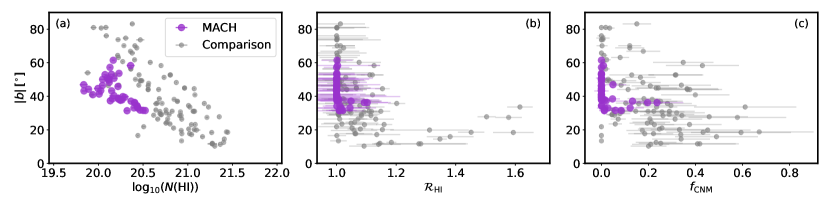
Figure 7: Variation in integrated Hi properties with absolute Galactic latitude ($|b|$) from the MACH sample (purple) and the high-latitude comparison sample (grey), including total Hi column density ($N({\rm HI})$; Equation 3; a), optical depth correction factor ($\mathcal{R}_{\rm HI}$; Equation 5; b) and CNM fraction ($f_{\rm CNM}$; Equation 6; c).

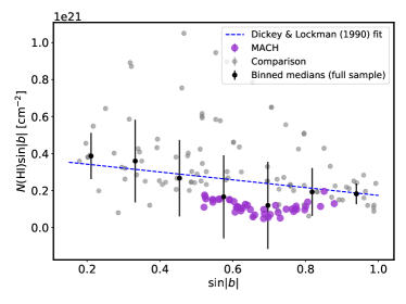
Figure 8: Variation in $N({\rm HI})sin|b|$ with $sin|b|$ for this study (MACH (purple) and comparison (grey) LOS). The binned medians and standard deviations of the both samples together (black) are consistent with previous results (e.g., Dickey & Lockman, 1990), and the MACH LOS trace the minimum column densities, emphasizing the departures of the local ISM from plane-parallel symmetry.

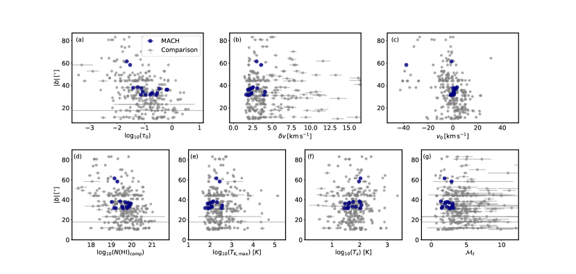
Figure 9: Variation in component Hi properties with absolute Galactic latitude ($|b|$) from MACH (dark blue) and the high-latitude comparison sample (grey), including amplitude ($\tau_{\rm HI}$; a), line width (FWHM; $\delta v$; b), mean velocity ($v_{0}$; c), and derived physical properties including column density (Equation 11, $N({\rm HI})_{\rm comp}$; d), maximum kinetic temperature (Equation 12, $T_{\rm K,max}$; e), spin temperature ($T_{s}$; f), and turbulent Mach number (Equation 13, $\mathcal{M}_{t}$; g).

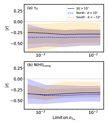
Figure 10: The effect of optical depth sensitivity on correlation with $|b|$. For $\tau_{0}$ (a) and $N({\rm HI})_{\rm comp}$ (b), we plot the $50^{\rm th}$ percentile of the Pearson r coefficient ($|r|$) over $10^{4}$ block-bootstrapped trials in bins of increasing limits to $\sigma_{\tau_{\rm HI}}$, (only components from LOS with $\sigma_{\tau_{\rm HI}}<3\times$ the limit are included), and repeat for the Northern (blue) and Southern (orange) Galactic hemispheres.

In addition, we decompose the comparison sample using the same methodology as for MACH. Given that the comparison sample spectra cover an inhomogeneous range of LSR velocity (e.g., SPONGE absorption spectra cover $-50<v<50\rm\,km\,s$ whereas the Arecibo absorption spectra cover $-100<v<100\rm\,km\,s^{-1}$) we first re-sample the comparison sample spectra to the same velocity axis as MACH spectra (i.e., $-150<v<50\rm\,km\,s^{-1}$ with $0.42\rm\,km\,s^{-1}$ channel spacing). For each spectrum, at velocities where there is no absorption coverage by the original observing setup, we add Gaussian noise with amplitude equal to the median RMS noise in off-line channels. Then, as for the MACH sample, we re-sample again to $0.1\rm\,km\,s^{-1}$ per-channel resolution to ensure that we do not alias narrow velocity components (Lindner et al., 2015). We emphasize that we will restrict our subsequent analysis of fitted component properties to the velocity range common to all spectra ($-50<v<50\rm\,km\,s^{-1}$).

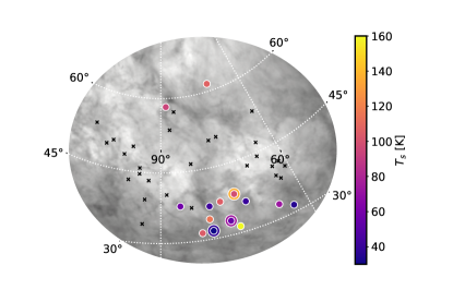
Figure 11: Positions of MACH targets overlaid on $N(\rm H\textsc{i})^{*}$ (HI4PI Collaboration et al., 2016a, ; same scale as Figure 2). Where an absorption component is detected via GaussPy, the point is colored by inferred spin temperature ($T_{s}$). For LOS with multiple components, these are shown as concentric circles. LOS with no detections are shown as black crosses.

To verify if our fitting procedure is consistent with the results of previous analysis of our comparison sample, in Appendix B we compare the distributions of the fitted Gaussian parameters (amplitude, line width, mean velocity) and derived physical properties ($N({\rm HI})_{\rm comp}$, $T_{K,\rm max}$, $T_{s}$, $\mathcal{M}_{t}$) for 21-SPONGE sources with the results of Murray et al. (2018b). We observe in Figure 15 that the results of the original processing of 21-SPONGE spectra are fully consistent with the method presented here within uncertainties. The results of all fits to the comparison sample are displayed in Appendix C.

4 Results

4.1 Properties integrated along LOS

In Figure 4 we display histograms of $N(\rm H\textsc{i})$, $\mathcal{R}_{\rm HI}$, and $f_{\rm CNM}$ for the 44 MACH LOS. Our targets sample a low-column density ($N(\rm H\textsc{i})$$\leq 4\times 10^{20}\rm\,cm^{-2}$), CNM-poor environment (median $\mathcal{R}_{\rm HI}$$=1.0$, median $f_{\rm CNM}$$=0.0$). The maximum column density correction factor that we detect is $\mathcal{R}_{\rm HI}$$=1.10\pm 0.08$ and the maximum CNM fraction is $f_{\rm CNM}$$=0.24\pm 0.11$.

To investigate how the MACH target region compares with other high-latitude environments, we display cumulative distribution functions (CDFs) of $N(\rm H\textsc{i})$, $\mathcal{R}_{\rm HI}$, and $f_{\rm CNM}$ for MACH and the comparison sample in Figure 5. These properties for the $44$ MACH LOS and the comparison sample ($103$ LOS) are also summarized in Appendix A (Table 2). The uncertainty ranges for the CDFs are estimated by bootstrapping each sample with replacement over $10^{4}$ trials, and represent the $1^{\rm st}$ through $99^{\rm th}$ percentiles of limits of the resulting distributions.

Clearly, the MACH sample traces gas with significantly different $N(\rm H\textsc{i})$, $\mathcal{R}_{\rm HI}$, and $f_{\rm CNM}$ than the comparison sample (LOS with $|b|>10^{\circ}$). The MACH CDFs in Figure 5 are fully discrepant within $\pm 3\sigma$ from the comparison sample.

4.2 Properties of individual Hi structures

Given that the integrated properties of MACH LOS are significantly different than the comparison sample, we investigate how the properties of individual Hi structures inferred from the Gaussian fitting procedure (Section 3.2) compare. In Figure 6, we display CDFs of the fitted Gaussian parameters (amplitude, line width, mean velocity) and derived physical properties ($N({\rm HI})_{\rm comp}$, $T_{K,\rm max}$, $T_{s}$, $\mathcal{M}_{t}$) for all components detected along MACH and comparison sample LOS. As in Figure 5, the uncertainty ranges for the CDFs are estimated by bootstrapping the samples, and represent the $1^{\rm st}$ through $99^{\rm th}$ percentiles of each distribution.

From Figure 6, we observe that the amplitudes of Gaussian-fitted components (panel a) are statistically indistinguishable within uncertainties between the MACH and comparison samples. For the component line widths (FWHM; panel b), MACH features statistically more LOS with $\delta v<2.5\rm\,km\,s^{-1}$. In addition, the MACH LOS are dominated by components with mean velocities (panel c) $v_{0}<0\rm\,km\,s^{-1}$ relative to the comparison LOS.

The structures along MACH LOS sample a narrower range of $N({\rm HI})_{\rm comp}$ (Equation 11; panel d) than the comparison sample. The prevalence of low-$\delta v$ components results in smaller $T_{K,\rm max}$ (Equation 12; panel e) for MACH relative to the comparison sample in Figure 6. We observe that the spin temperature distributions (panel f) are statistically similar for low-$T_{s}$: for example, below the maximum $T_{s}$ for MACH ($T_{s}=163\pm 6\rm\,K$) the samples are statistically indistinguishable within uncertainties, however, an additional $\sim 15\%$ of the comparison sample components have $T_{s}>170\rm\,K$. Given the narrower widths and smaller maximum kinetic temperatures, the $\mathcal{M}_{t}$ for MACH structures (Equation 13) is statistically smaller than for the comparison sample structures (panel g).

4.3 Latitude dependence of Hi properties

To further investigate how the MACH environment compares with the rest of the high-latitude sky, we test how the integrated properties and fitted component properties vary with Galactic environment, parameterized by Galactic latitude.

In Figure 7 we plot $N(\rm H\textsc{i})$, $\mathcal{R}_{\rm HI}$, and $f_{\rm CNM}$ for the MACH and comparison samples as a function of absolute latitude ($|b|$). We observe that there is a clear correlation between $N(\rm H\textsc{i})$ and $|b|$ (panel a), where higher latitudes have lower $N(\rm H\textsc{i})$. The MACH sample occupies the lower-$N(\rm H\textsc{i})$ end of the trend, but follows the same trend as the comparison sample. As $|b|$ decreases, each emission/absorption measurement samples a longer path length through the Milky Way, and therefore the resulting $N(\rm H\textsc{i})$ will sample more Hi structures and tend to be larger. In Figure 8, we plot $N({\rm HI})\sin|b|$ vs. $\sin|b|$ for the MACH and comparison LOS, finding fully consistent results with previous analysis ($N({\rm HI})=3.84\times 10^{20}csc|b|$ Heiles, 1976; Dickey & Lockman, 1990). The variation in $N({\rm HI})\sin|b|$ with latitude arises because Hi is not organized in plane-parallel layers (Knapp, 1975; Dickey & Lockman, 1990). The MACH LOS sample the minimum column densities, as a result of the structure of the local ISM, which we will discuss further in Section 5.

In panels (b) and (c) of Figure 7 we observe a very mild trend in $\mathcal{R}_{\rm HI}$ and $f_{\rm CNM}$ with $|b|$ (Pearson r correlation coefficients $-0.40$ and $-0.44$ respectively for the MACH and comparison samples combined). We observe that the largest values of $\mathcal{R}_{\rm HI}$ and $f_{\rm CNM}$ are all at the lowest $|b|$ where the LOS sample the longest path lengths.

In Figure 9, we plot the fitted properties of individual Hi structures as a function of $|b|$ (same quantities as Figure 6). To check for the presence of a correlation, we compute the Pearson r correlation coefficient for the full samples (MACH plus comparison) over $10^{4}$ trials, resampling in each trial. Here we use block bootstrapping, which involves breaking the sky into 10 equally-spaced bins (“blocks”) in both longitude and latitude and resampling these blocks with replacement to incorporate the influence of large-scale interstellar structures into the parameter uncertainty.

In all cases except $\tau_{0}$, $v_{0}$, and $N({\rm HI})_{\rm comp}$ the resulting Pearson r coefficient distributions are consistent with zero, indicating no significant correlation with $|b|$. For $\tau_{0}$, $v_{0}$, and $N({\rm HI})_{\rm comp}$, we observe negative correlation with $|b|$, significant at $>3\sigma$ (in terms of the block-bootstrapped distributions of the Pearson r coefficient).

The negative correlation between $v_{0}$ and $|b|$ arises because of the large-scale Hi distribution. For example, there are many well-known intermediate-velocity clouds (IVCs) in the Northern hemisphere, including the IV Arch and Spur (Kuntz & Danly, 1996) which skew the distribution of $v_{0}$ to negative velocities. We find that the majority of CNM components have central velocities $|v_{0}|<20\rm\,km\,s^{-1}$.

To test for the effects of optical depth sensitivity on the correlation of $\tau_{0}$ and $N({\rm HI})_{\rm comp}$ with $|b|$, we repeat the correlation coefficient estimation for components binned by the RMS noise in the $\tau_{\rm HI}(v)$ spectrum they were fitted to ($\sigma_{\tau_{\rm HI}}$). In Figure 10 we plot the $50^{\rm th}$ percentile of the Pearson r coefficient ($|r|$) as a function of the maximum $3\sigma_{\tau_{\rm HI}}$ limit (i.e., for each bin, only components with $\sigma_{\tau_{\rm HI}}<3\times$ the indicated limit are included). We also split the samples between the Northern and Southern hemispheres. For both $\tau_{0}$ and $N({\rm HI})_{\rm comp}$, the negative correlation with $|b|$ persists across all sensitivity limits within block-bootstrapped uncertainties, for the full, Northern and Southern samples.

The negative correlation between $\tau_{0}$ and $|b|$ in Figure 9 (i.e., higher optical depths at lower latitudes) likely arises due to crowding effects. At lower latitudes where the spectral line complexity is higher, the completeness of Gaussian decomposition for recovering real individual Hi structures declines (Murray et al., 2017). As a result, spectral features which are caused by multiple, blended, low-$\tau_{0}$ components may be incorrectly fit by fewer, higher-$\tau_{0}$ components. We selected our sample to have $|b|>10^{\circ}$ to reduce this bias, but it is still present. The correlation in $\tau_{0}$ propagates to drive the observed correlation with $N({\rm HI})_{\rm comp}$.

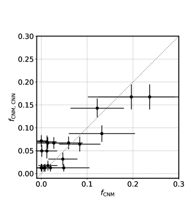
Figure 12: Comparing predictions of $f_{\rm CNM}$ from a convolutional neural network ($f_{\rm CNM}$_,CNN) applied to EBHIS with constraints from MACH ($f_{\rm CNM}$). Within uncertainties, the $f_{\rm CNM}$ and $f_{\rm CNM}$_,CNN are consistent.

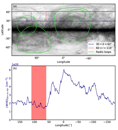
Figure 13: (a): All-sky $N({\rm HI})^{*}$ map (HI4PI Collaboration et al., 2016b, ; same scale as Figure 2) with latitude (red, vertical) and longitude (blue, horizontal) ranges for the MACH survey overlaid, including the outlines of known radio loops (Berkhuijsen et al., 1971). (b): Mean $N({\rm HI})^{*}$ from $30<b<62^{\circ}$ as a function of longitude. The MACH survey (shaded red) covers the minimum column density for this latitude range.

5 Discussion

Overall, we observe that the MACH sample probes a region with significantly low $N(\rm HI)$ and small $f_{\rm CNM}$ relative to the rest of the high and intermediate-latitude sky traced by previous Hi absorption surveys (Figure 5). Although the properties of individual structures are generally similar as those detected across $|b|>10^{\circ}$ (Figure 6), MACH LOS feature Hi structures with smaller $\delta v$, $T_{\rm K,max}$ and $\mathcal{M}_{t}$. These results were not expected when the survey was conceived, and below we discuss the implications.

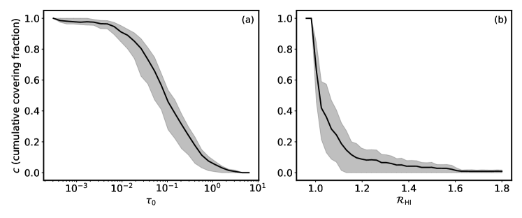
Figure 14: Cumulative sky covering fractions as a function of $\tau_{\rm HI}$ (a) and $\mathcal{R}_{\rm HI}$ (b) from the combined MACH and comparison samples. For (a), for each value of $\tau_{0}$, only sightlines with $\sigma_{\tau_{\rm HI}}\leq 3\times\tau_{0}$ are included in the calculation. The uncertainties (shading) represent the $16^{\rm th}$ through $84^{\rm th}$ percentiles and are computed by block bootstrapping (see text).

That such a large region of the Northern sky could be so low-column and free of CNM is a reflection of how the local Hi distribution departs significantly from pure plane-parallel symmetry. It is well-known that the sun sits in a “Local Bubble” or cavity, full of low-density gas (Cox & Reynolds, 1987), surrounded by other bubble structures believed to be caused by star formation activity (e.g., Berkhuijsen et al., 1971). The MACH field sits in a location where the bubble appears to be breaking out of the disk in a patchy, chimney-like structure (Lallement et al., 2003; Vergely et al., 2010), and the distance to the cool, absorbing Hi along MACH LOS is likely $150$ to $400\rm\,pc$, possibly as close as the edge of the bubble (Lallement et al., 2019).

In Figure 11 we zoom-in on the MACH target region, and plot the LOS by their component $T_{s}$ estimates, with crosses for non-detections. This illustration emphasizes the patchy nature of the CNM distribution at high latitude – for a roughly 400-square degree patch of sky ($60\lesssim l\lesssim 100^{\circ}$, $40\lesssim b\lesssim 50$) we detect no CNM at our optical depth sensitivity limit of $\sim 0.005$ per $0.42\rm\,km\,s^{-1}$ channels, and most detections are clustered together at the lowest latitudes.

Could we have predicted that the MACH region would end up being so low-column and CNM-poor? To address this, we return to an inspection of Figure 1, where we observe that the structure of Hi emission on small scales near MACH LOS provides a reasonable prediction for the presence or absence of absorption lines. Channels featuring the strongest variation in $T_{B}(v)$ between off positions (quantified by $\sigma_{T_{B}}(v)$) tend to correspond with channels of detected absorption at our sensitivity (Dempsey et al., 2020). This is not always the case – for example, for source J14434 we detect absorption associated with only one of two narrow Hi emission features, which reflects the small-scale structure of the CNM in this region. In general, absorption features correspond with the narrowest velocity structures in $T_{B}(v)$, and LOS without detected absorption are free of discernible narrow velocity structure in $T_{B}(v)$. In agreement, Murray et al. (2020) recently showed that a simple convolutional neural network (CNN) trained using synthetic Hi observations can predict $f_{\rm CNM}$ from the velocity structure of $T_{B}(v)$ alone (i.e., without $\tau_{\rm HI}(v)$ information). We applied their CNN model to MACH LOS and compare the resulting estimates ($f_{\rm CNM}$_,CNN) with the constraints from absorption in Figure 12. Within uncertainties, the simple CNN accurately recovers the observed $f_{\rm CNM}$ values. In future studies, this or similar methods may be used to predict where Hi absorption is likely to be detected.

To investigate the state of the MACH region relative to similar high-latitude regions, we plot an all-sky Hi column density ($N({\rm HI})^{*}$) map in Figure 13a, highlighting the MACH latitude and longitude ranges. In Figure 13b we plot the mean $N({\rm HI})^{*}$ across MACH latitudes as a function of longitude, and observe that the MACH region has the lowest $N({\rm HI})^{*}$ for this latitude range. The high-latitude sky is populated by well-known loop structures (overlaid on Figure 13a), which likely trace shocked, swept-up magnetic fields and relativistic electrons, as well as swept-up Hi in fibrous structures from recent supernova activity (Berkhuijsen et al., 1971).

That the morphology of the MACH region appears different (Figure 11) from the swept-up shock picture suggests that the MACH region may not have been hit by a supernova shock recently. This scenario would be consistent with the finding in Figure 9 that CNM components detected along MACH LOS have significantly smaller turbulent MACH number (panel g) than the rest of the high and intermediate-latitude sky. In the relative absence of non-thermal motions from turbulence driven by star formation activity, the CNM line widths will be dominated by thermal motions alone, and $T_{k,\rm max}\approx T_{s}$. So, the MACH LOS may simply be tracing a particularly quiescent, undisturbed patch of sky.

5.1 The covering fraction of cold Hi

Given the patchy nature of the CNM at high Galactic latitudes, we use the assembled sample of absorption constraints (the MACH and comparison samples combined) to estimate the covering fraction of cold Hi.

In Figure 14 we plot the cumulative covering fraction of cold Hi as a function of component optical depth ($\tau_{0}$; a) and column density correction factor ($\mathcal{R}_{\rm HI}$). The covering fractions, $c$ are computed as the fraction of all LOS featuring a component with optical depth greater than or equal to the indicated value (a), or a correction factor greater than or equal to the indicated value (b). In the case of $\tau_{0}$, we take into account the effects of varying optical depth sensitivity between LOS by only considering LOS with $\sigma_{\tau_{\rm HI}}\leq 3\tau_{0}$ for each bin. The uncertainties on the covering fractions are estimated by block-bootstrapping the samples, as discussed previously. We observe from Figure 14a that for Hi structures with $\tau_{0}>0.001$ $c\sim 100\%$: at our sensitivity and within uncertainties, we cannot rule out the presence of this population of components along all LOS. For $\tau_{0}>0.01$, and $\tau_{0}>0.1$, $c\sim 90\%$ and $c\sim 45\%$ respectively. By $\tau_{0}>1$, $c$ consistent with zero, suggesting that individual structures with $\tau_{0}>1$ are not present at high Galactic latitude ($|b|>10^{\circ}$).

A consistent story is presented in Figure 14b. We observe that for LOS with $\mathcal{R}_{\rm HI}$$\geq 1.003$, $c=65\%$, and for $\mathcal{R}_{\rm HI}$$\geq 1.2$ it is only $\sim 10\%$. This further emphasizes the picture that the CNM at high Galactic latitude does not contribute significantly to the total Hi column density. As concluded by Murray et al. (2018a) using a similar comparison sample from the literature, the lack of large Hi optical depths detected in absorption rules out the hypothesis that cold Hi is the dominant form of “dark gas” at high latitude.

However, despite the generally small optical depth of the CNM at high latitude, it is still a dynamically and physically-relevant phase in the ISM energy budget in this environment. Linear Hi structures (or fibers) observed in Hi emission which trace the local magnetic field (Clark et al., 2014, 2015) are dominated by the cold Hi (Clark et al., 2019; Peek & Clark, 2019). In addition, the correlation between Hi and dust emission varies with Hi column density (Lenz et al., 2017; Nguyen et al., 2018), even within the low-column density environment probed here (Murray et al., 2020), indicating that Hi phase balance influences the mixture between gas and dust – critical for precise Galactic foreground estimation.

6 Summary and Conclusions

We have presented the results of MACH, a survey of $21\rm\,cm$ absorption in a high-Galactic latitude patch of sky ($60<l<110^{\circ}$, $30<b<62^{\circ}$) with the VLA. We reach sufficient sensitivity in optical depth to detect absorption by the CNM in this region. For all $44$ LOS, we compute the total column density, fraction of CNM, and the column density correction due to optical depth, as well as the properties of individual Hi structures along each sightline via autonomous Gaussian decomposition. To compare the MACH region with the rest of the high and intermediate latitude sky ($|b|>10^{\circ}$), we analyze a sample of $103$ LOS from the literature and compare the results. Our main results are summarized as follows:

1. The integrated MACH LOS reveal surprisingly low-column density, low-$f_{\rm CNM}$, low-$\mathcal{R}_{\rm HI}$ gas. We find median $N(\rm H\textsc{i})$$=1.5\times 10^{20}\rm\,cm^{-2}$, $f_{\rm CNM}$$=0.0$, $\mathcal{R}_{\rm HI}$$=1.0$ (Figure 4). Relative to the high- and intermediate-latitude sky probed by the comparison sample, these properties are significantly different (Figure 5).

2. Individual Hi structures along MACH LOS have generally similar properties to those detected along comparison sample LOS (Figure 6). However, the line widths, kinetic temperatures and turbulent Mach numbers of MACH structures tend to be smaller. Although star formation activity has disrupted the local Hi structure in the high-latitude sky, producing a patchy distribution of CNM, the MACH LOS may be sampling a particularly low-column, quiescent region undisturbed recently by supernova shocks, leading its Hi properties to be dominated by thermal motions rather than non-thermal, turbulent motions.

3. For the full sample (MACH and comparison combined) we compute the cumulative covering fraction of CNM properties at $|b|>10^{\circ}$ (Figure 14), and find that the high- and intermediate-latitude sky is dominated by gas with small optical depth and column density. For Hi structures with amplitude in optical depth of $\tau_{0}>0.001$, the covering fraction is consistent with $100\%$, For $\tau_{0}>0.01$, $\tau_{0}>0.1$ and $\tau_{0}>1$, the covering fractions are $c=90\%$, $45\%$ and $0\%$ respectively. In terms of the cumulative correction for optical depth ($\mathcal{R}_{\rm HI}$), for $\mathcal{R}_{\rm HI}$$\geq 1.003$ the covering fraction is $c=65\%$ and $\mathcal{R}_{\rm HI}$$\geq 1.2$ it is only $10\%$.

Overall, the MACH LOS demonstrate the power of targeted $21\rm\,cm$ absorption studies to reveal unique interstellar environments in the local ISM. Future, expanded samples of Galactic absorption with similarly high optical depth sensitivity covering significantly larger fractions of sky are incoming with next-generation survey telescopes, including the Australian Square Kilometer Array Pathfinder (Dickey et al., 2013). These samples will enable precise characterization of the CNM properties throughout the Milky Way.

In the meantime, as future work we look forward to tackling additional science goals with the available samples. For example, the relative lack of blended, overlapping lines along MACH LOS make it a powerful sample for constraining the number of absorption lines as a function of optical depth, a calculation typically confounded by the masking of strong absorption lines. In addition, the MACH non-detection LOS provide lower limits to the spin temperature of gas without detected absorption, and can also impose limits on the minimum brightness temperature required for detecting absorption. Finally, we can compare predictions from 3D models of the local dust distribution based on IR emission, stellar photometry, and/or gamma rays (e.g., Remy et al., 2017; Green et al., 2019; Lallement et al., 2019; Leike et al., 2020) with CNM inferred from $21\rm\,cm$ absorption to see if they predict consistent ISM structures in the $\sim 100-500\rm\,pc$ distance regime.

Appendix A Integrated Properties

In the following Appendix, we include a table of integrated properties for the MACH and comparison samples (Table 2).

Table 2: Integrated Properties

Name	Survey	l	b	$N({\rm HI})_{\rm thin}$	$N({\rm HI})$	$\mathcal{R}_{\rm HI}$	$f_{\rm CNM}$
		(∘)	(∘)	($10^{20}\rm\,cm^{-2}$)	($10^{20}\rm\,cm^{-2}$)
(1)	(2)	(3)	(4)	(5)	(6)	(7)	(8)
J14002	MACH	109.589	53.127	1.40$\,\pm\,$0.11	1.40$\,\pm\,$0.11	1.00$\,\pm\,$0.11	0.00$\,\pm\,$0.00
J14364	MACH	105.174	49.730	1.30$\,\pm\,$0.08	1.30$\,\pm\,$0.08	1.00$\,\pm\,$0.09	0.00$\,\pm\,$0.00
J14384	MACH	103.524	50.695	1.50$\,\pm\,$0.13	1.50$\,\pm\,$0.13	1.00$\,\pm\,$0.12	0.00$\,\pm\,$0.00
J14434	MACH	88.257	58.314	2.29$\,\pm\,$0.23	2.29$\,\pm\,$0.23	1.00$\,\pm\,$0.14	0.01$\,\pm\,$0.02
J14510	MACH	71.913	61.477	1.46$\,\pm\,$0.05	1.47$\,\pm\,$0.05	1.00$\,\pm\,$0.05	0.00$\,\pm\,$0.01
J14540	MACH	85.672	57.249	1.35$\,\pm\,$0.04	1.35$\,\pm\,$0.04	1.00$\,\pm\,$0.04	0.00$\,\pm\,$0.00
J15040	MACH	97.691	50.106	1.11$\,\pm\,$0.09	1.11$\,\pm\,$0.09	1.00$\,\pm\,$0.11	0.00$\,\pm\,$0.00
J15075	MACH	99.785	48.310	1.32$\,\pm\,$0.09	1.32$\,\pm\,$0.09	1.00$\,\pm\,$0.10	0.00$\,\pm\,$0.00
J15102	MACH	87.319	53.685	1.70$\,\pm\,$0.07	1.70$\,\pm\,$0.07	1.00$\,\pm\,$0.06	0.00$\,\pm\,$0.00
J15394	MACH	95.340	45.854	1.66$\,\pm\,$0.11	1.66$\,\pm\,$0.11	1.00$\,\pm\,$0.09	0.00$\,\pm\,$0.00
J15412	MACH	61.493	52.905	1.18$\,\pm\,$0.05	1.19$\,\pm\,$0.05	1.00$\,\pm\,$0.06	0.00$\,\pm\,$0.01
J15593	MACH	76.443	50.514	1.32$\,\pm\,$0.07	1.32$\,\pm\,$0.07	1.00$\,\pm\,$0.07	0.00$\,\pm\,$0.01
J15452	MACH	74.158	50.850	1.25$\,\pm\,$0.05	1.26$\,\pm\,$0.05	1.00$\,\pm\,$0.06	0.00$\,\pm\,$0.02
J15484	MACH	95.276	44.657	0.99$\,\pm\,$0.10	0.99$\,\pm\,$0.10	1.00$\,\pm\,$0.15	0.00$\,\pm\,$0.00
J15512	MACH	97.835	43.242	1.41$\,\pm\,$0.09	1.41$\,\pm\,$0.09	1.00$\,\pm\,$0.09	0.00$\,\pm\,$0.01
J16024	MACH	82.293	46.439	1.11$\,\pm\,$0.06	1.11$\,\pm\,$0.06	1.00$\,\pm\,$0.07	0.00$\,\pm\,$0.02
J16042	MACH	92.926	43.385	1.06$\,\pm\,$0.04	1.06$\,\pm\,$0.04	1.00$\,\pm\,$0.06	0.00$\,\pm\,$0.01
J16114	MACH	64.549	46.906	0.68$\,\pm\,$0.07	0.69$\,\pm\,$0.07	1.00$\,\pm\,$0.15	0.05$\,\pm\,$0.06
J16255	MACH	65.744	44.219	0.78$\,\pm\,$0.04	0.78$\,\pm\,$0.04	1.00$\,\pm\,$0.08	0.00$\,\pm\,$0.00
J16311	MACH	68.801	43.200	0.69$\,\pm\,$0.04	0.69$\,\pm\,$0.04	1.00$\,\pm\,$0.07	0.00$\,\pm\,$0.03
J16343	MACH	93.611	39.384	1.97$\,\pm\,$0.11	1.97$\,\pm\,$0.11	1.00$\,\pm\,$0.08	0.00$\,\pm\,$0.00
J16351	MACH	88.639	40.410	1.49$\,\pm\,$0.18	1.49$\,\pm\,$0.18	1.00$\,\pm\,$0.17	0.00$\,\pm\,$0.01
J16403	MACH	61.602	41.327	1.02$\,\pm\,$0.07	1.02$\,\pm\,$0.07	1.00$\,\pm\,$0.10	0.00$\,\pm\,$0.00
3C345	MACH	63.455	40.949	0.87$\,\pm\,$0.04	0.87$\,\pm\,$0.04	1.00$\,\pm\,$0.07	0.00$\,\pm\,$0.00
J16480	MACH	60.857	39.799	1.88$\,\pm\,$0.28	1.88$\,\pm\,$0.28	1.00$\,\pm\,$0.21	0.00$\,\pm\,$0.00
J16535	MACH	63.600	38.859	1.67$\,\pm\,$0.11	1.67$\,\pm\,$0.11	1.00$\,\pm\,$0.09	0.00$\,\pm\,$0.00
J16572	MACH	85.740	37.857	1.83$\,\pm\,$0.18	1.84$\,\pm\,$0.18	1.00$\,\pm\,$0.14	0.01$\,\pm\,$0.02
J16574	MACH	74.368	38.478	1.43$\,\pm\,$0.07	1.44$\,\pm\,$0.07	1.00$\,\pm\,$0.07	0.01$\,\pm\,$0.02
J16580	MACH	73.714	38.439	1.66$\,\pm\,$0.04	1.67$\,\pm\,$0.04	1.01$\,\pm\,$0.03	0.05$\,\pm\,$0.03
J16582	MACH	62.883	37.929	1.73$\,\pm\,$0.09	1.73$\,\pm\,$0.09	1.00$\,\pm\,$0.08	0.00$\,\pm\,$0.01
J17024	MACH	83.347	37.317	1.36$\,\pm\,$0.06	1.36$\,\pm\,$0.06	1.00$\,\pm\,$0.06	0.02$\,\pm\,$0.03
J17025	MACH	77.079	37.600	1.76$\,\pm\,$0.14	1.77$\,\pm\,$0.14	1.01$\,\pm\,$0.11	0.00$\,\pm\,$0.02
J17054	MACH	79.516	37.094	2.21$\,\pm\,$0.16	2.32$\,\pm\,$0.17	1.05$\,\pm\,$0.10	0.13$\,\pm\,$0.07
J17104A	MACH	71.763	36.230	2.31$\,\pm\,$0.13	2.55$\,\pm\,$0.14	1.10$\,\pm\,$0.08	0.24$\,\pm\,$0.11
J17104B	MACH	71.763	36.227	2.31$\,\pm\,$0.13	2.53$\,\pm\,$0.14	1.09$\,\pm\,$0.08	0.20$\,\pm\,$0.09
J17195	MACH	93.806	34.144	2.70$\,\pm\,$0.09	2.70$\,\pm\,$0.09	1.00$\,\pm\,$0.05	0.00$\,\pm\,$0.01
J17233	MACH	79.919	34.350	2.68$\,\pm\,$0.09	2.71$\,\pm\,$0.09	1.01$\,\pm\,$0.05	0.00$\,\pm\,$0.01
J17251B	MACH	65.568	33.018	2.73$\,\pm\,$0.18	2.77$\,\pm\,$0.18	1.02$\,\pm\,$0.09	0.03$\,\pm\,$0.03
J17251A	MACH	65.569	33.016	2.73$\,\pm\,$0.18	2.76$\,\pm\,$0.18	1.01$\,\pm\,$0.09	0.01$\,\pm\,$0.03
J17304	MACH	75.772	33.068	2.39$\,\pm\,$0.15	2.50$\,\pm\,$0.15	1.04$\,\pm\,$0.09	0.12$\,\pm\,$0.06
J17305	MACH	62.989	31.515	3.28$\,\pm\,$0.11	3.34$\,\pm\,$0.11	1.02$\,\pm\,$0.05	0.08$\,\pm\,$0.05
J17395	MACH	74.222	31.396	2.08$\,\pm\,$0.12	2.10$\,\pm\,$0.12	1.01$\,\pm\,$0.08	0.01$\,\pm\,$0.02
J17403	MACH	79.563	31.748	2.89$\,\pm\,$0.07	2.93$\,\pm\,$0.07	1.02$\,\pm\,$0.03	0.01$\,\pm\,$0.02
J17422	MACH	81.770	31.613	3.12$\,\pm\,$0.10	3.16$\,\pm\,$0.10	1.01$\,\pm\,$0.05	0.06$\,\pm\,$0.03
3C327.1A	21-SPONGE	12.181	37.006	6.98$\,\pm\,$0.24	7.67$\,\pm\,$0.28	1.10$\,\pm\,$0.05	0.25$\,\pm\,$0.09
4C16.09	21-SPONGE	166.636	-33.596	9.55$\,\pm\,$0.36	10.56$\,\pm\,$0.43	1.11$\,\pm\,$0.06	0.23$\,\pm\,$0.09
1055+018	21-SPONGE	251.511	52.774	2.85$\,\pm\,$0.09	2.85$\,\pm\,$0.09	1.00$\,\pm\,$0.05	0.00$\,\pm\,$0.01
3C459	21-SPONGE	83.040	-51.285	5.27$\,\pm\,$0.13	5.43$\,\pm\,$0.14	1.03$\,\pm\,$0.04	0.17$\,\pm\,$0.06
3C018A	21-SPONGE	118.623	-52.732	5.72$\,\pm\,$0.15	6.41$\,\pm\,$0.18	1.12$\,\pm\,$0.04	0.32$\,\pm\,$0.12
PKS2127	21-SPONGE	58.652	-31.815	4.31$\,\pm\,$0.21	4.40$\,\pm\,$0.22	1.02$\,\pm\,$0.07	0.09$\,\pm\,$0.04
3C286	21-SPONGE	56.524	80.675	1.07$\,\pm\,$0.04	1.07$\,\pm\,$0.04	1.00$\,\pm\,$0.06	0.03$\,\pm\,$0.02
3C298	21-SPONGE	352.160	60.666	1.87$\,\pm\,$0.04	1.87$\,\pm\,$0.04	1.00$\,\pm\,$0.03	0.01$\,\pm\,$0.01
3C245B	21-SPONGE	233.123	56.299	2.30$\,\pm\,$0.08	2.31$\,\pm\,$0.08	1.00$\,\pm\,$0.05	0.02$\,\pm\,$0.02
3C123B	21-SPONGE	170.578	-11.659	14.69$\,\pm\,$1.46	18.75$\,\pm\,$2.20	1.28$\,\pm\,$0.16	0.41$\,\pm\,$0.16
3C454.3	21-SPONGE	86.112	-38.185	6.85$\,\pm\,$0.33	7.03$\,\pm\,$0.33	1.03$\,\pm\,$0.07	0.22$\,\pm\,$0.08
3C225B	21-SPONGE	220.011	44.009	3.48$\,\pm\,$0.17	3.60$\,\pm\,$0.16	1.03$\,\pm\,$0.07	0.38$\,\pm\,$0.14
3C273	21-SPONGE	289.945	64.359	1.64$\,\pm\,$0.09	1.64$\,\pm\,$0.09	1.00$\,\pm\,$0.08	0.01$\,\pm\,$0.01
UGC09799	21-SPONGE	9.417	50.120	2.58$\,\pm\,$0.10	2.59$\,\pm\,$0.10	1.01$\,\pm\,$0.05	0.03$\,\pm\,$0.02
3C041B	21-SPONGE	131.374	-29.070	5.01$\,\pm\,$0.12	5.05$\,\pm\,$0.12	1.01$\,\pm\,$0.03	0.04$\,\pm\,$0.02
J2232	21-SPONGE	77.438	-38.582	4.71$\,\pm\,$0.24	4.81$\,\pm\,$0.25	1.02$\,\pm\,$0.07	0.18$\,\pm\,$0.07
3C236	21-SPONGE	190.065	53.980	0.76$\,\pm\,$0.06	0.76$\,\pm\,$0.06	1.00$\,\pm\,$0.12	0.00$\,\pm\,$0.00
J0022	21-SPONGE	107.462	-61.748	2.53$\,\pm\,$0.10	2.54$\,\pm\,$0.10	1.00$\,\pm\,$0.05	0.02$\,\pm\,$0.02
3C263.1	21-SPONGE	227.201	73.766	1.66$\,\pm\,$0.10	1.66$\,\pm\,$0.10	1.00$\,\pm\,$0.09	0.01$\,\pm\,$0.01
J1613	21-SPONGE	55.151	46.379	1.29$\,\pm\,$0.07	1.29$\,\pm\,$0.07	1.00$\,\pm\,$0.08	0.00$\,\pm\,$0.00
3C123A	21-SPONGE	170.584	-11.660	14.69$\,\pm\,$1.46	18.84$\,\pm\,$2.21	1.28$\,\pm\,$0.16	0.42$\,\pm\,$0.17
3C245A	21-SPONGE	233.124	56.300	2.30$\,\pm\,$0.08	2.31$\,\pm\,$0.08	1.00$\,\pm\,$0.05	0.00$\,\pm\,$0.01
3C48	21-SPONGE	133.963	-28.719	4.13$\,\pm\,$0.11	4.16$\,\pm\,$0.11	1.01$\,\pm\,$0.04	0.06$\,\pm\,$0.03
PKS0742	21-SPONGE	209.797	16.592	2.77$\,\pm\,$0.06	2.77$\,\pm\,$0.06	1.00$\,\pm\,$0.03	0.00$\,\pm\,$0.00
4C12.50	21-SPONGE	347.223	70.172	1.90$\,\pm\,$0.07	1.93$\,\pm\,$0.07	1.01$\,\pm\,$0.05	0.12$\,\pm\,$0.05
3C018B	21-SPONGE	118.616	-52.719	5.71$\,\pm\,$0.17	6.34$\,\pm\,$0.20	1.11$\,\pm\,$0.04	0.31$\,\pm\,$0.11
3C327.1B	21-SPONGE	12.182	37.003	6.98$\,\pm\,$0.24	7.63$\,\pm\,$0.28	1.09$\,\pm\,$0.05	0.23$\,\pm\,$0.09
3C132	21-SPONGE	178.862	-12.522	21.33$\,\pm\,$0.26	25.25$\,\pm\,$0.27	1.18$\,\pm\,$0.02	0.23$\,\pm\,$0.09
4C32.44	21-SPONGE	67.234	81.048	1.21$\,\pm\,$0.08	1.21$\,\pm\,$0.08	1.00$\,\pm\,$0.10	0.02$\,\pm\,$0.02
3C120	21-SPONGE	190.373	-27.397	10.39$\,\pm\,$0.33	16.39$\,\pm\,$0.48	1.58$\,\pm\,$0.04	0.58$\,\pm\,$0.21
4C04.51	21-SPONGE	7.292	47.747	3.61$\,\pm\,$0.11	3.65$\,\pm\,$0.11	1.01$\,\pm\,$0.04	0.05$\,\pm\,$0.03
J2136	21-SPONGE	55.473	-35.578	4.30$\,\pm\,$0.34	4.42$\,\pm\,$0.35	1.03$\,\pm\,$0.11	0.16$\,\pm\,$0.06
4C25.43	21-SPONGE	22.468	80.988	0.88$\,\pm\,$0.07	0.88$\,\pm\,$0.07	1.00$\,\pm\,$0.11	0.00$\,\pm\,$0.00
4C15.05	21-SPONGE	147.930	-44.043	4.63$\,\pm\,$0.22	4.73$\,\pm\,$0.22	1.02$\,\pm\,$0.07	0.11$\,\pm\,$0.05
3C041A	21-SPONGE	131.379	-29.075	5.01$\,\pm\,$0.12	5.05$\,\pm\,$0.12	1.01$\,\pm\,$0.03	0.04$\,\pm\,$0.02
3C78	21-SPONGE	174.858	-44.514	10.24$\,\pm\,$0.17	11.81$\,\pm\,$0.18	1.15$\,\pm\,$0.02	0.36$\,\pm\,$0.13
PKS1607	21-SPONGE	44.171	46.203	3.52$\,\pm\,$0.19	3.61$\,\pm\,$0.20	1.03$\,\pm\,$0.08	0.21$\,\pm\,$0.08
3C147	21-SPONGE	161.686	10.298	18.38$\,\pm\,$0.64	20.08$\,\pm\,$0.71	1.09$\,\pm\,$0.05	0.20$\,\pm\,$0.08
3C225A	21-SPONGE	220.010	44.008	3.48$\,\pm\,$0.17	3.61$\,\pm\,$0.16	1.03$\,\pm\,$0.07	0.37$\,\pm\,$0.13
3C138	21-SPONGE	187.405	-11.343	20.28$\,\pm\,$1.07	23.14$\,\pm\,$1.21	1.14$\,\pm\,$0.07	0.21$\,\pm\,$0.08
3C346	21-SPONGE	35.332	35.769	4.97$\,\pm\,$0.11	5.16$\,\pm\,$0.11	1.04$\,\pm\,$0.03	0.19$\,\pm\,$0.07
3C237	21-SPONGE	232.117	46.627	1.67$\,\pm\,$0.09	1.69$\,\pm\,$0.09	1.01$\,\pm\,$0.08	0.34$\,\pm\,$0.13
3C433	21-SPONGE	74.475	-17.697	8.09$\,\pm\,$0.17	8.59$\,\pm\,$0.19	1.06$\,\pm\,$0.03	0.18$\,\pm\,$0.07
NV0232+34	Perseus	145.598	-23.984	5.44$\,\pm\,$0.35	5.71$\,\pm\,$0.37	1.05$\,\pm\,$0.09	0.20$\,\pm\,$0.08
4C+26.12	Perseus	165.818	-21.058	6.61$\,\pm\,$0.21	6.95$\,\pm\,$0.22	1.05$\,\pm\,$0.05	0.26$\,\pm\,$0.10
3C093.1	Perseus	160.037	-15.914	10.60$\,\pm\,$0.64	14.64$\,\pm\,$0.66	1.38$\,\pm\,$0.08	0.49$\,\pm\,$0.18
3C067	Perseus	146.822	-30.696	7.58$\,\pm\,$0.17	8.28$\,\pm\,$0.19	1.09$\,\pm\,$0.03	0.26$\,\pm\,$0.10
4C+27.07	Perseus	145.012	-31.093	6.41$\,\pm\,$0.26	6.69$\,\pm\,$0.28	1.04$\,\pm\,$0.06	0.15$\,\pm\,$0.06
3C108	Perseus	171.872	-20.117	10.28$\,\pm\,$0.28	11.86$\,\pm\,$0.31	1.15$\,\pm\,$0.04	0.33$\,\pm\,$0.12
B20218+35	Perseus	142.602	-23.487	6.22$\,\pm\,$0.31	6.33$\,\pm\,$0.31	1.02$\,\pm\,$0.07	0.06$\,\pm\,$0.03
4C+25.14	Perseus	171.372	-17.162	9.73$\,\pm\,$0.56	11.04$\,\pm\,$0.59	1.13$\,\pm\,$0.08	0.34$\,\pm\,$0.12
NV0157+28	Perseus	139.899	-31.835	5.63$\,\pm\,$0.13	5.71$\,\pm\,$0.13	1.01$\,\pm\,$0.03	0.05$\,\pm\,$0.03
B20400+25	Perseus	168.026	-19.648	7.98$\,\pm\,$0.44	8.45$\,\pm\,$0.47	1.06$\,\pm\,$0.08	0.17$\,\pm\,$0.07
3C092	Perseus	159.738	-18.407	11.64$\,\pm\,$0.60	18.55$\,\pm\,$0.76	1.59$\,\pm\,$0.07	0.59$\,\pm\,$0.21
5C06.237	Perseus	143.882	-26.525	5.56$\,\pm\,$0.12	5.96$\,\pm\,$0.13	1.07$\,\pm\,$0.03	0.21$\,\pm\,$0.08
4C+34.09	Perseus	150.935	-20.486	9.50$\,\pm\,$0.29	10.26$\,\pm\,$0.31	1.08$\,\pm\,$0.04	0.25$\,\pm\,$0.09
4C+28.06	Perseus	148.781	-28.443	7.50$\,\pm\,$0.21	8.13$\,\pm\,$0.22	1.08$\,\pm\,$0.04	0.26$\,\pm\,$0.10
4C+34.07	Perseus	144.312	-24.550	5.54$\,\pm\,$0.12	5.88$\,\pm\,$0.13	1.06$\,\pm\,$0.03	0.21$\,\pm\,$0.08
4C+28.07	Perseus	149.466	-28.528	7.55$\,\pm\,$0.11	8.43$\,\pm\,$0.13	1.12$\,\pm\,$0.02	0.34$\,\pm\,$0.12
B20326+27	Perseus	160.703	-23.074	10.06$\,\pm\,$0.30	11.00$\,\pm\,$0.33	1.09$\,\pm\,$0.04	0.23$\,\pm\,$0.08
B20411+34	Perseus	163.798	-11.981	16.46$\,\pm\,$0.18	18.86$\,\pm\,$0.17	1.15$\,\pm\,$0.01	0.25$\,\pm\,$0.09
3C068.2	Perseus	147.326	-26.377	7.57$\,\pm\,$0.33	8.56$\,\pm\,$0.37	1.13$\,\pm\,$0.06	0.31$\,\pm\,$0.12
4C+30.04	Perseus	155.401	-23.171	10.46$\,\pm\,$0.20	12.13$\,\pm\,$0.23	1.16$\,\pm\,$0.03	0.37$\,\pm\,$0.14
4C+32.14	Perseus	159.000	-18.765	12.25$\,\pm\,$0.14	27.08$\,\pm\,$0.37	2.21$\,\pm\,$0.03	0.67$\,\pm\,$0.23
4C+29.05	Perseus	140.716	-30.875	4.78$\,\pm\,$0.09	4.89$\,\pm\,$0.09	1.02$\,\pm\,$0.03	0.09$\,\pm\,$0.04
3C105	HT03	187.633	-33.609	10.57$\,\pm\,$0.30	17.08$\,\pm\,$0.43	1.62$\,\pm\,$0.04	0.61$\,\pm\,$0.22
3C109	HT03	181.828	-27.777	14.99$\,\pm\,$0.34	22.54$\,\pm\,$0.32	1.50$\,\pm\,$0.03	0.46$\,\pm\,$0.16
3C142.1	HT03	197.616	-14.512	19.05$\,\pm\,$0.26	25.67$\,\pm\,$0.39	1.35$\,\pm\,$0.02	0.34$\,\pm\,$0.12
3C172.0	HT03	191.205	13.410	8.47$\,\pm\,$0.17	8.52$\,\pm\,$0.17	1.01$\,\pm\,$0.03	0.00$\,\pm\,$0.00
3C190.0	HT03	207.624	21.841	3.22$\,\pm\,$0.14	3.22$\,\pm\,$0.14	1.00$\,\pm\,$0.06	0.00$\,\pm\,$0.00
3C192	HT03	197.913	26.410	4.57$\,\pm\,$0.27	4.61$\,\pm\,$0.27	1.01$\,\pm\,$0.08	0.07$\,\pm\,$0.03
3C207	HT03	212.968	30.139	5.46$\,\pm\,$0.37	5.73$\,\pm\,$0.38	1.05$\,\pm\,$0.09	0.32$\,\pm\,$0.12
3C228.0	HT03	220.831	46.635	2.81$\,\pm\,$0.06	2.84$\,\pm\,$0.06	1.01$\,\pm\,$0.03	0.08$\,\pm\,$0.04
3C234	HT03	200.205	52.705	1.54$\,\pm\,$0.10	1.54$\,\pm\,$0.10	1.00$\,\pm\,$0.09	0.13$\,\pm\,$0.10
3C264.0	HT03	236.996	73.642	2.94$\,\pm\,$0.31	2.94$\,\pm\,$0.31	1.00$\,\pm\,$0.15	0.00$\,\pm\,$0.01
3C267.0	HT03	256.342	70.110	2.56$\,\pm\,$0.11	2.56$\,\pm\,$0.11	1.00$\,\pm\,$0.06	0.00$\,\pm\,$0.02
3C272.1	HT03	280.632	74.687	2.02$\,\pm\,$0.15	2.02$\,\pm\,$0.15	1.00$\,\pm\,$0.10	0.01$\,\pm\,$0.03
3C274.1	HT03	269.873	83.164	2.36$\,\pm\,$0.14	2.39$\,\pm\,$0.14	1.01$\,\pm\,$0.08	0.15$\,\pm\,$0.06
3C293	HT03	54.607	76.060	1.23$\,\pm\,$0.08	1.23$\,\pm\,$0.08	1.00$\,\pm\,$0.10	0.00$\,\pm\,$0.02
3C310	HT03	38.500	60.210	3.54$\,\pm\,$0.18	3.81$\,\pm\,$0.20	1.08$\,\pm\,$0.07	0.35$\,\pm\,$0.13
3C315	HT03	39.360	58.303	4.47$\,\pm\,$0.06	5.03$\,\pm\,$0.07	1.13$\,\pm\,$0.02	0.43$\,\pm\,$0.15
3C33-1	HT03	129.439	-49.343	2.90$\,\pm\,$0.10	2.93$\,\pm\,$0.10	1.01$\,\pm\,$0.05	0.02$\,\pm\,$0.03
3C33-2	HT03	129.462	-49.277	3.01$\,\pm\,$0.17	3.06$\,\pm\,$0.17	1.02$\,\pm\,$0.08	0.10$\,\pm\,$0.05
3C33	HT03	129.448	-49.324	2.98$\,\pm\,$0.15	3.00$\,\pm\,$0.15	1.01$\,\pm\,$0.07	0.03$\,\pm\,$0.02
3C348	HT03	22.971	29.177	5.72$\,\pm\,$0.25	6.20$\,\pm\,$0.27	1.08$\,\pm\,$0.06	0.29$\,\pm\,$0.11
3C353	HT03	21.111	19.877	9.55$\,\pm\,$0.83	12.53$\,\pm\,$1.21	1.31$\,\pm\,$0.13	0.45$\,\pm\,$0.18
3C454.0	HT03	88.100	-35.941	4.51$\,\pm\,$0.16	4.57$\,\pm\,$0.17	1.01$\,\pm\,$0.05	0.10$\,\pm\,$0.04
3C64	HT03	157.766	-48.203	7.01$\,\pm\,$0.08	7.45$\,\pm\,$0.08	1.06$\,\pm\,$0.02	0.18$\,\pm\,$0.08
3C75-1	HT03	170.216	-44.911	8.63$\,\pm\,$0.30	9.21$\,\pm\,$0.30	1.07$\,\pm\,$0.05	0.23$\,\pm\,$0.09
3C75-2	HT03	170.296	-44.919	8.63$\,\pm\,$0.30	9.20$\,\pm\,$0.30	1.07$\,\pm\,$0.05	0.24$\,\pm\,$0.09
3C79	HT03	164.149	-34.457	9.46$\,\pm\,$0.23	10.20$\,\pm\,$0.25	1.08$\,\pm\,$0.03	0.30$\,\pm\,$0.11
3C98-1	HT03	179.859	-31.086	10.34$\,\pm\,$0.19	11.48$\,\pm\,$0.22	1.11$\,\pm\,$0.03	0.22$\,\pm\,$0.08
3C98-2	HT03	179.829	-31.024	10.45$\,\pm\,$0.19	11.68$\,\pm\,$0.23	1.12$\,\pm\,$0.03	0.20$\,\pm\,$0.08
3C98	HT03	179.837	-31.049	10.40$\,\pm\,$0.22	11.94$\,\pm\,$0.27	1.15$\,\pm\,$0.03	0.29$\,\pm\,$0.11
4C07.32	HT03	322.228	68.835	2.63$\,\pm\,$0.07	2.69$\,\pm\,$0.07	1.02$\,\pm\,$0.04	0.12$\,\pm\,$0.06
4C13.65	HT03	39.315	17.718	9.86$\,\pm\,$0.39	10.50$\,\pm\,$0.41	1.06$\,\pm\,$0.06	0.22$\,\pm\,$0.08
4C20.33	HT03	20.185	66.834	2.26$\,\pm\,$0.10	2.28$\,\pm\,$0.10	1.01$\,\pm\,$0.07	0.18$\,\pm\,$0.07
P0320+05	HT03	176.982	-40.843	10.73$\,\pm\,$0.31	12.02$\,\pm\,$0.37	1.12$\,\pm\,$0.04	0.40$\,\pm\,$0.15
P0347+05	HT03	182.274	-35.731	12.76$\,\pm\,$0.25	15.34$\,\pm\,$0.32	1.20$\,\pm\,$0.03	0.28$\,\pm\,$0.10
P0428+20	HT03	176.808	-18.557	19.30$\,\pm\,$0.62	28.01$\,\pm\,$0.80	1.45$\,\pm\,$0.04	0.43$\,\pm\,$0.16
P0820+22	HT03	201.364	29.676	4.86$\,\pm\,$0.14	4.88$\,\pm\,$0.14	1.00$\,\pm\,$0.04	0.08$\,\pm\,$0.04
P1055+20	HT03	222.510	63.130	1.66$\,\pm\,$0.07	1.67$\,\pm\,$0.08	1.01$\,\pm\,$0.06	0.08$\,\pm\,$0.04
P1117+14	HT03	240.438	65.788	2.39$\,\pm\,$0.17	2.39$\,\pm\,$0.17	1.00$\,\pm\,$0.10	0.00$\,\pm\,$0.01

Note. — (1): Target name; (2): Survey, either MACH (this work), 21-SPONGE (Murray et al., 2018b), Perseus (Stanimirović et al., 2014), HT03 (Heiles & Troland, 2003a). (3,4): Galactic longitude and latitude ($l$, $b$) coordinates; (5): Hi column density in the optically-thin limit; (6): Total Hi column density (Equation 3); (7): Column density correction for optical depth ($\mathcal{R}_{\rm HI}$; Equation 5); (8): Fraction of CNM ($f_{\rm CNM}$; Equation 6).

Appendix B Comparison with SPONGE Fits

In the following appendix, we present the results of a comparison between the Hi decomposition method used in this work (Section 3.2) with the results of Murray et al. (2018b) for the 21-SPONGE sample. For overlapping targets (i.e., all 21-SPONGE sources with $|b|>10^{\circ}$) we compare the fitted Gaussian parameters for individual Hi structures ($\tau_{0}$, $\delta v$, $v_{0}$), and their inferred physical properties (column density ($N({\rm HI})_{\rm comp}$), maximum kinetic temperature ($T_{k,\rm max}$), spin temperature ($T_{s}$) and turbulent MACH number ($M_{t}$)). We plot cumulative distribution functions of these properties in Figure 15. Within uncertainties, estimated via bootstrapping each sample with replacement, the distributions of all properties are the same. This gives us confidence that our new method, which involves using $21\rm\,cm$ emission from EBHIS across $40$ off-positions to infer the fitted parameters, is fully consistent with previous work.

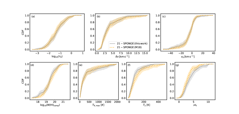
Figure 15: Comparison of cumulative distribution functions (CDFs) of parameters from the Gaussian fits to 21-SPONGE sources from this work (grey) and the analysis of Murray et al. (2018b, ; yellow (M18)), including amplitude ($\tau_{0}$; a), line width (FWHM; $\delta v$; b), mean velocity ($v_{0}$; c), and derived physical properties including column density (Equation 11, $N({\rm HI})_{\rm comp}$; e), maximum kinetic temperature (Equation 12, $T_{\rm K,max}$; e), spin temperature ($T_{s}$; f), and turbulent Mach number (Equation 13, $\mathcal{M}_{t}$; g). The uncertainty ranges in the CDFs are computed by bootstrapping the sample with replacement over $10^{4}$ trials, and illustrate the $1^{st}$ through $99^{\rm th}$ percentiles. We find that the method presented in this work (solid) is fully consistent with the results of the original 21-SPONGE analysis.

Appendix C Gaussian Fits to the Comparison Sample

In the following Appendix we present the results of autonomous, simultaneous decomposition of the comparison sample (21-SPONGE, Perseus, HT03). Figure 16 includes panels showing $T_{B}(v)$ (top panel) and $\tau_{\rm HI}(v)$ (bottom panel) for each of the $103$ LOS, including the best-fit components in absorption and their corresponding emission.

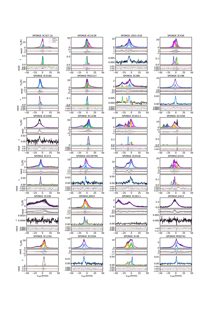
Figure 16: Gaussian fits to the comparison sample (SPONGE, HT03 and Perseus) $\tau_{\rm HI}(v)$ and $T_{B}(v)$ pairs using GaussPy. Each panel corresponds to a different sightline, including $T_{B}(v)$ from the $40$ off-positions (top panel), and $\tau_{\rm HI}(v)$ (bottom panel), with the total fits (dotted purple) to $\tau_{\rm HI}(v)$ (Equation 1; Murray et al., 2018b) and $T_{B}(v)$ (Equation 8), the individual components (solid, colors) and the residuals from the fits (sub-panels; grey), along with $\pm 3\sigma$ uncertainties (red).

References

- Astropy Collaboration et al. (2013) Astropy Collaboration, Robitaille, T. P., Tollerud, E. J., et al. 2013, A&A, 558, A33, doi: 10.1051/0004-6361/201322068
- Becker et al. (1995) Becker, R. H., White, R. L., & Helfand, D. J. 1995, ApJ, 450, 559, doi: 10.1086/176166
- Berkhuijsen et al. (1971) Berkhuijsen, E. M., Haslam, C. G. T., & Salter, C. J. 1971, A&A, 14, 252
- Clark (1965) Clark, B. G. 1965, ApJ, 142, 1398, doi: 10.1086/148426
- Clark et al. (2012) Clark, P. C., Glover, S. C. O., Klessen, R. S., & Bonnell, I. A. 2012, MNRAS, 424, 2599, doi: 10.1111/j.1365-2966.2012.21259.x
- Clark et al. (2015) Clark, S. E., Hill, J. C., Peek, J. E. G., Putman, M. E., & Babler, B. L. 2015, Phys. Rev. Lett., 115, 241302, doi: 10.1103/PhysRevLett.115.241302
- Clark et al. (2019) Clark, S. E., Peek, J. E. G., & Miville-Deschênes, M. A. 2019, ApJ, 874, 171, doi: 10.3847/1538-4357/ab0b3b
- Clark et al. (2014) Clark, S. E., Peek, J. E. G., & Putman, M. E. 2014, ApJ, 789, 82, doi: 10.1088/0004-637X/789/1/82
- Cox & Reynolds (1987) Cox, D. P., & Reynolds, R. J. 1987, ARA&A, 25, 303, doi: 10.1146/annurev.aa.25.090187.001511
- Dempsey et al. (2020) Dempsey, J., McClure-Griffiths, N. M., Jameson, K., & Buckland-Willis, F. 2020, MNRAS, 496, 913, doi: 10.1093/mnras/staa1602
- Dickey & Benson (1982) Dickey, J. M., & Benson, J. M. 1982, AJ, 87, 278, doi: 10.1086/113103
- Dickey & Lockman (1990) Dickey, J. M., & Lockman, F. J. 1990, ARA&A, 28, 215, doi: 10.1146/annurev.aa.28.090190.001243
- Dickey et al. (2000) Dickey, J. M., Mebold, U., Stanimirovic, S., & Staveley-Smith, L. 2000, ApJ, 536, 756, doi: 10.1086/308953
- Dickey et al. (1978) Dickey, J. M., Terzian, Y., & Salpeter, E. E. 1978, ApJS, 36, 77, doi: 10.1086/190492
- Dickey et al. (1981) Dickey, J. M., Weisberg, J. M., Rankin, J. M., & Boriakoff, V. 1981, A&A, 101, 332
- Dickey et al. (2013) Dickey, J. M., McClure-Griffiths, N., Gibson, S. J., et al. 2013, PASA, 30, e003, doi: 10.1017/pasa.2012.003
- Draine (2011) Draine, B. T. 2011, Physics of the Interstellar and Intergalactic Medium (Princeton University Press)
- Faucher-Giguère et al. (2015) Faucher-Giguère, C.-A., Hopkins, P. F., Kereš, D., et al. 2015, MNRAS, 449, 987, doi: 10.1093/mnras/stv336
- Gatto et al. (2015) Gatto, A., Walch, S., Low, M.-M. M., et al. 2015, MNRAS, 449, 1057, doi: 10.1093/mnras/stv324
- Gatto et al. (2017) Gatto, A., Walch, S., Naab, T., et al. 2017, MNRAS, 466, 1903, doi: 10.1093/mnras/stw3209
- Green et al. (2019) Green, G. M., Schlafly, E., Zucker, C., Speagle, J. S., & Finkbeiner, D. 2019, ApJ, 887, 93, doi: 10.3847/1538-4357/ab5362
- Greisen (2003) Greisen, E. W. 2003, Astrophysics and Space Science Library, Vol. 285, AIPS, the VLA, and the VLBA, ed. A. Heck, 109, doi: 10.1007/0-306-48080-8_7
- Grenier et al. (2005) Grenier, I. A., Casandjian, J.-M., & Terrier, R. 2005, Science, 307, 1292, doi: 10.1126/science.1106924
- Heiles (1976) Heiles, C. 1976, ApJ, 204, 379, doi: 10.1086/154181
- Heiles (1980) —. 1980, ApJ, 235, 833, doi: 10.1086/157685
- Heiles & Troland (2003a) Heiles, C., & Troland, T. H. 2003a, ApJS, 145, 329, doi: 10.1086/367785
- Heiles & Troland (2003b) —. 2003b, ApJ, 586, 1067, doi: 10.1086/367828
- HI4PI Collaboration et al. (2016a) HI4PI Collaboration, Ben Bekhti, N., Flöer, L., et al. 2016a, A&A, 594, A116, doi: 10.1051/0004-6361/201629178
- HI4PI Collaboration et al. (2016b) —. 2016b, A&A, 594, A116, doi: 10.1051/0004-6361/201629178
- Hopkins et al. (2014) Hopkins, P. F., Kereš, D., Oñorbe, J., et al. 2014, MNRAS, 445, 581, doi: 10.1093/mnras/stu1738
- Hunter (2007) Hunter, J. D. 2007, Computing In Science & Engineering, 9, 90, doi: 10.1109/MCSE.2007.55
- Kerp et al. (2011) Kerp, J., Winkel, B., Ben Bekhti, N., Flöer, L., & Kalberla, P. M. W. 2011, Astronomische Nachrichten, 332, 637, doi: 10.1002/asna.201011548
- Kim et al. (2014) Kim, C.-G., Ostriker, E. C., & Kim, W.-T. 2014, ApJ, 786, 64, doi: 10.1088/0004-637X/786/1/64
- Knapp (1975) Knapp, G. R. 1975, AJ, 80, 111, doi: 10.1086/111719
- Kuntz & Danly (1996) Kuntz, K. D., & Danly, L. 1996, ApJ, 457, 703, doi: 10.1086/176765
- Lallement et al. (2019) Lallement, R., Babusiaux, C., Vergely, J. L., et al. 2019, A&A, 625, A135, doi: 10.1051/0004-6361/201834695
- Lallement et al. (2003) Lallement, R., Welsh, B. Y., Vergely, J. L., Crifo, F., & Sfeir, D. 2003, A&A, 411, 447, doi: 10.1051/0004-6361:20031214
- Lee et al. (2015) Lee, M.-Y., Stanimirović, S., Murray, C. E., Heiles, C., & Miller, J. 2015, ApJ, 809, 56, doi: 10.1088/0004-637X/809/1/56
- Leike et al. (2020) Leike, R. H., Glatzle, M., & Enßlin, T. A. 2020, A&A, 639, A138, doi: 10.1051/0004-6361/202038169
- Lenz et al. (2017) Lenz, D., Hensley, B. S., & Doré, O. 2017, ApJ, 846, 38, doi: 10.3847/1538-4357/aa84af
- Lindner et al. (2015) Lindner, R. R., Vera-Ciro, C., Murray, C. E., et al. 2015, AJ, 149, 138, doi: 10.1088/0004-6256/149/4/138
- Liszt (1983) Liszt, H. S. 1983, ApJ, 275, 163, doi: 10.1086/161522
- McKee & Ostriker (1977) McKee, C. F., & Ostriker, J. P. 1977, ApJ, 218, 148, doi: 10.1086/155667
- Mebold (1972) Mebold, U. 1972, A&A, 19, 13
- Mebold et al. (1997) Mebold, U., Düsterberg, C., Dickey, J. M., Staveley-Smith, L., & Kalberla, P. 1997, ApJ, 490, L65, doi: 10.1086/311000
- Murray et al. (2020) Murray, C. E., Peek, J. E. G., & Kim, C.-G. 2020, ApJ, 899, 15, doi: 10.3847/1538-4357/aba19b
- Murray et al. (2018a) Murray, C. E., Peek, J. E. G., Lee, M.-Y., & Stanimirović, S. 2018a, ApJ, 862, 131, doi: 10.3847/1538-4357/aaccfe
- Murray et al. (2018b) Murray, C. E., Stanimirović, S., Goss, W. M., et al. 2018b, ApJS, 238, 14, doi: 10.3847/1538-4365/aad81a
- Murray et al. (2017) Murray, C. E., Stanimirović, S., Kim, C.-G., et al. 2017, ApJ, 837, 55, doi: 10.3847/1538-4357/aa5d12
- Murray et al. (2015) Murray, C. E., Stanimirović, S., Goss, W. M., et al. 2015, ApJ, 804, 89, doi: 10.1088/0004-637X/804/2/89
- Nguyen et al. (2019) Nguyen, H., Dawson, J. R., Lee, M.-Y., et al. 2019, ApJ, 880, 141, doi: 10.3847/1538-4357/ab2b9f
- Nguyen et al. (2018) Nguyen, H., Dawson, J. R., Miville-Deschênes, M. A., et al. 2018, ApJ, 862, 49, doi: 10.3847/1538-4357/aac82b
- Ntormousi et al. (2011) Ntormousi, E., Burkert, A., Fierlinger, K., & Heitsch, F. 2011, ApJ, 731, 13, doi: 10.1088/0004-637X/731/1/13
- Peek & Clark (2019) Peek, J. E. G., & Clark, S. E. 2019, ApJ, 886, L13, doi: 10.3847/2041-8213/ab53de
- Planck Collaboration et al. (2011) Planck Collaboration, Ade, P. A. R., Aghanim, N., et al. 2011, A&A, 536, A19, doi: 10.1051/0004-6361/201116479
- Radhakrishnan et al. (1972) Radhakrishnan, V., Murray, J. D., Lockhart, P., & Whittle, R. P. J. 1972, ApJS, 24, 15, doi: 10.1086/190248
- Reach et al. (2017a) Reach, W. T., Bernard, J.-P., Jarrett, T. H., & Heiles, C. 2017a, ApJ, 851, 119, doi: 10.3847/1538-4357/aa9b85
- Reach et al. (2017b) Reach, W. T., Heiles, C., & Bernard, J.-P. 2017b, ApJ, 834, 63, doi: 10.3847/1538-4357/834/1/63
- Remy et al. (2017) Remy, Q., Grenier, I. A., Marshall, D. J., & Casandjian, J. M. 2017, A&A, 601, A78, doi: 10.1051/0004-6361/201629632
- Rohlfs & Wilson (2004) Rohlfs, K., & Wilson, T. L. 2004, Tools of radio astronomy
- Roy et al. (2013) Roy, N., Kanekar, N., Braun, R., & Chengalur, J. N. 2013, MNRAS, 436, 2352, doi: 10.1093/mnras/stt1743
- Stanimirović et al. (2014) Stanimirović, S., Murray, C. E., Lee, M.-Y., Heiles, C., & Miller, J. 2014, ApJ, 793, 132, doi: 10.1088/0004-637X/793/2/132
- Van Der Walt et al. (2011) Van Der Walt, S., Colbert, S. C., & Varoquaux, G. 2011, Computing in Science & Engineering, 13, 22
- Vergely et al. (2010) Vergely, J. L., Valette, B., Lallement, R., & Raimond, S. 2010, A&A, 518, A31, doi: 10.1051/0004-6361/200913962
- Villagran & Gazol (2018) Villagran, M. A., & Gazol, A. 2018, MNRAS, 476, 4932, doi: 10.1093/mnras/sty438
- Winkel et al. (2010) Winkel, B., Kalberla, P. M. W., Kerp, J., & Flöer, L. 2010, ApJS, 188, 488, doi: 10.1088/0067-0049/188/2/488
- Winkel et al. (2016) Winkel, B., Kerp, J., Flöer, L., et al. 2016, A&A, 585, A41, doi: 10.1051/0004-6361/201527007
- Wolfire et al. (2003) Wolfire, M. G., McKee, C. F., Hollenbach, D., & Tielens, A. G. G. M. 2003, ApJ, 587, 278, doi: 10.1086/368016