Approximation Schemes for Capacitated Vehicle Routing on Graphs of Bounded Treewidth, Bounded Doubling, or Highway Dimension

Abstract

In this paper we present Approximation Schemes for Capacitated Vehicle Routing Problem (CVRP) on several classes of graphs. In CVRP, introduced by Dantzig and Ramser in 1959 [14], we are given a graph $G=(V,E)$ with metric edges costs, a depot $r\in V$, and a vehicle of bounded capacity $Q$. The goal is to find minimum cost collection of tours for the vehicle that return to the depot, each visiting at most $Q$ nodes, such that they cover all the nodes. This generalizes classic TSP and has been studied extensively. In the more general setting each node $v$ has a demand $d_{v}$ and the total demand of each tour must be no more than $Q$. Either the demand of each node must be served by one tour (unsplittable) or can be served by multiple tour (splittable). The best known approximation algorithm for general graphs has ratio $\alpha+2(1-\epsilon)$ (for the unsplittable) and $\alpha+1-\epsilon$ (for the splittable) for some fixed $\epsilon>\frac{1}{3000}$, where $\alpha$ is the best approximation for TSP. Even for the case of trees, the best approximation ratio is $4/3$ [5] and it has been an open question if there is an approximation scheme for this simple class of graphs. Das and Mathieu [15] presented an approximation scheme with time $n^{\log^{O(1/\epsilon)}n}$ for Euclidean plane $\mathbb{R}^{2}$. No other approximation scheme is known for any other class of metrics (without further restrictions on $Q$). In this paper we make significant progress on this classic problem by presenting Quasi-Polynomial Time Approximation Schemes (QPTAS) for graphs of bounded treewidth, graphs of bounded highway dimensions, and graphs of bounded doubling dimensions. For comparison, our result implies an approximation scheme for Euclidean plane with run time $n^{O(\log^{10}n/\epsilon^{9})}$.

1 Introduction

Vehicle routing problems (VRP) describe a class of problems where the objective is to find cost efficient delivery routes for delivering items from depots to clients using vehicles having limited capacity. These problems have numerous applications in real world settings. The Capacitated Vehicle Routing Problem (CVRP) was introduced by Dantzig and Ramser in 1959 [14]. In CVRP, we are given as input a graph $G=(V,E)$ with metric edge weights (also referred to as costs) $w(e)\in\mathbb{Z}^{\geq 0}$, a depot $r\in V$, along with a vehicle of capacity $Q>0$, and wish to compute a minimum weight/cost collection of tours, each starting from the depot and visiting at most $Q$ customers, whose union covers all the customers. In the more general setting each node $v$ has a demand $d(v)\in\mathbb{Z}^{\geq 1}$ and the goal is to find a set of tours of minimum total cost each of which includes $r$ such that the union of the tours covers the demand at every client and every tour covers at most $Q$ demand.

There are three common versions of CVRP: unit, splittable, and unsplittable. In the splittable variant, the demand of a node can be delivered using multiple tours, but in the unsplittable variant, the entire demand of a client must be delivered by a single tour. The unit demand case is a special case of the unsplittable case where every node has unit demand and the demand of a client must be delivered by a single tour. CVRP has also been referred to as the $k$-tours problem [3, 4]. All three variants admit constant factor approximation algorithm in polynomial-time [18]. Haimovich et al. [18] showed that a heuristic called iterative partitioning (which starts from a TSP tour and breaking the tour into capacity respecting tours by making a trip back and forth to the depot) implies an $(\alpha+1(1-1/Q))$-approximation for the unit demand case, with $\alpha$ being the approximation ratio of Traveling Salesman Problem (TSP). A similar approach implies a $2+(1-2/Q)\alpha)$-approximation for the unsplittable variant [2]. Very recently, Blauth et al. [10] improved these approximations by showing that there is an $\epsilon>0$ such that there is an $(\alpha+2\cdot(1-\epsilon))$-approximation algorithm for unsplittable CVRP and a $(\alpha+1-\epsilon)$-approximation algorithm for unit demand CVRP and splittable CVRP. For $\alpha=3/2$, they showed $\epsilon>1/3000$. All three variants are APX-hard in general metric spaces [25], so a natural research focus has been on structured metric spaces, i.e. special graph classes. Even on on trees (and in particular on stars) CVRP remains NP-hard [23], and there exists constant-factor approximations (currently being $4/3$ [5]), better than those for general metrics, however the following question has remained open:
Question. Is it possible to design an approximation scheme for CVRP on trees or more generally graphs of bounded treewidth?

We answer the above question affirmatively. For ease of exposition we start by prove the following first:

Theorem 1

For any $\epsilon>0$, there is an algorithm that, for any instance of the unit demand CVRP on trees outputs a $(1+\epsilon)$-approximate solution in time $n^{O(\log^{4}n/\epsilon^{3})}$. For any instance of the splittable CVRP on trees when $Q=n^{O(\log^{c}n)}$ the algorithm runs in time $n^{O(\log^{2c+4}n)}$.

We then show how this result can be extended to design QPTAS for graphs of bounded treewidth.

Theorem 2

For any $\epsilon>0$, there is an algorithm that, for any instance of the unit demand CVRP on a graph $G$ of bounded treewidth $k$ outputs a $(1+\epsilon)$-approximate solution in time $n^{O(k^{2}\log^{3}n/\epsilon^{2})}$. For the splittable CVRP on graphs of bounded treewidth when $Q=n^{O(\log^{c}n)}$, the algorithm outputs a $(1+\epsilon)$-approximate solution in time $n^{O(k^{2}\log^{2c+3}n/\epsilon^{2})}$.

As a consequence of this and using earlier results of embedding of graphs of bounded doubling dimensions or bounded highway dimensions into graphs of low treewidth we obtain approximation schemes for CVRP on those graph classes.

Theorem 3

For any $\epsilon>0$ and fixed $D>0$, there is a an algorithm that, given an instance of the splittable CVRP with capacity $Q=n^{\log^{c}n}$ on a graph of doubling dimension $D$, finds a $(1+\epsilon)$-approximate solution in time $n^{O(D^{D}\log^{2c+D+3}n/\epsilon^{D+2})}$.

As an immediate corollary, this implies an approximation scheme for CVRP on Euclidean metrics on $\mathbb{R}^{2}$ in time $n^{O(\log^{10}n/\epsilon^{9})}$ which improves on the run time of $n^{\log^{O(1/\epsilon)}n}$ of QPTAS of [15].

Theorem 4

For any $\epsilon>0,\lambda>0$ and $D>0$, there is a an algorithm that, given a graph with highway dimension $D$ with violation $\lambda$ as an instance of the splittable CVRP with capacity $Q=n^{\log^{c}n}$, finds a solution whose cost is at most $(1+\epsilon)$ times the optimum in time $n^{O(\log^{2c+3+\log^{2}(\frac{D}{\epsilon\lambda})\cdot\frac{1}{\lambda}}n/\epsilon^{2})}$.

1.1 Related Works

CVRP generalizes the classic TSP problem (with $Q=n$). For general metrics, Haimovich et al. [18] considered a simple heuristic, called tour partitioning, which starts from a TSP tour and then splits the tour into tours of size at most $Q$ (by making back-and-forth trips to $r$) and showed that it is a $(1+(1-1/Q)\alpha)$-approximation for splittable CVRP, where $\alpha$ is the approximation ratio for TSP. Essentially the same algorithm implies a $(2+(1-2/Q)\alpha)$-approximation for unsplittable CVRP [2]. These stood as the best known bounds until recently, when Blauth et al. [10] showed that given a TSP approximation $\alpha$, there is an $\epsilon>0$ such that there is an $(\alpha+2\cdot(1-\epsilon))$-approximation algorithm for CVRP. For $\alpha=3/2$, they showed $\epsilon>1/3000$. They also showed a $(\alpha+1-\epsilon)$-approximation algorithm for unit demand CVRP and splittable CVRP.

For the case of trees, Labbé et al. [23] showed splittable CVRP is NP-hard and Golden et al. [17] showed unsplittable version is APX-hard and hard to approximate better than 1.5. For splittable CVRP (again on trees), Hamaguchi et al. [19] defined a lower bound for the cost of the optimal solution and gave a 1.5 approximation with respect to the lower bound. Asano et al. [4] improved the approximation to $(\sqrt{41}-1)/4$ with respect to the same lower bound and also showed the existence of instances whose optimal cost is exactly 4/3 times the lower bound. Becker [5] gave a 4/3-approximation with respect to the lower bound. Becker and Paul [9] showed a $(1,1+\epsilon)$-bicriteria polynomial-time approximation scheme for splittable CVRP in trees, i.e. a PTAS but the capacity of every tour is up to $(1+\epsilon)Q$.

Das and Mathieu [15] gave a quasi-polynomial-time approximation scheme (QPTAS) for CVRP in the Euclidean plane ($\mathbb{R}^{2}$). A PTAS for when $Q$ is $O(\log n/\log\log n)$ or $Q$ is $\Omega(n)$ was shown by Asano et al. [4]. A PTAS for Euclidean plane $\mathbb{R}^{2}$ for all moderately large values of $Q\leq 2^{\log^{\delta}n}$, where $\delta=\delta(\epsilon)$, was shown by Adamaszek et al [1], building on the work of Das and Mathieu [15], and using it as a subroutine. For high dimensional Euclidean spaces $\mathbb{R}^{d}$, Khachay et al. [20] showed a PTAS when $Q$ is $O(\log^{1/d}n)$. For graphs of bounded doubling dimension, Khachay et al. [21] gave a QPTAS when the number of tours is $\mathop{\rm polylog}\nolimits(n)$ and Khachay et al. [22] gave a QPTAS when $Q$ is $\mathop{\rm polylog}\nolimits(n)$.

The following results are all for when $Q$ is a fixed. CVRP is APX-hard in general metrics and is polynomial-time solvable on trees. There exists a PTAS for CVRP in the Euclidean plane ($\mathbb{R}^{2}$) (again for when $Q$ is fixed) as shown by Khachay et al. [20]. A PTAS for planar graphs was shown by Becker et al. [8] and a QPTAS for planar and bounded-genus graphs was shown by Becker et al. [6]. A PTAS for graphs of bounded highway dimension and an exact algorithm for graphs with treewidth with running time $O(n^{\text{tw}Q})$ was shown by Becker et al [7]. Cohen-Addad et al. [12] showed an efficient PTAS for graphs of bounded-treewidth, an efficient PTAS for bounded highway dimension, an efficient PTAS for bounded genus metrics and a QPTAS for minor-free metrics. Again, note that these results are all under the assumption that $Q$ is fixed.

So aside from the QPTAS of [15] for $\mathbb{R}^{2}$ and subsequent slight generalization of [1] no approximation scheme is known for CVRP on any non-trivial metrics for arbitrary values of $Q$ (even for trees). Standard ways of extending a dynamic programs for Euclidean metrics to bounded doubling metrics do not seem to work to extend the results of [15] to doubling metrics in quasi-polynomial time.

1.2 Overview of our technique

We start by presenting a QPTAS for CVRP on trees and then extend the technique to graphs of bounded treewidth. Our main technique to design approximation scheme for CVRP is to show the existence of a near optimum solution where the sizes of the partial tours going past any node of the tree can be partitioned into only poly-logarithmic many classes. This will allow one to use dynamic programming to find a low cost solution. A simple rounding of tour sizes to some threshold values (e.g. powers of $(1+\epsilon)$) only works (with some care) to achieve a bi-criteria approximation as any under estimation of tour sizes may result in tours that are violating the capacities. To achieve a true approximation (without capacity violation) we show how we can break the tours of an optimum solution into "top" and "bottom" parts (at any node $v$) and then swap the bottom parts of tours with the bottom parts of other tours which are smaller, and then "round them up" to the nearest value from a set of poly-logarithmic threshold values. This swapping creates enough room to do the "round up" without violating the capacities. However, this will cause a small fraction of the vertices to become "not covered", we call them orphant nodes. We will show how we can randomly choose some tours of the optimum and add them back to the solution (at a small extra cost) and use these extra tours (after some modifications) to cover the orphant nodes. There are many details along the way. For instance, we treat the demand of each node as a token to be picked up by a tour. To ensure partial tour sizes are always from a small (i.e. poly-logarithmic) size set, we add extra tokens over the nodes. Also, for our QPTAS to work we need to bound the height of the tree. We show how we can reduce the height of the tree to poly-logarithmic at a small loss using a height reduction lemma that might prove useful for other vehicle routing problems.

The technique of QPTAS for trees then can be extended to graphs of bounded treewidth and also graphs of bounded doubling dimension; prove the existence of a similar near optimum solution and find one using dynamic program. Or one can use the known results for embedding of graphs of bounded doubling dimension into graphs of small treewidth.

2 Preliminaries

Recall that an instance ${\cal I}$ to CVRP is a graph $G=(V,E)$, where $w(e)$ is the cost or weight of edge $e\in E$ and $Q$ is the capacity of the vehicle. Each tour ${\cal T}$ is a walk over some nodes of $G$. We say $\cal T$ "covers" node $v$ if it serves the demand at node $v$. For the unit demand CVRP, it is easier to think of the demand of each node $v$ as being a token on $v$ that must be picked up by a tour. We can generalize this and assume each node $v$ can have multiple tokens and the total number of tokens a tour can pick is most $Q$ (possibly from the same or different locations). Note that each tour might visit vertices without picking any token there. The goal is to find a collection of tours of minimum total cost such that each token is picked up (or say covered) by some tour. We use $\mbox{\sc OPT}(G)$ or simply OPT to refer to an optimum solution of $G$, and opt to denote the value of it. Fix an optimal solution OPT. For any edge $e$ let $f(e)$ denote the number of tours travelling edge $e$ in OPT; so $\mbox{\sc opt}=\sum_{e}w(e)\cdot f(e)$.

First we show the demand of each node is bounded by a function of $Q$. And then, using standard scaling and rounding and at a small loss, we show we can assume the edge weights are polynomially bounded (in $n$). Given an instance for splittable CVRP with $n$ nodes and capacity $Q$, it is possible that the demand $d(v)>Q$ for some node $v$. From the work of Adamaszek et al [1], we will show how we can assume that the demand at each node $v$ satisfies $1\leq d(v)<nQ$. Adamaszek et al [1] defined a trivial tour to be a tour which picks up tokens from a single node in $T$ and a tour is non-trivial if the tour picks up tokens from at least two nodes in $T$. They defined a cycle to be a set of tours $t_{1},\ldots,t_{m}(m\geq 2)$ and a set of nodes $\ell_{1},\ell_{2},\ldots,\ell_{m},\ell_{m+1}=\ell_{1}$ such that each tour $t_{i}$ covers locations $\ell_{i}$ and $\ell_{i+1}$ and the origin is not considered as a node in $\ell_{1},\ldots,\ell_{m}$. They showed in Lemma 1 of [1] that there is an optimal solution in which there are no cycles. Since there are no 2-cycles, there are no two tours which cover the same pair of nodes. So there is an optimal solution such that there are at most $n$ non-trivial tours (as argued in [1]). So putting aside trivial tours (each picking up $Q$ tokens at a node), we can assume we have a total of at most $nQ$ tokens and in particular each node has at most this many tokens. Without loss of generality, we assume we have removed all trivial tours and so there is a total of at most $nQ$ demands.

We can also assume there is at most one tour in OPT covering at most $Q/2$ demand. If there are at least two tours ${\cal T}_{1}$ and ${\cal T}_{2}$ covering less than $Q/2$ demand, they can be merged into a single tour at no additional cost. Since the total demand is at most $nQ$, the total number of tours in the optimal solution is at most $nQ/(Q/2)=2n$.

Now we scale edge weights to be polynomially bounded. Observe that each tour in OPT traverses each edge $e$ at most once in each direction, so at most twice. Suppose we have guessed the largest edge weight that belongs to OPT (by enumerating over all possible such guesses) and have removed any edge with weight larger. Let $W=\max_{e\in E}w(e)$ be the largest (guessed) edge in OPT. Suppose we build instance ${\cal I}^{\prime}$ by rounding up the weight of each edge $e$ to be maximum of $w(e)$ and $\epsilon W/4n^{3}$. Since there are a total of at most $2n$ tours in OPT and each edge is traversed at most twice by each tour, and there are at most $n^{2}$ edges, the cost of solution OPT in ${\cal I}^{\prime}$ is at most $\mbox{\sc opt}+4n\cdot n^{2}\cdot\frac{\epsilon W}{4n^{3}}\leq(1+\epsilon)\mbox{\sc opt}$. Note that the ratio of maximum to minimum edge weight in ${\cal I}^{\prime}$ is $4n^{3}/\epsilon$, but the edge weights are not necessarily integer. Now suppose we scale the edge weights so that the minimum edge weight is 1 and the maximum edge weight is $4n^{3}/\epsilon$ and then scale them all by $1/\epsilon$, and then round each one up to the nearest integer. Note that by this rounding to the nearest integer, the cost of each edge is increased by a factor of at most $1+\epsilon$, so the cost of an optimum solution in the new instance is at most $(1+\epsilon)(1+\epsilon)=(1+O(\epsilon))$ factor larger than before rounding while the edge weights are all polynomially bounded integers. So from now on we assume we have this property for the given instance at a small loss.

We will use the following two simplified version of the Chernoff Bound [24] in our analysis.

Lemma 1 (Chernoff bound)

Let $Y=\sum_{i=1}^{n}Y_{i}$ where $Y_{i}=1$ with probability $p_{i}$ and 0 with probability $1-p_{i}$, and all $Y_{i}$’s are independent. With $\mu=\mathbb{E}{\left[Y\right]}$, $\mathbb{P}{\left[Y>2\mu\right]}\leq e^{-\mu/3}$ and $\mathbb{P}{\left[Y<\frac{\mu}{2}\right]}\leq e^{-\mu/8}.$

3 QPTAS for CVRP on Trees

In this section we prove Theorem 1. We will first prove a structure theorem which describes structural properties of a near-optimal solution. We will leverage these structural properties and use dynamic programming to compute a near-optimal solution.

3.1 Structure Theorem

Our goal in this section is to show the existence of a near optimum solution (i.e. one with cost $(1+O(\epsilon))\mbox{\sc opt}$) with certain properties which makes it easy to find one using dynamic programming. More specifically we show we can modify the instance ${\cal I}$ to instance ${\cal I}^{\prime}$ on the same tree $T$ where each node has $\geq 1$ tokens (so possibly more than 1) and change OPT to a solution $\mbox{\sc OPT}^{\prime}$ on ${\cal I}^{\prime}$ where cost of $\mbox{\sc OPT}^{\prime}$ is at most $(1+O(\epsilon))\mbox{\sc opt}$. Clearly the tours of $\mbox{\sc OPT}^{\prime}$ form a capacity respecting solution of ${\cal I}$ as well (of no more cost).

A starting point in our structure theorem is to show that given input tree $T$, for any $\epsilon>0$, we can build another tree $T^{\prime}$ of height $O(\log^{2}n/\epsilon)$ such that the cost of an optimum solution in $T^{\prime}$ is within $1+\epsilon$ factor of the optimum solution to $T$. We can lift a near-optimum solution to $T^{\prime}$ into a near-optimum solution of $T$. We will show the following in Subsection 3.6

Theorem 5

Given a tree $T$ as an instance of CVRP and for any fixed $\epsilon>0$, one can build a tree $T^{\prime}$ with height $\delta\log^{2}n/\epsilon$, for some fixed $\delta>0$, such that $\mbox{\sc opt}(T^{\prime})\leq\mbox{\sc opt}(T)\leq(1+\epsilon)\mbox{\sc opt}(T^{\prime})$.

So for the rest of this section we assume our input tree has height $O(\log^{2}n/\epsilon)$ at a loss of (yet another) $1+\epsilon$ in approximation ratio.

3.1.1 Overview of the ideas

Let us give a high level idea of the Structure theorem. In order to do that it is helpful to start from a simpler task of developing a bi-criteria approximation scheme

Let ${\cal T}$ be a tour in OPT and $v$ be a node in $T$. The coverage of ${\cal T}$ with respect to $v$ is the number of tokens picked by ${\cal T}$ in the subtree $T_{v}$.

Suppose a tour ${\cal T}$ visits node $v$. We refer to the subtour of ${\cal T}$ in $T_{v}$ (subtree rooted at $v$) as a partial tour.

A Bicriteria QPTAS: For simplicity, assume $T$ is binary (this is not crucial in the design of the DP). A subproblem would be based on a node $v\in T$ and the structure of partial tours going into $T_{v}$ to pick up tokens in $T_{v}$ at minimum cost. In other words, if one looks at the sections of tours of an optimum solution that cover tokens of $T_{v}$, what are the capacity profiles of those sections? For a vector $\vec{t}$ with $Q$ entries, where $\vec{t}_{i}$ (for each $1\leq i\leq Q)$ is the number of partial tours going down $T_{v}$ which pick $i$ tokens (or their capacity for that portion is $i$), entry $\textbf{A}[v,\vec{t}]$ would store the minimum cost of covering $T_{v}$ with (partial) tours whose capacity profile is given by $\vec{t}$. It is not hard to fill this table’s entries using a simple recursion based on the entries of children of $v$. So one can solve the CVRP problem "exactly" in time $O(n^{Q+1})$. We can reduce the time complexity by storing "approximate" sizes of the partial tours for each $T_{v}$. So let us "round" the capacities of the tours into $O(\log Q/\epsilon)$ buckets, where bucket $i$ represents capacities that are in $[(1+\epsilon)^{i-1},(1+\epsilon)^{i})$. More precisely, consider threshold-sizes $S=\{\sigma_{1},\ldots,\sigma_{\tau}\}$ where: for $1\leq i\leq 1/\epsilon$, $\sigma_{i}=i$, and for each value $i>1/\epsilon$: $\sigma_{i}=\sigma_{i-1}(1+\epsilon)$ and $\sigma_{\tau}=Q$. Note that $|S|=O(\log Q/\epsilon)=O(\log n/\epsilon)$. Suppose we allow each tour to pick up to $(1+\epsilon)Q$ tokens. If it was the case that each partial tour for $T_{v}$ (i.e. part of a tour that enters/exits $T_{v}$) has a capacity that is also threshold-size (this may not be true!) then the DP table entries would be based on vectors $\vec{t}$ of size $O(\log n/\epsilon)$, and the run time would be quasi-polynomial. One has to note that for each subproblem of the optimum at a node $v$ with children $u,w$, even if the tour sizes going down $T_{v}$ were of threshold-sizes, the partial tours at $T_{u}$ and $T_{w}$ do not necessarily satisfy this property.

To extend this to a proper bicriteria $(1+\epsilon)$-approximation we can define the thresholds based on powers of $1+\epsilon^{\prime}$ where $\epsilon^{\prime}=\frac{\epsilon^{2}}{\log^{2}n}$ instead: let $S=\{\sigma_{1},\ldots,\sigma_{\tau}\}$ where $\sigma_{i}=i$ for $1\leq i\leq 1/\epsilon^{\prime}$, and for $i>1/\epsilon^{\prime}$ we have $\sigma_{i}=\sigma_{i-1}(1+\epsilon^{\prime})$, and $\sigma_{\tau}=Q$. So now $|S|=O(\log^{2}n\cdot\log Q/\epsilon)=O(\log^{3}n/\epsilon^{2})$ when $Q=\text{poly}(n)$. For each vector $\vec{t}$ of size $\tau$, where $0\leq t_{i}\leq n$ is the number of partial tours with coverage/capacity $\sigma_{i}$, let $A[v,\vec{t}]$ store the minimum cost of a collection of (partial) tours covering all the tokens in $T_{v}$ whose capacity profile is $\vec{t}$, i.e. the number of tours of size in $[\sigma_{i},\sigma_{i+1})$ is $\vec{t}_{i}$. To compute the solution for $A[v,\vec{t}]$, given all the solutions for its two children $u,w$ we can do the following: consider two partial solutions, $A[u,\vec{t}_{u}]$ and $A[w,\vec{t}_{w}]$. One can combine some partial tours of $A[u,\vec{t}_{u}]$ with some partial tours of $A[w,\vec{t}_{w}]$, i.e. if ${\cal T}_{u}$ is a (partial) tour of class $i$ for $T_{u}$ and ${\cal T}_{w}$ is a partial tour of class $j$ for $T_{w}$ then either these two tours are in fact part of the same tour for $T_{v}$, or not. In the former case, the partial tour for $T_{v}$ obtained by the combination of the two tours will have cost $w({\cal T}_{u})+w({\cal T}_{w})+2w(vu)+2w(vw)$ and capacity $t_{i}+t_{j}$ (or possibly $t_{i}+t_{j}+1$ if this tour is to cover $v$ as well). In the latter case, each of ${\cal T}_{u}$ and ${\cal T}_{w}$ extend (by adding edges $vu$ and $vw$, respectively) into partial tours for $T_{v}$ of weights $w({\cal T}_{u})+2w(vu)$ and $w({\cal T}_{w})+2w(vw)$ (respectively) and capacities $t_{i}$ and $t_{j}$ (or perhaps $t_{i}+1$ or $t_{j}+1$ if one of them is to cover $v$ as well). In the former case, since $t_{i}+t_{j}$ is not a threshold-size, we can round it (down) to the nearest threshold-size. We say partial solutions for $T_{v}$, $T_{u}$ and $T_{w}$ are consistent if one can obtain the partial solution for $T_{v}$ by combining the solutions for $T_{v}$ and $T_{w}$. Given $A[v,\vec{t}]$, we consider all possible subproblems $A[u,\vec{t}_{u}]$ and $A[w,\vec{t}_{w}]$ that are consistent and take the minimum cost among all possible ways to combine them to compute $A[v,\vec{t}]$. Note that whenever we combine two solutions, we might be rounding the partial tour sizes down to a threshold-size, so we "under-estimate" the actual tour size by a factor of $1+\epsilon^{\prime}$ in each subproblem calculation. Since the height of the tree is $h=O(\log^{2}n/\epsilon)$, the actual error in the tour sizes computed at the root is at most $(1+\epsilon^{\prime})^{h}=(1+O(\epsilon))$, so each tour will have size at most $(1+O(\epsilon))Q$. The time to compute each entry $A[v,\vec{t}]$ can be upper bounded by $n^{O(\log^{3}n/\epsilon^{2})}$ and since there are $n^{O(\log^{3}n/\epsilon^{2})}$ subproblems, the total running time of the algorithm will be $n^{O(\log^{3}n/\epsilon^{2})}$. We can handle the setting where the tree is not binary (i.e. each node $v$ has more than two children) by doing an inner DP, like a knapsack problem over children of $v$ (we skip the details here as we will explain the details for the actual QPTAS instead).

Going from a Bicriteria to a true QPTAS: Our main tool to obtain a true approximation scheme for CVRP in trees is to show the existence of a near-optimum solution where the partial solutions for each $T_{v}$ have sizes that can be grouped into polyogarithmic many buckets as in the case of bi-criteria solution. Roughly speaking, starting from an optimum solution OPT, we follow a bottom-up scheme and modify OPT by changing the solution at each $T_{v}$: at each node $v$, we change the structure of the tours going down $T_{v}$ (by adding a few extra tours from the depot) and also adding some extra tokens at $v$ so that the partial tours that visit $T_{v}$ all have a size from one of polyogarithmic many possible sizes (buckets) while increasing the number and the cost of the tours by a small factor. We do this by duplicating some of the tours that visit $T_{v}$ while changing parts of them that go down in $T_{v}$ and adding some extra tokens at $v$: each tour still picks up at most a total of $Q$ tokens and the size (i.e. the number of tokens picked) for each partial tour in the subtree $T_{v}$ is one of $O(\log^{4}n/\epsilon^{2})$ many possible values, while the total cost of the solution is at most $(1+O(\epsilon))\mbox{\sc opt}$.

Suppose $T$ has height $h$ (where $h=\delta\log^{2}n/\epsilon$). Let $V_{\ell}$ (for $1\leq\ell\leq h$) be the set of vertices at level $\ell$ of the tree where $V_{1}=\{r\}$ and for each $\ell\geq 2$, $V_{\ell}$ are those vertices whose parent is in level $\ell-1$. For every tour ${\cal T}$ and every level $\ell$, the top part of ${\cal T}$ w.r.t. $\ell$ (denoted by ${\cal T}_{\ell}^{top}$), is the part of ${\cal T}$ induced by the vertices in $V_{1}\cup\ldots\cup V_{\ell-1}$ and the bottom part of ${\cal T}$ are the partial tours of ${\cal T}$ in the subtrees rooted at a vertex in $V_{\ell}$. Note that if we replace each partial tour of the bottom part of a tour ${\cal T}$ with a partial tour of a smaller capacity, the tour remains a capacity respecting tour. Consider a node $v$ (which is at some level $\ell$) and suppose we have $n_{v}$ partial tours covering $T_{v}$. Let the $n_{v}$ tours in increasing order of their coverage be $t_{1},\ldots,t_{n_{v}}$. Let $|t_{i}|$ be the coverage of tour $t_{i}$ (so $|t_{i}|\leq|t_{i+1}|$). For a $g$ (to be specified later), we add enough empty tours to the beginning of this list so that the number of tours is a multiple of $g$. Then, we will put these tours into groups $G^{v}_{1},\ldots,G^{v}_{g}$ of equal sizes by placing the $i$’th $n_{v}/g$ partial tours into $G^{v}_{i}$. Let $h^{v,max}_{i}$ ($h^{v,min}_{i}$) refer to the maximum (minimum) size of the tours in $G^{v}_{i}$. This grouping is similar to the grouping in the asymptotic PTAS for the classic bin-packing problem. Note that $h^{v,max}_{i}\leq h^{v,min}_{i+1}$.

Consider a mapping $f$ where it maps each partial tour in $G^{v}_{i}$ to one in $G^{v}_{i-1}$ in the same order, i.e. the largest partial tour in $G^{v}_{i}$ is mapped to the largest in $G^{v}_{i-1}$, the 2nd largest to the 2nd largest and so on, for $i>1$ (suppose $f(.)$ maps all the tours of $G^{v}_{1}$ to empty tours). Now suppose we modify OPT to $\mbox{\sc OPT}^{\prime}$ in the following way: for each tour ${\cal T}$ that has a partial tour $t\in G^{v}_{i}$, replace the bottom part of ${\cal T}$ at $v$ from $t$ to $f(t)$ (which is in $G^{v}_{i-1}$). Note that by this change, the size of any tour like ${\cal T}$ can only decrease. Also, if instead of $f(t)$ we had replaced $t$ with a partial tour of size $h^{v,max}_{i-1}$, it would still form a capacity respecting solution with the rest of ${\cal T}$, because $h^{v,max}_{i-1}\leq h^{v,min}_{i}\leq|t|$. The only problem is that those tokens in $T_{v}$ that were picked by the partial tours in $G^{v}_{g}$ are not covered by any tours; we call these orphant tokens. For now, assume that we add a few extra tours to OPT at low cost such that they cover all the orphant tokens of $T_{v}$. If we have done this change for all vertices $v\in V_{\ell}$, then for every tour like ${\cal T}$, the partial tours of ${\cal T}$ going down each $T_{v}$ (for $v\in V_{\ell}$) are replaced with partial tours from a group one index smaller. This means that, after these changes, for each tour ${\cal T}$ and its (new) partial tour $t\in G^{v}_{i}$, if we add $h^{v,max}_{i}-|t|$ extra tokens at $v$ to be picked up by $t$ then each partial tour has size exactly the same as the maximum size of its group without violating the capacities. This helps us store a compact "sketch" for partial solutions at each node $v$ with the property that the partial solution can be extended to a near optimum one.

How to handle the case of orphant tokens (those picked by the tours in the the last groups $G^{v}_{g}$ before the swap)? We will show that if $n_{v}$ is sufficiently large (at least polylogarithmic) then if we sample a small fraction of the tours of the optimum at random and add two copies of them (as extra tours), they can be used to cover the orphant tokens. So overall, we show how one can modify OPT by adding some extra tours to it at a cost of at most $\epsilon\cdot\mbox{\sc opt}$ such that: each node $v$ has $\geq 1$ tokens and the sketch of the partial tours at each node $v$ is compact (only polyogarithmic many possible sizes) while the dropped tokens overall can be covered by the extra tours.

3.1.2 Changing OPT to a near optimum structured solution

We will show how to modify the optimal solution OPT to a near-optimum solution $\mbox{\sc OPT}^{\prime}$ for a new instance ${\cal I}^{\prime}$ which has $\geq 1$ token at each node with certain properties. We start from $\ell=h$ and let $\mbox{\sc OPT}^{\prime}=\mbox{\sc OPT}_{\ell}=\mbox{\sc OPT}$ and for decreasing values of $\ell$, we will show how to modify $\mbox{\sc OPT}_{\ell+1}$ to obtain $\mbox{\sc OPT}_{\ell}$. To obtain $\mbox{\sc OPT}_{\ell}$ from $\mbox{\sc OPT}_{\ell+1}$ we keep the partial tours at levels $\geq\ell$ the same as $\mbox{\sc OPT}_{\ell+1}$ but we change the top parts of the tours and how the top parts can be matched to the partial tours at level $\ell$ so that together they form capacity respecting solutions (tours of capacity at most $Q$) at low cost.

First, we assume that OPT has at least $d\log n$ many tours for some sufficiently large $d$. Otherwise, if there are at most $D=d\log n$ many tours in OPT we can do a simple DP to compute OPT: for each node $v$, we have a sub problem $A[v,T^{v}_{1},\ldots,T^{v}_{D}]$ which stores the minimum cost solution if $T^{v}_{i}$ is the number of vertices the $i$’th tour is covering in the subtree $T_{v}$. It is easy to fill this table in time $O(n^{D})$ having computed the solutions for its children.

Definition 1

Let threshold values be $\{\sigma_{1},\ldots,\sigma_{\tau}\}$ where $\sigma_{i}=i$ for $1\leq i\leq\lceil 1/\epsilon\rceil$, and for $i>\lceil 1/\epsilon\rceil$ we have $\sigma_{i}=\lceil\sigma_{i-1}(1+\epsilon)\rceil$, and $\sigma_{\tau}=Q$. So $\tau=O(\log Q/\epsilon)$.

We consider the vertices of $T$ level by level, starting from nodes in level $V_{\ell=h-1}$ and going up, modifying the solution $\mbox{\sc OPT}_{\ell+1}$ to obtain $\mbox{\sc OPT}_{\ell}$.

Definition 2

For a node $v$, the $i$-th bucket, $b_{i}$, contains the number of tours of $\mbox{\sc OPT}_{\ell}$ having coverage between $[\sigma_{i},\sigma_{i+1})$ tokens in $T_{v}$ where $\sigma_{i}$ is the $i$-th threshold value. We will denote a node and bucket by a pair $(v,b_{i})$. Let $n_{v,i}$ be the number of tours in bucket $b_{i}$ of $v$.

Definition 3

A bucket $b$ is small if the number of tours in $b$ is at most $\alpha\log^{3}n/\epsilon^{2}$ and is big otherwise, for a constant $\alpha\geq\max\{1,12\delta\}$.

Note that for every node $v$ and bucket $b_{i}$ and for any two partial tours in $b_{i}$, the ratio of their size (coverage) is at most $(1+\epsilon)$. We will use this fact crucially later on. While giving the high level idea earlier in this section, we mentioned that we can cover the orphant tokens at low cost by using a few extra tours at low cost. For this to work, we need to assume that the ratio of the maximum size tour to the minimum size tour in all groups $G^{v}_{1},\ldots,G^{v}_{g}$ is at most $(1+\epsilon)$. To have this property, we need to do the grouping described for each vertex-bucket pair $(v,b_{i})$ that is big.

For each $v\in V_{\ell}$, let $(v,b_{i})$ be a vertex-bucket pair. If $b_{i}$ is a small bucket, we do not modify the partial tours in it. If $b_{i}$ is a big bucket, we create groups $G^{v}_{i,1},\ldots,G^{v}_{i,g}$ of equal sizes (by adding null/empty tours if needed to $G^{v}_{i,1}$ to have equal size groups), for $g=(2\delta\log n)/\epsilon^{2}$; so |$G^{v}_{i,j}|=\lceil n_{v,i}/g\rceil$. We also consider a mapping $f$ (as before) which maps (in the same order) the tours $t\in G^{v}_{i,j}$ to the tours in $G^{v}_{i,j-1}$ for all $1<j\leq g$. We assume the mapping maps tours of $G^{v}_{i,1}$ to empty tours. Let the size of the smallest (largest) partial tour in $G^{v}_{i,j}$ be $h^{v,min}_{i,j}$ ($h^{v,max}_{i,j}$). Note that $h^{v,max}_{i,j-1}\leq h^{v,min}_{i,j}$. Consider the set ${\bf T}_{\ell}$ of all the tours ${\cal T}$ in $\mbox{\sc OPT}_{\ell}$ that visit a vertex in one of the lower levels $V_{\geq\ell}$. Consider an arbitrary such tour ${\cal T}$ that has a partial tour $t$ in a big vertex/bucket pair $(v,b_{i})$, suppose $t$ belongs to group $G^{v}_{i,j}$. We replace $t$ with $f(t)$ in ${\cal T}$. Note that for ${\cal T}$, the partial tour at $T_{v}$ now has a size between $h^{v,min}_{i,j-1}$ and $h^{v,max}_{i,j-1}$. Now, add some extra tokens at $v$ to be picked up by ${\cal T}$ so that the size of the partial tour of ${\cal T}$ at $T_{v}$ is exactly $h^{v,max}_{i,j-1}$; note that since $h^{v,max}_{i,j-1}\leq|t|$, the new partial tour at $v$ can pick up the extra tokens without violating the capacity of ${\cal T}$. If we make this change for all tours ${\cal T}\in{\bf T}_{\ell}$, each partial tour of them at level $\ell$ that was in a group $j<g$ of a big vertex/bucket pair $(v,i)$ is replaced with a smaller partial tour from group $j-1$ of the same big vertex/bucket pair; after adding extra tokens at $v$ (if needed) the size is the maximum size from group $j-1$. All other partial tours (from small vertex/bucket pairs) remain unchanged. Also, the total cost of the tours has not increased (in fact some now have partial tours that are empty). However, the tokens that were picked by partial tours from $G^{v}_{i,g}$ for a big vertex/bucket pair $(v,b_{i})$ are now orphant. We describe how to cover them with some new tours.

One important observation is that when we make these changes, for any partial tours at vertices at lower levels ($V_{>\ell}$) their size remains the same. It is only the tour sizes going down a vertex at level $\ell$ that we are adjusting (by adding extra tokens). All other lower level partial tours remain unchanged (only their top parts may get swapped). This property holds inductively as we go up the tree and ensure that the lower level partial tours have one of polylogarithmic many sizes. More precisely, as we go up levels to compute $\mbox{\sc OPT}_{\ell}$, for any vertex $v^{\prime}\in V_{\ell^{\prime}}$ (where $\ell^{\prime}>\ell$) and any partial tour ${\cal T}^{\prime}$ visiting $T_{v^{\prime}}$, either $|{\cal T}^{\prime}|$ belongs to a small vertex bucket pair $(v^{\prime},b_{i^{\prime}})$ (and so has one of $O(\log^{3}n/\epsilon)$ many possible values) or if it belongs to a big vertex bucket pair $(v^{\prime},b_{i^{\prime}})$ then its size is equal to $h^{v^{\prime},max}_{i^{\prime},j^{\prime}}$ for some group $j^{\prime}$ and hence one of $O((\log Q\log n)/\epsilon^{2})$ possible values.

To handle (cover) orphant nodes, we are going to (randomly) select a subset of tours of OPT as "extra tours" and add them to $\mbox{\sc OPT}^{\prime}$ and modify them such that they cover all the tokens that are now orphant (i.e. those that were covered by partial tours of $G^{v}_{i,g}$ for all big vertex/bucket pairs at level $\ell$).

Suppose we select each tour ${\cal T}$ of OPT with probability $\epsilon$. We make two copies of the extra tour and we designate both extra copies to one of the levels $V_{\ell}$ that it visits with equal probability. We call these the extra tours.

Lemma 2

The cost of extra tours selected is at most $4\epsilon\cdot\mbox{\sc opt}$ w.h.p.

Proof. Recall that $f(e)$ denotes the number of tours passing through $e$ in OPT. The contribution of edge $e$ to the optimal solution is $2\cdot w(e)\cdot f(e)$ and we can write $\mbox{\sc opt}=\sum_{e\in E}2\cdot w(e)\cdot f(e)$. Let $e$ be the parent edge of a node in $v\in V_{\ell}$. Suppose an extra tour is designated to level $\ell$, we will only use it to cover orphant tokens from big buckets from nodes in $V_{\ell}$. A node $v$ would use an extra tour to cover orphant tokens only if one of $v$’s buckets is a big bucket. From now on, we will assume the extra tours only pass through an edge $e$ if $f(e)\geq\alpha\log^{3}n/\epsilon^{2}$ (we can shortcut it otherwise).

For an edge $e$, let $f^{\prime}(e)$ denote the number of sampled tours passing through $e$ and since we use two copies of each sampled tour, $2f^{\prime}(e)$ is the number of extra tours passing through $e$ in $\mbox{\sc OPT}^{\prime}$. We can write $\mbox{\sc opt}^{\prime}=\sum_{e\in E}2\cdot w(e)\cdot(f(e)+2f^{\prime}(e))$ and the cost of extra tours is $\sum_{e\in E}2\cdot w(e)\cdot 2f^{\prime}(e)$. While modifying OPT to $\mbox{\sc OPT}^{\prime}$, each tour in the optimal solution is sampled with probability $\epsilon$. Let $e$ be an edge with $f(e)$ tours ${\cal T}_{e,1},\ldots,{\cal T}_{e,f(e)}$ passing through it. Let $Y_{e,i}$ be a random variable which is 1 if tour ${\cal T}_{e,i}$ is sampled and $0$ otherwise.

$$\mathbb{E}{\left[Y_{e,i}\right]}=\mathbb{P}{\left[{\cal T}_{e,i}\text{ is sampled}\right]}=\epsilon.$$

Let $f^{\prime}(e)=Y_{e}=\sum_{i=1}^{f(e)}Y_{e,i}$. By linearity of expectations, we have

$$\mathbb{E}{\left[f^{\prime}(e)\right]}=\mathbb{E}{\left[Y_{e}\right]}=\sum_{i=1}^{f(e)}\mathbb{E}{\left[Y_{e,i}\right]}=\sum_{i=1}^{f(e)}\epsilon=\epsilon\cdot f(e).$$

Our goal is to show $\mathbb{P}{\left[Y_{e}>2\mathbb{E}{\left[Y_{e}\right]}\right]}$ is very low. Using Chernoff bound with $\mu=\mathbb{E}{\left[Y_{e}\right]}=\epsilon\cdot f(e)\geq\alpha\log^{3}n/\epsilon\geq 6\log n$.

$$\begin{split}\mathbb{P}{\left[Y_{e}>2\mathbb{E}{\left[Y_{e}\right]}\right]}&\leq e^{-(2\log n)}=\frac{1}{n^{2}}\end{split}$$

The above concentration bound holds for a single edge $e$. Using the union bound, we can show this hold with high probability over all edges,

$$\sum_{e\in E}\mathbb{P}{\left[Y_{e}>2\mathbb{E}{\left[Y_{e}\right]}\right]}\leq\frac{1}{n}.$$

We showed $f^{\prime}(e)\leq 2\epsilon\cdot f(e)$ with high probability. Hence, with high probability, the cost of the extra tours is at most

$$\sum_{e\in E}2\cdot w(e)\cdot 2f^{\prime}(e)\leq\sum_{e\in E}2\cdot w(e)\cdot 4\epsilon\cdot f(e)=4\epsilon\sum_{e\in E}2\cdot w(e)\cdot f(e)=4\epsilon\cdot\mbox{\sc opt}.$$

 

Therefore, we can assume that the cost of all the extra tours added is at most $4\epsilon\cdot\mbox{\sc opt}$. Let $X_{\ell}$ be the set of extra tours designated to level $\ell$. We assume we add $X_{\ell}$ when we are building $\mbox{\sc OPT}_{\ell}$ (it is only for the sake of analysis). For each $v\in V_{\ell}$ and vertex/bucket pair $(v,b_{i})$, let $X_{v,i}$ be those in $X_{\ell}$ whose partial tour in $T_{v}$ has a size in bucket $b_{i}$. Each extra tour in $X_{\ell}$ will not be picking any of the tokens in levels $V_{<\ell}$ (as they will be covered by the tours already in $\mbox{\sc OPT}_{\ell}$); they are used to cover the orphant tokens created by partial tours of $G^{v}_{i,g}$ for each big vertex/bucket pair $(v,b_{i})$ with $v\in V_{\ell}$; as described below.

Lemma 3

For each level $V_{\ell}$, each vertex $v\in V_{\ell}$ and big vertex/bucket pair $(v,b_{i})$, w.h.p. $|X_{v,i}|\geq\frac{\epsilon^{2}}{\delta\log^{2}n}\cdot n_{v,i}$.

Proof. Suppose $(v,b_{i})$ is a big vertex/bucket pair at some level $V_{\ell}$. Let $p_{1},\ldots,p_{n_{v,i}}$ be the partial tours in vertex/bucket pair $(v,b_{i})$. Let the tour in OPT corresponding to $p_{i}$ be ${\cal T}$. Two copies of tour $p_{i}$ are assigned to $b_{i}$ if both of the following events are true:

• Let $A_{i}$ be the event where tour ${\cal T}$ is sampled as an extra tour. Since each tour is sampled with probability $\epsilon$, we have $\mathbb{P}{\left[A_{i}\right]}=\epsilon$.

• Let $B_{i}$ be the event where tour ${\cal T}$ is assigned to level $\ell$. There are $h=\delta\log^{2}n/\epsilon$ many levels and since ${\cal T}$ (if sampled) is assigned to any one of its levels, $\mathbb{P}{\left[B_{i}\right]}\geq 1/h\geq\epsilon/(\delta\log^{2}n)$.

Let $Y_{i}$ be a random variable which is 1 if $p_{i}$ is an extra tour in $(v,b_{i})$ and 0 otherwise.

$$\mathbb{E}{\left[Y_{i}\right]}=\mathbb{P}{\left[Y_{i}=1\right]}=\mathbb{P}{\left[A_{i}\land B_{i}\right]}=\mathbb{P}{\left[A_{i}\right]}\cdot\mathbb{P}{\left[B_{i}\right]}\geq\epsilon^{2}/(\delta\log^{2}n).$$

Let $Y_{v,i}=\sum_{i=1}^{n_{v,i}}Y_{i}$ be the random variable keeping track of the number of sampled tours in $(v,b_{i})$. The number of extra tours, $|X_{v,i}|=2Y_{v,i}$ since we add two copies of a sampled tour to $X_{v,i}$. By linearity of expectation, we have

$$\mathbb{E}{\left[|X_{v,i}|\right]}=2\mathbb{E}{\left[Y_{v,i}\right]}=2\sum_{i=1}^{n_{v,i}}\mathbb{E}{\left[Y_{i}\right]}\geq\frac{2\epsilon^{2}}{\delta\log^{2}n}\cdot n_{v,i}.$$

We want to show that $|X_{v,i}|\geq\frac{\mathbb{E}{\left[|X_{v,i}|\right]}}{2}\geq\frac{\epsilon^{2}}{\delta\log^{2}n}\cdot n_{v,i}$ with high probability over all vertex-bucket pairs.

Using Chernoff Bound with $\mu=\mathbb{E}{\left[|X_{v,i}|\right]}\geq\frac{2\epsilon^{2}}{\delta\log^{2}n}\cdot n_{v,i}\geq 24\log n$ since $n_{v,i}\geq\alpha\log^{3}n/\epsilon^{2}$ and $\alpha\geq 12\delta$.

$$\begin{split}\mathbb{P}{\left[|X_{v,i}|<\frac{\mathbb{E}{\left[|X_{v,i}|\right]}}{2}\right]}&\leq e^{-(3\log n)}=\frac{1}{n^{3}}\end{split}$$

Note that the above equation only shows the concentration bound for a single vertex/bucket pair. There are $n$ nodes and each node has up to $\tau=\log n/\epsilon$ buckets, so the total number of vertex/bucket pairs is at most $n\log n/\epsilon$. Suppose we do a union bound over all buckets, we get

$$\sum_{\text{all }(v,b_{i})\text{ pairs}}\mathbb{P}{\left[|X_{v,i}|<\frac{\mathbb{E}{\left[|X_{v,i}|\right]}}{2}\right]}\leq\frac{1}{n}.$$

We showed that for each vertex/bucket pair $v,b_{i}$, $|X_{v,i}|\geq\frac{\epsilon^{2}}{\delta\log^{2}n}n_{v,i}\geq\alpha\log n/(2\delta)$ holds with high probability.  

Lemma 4

Consider all $v\in V_{\ell}$, big vertex/bucket pairs $(v,b_{i})$ and partial tours in $G^{v}_{i,g}$. We can modify the tours in $X_{v,i}$ (without increasing the cost) and adding some extra tokens at $v$ (if needed) so that:

1. The tokens picked up by partial tours in $G^{v}_{i,g}$ are covered by some tour in $X_{v,i}$, and

2. The new partial tours that pick up the orphant tokens in $G^{v}_{i,g}$ have size exactly $h^{v,max}_{i,g}$ and all tours still have size at most $Q$.

3. For each (new) partial tour of $X_{v,i}$ and every level $\ell^{\prime}>\ell$, the size of partial tours of $X_{v,i}$ at a vertex at level $\ell^{\prime}$ is also one of $O(\log Q\log^{3}n/\epsilon^{3})$ many sizes.

Proof. Our goal is to use the extra tours in $X_{v,i}$ to cover tokens picked up by partial tours of $G^{v}_{i,g}$ and we want each extra tour in $X_{v,i}$ to cover exactly $h^{v,max}_{i,g}$ tokens. The tours in the last group, $G^{v}_{i,g}$, cover $\sum_{t\in G^{v}_{i,g}}|t|$ many tokens. Since we want each tour in $X_{v,i}$ to cover $h^{v,max}_{i,g}$ tokens, we will add $\sum_{t\in G^{v}_{i,g}}(h^{v,max}_{i,g}-|t|)$ extra tokens at $v$ for each vertex/bucket pair $(v,b_{i})$ so that there are $h^{v,max}_{i,g}$ tokens for each partial tour in $G^{v}_{i,g}$. From now on, we will assume each partial tour in a last group $G^{v}_{i,g}$ covers $h^{v,max}_{i,g}$ tokens.

We know $|G^{v}_{i,g}|=n_{v,i}/g=\frac{\epsilon^{2}}{2\delta\log n}\cdot n_{v,i}$. Using Lemma 3, we know with high probability that $|X_{v,i}|\geq\frac{\epsilon^{2}}{\delta\log^{2}n}\cdot n_{v,i}=2|G^{v}_{i,g}|$, so $|X_{v,i}|/|G^{v}_{i,g}|\geq 2$. Recall $\mbox{\sc OPT}^{\prime}$ includes tours in OPT plus the extra tours in OPT that were sampled. Let $Y_{v,i}$ denote the number of tours in vertex/bucket pair $(v,b_{i})$ that were sampled, so $|X_{v,i}|=2|Y_{v,i}|$ since we made two extra copies of each sampled tour and $|Y_{v,i}|\geq|G^{v}_{i,g}|$ with high probability. We will start by creating a one-to-one mapping $s:G^{v}_{i,g}\rightarrow Y_{v,i}$ which maps each tour in $G^{v}_{i,g}$ to a sampled tour in $Y_{v,i}$. We know such a one-to-one mapping exists since $|Y_{v,i}|\geq|G^{v}_{i,g}|$.

Let ${\cal T}$ be a sampled tour in $Y_{v,i}$ with two extra copies of it, ${\cal T}_{1}$ and ${\cal T}_{2}$ in $X_{v,i}$. Let the partial tours of ${\cal T}$ at the bottom part in $V_{\ell}$ be $p_{1},\ldots,p_{m}$. We know $|{\cal T}|\geq\sum_{i=1}^{m}|p_{i}|$. Since $s$ is one-to-one, one partial tour from $r_{k}\in G^{v}_{i,g}$ maps to $p_{j}$ or no tour maps to $p_{j}$. If no tour maps to $p_{j}$, we consider the load assigned to $p_{j}$ to be zero. If $s(r_{k})=p_{j}$ where $r_{k}\in G^{v}_{i,g}$, since we added extra tokens to make each partial tour $r_{k}\in G^{v}_{i,g}$ have $h^{v,max}_{i,g}$ tokens, the load assigned to $p_{j}$ would be $h^{v,max}_{i,g}$.

Suppose we think of $r_{1},\ldots,r_{m}$ as items and ${\cal T}_{1}$ and ${\cal T}_{2}$ as bins of size $Q$. We know each $r_{i}$ fits into a bin of size $Q$. Recall that for the tour $r_{j}$ assigned to $p_{j}$, we know $|r_{j}|\leq(1+\epsilon)|p_{j}|$ since both $r_{j}$ and $p_{j}$ are in the same group $G^{v}_{i,g}$. We might not be able to fit all items $r_{1},\ldots,r_{m}$ into a bin of size $Q$ because $\sum_{i=1}^{m}|r_{i}|\leq(1+\epsilon)\sum_{i=1}^{m}|p_{i}|\leq(1+\epsilon)|{\cal T}|\leq(1+\epsilon)Q$. However, if we used two bins of size $Q$, we can pack the items into both bins without exceeding the capacity of either bin such that each item $r_{i}$ is completely in one bin. Since ${\cal T}_{1}$ and ${\cal T}_{2}$ are not assigned to any lower level, they have not been used to cover any tokens so far in our algorithm and they both have unused capacity $Q$. Using the bin packing analogy, we could split $r_{1},\ldots,r_{m}$ between ${\cal T}_{1}$ and ${\cal T}_{2}$. We could assign $r_{1},\ldots,r_{j}$ (for the maximum $j$) to ${\cal T}_{1}$ such that $\sum_{i=1}^{j}|r_{i}|\leq Q$ and the rest, $r_{j+1},\ldots,r_{m}$ to ${\cal T}_{2}$. Since $\sum_{i=1}^{m}|r_{i}|\leq(1+\epsilon)Q$, we can ensure we can distribute the tokens in $r_{i}$’s amongst ${\cal T}_{1}$ and ${\cal T}_{2}$ such that both ${\cal T}_{1}$ and ${\cal T}_{2}$ cover at most $Q$ tokens. Although there are two copies of each partial tour $p_{i}$ in $X_{v,i}$, according to our approach, we are using at most one of them (their coverage would be zero if they are not used). If the coverage of one of the extra partial tours is non-zero, we also showed that if it picks up tokens from a partial tour in $G^{v}_{i,g}$, it would pick up exactly $h^{v,\max}_{i,g}$ tokens, proving the 2nd property of the Lemma.

Also, note that for each partial tour $r_{k}\in G^{v}_{i,g}$ and for each level $\ell^{\prime}>\ell$ if $r_{k}$ visits a vertex $v^{\prime}\in V_{\ell^{\prime}}$, then the partial tour of $r_{k}$ at $T_{v^{\prime}}$ already satisfies the properties that: either its size belongs to a small vertex-bucket pair $(v^{\prime},b_{i})$ (so has one of $O(\log^{3}n/\epsilon)$ many possible values) or if it belongs to a big vertex bucket pair $(v^{\prime},b_{i^{\prime}})$ then its size is equal to $h^{v^{\prime},max}_{i^{\prime},j^{\prime}}$ for some group $j^{\prime}$ and hence one of $O((\log Q\log n)/\epsilon^{2})$ possible values. This implies that for the extra tours of $X_{v,i}$, after we reassign partial tours of $G^{v}_{i,g}$ to them (to cover the orphant nodes), each will have a size exactly equal to $h^{v,max}_{i,g}$ at level $\ell$ and at lower levels $V_{>\ell}$ they already have one of the $O(\log Q\log^{3}n/\epsilon^{3})$ many possible sizes. This establishes the 3rd property of the lemma.  

Therefore, using Lemma 4, all the tokens of $T_{v}$ remain covered by partial tours; those partial tours in $G^{v}_{i,j}$ (for $1\leq j<g$) are tied to the top parts of the tours from group $G^{v}_{i,j+1}$ and the partial tours of $G^{v}_{i,g}$ will be tied to extra tours designated to level $\ell$. We also add extra tokens at $v$ to be picked up by the partial tours of $T_{v}$ so that each partial tour has a size exactly equal to the maximum size of a group. All in all, the extra cost paid to build $\mbox{\sc OPT}_{\ell}$ (from $\mbox{\sc OPT}_{\ell+1}$) is for the extra tours designated to level $\ell$.

Theorem 6

(Structure Theorem) Let opt be the cost of the optimal solution to instance ${\cal I}$. We can build an instance ${\cal I}^{\prime}$ on the same tree $T$ such that each node has $\geq 1$ tokens and there exists a near-optimal solution $\mbox{\sc OPT}^{\prime}$ for ${\cal I}^{\prime}$ having cost $(1+4\epsilon)\mbox{\sc opt}$ w.h.p with the following property. The partial tours going down subtree $T_{v}$ for every node $v$ in $\mbox{\sc OPT}^{\prime}$ has one of $O((\log Q\log^{3}n)/\epsilon^{3})$ possible sizes. More specifically, suppose $(v,b_{i})$ is a bucket pair for $\mbox{\sc OPT}^{\prime}$. Then either:

• $b_{i}$ is a small bucket and hence there are at most $\alpha\log^{3}n/\epsilon^{2}$ many partial tours of $T_{v}$ whose size is in bucket $b_{i}$, or

• $b_{i}$ is a big bucket; in this case there are $g=(2\delta\log n)/\epsilon^{2}$ many group sizes in $b_{i}$: $\sigma_{i}\leq h^{v,max}_{i,1}\leq\ldots\leq h^{v,max}_{i,g}<\sigma_{i+1}$ and every tour of bucket $i$ has one of these sizes.

Proof. We will show how to modify OPT to a near-optimal solution $\mbox{\sc OPT}^{\prime}$. We start from $\ell=h$ and let $\mbox{\sc OPT}_{\ell}=\mbox{\sc OPT}$. For decreasing values of $\ell$ we show, for each $\ell$ how to modify $\mbox{\sc OPT}_{l+1}$ to obtain $\mbox{\sc OPT}_{\ell}$. We do this in the following manner: we do not modify partial tours in small buckets. However, for tours in big buckets, in each vertex/bucket pair $(v,b_{i})$ in level $\ell-1$, we place them into $g$ groups $G_{1}^{v},\ldots,G^{v}_{g}$ of equal sizes by placing the $i$’th $n_{v}/g$ partial tours into $G_{i}^{v}$. We have a mapping $f$ from each partial tour in $G^{v}_{i-1}$ to one in $G^{v}_{i}$ for $i\in\{2,\ldots,g\}$. We modify $\mbox{\sc OPT}_{\ell}$ to $\mbox{\sc OPT}_{\ell+1}$ in the following way: for each tour ${\cal T}$ that has a partial tour $t\in G_{i}^{v}$, replace the bottom part of ${\cal T}$ at $v$ from $t$ to $f(t)$ (which is in $G^{v}_{i-1}$). For each tour $t\in G^{v}_{i-1}$, we will add $h^{v,\max}_{i-1}-|t|$ many extra tokens at $v$. Note that by this change, the size of any tour such as ${\cal T}$ can only decrease and we are not violating feasibility of the tour because $h^{v,\max}_{i-1}\leq h_{i}^{v,\min}$. However, the tokens in $T_{v}$ picked up by the partial tours in $G^{v}_{i,g}$ are not covered by any tours. We can use Lemma 4 to show how we can use extra tours to cover the partial tours in $G^{v}_{i,g}$ such that the new partial tours have size exactly $h^{v,\max}_{i,g}$.

We will inductively repeat this for levels $\ell-2,\ell-3,\ldots,1$ and obtain $\mbox{\sc OPT}_{1}=\mbox{\sc OPT}^{\prime}$. Note that by adding extra tokens $h^{v,\max}_{i-1}-|t|$ for a tour $t\in G^{v}_{i-1}$, we are enforcing that the coverage of each tour is the maximum size of tours in its group. In a big bucket, there are $g=(2\delta\log n)/\epsilon^{2}$ many group sizes, so there are $O(\log n/\epsilon^{2})$ possible sizes for tours in big buckets at a node. In a small bucket, there can be at most $\alpha\log^{3}n/\epsilon^{2}$ many tours and since there are $\tau=O(\log Q/\epsilon)$ many buckets, there can be at most $O((\log Q\log^{3}n)/\epsilon^{3})$ many tour sizes covering $T_{v}$.

Using Lemma 2, we know the cost of the extra tours is at most $4\epsilon\cdot\mbox{\sc opt}$ with high probability, so the cost of $\mbox{\sc opt}^{\prime}\leq(1+4\epsilon)\mbox{\sc opt}$.  

3.2 Dynamic Program

In this section we complete the proof of Theorem 1. We will describe how we can compute a solution of cost at most $(1+4\epsilon)\mbox{\sc opt}$ using dynamic programming and based on the existence of a near-optimum solution guaranteed using the structure theorem. For each vertex/bucket pair, we do not know if the bucket is small or big, so we will consider subproblems corresponding to both possibilities. Informally, we will have a vector $\vec{n}\in[n]^{\tau}$ where if $i<1/\epsilon$, $n_{i}$ keeps track of the exact number of tours of size $i$ and for $i\geq 1/\epsilon$, $\vec{n}_{i}$ keeps track of the number of tours in bucket $b_{i}$, or tours covering between $[\sigma_{i},\sigma_{i+1})$ tokens. Let $o_{v}$ denote the total number of tokens to be picked up across all nodes in the subtree $T_{v}$. Since each node has at least one token, $o_{v}\geq|V(T_{v})|$. We will keep track of three other pieces of information conditioned on whether $b_{i}$ is a small or big bucket. If $b_{i}$ is a small bucket, we will store all the tour sizes exactly. Since the number of tours in a small bucket is at most $\gamma=\alpha\log^{3}n/\epsilon^{2}$, we will use a vector $\vec{t}^{i}\in[n]^{\gamma}$ to represent the tours of a small bucket where $\vec{t}^{i}_{j}$ represents the size of $j$-th tour in bucket $b_{i}$. Suppose $b_{i}$ is a big bucket, there are $g=(2\delta\log n)/\epsilon^{2}$ many tour sizes in the bucket corresponding to $n^{g}$ possibilities. For each big bucket $b_{i}$ at node $v$, we need to keep track of the following information,

• $\vec{h}^{i}_{v}\in[n]^{g}$ is a vector where $\vec{h}^{i}_{v,j}=h^{v,\max}_{i,j}$, which is the size of the maximum tour in group $j$ of bucket $i$ at node $v$.

• $\vec{l}^{i}_{v}\in[n]^{g}$ is a vector where $\vec{l}^{i}_{v,j}$ denotes the number of partial tours covering $h^{v,\max}_{i,j}$ tokens which lies in group $j$ of bucket $i$ at node $v$.

Let $\vec{y}_{v}$ denote a configuration of tours across all buckets of $v$.

$$\vec{y}_{v}=[o_{v},\vec{n}_{v},(\vec{t}_{v}^{1},\vec{h}_{v}^{1},\vec{l}_{v}^{1}),(\vec{t}_{v}^{2},\vec{h}_{v}^{2},\vec{l}_{v}^{2}),\ldots,(\vec{t}_{v}^{\tau},\vec{h}_{v}^{\tau},\vec{l}_{v}^{\tau})].$$

Note that a bucket $b_{i}$ is either small or big and cannot be both, hence given $(\vec{t}^{i}_{v},\vec{h}^{i}_{v},\vec{l}^{i}_{v})$, it cannot be the case that $\vec{t}^{i}_{v}\neq\vec{0},\vec{h}^{i}_{v}\neq\vec{0}$ and $\vec{l}^{i}_{v}\neq\vec{0}$. The subproblem $\textbf{A}[v,\vec{y}]$ is supposed to be the minimum cost collection of partial tours going down $T_{v}$ (to cover the tokens in $T_{v}$) and the cost of using the parent edge of $v$ having tour profile corresponding to $\vec{y}$. Our dynamic program heavily relies on the properties of the near-optimal solution in the structure theorem. Let $v$ be a node. We will compute $A[\cdot,\cdot]$ in a bottom-up manner, computing $\textbf{A}[v,\vec{y}_{v}]$ after we have computed the entries for the children of $v$.

The final answer is obtained by looking at the various entries of $\textbf{A}[r,\cdot]$ and taking the smallest one. First, we argue why this will correspond to a solution of cost no more than $\mbox{\sc opt}^{\prime}$. We will compute our solution in a bottom-up manner.

For the base case, we consider leaf nodes. A leaf node $v$ with parent edge $e$ could have $o_{v}\geq 1$ tokens at $v$. We will set $\textbf{A}[v,\vec{y}_{v}]=2\cdot w(e)\cdot m_{v}$ where $m_{v}$ is the number of tours in $\vec{y}_{v}$ if the total sum of tokens picked up by the partial tours in $\vec{y}_{v}$ is exactly $o_{v}$. Recall that $f(e)$ is the load on (i.e. number of tours using) edge $e$. From our structure theorem, we know there exists a near optimum solution such that each partial tour of $T_{v}$ has one of $O((\log Q\log^{3}n)/\epsilon^{3})$ tour sizes and for each small bucket, there are at most $\alpha\log^{3}n/\epsilon^{2}$ partial tours in it. For every big bucket, there are $g=(2\delta\log n)/\epsilon^{2}$ many group sizes and every tour of bucket $i$ has one of these sizes. The base case follows directly from the structure theorem.

To compute cell $\textbf{A}[v,\vec{y}_{v}]$, we would need to use another auxiliary table B. Suppose $v$ has $k$ children $u_{1},\ldots,u_{k}$ and assume we have already calculated $\textbf{A}[u_{j},\vec{y}]$ for every $1\leq j\leq k$ and for all vectors $\vec{y}$. Then we define a cell in our auxiliary table $\textbf{B}[v,\vec{y}_{v}^{\prime},j]$ for each $1\leq j\leq k$ where $\textbf{B}[v,\vec{y}_{v}^{\prime},j]$ is the minimum cost of covering $T_{u_{1}}\cup\ldots\cup T_{u_{j}}$ where $\vec{y}_{v}^{\prime}$ is the tour profile for the union of subtrees $T_{u_{1}}\cup\ldots\cup T_{u_{j}}$. In other words, $\textbf{B}[v,\vec{y}_{v}^{\prime},j]$ is what $\textbf{A}[v,\vec{y}_{v}]$ is supposed to capture when restricted only to the first $j$ children of $v$. We will set $\textbf{A}[v,\vec{y}_{v}]=\textbf{B}[v,\vec{y}_{v}^{\prime},k]+2\cdot w(e)\cdot m_{v}$ where $m_{v}$ is the number of different tours in $\vec{y}_{v}^{\prime}$. We will assume the parent edge of the depot has weight 0. Suppose $T_{u_{i}}$ has $o_{i}$ tokens, then the number of tokens in $T_{v}$ is at least $1+\sum_{i=1}^{k}o_{i}$. To compute entries of $\textbf{B}[v,\cdot,\cdot]$, we use both A and B entries for smaller subproblems of $v$ in the following way:

Case 1: j = 1: This is the case when we restrict the coverage to only the first child of $v$, $u_{1}$.

$$\begin{split}\textbf{B}[v,\vec{y}_{v}^{\prime},1]&=\underset{\vec{y}^{\prime}}{\text{min }}\left\{\textbf{A}[u_{1},\vec{y}^{\prime}]\right\}\\ \end{split}$$

We will find the minimum cost configurations $\vec{y}^{\prime}$ such that $\vec{y}_{v}^{\prime}$ and $\vec{y}^{\prime}$ are consistent with each other. We say $\vec{y}_{v}^{\prime}$ and $\vec{y}^{\prime}$ are consistent if a tour in $\vec{y}_{v}^{\prime}$ either only covers tokens at $v$ and does not visit any node below $v$ or $\vec{y}_{v}^{\prime}$ consists of a tour from $\vec{y}^{\prime}$ plus zero or more extra tokens picked up at $v$. Moreover, every tour in $\vec{y}^{\prime}$ is part of some tour in $\vec{y}_{v}^{\prime}$.

Case 2: $2\leq j\leq k$. We will assume we have computed $\textbf{B}[v,\vec{y}^{\prime},j-1]$ and $\textbf{A}[u_{j},\vec{y}^{\prime\prime}]$ and we have

$$\textbf{B}[v,\vec{y}_{v}^{\prime},j]=\underset{\vec{y}^{\prime},\vec{y}^{\prime\prime}}{\text{min }}\{\textbf{B}[v,\vec{y}^{\prime},j-1]+\textbf{A}[u_{j},\vec{y}^{\prime\prime}]\}.$$

There are four possibilities for each partial tour $t_{v}$ at node $v$ going down $T_{v}$ covering tokens for subtrees rooted at children $u_{1},\ldots,u_{k}$ .

• $t_{v}$ could be a tour that only picks up tokens at $v$ and does not pick up tokens from subtrees $T_{u_{1}}\cup\ldots\cup T_{u_{j}}$.

• $t_{v}$ could be a tour that picks up tokens at $v$ and picks up tokens only from subtrees $T_{u_{1}}\cup\ldots\cup T_{u_{j-1}}$.

• $t_{v}$ could be a tour that picks up tokens at $v$ and picks up tokens only from subtree $T_{u_{j}}$.

• $t_{v}$ could be a tour that picks up tokens at $v$ and picks up tokens from subtrees $T_{u_{1}}\cup\ldots\cup T_{u_{j}}$.

We would find the minimum cost over all configurations $\vec{y}_{v}^{\prime},\vec{y}^{\prime}$ and $\vec{y}^{\prime\prime}$ as long as $\vec{y}_{v}^{\prime},\vec{y}^{\prime}$ and $\vec{y}^{\prime\prime}$ are consistent. We say tours $\vec{y}_{v}^{\prime},\vec{y}^{\prime}$ and $\vec{y}^{\prime\prime}$ are consistent if there is a way to combine partial tours from $\vec{y}^{\prime}$ and $\vec{y}^{\prime\prime}$ to form a partial tour in $\vec{y}_{v}^{\prime}$ while also picking up extra tokens at node $v$. We will define consistency more rigorously in the next section.

3.3 Checking Consistency

In our dynamic program, for the inner DP, we are given three vector $\vec{y}_{v}^{\prime},\vec{y}^{\prime},\vec{y}^{\prime\prime}$ where $v$ is a node having children $u_{1},\ldots,u_{j}$. $\vec{y}^{\prime}$ represents the configuration of tours in $T_{u_{1}}\cup\ldots\cup T_{j-1}$ and $\vec{y}^{\prime\prime}$ represents the configuration of tours covering $T_{u_{j}}$. For the case of checking consistency for case 1, we will assume $\vec{y}^{\prime\prime}=\vec{0}$. Suppose we are given $o_{v}$ (for node $v$), $o_{u}$ for children $u_{1},\ldots,u_{j-1}$, and $o_{w}$ for $u_{j}$, we can infer that there are $o^{\prime}_{v}=o_{v}-o_{u}-o_{w}$ extra tokens that need to be picked at $v$. $o^{\prime}_{v}$ tokens need to be distributed amongst tours in $\vec{y}_{v}$. There are four possibilities for each tour $t_{v}$ in $\vec{y}_{v}^{\prime}$.

• $t_{v}$ could be a tour that picks up extra tokens at $v$ and picks up tokens only from subtrees $T_{u_{1}}\cup\ldots\cup T_{u_{j-1}}$.

• $t_{v}$ could be a tour that picks up extra tokens at $v$ and picks up tokens only from subtree $T_{u_{j}}$.

• $t_{v}$ could be a tour that picks up extra tokens at $v$ and picks up tokens from subtrees $T_{u_{1}}\cup\ldots\cup T_{u_{j}}$.

For simplicity, we will refer to a tour picking up tokens in $T_{u_{1}}\cup\ldots\cup T_{u_{j-1}}$ to be $t_{u}$ and a tour picking up tokens from $T_{u_{j}}$ to be $t_{w}$.

Definition 4

We say configurations $\vec{y}_{v}^{\prime},\vec{y}^{\prime}$ and $\vec{y}^{\prime\prime}$ are consistent if the following holds:

• Every tour in $\vec{y}^{\prime}$ maps to some tour in $\vec{y}_{v}^{\prime}$.

• Every tour in $\vec{y}^{\prime\prime}$ maps to some tour in $\vec{y}_{v}^{\prime}$.

• Every tour in $\vec{y}_{v}^{\prime}$ has at most two tours mapping to it and both tours cannot be from $\vec{y}^{\prime}$ or $\vec{y}^{\prime\prime}$.

• Suppose only one tour ($t_{u}$) maps to a tour $t_{v}$ in $\vec{y}_{v}^{\prime}$. The number of extra tokens picked up by tour $t_{v}$ at $v$ is $|t_{v}|-|t_{u}|$.

• Suppose $t_{v}$, a tour in $\vec{y}_{v}^{\prime}$ has two tours: $t_{u}$ in $\vec{y}^{\prime}$ and $t_{w}$ in $\vec{y}^{\prime\prime}$ mapped to it, then the number of extra tokens picked up by tour $t_{v}$ at $v$ is $|t_{v}|-|t_{u}|-|t_{w}|$.

• The extra tokens at $v$, $o^{\prime}_{v}=o_{v}-o_{u}-o_{w}$, are picked up by the tours in $\vec{y}_{v}^{\prime}$.

Consistency ensures that we can patch up tours from subproblems and combine them into new tours in a correct manner while also picking up extra tokens at $v$. Now we will describe how we can compute consistency. Let $\vec{z}$ be a vector containing a subset of information contained in $\vec{y}$.

$$\vec{z}_{v}=[\vec{n}_{v},(\vec{t}_{v}^{1},\vec{h}_{v}^{1},\vec{l}_{v}^{1}),(\vec{t}_{v}^{2},\vec{h}_{v}^{2},\vec{l}_{v}^{2}),\ldots,(\vec{t}_{v}^{\tau},\vec{h}_{v}^{\tau},\vec{l}_{v}^{\tau})].$$

From now on, we will choose to not write $\vec{n}_{v}$ explicitly since we can figure out the entries of the vector from $\vec{l}$. Suppose $|t_{v}|$ is the length of a tour in $\vec{z}_{v}^{\prime}$. Let $\vec{z}_{v}^{\prime}-t_{v}$ refer to the configuration $\vec{z}_{v}^{\prime}$ having one less tour of size $|t_{v}|$. Let $\textbf{C}[o^{\prime}_{v},\vec{z}_{v}^{\prime},\vec{z}^{\prime},\vec{z}^{\prime\prime}]=$ True if it is consistent and False otherwise. For the base case, $\textbf{C}[0,\vec{0},\vec{0},\vec{0}]=$True. For the recurrence, we will look at all possible ways of combining $\vec{z}^{\prime}$ and $\vec{z}^{\prime\prime}$ into $\vec{z}_{v}^{\prime}$ while also picking up extra tokens $o^{\prime}_{v}$. Note that $t_{v}$ is always non-zero, but both or one of $t_{u}$ or $t_{w}$ could be zero.

$$\textbf{C}[o^{\prime}_{v},\vec{z}_{v}^{\prime},\vec{z}^{\prime},\vec{z}^{\prime\prime}]=\underset{\begin{subarray}{c}t_{v},t_{u},t_{w}\\ |t_{v}|=|t_{u}|+|t_{w}|+o_{c}\end{subarray}}{\bigvee}\textbf{C}[o^{\prime}_{v}-o_{c},\vec{z}_{v}^{\prime}-t_{v},\vec{z}^{\prime}-t_{u},\vec{z}^{\prime\prime}-t_{w}].$$

3.4 Time Complexity

We will work bottom-up and assume we have already pre-computed our consistency table. Computing $\textbf{B}[\cdot,\cdot,\cdot]$ requires looking at previously computed $\textbf{B}[\cdot,\cdot,\cdot]$ and $\textbf{A}[\cdot,\cdot]$. Given $\vec{y}_{v}^{\prime},\vec{y}^{\prime}$ and $\vec{y}^{\prime\prime}$ which are all consistent, computing the cost of $\vec{y}_{v}^{\prime}$ using $\vec{y}^{\prime}$ and $\vec{y}^{\prime\prime}$ takes $O(1)$ time. Each $\vec{y}_{v}^{\prime}$ consists of

1. $\vec{n}$ has $n^{O(\log n/\epsilon)}$ possibilities.

2. Each $\vec{t}^{i}$ has $n^{O(\log^{3}n/\epsilon^{2})}$ possibilities since there are $O(\log^{3}n/\epsilon)$ tours in a small bucket.

3. Each $\vec{h}$ and $\vec{l}$ have $n^{O(g)}$ possibilities. Recall that $g=(2\delta\log n)/\epsilon^{2}$, so each $\vec{h}$ and $\vec{l}$ have $n^{O(\log n/\epsilon^{2})}$ possibilities.

4. Each triple $(\vec{t}^{i},\vec{h}^{i},\vec{l}^{i})$ has $n^{O(\log^{3}n/\epsilon^{2})}$ possibilities.

5. $(\vec{t}^{1},\vec{h}^{1},\vec{l}^{1}),(\vec{t}^{2},\vec{h}^{2},\vec{l}^{2}),\ldots,(\vec{t}^{\tau},\vec{h}^{\tau},\vec{l}^{\tau})$ have $n^{O(\tau\log^{3}n/\epsilon^{2})}=n^{O((\log Q\log^{3}n)/\epsilon^{3})}$ possibilities since $\tau=O(\log Q/\epsilon)$.

In total, each $\vec{y}_{v}^{\prime}$ has $n^{O((\log Q\log^{3}n)/\epsilon^{3})}$ possibilities. For each $\vec{y}_{v}^{\prime}$, we will have $n^{O((\log Q\log^{3}n)/\epsilon^{3})}$ possibilities for $\vec{y}_{u}$ and $\vec{y}_{w}$. Since there are $n^{O((\log Q\log^{3}n)/\epsilon^{3})}$ possibilities for $\vec{y}_{v}^{\prime}$, the cost of computing the DP entries for a single node $v$ would be $n^{O((\log Q\log^{3}n)/\epsilon^{3})}$ and since there are $n$ nodes in the tree, the total time of computing the DP table assuming the consistency table is precomputed is $n^{O((\log Q\log^{3}n)/\epsilon^{3})}$.

Before we compute our DP, we will first compute the consistency table $\textbf{C}[\cdot,\cdot,\cdot,\cdot]$. Similar to our DP table, each entry of the consistency table has $n^{O((\log Q\log^{3}n)/\epsilon^{3})}$ possibilities. Assuming we have already precomputed smaller entries of C , there are $n^{O((\log Q\log^{3}n)/\epsilon^{3})}$ ways of picking $t_{v},t_{u}$ and $t_{w}$. For a fixed $\vec{y}_{v},\vec{y}_{u},\vec{y}_{w}$ and $o^{\prime}_{v}$, computing $\textbf{C}[o^{\prime}_{v},\vec{z}_{v}^{\prime},\vec{z}^{\prime},\vec{z}^{\prime\prime}]$ takes $n^{O((\log Q\log^{3}n)/\epsilon^{3})}$ time. Since there are only $n^{O((\log Q\log^{3}n)/\epsilon^{3})}$ possibilities for $\vec{z}_{v}^{\prime},\vec{z}^{\prime}$ and $\vec{z}^{\prime\prime}$, the cost of computing all entries of the consistency table is $n^{O((\log Q\log^{3}n)/\epsilon^{3})}$.

The time for computing both the DP table and consistency table is $n^{O((\log Q\log^{3}n)/\epsilon^{3})}$, so the total time taken by our algorithm is $n^{O((\log Q\log^{3}n)/\epsilon^{3})}$. For the unit demand case, since $Q\leq n$, the runtime of our algorithm is $n^{O(\log^{4}n/\epsilon^{3})}$.

3.5 Extension to Splittable CVRP

We can extend our algorithm for unit demand CVRP in trees and show how we can get a QPTAS for splittable CVRP as long as the demands are quasi-polynomially bounded (Corollary LABEL:cor:tree). In our algorithm for unit demand CVRP, we viewed the demand of each node as a token placed at the node. For splittable CVRP, we could assume each node has $1\leq d(v)<nQ$ tokens and we can use the same structure theorem as before by modifying tours such that there are at most $O((\log Q\log^{3}n)/\epsilon^{3})$ different tour sizes for partial tours at a node. We can use the same DP to compute the solution. Each $\vec{y}_{v}$ consists of

1. $\vec{n}$ has $(nQ)^{O(\log n/\epsilon)}$ possibilities.

2. Each $\vec{t}^{i}$ has $(nQ)^{O(\log^{3}n/\epsilon^{2})}$ possibilities since there are $O(\log^{3}n/\epsilon)$ tours in a small bucket.

3. Each $\vec{h}$ and $\vec{l}$ have $(nQ)^{O(g)}$ possibilities. Recall that $g=(2\delta\log n)/\epsilon^{2}$, so each $\vec{h}$ and $\vec{l}$ have $(nQ)^{O(\log n/\epsilon^{2})}$ possibilities.

4. Each triple $(\vec{t}^{i},\vec{h}^{i},\vec{l}^{i})$ has $(nQ)^{O(\log^{3}n/\epsilon^{2})}$ possibilities.

5. $(\vec{t}^{1},\vec{h}^{1},\vec{l}^{1}),(\vec{t}^{2},\vec{h}^{2},\vec{l}^{2}),\ldots,(\vec{t}^{\tau},\vec{h}^{\tau},\vec{l}^{\tau})$ have $(nQ)^{O(\tau\log^{3}n/\epsilon^{2})}=(nQ)^{O((\log Q\log^{3}n)/\epsilon^{3})}$ possibilities since $\tau=O(\log Q/\epsilon)$.

Similar to the analysis of the runtime of the unit demand case, the time complexity of computing the entries of DP tables $\textbf{A},\textbf{B}$, and the consistency table C is, $(nQ)^{O((\log Q\log^{3}n)/\epsilon^{3})}$. Suppose $Q=n^{O(\log^{c}n)}$, then the runtime of our algorithm is $n^{O(\log^{2c+4}n/\epsilon^{3})}$.

3.6 Height reduction

In this section, we will prove Theorem 5. The first goal is to decompose the edge set of the tree $T$ into edge-disjoint paths. We will do so using the following lemma, similar to Lemma 5 from Cygan et al. [13] to obtain such a decomposition in polynomial-time for a different problem.

Lemma 5

There exists a decomposition of the edge set of $T$ into edge-disjoint paths which can be grouped into $s=O(\log n)$ collections (called levels) $L_{1},\ldots,L_{s}$ such that the following hold:

1. A root-to-leaf path $P$ in $T$ can be written as $P=Q_{0}Q_{1}\ldots Q_{s}$ where $Q_{i}$ is either a path in $L_{i}$ or it is empty.

2. $P$ would use a path from a lower level $L_{i}$ before using a path from a higher level, $L_{j}$ where $i<j$.

Proof. Given a tree $T$, a D-path of $T$ is a root-to-leaf path $P=v_{1}v_{2}\ldots v_{k}$ such that $v_{i+1}$ is the child of $v_{i}$ with the largest number of nodes in the tree rooted at $T_{v_{i+1}}$. If there are multiple children with the same number of descendants, break ties arbitrarily. Let $P$ be a D-path. All the nodes in D-path $P$ receive label $1$. Let $T_{1},\ldots,T_{c}$ be the set of trees obtained from $T-P$. Let $P_{i}$ be the D-path for $T_{i}$. We will label all nodes in $P_{i}$ to be 2. We will repeat this process recursively by finding D-paths for trees resulting from $T_{i}-P_{i}$ and labelling every node in the D-path with value corresponding to the depth of recursion. Each step involves finding a D-path, labelling the nodes of the path, deleting the path and recursively repeating the process for the resulting trees (with the value of the label increased by 1). Nodes of D-paths of trees at depth $\ell$ in the recursion receive labels $\ell$. We will terminate this process when all nodes have been labelled. Let $L_{j}$ denote the collection of all D-paths whose nodes received the label $j$ (see figure 1).

Note that after the first step, the trees $T_{1},\ldots,T_{c}$ satisfy the property that $|V(T_{i})|\leq\frac{|V(T)|}{2}$ i.e., each tree is at most half of the original tree. This is because we pick the child with the largest number of nodes in the subtree rooted at it. After each step, the size of the new components formed is at most half the size of the previous component, hence we would use at most $\log n$ labels to label all nodes in the tree.  

The following is an example of such labelling where each color represents a level.

(a) A tree before labelling.

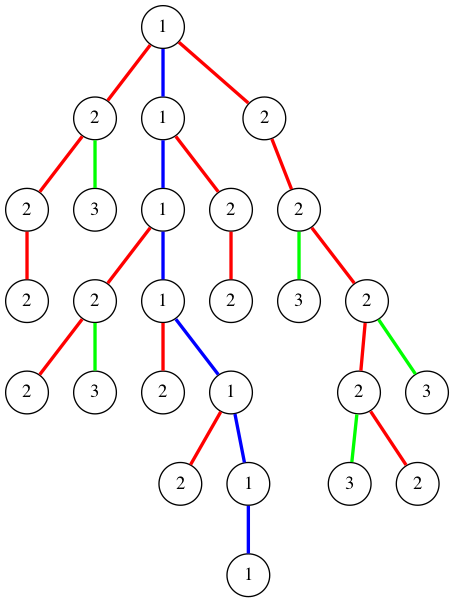
(b) Blue edges are level 1, red edges are level 2 and green edges are level 3.

Figure 1: An example of a tree before and after applying labels to nodes

3.6.1 Creating a new tree

Given a tree $T$, we can use Lemma 5 to decompose the tree into edge-disjoint paths. Next, we describe an algorithm to modify the tree recursively into a low height tree. The first step is to look at all the paths in $L_{1}$. $L_{1}$ is a special case since there is only one path in $L_{1}$ which goes from the depot to a leaf node. All the other levels $L_{i}$ could have multiple disjoint paths. Let $P$ be the path in $L_{1}$ and let $l(P)$ be the number of edges in path $P$. If $l(P)\leq\frac{\delta\log n}{\epsilon}$ for a $\delta>0$ to be specified, then we are done for $L_{1}$.

However, if $l(P)>\frac{\delta\log n}{\epsilon}$, we will compress the path into a low height one. We will do a sequence of what is called up-pushes. We will pick $s\leq\frac{\delta\log l(P)}{\epsilon}$ points to be anchor points. Let us call the anchor points $a_{1},\ldots,a_{s}$ where $a_{1}$ is the anchor point closest to the root and $a_{s}$ is closest to the leaf. We will later show how to find these anchor points.

Figure 2: A tree before an up-push (left) and after (right) with reduced height. The blue edge connecting $a_{i}$ and $a_{i+1}$ has weight $w=w_{p}+w_{q}+w_{s}+w_{t}$

Each up-push acts on nodes in $P$ between two consecutive anchor points $a_{i},a_{i+1}$ of the path $P$. During an up-push, we take all nodes in $P$ that lie between $a_{i}$ and $a_{i+1}$, which we will call $P^{\prime}$, and make each node in $P^{\prime}$ a child of $a_{i}$ with the edge connecting them to $a_{i}$ having weight 0. Suppose there is a child subtree $T_{j}$, which is a child of a node in $P^{\prime}$ with edge connection cost $w_{j}$, the subtree $T_{j}$ will become a child of $a_{i}$ with the edge connecting them having cost $w_{j}$ (see Figure 2). Once we have completed up-pushes for all paths in $L_{1}$, we will find anchor points and perform up-pushes for each path in $L_{2}$. We will repeat this for paths in $L_{i}$ after our algorithm has finished up-pushes for paths in $L_{i-1}$.

We will now describe how we can find the anchor points. We will first describe what we would like to achieve from anchor points. We want the cost associated with a path in $L_{i}$ for some tour to differ by at most $O(\epsilon)$ in our new tree compared to the the original tree. Suppose $P$ is a path in $L_{i}$ and a tour $t$ is travelling $P$ down to node $u$ which is between $a_{i}$ and $a_{i+1}$. Then the cost of the portion of the tour from root of $P$ to $a_{i}$ is the same in the original tree and the new tree; however the cost to travel from $a_{i}$ to $u$ is zero. We would like this cost in the original tree to be a small factor of the cost from the root of $P$ to $a_{i}$.

Our algorithm works as follows from top to bottom. For any path $P$ in $L_{i}$, we will set the top node of the path to be $a_{1}$ and its child in $P$ to be $a_{2}$. Our goal is to pick $a_{i}$ and $a_{i+1}$ for $i>2$ such that $w(a_{i},a_{i+1})>\epsilon\cdot w(a_{1},a_{i})$ and $w(a_{i},v)\leq\epsilon\cdot w(a_{1},a_{i})$ where $v$ is the last vertex on $a_{i},a_{i+1}$ path before $a_{i+1}$. If there is no $a_{i+1}$ such that $w(a_{i},a_{i+1})>\epsilon\cdot w(a_{1},a_{i})$, then we set the last node of $P$ to be $a_{i+1}$. So, we pick $a_{i+1}$ to be the farthest vertex from $a_{i}$ in $P$ such that $w(a_{i},v)\leq\epsilon\cdot w(a_{1},a_{i})$ where $v$ is the last node before $a_{i+1}$. This in turn would imply that $w(a_{1},a_{i+1})>(1+\epsilon)w(a_{1},a_{i})$, except if $a_{i+1}$ is the last node of the path. Hence, $w(a_{1},a_{i})>(1+\epsilon)^{i-2}w(a_{1},a_{2})>(1+\epsilon)^{i-2}$. Since edge weights are at most $2n^{3}/\epsilon^{2}$, the number of anchor points are at most $\frac{\delta\log n}{\epsilon}$ for some constant $\delta>0$

3.6.2 Analysis

In the last section, we showed that every path in some level $L_{i}$ can be made to have at most $O\left(\frac{\log n}{\epsilon}\right)$ nodes.

Lemma 6

The height of the new tree is $O\left(\frac{\log^{2}n}{\epsilon}\right)$.

Proof. In our algorithm, we first decomposed the tree into a set of edge-disjoint paths. The decomposition guarantees that one would first visit a lower level node in any root-toeaf path before visiting one with a higher level. Since there are at most $O(\log n)$ different levels, any root-to-leaf path will be a disjoint union of paths from levels $L_{1},\ldots,L_{s}$ and there can be at most one path from each level. Since the height of a path in any level, $L_{i}$ is at most $O\left(\frac{\log n}{\epsilon}\right)$, and there are at most $O(\log n)$ different levels, the maximum height in our new tree is at most $O\left(\frac{\log^{2}n}{\epsilon}\right)$  

Suppose we take a path $P$ at some level $L_{c}$. Let us fix a tour in an optimal solution and let the farthest point in $P$ the tour travels to be between anchor points [$a_{i}$,$a_{i+1}$). We use [$a_{i}$,$a_{i+1}$) denote that the tour crosses $a_{i}$ but will not cross $a_{i+1}$. Let $T$ be the original tree and let $T^{\prime}$ be the new tree with reduced height. A tour in the optimal solution for $T^{\prime}$ can visit nodes lying between $a_{i}$ and $a_{i+i}$ at no additional cost after visiting $a_{i}$. Suppose the cost of traversing the edges of $P$ in $T^{\prime}$ is denoted by $d$, then the cost of traversing the edges of $P$ in $T$ is going to be at most $(1+O(\epsilon))d$. This is because the cost of the edges between $a_{i}$ and the vertex before $a_{i+1}$ sum to at most $O(\epsilon)w(r,a_{i})$. Hence, the additional cost to cover them in $T$ is only going to be at most an $\epsilon$ fraction more.

Lemma 7

Let $T$ be the original tree, $T^{\prime}$ be the new tree, opt be the cost of the optimal set of tours covering $T$ and $\mbox{\sc opt}^{\prime}$ be the cost of the optimal set of tours covering $T^{\prime}$. Then,

$$\mbox{\sc opt}^{\prime}\leq\mbox{\sc opt}\leq(1+\epsilon)\mbox{\sc opt}^{\prime}.$$

Proof. Let us fix an optimal set of tours covering tree $T$ with cost opt. Suppose we pick a tour $t$ and decompose this tour into paths each of which is entirely within one level $L_{i}$. Suppose $P$ is a path of $t$ in some level $L_{c}$. Let the farthest point in $P$ the tour travels to be between anchor points [$a_{i}$,$a_{i+1}$). In our construction, the cost to visit any point lying between the root of $P$ and $a_{i}$ is the same in both $T$ and $T^{\prime}$. However, in $T^{\prime}$, the tour can visit any node lying between $a_{i}$ and $a_{i+1}$ for free, but the tour would have an additional cost to traverse these edges in tree $T$. Hence, for any path such $P$, the cost of a tour $t$ to traverse edges in $P$ is less in $T^{\prime}$ compared to $T$. Since any tour costs no more in instance $T^{\prime}$, we have $\mbox{\sc opt}^{\prime}\leq\mbox{\sc opt}$.

Conversely, the extra cost of covering points lying between $a_{i}$ and $a_{i+1}$ in $T$ is at most $O(\epsilon)$ times the cost of path $P$ (based on the property of anchor points). So the cost of using a path like $P$ is at most an $\epsilon$ factor more in $T$ compared to $T^{\prime}$. Thus, the cost of any tour $t$ in $T$ is at most $1+\epsilon$ times the cost of the same tour in $T^{\prime}$ and hence $\mbox{\sc opt}\leq(1+\epsilon)\mbox{\sc opt}^{\prime}$  

Instead of $T$, we can solve the instance on $T^{\prime}$ with height $O(\log^{2}n/\epsilon)$ and lift the solution for $T^{\prime}$ back to a solution for $T$. We obtain a solution for $T$ with cost at most $(1+\epsilon)\mbox{\sc opt}$.

4 QPTAS for Bounded Treewidth Graphs

Given a graph $G=(V,E)$ with treewidth $k$, we will assume we are given a tree decomposition $T=(V^{\prime},E^{\prime})$. We will refer to $G$ as the graph and $T$ as the tree. We will refer to vertices in $V$ by nodes and vertices in $V^{\prime}$ by bags. We will refer to edges in $E$ by edges and edges in $E^{\prime}$ by superedges.

Definition 5

A tree decomposition of a graph $G$ is a pair $(T,\{B_{t}\}_{t\in V(T)})$, where $T$ is a tree whose every node $t\in V^{\prime}$ is assigned a vertex subset $B_{t}\subseteq V(G)$, called a bag, such that the following three conditions hold:

1. $\cup_{t\in V(T)}B_{t}=V(G)$. In other words, every vertex of $G$ is in at least one bag.

2. For every $uv\in E(G)$, there exists a node $t$ of $T$ such that bag $B_{t}$ contains both $u$ and $v$.

3. For every $u\in V(G)$, the set $T_{u}=\{t\in V(T):u\in B_{t}\}$, i.e., the set of nodes whose corresponding bags contain $u$, induces a connected subtree of $T$.

For a bag $s$, let $C_{s}$ denote the union of nodes in bags below $s$ including $s$. Bag $s$ forms a boundary or border between nodes in $C_{s}$ and $V(G)\setminus C_{s}$. We will assume an arbitrary bag containing the depot to be root of the tree decomposition. Let $k$ be the treewidth of our graph $G$. We will assume that following properties hold for our tree decomposition $T$ of $G$ from the work of Boedlander and Hagerup [11],

• $T$ is binary.

• $T$ has depth $O(\log n)$.

• The width of $T$ is at most $k^{\prime}=3k+2$.

To simplify notation, by replacing $k^{\prime}$ with $k$ we will assume $T$ has height $\delta\log n$ for some fixed $\delta>0$ and each bag has width $k$. From the third property of a tree decomposition, we know that for every $u\in V(G)$, the set $T_{u}=\{t\in V(T):u\in X_{t}\}$ i.e., the set of nodes whose corresponding bags contain $u$, induces a connected subtree of $T$. Since the bags associated with a node $u\in V(G)$ correspond to a subtree in $T$, we will place the demand/tokens of $u$ at the root bag of the tree $T_{u}$ i.e. the bag containing $u$ closest to the root bag of $T$. Since $T_{u}$ is a tree, we are guaranteed a unique root bag of $T_{u}$ exists. We are doing this to ensure that the demand of a client is delivered exactly once.

Similar to how we showed the existence of a near-optimum solution for trees, we will modify the optimum solution OPT in a bottom-up manner by modifying the tours covering the set of nodes below bag $s$, $C_{s}$. For each bag $s$, we change the structure of the partial tours going down $C_{s}$ (by adding a few extra tours from the depot) and also adding some extra tokens for nodes in bag $s$ so that the partial tours that visit $C_{s}$ all have a size from one of polyogarithmic many possible sizes (buckets) while increasing the number and the cost of the tours by a small factor. Note that although a node can be in different bags, its initial demand is in one bag and we might add extra tokens to copies of it in other bags.

Similar to the case of tree, we assume the bags of the tree decomposition are partitioned into levels $V_{1},\ldots,V_{h}$ where $V_{1}$ is the bag containing the depot and $h$ is the height of $T$. For every tour ${\cal T}$ and every level $\ell$, we can define the notion of top and bottom part similar to the case of trees. For every $C_{s}$, a tour ${\cal T}$ enters $C_{s}$ through bag $s$ using a node $x$ and exists through node $z$ where both $x$ and $z$ have to be in $s$. Note that $x$ and $z$ could be equal if the tour enters and exists $s$ using the same node. For a bag $s$, let $n_{s}^{x,z}$ be the number of partial tours covering nodes in $C_{s}$ that enter through $x$ and exit through $z$ in $s$. For each bag and entry/exit pair, we will define the notion of a small/big bucket similar to the case of trees. For a big bucket, we will place the $n_{s}^{x,z}$ tours (ordered by increasing size) into groups $G_{1}^{x,z,s},\ldots,G_{g}^{x,z,s}$ of equal sizes. Let $h_{i}^{s,x,z,\max}(h_{i}^{s,x,z,\min})$ refer to the maximum (minimum) size of the tours in $G^{x,z,s}_{i}$.

Similar to the case of trees, let $f$ be a mapping from a tour in $G_{i}^{x,z,s}$ to one in $G_{i-1}^{x,z,s}$. Now suppose we modify OPT to $\mbox{\sc OPT}^{\prime}$ in the following way: for each tour ${\cal T}$ that has a partial tour in $t\in G_{i}^{x,z,s}$, replace the bottom part of ${\cal T}$ entering through $x$ and exiting through $z$ in $s$ from $t$ to $f(t)$ (which is in $G_{i-1}^{x,z,s}$). The only problem is that those tokens in $C_{s}$ that were picked up by the partial tours in $G_{g}^{x,z,s}$ are not covered by any tours and like the case of trees, these are orphant tokens. For each tour ${\cal T}$ and its (new) partial tour $t\in G_{i}^{x,z,s}$, if we add $h_{i}^{{x,z,s},\max}-|t|$ extra tokens at $s$ to be picked up by $t$, then each partial tour has size exactly same as the maximum size of its group without violating the capacities. Similar to the case of trees, we will show that if $n_{s}^{x,z}$ is sufficiently large (at least polylogarithmic), then if we sample a small fraction of the tours of the optimum at random and add two copies of them (as extra tours), they can be used to cover the orphant tokens.

4.1 Changing OPT to a near-optimum structured solution

Similar to the structure theorem for trees, we will modify the optimal solution OPT to a near-optimum solution $\mbox{\sc OPT}^{\prime}$ having certain properties. We will start at the last level, and modify partial tours from OPT at level $\ell$ to obtain $\mbox{\sc OPT}_{\ell}$. We will then iteratively obtain $\mbox{\sc OPT}_{\ell-1}$ by modifying partial tours from $\mbox{\sc OPT}_{\ell}$ at level $\ell-1$, and iteratively do this for each level until we obtain $\mbox{\sc OPT}_{1}=\mbox{\sc OPT}^{\prime}$.

Definition 6

For a bag $s$, the $i$-th bucket, $b_{i}$, entering at $x$ and exiting at $z$ contains the number of tours of $\mbox{\sc OPT}_{\ell}$ having coverage between $[\sigma_{i},\sigma_{i+1})$ tokens in $C_{s}$ where $\sigma_{i}$ is the $i$-th threshold value. We will denote this by a entry/exit-bag-bucket configuration $(s,b_{i},x,z)$. Let $n_{s,i}^{x,z}$ be the number of tours in bucket $b_{i}$ entering through $x$ and exiting through $z$ in bag $s$.

Definition 7

An entry/exit-bag-bucket configuration $(s,b_{i},x,z)$ is small if $n_{s,i}^{x,z}$ is at most $\alpha\log^{2}n/\epsilon$ and is big otherwise, for a constant $\alpha\geq\max\{1,20\delta\}$.

Note that for any bag $s$ and entry/exit-bag-bucket configuration $(s,b_{i},x,z)$, if $(s,b_{i},x,z)$ is small, we do not modify the partial tours in it. However, if $(s,b_{i},x,z)$ is a big bucket, we create groups $G_{i,1}^{s,x,z},\ldots,G_{i,g}^{s,x,z}$ of equal sizes, for $g=(2\delta\log n)/\epsilon$; so $|G_{i,j}^{s,x,z}|=\lceil n_{s,i}^{x,z}/g\rceil$. We also consider a mapping $f$ (as before) which maps (in the same order) the tours $t\in G^{s,x,z}_{i,j}$ to the tours in $G^{s,x,z}_{i,j-1}$ for all $1<j\leq g$. Consider set ${\bf T}_{\ell}$ of all the tours ${\cal T}$ in $\mbox{\sc OPT}_{\ell}$ that visit a bag in one of the lower levels $V_{\geq\ell}$. Consider an arbitrary such tour ${\cal T}$ that has a partial tour $t$ in a big entry/exit-bag-bucket configuration $(s,b_{i},x,z)$, suppose $t$ belongs to group $G_{i,j}^{s,x,z}$. We replace $t$ with $f(t)$ in ${\cal T}$.

Now, add some extra tokens at $x$ to be picked up by ${\cal T}$ so that the size of the partial tour of ${\cal T}$ at $C_{s}$ is exactly $h_{i,j-1}^{s,x,z,\max}$. If we make this change for all tours ${\cal T}\in{\bf T}_{\ell}$, each partial tour of them at level $\ell$ that was in a group $j<g$ of a big entry/exit-bag-bucket configuration $(s,b_{i},x,z)$ is replaced with a smaller partial tour from group $j-1$ of the same big entry/exit-bag-bucket configuration; after adding extra tokens to $x$ at bag $s$ (if needed), the size is the maximum size from group $j-1$. The tokens that were picked by partial tours from $G_{i,g}^{s,x,z}$ for a big entry/exit-bag-bucket configuration $(s,b_{i},x,z)$ are now orphant. We are going to (randomly) select a subset of tours of OPT as "extra tours" and add them to $\mbox{\sc OPT}^{\prime}$ and modify them such that they cover all the tokens that are now orphant (i.e. those that were covered by partial tours of $G_{i,g}^{s,x,z}$ for all big entry/exit-bag-bucket configuration $(s,b_{i},x,z)$ at level $\ell$). Suppose we select each tour ${\cal T}$ of OPT with probability $\epsilon$. We make two copies of the extra tour and we designate both extra copies to bags at one of the levels $V_{\ell}$ that it visits with equal probability.

Lemma 8

The expected cost of extra tours selected is $2\epsilon\cdot\mbox{\sc opt}$.

Proof. Suppose $f^{+}(e)$ and $f^{-}(e)$ denote the number of tours traveling edge $e$ in each of the two directions. So the contribution of edge $e$ to the optimal solution is $2\cdot w(e)\cdot(f^{+}(e)+f^{-}(e))$; $\mbox{\sc opt}=\sum_{e\in E}w(e)\cdot(f^{+}(e)+f^{-}(e))$. Let $m^{+}(e)$ ($m^{-}(e)$) denote the number of sampled tours from the tours contributing to $f^{+}(e)$ ($f^{-}(e)$). Since we used two extra copies for each sampled tour, the number of extra tours for an edge $e$ is $2(m^{+}(e)+m^{-}(e))$. Let ${\cal T}_{e,1},\ldots,{\cal T}_{e,f^{+}(e)+f^{-}(e)}$ be the tours using $e$ in either directions. Like in the case of trees, it is possible for a tour to use edge $e$ in both directions. Let $Y_{e,i}$ be a random variable which is 1 if tour ${\cal T}_{e,i}$ is sampled and $0$ otherwise.

$$\mathbb{E}{\left[Y_{e,i}\right]}=\mathbb{P}{\left[{\cal T}_{e,i}\text{ is sampled}\right]}=\epsilon.$$

Let $m^{+}(e)+m^{-}(e)=Y_{e}=\sum_{i=1}^{f^{+}(e)+f^{-}(e)}Y_{e,i}$. By linearity of expectations, we have

$$\mathbb{E}{\left[m^{+}(e)+m^{-}(e)\right]}=\mathbb{E}{\left[Y_{e}\right]}=\sum_{i=1}^{f^{+}(e)+f^{-}(e)}\mathbb{E}{\left[Y_{e,i}\right]}=\sum_{i=1}^{f^{+}(e)+f^{-}(e)}\epsilon=\epsilon\cdot(f^{+}(e)+f^{-}(e)).$$

Summing up the extra cost over all edges, the expected cost of the extra tours is

$$2\sum_{e\in E}\mathbb{E}{\left[m^{in}(e)+m^{out}(e)\right]}=2\epsilon\cdot\sum_{e\in E}(f^{+}(e)+f^{-}(e))=2\epsilon\cdot\mbox{\sc opt}.$$

 

Therefore, we can assume that the expected cost of all extra tours added is at most $2\epsilon\cdot\mbox{\sc opt}$. Let $X_{\ell}$ be the set of extra tours designated to bags in level $\ell$. We assume we add $X_{\ell}$ when we are building $\mbox{\sc OPT}_{\ell}$ (it is only for the sake of analysis). For each bag $s\in V_{\ell}$ and entry/exit-bag-bucket configuration $(s,b_{i},x,z)$, let $X^{s,x,z}_{i}$ be those in $X_{\ell}$ whose partial tour in $C_{s}$ has a size in bucket $b_{i}$. Each extra tour in $X_{\ell}$ will not be picking any of the tokens in levels $V_{<\ell}$ (as they will be covered by the tours already in $\mbox{\sc OPT}_{\ell})$; they are used to cover the orphant tokens created by partial tours of $G_{i,g}^{s,x,z}$ for each big entry/exit-bag-bucket configuration $(s,b_{i},x,z)$ with $s\in V_{\ell}$; as described below.

Lemma 9

For each level $V_{\ell}$, each bag $s\in V_{\ell}$ and big entry/exit-bag-bucket configuration $(s,b_{i},x,z)$, w.h.p. $|X^{s,x,z}_{i}|\geq\frac{\epsilon^{2}}{\delta\log n}\cdot n_{s,i}^{x,z}$.

Proof. Suppose $(s,b_{i},x,z)$ is a big entry/exit-bag-bucket configuration at some level $V_{\ell}$. Let $p_{1},\ldots,p_{n_{s,i}^{x,z}}$ be the partial tours in the entry/exit-bag-bucket configuration $(s,b_{i},x,z)$. Let the tour in OPT corresponding to $p_{i}$ be ${\cal T}$. Two copies of tour $p_{i}$ are assigned to $b_{i}$ if both of the following events are true:

• Let $A_{i}$ be the event where tour ${\cal T}$ is sampled as an extra tour. Since each tour is sampled with probability $\epsilon$, we have $\mathbb{P}{\left[A_{i}\right]}=\epsilon$.

• Let $B_{i}$ be the event where tour ${\cal T}$ is assigned to level $\ell$. There are $h=\delta\log n$ many levels and since ${\cal T}$ (if sampled) is assigned to any one of its levels, $\mathbb{P}{\left[B_{i}\right]}\geq 1/h\geq 1/(\delta\log n)$.

Let $Y_{i}$ be a random variable which is 1 if $p_{i}$ is an extra tour in $(v,b_{i})$ and 0 otherwise.

$$\mathbb{E}{\left[Y_{i}\right]}=\mathbb{P}{\left[Y_{i}=1\right]}=\mathbb{P}{\left[A_{i}\land B_{i}\right]}=\mathbb{P}{\left[A_{i}\right]}\cdot\mathbb{P}{\left[B_{i}\right]}\geq\epsilon/(\delta\log n).$$

Let $Y^{s,x,z}_{i}=\sum_{i=1}^{n_{s,i}^{x,z}}Y_{i}$ be the random variable keeping track of the number of sampled tours in $(s,b_{i},x,z)$. The number of extra tours, $|X^{s,x,z}_{i}|=2Y^{s,x,z}_{i}$ since we add two copies of a sampled tour to $X^{s,x,z}_{i}$. By linearity of expectation, we have

$$\mathbb{E}{\left[|X^{s,x,z}_{i}|\right]}=2\mathbb{E}{\left[Y^{s,x,z}_{i}\right]}=2\sum_{i=1}^{n_{s,i}^{x,z}}\mathbb{E}{\left[Y_{i}\right]}\geq\frac{2\epsilon}{\delta\log n}\cdot n_{s,i}^{x,z}.$$

We want to show that $|X^{s,x,z}_{i}|\geq\frac{\mathbb{E}{\left[|X^{s,x,z}_{i}|\right]}}{2}\geq\frac{\epsilon}{\delta\log n}\cdot n_{s,i}^{x,z}$ with high probability over all vertex-bucket pairs.

Using Chernoff Bound with $\mu=\mathbb{E}{\left[|X^{s,x,z}_{i}|\right]}\geq\frac{2\epsilon^{2}}{\delta\log^{2}n}\cdot n_{s,i}^{x,z}\geq 24\log n$ since $n_{s,i}^{x,z}\geq\alpha\log^{2}n/\epsilon$ and $\alpha\geq 20\delta$.

$$\begin{split}\mathbb{P}{\left[|X^{s,x,z}_{i}|<\frac{\mathbb{E}{\left[|X^{s,x,z}_{i}|\right]}}{2}\right]}&\leq e^{-(5\log n)}=\frac{1}{n^{5}}\end{split}$$

Note that the above equation only shows the concentration bound for a single entry/exit-bag-bucket configuration. For a bag, there are $O(k^{2})$ many entry/exit pairs. There are $O(kn)$ bags and $\tau=O(\log n/\epsilon)$ buckets, so the total number of entry/exit-bag-bucket configuration is at most $O(k^{2}n\log n/\epsilon)$. Suppose we do a union bound over all buckets, we get

$$\sum_{\text{all }(s,b_{i},x,z)\text{ configurations}}\mathbb{P}{\left[|X^{s,x,z}_{i}|<\frac{\mathbb{E}{\left[|X^{s,x,z}_{i}|\right]}}{2}\right]}\leq\frac{1}{n}.$$

We showed that for every entry/exit-bag-bucket configuration $(s,b_{i},x,z)$, $|X^{s,x,z}_{i}|\geq\frac{\epsilon}{\delta\log n}n_{s,i}^{x,z}$ holds with high probability.  

Lemma 10

Consider all bags $s\in V_{\ell}$, big entry/exit-bag-bucket configuration $(s,b_{i},x,z)$ and the partial tours in $G_{i,g}^{s,x,z}$. We can modify the tours in $X^{s,x,z}_{i}$ (without increasing the cost) and adding some extra tokens at nodes in $s$ (if needed) so that:

1. The tokens picked up by partial tours in $G_{i,g}^{s,x,z}$ are covered by some tour in $X^{s,x,z}_{i}$, and

2. The new partial tours that pick up the orphant tokens in $G_{i,g}^{s,x,z}$ have size exactly $h_{i,g}^{s,x,z,\max}$ and all tours still have size at most $Q$.

3. For each (new) partial tour of $X^{s,x,z}_{i}$ and every level $\ell^{\prime}>\ell$, the size of partial tours of $X^{s,x,z}_{i}$ at a bag $s^{\prime}$ at level $\ell^{\prime}$ is also one of $O((\log Q\log^{2}n)/\epsilon^{2})$ many possible sizes.

Proof. Our proof is going to be very similar to Lemma 4 for the case of trees. Our goal is to use the extra tours in $X^{s,x,z}_{i}$ to cover tokens picked up by partial tours of $G_{i,g}^{s,x,z}$ and we want each extra tour in $X^{s,x,z}_{i}$ to cover exactly $h_{i,g}^{s,x,z,\max}$ tokens. The tours in the last group, $G_{i,g}^{s,x,z}$, cover $\sum_{t\in G_{i,g}^{s,x,z}}|t|$ many tokens. We will add $\sum_{t\in G_{i,g}^{s,x,z}}(h_{i,g}^{s,x,z,\max}-|t|)$ extra tokens in node $x$ at bag $s$ for each entry/exit-bag-bucket configuration $(s,b_{i},x,z)$ so that there are $h_{i,g}^{s,x,z,\max}$ tokens corresponding to each partial tour in $G_{i,g}^{s,x,z}$. From now on, we will assume each partial tour in a last group $G_{i,g}^{s,x,z}$ covers $h_{i,g}^{s,x,z,\max}$ tokens.

Using Lemma 9, we know with high probability that $|X^{s,x,z}_{i}|/|G_{i,g}^{s,x,z}|\geq 2$ since $|X^{s,x,z}_{i}|\geq\frac{\epsilon}{\delta\log n}\cdot n_{s,i}^{x,z}=2|G_{i,g}^{s,x,z}|$. Let $Y^{s,x,z}_{i}$ denote the number of tours in entry/exit-bag-bucket configuration $(s,b_{i},x,z)$ that were sampled, so $|X^{s,x,z}_{i}|=2|Y^{s,x,z}_{i}|$ and $|Y^{s,x,z}_{i}|\geq|G_{i,g}^{s,x,z}|$ with high probability. We will start by creating a one-to-one mapping $s:G_{i,g}^{s,x,z}\rightarrow Y^{s,x,z}_{i}$ which maps each tour in $G_{i,g}^{s,x,z}$ to a sampled tour in $Y^{s,x,z}_{i}$. We know such a one-to-one mapping exists since $|Y^{s,x,z}_{i}|\geq|G_{i,g}^{s,x,z}|$.

Let ${\cal T}$ be a sampled tour in $Y^{s,x,z}_{i}$ with two extra copies of it, ${\cal T}_{1}$ and ${\cal T}_{2}$ in $X^{s,x,z}_{i}$. Let the partial tours of ${\cal T}$ at the bottom part in $V_{\ell}$ be $p_{1},\ldots,p_{m}$. We know $|{\cal T}|\geq\sum_{i=1}^{m}|p_{i}|$. Like the case for trees, $s$ maps at most one tour in $G_{i,g}^{s,x,z}$ to each $p_{j}$. If a tour from $G_{i,g}^{s,x,z}$ maps to $p_{j}$, we will assume the load assigned to $p_{j}$ would be $r_{j}=h_{i,g}^{s,x,z,\max}$ and $p_{j}$ has load 0 if no tour is assigned to it.

Suppose we think of $r_{1},\ldots,r_{m}$ as items and ${\cal T}_{1}$ and ${\cal T}_{2}$ as bins of size $Q$. We might not be able to fit all items $r_{1},\ldots,r_{m}$ into a bin of size $Q$ because $\sum_{i=1}^{m}|r_{i}|\leq(1+\epsilon)\sum_{i=1}^{m}|p_{i}|\leq(1+\epsilon)|{\cal T}|\leq(1+\epsilon)Q$. Similar to the case of trees, we can show that we can assign $r_{1},\ldots,r_{j}$ (for the maximum $j$) to ${\cal T}_{1}$ such that $\sum_{i=1}^{j}|r_{i}|\leq Q$ and the rest, $r_{j+1},\ldots,r_{m}$ to ${\cal T}_{2}$ such that both ${\cal T}_{1}$ and ${\cal T}_{2}$ cover at most $Q$ tokens and all items $r_{1},\ldots,r_{m}$ are covered by either ${\cal T}_{1}$ or ${\cal T}_{2}$. Hence, we have shown that the extra partial tours pick up exactly $h_{i,g}^{s,x,z,\max}$ while picking up orphant tokens from $G_{i,g}^{s,x,z}$.

Also, the size of the extra tours after this modification at each bag $s^{\prime}$ at any level $\ell^{\prime}>\ell$ is essentially the same as what each of $r_{i}$’s were at those levels and since we go bottom to top in the tree, each of those partial tours $r_{i}$ have a size that either belongs to a small bucket (and hence has one of $\alpha\log^{2}n/\epsilon$ many sizes) or a big entry/exit-bag bucket (and hence has one of $O((\log Q\log n)/\epsilon^{2})$ many sizes). Therefore, the size of partial tours of $X^{s,x,z}_{i}$ at any bag $s^{\prime}$ at level $\ell^{\prime}>\ell$ is one of $O((\log Q\log^{2}n)/\epsilon^{2})$ many sizes.  

Therefore, using Lemma 10, all the tokens of $C_{s}$ remain covered by partial tours; those partial tours in $G_{i,j}^{s,x,z}$ (for $1\leq j<g$) are tied to the top parts of the tours from group $G_{i,j+1}^{s,x,z}$ and the partial tours of $G_{i,g}^{s,x,z}$ will be tied to extra tours designated to level $\ell$. We also add extra tokens at nodes in $s$ to be picked up by the partial tours of $C_{s}$ so that each partial tour has a size exactly equal to the maximum size of a group. All in all, the extra cost paid to build $\mbox{\sc OPT}_{\ell}$ (from $\mbox{\sc OPT}_{\ell+1}$) is for the extra tours designated to level $\ell$.

Theorem 7

(Structure Theorem) Let opt be the cost of the optimal solution to instance ${\cal I}$. We can build an instance ${\cal I}^{\prime}$ such that each node has $\geq 1$ tokens and there exists a near-optimal solution $\mbox{\sc OPT}^{\prime}$ for ${\cal I}^{\prime}$ having expected cost $(1+2\epsilon)\mbox{\sc opt}$ with the following property. The partial tours going down $C_{s}$ for every bag $s$ in $\mbox{\sc OPT}^{\prime}$ has one of $O((\log Q\log^{2}n)/\epsilon^{2})$ possible sizes. More specifically, suppose $(s,b_{i},x,z)$ is a entry/exit-bag-bucket configuration for $\mbox{\sc OPT}^{\prime}$. Then either:

• $b_{i}$ is a small bucket and hence there are at most $\alpha\log^{2}n/\epsilon$ many partial tours of $C_{s}$ whose size is in bucket $b_{i}$, or

• $b_{i}$ is a big bucket; in this case there are $g=(2\delta\log n)/\epsilon$ many group sizes in $b_{i}$: $\sigma_{i}\leq h_{i,1}^{s,x,z,max}\leq\ldots\leq h_{i,g}^{s,x,z,max}<\sigma_{i+1}$ and every tour of bucket $i$ has one of these sizes.

Proof. We will show how to modify OPT to a near-optimal solution $\mbox{\sc OPT}^{\prime}$. We start from $\ell=h$ and let $\mbox{\sc OPT}_{\ell}=\mbox{\sc OPT}$. For decreasing values of $\ell$ we show, for each $\ell$ how to modify $\mbox{\sc OPT}_{\ell+1}$ to obtain $\mbox{\sc OPT}_{\ell}$. We do this in the following manner: we do not modify partial tours in small entry/exit-bag-bucket configuration. However, for tours in big entry/exit-bag-bucket configuration $(s,b_{i},x,z)$ in level $\ell-1$, we place them into $g$ groups $G_{i,1}^{s,x,z},\ldots,G_{i,g}^{s,x,z}$ of equal sizes by placing the $i$’th $n_{s,i}^{x,z}/g$ partial tours into $G_{i,j}^{s,x,z}$. We have a mapping $f$ from each partial tour in $G_{i,j-1}^{s,x,z}$ to one in $G_{i,j}^{s,x,z}$ for $j\in\{2,\ldots,g\}$. We modify $\mbox{\sc OPT}_{\ell}$ to $\mbox{\sc OPT}_{l+1}$ in the following way: for each tour ${\cal T}$ that has a partial tour $t\in G_{i,j}^{s,x,z}$, replace the bottom part of ${\cal T}$ at $s$ from $t$ to $f(t)$ (which is in $G_{i,j-1}^{s,x,z}$). For each tour $t\in G_{i,j-1}^{s,x,z}$, we will add $h_{i,j-1}^{s,x,z,\max}-|t|$ many extra tokens at $x$ in $s$. Note that by this change, the size of any tour such as ${\cal T}$ can only decrease and we are not violating feasibility of the tour because $h_{i,j-1}^{s,x,z,\max}\leq h_{i,j}^{s,x,z,\min}$. However, the tokens in $C_{s}$ picked up by the partial tours in $G_{i,g}^{s,x,z}$ are not covered by any tours. We can use Lemma 10 to show how we can use extra tours to cover the partial tours in $G_{i,g}^{s,x,z}$ such that the new partial tours have size exactly $h_{i,g}^{s,x,z,\max}$.

We will inductively repeat this for levels $\ell-2,\ell-3,\ldots,1$ and obtain $\mbox{\sc OPT}_{1}=\mbox{\sc OPT}^{\prime}$. Note that by adding extra tokens $h_{i,j-1}^{s,x,z,\max}-|t|$ for a tour $t\in G_{i,j-1}^{s,x,z}$, we are enforcing that the coverage of each tour is the maximum size of tours in its group. In a big bucket, there are $g=(2\delta\log n)/\epsilon$ many group sizes, so there are $O(\log n/\epsilon)$ possible sizes for tours in big entry/exit-bag-bucket configuration at a node. In a small entry/exit-bag-bucket configuration, there can be at most $\alpha\log^{2}n/\epsilon$ many tours and since there are $\tau=O(\log Q/\epsilon)$ many buckets, there can be at most $O((\log Q\log^{2}n)/\epsilon^{2})$ many tour sizes covering $C_{b}$.

Using Lemma 8, we know the expected cost of the extra tours is at most $2\epsilon\cdot\mbox{\sc opt}$, so the expected cost of $\mbox{\sc opt}^{\prime}\leq(1+2\epsilon)\mbox{\sc opt}$.  

4.2 Dynamic Program

In this section we prove Theorem 2 by presenting a dynamic program that will compute a near optimum solution guaranteed by the structure theorem (Theorem 7). For a given bag $s$, we will estimate the number of tours entering and exiting $s$. Informally, we will have a vector $\vec{n}^{s,x,z}\in[n]^{\tau}$ where if $i<1/\epsilon$, $\vec{n}_{i}^{s,x,z}$ keeps track of the exact number of tours covering $i$ tokens in $C_{s}$ by entering through $x$ and exiting though $z$ and if $i\geq 1/\epsilon$, $\vec{n}_{i}^{s,x,z}$ keeps track of the number of tours covering between $[\sigma_{i},\sigma_{i+1})$ tokens. Let $a_{s}$ denote the total number of tokens to be picked up from nodes from bags below and including bag $s$. Since each bag $s$ has $k$ nodes, we use $\vec{o}_{s}\in[n]^{k}$ to denote the extra tokens to be picked up from nodes at bag $s$. If $v$ is a node in bag $s$, then $\vec{o}_{s,v}$ denotes the number of extra tokens to be picked up at $v$ in $s$. For a given entry/exit-bag-bucket configuration $(s,b_{i},x,z)$, we will keep track of other pieces of information conditional on whether it is small or big. If entry/exit-bag-bucket configuration $(s,b_{i},x,z)$ is small, we will store all tour sizes exactly. Since the number of tours in a small entry/exit-bag-bucket configuration is at most $\gamma=\alpha\log^{2}n/\epsilon$, we will use a vector $\vec{t}^{s,x,z,i}\in[n]^{\gamma}$ to represent the tours where $\vec{t}^{s,x,z,i}_{j}$ represents the size of the $j$-th tour in the $i$-th bucket of tours covering $C_{s}$ entering through $x$ and exiting through $z$.

If the entry/exit-bag-bucket configuration $(s,b_{i},x,z)$ is big, there are $g=(2\delta\log n)/\epsilon$ many tour sizes corresponding to $n^{O(g)}$ possibilities. For each entry/exit-bag-bucket configuration $(s,b_{i},x,z)$, we need to keep track of the following information,

• $\vec{h}^{s,x,z,i}\in[n]^{g}$ is a vector where $\vec{h}^{s,x,z,i}_{j}=h_{i,j}^{s,x,z,\max}$, which is the size of the maximum tour which lies in group $G_{i,j}^{s,x,z}$ of bucket $i$ at bag $s$ entering through $x$ and exiting through $z$.

• $\vec{l}^{s,x,z,i}\in[n]^{g}$ is a vector where $\vec{l}^{s,x,z,i}_{j}$ denotes the number of partial tours covering $h_{i,j}^{s,x,z,\max}$ tokens which lies in group $G_{i,j}^{s,x,z}$ of bucket $i$ at bag $s$ entering through $x$ and exiting through $z$.

For a bag $s$ and entry/exit pairs, let $\vec{p}_{s,x,z}$ be a vector containing information about all tours entering and exiting $s$ through $x$ and $z$ across all buckets.

$$\vec{p}_{s,x,z}=[\vec{n}^{s,x,z},(\vec{t}^{s,x,z,1},\vec{h}^{s,x,z,1},\vec{l}^{s,x,z,1}),(\vec{t}^{s,x,z,2},\vec{h}^{s,x,z,2},\vec{l}^{s,x,z,2}),\ldots,(\vec{t}^{s,x,z,\tau},\vec{h}^{s,x,z,\tau},\vec{l}^{s,x,z,\tau})].$$

Similar to the case of trees, an entry/exit-bag-bucket configuration $(s,b_{i},x,z)$ is either small or big and cannot be both, hence given $(\vec{t}^{s,x,z,i},\vec{h}^{s,x,z,i},\vec{l}^{s,x,z,i})$, it cannot be the case that $\vec{t}^{s,x,z,i}\neq\vec{0},\vec{h}^{s,x,z,i}\neq\vec{0}$ and $\vec{l}^{s,x,z,i}\neq\vec{0}$. Since a bag $s$ contains $O(k)$ nodes, then we will let $\vec{y}_{s}$ denote a configuration of all partial tours covering tokens in $C_{s}$ which are entering and exiting $s$. Let $v_{1},\ldots,v_{d}$ be the set of all nodes in $s$, then $\vec{y}_{s}$ contains information of tours entering and exiting $s$ through pairs of nodes in $\{v_{1},\ldots,v_{d}\}$. Note that a tour can enter and exit $s$ through the same node.

$$\vec{y}_{s}=[a_{s},\vec{o}_{s},\vec{p}_{s,v_{1},v_{1}},\vec{p}_{s,v_{1},v_{2}},\ldots,\vec{p}_{s,v_{d},v_{d-1}},\vec{p}_{s,v_{d},v_{d}}].$$

The subproblem $\textbf{A}[s,\vec{y}_{s}]$ is supposed to be the minimum cost collection of partial tours covering $C_{s}$ having tour profiles corresponding to $\vec{y}_{s}$. Our dynamic program heavily relies on the properties of the near-optimal solution characterized by the structure theorem. We will compute $\textbf{A}[\cdot,\cdot]$ in a bottom-up manner, computing $\textbf{A}[s,\vec{y}_{s}]$ after we have computed entries for the children bags of $s$.

The final answer is obtained by looking at various entries of the root bag of the tree decomposition, denoted by $r_{s}$. We will take the minimum cost entry amongst $\textbf{A}[r_{s},\vec{y}_{r_{s}}]$ such that $\vec{y}_{r_{s}}$ is the configuration where all tours enter and exit $r_{s}$ only through the depot, $r$. We will compute our solution in a bottom-up manner.

For any nodes $u,v$ in bag $s$, if there is no edge between $u$ and $v$, we can add an edge between them and the cost of the edge is the shortest path cost between $u$ and $v$ in $G$. Similarly, for two adjacent bags, $s$ and $s_{1}$, if $u\in s$ and $v\in s_{1}$ and if there is no edge between $u$ and $v$ in $G$, we will add an edge between them and the cost of the edge is the shortest path cost between $u$ and $v$ in $G$. If $u=v$, then the cost of the edge connecting them can be assumed to be zero. Let $\left\lVert\vec{o}_{s}\right\rVert=\sum_{u\in s}\vec{o}_{s,u}$.

For the base case, we consider leaf bags. A leaf bag $s$ could have $a_{s}\geq 1$ tokens where $a_{s}=\left\lVert\vec{o}_{s}\right\rVert$. We will defer how we compute $\textbf{A}[s,\vec{y}_{s}]$ to the end of this section. Informally, we will set $\textbf{A}[s,\vec{y}_{s}]$ to be the minimum cost of the edges between nodes in bag $s$ used for the tours in $\vec{y}_{s}$ to pick up $\vec{o}_{s}$ tokens located at nodes in bag $s$. The total capacity of the tours in $\vec{y}_{s}$ should be exactly $a_{s}$ and a token at a node should be picked up by one of the tours in $\vec{y}_{s}$. From our structure theorem, we know there exists a near optimum solution such that each partial tour has one of $O(\log Q\log^{2}n/\epsilon^{2})$ tour sizes and for each small bucket, there are at most $\alpha\log^{2}n/\epsilon$ partial tours in it. For every big bucket, there are $g=(2\delta\log n)/\epsilon$ many group sizes and every tour of bucket $i$ has one of those sizes. We are computing all possible $\textbf{A}[s,\vec{y}_{s}]$ entries and from our structure theorem, we know one of them has near-optimum expected cost, so by enumerating all possibilities, our dynamic program finds a near-optimums solution for the leaf bag, proving the base case.

Recall that the tree $T$ is binary. Suppose bag $s$ has two children in $T$, $s_{1}$ and $s_{2}$. To compute cell $\textbf{A}[s,\vec{y}_{s}]$, we will use the entries of its children, $\textbf{A}[s_{1},\vec{y}^{\prime}]$ and $\textbf{A}[s_{2},\vec{y}^{\prime\prime}]$. Suppose $C_{s_{i}}$ has $a_{s_{i}}$ tokens, then $a_{s}=\left\lVert\vec{o}_{s}\right\rVert+a_{s_{1}}+a_{s_{2}}$. $\textbf{H}[\vec{o}_{s},\vec{y}_{s},\vec{y}^{\prime},\vec{y}^{\prime\prime}]$ checks whether the tour profiles $\vec{y}_{s},\vec{y}^{\prime}$ and $\vec{y}^{\prime\prime}$ are consistent meaning that all tokens picked up by tours in $\vec{y}^{\prime}$ and $\vec{y}^{\prime\prime}$ along with tokens in $s$, $\vec{o}_{s}$ are picked up by tours in $\vec{y}_{s}$. We will also define $\textbf{I}[\cdot,\cdot,\cdot,\cdot]$ where $\textbf{I}[\vec{o}_{s},\vec{y}_{s},\vec{y}^{\prime},\vec{y}^{\prime\prime}]$ denotes the cost of using the edges in bag $s$, edges connecting nodes in $s$ and $s_{1}$, and edges connecting nodes in $s$ and $s_{2}$. We can think of I as the cost of using edges to patch up partial tours covering $C_{s_{1}}$ and partial tours covering $C_{s_{2}}$ to create tours covering $C_{s}$. We will explain in the next section how H and I are computed. Recall $\vec{o}_{s}$ is part of $\vec{y}_{s}$. Suppose we have already computed the entries $\textbf{A}[s_{1},\cdot]$ and $\textbf{A}[s_{2},\cdot]$, we will compute $\textbf{A}[s,\cdot]$ in the following way:

$$\textbf{A}[s,\vec{y}_{s}]=\underset{\vec{y}^{\prime},\vec{y}^{\prime\prime}:\textbf{H}[\vec{o}_{s},\vec{y}_{s},\vec{y}^{\prime},\vec{y}^{\prime\prime}]=\text{True}}{\text{min }}\{\textbf{A}[s_{1},\vec{y}^{\prime}]+\textbf{A}[s_{2},\vec{y}^{\prime\prime}]+\textbf{I}[\vec{o}_{s},\vec{y}_{s},\vec{y}^{\prime},\vec{y}^{\prime\prime}]\}.$$

There are four possibilities for each partial tour $t$ at bag $s$ going down $C_{s}$ covering tokens for the subtree rooted at children bags, $s_{1}$ and $s_{2}$ while also picking up extra tokens from nodes in $s$:

• $t$ could be a tour that picks up tokens from nodes at bag $s$ and does not visit or pick up tokens in $C_{s_{1}}\cup C_{s_{2}}$.

• $t$ could be a tour that picks up tokens from nodes at bag $s$ and picks up tokens only from $C_{s_{1}}$.

• $t$ could be a tour that picks up tokens from nodes at bag $s$ and picks up tokens only from $C_{s_{2}}$.

• $t$ could be a tour that picks up tokens from nodes at bag $s$ and picks up tokens from $C_{s_{1}}\cup C_{s_{2}}$.

We would find the minimum cost over all configurations $\vec{y}_{s},\vec{y}^{\prime},\vec{y}^{\prime\prime}$ as long as $\vec{y}_{s},\vec{y}^{\prime},\vec{y}^{\prime\prime}$ are consistent. We say $\vec{y}_{s},\vec{y}^{\prime},\vec{y}^{\prime\prime}$ are consistent if there is a way to write each tour in $\vec{y}_{s}$ as a combination of at most one tour from $\vec{y}^{\prime}$, at most one tour from $\vec{y}^{\prime\prime}$ while also picking up extra tokens from nodes in $s$. We would also require that all tokens in $\vec{y}^{\prime}$ and $\vec{y}^{\prime\prime}$ are picked up by tours in $\vec{y}_{s}$.

For a leaf bag $s$, $\textbf{I}[\vec{o}_{s},\vec{y}_{s},\vec{0},\vec{0}]$ denotes the minimum cost of tours entering bag $s$ and visiting the nodes in $s$ such that all tokens in $s$ are picked up by some tour in $\vec{y}_{s}$. The last two entries are set to $\vec{0}$ since $s$ is a leaf bag, and has no children, and there are no other tours (apart from those in $\vec{y}_{s}$) entering or exiting through nodes in bag $s$. We will set $\textbf{A}[s,\vec{y}_{s}]=\textbf{I}[\vec{o}_{s},\vec{y}_{s},\vec{0},\vec{0}]$ since $\textbf{I}[\vec{o}_{s},\vec{y}_{s},\vec{0},\vec{0}]$ computes exactly the minimum cost collection of partial tours covering $C_{s}=s$ having tour profiles corresponding to $\vec{y}_{s}$. We will explain how to compute the entries of $\textbf{I}[\cdot,\cdot,\cdot,\cdot]$ in the next section.

4.3 Checking Consistency

In our dynamic program, we are given three vectors $\vec{y}_{s},\vec{y}^{\prime},\vec{y}^{\prime\prime}$ where $s$ is a bag having child bags $s_{1}$ and $s_{2}$. $\vec{y}^{\prime}$ represents the configuration of tours covering $C_{s_{1}}$ and $\vec{y}^{\prime\prime}$ represents the configuration of tours covering $C_{s_{2}}$. Given a $\vec{y}_{s}$, for each node $u$ in $s$, there are $\vec{o}_{s,u}$ many tokens to be picked up at $u$. We require the tokens for nodes in $s$ and tokens covered by the partial tours from $\vec{y}^{\prime}$ and $\vec{y}^{\prime\prime}$ to be picked up by tours in $\vec{y}_{s}$. For simplicity, we will refer to a tour from $\vec{y}_{s}$ as $t_{s}$, $\vec{y}^{\prime}$ as $t_{u}$ and a tour from $\vec{y}^{\prime\prime}$ as $t_{w}$.

Definition 8

We say configurations $\vec{y}_{s},\vec{y}^{\prime}$ and $\vec{y}^{\prime\prime}$ are consistent if the following holds:

• Every tour in $\vec{y}^{\prime}$ maps to some tour in $\vec{y}_{s}$.

• Every tour in $\vec{y}^{\prime\prime}$ maps to some tour in $\vec{y}_{s}$.

• Every tour in $\vec{y}_{s}$ has at most two mapping to it and both cannot be from $\vec{y}^{\prime}$ or $\vec{y}^{\prime\prime}$.

• Suppose only one tour $t_{u}$ ($t_{w}$) maps to a tour $t_{s}$ in $\vec{y}_{s}$. The number of extra tokens (from nodes in $s$) in total picked up by tour $t_{s}$ from nodes in bag $s$ is exactly $|t_{s}|-|t_{u}|$ ($|t_{s}|-|t_{w}|$).

• Suppose $t_{s}$ has two tours: $t_{u}$ in $\vec{y}^{\prime}$ and $t_{w}$ in $\vec{y}^{\prime\prime}$ mapping to it, then the number of extra tokens (from nodes in $s$) picked up by tour $t_{s}$ at $s$ is exactly $|t_{s}|-|t_{u}|-|t_{w}|$.

• All tokens of nodes at bag $s$, $\vec{o}_{s}$ are picked up tours in $\vec{y}_{s}$.

Consistency ensures that we can patch up tours from subproblems and combine them into new tours in a correct manner while also picking up extra tokens from nodes in $s$. We will describe how we can compute consistency. Instead of using $\vec{y}_{s}$, we will use $\vec{z}_{s}$ which is the same as $\vec{y}_{s}$, but excludes information about the number of tokens in a bag, and only tracks information about the number of tours passing through bag $s$.

$$\vec{z}_{s}=[\vec{p}_{s,v_{1},v_{1}},\vec{p}_{s,v_{1},v_{2}},\ldots,\vec{p}_{s,v_{d},v_{d-1}},\vec{p}_{s,v_{d},v_{d}}].$$

We will similarly define $\vec{z}^{\prime}$ and $\vec{z}^{\prime\prime}$. Suppose $t_{s,x_{1},x_{2}}$ is a tour in $s$ which enters through $x_{1}$ and exits through $x_{2}$, let $\vec{z}_{s}-t_{s,x_{1},x_{2}}$ refers to the configuration $\vec{z}_{s}$ having one less tour of size $|t_{s,x_{1},x_{2}}|$ from tours entering through $x_{1}$ and exiting through $x_{2}$ in $s$. Recall that $\vec{o}_{s}$ is the vector of extra tokens at each node in bag $s$ which need to be covered by tours in $\vec{z}_{s}$.

Given $\vec{z}_{s},\vec{z}^{\prime},\vec{z}^{\prime\prime}$ and $\vec{o}_{s}$, we will use the table H to check if $\vec{z}_{s},\vec{z}^{\prime},\vec{z}^{\prime\prime}$ are consistent. Let $\textbf{H}[\vec{o}_{s},\vec{z}_{s},\vec{z}^{\prime},\vec{z}^{\prime\prime}]=$True if $\vec{z}_{s},\vec{z}^{\prime}$ and $\vec{z}^{\prime\prime}$ are consistent and False otherwise. For the base case, $\textbf{H}[\vec{0},\vec{0},\vec{0},\vec{0}]=$True. For the recurrence, we will look at all possible ways of combining tours from $\vec{z}^{\prime}$ and $\vec{z}^{\prime\prime}$ into $\vec{z}_{s}$ while also picking up extra tokens from bag $s$. For a tour $t_{s}$, let $\vec{o}^{\prime}_{s,t_{s}}$ be a vector where $\vec{o}^{\prime}_{s,t_{s},u}$ denotes the number of extra tokens picked up by $t_{s}$ at node $u$ in bag $s$. Let $\left\lVert\vec{o}^{\prime}_{s,t_{s}}\right\rVert=\sum_{u\in s}\vec{o}^{\prime}_{s,t_{s},u}$ count the number of tokens picked up by $t_{s}$ from nodes in $s$.

Recall that a tour $t_{s}$ merges with at most one tour $t_{u}$ from $\vec{z}^{\prime}$ and at most one tour $t_{w}$ from $\vec{z}^{\prime\prime}$. Similar to the case of trees, we can write the recurrence of our consistency table as:

$$\textbf{H}[\vec{o}_{s},\vec{z}_{s},\vec{z}^{\prime},\vec{z}^{\prime\prime}]=\underset{\begin{subarray}{c}t_{s},t_{u},t_{w},\vec{o}^{\prime}_{s,t_{s}}\\ |t_{s}|=|t_{u}|+|t_{w}|+\left\lVert\vec{o}^{\prime}_{s,t_{s}}\right\rVert\end{subarray}}{\bigvee}\textbf{H}[\vec{o}_{s}-\vec{o}^{\prime}_{s,t_{s}},\vec{z}_{s}-t_{s},\vec{z}^{\prime}-t_{u},\vec{z}^{\prime\prime}-t_{w}].$$

Although the above DP lets us check if $\vec{y}_{s},\vec{y}^{\prime}$ and $\vec{y}^{\prime\prime}$ are consistent, the entries of H are True/False and does not give us information about the optimum order in which tour $t_{s}$ should visit nodes in $s$ or the cost associated with such an ordering. Suppose the tour $t_{s}$ visited $k_{s}$ nodes in bag $s$, there are $O(k^{k_{s}})$ many paths that tour $t_{s}$ can choose to take and each path has a cost associated with it. Our goal is to find a path having the smallest cost while also picking up tokens from nodes in bag $s$. We will next compute the minimum cost way to visit nodes in $s$ and pick up tokens from them. Recall the recurrence of our dynamic program for A is the following,

$$\textbf{A}[s,\vec{y}_{s}]=\underset{\vec{y}^{\prime},\vec{y}^{\prime\prime}:\textbf{H}[\vec{o}_{s},\vec{y}_{s},\vec{y}^{\prime},\vec{y}^{\prime\prime}]=\text{True}}{\text{min }}\{\textbf{A}[s_{1},\vec{y}^{\prime}]+\textbf{A}[s_{2},\vec{y}^{\prime\prime}]+\textbf{I}[\vec{o}_{s},\vec{y}_{s},\vec{y}^{\prime},\vec{y}^{\prime\prime}]\}.$$

The cost of using edges in $C_{s_{1}}$ and $C_{s_{2}}$ by the partial tours in $\vec{y}^{\prime}$ and $\vec{y}^{\prime\prime}$ in $\vec{y}_{s}$ are accounted for by $\textbf{A}[s_{1},\vec{y}^{\prime}]+\textbf{A}[s_{2},\vec{y}^{\prime\prime}]$. However, we have not accounted for the cost of hopping from one node to the other in $s$ and also the cost of going from nodes in $s$ to nodes in child bags, $s_{1}$ and $s_{2}$. Note that a tour $t_{s}$ enters and exits through each node in $s$ at most once. Note that a tour visits a node $u$ in $s$ if it either has to pick up tokens at $u$ or if it uses $u$ to enter the child bag. If a tour $t_{s}$ enters and exist a node two or more times, we can short cut it so that it enters and exits only once. A tour in $t_{s}$ can visit up to $k$ nodes in a bag $s$ and it could use one of the nodes to enter a child bag ($s_{1}$ or $s_{2}$) and if so, it would use a node in $s$ to return to the bag $s$. This means the tour $t_{s}$ could visit up to $k$ nodes in $s$. Let $P_{t_{s}}$ be the ordered collection of edges where either both endpoints are in $s$ or one endpoint is in $s$ and the other is in $s_{1}\cup s_{2}$. There are $O((3k)^{3k})$ possible permutations of for $P_{t_{s}}$ and $t_{s}$ could pick up at most $Q$ tokens from each node that it visits and each permutation has an associated cost with it. The number of possibilities for $P_{t_{s}}$ characterized by the the order of visiting nodes and the number of tokens picked up by tour $t_{s}$ from the $k$ nodes in bag $s$ is at most $O(Q^{k}(3k)^{3k})$. We will let $\text{cost}(P_{t_{s}})$ denote the cost of the edges in $P_{t_{s}}$. The following figure illustrates an example of one such tour $t_{s}$ (in red) and $P_{t_{s}}$ (in blue).

Figure 3: Blue edges represent one such edge set for a particular tour $t_{s}$

Although H tells us if $\vec{y}_{s},\vec{y}^{\prime}$ and $\vec{y}^{\prime\prime}$ are consistent, $\textbf{H}[\vec{o}_{s},\vec{z}_{s},\vec{z}^{\prime},\vec{z}^{\prime\prime}]$ does not give us the cost of patching up $\vec{y}^{\prime}$ and $\vec{y}^{\prime\prime}$ to form $\vec{y}_{s}$. We will use H to compute I. Let $\textbf{I}[\vec{o}_{s},\vec{z}_{s},\vec{z}^{\prime},\vec{z}^{\prime\prime}]$ denote the cost of using the edges in bag $s$, edges connecting nodes in $s$ and $s_{1}$, and edges connecting nodes in $s$ and $s_{2}$. We can think of I as the cost of using edges to patch up partial tours covering $C_{s_{1}}$, $\vec{z}^{\prime}$ and partial tours covering $C_{s_{2}}$, $\vec{z}^{\prime\prime}$, to create tours covering $C_{s}$, $\vec{z}_{s}$. For the base case, we will set $\textbf{I}[\vec{0},\vec{0},\vec{0},\vec{0}]=0$ and set all other entries to infinity. We will only compute an entry $\textbf{I}[\vec{o}_{s},\vec{z}_{s},\vec{z}^{\prime},\vec{z}^{\prime\prime}]$ if $\textbf{H}[\vec{o}_{s},\vec{z}_{s},\vec{z}^{\prime},\vec{z}^{\prime\prime}]=$True. Along with all possible values of $\vec{o}^{\prime}_{s},t_{s},t_{u},t_{w}$, we will also look at all possible paths $P_{t_{s}}$. In our recurrence, we are taking a tour $t_{s}$ from $\vec{y}_{s}$ along with maybe a tour $t_{u}$ from $\vec{y}^{\prime}$, maybe a tour $t_{w}$ from $\vec{y}^{\prime\prime}$ along with tokens $\vec{o}^{\prime}_{s}$ that $t_{s}$ covers at nodes in bag $s$. For such a tour $t_{s}$, there are $O(Q^{k}(3k)^{3k})$ many possibilities for $P_{t_{s}}$. For a fixed $P_{t_{s}}$, $\text{cost}(P_{t_{s}})$ is the cost of forming $t_{s}$ from patching up $t_{u}$ and $t_{w}$ while picking up extra tokens from nodes in $s$. We will enumerate through all possibilities, break the recurrence into subproblems and find a solution of minimum cost. We can write the recurrence as follows:

$$\textbf{I}[\vec{o}_{s},\vec{z}_{s},\vec{z}^{\prime},\vec{z}^{\prime\prime}]=\underset{\begin{subarray}{c}t_{s},t_{u},t_{w},P_{t_{s}},\vec{o}^{\prime}_{s,t_{s}}\\ |t_{s}|=|t_{u}|+|t_{w}|+\left\lVert\vec{o}^{\prime}_{s,t_{s}}\right\rVert\end{subarray}}{\text{min}}\left\{\text{cost}(P_{t_{s}})+\textbf{I}[\vec{o}_{s}-\vec{o}^{\prime}_{s,t_{s}},\vec{z}_{s}-t_{s},\vec{z}^{\prime}-t_{u},\vec{z}^{\prime\prime}-t_{w}]\right\}.$$

4.4 Time Complexity

We will work bottom-up and analyze the time complexity of $\textbf{A}[\cdot,\cdot]$ on the assumption that we have already precomputed our consistency table $\textbf{I}[\cdot,\cdot,\cdot,\cdot]$. Computing $\textbf{A}[s,\cdot]$ requires looking at entries of child bags in $\textbf{A}[\cdot,\cdot]$. Given $\vec{y}_{s},\vec{y}^{\prime}$ and $\vec{y}^{\prime\prime}$ which are consistent, computing the cost of $\textbf{A}[s,\vec{y}_{s}]$ takes $O(1)$ time. Each $\vec{y}_{s}$ consists of $O(k^{2})$ different $\vec{p}_{s,u,v}$ vectors. Each $\vec{p}_{s,u,v}$ contains $\tau$ many triples $(\vec{t}^{s,x,z,i},\vec{h}^{s,x,z,i},\vec{l}^{s,x,z,i})$.

1. Each $\vec{t}^{s,x,z,i}$ has $n^{O(\log^{2}n/\epsilon)}$ possibilities since there are at most $O(\log^{2}n/\epsilon)$ tours in a small bucket.

2. Each $\vec{h}^{s,x,z,i}$ and $\vec{l}^{s,x,z,i}$ have $n^{O(g)}$ possibilities. Recall that $g=(2\delta\log n)/\epsilon$, so each $\vec{h}^{s,x,z,i}$ and $\vec{l}^{s,x,z,i}$ have $n^{O(\log n/\epsilon)}$ possibilities.

3. Each triple $(\vec{t}^{s,x,z,i},\vec{h}^{s,x,z,i},\vec{l}^{s,x,z,i})$ has $n^{O(\log^{2}n/\epsilon)}$ possibilities.

4. Since $\vec{p}_{s,u,v}$ has $\tau=O(\log Q/\epsilon)$ many such triples, the number of possible entries for $\vec{p}_{s,u,v}$ is $n^{O(\tau\log^{2}n/\epsilon)}=n^{O(\log Q\log^{2}n/\epsilon^{2})}$.

5. Since $\vec{y}_{s}$ consists of $O(k^{2})$ different entries of $\vec{p}$, so the total number of possible entries for each $\vec{y}_{s}$ is $n^{O(k^{2}\log Q\log^{2}n/\epsilon^{2})}$.

Since there are $n^{O(k^{2}\log Q\log^{2}n/\epsilon^{2})}$ possibilities for $\vec{y}_{s},\vec{y}^{\prime}$ and $\vec{y}^{\prime\prime}$, the time of computing DP entries of $\textbf{A}[s,\cdot]$ for a single bag $s$ would take $n^{O(k^{2}\log Q\log^{2}n/\epsilon^{2})}$ and across all bags of the tree decomposition, it would still be $n^{O(k^{2}\log Q\log^{2}n/\epsilon^{2})}$.

Now, we will analyze the time of computing the consistency table $\textbf{I}[\cdot,\cdot,\cdot,\cdot]$. Assuming we have computed smaller entries, the cost of computing if $\textbf{I}[\vec{o}_{s},\vec{z}_{s},\vec{z}^{\prime},\vec{z}^{\prime\prime}]$ requires taking all possibilities way of picking $t_{s},t_{u},t_{w},\vec{o}^{\prime}_{s},P_{t_{s}}$. Since there are at most $O(n)$ different tours, the number of possible ways of picking $t_{s},t_{u}$ and $t_{w}$ is $O(n^{3})$. Since the number of entries in the vector of $\vec{o}$ is $O(k)$, there are $n^{O(k)}$ possibilities for $\vec{o}^{\prime}_{s}$. Each path $P_{t_{s}}$ consists of $O(k)$ nodes and at most $Q$ tokens can be picked up from each node, this would lead to $O(Q^{k}(3k)^{3k})=(nk)^{O(k)}$ many possibilities for $P_{t_{s}}$ since $Q\leq n$. Hence, the total cost of computing a single entry of $\textbf{I}[\cdot,\cdot,\cdot,\cdot]$ is $(nk)^{O(k)}$. Similar to the analysis for $\textbf{A}[\cdot,\cdot]$, there are $n^{O(k^{2}\log Q\log^{2}n/\epsilon^{2})}$ possibilities for $\vec{o}_{s},\vec{z}_{s},\vec{z}^{\prime},\vec{z}^{\prime\prime}$, hence the total cost of computing $\textbf{I}[\cdot,\cdot,\cdot,\cdot]$ is $(nk)^{O(k)}n^{O(k^{2}\log Q\log^{2}n/\epsilon^{2})}$. Similarly, the cost of computing $\textbf{H}[\cdot,\cdot,\cdot,\cdot]$ is $(nk)^{O(k)}n^{O(k^{2}\log Q\log^{2}n/\epsilon^{2})}$.

Since the cost of computing $\textbf{I}[\cdot,\cdot,\cdot,\cdot]$ dominates the cost of computing $\textbf{A}[\cdot,\cdot]$, the total time complexity of our algorithm is $(nk)^{O(k)}n^{O(k^{2}\log Q\log^{2}n/\epsilon^{2})}=n^{O(k^{2}\log Q\log^{2}n/\epsilon^{2})}$. Hence, for the unit demand case, since $Q\leq n$, the runtime of our algorithm is $n^{O(k^{2}\log^{3}n/\epsilon^{2})}$.

4.5 Extension to Splittable CVRP in Bounded Treewidth Graphs

We will extend our algorithm for unit demand CVRP on bounded-treewidth graphs to the splittable CVRP when demands are quasi-polynomially bounded. In our algorithm for unit demand CVRP for bounded-treewidth CVRP, we viewed the unit demand of each node as a token placed at the node. For the splittable case, we can rescale the demand $d(v)$ such that there are $1\leq d(v)<nQ$ tokens on a node and we can use the same structure theorem as before by modifying tours such that there are at most $O(\log Q\log^{2}n/\epsilon^{2})$ different tours for partial tours at a node. We can use the same DP to compute the solution. Each $\vec{y}_{s}$ consists of $O(k^{2})$ different $\vec{p}_{s,u,v}$ vectors. Each $\vec{p}_{s,u,v}$ contains $\tau$ many triples $(\vec{t}^{s,x,z,i},\vec{h}^{s,x,z,i},\vec{l}^{s,x,z,i})$.

1. Each $\vec{t}^{s,x,z,i}$ has $(nQ)^{O(\log^{2}n/\epsilon^{2})}$ possibilities since there are at most $O(\log^{2}n/\epsilon)$ tours in a small bucket.

2. Each $\vec{h}^{s,x,z,i}$ and $\vec{l}^{s,x,z,i}$ have $(nQ)^{O(g)}$ possibilities. Recall that $g=(2\delta\log n)/\epsilon^{2}$, so each $\vec{h}^{s,x,z,i}$ and $\vec{l}^{s,x,z,i}$ have $(nQ)^{O(\log n/\epsilon^{2})}$ possibilities.

3. Each triple $(\vec{t}^{s,x,z,i},\vec{h}^{s,x,z,i},\vec{l}^{s,x,z,i})$ has $(nQ)^{O(\log^{2}n/\epsilon)}$ possibilities.

4. Since $\vec{p}_{s,u,v}$ has $\tau=O(\log Q/\epsilon)$ many such triples, the number of possible entries for $\vec{p}_{s,u,v}$ is $(nQ)^{O(\tau\log^{2}n/\epsilon)}=(nQ)^{O(\log Q\log^{2}n/\epsilon^{2})}$.

5. Since $\vec{y}_{s}$ consists of $O(k^{2})$ different entries of $\vec{p}$, the total number of possible entries for each $\vec{y}_{s}$ is $(nQ)^{O(k^{2}\log Q\log^{2}n/\epsilon^{2})}$.

Similar to the analysis of the runtime of the unit demand case, the time complexity of computing the entries of DP tables A and consistency table I is, $(kQ)^{O(k)}(nQ)^{O(k^{2}\log Q\log^{2}n/\epsilon^{2})}=(nQ)^{O(k^{2}\log Q\log^{2}n/\epsilon^{2})}$ since $k\leq n$. Suppose $Q=n^{O(\log^{c}n)}$, then the runtime of our algorithm is $n^{O(k^{2}\log^{2c+3}n/\epsilon^{2})}$.

5 Extension to Splittable CVRP for Graphs of Bounded Doubling Metrics and Bounded Highway Dimension

In this section, we will show how we can use our algorithm for CVRP on bounded-treewidth graphs as a blackbox to obtain a QPTAS for graphs of bounded doubling metrics and graphs of bounded highway dimension. We will use the following result about emdedding graphs of doubling dimension $D$ into a bounded-treewidth graph of treewidth $k\leq 2^{O(D)}\left\lceil\left(\frac{4D\log\Delta}{\epsilon}\right)^{D}\right\rceil$ by Talwar [26].

Lemma 11

(Theorem 9 in [26]) Let $(X,d)$ be a metric with doubling dimension $D$ and aspect ratio $\Delta$. For any $\epsilon>0$, $(X,d)$ can be $(1+\epsilon)$ probabilistically approximated by a family of treewidth $k$-metrics for $k\leq 2^{O(D)}\left\lceil\left(\frac{4D\log\Delta}{\epsilon}\right)^{D}\right\rceil$.

We will also use the following result by Feldmann et al. [16] related to graphs of low highway dimension.

Lemma 12

(Theorem 3 in [16]) Let $G$ be a graph with highway dimension $D$ of violation $\lambda>0$, and aspect ratio $\Delta$. For any $\epsilon>0$, there is a polynomial-time computable probabilistic embedding $H$ of $G$ with treewidth $(\log\Delta)^{O\left(\log^{2}(\frac{D}{\epsilon\lambda})/\lambda\right)}$ and expected distortion $1+\epsilon$.

For both graph classes, our algorithm works as follows. The input graph $G$ is embedded into a host graph $H$ of bounded treewidth using the embedding given in Lemma 11 and Lemma 12. The algorithm then finds a $(1+\epsilon)$-approximation for CVRP for $H$, using the dynamic programming solution from the Section 5. The solution for $H$ is then lifted back to a solution in $G$. For each tour in the solution for $H$, a tour in $G$ will visit nodes in the same order as the tour in $H$. The embedding given in Lemma 11 and Lemma 12 is such that an optimal set of tours in the host graph gives a $(1+\epsilon)$ solution in $G$. The embedding also ensures that $H$ has treewidth small enough that the algorithm runs in quasi-polynomial time.

Theorem 8

For any $\epsilon>0$ and $D>0$, there is a an algorithm that, given an instance of the splittable CVRP with capacity $Q=n^{\log^{c}n}$ and the graph has doubling dimension $D$ with cost opt, finds a $(1+\epsilon)$-approximate solution in time $n^{O(D^{D}\log^{2c+D+3}n/\epsilon^{D+2})}$.

Proof. This follows easily from Lemma 11 and using the algorithm for bounded-treewidth as a blackbox. In place of $k$, we will substitute $k=2^{O(D)}\left\lceil\left(\frac{4D\log\Delta}{\epsilon}\right)^{D}\right\rceil$ into the runtime for the algorithm for bounded-treewidth which is $n^{O(k^{2}\log^{2c+3}n/\epsilon^{2})}$. Hence, we have an algorithm for graphs of bounded doubling dimension with runtime $n^{O(D^{D}\log^{2c+D+3}n/\epsilon^{D+2})}$.  

As an immediate corollary, since $\mathbb{R}^{2}$ has doubling dimension 7 [27], the above theorem implies an approximation scheme for unit demand CVRP on Euclidean metrics on $\mathbb{R}^{2}$ in time $n^{O(\log^{10}n/\epsilon^{9})}$ which improves on the run time of $n^{\log^{O(1/\epsilon)}n}$ of [15].

Theorem 9

For any $\epsilon>0,\lambda>0$ and $D>0$, there is a an algorithm that, given an instance of the splittable CVRP with capacity $Q=n^{\log^{c}n}$ and a graph with highway dimension $D$ and violation $\lambda$ finds a $(1+\epsilon)$-approximate solution in time $n^{O(\log^{2c+3+\log^{2}(\frac{D}{\epsilon\lambda})\cdot\frac{1}{\lambda}}n/\epsilon^{2})}$.

Proof. This follows easily from Lemma 12 and using the algorithm for bounded-treewidth as a blackbox. In place of $k$, we will substitute $k=(\log\Delta)^{O\left(\log^{2}(\frac{D}{\epsilon\lambda})/\lambda\right)}$ into the runtime for the algorithm for bounded-treewidth which is $n^{O(k^{2}\log^{2c+3}n/\epsilon^{2})}$. Hence, we have an algorithm for graphs of bounded doubling dimension with runtime $n^{O(\log^{2c+3+\log^{2}(\frac{D}{\epsilon\lambda})\cdot\frac{1}{\lambda}}n/\epsilon^{2})}$.  

6 Conclusion

In this paper we presented QPTAS’s for CVRP on trees, graphs of bounded treewidths, bounded doubling dimension, and bounded highway dimension. The immediate questions to consider are whether these approximation schemes can in fact be turned into PTAS’s. Even for the case of trees, although we can improve the run time slightly by shaving off one (or maybe two) log factors from the exponent, it is not clear if it can be turned into a PTAS without significant new ideas.

Although our result implies a QPTAS with a better run time for CVRP on Euclidean plan $\mathbb{R}^{2}$ ($n^{O(\log^{10}n/\epsilon^{9})}$ vs the time of f $n^{\log^{O(1/\epsilon)}n}$ of [15]), getting a PTAS remains an interesting open question. As discussed in [1], the difficult case appears to be when $Q$ is polynomial in $n$ (e.g. $Q=\sqrt{n}$). Another interesting question is to consider CVRP on planar graphs and develop approximation schemes for them and more generally graphs of bounded genus or minor free graphs.

References

- [1] A. Adamaszek, A. Czumaj, and A. Lingas. PTAS for k-tour cover problem on the plane for moderately large values of k. In Y. Dong, D. Du, and O. H. Ibarra, editors, Algorithms and Computation, 20th International Symposium, ISAAC 2009, Honolulu, Hawaii, USA, December 16-18, 2009. Proceedings, volume 5878 of Lecture Notes in Computer Science, pages 994–1003. Springer, 2009.
- [2] K. Altinkemer and B. Gavish. Heuristics for unequal weight delivery problems with a fixed error guarantee. Operations Research Letters, 6(4):149–158, 1987.
- [3] S. Arora. Polynomial time approximation schemes for euclidean traveling salesman and other geometric problems. J. ACM, 45(5):753–782, Sept. 1998.
- [4] T. Asano, N. Katoh, H. Tamaki, and T. Tokuyama. Covering points in the plane by k-tours: Towards a polynomial time approximation scheme for general k. In F. T. Leighton and P. W. Shor, editors, Proceedings of the Twenty-Ninth Annual ACM Symposium on the Theory of Computing, El Paso, Texas, USA, May 4-6, 1997, pages 275–283. ACM, 1997.
- [5] A. Becker. A tight 4/3 approximation for capacitated vehicle routing in trees. In E. Blais, K. Jansen, J. D. P. Rolim, and D. Steurer, editors, Approximation, Randomization, and Combinatorial Optimization. Algorithms and Techniques, APPROX/RANDOM 2018, August 20-22, 2018 - Princeton, NJ, USA, volume 116 of LIPIcs, pages 3:1–3:15. Schloss Dagstuhl - Leibniz-Zentrum für Informatik, 2018.
- [6] A. Becker, P. N. Klein, and D. Saulpic. A quasi-polynomial-time approximation scheme for vehicle routing on planar and bounded-genus graphs. In K. Pruhs and C. Sohler, editors, 25th Annual European Symposium on Algorithms, ESA 2017, September 4-6, 2017, Vienna, Austria, volume 87 of LIPIcs, pages 12:1–12:15. Schloss Dagstuhl - Leibniz-Zentrum für Informatik, 2017.
- [7] A. Becker, P. N. Klein, and D. Saulpic. Polynomial-time approximation schemes for k-center, k-median, and capacitated vehicle routing in bounded highway dimension. In Y. Azar, H. Bast, and G. Herman, editors, 26th Annual European Symposium on Algorithms, ESA 2018, August 20-22, 2018, Helsinki, Finland, volume 112 of LIPIcs, pages 8:1–8:15. Schloss Dagstuhl - Leibniz-Zentrum für Informatik, 2018.
- [8] A. Becker, P. N. Klein, and A. Schild. A PTAS for bounded-capacity vehicle routing in planar graphs. In Z. Friggstad, J. Sack, and M. R. Salavatipour, editors, Algorithms and Data Structures - 16th International Symposium, WADS 2019, Edmonton, AB, Canada, August 5-7, 2019, Proceedings, volume 11646 of Lecture Notes in Computer Science, pages 99–111. Springer, 2019.
- [9] A. Becker and A. Paul. A framework for vehicle routing approximation schemes in trees. In Z. Friggstad, J. Sack, and M. R. Salavatipour, editors, Algorithms and Data Structures - 16th International Symposium, WADS 2019, Edmonton, AB, Canada, August 5-7, 2019, Proceedings, volume 11646 of Lecture Notes in Computer Science, pages 112–125. Springer, 2019.
- [10] J. Blauth, V. Traub, and J. Vygen. Improving the approximation ratio for capacitated vehicle routing. CoRR, abs/2011.05235, 2020.
- [11] H. L. Bodlaender and T. Hagerup. Parallel algorithms with optimal speedup for bounded treewidth. In Z. Fülöp and F. Gécseg, editors, Automata, Languages and Programming, 22nd International Colloquium, ICALP95, Szeged, Hungary, July 10-14, 1995, Proceedings, volume 944 of Lecture Notes in Computer Science, pages 268–279. Springer, 1995.
- [12] V. Cohen-Addad, A. Filtser, P. N. Klein, and H. Le. On light spanners, low-treewidth embeddings and efficient traversing in minor-free graphs. In 61st IEEE Annual Symposium on Foundations of Computer Science, FOCS 2020, Durham, NC, USA, November 16-19, 2020, pages 589–600. IEEE, 2020.
- [13] M. Cygan, F. Grandoni, S. Leonardi, M. Pilipczuk, and P. Sankowski. A path-decomposition theorem with applications to pricing and covering on trees. In L. Epstein and P. Ferragina, editors, Algorithms - ESA 2012 - 20th Annual European Symposium, Ljubljana, Slovenia, September 10-12, 2012. Proceedings, volume 7501 of Lecture Notes in Computer Science, pages 349–360. Springer, 2012.
- [14] J. H. Dantzig, G. B.and Ramser. The truck dispatching problem. Management Science, 6(1):80–91, 1959.
- [15] A. Das and C. Mathieu. A quasipolynomial time approximation scheme for euclidean capacitated vehicle routing. Algorithmica, 73(1):115–142, 2015.
- [16] A. E. Feldmann, W. S. Fung, J. Könemann, and I. Post. A (1+)-embedding of low highway dimension graphs into bounded treewidth graphs. In M. M. Halldórsson, K. Iwama, N. Kobayashi, and B. Speckmann, editors, Automata, Languages, and Programming - 42nd International Colloquium, ICALP 2015, Kyoto, Japan, July 6-10, 2015, Proceedings, Part I, volume 9134 of Lecture Notes in Computer Science, pages 469–480. Springer, 2015.
- [17] B. L. Golden and R. T. Wong. Capacitated arc routing problems. Networks, 11(3):305–315, 1981.
- [18] M. Haimovich and A. H. G. R. Kan. Bounds and heuristics for capacitated routing problems. Mathematics of Operations Research, 10(4):527–542, 1985.
- [19] S.-y. Hamaguchi and N. Katoh. A capacitated vehicle routing problem on a tree. In K.-Y. Chwa and O. H. Ibarra, editors, Algorithms and Computation, pages 399–407, Berlin, Heidelberg, 1998. Springer Berlin Heidelberg.
- [20] M. Khachay and R. Dubinin. PTAS for the euclidean capacitated vehicle routing problem in r^d. In Y. Kochetov, M. Khachay, V. L. Beresnev, E. A. Nurminski, and P. M. Pardalos, editors, Discrete Optimization and Operations Research - 9th International Conference, DOOR 2016, Vladivostok, Russia, September 19-23, 2016, Proceedings, volume 9869 of Lecture Notes in Computer Science, pages 193–205. Springer, 2016.
- [21] M. Khachay and Y. Ogorodnikov. QPTAS for the CVRP with a moderate number of routes in a metric space of any fixed doubling dimension. In I. S. Kotsireas and P. M. Pardalos, editors, Learning and Intelligent Optimization - 14th International Conference, LION 14, Athens, Greece, May 24-28, 2020, Revised Selected Papers, volume 12096 of Lecture Notes in Computer Science, pages 27–32. Springer, 2020.
- [22] M. Khachay, Y. Ogorodnikov, and D. Khachay. An extension of the das and mathieu QPTAS to the case of polylog capacity constrained CVRP in metric spaces of a fixed doubling dimension. In A. V. Kononov, M. Khachay, V. A. Kalyagin, and P. M. Pardalos, editors, Mathematical Optimization Theory and Operations Research - 19th International Conference, MOTOR 2020, Novosibirsk, Russia, July 6-10, 2020, Proceedings, volume 12095 of Lecture Notes in Computer Science, pages 49–68. Springer, 2020.
- [23] M. Labbé, G. Laporte, and H. Mercure. Capacitated vehicle routing on trees. Operations Research, 39(4):616–622, 1991.
- [24] M. Mitzenmacher and E. Upfal. Probability and Computing: Randomization and Probabilistic Techniques in Algorithms and Data Analysis. Cambridge University Press, USA, 2nd edition, 2017.
- [25] C. H. Papadimitriou and M. Yannakakis. The traveling salesman problem with distances one and two. Mathematics of Operations Research, 18(1):1–11, 1993.
- [26] K. Talwar. Bypassing the embedding: Algorithms for low dimensional metrics. In Proceedings of the Thirty-Sixth Annual ACM Symposium on Theory of Computing, STOC ’04, page 281–290, New York, NY, USA, 2004. Association for Computing Machinery.
- [27] E. W. Weisstein. Disk covering problem. From MathWorld–A Wolfram Web Resource, 2018.