Nonlinear dynamics and phase space transport by chorus emission

Abstract

Chorus emission in planetary magnetospheres is taken as working paradigm to motivate a short tutorial trip through theoretical plasma physics methods and their applications. Starting from basic linear theory, readers are first made comfortable with whistler wave packets and their propagation in slowly varying weakly nonuniform media, such as the Earth’s magnetosphere, where they can be amplified by a population of supra-thermal electrons. The nonlinear dynamic description of energetic electrons in the phase space in the presence of self-consistently evolving whistler fluctuation spectrum is progressively introduced by addressing renormalization of the electron response and spectrum evolution equations. Analytical and numerical results on chorus frequency chirping are obtained and compared with existing observations and particle in cell simulations. Finally, the general theoretical framework constructed during this short trip through chorus physics is used to draw analogies with condensed matter and laser physics as well as magnetic confinement fusion research. Discussing these analogies ultimately presents plasma physics as an exciting cross-disciplinary field to study.

1 Introduction

Chorus emission, observed in various planetary magnetospheres [68, 10, 25, 35], is one of the long standing and exciting problems of space plasma physics, which is still attracting significant interest because of the many implications it bears as well as of its practical applications. One of the striking features of chorus is its close analogy with neighboring areas of plasma and condensed matter physics, such as laser research [54] and magnetic confinement fusion [78, 79, 11]. The common roots of all these phenomena are nonlinear dynamics and phase space transport, and using well-established methods of classical field theory is the key to emphasize their general aspects [81]. Sharing these views with a broad readership is the main motivation of this work. Thus, the present scope is not writing a specifically focused review paper; but rather a tutorial work on the general foundations of plasma theory with chorus emission as a paradigmatic application. That is, in this work, we will illustrate how classical field theoretical methods can yield a comprehensive theoretical framework for discussing nonlinear dynamics as well as phase space transport; and, finally, as an example of practical application, providing in-depth analyses of chorus emission and frequency chirping. Exploring the additional complexities due to magnetic field configurations and plasma equilibrium non-uniformities, e.g., in magnetic fusion plasmas, would then come naturally as a further step, where technical complications would not be at risk of obscuring the underlying physics.

The structure of this work is intended as a short trip, accompanying readers from the linear theory of whistler wave excitation by supra-thermal electrons in Sec. 2, through the theoretical formulation of phase space transport and nonlinear dynamics in Sec. 3, and finally arriving at the application to chorus emission and frequency chirping in Sec. 4. The material is presented to be accessible to the broadest readership, offering different levels of articulation and depths that should leave readers free to choose their own favorite combination. The linear theory of Sec. 2 touches upon the linear dispersion relation of whistler waves constructed from the usual cold plasma dielectric tensor (cf. Sec. 2.1). Then, it addresses the resonant destabilization by a “hot” or “supra-thermal” electron component (cf. Sec. 2.2) and, finally, it analyzes the whistler wave packet propagation in a slowly varying weakly nonuniform medium (cf. Sec. 2.3). As it is often the case, linear theory allows us to draw strong conclusions of general validity, such as chorus chirping being necessarily a nonlinear process. The more advanced topics of Sec. 3 are gradually introduced starting, in Sec. 3.1, from the analysis of single particle motion in a finite amplitude whistler wave packet. Many of the chorus qualitative features and their connection with phase space structure formation (holes and clumps) and frequency chirping are discussed already at this level. More advanced analysis of phase space nonlinear dynamics are presented in Sec. 3.2, where we introduce the solution of kinetic equations based on small fluctuation amplitude expansion [70, 47, 5, 3] and derive a Dyson-like equation [16, 51] for the renormalized particle response [80, 83], as well as the well-known resonance broadening theory [15, 1, 74, 36], based on Dupree’s seminal work on perturbation theory for strong plasma turbulence [15]. Here, some readers may be satisfied to qualitatively follow the physics concepts and theoretical framework. Some others, may find all the necessary details to dive deeper into the foundations of this approach. General conservation properties of phase space transport equations are then given in Sec. 3.3, along with a qualitative discussion of the variety of dynamic behaviors that are expected for the whistler fluctuation spectrum excited by supra-thermal electrons. This discussion actually anticipates some of the contents on chorus emission and frequency chirping of a brief presentation on chorus observation and qualitative features given in Sec. 4.1 as opening of Section 4. For the sake of simplicity, and as illustration of the strength of the present approach, Sec. 4.2 gives a reduced description of the general theoretical framework introduced in Sec. 3, which yields nonlinear evolution equations for the driving rate of the fluctuation spectrum and corresponding nonlinear frequency shift induced by resonant supra-thermal electrons. Notably, these equations allow us to analytically derive the expression of chorus chirping rate originally conjectured by [72] on the basis of simulation results. Section 4.3 then provides a numerical solution of the aforementioned reduced description, showing qualitative and quantitative agreement with simulation results by the DAWN code [59] with the same parameters. A comparison of the understanding of chorus chirping within the present theoretical framework with other existing models, e.g. [22, 56, 72, 43, 69, 75, 61], is also presented in Sec. 4.4. Finally, Sec. 5, gives a comparative discussion of analogies of chorus emission and phase space nonlinear dynamics with super-radiance in free electron lasers [8, 9, 21, 73] and current research topics in magnetic confinement fusion [78, 79, 11] along with concluding remarks.

2 Linear excitation of whistler waves by supra-thermal electrons

Whistler waves are very low frequency R-X mode electromagnetic waves [e.g., [55], page 37] with frequencies between lower hybrid resonance frequency and electron cyclotron frequency, which, in the Earth’s magnetosphere, is about a few kHz to tens of kHz. Their name was motivated by lightning generated whistlers, which, due to dispersion, were typically perceived as a descending tone that could last a few seconds. Typical naturally occurring whistler mode waves include lightning whistlers, plasmaspheric hiss, lion roars and chorus. The focus of the present brief tutorial, chorus emission, is generated by a nonlinear process as will be shown in the following. Whistler waves can propagate parallel as well as obliquely with respect to the Earth’s magnetic field, although oblique whistler waves are characterized by smaller wave magnetic field amplitudes but larger electric field amplitudes than parallel waves [4].

Here, we first introduce the fundamental linear properties of transverse whistler waves that propagate parallel to the Earth’s magnetic field. Invoking the separation of scales between wavelength and equilibrium non-uniformity scale length, we adopt the representation of fluctuations as wave packets and derive the linear dispersion relation in Sec. 2.1. Section 2.2 then discusses the whistler wave excitation mechanism by a population of supra-thermal electrons characterized by velocity-space anisotropy. In particular, Eq. (18) summarizes the expressions for wave packet growth and frequency shift, which also hold nonlinearly, as shown in Sec. 4. We finally show, in Sec. 2.3, that whistler wave packet intensity and phase evolution equations, Eqs. (23) and (26), can be integrated exactly by means of the method of characteristics. These results illustrate the linear dispersive properties of whistler waves and the spatiotemporal features of their linear propagation; e.g., showing that whistler wave packets excited by supra-thermal electrons are a convective instability. Further to this, they allow us to conclude that chorus frequency chirping can be clearly identified as a nonlinear process, thereby motivating the further analysis that will be presented in later sections.

2.1 Whistler wave dispersion relation

Let us consider a transverse whistler wave propagating parallel to the Earth’s magnetic field. Due to the large separation between wavelength and magnetic field line scale length, we can describe whistler waves as wave packets propagating in a weakly nonuniform medium [6, 31, 55], where

$$\delta\bm{E}_{\perp}(z,t)=\frac{1}{2}\sum_{k}\left(e^{iS_{k}(z,t)}\delta\bar{\bm{E}}_{\perp k}(z,t)+c.c.\right)\;,$$ (1)

$\perp$ denotes the component transverse to the ambient Earth’s magnetic field, $z$ is the coordinate along the magnetic field; and the eikonal $S_{k}$ is related with the (parallel) wave number $k=\partial_{z}S_{k}$ and frequency $\omega=-\partial_{t}S_{k}$ of the wave packet itself. From Faraday’s law, we have, assuming parallel propagation of transverse wave,

$$\delta\bar{\bm{B}}_{\perp k}=\frac{kc}{\omega}\hat{\bm{z}}\times\delta\bar{\bm{E}}_{\perp k}(z,t)\;;$$

with $\hat{\bm{z}}$ the unit vector along the field line, $\delta\bar{B}_{yk}=(kc/\omega)\delta\bar{E}_{xk}$ and $\delta\bar{B}_{xk}=-(kc/\omega)\delta\bar{E}_{yk}$. Meanwhile, from Ampère’s law, and separating the current density perturbation $\delta\bm{J}$ in contributions carried by “core” (c) and “hot” (h) electron components, we have

$$\left(1-\frac{k^{2}c^{2}}{\omega^{2}}\right)\delta\bar{\bm{E}}_{\perp k}+\frac{4\pi i}{\omega}\delta\bar{\bm{J}}_{ck}\equiv\bm{\epsilon}_{\perp}\cdot\delta\bar{\bm{E}}_{\perp k}-\frac{k^{2}c^{2}}{\omega^{2}}\delta\bar{\bm{E}}_{\perp k}=-\frac{4\pi i}{\omega}\delta\bar{\bm{J}}_{hk}\;,$$ (2)

where, by analogy with Eq. (1), we let

$$\delta\bm{J}_{h}(z,t)=\frac{1}{2}\sum_{k}\left(e^{iS_{k}(z,t)}\delta\bar{\bm{J}}_{hk}(z,t)+c.c.\right)\;;$$ (3)

and similar representation was assumed for the core electrons current $\delta\bm{J}_{c}(z,t)$. Considering “core” ions as a neutralizing background carrying negligible current, and “core” electrons as a cold fluid with density $n$, $\bm{\epsilon}_{\perp}$ becomes the usual cold plasma dielectric tensor

$$\bm{\epsilon}_{\perp}\cdot\delta\bar{\bm{E}}_{\perp k}=\left(1+\frac{\omega_{p}^{2}}{\Omega^{2}-\omega^{2}}\right)\delta\bar{\bm{E}}_{\perp k}-i\frac{\Omega}{\omega}\frac{\omega_{p}^{2}}{\Omega^{2}-\omega^{2}}\hat{\bm{z}}\times\delta\bar{\bm{E}}_{\perp k}\;,$$ (4)

with $\omega_{p}^{2}=4\pi ne^{2}/m$ the electron plasma frequency and $\Omega=eB/(mc)$ the electron cyclotron frequency, having denoted with $e$ the positive electron charge and with $m$ the electron mass. Assuming a whistler wave packet with right circular polarization, that is with $\delta\bm{E}_{\perp}$ co-rotating with the electron cyclotron motion, $\delta\bar{E}_{yk}=i\delta\bar{E}_{xk}$ and $\delta\bar{B}_{yk}=i\delta\bar{B}_{xk}$. This yields:

$$\bm{\epsilon}_{\perp}\cdot\delta\bar{\bm{E}}_{\perp k}\simeq\left(1+\frac{\omega_{p}^{2}}{\omega(\Omega-\omega)}\right)\delta\bar{\bm{E}}_{\perp k}\;.$$ (5)

Thus, by direct substitution of this latter expression into Eq. (2), the problem of transverse whistler wave packet with right circular polarization and interacting with hot electrons can be approximately cast as (cf., e.g., [40, 42, 43, 44])

$$\left(1+\frac{\omega_{p}^{2}}{\omega(\Omega-\omega)}\right)\delta\bar{\bm{E}}_{\perp k}-\frac{k^{2}c^{2}}{\omega^{2}}\delta\bar{\bm{E}}_{\perp k}=-\frac{4\pi i}{\omega}\delta\bar{\bm{J}}_{hk}\;,$$ (6)

where, due to the low density of supra-thermal electrons, the right hand side can be formally treated as a perturbation to the lowest order propagation of the whistler wave packet. Equation (6) allows us to introduce the whistler wave dielectric constant, $\epsilon_{w}$, and dispersion function, $D_{w}$, such as

$$\epsilon_{w}=1+\frac{\omega_{p}^{2}}{\omega(\Omega-\omega)}\;,\;\;\;\;\;D_{w}=\epsilon_{w}-\frac{k^{2}c^{2}}{\omega^{2}}\;.$$ (7)

Consistent with Eq. (6), whistler waves excited by supra-thermal electrons satisfy the lowest order WKB dispersion relation

$$D_{w}(z,K(z,\omega),\omega)=0\;,$$ (8)

where, by $K(z,\omega)$ we have denoted the wave number solution of Eq. (8) as a function of $z$ parameterized by $\omega$. It can be shown that the whistler wave group velocity is given by

$$v_{g}=\frac{\partial\omega}{\partial k}=\frac{2(\Omega-\omega)^{2}kc^{2}}{2(\Omega-\omega)^{2}\omega+\omega_{p}^{2}\Omega}\;;$$ (9)

thus, phase and group velocities have the same sign. Meanwhile, for $\omega^{2}\sim\Omega^{2}\ll\omega_{p}^{2}$, it can be verified that $0\leq\omega<\Omega$.

The excitation mechanism by an anisotropic distribution of “hot” electrons is briefly discussed in the next subsection.

2.2 Whistler instability via wave particle resonant interactions

As anticipated in the previous section, Eq. (6) describes the dynamics of a transverse whistler wave packet with right circular polarization interacting with hot electrons. In particular, it is the “hot” electron perpendicular current on the right hand side that allows energy transfer from the supra-thermal electrons to the whistler wave packet, thereby causing the instability via wave particle resonant interactions. It is readily verified by inspection that the wave-particle power transfer is controlled by $\delta\bar{\bm{J}}_{hk}\cdot\delta\bar{\bm{E}}_{\perp k}^{*}$.

In order to calculate the hot electron perpendicular current, let us consider the linearized Vlasov equation for the electron distribution function $f=f_{0}+\delta f$

$$\left(\frac{\partial}{\partial t}+v_{\parallel}\frac{\partial}{\partial z}+\Omega\frac{\partial}{\partial\alpha}\right)\delta f-\frac{e}{m}\left(\delta\bm{E}_{\perp}+\frac{\bm{v}\times\delta\bm{B}_{\perp}}{c}\right)\cdot\frac{\partial}{\partial\bm{v}}f_{0}=0\;.$$ (10)

Noting the wave packet representation given by Eq. (1) and using cylindrical coordinates in the velocity space $\bm{v}=(v_{\perp},\alpha,v_{\parallel})$ with $\alpha$ the gyrophase, one can show

$$\frac{e}{m}\left(\delta\bar{\bm{E}}_{k}+\frac{\bm{v}\times\delta\bar{\bm{B}}_{k}}{c}\right)\cdot\frac{\partial}{\partial\bm{v}}$$

$$\hskip 20.00003pt=i\frac{e}{m}v_{\perp}\delta\bar{E}_{k}e^{i\alpha}\left[\frac{k}{\omega}\frac{\partial}{\partial v_{\parallel}}+\left(1-\frac{kv_{\parallel}}{\omega}\right)\left(\frac{1}{v_{\perp}}\frac{\partial}{\partial v_{\perp}}+\frac{i}{v_{\perp}^{2}}\frac{\partial}{\partial\alpha}\right)\right]\;,$$ (11)

where $\dot{\alpha}=\Omega$ (the positive definite electron cyclotron frequency) and we have denoted $\delta\bar{E}_{k}\equiv\left(\delta\bar{\bm{E}}_{\perp k}\right)_{x}$ for brevity. Thus, it is convenient to represent the supra-thermal electron response as

$$f(\bm{v},z,t)=f_{0}(\bm{v},z)+\frac{1}{2}\sum_{k}\left(e^{iS_{k}(z,t)+i\alpha}\delta\bar{f}_{k}(\bm{v},z,t)+c.c.\right)\;,$$ (12)

with $f_{0}(\bm{v},z)$ representing the hot electron equilibrium distribution function. By direct substitution of Eqs. (11) and (12) into Eq. (10), it may be shown that

$$\delta\bar{f}_{k}=\frac{e}{m}\frac{v_{\perp}\delta\bar{E}_{k}}{\left(kv_{\parallel}+\Omega-\omega\right)}\left[\frac{k}{\omega}\frac{\partial}{\partial v_{\parallel}}+\left(1-\frac{kv_{\parallel}}{\omega}\right)\frac{1}{v_{\perp}}\frac{\partial}{\partial v_{\perp}}\right]f_{0}\;.$$ (13)

The presence of the resonant denominator in this expression shows that the Doppler shifted cyclotron resonance condition is given by $\omega=\Omega+kv_{\parallel}$. In order to calculate the wave-particle power transfer, we need to evaluate $\delta\bar{\bm{J}}_{hk}\cdot\delta\bar{\bm{E}}_{\perp k}^{*}$. Noting that $\delta\bar{\bm{J}}_{hk\perp}=-e\left\langle\bm{v}_{\perp}e^{i\alpha}\delta\bar{f}_{k}\right\rangle$, with angular brackets denoting velocity space integration, and that

$$\bm{v}\cdot\delta\bar{\bm{E}}_{\perp k}^{*}=-iv_{\perp}e^{-i\alpha}\delta\bar{E}_{k}^{*}\;,$$ (14)

Eqs. (13) and (14) yield

$$-\left.\frac{4\pi i}{\omega}\frac{\delta\bar{\bm{J}}_{hk}\cdot\delta\bar{\bm{E}}_{\perp k}^{*}}{|\delta\bar{\bm{E}}_{\perp k}(z,t)|^{2}}\right|_{k=K(z,\omega)}=\left\langle\frac{4\pi e}{\omega}\frac{v_{\perp}}{2}\frac{\delta\bar{E}_{k}^{*}\delta\bar{f}_{k}}{|\delta\bar{E}_{k}|^{2}}\right\rangle$$

$$\hskip 20.00003pt=\frac{\omega_{p}^{2}}{n\omega}\left\langle\frac{v_{\perp}^{2}/2}{\Omega+kv_{\parallel}-\omega}\left[\frac{k}{\omega}\frac{\partial f_{0}}{\partial v_{\|}}+\left(1-\frac{kv_{\|}}{\omega}\right)\frac{1}{v_{\perp}}\frac{\partial f_{0}}{\partial v_{\perp}}\right]\right\rangle\;,$$ (15)

where we have noted that $|\delta\bar{\bm{E}}_{\perp k}(z,t)|^{2}=2|\delta\bar{E}_{k}|^{2}$. In the next section, we will show that the unstable whistler wave packet growth and frequency modulation can be computed by means of the complex function

$$W(z,t,\omega)+i\Gamma(z,t,\omega)\equiv-\left.\frac{4\pi i}{\omega\partial D_{w}/\partial\omega}\frac{\delta\bar{\bm{J}}_{hk}\cdot\delta\bar{\bm{E}}_{\perp k}^{*}}{|\delta\bar{\bm{E}}_{\perp k}(z,t)|^{2}}\right|_{k=K(z,\omega)}\;,$$ (16)

which, in the linear limit, is independent of time. Since the source region of supra-thermal electrons is localized near the equator, the Earth’s dipole magnetic field can be modeled as $B=B_{e}(1+\xi z^{2})$ [22], with $B_{e}$ the magnetic field strength at the equator and $\xi^{-1/2}$ the non-uniformity scale length. This model, thus, is equivalent to assuming $\Omega=\Omega_{e}(1+\xi z^{2})$ with $\Omega_{e}$ representing the (positive definite) electron cyclotron frequency at the equator. It is also commonly assumed that the reference hot electron distribution function $f_{0}$ can be represented as a bi-Maxwellian [57, 58]

$$f_{0}=\frac{n_{0}}{(2\pi)^{3/2}w_{\parallel}w_{\perp}^{2}}\exp\left(-v_{\perp}^{2}/(2w_{\perp}^{2})-v_{\parallel}^{2}/(2w_{\parallel}^{2})\right)\;,$$ (17)

where $n_{0}=\zeta^{2}n_{e}$, $w_{\parallel}=w_{\parallel e}$, $w_{\perp}=\zeta w_{\perp e}$, and $\zeta^{-2}=1+A\xi z^{2}/(1+\xi z^{2})$, with $A\equiv w_{\perp e}^{2}/w_{\parallel e}^{2}-1>0$ the anisotropy index computed at the equator, where also all quantities with subscript “$e$” are evaluated.

By direct substitution of Eq. (15) into Eq. (16), we obtain

$$W(z,t,\omega)+i\Gamma(z,t,\omega)=$$

$$\hskip 20.00003pt=\frac{\omega(\Omega-\omega)^{2}}{n\Omega}\left\langle\frac{v_{\perp}^{2}/2}{\Omega+kv_{\parallel}-\omega}\left[\frac{k}{\omega}\frac{\partial f_{0}}{\partial v_{\|}}-\frac{2}{v_{\perp}^{2}}\left(1-\frac{kv_{\|}}{\omega}\right)f_{0}\right]\right\rangle\;,$$ (18)

where, we have integrated by parts in $v_{\perp}$ and assumed $\omega^{2}/\omega_{p}^{2}\ll 1$ in Eq. (7) to explicitly write $\partial D_{w}/\partial\omega$ in compact form. Meanwhile, using Eq. (17) and performing the velocity space integration, it is possible to write, with $t=0$ for the linear stage,

$$W(z,0,\omega)+i\Gamma(z,0,\omega)=\frac{n_{e}(\Omega-\omega)^{2}}{n\Omega}\zeta^{2}\left[1-(A+1)\zeta^{2}\right.$$ (19)

$$\hskip 20.00003pt+(A+1)\zeta^{2}\frac{(\Omega-\omega)}{\sqrt{2}|k|w_{\parallel e}}Z\left(\frac{\omega-\Omega}{\sqrt{2}|k|w_{\parallel e}}\right)\left.-\frac{\Omega}{\sqrt{2}|k|w_{\parallel e}}Z\left(\frac{\omega-\Omega}{\sqrt{2}|k|w_{\parallel e}}\right)\right]\;,$$

where $Z(x)=\pi^{-1/2}\int_{-\infty}^{\infty}e^{-y^{2}}/(y-x)dy$ is the plasma dispersion function. Recalling $A+1-\zeta^{-2}=A/(1+\xi z^{2})$, Eq. (19) can be rewritten as

$$W(z,0,\omega)+i\Gamma(z,0,\omega)=\frac{n_{e}(\Omega-\omega)^{2}}{n\Omega}\zeta^{4}\left[-\frac{A}{1+\xi z^{2}}\right.$$

$$\hskip 40.00006pt\left.+\frac{A\Omega_{e}-(A+1)\omega}{\sqrt{2}|k|w_{\parallel e}}Z\left(\frac{\omega-\Omega}{\sqrt{2}|k|w_{\parallel e}}\right)\right]\;.$$ (20)

Thus, $\omega/\Omega_{e}=A/(A+1)$ is the frequency where wave particle power exchange with hot electrons changes sign and becomes a damping [30]. Meanwhile, Eq. (20) also shows that $W(z,0,\omega)$ and $\Gamma(z,0,\omega)$ scale as $\zeta^{4}$. Thus, the wave-particle interaction with supra-thermal electrons is characterized by the length scale $\sim(A\xi)^{-1/2}$, which competes with and actually takes over the non-uniformity due to the ambient magnetic field $B=B_{e}(1+\xi z^{2})$ [22] already at moderate values of $A$. For this reason and for the sake of simplicity, it may be convenient, especially in theoretical/analytical studies [83], to assume a non-uniform source of hot electrons as in Eq. (17) with $\zeta^{-2}\simeq 1+A\xi z^{2}$, localized about the equator, neglecting, meanwhile, magnetic field non-uniformity. Contour plots of the (linear) functions $W(z,t=0,\omega)$ and $\Gamma(z,t=0,\omega)$ are given in Fig. 1, for normalized parameters $\omega_{p}/\Omega_{e}=5$, $n_{e}/n=6\times 10^{-3}$, $w_{\parallel e}=0.2c$, $w_{\perp e}=0.53c$, $\xi=8.62\times 10^{-5}\Omega_{e}^{2}/c^{2}$ [58].

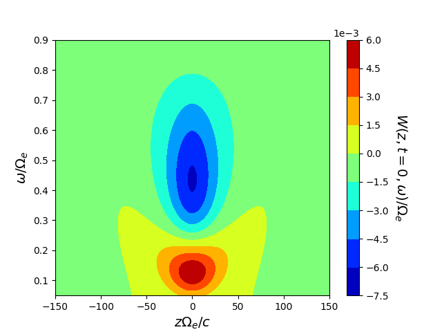
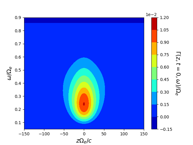
(a)                                                             (b)

Figure 1: Contour plots of $W(z,t=0,\omega)/\Omega_{e}$ (a) and $\Gamma(z,t=0,\omega)/\Omega_{e}$ (b) are shown for normalized parameters $\omega_{p}/\Omega_{e}=5$, $n_{e}/n=6\times 10^{-3}$, $w_{\parallel e}=0.2c$, $w_{\perp e}=0.53c$, $\xi=8.62\times 10^{-5}\Omega_{e}^{2}/c^{2}$.

2.3 Whistler wave packet propagation

As noted in Sec. 2.1, “due to the large separation between wavelength and magnetic field line scale length, we can describe whistler waves as wave packets propagating in a weakly nonuniform medium” [6, 31, 83]. In particular, by letting

$$\delta\bar{\bm{E}}_{\perp k}(z,t)=\hat{\bm{e}}|\delta\bar{\bm{E}}_{\perp k}(z,t)|e^{i\varphi_{k}(z,t)}\;,$$ (21)

with $\hat{\bm{e}}$ the polarization vector defined such $\hat{\bm{e}}\cdot\hat{\bm{z}}=0$ and $\hat{\bm{e}}\cdot\hat{\bm{e}}^{*}=1$; and introducing

$$I_{k}(z,t)\equiv\left|\partial D_{w}/\partial k\right||\delta\bar{\bm{E}}_{\perp k}(z,t)|^{2}\;,$$ (22)

the evolution equation for $I_{k}(z,t)$ is

$$\left(\frac{\partial}{\partial t}+v_{gk}\frac{\partial}{\partial z}\right)I_{k}(z,t)=2\gamma_{k}I_{k}(z,t)=2\Gamma(z,t,\omega)I_{k}(z,t)\;,$$ (23)

where $v_{gk}=-(\partial D_{w}/\partial\omega_{k})^{-1}\partial D_{w}/\partial k$ is the wave-packet group velocity and

$$\gamma_{k}=-\frac{D_{Ak}^{1}}{\partial D_{w}/\partial\omega_{k}}$$ (24)

represents the wave packet driving rate due to the supra-thermal electrons. In fact, noting $\partial_{z}\partial_{k}D_{w}=0$, which allows us to identify the adjoint of $D_{w}$ with its complex conjugate [34],

$$D_{Ak}^{1}=\mathbb{I}{\rm m}\left(\frac{4\pi i}{\omega_{k}}\frac{\delta\bar{\bm{J}}_{hk}\cdot\delta\bar{\bm{E}}_{\perp k}^{*}}{|\delta\bar{\bm{E}}_{\perp k}(z,t)|^{2}}\right)\;$$ (25)

is the anti-Hermitian part of the (perturbed) dielectric constant. Equation (23) is derived by taking the scalar product of Eq. (6) with $\delta\bar{\bm{E}}^{*}_{\perp k}(z,t)$ and then treating it as wave equation in a slowly-varying weakly non-uniform medium [6, 31]. Meanwhile, the phase shift $\varphi_{k}(z,t)$ is given by

$$\left(\frac{\partial}{\partial t}+v_{gk}\frac{\partial}{\partial z}\right)\varphi_{k}(z,t)=\frac{D_{Rk}^{1}}{\partial D_{w}/\partial\omega_{k}}=-W(z,t,\omega)\;,$$ (26)

where

$$D_{Rk}^{1}=\mathbb{R}{\rm e}\left(\frac{4\pi i}{\omega_{k}}\frac{\delta\bar{\bm{J}}_{hk}\cdot\delta\bar{\bm{E}}_{\perp k}^{*}}{|\delta\bar{\bm{E}}_{\perp k}(z,t)|^{2}}\right)\;,$$ (27)

is the Hermitian part of the (perturbed) dielectric constant. Thus, all relevant nonlinear physics is included in the wave-particle interactions between whistler waves and supra-thermal electrons. More precisely, it is all described by the two functions $W(z,t,\omega)$ and $\Gamma(z,t,\omega)$ introduced in Eq. (16), derived in Sec. 2.2 and then specialized to Eqs. (18) and (20) in the linear limit. We will see in Sec. 3 that Eq. (18) still holds in the nonlinear case.

In the light of the discussion above, Eqs. (23) and (26) describe both linear and nonlinear evolution of the whistler wave spectrum excited by supra-thermal electrons once $W(z,t,\omega)$ and $\Gamma(z,t,\omega)$ are given. These equations are solved by the method of characteristics, where, given the lowest order WKB dispersion relation, Eq. (8), all fields with a subscript $k=K(z,\omega)$ must be interpreted as functions in the $(z,\omega)$ space. That is, $I_{k}(z,t)|_{k=K(z,\omega)}\equiv I(z,t,\omega)$, $\varphi_{k}(z,t)|_{k=K(z,\omega)}\equiv\varphi(z,t,\omega)$ and the group velocity $v_{gk}(z)|_{k=K(z,\omega)}=v_{g}(z,\omega)$. Defining a wave packet time variable

$$T_{\omega}(z)\equiv\int_{0}^{z}\frac{dz^{\prime}}{v_{g}(z^{\prime},\omega)}\;,$$ (28)

and its inverse

$$T^{-1}_{\omega}T_{\omega}(z)\equiv z\;;$$ (29)

the initial position, $z_{0}$, at $t=0$ of a wave packet located at position $z$ at time $t$ is then given by $T_{\omega}(z)-T_{\omega}(z_{0})=t$; or, equivalently

$$z_{0}(z,t)=T^{-1}_{\omega}T_{\omega}(z_{0})=T_{\omega}^{-1}(T_{\omega}(z)-t)\;.$$ (30)

It is then straightforward to show that

$$\partial_{t}\left[T_{\omega}^{-1}(T_{\omega}(z)-t)\right] = -v_{g}\left(T_{\omega}^{-1}(T_{\omega}(z)-t),\omega\right)\;,$$

$$\partial_{z}\left[T_{\omega}^{-1}(T_{\omega}(z)-t)\right] = v_{g}\left(T_{\omega}^{-1}(T_{\omega}(z)-t),\omega\right)/v_{g}(z,\omega)\;.$$ (31)

Given Eq. (31), one may verify by direct substitution that

$$I(z,t,\omega)=I_{\omega 0}\left(T_{\omega}^{-1}(T_{\omega}(z)-t)\right)$$

$$\hskip 20.00003pt\times\exp\left(2\int_{T_{\omega}^{-1}(T_{\omega}(z)-t)}^{z}\frac{dz^{\prime}}{v_{g}(z^{\prime},\omega)}\Gamma(z^{\prime},t-T_{\omega}(z)+T_{\omega}(z^{\prime}),\omega)\right)\;,$$ (32)

and

$$\varphi(z,t,\omega)=\varphi_{\omega 0}\left(T_{\omega}^{-1}(T_{\omega}(z)-t)\right)$$

$$\hskip 20.00003pt-\int_{T_{\omega}^{-1}(T_{\omega}(z)-t)}^{z}\frac{dz^{\prime}}{v_{g}(z^{\prime},\omega)}W(z^{\prime},t-T_{\omega}(z)+T_{\omega}(z^{\prime}),\omega)\;,$$ (33)

are solutions of Eqs. (23) and (26). Here, $I_{\omega 0}(z)=I(z,0,\omega)$ and $\varphi_{\omega 0}(z)=\varphi(z,0,\omega)$ are the initial conditions for the considered wave packet. In fact, using Eq. (31), one can show that, assuming $I_{\omega 0}(z)=$ const for simplicity,

$$\frac{\partial_{t}I}{2I} = \Gamma\left(T_{\omega}^{-1}(T_{\omega}(z)-t),0,\omega\right)$$ (34)

$$+\int_{T_{\omega}^{-1}(T_{\omega}(z)-t)}^{z}\frac{dz^{\prime}}{v_{g}(z^{\prime},\omega)}\partial_{t}\Gamma(z^{\prime},t-T_{\omega}(z)+T_{\omega}(z^{\prime}),\omega)\;;$$

$$\frac{\partial_{z}I}{2I} = \frac{1}{v_{g}(z,\omega)}\left[\Gamma\left(z,t,\omega\right)-\Gamma\left(T_{\omega}^{-1}(T_{\omega}(z)-t),0,\omega\right)\right]$$ (35)

$$+\int_{T_{\omega}^{-1}(T_{\omega}(z)-t)}^{z}\frac{dz^{\prime}}{v_{g}(z^{\prime},\omega)}\partial_{z}\Gamma(z^{\prime},t-T_{\omega}(z)+T_{\omega}(z^{\prime}),\omega)\;.$$

Analogous equations can be written for $\partial_{t}\varphi$ and $\partial_{z}\varphi$. Again, Eqs. (32) and (33) completely describe the linear and nonlinear evolution of the system, once $W(z,t,\omega)$ and $\Gamma(z,t,\omega)$ are given. Noting that $\partial_{t}\Gamma\left(z,t,\omega\right)=0$ in the linear limit, Eq. (34), in particular, has two major implications: (i) the whistler instability is of convective type (it does not grow exponentially at the same rate everywhere in the time asymptotic limit); (ii) chorus chirping is a nonlinear process. In fact, assuming that chirping occurs, the behavior of $I(z,t,\omega)$ at a given frequency and position should first increase in time and then decrease, reaching a maximum during the time interval corresponding to the chorus element crossing the considered frequency at the given position. In order for this to be possible in the linear limit; i.e., for $\partial_{t}\Gamma\left(z,t,\omega\right)=0$, we should have $\Gamma\left(T_{\omega}^{-1}(T_{\omega}(z)-t),0,\omega\right)=0$ at the considered frequency and given position, which clearly cannot be the case.

In order to illustrate the linear spatiotemporal structures of the whistler wave packets excited by supra-thermal electrons, Fig. 2 shows contour plots in the $(\omega,t)$ plane of $I(z,t,\omega)/I_{\omega 0}$ and $\varphi(z,t,\omega)$ assuming $I_{\omega 0}={\rm const.}$ and $\varphi_{\omega 0}=0$. For simplicity, only wave packets with positive $k$ and correspondingly positive group velocity are considered, with $W(z,0,\omega)$ and $\Gamma(z,0,\omega)$ given by Eq. (20). Top panels (a) and (b) in Fig. 2 refer to $z=0$; i.e.  to the fluctuation intensity and phase at the equator, where the supra-thermal electron source is strongest. Meanwhile, panels (c) and (d) are, respectively, the analogue of panels (a) and (b) at $z=50c/\omega_{e}$, where the hot electron source has significantly decayed but the wave packet has traveled though the whole source region.

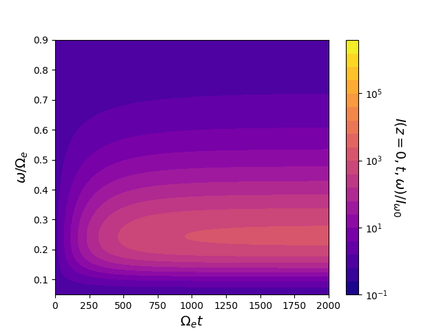
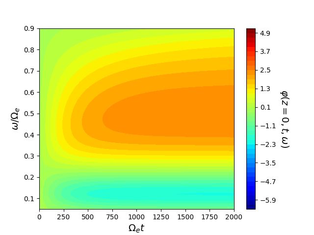
(a)                                                             (b)

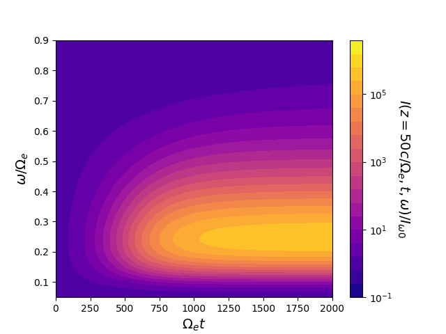
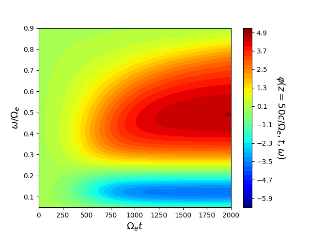
(c)                                                             (d)

Figure 2: Contour plots in the $(\omega,t)$ plane that illustrate the linearized time evolution of $I(z,t,\omega)/I_{\omega 0}$ and $\varphi(z,t,\omega)$ assuming $I_{\omega 0}={\rm const.}$ and $\varphi_{\omega 0}=0$. Physical parameters are those of Fig. 1. Top panels (a) and (b) refer to $z=0$; while panels (c) and (d) are their analogue at $z=50c/\omega_{e}$.

Finally, for $\omega=\omega_{0}\simeq 0.241\Omega_{e}$, corresponding to the strongest growing frequency at the equator in Fig. 1, Fig. 3 shows snapshots of the spatial structure of both $I(z,t,\omega_{0})/I_{\omega 0}$ (a) and $\varphi(z,t,\omega_{0})$ (b) assuming $I_{\omega 0}={\rm const.}$ and $\varphi_{\omega 0}=0$.

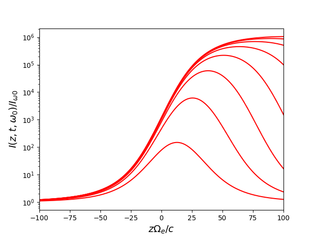
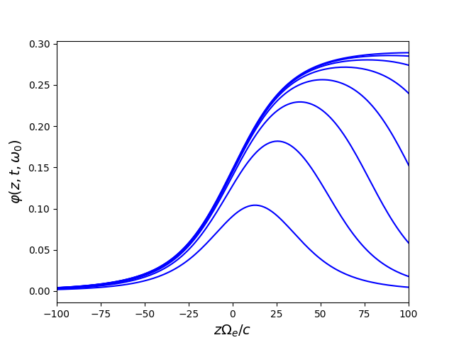
(a)                                                             (b)

Figure 3: Snapshots at times $\Omega_{e}t=250,500,...,2000$ that illustrate the linearized time evolution of $I(z,t,\omega_{0})/I_{\omega 0}$ (a) and $\varphi(z,t,\omega_{0})$ (b) assuming $I_{\omega 0}={\rm const.}$ and $\varphi_{\omega 0}=0$. Increasingly higher-valued curves correspond to later times. Physical parameters are those of Fig. 1.

After the initial peaking of both $I(z,t,\omega_{0})$ and $\varphi(z,t,\omega_{0})$ at $z\simeq 0$, where the growth rate is strongest, the propagation of the whistler wave packet at the group velocity along the magnetic field line becomes increasingly more evident. For sufficiently large $z$, such that it is outside the “hot electron” source region (cf. Sec. 4.1), Eqs. (32) and (33) suggest that spatiotemporal dependences can be only on $T_{\omega}^{-1}(T_{\omega}(z)-t)$. Time asymptotically, when wave packets have traveled all the way from $z\rightarrow-\infty$ to $z\rightarrow\infty$, $I(z,t,\omega_{0})$ and $\varphi(z,t,\omega_{0})$ reach a constant shape, which depends on $\omega_{0}$ only.

3 Phase space transport and nonlinear dynamics

In this section, we introduce the nonlinear dynamics starting from the basic kinematic description of single particle motion and wave particle trapping in Sec. 3.1. A phase space hole is created during this process near resonance: that is, a phase space density difference between the center of the resonant structure and the “unperturbed surrounding”. The phase space structure is called “phase space hole/clump” depending on the sign of Eq. (46). The dynamic description of phase space nonlinear behaviors is given in Sec. 3.2, where we focus on the nonlinear particle response without fast temporal or spatial dependences, which correspond to the self-interaction of the wavenumber of interest with itself. This nonlinear response obeys to the evolution equation, Eq. (55), which may look like a “quasilinear” description at first glance but is, indeed, much more general as will be shown and discussed in the following. For the more theoretically inclined readers, we will delineate the close connection of the present approach with the Dyson equation and the so-called “principal series” of secular terms. Conservation properties of the adopted reduced description are discussed in Sec. 3.3, where we also analyze the different nonlinear dynamic behaviors that are possibly described within the present theoretical framework, anticipating some of the qualitative features of chorus excitation, which are addressed in Sec. 4.

3.1 Single particle motion and wave particle trapping

The equations of motion of single particles (electrons) interacting with the whistler wave packet described in Sec. 2 are the natural starting point for analyzing nonlinear dynamics. Noting Eq. (11) to extract the components of the Lorentz force, it is possible to write

$$\dot{v}_{\perp}=\frac{v_{\|}v_{\perp}}{2\Omega}\frac{d\Omega}{dz}-\frac{e}{m}\left(\frac{kv_{\|}}{\omega}-1\right)\delta\bar{E}_{k}\sin\phi\;,$$

$$\dot{v}_{\|}=-\frac{v_{\perp}^{2}}{2\Omega}\frac{d\Omega}{dz}+\frac{e}{m}\frac{kv_{\perp}}{\omega}\delta\bar{E}_{k}\sin\phi\;,$$

$$\dot{\phi}=\Omega-\omega+kv_{\|}-\frac{e}{mv_{\perp}}\left(\frac{kv_{\|}}{\omega}-1\right)\delta\bar{E}_{k}\cos\phi\;,$$ (36)

where $\phi\equiv\alpha+S_{k}$, and we recalled that $\dot{\alpha}=\Omega$ (the positive definite electron cyclotron frequency) and $\delta\bar{E}_{k}\equiv\left(\delta\bar{\bm{E}}_{\perp k}\right)_{x}$ for brevity, which is assumed as real without loss of generality. Noting that the considered wave packet is right handed circularly polarized, and $\left(\delta\bar{\bm{B}}_{\perp k}\right)_{y}=(kc/\omega)\left(\delta\bar{\bm{E}}_{\perp k}\right)_{x}$, Eqs. (36) are readily cast in the standard form adopted by [17, 40, 26, 71, 44, 53, 2] and, more recently, in the brief review by [60]. In terms of the magnetic moment, $\mu=v_{\perp}^{2}/2$, and the energy per unit mass, ${\cal E}=v^{2}/2$, Eqs. (36) can be rewritten as

$$\dot{\mu}=-\frac{e}{m}\left(\frac{kv_{\|}}{\omega}-1\right)\left(\frac{2\mu}{B}\right)^{1/2}\delta\bar{E}_{k}\sin\phi\;,$$

$$\dot{\cal E}=\frac{e}{m}\left(2\mu B\right)^{1/2}\delta\bar{E}_{k}\sin\phi\;,$$

$$\dot{\phi}=\Omega-\omega+kv_{\|}\;,$$ (37)

where, in the latter equation, we have dropped the negligible contribution to $\dot{\phi}$ due $\propto\delta\bar{E}_{k}$ (cf., e.g., any of the above references in this subsection). The resonance velocity is given by $\dot{\phi}=0$ and, thus,

$$v_{r}=\frac{\omega-\Omega}{k}\;.$$ (38)

Equations (9) and (38) show that the resonant velocity of the considered whistler wave packet has opposite sign with respect to the corresponding phase and group velocities. Noting that $\dot{\phi}=k(v_{\parallel}-v_{r})$, it is readily shown that, near resonance,

$$\ddot{\phi}=k\frac{d}{dt}(v_{\parallel}-v_{r})\;,$$ (39)

where the total time derivative along the moving wave packet is expressed as

$$\frac{d}{dt}=\frac{\partial}{\partial t}+v_{g}\frac{\partial}{\partial z}\;.$$ (40)

Using Eqs. (9) and (38) along with the equations of motion, Eqs. (36), and assuming constant $\omega_{p}^{2}$ along the magnetic field line, one can show, after some lengthy but straightforward algebra (cf., e.g., [72, 44]),

$$\ddot{\phi}=\omega_{\rm tr}^{2}\left(\sin\phi-R\right)\;,$$ (41)

where [72, 44]

$$R=\frac{1}{\omega_{\rm tr}^{2}}\left[\left(1-\frac{v_{r}}{v_{g}}\right)^{2}\frac{\partial\omega}{\partial t}+\left(\frac{kv_{\perp}^{2}}{2\Omega}-\frac{3}{2}v_{r}\right)\frac{\partial\Omega}{\partial z}\right]\;,$$ (42)

and $\omega_{\rm tr}^{2}=kv_{\perp}(e/m)k\delta\bar{E}_{k}/\omega=kv_{\perp}(e\delta\bar{B}_{ky}/mc)$. The derivation of $R$ expression is based on kinematics and wave dispersive properties only; and follows from direct calculation of $kdv_{r}/dt$ [72, 44]. For $R=0$, Eq. (41) is a nonlinear pendulum equation with $\omega_{\rm tr}$ giving the frequency of small amplitude oscillations. For $|R|<1$, structures are formed in the $(\phi,\dot{\phi})$ phase space due to wave particle trapping. This is shown in Fig. 4 for $R=1/2$. Meanwhile, no structure formation is possible for $|R|>1$, as can be seen integrating once Eq. (41), yielding

$$(1/2)\dot{\phi}^{2}+\omega_{\rm tr}^{2}\left(\cos\phi+R\phi\right)={\rm const}\;.$$ (43)

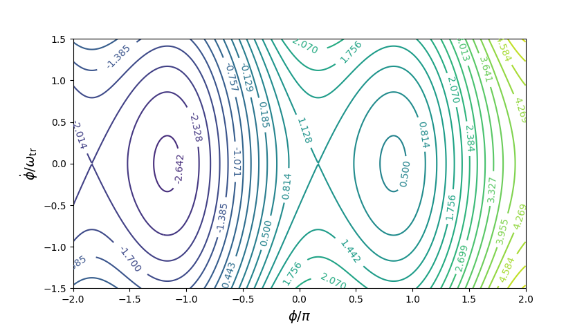
Figure 4: Contour plot of Eq. (43) in the $(\phi,\dot{\phi})$ phase space showing structure formation due to wave particle trapping for $R=1/2$.

We will come back to the importance of this condition in Sec. 4, since $R$ is evidently connected with the frequency chirping of the whistler wave packet from its definition, Eq. (42). Here, we further note that, unlike the usual nonlinear pendulum case, the separatrix identifying phase space oscillations for $|R|<1$ has one single X-point. Again, we will discuss the important implications of this fact in Sec. 4.

Near resonance, Eqs. (37) imply that

$$\dot{\mu}B\omega=\Omega\dot{\cal E}\;,\;\;\;\;\;\Rightarrow\;\;\;\;\;\omega d\mu=(\Omega/B)d{\cal E}\;.$$ (44)

Thus, the increase/decrease of perpendicular energy due to wave-particle interaction is larger than the corresponding increase/decrease of total energy for $0<\omega<\Omega$. Said differently, an increase in magnetic moment and energy of a resonant particle is necessarily accompanied by a decrease in the parallel energy and vice versa. Considering, e.g., a rising tone chorus element (cf. Sec. 4 for details) and, for simplicity, only wave packets with positive $k$ as we did in Sec. 2, resonant velocity, Eq. (38), is negative and becomes progressively less negative (resonant velocity increases). Thus, a phase locked resonant particle, such as those that are deeply trapped near O-points of structures in the $(\phi,\dot{\phi})$ phase space in Fig. 4, looses parallel energy in the chirping process and, at the same time, gains total energy as well as magnetic moment. It can be shown that a phase space hole is created during this process near resonance. In fact, by rewriting Eq. (17) as

$$f_{0}=\frac{n_{e}}{(2\pi)^{3/2}w_{\|e}w_{\perp e}^{2}}\exp\left(-\mathcal{E}/w_{\|e}^{2}+A\mu B_{e}/w_{\perp e}^{2}\right)\;,$$ (45)

we can evaluate the phase space density difference, $\Delta f_{0}$, between the center of the resonant structure and the “unperturbed surrounding”. The center of the resonant structure is characterized by $f_{0}$ at the original $\mathcal{E}$ and $\mu$. Meanwhile the unperturbed surrounding is characterized by $f_{0}$ at the $\mathcal{E}+\Delta\mathcal{E}$ and $\mu+\Delta\mu$. Thus, using Eq. (44) and recalling $A=w_{\perp e}^{2}/w_{\parallel e}^{2}-1$ [40, 72, 44, 60]

$$\Delta f_{0} = f_{0}({\cal E},\mu)-f_{0}({\cal E}+\Delta{\cal E},\mu+\Delta\mu)\;,$$ (46)

$$\propto \frac{\Delta\mathcal{E}}{w_{\|e}^{2}}-AB_{e}\frac{\Delta\mu}{w_{\perp e}^{2}}=-AB_{e}\frac{\Delta\mu}{w_{\parallel e}^{2}}\left(\frac{A}{A+1}-\frac{\omega}{\Omega_{e}}\right)\;.$$

Depending on the negative/positive sign of Eq. (46), the resonant phase space structure is called “phase space hole/clump”. This demonstrates that phase space hole is formed near resonance for a rising tone chorus element characterized by $\Delta\mu>0$ [cf. discussion between Eqs. (44) and (45)], which tends to disappear when the whistler wave instability is lost for $\omega/\Omega_{e}=A/(A+1)$, consistent with Eq. (20) and Fig. 1(b). The same argument can be used to show that a phase space clump occurs near resonance for a falling tone chorus element.

3.2 Small amplitude expansion and renormalized electron response

Addressing nonlinear dynamics and phase space transport underlying the evolution of whistler wave packet excited by supra-thermal electrons requires analyzing the self-consistent energetic electron response in the presence of a small but finite fluctuation level. In Sec. 2, we have noted that the effect of supra-thermal electrons can be treated as a perturbation, with wave dispersive properties remaining those of a right-hand circular polarized whistler wave propagating parallel to the Earth’s magnetic field. The convective amplification of the whistler wave packet by the energetic electron source, localized nearby the equator, suggests that the fluctuation level remains small (e.g., $|\delta\bar{\bm{B}}_{\perp k}/B|\ll 1$) during the nonlinear evolution and, thus, that the self-consistent electron response may be computed assuming a small amplitude expansion. That is, we assume that the electron distribution function can be formally written as an asymptotic series

$$f=f^{(0)}+f^{(1)}+f^{(2)}+\ldots\;,$$ (47)

where the superscripts $(n)$ denote the power at which fluctuation amplitude enters in each term. The first two terms are those that we analyzed in Sec. 2. More precisely, noting Eq. (12), $f^{(0)}=f_{0}(\bm{v},z)$ is the reference equilibrium distribution function, while $f^{(1)}$ corresponds to terms $\propto\delta\bar{f}_{k}(\bm{v},z,t)$ and c.c. Noting the form of the nonlinear Vlasov equation

$$\left(\frac{\partial}{\partial t}+v_{\parallel}\frac{\partial}{\partial z}+\Omega\frac{\partial}{\partial\alpha}\right)f-\frac{e}{m}\left(\delta\bm{E}_{\perp}+\frac{\bm{v}\times\delta\bm{B}_{\perp}}{c}\right)\cdot\frac{\partial}{\partial\bm{v}}f=0\;;$$ (48)

and the structure of the nonlinear coupling term that can still be represented by Eq. (11), it can be shown that the natural extension of equation Eq. (12) is

$$f^{(2)} = \frac{1}{2}\sum_{k,k^{\prime}}\left(e^{iS_{k}(z,t)+iS_{k^{\prime}}(z,t)+2i\alpha}\delta\bar{f}_{k+k^{\prime}}(\bm{v},z,t)+c.c.\right)$$ (49)

$$+\frac{1}{2}\sum_{k,k^{\prime}}\left(e^{iS_{k}(z,t)-iS_{k^{\prime}}(z,t)}\delta\bar{f}_{k-k^{\prime}}(\bm{v},z,t)+c.c.\right)\;.$$

By direct substitution of Eq. (49) into Eq. (48), we obtain

$$\left[2\Omega+(k+k^{\prime})v_{\parallel}-(\omega_{k}+\omega_{k^{\prime}})-i(\partial_{t}+v_{\parallel}\partial_{z})\right]\delta\bar{f}_{k+k^{\prime}}=\frac{e}{m}\frac{v_{\perp}}{4}\left\{\delta\bar{E}_{k}\left[\bar{\partial}_{{\cal E}k}\right.\right.$$

$$\hskip 10.00002pt\left.\left.-\frac{1}{v_{\perp}^{2}}\left(1-\frac{kv_{\|}}{\omega_{k}}\right)\right]\delta\bar{f}_{k^{\prime}}+\delta\bar{E}_{k^{\prime}}\left[\bar{\partial}_{{\cal E}{k^{\prime}}}-\frac{1}{v_{\perp}^{2}}\left(1-\frac{k^{\prime}v_{\|}}{\omega_{k^{\prime}}}\right)\right]\delta\bar{f}_{k}\right\},$$ (50)

where we introduced the abbreviated notation

$$\bar{\partial}_{{\cal E}k} \equiv \left[\frac{k}{\omega_{k}}\frac{\partial}{\partial v_{\|}}+\left(1-\frac{kv_{\|}}{\omega_{k}}\right)\frac{1}{v_{\perp}}\frac{\partial}{\partial v_{\perp}}\right]$$ (51)

$$= \left[\frac{\partial}{\partial{\cal E}}+\left(1-\frac{kv_{\|}}{\omega_{k}}\right)\frac{1}{B}\frac{\partial}{\partial\mu}\right]\;;$$

and

$$\left[(k-k^{\prime})v_{\parallel}-(\omega_{k}-\omega_{k^{\prime}})-i(\partial_{t}+v_{\parallel}\partial_{z})\right]\delta\bar{f}_{k-k^{\prime}}=\frac{e}{m}\frac{v_{\perp}}{4}\left\{\delta\bar{E}_{k}\left[\bar{\partial}_{{\cal E}k}+\frac{1}{v_{\perp}^{2}}\right.\right.$$

$$\hskip 10.00002pt\times\left.\left.\left(1-\frac{kv_{\|}}{\omega_{k}}\right)\right]\delta\bar{f}_{k^{\prime}}^{*}-\delta\bar{E}_{k^{\prime}}^{*}\left[\bar{\partial}_{{\cal E}{k^{\prime}}}+\frac{1}{v_{\perp}^{2}}\left(1-\frac{k^{\prime}v_{\|}}{\omega_{k^{\prime}}}\right)\right]\delta\bar{f}_{k}\right\}\;.$$ (52)

Note the normalizations on the right hand side of Eqs. (50) and (52) to avoid double counting for $k\leftrightarrow k^{\prime}$; and that, on the left hand side, the operators $(\partial_{t}+v_{\parallel}\partial_{z})$ account for the residual slow spatiotemporal dependences consistent with the considered wave packet representation. A particular important role is played by the $k=k^{\prime}$ response in Eq. (52). It is readily noted that this contribution is not characterized by any fast temporal nor spatial dependences. Thus, by all means, $\delta\bar{f}_{0}$ (and its c.c.) should be considered as a modification of the considered original equilibrium due to self interactions of the fluctuation spectrum; i.e., $f_{0}$ of Eq. (17) and/or Eq. (45), should be replaced by

$$f_{0}\rightarrow f_{0}+\sum_{k}\mathbb{R}{\rm e}\delta\bar{f}_{0}\;,$$ (53)

with $\delta\bar{f}_{0}$ solution of Eq. (52) for $k^{\prime}=k$ [83]:

$$(\partial_{t}+v_{\parallel}\partial_{z})\delta\bar{f}_{0}=\frac{e}{m}\frac{v_{\perp}}{4}\sum_{k}i\left\{\delta\bar{E}_{k}\left[\bar{\partial}_{{\cal E}k}+\frac{1}{v_{\perp}^{2}}\right.\right.$$

$$\hskip 10.00002pt\times\left.\left.\left(1-\frac{kv_{\|}}{\omega_{k}}\right)\right]\delta\bar{f}_{k}^{*}-\delta\bar{E}_{k}^{*}\left[\bar{\partial}_{{\cal E}{k}}+\frac{1}{v_{\perp}^{2}}\left(1-\frac{kv_{\|}}{\omega_{k}}\right)\right]\delta\bar{f}_{k}\right\}\;.$$ (54)

If we schematically illustrate Eq. (13) borrowing the Feynman diagram in Fig. 5(a), [79, 78, 11, 83], the modification of the original equilibrium defined in Eq. (53) corresponds to the simple loop diagram in Fig. 5(b); that is, to the emission and reabsorption of the same-$k$ fluctuations, interpreted as quanta, summed-up over the whole spectrum.

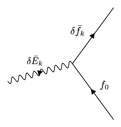
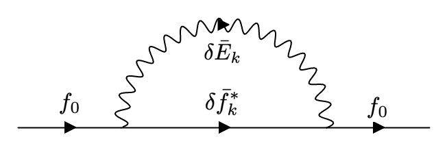
(a)                                                             (b)

Figure 5: Schematic illustration of Eq. (13) borrowing Feynman diagrams with suitably adapted rules (a) [79, 78, 11, 83]; and modification of the original equilibrium defined in Eq. (53) represented as simple loop diagram (b).

Quite interesting, the solution of Eq. (53), $\delta\bar{f}_{0}$, grows secularly in time as $\sim t$ on a sufficiently short time scale. Even further, by iterating the procedure and substituting the “updated” $f_{0}$, according to Eq. (53), into the expression for $\delta\bar{f}_{k}$, Eq. (13), we could calculate a correspondingly “updated” expression $\delta\bar{f}_{0}$ from Eq. (54), whose secularities would grow as $\sim t^{2}$, and so on. This behavior is well known in the general procedure used for deriving kinetic equations in weakly non-ideal systems [70, 47, 5], and is what dominates the so-called “principal series” of secular terms obtained by formal perturbation expansion in powers of fluctuating fields. If fluctuations of the spectrum are replaced by unstable oscillations, it can be shown that the $\sim t^{\ell}$ secularities are replaced by terms $\sim(\omega_{k}/\gamma_{k})^{\ell}$ [37, 3], with $\gamma_{k}$ the growth rate of the $\omega_{k}$ fluctuation. The essence, however, remains unchanged, and the “principal series” still dominates the $f_{0}$ response. In fact, other terms in the perturbation expansion, at each order, would be at least $\sim 1/(\omega_{k}\tau_{NL})\sim(\gamma_{k}/\omega_{k})$ smaller, with $\tau_{NL}$ the characteristic nonlinear time. As a matter of fact, the overall response of the “principal series” is obtained from the solution of

$$(\partial_{t}+v_{\parallel}\partial_{z})f_{0}=\frac{e}{m}\frac{v_{\perp}}{4}\mathbb{R}{\rm e}\sum_{k}i\left\{\delta\bar{E}_{k}\left[\bar{\partial}_{{\cal E}k}+\frac{1}{v_{\perp}^{2}}\right.\right.$$

$$\hskip 10.00002pt\times\left.\left.\left(1-\frac{kv_{\|}}{\omega_{k}}\right)\right]\delta\bar{f}_{k}^{*}-\delta\bar{E}_{k}^{*}\left[\bar{\partial}_{{\cal E}{k}}+\frac{1}{v_{\perp}^{2}}\left(1-\frac{kv_{\|}}{\omega_{k}}\right)\right]\delta\bar{f}_{k}\right\}\;,$$ (55)

with Eq. (17) as initial condition. In fact, it can be verified that the iterative solution of Eqs. (13) and (55) generates the whole Dyson series represented by all loop diagrams in Fig. 6.

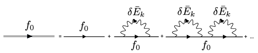
Figure 6: Schematic illustration of the Dyson series iterative solution of Eqs. (13) and (55).

Thus, we dub Eq. (55) as Dyson-like equation [16, 51, 27], noting that it gives the renormalized electron response as evolution of the considered original equilibrium due to self interactions of the fluctuation spectrum [79, 78, 11, 83].

The Dyson-like equation, Eq. (55), can be considered as an asymptotic representation of the renormalized electron response, where the asymptotic expansion parameter is $\sim 1/(\omega_{k}\tau_{NL})\sim(\gamma_{k}/\omega_{k})\ll 1$. Meanwhile, nonlinear interactions in Eqs. (50) and (52) generally modify the evolution equation for $\delta\bar{f}_{k}$. Similar to the argument leading us to Eq. (55), dominant nonlinear interactions are those corresponding to emission and reabsorption of the same quanta [70, 47, 5, 3, 15, 1, 74, 36]. It can be verified by inspection that these “diagonal interactions”, which renormalize the evolution operator for $\delta\bar{f}_{k}$, are obtained by two contributions: (i) coupling the $\delta\bar{f}_{k+k^{\prime}}$ in Eq. (50) with the complex conjugate of $k^{\prime}$ expression in Eq. (11); (ii) coupling the $\delta\bar{f}_{k-k^{\prime}}$ in Eq. (52) and its complex conjugate by exchanging $k\leftrightarrow k^{\prime}$ with the $k^{\prime}$ expression in Eq. (11). The former contribution produces

$$-i\Delta_{1k} \equiv i\frac{e^{2}}{m^{2}}\frac{v_{\perp}^{2}}{8}\sum_{k^{\prime}}\delta\bar{E}_{k^{\prime}}^{*}\left[\bar{\partial}_{{\cal E}k^{\prime}}+\frac{2}{v_{\perp}^{2}}\left(1-\frac{k^{\prime}v_{\parallel}}{\omega_{k^{\prime}}}\right)\right]$$ (56)

$$\times{\cal P}_{k+k^{\prime}}\delta\bar{E}_{k^{\prime}}\left[\bar{\partial}_{{\cal E}k^{\prime}}-\frac{1}{v_{\perp}^{2}}\left(1-\frac{k^{\prime}v_{\parallel}}{\omega_{k^{\prime}}}\right)\right]\;,$$

to be added on the left hand side in the evolution equation for $\delta\bar{f}_{k}$. Here, we have introduced the ${\cal P}_{k+k^{\prime}}$ propagator:

$${\cal P}_{k+k^{\prime}}\equiv\left[2\Omega+(k+k^{\prime})v_{\parallel}-(\omega_{k}+\omega_{k^{\prime}})-i(\partial_{t}+v_{\parallel}\partial_{z})\right]^{-1}\;,$$ (57)

defined as the inverse of the operator in the square parentheses. Meanwhile, the second contribution produces an analogous term

$$-i\Delta_{2k} \equiv i\frac{e^{2}}{m^{2}}\frac{v_{\perp}^{2}}{8}\sum_{k^{\prime}\neq k}\delta\bar{E}_{k^{\prime}}\bar{\partial}_{{\cal E}k^{\prime}}{\cal P}_{k-k^{\prime}}\delta\bar{E}_{k^{\prime}}^{*}\left[\bar{\partial}_{{\cal E}k^{\prime}}+\frac{1}{v_{\perp}^{2}}\left(1-\frac{k^{\prime}v_{\parallel}}{\omega_{k^{\prime}}}\right)\right]\;,$$ (58)

with

$${\cal P}_{k-k^{\prime}}\equiv\left[(k-k^{\prime})v_{\parallel}-(\omega_{k}-\omega_{k^{\prime}})-i(\partial_{t}+v_{\parallel}\partial_{z})\right]^{-1}\;.$$ (59)

Thus, taking diagonal interactions into account, Eq. (13) is replaced by

$$\delta\bar{f}_{k} = \frac{e}{m}{\cal P}_{k}v_{\perp}\delta\bar{E}_{k}\bar{\partial}_{{\cal E}k}f_{0}\;,$$ (60)

$${\cal P}_{k} \equiv \left[\Omega+kv_{\parallel}-\omega_{k}-i(\partial_{t}+v_{\parallel}\partial_{z})-\Delta_{k}\right]^{-1}\;;$$ (61)

with $\Delta_{k}\equiv\Delta_{1k}+\Delta_{2k}$ describing both nonlinear resonance frequency shift as well as resonance broadening [15, 1, 74, 36]. In the linear limit, Eq. (60) readily recovers Eq. (13). Meanwhile, allowing for leading order nonlinear interactions, Eqs. (55) and (60) fully describe the renormalized energetic electron response, self-consistently evolving with the fluctuation spectrum, described by Eqs. (23) and (26). In our applications to chorus chirping in Sec. 4, resonance broadening will be dropped in Eq. (61), since its effect is typically small in the parameter range where chorus is usually observed (cf. Sec. 3.3). As anticipated in Sec. 2, Eq. (18) for the wave particle power exchange remains valid nonlinearly, provided the renormalized expression of the propagator is used as in Eq. (61), instead of the linearized (algebraic) expression, $\left[\Omega+kv_{\parallel}-\omega_{k}\right]^{-1}$.

3.3 Conservation properties and phase space transport

Let’s reconsider the Dyson-like equation, Eq. (55), and rewrite it as

$$(\partial_{t}+v_{\parallel}\partial_{z})f_{0}+\frac{1}{v_{\perp}}\frac{\partial}{\partial v_{\perp}}\left(v_{\perp}S_{\perp}\right)+\frac{\partial}{\partial v_{\parallel}}S_{\parallel}=0\;.$$ (62)

Here, we have introduced

$$S_{\perp} \equiv \sum_{k}\frac{i}{4}\left(1-\frac{kv_{\parallel}}{\omega_{k}}\right)\delta\bar{E}_{k}^{*}\delta\bar{f}_{k}+c.c.\;,$$ (63)

$$S_{\parallel} \equiv \sum_{k}\frac{i}{4}\frac{kv_{\perp}}{\omega_{k}}\delta\bar{E}_{k}^{*}\delta\bar{f}_{k}+c.c.\;.$$ (64)

Integrating Eq. (62) in velocity space, $\left\langle...\right\rangle=2\pi\iint v_{\perp}dv_{\perp}dv_{\parallel}(...)$ with the notation introduced in Sec. 2, we have the continuity equation

$$\partial_{t}n+\partial_{z}(nu)=0\;,$$ (65)

where $nu$ is the parallel electron flux. Thus, particles are conserved. Similarly, taking the product of Eq. (62) times $mv_{\parallel}$ and performing the same integration, we have

$$\partial_{t}(mnu)+\partial_{z}\left\langle mv_{\parallel}^{2}f_{0}\right\rangle=\left\langle mS_{\parallel}\right\rangle\;.$$ (66)

Equation (66), expresses parallel momentum conservation accounting for wave-particle momentum exchange. Finally, multiplying Eq. (62) by $m{\cal E}$ and integrating in velocity space, denoting particle kinetic energy density by ${\cal K}=\left\langle m{\cal E}f_{0}\right\rangle$, we have

$$\partial_{t}{\cal K}+\partial_{z}\left\langle mv_{\parallel}{\cal E}f_{0}\right\rangle = \left\langle m\left(v_{\perp}S_{\perp}+v_{\parallel}S_{\parallel}\right)\right\rangle=-\sum_{k}\mathbb{I}{\rm m}\left\langle e\frac{v_{\perp}}{2}\delta\bar{E}_{k}^{*}\delta\bar{f}_{k}\right\rangle$$ (67)

$$= -\sum_{\omega}\Gamma(z,t,\omega)\omega\frac{\partial D_{w}}{\partial\omega}\left.\frac{|\delta\bar{\bm{E}}_{\perp k}|^{2}}{8\pi}\right|_{k=K(z,\omega)}$$

$$= -\left[\partial_{t}\sum_{k}W_{wk}+\partial_{z}\sum_{k}(v_{gk}W_{wk})\right]\;.$$

Here, in the second line we have used Eq. (16) and, in the third line, we have rewritten Eq. (23) introducing the wave energy density in the $k$ fluctuation as $W_{wk}\equiv\omega_{k}\partial_{\omega_{k}}D_{w}|\delta\bar{\bm{E}}_{\perp k}|^{2}/(16\pi)$ [6]. Thus, Eq. (67) expresses energy conservation. In conclusion, the Dyson-like equation, Eq. (55), properly describes phase space transport with all the necessary conservation properties.

A variety of different nonlinear dynamics behaviors are described by the self-consistent equations for fluctuation spectrum, Eqs. (23) and (26), and supra-thermal electron response, Eqs. (55) and (60). Starting from very low fluctuation level, e.g., with whistler waves excited by wave particle interactions out of thermal noise, the spectrum is generally very broad, with width $\Delta\omega\sim\omega$, as noted in Sec. 2. The resonance broadening effect is typically small, $\sim\omega_{{\rm tr}k}^{4}/(\gamma_{k}\Delta\omega^{3})$ and can be neglected. Meanwhile, the dense whistler wave spectrum causes particles to undergo quasilinear-type diffusion, consistently described by Eq. (55), which reduces to the quasilinear diffusion equation in this limit [20, 3]. The diffusion time is $\tau_{\rm diff}\sim\Delta\omega^{3}/\omega_{{\rm tr}k}^{4}\gg 1/\Delta\omega$, consistent with having small Kubo number, $K\sim\omega_{{\rm tr}k}/\Delta\omega\ll 1$. Since $\gamma_{k}\tau_{\rm diff}\sim\gamma_{k}\Delta\omega^{3}/\omega_{{\rm tr}k}^{4}\gg 1$, the wave can be significantly amplified before any significant diffusion has occurred. However, due to the convective nature of the whistler instability, saturation of fluctuation growth can be reached because the wave packet moves out of the source region and before nonlinear behavior becomes noticeable. Thus, we expect that there is a threshold in driving strength, due to a combination of initial level of whistler waves and convective amplification by linear instability, which determines the observed nonlinear behavior (cf. Sec. 4). Optimal ordering for the fluctuation amplitude needed to observe nonlinear oscillations would be obtained for

$$\tau_{NL}^{-1}\sim\gamma_{k}\sim\omega_{{\rm tr}k}\;.$$ (68)

When this condition is met, the mode does not stop growing by the well-known wave particle trapping mechanism discussed by [45, 46] for the beam-plasma instability, since phase mixing is slowed down by the presence of a broad spectrum (cf. discussion above). Estimating ${\cal P}_{k}\sim\tau_{NL}$ in Eq. (61), and $\bar{\partial}_{{\cal E}k}\sim(k^{2}/\omega_{k})/(k\Delta v)$, with $k\Delta v$ the resonance width, Eq. (55) suggests that nonlinear whistler wave packet dynamics be characterized by

$$\tau_{NL}^{-1}\sim\frac{\omega_{{\rm tr}k}^{2}}{k\Delta v}\raisebox{-3.01385pt}{$\stackrel{{\scriptstyle\textstyle>}}{{\sim}}$}\ k\Delta v\;;\;\;\;\;\;\Leftrightarrow\;\;\;\;\;\tau_{NL}^{-1}\raisebox{-3.01385pt}{$\stackrel{{\scriptstyle\textstyle>}}{{\sim}}$}\ \omega_{{\rm tr}k}\raisebox{-3.01385pt}{$\stackrel{{\scriptstyle\textstyle>}}{{\sim}}$}\ k\Delta v\;.$$ (69)

Note that this condition implies the Kubo number be of $\sim{\cal O}(1)$ and the corresponding nonlinear behavior described by Eq. (55) be non-perturbative. This is the reason why the Dyson-like equation must be solved as is and not by iterative perturbation expansion, since the Dyson series terms would have the Kubo number as expansion parameter. In this regime, that is typical of chorus excitation (cf. Sec. 4), resonance broadening is still negligible provided that the system is not too strongly driven. In fact, estimating ${\cal P}_{k\pm k^{\prime}}\sim\Delta\omega^{-1}$ in Eqs. (57) and (59), Eqs. (56) and (58) yield

$$\Delta_{k}\sim\frac{1}{\tau_{NL}\Delta\omega}\frac{1}{\tau_{NL}}<\frac{1}{\tau_{NL}}\;.$$ (70)

For the quasi-coherent chorus spectrum $\Delta\omega/\omega_{{\rm tr}k}\raisebox{-3.01385pt}{$\stackrel{{\scriptstyle\textstyle>}}{{\sim}}$}\ \tau_{NL}\Delta\omega>1$, and Eq. (70) is verified. Increasing the driving strength makes $\Delta\omega$ smaller. Eventually, when $\tau_{NL}\Delta\omega\sim 1$, a strong effect is expected from resonance broadening (cf., e.g., [32, 33]) and the coherent nature of chorus excitation will be lost. Unlike the lower threshold in driving strength for chorus to be triggered, which is sharp since nonlinear dynamics must set-in, the higher threshold for resonance broadening to smear out chorus is expected to be a smooth transition where coherent behavior is gradually lost.

4 Chorus emission and frequency chirping

As application of the theoretical framework presented in Sec. 2 and Sec. 3, we address the chorus emission in the Earth’s magnetosphere as manifestation of nonlinear dynamics of whistler waves excited by supra-thermal electrons. We first give a brief summary of chorus observations and discuss their qualitative features in Sec. 4.1, based on the present theoretical approach and corresponding understandings. For application purposes, in Sec. 4.2 we then develop a reduced Dyson model for chorus emission. The reduced description is based on two simplifying assumptions [83]: (i) considering a non-uniform source of hot electrons, localized about the equator, neglecting magnetic field non-uniformity (cf. Sec. 2.2); and (ii) constructing simplified nonlinear expressions for the $W(z,t,\omega)$ and $\Gamma(z,t,\omega)$ functions in Eq. (18) rather than solving for the whole phase space renormalized electron response. These expressions, given by Eqs. (79) and (80), are systematically derived from Eq. (18), with its nonlinear extension Eq. (72), and Eq. (55) in Ref. [83], where interested readers can find all technical details. Here, derivation is only sketched to focus on the underlying physics rather than on the mathematical aspects. One important result of the reduced Dyson model is that it can analytically demonstrate [83] the chorus chirping rate as conjectured by [72]. Furthermore, it draws fundamental analogies between chorus and frequency chirping phenomena observed in magnetic confinement fusion plasmas, which will be further discussed in Sec. 5. Numerical solutions of this reduced model are presented in Sec. 4.3, confirming the behaviors anticipated in Sec. 3.3 and Sec. 4.1. These results will then be used is Sec. 4.4 to qualitatively and quantitatively compare the present analysis of chorus emission and frequency chirping with other existing models.

4.1 Chorus observation and qualitative features

Chorus waves, illustrated in Figure 7, are an important type of electromagnetic whistler mode waves frequently observed in various planetary magnetospheres [68, 10, 25, 35]. These waves have been demonstrated to play key roles in radiation belt electron acceleration [23, 24, 64, 66, 48], and precipitation of energetic electrons into the atmosphere to form diffuse [65] and pulsating aurora [39]. Chorus waves have attracted significant research interest also because of their special properties and, thus, their generation mechanism. Observationally, the spectrograms of chorus waves consist of a series of quasi-coherent narrowband discrete elements with frequency chirping. The chirping rate can be either positive or negative, leading to the so-called rising-tone or falling-tone chorus, respectively, although more complicated spectral shapes have also been occasionally reported [10]. For rising-tone chorus in the terrestrial magnetosphere, each element lasts about $\mathcal{O}(10^{-1})$ s [62], and the frequency range of an element is on the order of $0.1\Omega_{e}$ or $\mathcal{O}(10^{2})$ Hz [10]; therefore, the typical frequency chirping rate is about kHz/s. Observations have further determined that the source region of chorus waves is about $3^{\circ}$ in latitude near the equator [50, 63]. Correspondingly, the fast frequency chirping of chorus cannot be a result of wave propagation and dispersion as in the case of lighting-generated whistlers. The current consensus is that the chirping of chorus is a direct result of coherent nonlinear wave particle interactions with energetic electrons. What is under debate is how the nonlinear interactions lead to chirping and how to properly describe the process theoretically [40, 72, 44, 80, 60].

Figure 7: (a) THEMIS observation of rising-tone chorus waves on July 26, 2008 at $L=7.6$, magnetic local time MLT =11.7 h, and magnetic latitude MLAT=2.7^∘. The x-axis is the seconds since 13:26:00 UTC, and colorcoded is the logarithm of wave magnetic field power spectral density. The white dashed line indicates half electron cyclotron frequency and the dash-dotted lines indicate the starting and ending time of the waveform ($\delta B_{x}$) plotted in (b), showing quasi-coherent nature of chorus. Here $\delta B_{x}$ is one of the magnetic field component perpendicular to the local background magnetic field.

Although observations report both falling- and rising-tone chorus, there is a clear prevalence of rising-tone chorus. In Sec. 3.1, we showed that “phase locked” resonant particles, which are deeply trapped near the O-points of the phase space holes formed by the frequency chirping whistler wave packet and shown in Fig. 4, actually gain energy and magnetic moment. Thus, they are incompatible with the wave packet growth. To better clarify this point, let us reconsider Fig. 4 and note that, for a rising-tone chorus, the phase space structures O-points are moving toward the lower parallel energies. Meanwhile, particles on open trajectories are moving from positive $\dot{\phi}$ on the top to negative $\dot{\phi}$ on the bottom, thereby gaining parallel energy but loosing magnetic moment and total energy as a whole. These particles are more numerous and most efficiently contribute to the power exchange and mode growth, consistent with the clear picture of resonant wave particle power exchange recently discussed by [18] (“…synchronization of almost resonant passing particles…”). The major importance of resonant passing electrons for whistler wave growth has been pointed out by [28, 53] and by [52] for electron acceleration by whistler waves. This qualitatively explains the growth mechanism of a rising-tone chorus wave packet and is clearly connected with phase bunching, since the maximum power transfer from particles to waves is occurring in a relatively narrow region of the wave-particle phase $\phi$: in Fig. 4, for particles moving from positive to negative $\dot{\phi}$ at $\phi/\pi\sim-0.5,1.5...$ .

Recalling Sec. 3.3 concluding discussion on the variety of different nonlinear dynamics behaviors that are described by the present theoretical framework, one crucial parameter is the driving strength of the whistler wave spectrum. In particular, two thresholds are expected: (i) a lower threshold for chorus emission, expected to be quite sharp; (ii) and an upper threshold or, more properly, smooth transition to a regime where resonance broadening dominates and destroys the chorus coherence. This qualitative behavior is illustrated by the particle in cell (PIC) numerical simulation results by the DAWN code [58] in Fig. 8, where the linear drive is increased from case A to case C.

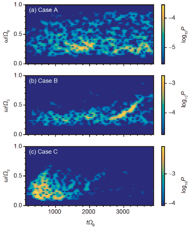
Figure 8: Contour plot of the whistler wave power spectrum (color bar) obtained by DAWN code [58] PIC simulations illustrating different qualitative behavior for increasing supra-thermal electron drive (From original figure in Ref. [60]). Case (A), (B) and (C), are characterized by the same parameters as in Fig. 1 except for $w_{\perp e}=0.32c$ (a), $w_{\perp e}=0.35c$ (b) and $w_{\perp e}=0.6c$ (c). Here, the original notation $\Omega_{0}$ stands for $\Omega_{e}$.

The first transition, according to the argument provided above and in Sec. 3.3 should be connected with the strength of linear drive; that is with the peak of the linear drive at $z=0$; i.e., $\gamma_{\rm max}$. In fact, noting Eq. (32) and neglecting, for simplicity, magnetic field non-uniformity vs. the non-uniformity of the energetic electron source (cf. Sec. 2), we have that the maximum amplification of the linear wave packet is [80]

$$I/I_{\omega 0} = \exp\left(2\int_{-\infty}^{\infty}\frac{\Gamma(z,0,\omega)}{v_{g}(z,\omega)}dz\right)$$

$$\simeq \exp\left(2\frac{\gamma_{\rm max}}{v_{g}(0,\omega)}\int_{-\infty}^{\infty}\zeta^{4}dz\right)=\exp\left(2\frac{\gamma_{\rm max}}{v_{g}(0,\omega)}\frac{\pi}{(A\xi)^{1/2}}\right)\;.$$

This suggest that $\gamma_{\rm max}$ should scale with $\xi^{1/2}$ to have the required minimum driving rate for successfully triggering chorus emission, as shown in Fig. 9 using DAWN code simulation results [58].

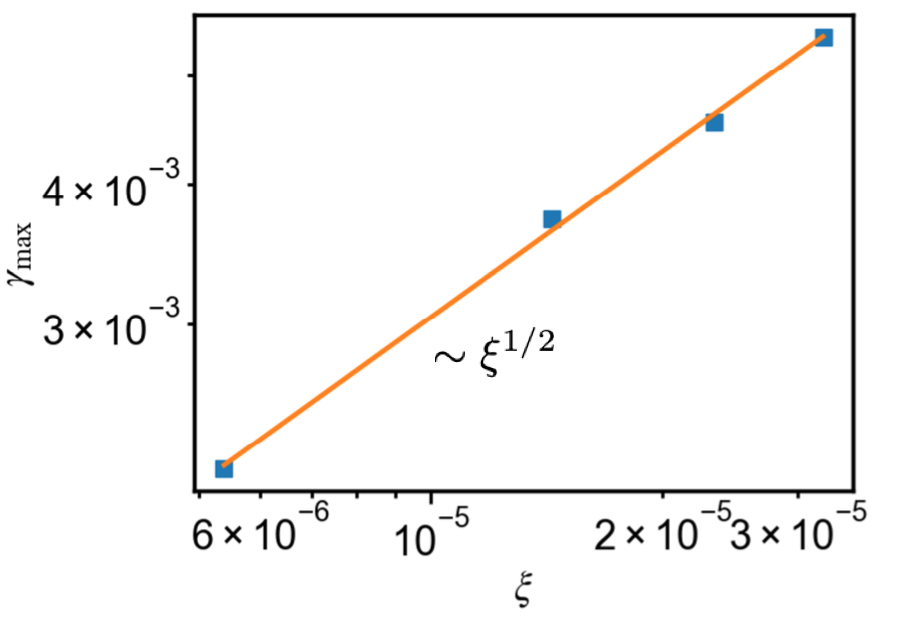
Figure 9: Scaling of the threshold in peak of the linear drive, $\gamma_{\rm max}$, with the magnetic field nonuniformity parameter, $\xi$, needed for chorus emission in DAWN code PIC simulations [58].

4.2 Reduced Dyson model for chorus emission: derivation

The derivation of the reduced Dyson model for chorus emission is originally given in Ref. [83]. It is beyond the intended scope of the present tutorial manuscript to enter into the same detailed analysis. We rather give a sketch of that derivation, which we try to make accessible to a broad readership, leaving interested readers to the original reference for details. As anticipated in the introductory remarks of Sec. 4, we can have a first simplification noting the $\sim\zeta^{4}\sim(1+A\xi z^{2})^{-2}$ scaling of Eq. (20), when the magnetic field non-uniformity is neglected; that is, when $\Omega\simeq\Omega_{e}$ and $\xi z^{2}\ll 1$ are assumed. This allows us to rewrite Eq. (18) as

$$W(z,t,\omega)+i\Gamma(z,t,\omega)=$$

$$\hskip 20.00003pt=\frac{\omega(\Omega_{e}-\omega)^{2}}{\Omega_{e}}\frac{n_{e}}{n}\zeta^{4}\left\langle\frac{v_{\perp}^{2}}{2}{\cal P}_{k}\left[\frac{kv_{\perp}^{2}}{2\omega}\frac{\partial\hat{f}_{0}}{\partial v_{\|}}-\frac{\Omega_{e}}{\omega}\hat{f}_{0}\right]_{k=K(z=0,\omega)}\right\rangle\;,$$ (72)

where we let $(1-kv_{\parallel}/\omega)\simeq\Omega_{e}/\omega$ for nearly resonant particles and $\hat{f}_{0}=f_{0}/n_{e}$ represents the normalized electron response computed for a uniform anisotropic plasma. Furthermore, all whistler wave dispersion relation and dispersive properties, including the ${\cal P}_{k}$ propagator defined in Eq. (61), are intended to be computed at $k=K(z=0,\omega)$ (cf. Sec. 2) [83]. For example, the integral operator defined in Eq. (28) becomes algebraic, $T_{\omega}(z)=z/v_{g\omega}$, and its inverse is also simplified, $T^{-1}_{\omega}(t)=v_{g\omega}t$, with $v_{g\omega}=v_{g}(z=0,\omega)$. Note that Eq. (72) is fully nonlinear, although the linear limit is readily recovered for ${\cal P}_{k}=[\Omega_{e}+kv_{\parallel}-\omega]^{-1}$ and $\hat{f}_{0}$ given by the properly rescaled bi-Maxwellian in Eq. (17). Following Ref. [83], it is also useful to introduce the rescaled phase shift and driving rate, $\bar{W}(z,t,\omega)$ and $\bar{\Gamma}(z,t,\omega)$, defined as

$$W(z,t,\omega)+i\Gamma(z,t,\omega)\equiv\zeta^{4}\frac{\omega(\Omega_{e}-\omega)^{2}}{\Omega_{e}^{2}(1-v_{r\omega}/v_{g\omega})^{2}}\left[\bar{W}(z,t,\omega)+i\bar{\Gamma}(z,t,\omega)\right]\;,$$ (73)

where $v_{r\omega}=v_{r}(z=0,\omega)$. As a result, Eq. (72) can be rewritten as

$$\bar{W}(z,t,\omega)+i\bar{\Gamma}(z,t,\omega)=\frac{n_{e}}{n}\left(1-\frac{v_{r\omega}}{v_{g\omega}}\right)^{2}\left\langle\Omega_{e}{\cal P}_{k}\left[\frac{kv_{\perp}^{2}}{2\omega}\frac{\partial}{\partial v_{\parallel}}-\frac{\Omega_{e}}{\omega}\right]\hat{f}_{0}\right\rangle\;.$$ (74)

Equation (74) hints at the reason underlying the construction of the reduced Dyson model; that is, we could readily solve the equations for the fluctuation spectrum, Eqs. (23) and (26), if we could determine $\bar{W}$ and $\bar{\Gamma}$ without solving for the whole phase space renormalized electron response, $\hat{f}_{0}$. This is the second simplification alluded at in the introduction to Sec. 4.

In order to make further analytic progress, let us consider $\hat{f}_{0}\equiv(\partial_{t}+v_{\parallel}\partial_{z})^{-1}(\partial_{t}+v_{\parallel}\partial_{z})\hat{f}_{0}$ on the right hand side of Eq. (74), and use Eq. (55) to rewrite $(\partial_{t}+v_{\parallel}\partial_{z})\hat{f}_{0}$ therein. The advantage of this formal manipulation will be clear later. We can also consider the nonlinear evolution of the whistler wave spectrum at one fixed $z$, chosen such that $z$ is outside the “hot” electron source region and, consistent with Eqs. (32) and (33) as well as Fig. 3, the fluctuation spectrum depends only on $t-z/v_{g\omega}$. In this way, we can focus on the nonlinear behaviors, separating them from those due to linear wave packet propagation. As a consequence, the same kind of dependence is reflected upon $\hat{f}_{0}$ and $\delta\hat{\bar{f}}_{k}\equiv\zeta^{-4}\delta\bar{f}_{k}/n_{e}$; that is, the rescaled supra-thermal electron response consistent with the earlier definition of $\hat{f}_{0}$. Note that, similar to $\hat{f}_{0}$, also $\delta\hat{\bar{f}}_{k}$ corresponds to electron response in uniform plasma, all spatial dependences being accounted for by the $\zeta^{4}$ factor in Eq. (73). Meanwhile, this simplified “local” limit is readily obtained from the more general case by replacing $(\partial_{t}+v_{\parallel}\partial_{z})\rightarrow(1-v_{r\omega}/v_{g\omega})\partial_{t}$ for nearly resonant particles [83].

Based on these assumptions, on the right hand side of Eq. (55) we can write

$$i\left(\delta\bar{E}_{k}{\cal P}_{k}^{*}\delta\bar{E}_{k}^{*}-\delta\bar{E}_{k}^{*}{\cal P}_{k}\delta\bar{E}_{k}\right)$$

$$\hskip 20.00003pt=i\left(\delta\bar{E}_{k}{\cal P}_{k}^{*}{\cal P}_{k}{\cal P}_{k}^{-1}\delta\bar{E}_{k}^{*}-\delta\bar{E}_{k}^{*}{\cal P}_{k}{\cal P}_{k}^{*}{\cal P}_{k}^{*-1}\delta\bar{E}_{k}\right)$$

$$\hskip 20.00003pt\simeq 2|\delta\bar{E}_{k}||{\cal P}_{k}|^{2}(1-v_{r\omega}/v_{g\omega})\partial_{t}|\delta\bar{E}_{k}|\;,$$ (75)

where, consistent with the optimal ordering for chorus excitation, Eq. (69), discussed in Sec. 3.3, we dropped resonance broadening [83]; and we introduced the notation

$${\cal P}_{k}^{*}{\cal P}_{k}\simeq{\cal P}_{k}{\cal P}_{k}^{*}\simeq|{\cal P}_{k}|^{2}=\left[(\Omega_{e}+kv_{\parallel}-\omega)^{2}+(1-v_{r\omega}/v_{g\omega})^{2}\partial_{t}^{2}\right]^{-1}\;.$$ (76)

Note that the operators action on the phase dependences in $\delta\bar{E}_{k}$ and its complex conjugate cancel out and only $\partial_{t}|\delta\bar{E}_{k}|$ survives. With help of these identities, and substituting Eq. (55) on the right hand side of Eq. (74), that equation can be cast as

$$\bar{W}(\omega)+i\bar{\Gamma}(\omega) = \frac{n_{e}}{n}\left(1-\frac{v_{r\omega}}{v_{g\omega}}\right)^{2}\left\langle\frac{v_{\perp}^{4}}{2}\Omega_{e}{\cal P}_{k}\left(\frac{k}{\omega}\frac{\partial}{\partial v_{\parallel}}-\frac{2}{\left\langle v_{\perp}^{2}\right\rangle}\frac{\Omega_{e}}{\omega}\right)\right.$$ (77)

$$\times(1-v_{r\omega}/v_{g\omega})^{-1}\partial_{t}^{-1}\sum_{k^{\prime}}\frac{e^{2}}{2m^{2}}|\delta\bar{E}_{k^{\prime}}|\frac{k^{\prime}}{\omega^{\prime}}\frac{\partial}{\partial v_{\parallel}}|{\cal P}_{k^{\prime}}|^{2}$$

$$\times(1-v_{r\omega^{\prime}}/v_{g\omega^{\prime}})\left.\partial_{t}|\delta\bar{E}_{k^{\prime}}|\left(\frac{k^{\prime}}{\omega^{\prime}}\frac{\partial}{\partial v_{\parallel}}-\frac{2}{\left\langle v_{\perp}^{2}\right\rangle}\frac{\Omega_{e}}{\omega^{\prime}}\right)\hat{f}_{0}\right\rangle.$$

Here, we have explicitly denoted only the frequency dependence of $\bar{W}$ and $\bar{\Gamma}$, and left implicit the dependence on $t-z/v_{g\omega}$. Furthermore, we have introduced the notation $\left\langle v_{\perp}^{2}\right\rangle\equiv\left\langle v_{\perp}^{2}\hat{f}_{0}\right\rangle/\left\langle\hat{f}_{0}\right\rangle$. Interested readers can find in Ref. [83] all technical details involved in the derivation of Eq. (77) from Eqs. (55) and (74). Velocity space integrals in Eq. (77) can be carried out assuming that the fluctuation spectrum is quasi-coherent (narrow) and representing operators in the Laplace space (cf., e.g., [78, 79, 11, 60]). Separating real and imaginary parts, and noting that, for nearly resonant particles,

$$\frac{1}{k}\frac{\partial}{\partial v_{\parallel}}\simeq\frac{1}{k}\frac{\partial}{\partial v_{r\omega}}=\frac{1}{(1-v_{r\omega}/v_{g\omega})}\frac{\partial}{\partial\omega}\;,$$ (78)

one can finally show, after lengthy but straightforward algebra [83]

$$\Omega_{e}^{-1}\partial_{t}\bar{W}(\omega) = \left[\Omega_{e}\frac{\partial}{\partial\omega}-\frac{2\Omega_{e}^{2}}{k^{2}\left\langle v_{\perp}^{2}\right\rangle}\left(1-\frac{v_{r\omega}}{v_{g\omega}}\right)\right]\Omega_{e}\frac{\partial}{\partial\omega}$$ (79)

$$\times\sum_{k^{\prime}}\frac{\left(\omega^{\prime}-\omega\right)}{2\Omega_{e}}\left[\frac{\left(\omega^{\prime}-\omega\right)^{2}}{4\Omega_{e}^{2}}+\Omega_{e}^{-2}\partial_{t}^{2}\right]^{-1}$$

$$\times\frac{\left\langle\left\langle\omega_{{\rm tr}k^{\prime}}^{4}\right\rangle\right\rangle}{4\Omega_{e}^{4}(1-v_{r\omega^{\prime}}/v_{g\omega^{\prime}})^{4}}\left(\frac{\bar{\Gamma}(\omega)+\bar{\Gamma}(\omega^{\prime})}{2}\right)\;,$$

where $\left\langle\left\langle\omega_{{\rm tr}k}^{4}\right\rangle\right\rangle=\left\langle v_{\perp}^{2}\omega_{{\rm tr}k}^{4}\hat{f}_{0}\right\rangle/\left\langle v_{\perp}^{2}\hat{f}_{0}\right\rangle$ is the velocity space averaged wave particle trapping frequency; and, defining $\bar{\Gamma}_{NL}=\bar{\Gamma}-\bar{\Gamma}_{L}$, with $\bar{\Gamma}_{L}$ the linear (initial) normalized hot electron driving rate,

$$\bar{\Gamma}_{NL}(\omega) = \left[\Omega_{e}\frac{\partial}{\partial\omega}-\frac{2\Omega_{e}^{2}}{k^{2}\left\langle v_{\perp}^{2}\right\rangle}\left(1-\frac{v_{r\omega}}{v_{g\omega}}\right)\right]\Omega_{e}\frac{\partial}{\partial\omega}$$ (80)

$$\times\sum_{k^{\prime}}\left[\frac{\left(\omega^{\prime}-\omega\right)^{2}}{4\Omega_{e}^{2}}+\Omega_{e}^{-2}\partial_{t}^{2}\right]^{-1}$$

$$\times\frac{\left\langle\left\langle\omega_{{\rm tr}k^{\prime}}^{4}\right\rangle\right\rangle}{4\Omega_{e}^{4}(1-v_{r\omega^{\prime}}/v_{g\omega^{\prime}})^{4}}\left(\frac{\bar{\Gamma}(\omega)+\bar{\Gamma}(\omega^{\prime})}{2}\right)\;.$$

Equations (79) and (80) have been significantly simplified with respect to the original Dyson-like equation, Eq. (55). Together with Eqs. (32) and (33), they provide the reduced Dyson model equations for chorus nonlinear dynamics and the most important novel result of [83]. Despite they are complicated nonlinear integro-differential equations, they allow us to understand the mechanism underlying chorus chirping. In fact, noting the optimal ordering of Eq. (69) introduced in Sec. 3.3, we expect that nonlinear behavior in Eqs. (79) and (80) may change when, in the first square parenthesis on the right hand side, $\Omega_{e}\partial_{\omega}$ dominates and, in the second square parenthesis, $(\omega^{\prime}-\omega)^{2}$ can be dropped with respect to $4\partial_{t}^{2}$. As a consequence of this and of the fact that gradients in the $\omega$ space are dominated by the nonlinear behavior, Eq. (80) becomes [83]

$$\frac{\partial^{2}}{\partial t^{2}}\bar{\Gamma}_{NL}(\omega)\simeq\left(\sum_{k^{\prime}}\frac{\left\langle\left\langle\omega_{\mathrm{tr}k^{\prime}}^{4}\right\rangle\right\rangle}{4\left(1-v_{r\omega^{\prime}}/v_{g\omega^{\prime}}\right)^{4}}\right)\frac{\partial^{2}}{\partial\omega^{2}}\bar{\Gamma}_{NL}(\omega)\;.$$ (81)

Equation (81) has a “self-similar solution that ballistically propagates in $\omega$-space at a rate given by the square root of the quantity in parentheses on the right hand side” [83]. Correspondingly, structures in the supra-thermal electron phase space also propagate at the same rate as described by the Dyson-like equation, Eq. (55) [11, 78, 79]. This process depends on the details of the fluctuation spectrum. However, for quasi-coherent chorus emission, we can simplify the first term on the right hand side of Eq. (81) noting that the spectrum of $\omega_{\mathrm{tr}k}^{4}=k^{2}v_{\perp}^{2}(e\delta\bar{B}_{ky}/mc)^{2}$ is much narrower than any characteristic widths due to $k=K(z=0,\omega)$ dependences in either group or phase velocities, as shown in Eq. (8). Thus,

$$\sum_{k^{\prime}}\frac{\left\langle\left\langle\omega_{\mathrm{tr}k^{\prime}}^{4}\right\rangle\right\rangle}{4\left(1-v_{r\omega^{\prime}}/v_{g\omega^{\prime}}\right)^{4}}\simeq\frac{\left\langle\left\langle(ekv_{\perp}/mc)^{2}\right\rangle\right\rangle}{4\left(1-v_{r\omega}/v_{g\omega}\right)^{4}}\sum_{k^{\prime}}\delta\bar{B}^{2}_{k^{\prime}y}$$

$$\hskip 20.00003pt\simeq\frac{\left\langle\left\langle(ekv_{\perp}/mc)^{2}\right\rangle\right\rangle}{4\left(1-v_{r\omega}/v_{g\omega}\right)^{4}}\delta\bar{B}^{2}_{ky}=\frac{\left\langle\left\langle\omega_{\mathrm{tr}k}^{4}\right\rangle\right\rangle}{4\left(1-v_{r\omega}/v_{g\omega}\right)^{4}}\;.$$

Here, we have noted that, from both observation and theory points of view, the magnetic fluctuation energy in a certain “narrow” $k$-spectrum range can be legitimately attributed to the reference $k$. Therefore, Eq. (81) can be rewritten as

$$\frac{\partial^{2}}{\partial t^{2}}\bar{\Gamma}_{NL}(\omega)\simeq\left(\frac{\partial\omega}{\partial t}\right)^{2}\frac{\partial^{2}}{\partial\omega^{2}}\bar{\Gamma}_{NL}(\omega)\;,$$ (82)

where

$$\frac{\partial\omega}{\partial t}=\pm\frac{1}{2}\frac{\left\langle\left\langle\omega_{\mathrm{tr}k}^{4}\right\rangle\right\rangle^{1/2}}{\left(1-v_{r\omega}/v_{g\omega}\right)^{2}}\;;$$ (83)

and the corresponding “self-similar” solution is $\bar{\Gamma}_{NL}(\omega-(\partial\omega/\partial t)t)$, demonstrating its ballistic propagation in $\omega$-space at the rate given by Eq. (83). This results is the analytic proof of the well-known Vomvoridis expression of chorus chirping [72], with $|R|=1/2$ in Eq. (42) neglecting magnetic field non-uniformity, based on the conjecture of maximized wave particle power transfer and PIC simulation results. Very similar chirping rates as in [72] have also been obtained by [67, 44]. Equations (81) and (83), originally derived in [83], demonstrate that chorus chirping is indeed obtained by maximization of spontaneous fluctuation growth; i.e., maximization of wave particle power transfer [11, 78, 79]. They predict that chorus can be rising- as well as falling-tone, consistent with [75]; thus, suggesting that the motivation of rising-tone chorus prevalence is due to the second term in the first square parenthesis on the right hand side in Eqs. (79) and (80), or other symmetry breaking effects (cf. next subsection). Other possible explanations rely on the magnetic field non-uniformity [75, 61], which is neglected in the present simplified analysis. Interested readers are referred to original works for more details. Another important feature of Eq. (81) is that it shows that the chorus chirping rate depends on the fluctuation spectrum and reduces to $|R|=1/2$ only for a nearly monochromatic spectrum [83]. In other words, the actual value of chorus chirping may depend on the initial hot electron distribution function and other excitation conditions. Undoubtedly, for the conditions of Eq. (81) to be derived from Eq. (80), phase space structures must exist in the supra-thermal electron phase space; that is, $|R|<1$ is a stringent condition as discussed in Sec. 3.1.

4.3 Reduced Dyson model for chorus emission: numerical solution

In this subsection, we numerically solve the reduced Dyson model equations schematically presented above, following the original derivation in [83]. For the sake of convenience, we will treat the whistler wave fluctuation spectrum as a continuum, although Eqs. (79) and (80) have been derived assuming a generic discrete fluctuation spectrum, including a single mode as limiting case. For this, we introduce the normalized spectral density ${\cal I}(\omega)$ defined as [83]

$$\sum_{k}\frac{\left\langle\left\langle\omega_{trk}^{4}\right\rangle\right\rangle}{\Omega_{e}^{4}}=\sum_{k}\frac{\left\langle\left\langle k^{3}v_{\perp}^{2}\right\rangle\right\rangle}{\Omega_{e}^{2}}\frac{I_{k}}{4B_{e}^{2}}\equiv\frac{\hat{\gamma}_{e}^{2}}{\Omega_{e}^{2}}\int\frac{d\omega}{\Omega_{e}}\mathcal{I}(\omega)\frac{\omega^{3/2}}{\left(\Omega_{e}-\omega\right)^{3/2}}\;,$$ (84)

where $\hat{\gamma}_{e}$ is the peak value of the linear hot electron driving rate at the equator and normalizations are chosen such that nonlinearity effects become important when ${\cal I}(\omega)\sim{\cal O}(1)$. As in Sec. 4.2, only dependences on $\omega$ are explicitly given, while dependences on $t-z/v_{g\omega}$ are implicitly assumed for notation simplicity. To practically solve the integral operators in the reduced Dyson model equations, let us introduce the auxiliary functions

$$\left[\frac{\left(\omega-\omega^{\prime}\right)^{2}}{4\Omega_{e}^{2}}+\Omega_{e}^{-2}\partial_{t}^{2}\right]G_{L1}(\omega,\omega^{\prime})=\frac{\hat{\gamma}_{e}^{2}}{\Omega_{e}^{2}}\frac{{\cal I}(\omega)}{(1-v_{r\omega}/v_{g\omega})^{4}}\bar{\Gamma}_{L}(\omega)\;,$$

$$\left[\frac{\left(\omega-\omega^{\prime}\right)^{2}}{4\Omega_{e}^{2}}+\Omega_{e}^{-2}\partial_{t}^{2}\right]G_{L2}(\omega,\omega^{\prime})=\frac{\hat{\gamma}_{e}^{2}}{\Omega_{e}^{2}}\frac{{\cal I}(\omega)}{(1-v_{r\omega}/v_{g\omega})^{4}}\bar{\Gamma}_{L}(\omega^{\prime})\;,$$

$$\left[\frac{\left(\omega-\omega^{\prime}\right)^{2}}{4\Omega_{e}^{2}}+\Omega_{e}^{-2}\partial_{t}^{2}\right]G_{NL1}(\omega,\omega^{\prime})=\frac{\hat{\gamma}_{e}^{2}}{\Omega_{e}^{2}}\frac{{\cal I}(\omega)}{(1-v_{r\omega}/v_{g\omega})^{4}}\bar{\Gamma}_{NL}(\omega)\;,$$

$$\left[\frac{\left(\omega-\omega^{\prime}\right)^{2}}{4\Omega_{e}^{2}}+\Omega_{e}^{-2}\partial_{t}^{2}\right]G_{NL2}(\omega,\omega^{\prime})=\frac{\hat{\gamma}_{e}^{2}}{\Omega_{e}^{2}}\frac{{\cal I}(\omega)}{(1-v_{r\omega}/v_{g\omega})^{4}}\bar{\Gamma}_{NL}(\omega^{\prime})\;;$$ (85)

which let us rewrite Eq. (80) and Eq. (79) respectively as

$$\bar{\Gamma}_{NL}(\omega) = \left[\Omega_{e}\frac{\partial}{\partial\omega}-\frac{2\Omega_{e}^{2}}{k^{2}\left\langle v_{\perp}^{2}\right\rangle}\left(1-\frac{v_{r\omega}}{v_{g\omega}}\right)\right]\Omega_{e}\frac{\partial}{\partial\omega}\int\frac{d\omega^{\prime}}{\Omega_{e}}\frac{\omega^{\prime 3/2}}{(\Omega_{e}-\omega^{\prime})^{3/2}}$$ (86)

$$\times\frac{1}{8}\left(G_{L1}(\omega^{\prime},\omega)+G_{L2}(\omega^{\prime},\omega)+G_{NL1}(\omega^{\prime},\omega)+G_{NL2}(\omega^{\prime},\omega)\right);$$

and

$$\Omega_{e}^{-1}\partial_{t}\bar{W}(\omega) = \left[\Omega_{e}\frac{\partial}{\partial\omega}-\frac{2\Omega_{e}^{2}}{k^{2}\left\langle v_{\perp}^{2}\right\rangle}\left(1-\frac{v_{r\omega}}{v_{g\omega}}\right)\right]\Omega_{e}\frac{\partial}{\partial\omega}\int\frac{d\omega^{\prime}}{\Omega_{e}}\frac{\omega^{\prime 3/2}}{(\Omega_{e}-\omega^{\prime})^{3/2}}$$ (87)

$$\times\frac{\left(\omega^{\prime}-\omega\right)}{16\Omega_{e}}\left(G_{L1}(\omega^{\prime},\omega)+G_{L2}(\omega^{\prime},\omega)+G_{NL1}(\omega^{\prime},\omega)+G_{NL2}(\omega^{\prime},\omega)\right).$$

Recalling that we are focusing on the normalized spectral density evolution at fixed $z$ outside the hot electron source region, Eqs. (85) to (87) can be closed by the intensity evolution equation,

$$\Omega_{e}^{-1}\partial_{t}{\cal I}(\omega) = 2{\cal S}{\cal I}(\omega)^{1/2}+2{\cal I}(\omega)\frac{\omega(\Omega_{e}-\omega)^{2}}{\Omega_{e}^{3}}\left[\partial_{t}\left(\int_{z-v_{g\omega}t}^{\infty}\zeta^{4}(z^{\prime})\frac{dz^{\prime}}{v_{g\omega}}\right)\bar{\Gamma}(\omega)\right.$$ (88)

$$\left.\left.+\left(\int_{z-v_{g\omega}t}^{\infty}\zeta^{4}(z^{\prime})\frac{dz^{\prime}}{v_{g\omega}}\right)\partial_{t}\bar{\Gamma}(\omega)\right]\right/\left(1-\frac{v_{r\omega}}{v_{g\omega}}\right)^{2}\;;$$

and the wave packet phase evolution equation,

$$\Omega_{e}^{-1}\partial_{t}\varphi(\omega) = -\frac{\omega(\Omega_{e}-\omega)^{2}}{\Omega_{e}^{3}}\left[\partial_{t}\left(\int_{z-v_{g\omega}t}^{\infty}\zeta^{4}(z^{\prime})\frac{dz^{\prime}}{v_{g\omega}}\right)\bar{W}(\omega)\right.$$ (89)

$$\left.\left.+\left(\int_{z-v_{g\omega}t}^{\infty}\zeta^{4}(z^{\prime})\frac{dz^{\prime}}{v_{g\omega}}\right)\partial_{t}\bar{W}(\omega)\right]\right/\left(1-\frac{v_{r\omega}}{v_{g\omega}}\right)^{2}\;;$$

which can be readily derived from Eqs. (23) and (26) noting Eq. (34) and the analogous identity that one can write for $\partial_{t}\varphi$ [83]. On the right hand side of Eq. (88), we have added a source term $2{\cal S}{\cal I}(\omega)^{1/2}$, representing the injection rate of fluctuations in the $|\delta\bar{E}_{k}|$ spectrum. In the absence of supra-thermal electrons, the effect of a constant source would give an intensity spectrum ${\cal I}={\cal S}^{2}\Omega_{e}^{2}t^{2}$, corresponding to $|\delta\bar{E}_{k}|$ linearly increasing with time. This choice gives us a variety of possibilities rather than assuming an initial spectrum. Since Ref. [83] demonstrated that there are no qualitative differences between using ${\cal S}$ as a random source stirring the system or a constant uniform source in frequency, we focus, here, on the uniform source case.

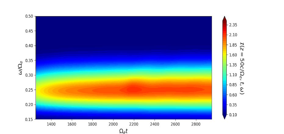
(a)

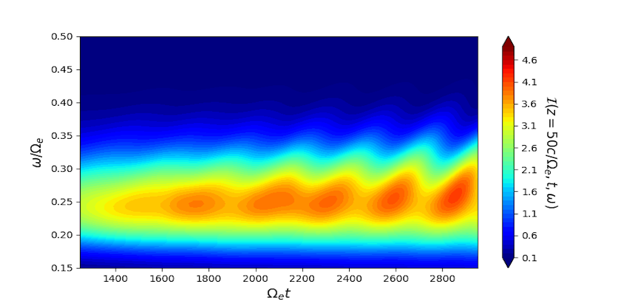
(b)

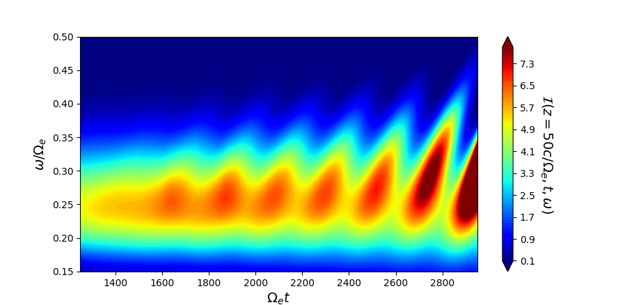
(c)

Figure 10: Contour plots in the $(\Omega_{e}t,\omega/\Omega_{e})$ space of the nonlinear evolution of the fluctuation spectrum for the same physical parameters as in Fig. 1. Position is fixed at $z\Omega_{e}/c=50$, outside the hot electron source region. From top to bottom, the uniform (in $\omega$ space) source, ${\cal S}$ in Eq. (88), increases: ${\cal S}=1\times 10^{-5}$ [case (a)], ${\cal S}=\sqrt{2}\times 10^{-5}$ [case (b)], and ${\cal S}=2\times 10^{-5}$ [case (c)]. The existence of a lower threshold for the onset of chorus chirping (cf. Sec. 4.1) is evident when going from case (a) to case (b).

When solving Eqs. (86) to (89) by advancing them in time by one step $\Delta t$, it is necessary to keep into account frequency ($\Delta_{\omega}=-\partial_{t}\varphi(\omega)$) and wave number ($\Delta_{k}$) shifts. Consistent with the analysis of Sec. 2, $\Delta_{\omega}/\Delta_{k}=v_{g\omega}$ and the nonlinearly shifted wave packet still satisfies the whistler dispersion relation. However, there exists a corresponding small but finite shift in the resonant velocity $k\Delta v_{r\omega}=\Delta_{\omega}-v_{r\omega}\Delta_{k}=(1-v_{r\omega}/v_{g\omega})\Delta_{\omega}$. Thus, after advancing by one step $\Delta t$, the functions $\bar{\Gamma}_{NL}$ and $\bar{W}_{NL}$ are actually evaluated at $\omega+\Delta(\Delta_{\omega})$, with $\Delta(\Delta_{\omega})=-\Delta t\partial_{t}^{2}\varphi(\omega)$, and, noting Eq. (78), these functions have to be updated as

$$\bar{\Gamma}_{NL}(\omega) \rightarrow \bar{\Gamma}_{NL}(\omega)-\Delta(\Delta_{\omega})\frac{\partial}{\partial\omega}\bar{\Gamma}_{NL}(\omega)\;,$$

$$\bar{W}_{NL}(\omega) \rightarrow \bar{W}_{NL}(\omega)-\Delta(\Delta_{\omega})\frac{\partial}{\partial\omega}\bar{W}_{NL}(\omega)\;.$$ (90)

The same argument evidently applies to ${\cal I}(\omega)$ and $\varphi(\omega)$, such that

$${\cal I}(\omega) \rightarrow {\cal I}(\omega)-\Delta(\Delta_{\omega})\frac{\partial}{\partial\omega}{\cal I}(\omega)\;,$$

$$\varphi(\omega) \rightarrow \varphi(\omega)-\Delta(\Delta_{\omega})\frac{\partial}{\partial\omega}\varphi(\omega)\;;$$ (91)

after each time step. Equation (91) corresponds to changing $\partial_{t}\rightarrow\partial_{t}-\partial_{t}^{2}\varphi(\omega)\partial_{\omega}$ on the left hand side of Eqs. (88) and (89); which corresponds to solving the wave kinetic equation [7, 34] for wave packet intensity and phase. Initial conditions are homogeneous; that is, ${\cal I}(\omega)=0$ together with $\varphi(\omega)=0$ at $t=0$, as well as $\left.G_{...}(\omega^{\prime},\omega)\right|_{t=0}=0$ and $\left.\partial_{t}G_{...}(\omega^{\prime},\omega)\right|_{t=0}=0$ on all auxiliary functions introduced in Eqs. (85). Meanwhile, solutions at the boundaries of the considered interval in $\omega$ space are obtained by linear extrapolation of the inner solution.

For the same physical parameters of Fig. 1, and assuming fixed $z\Omega_{e}/c=50$, the nonlinear evolution of ${\cal I}(z=50c/\Omega_{e},t,\omega)$ is shown in Fig. 10 for ${\cal S}=1\times 10^{-5}$ [case (a)], ${\cal S}=\sqrt{2}\times 10^{-5}$ [case (b)], and ${\cal S}=2\times 10^{-5}$ [case (c)]. Here, we use a discretization in $\omega$ space with $221$ grid points in the interval $\omega/\Omega_{e}\in[0.05,0.9]$ and adopt, for cases (a) and (b), a Savitzky–Golay filter fitting sub-sets of 15 adjacent data points with a fourth order degree polynomial to ensure regularity of the derivatives in $\omega$-space. Case (c) uses fitting sub-sets of 19 adjacent data points to show that no significant changes are obtained by varying the Savitzky–Golay filter parameters. A fourth order Runge-Kutta integration in time is adopted with variable time step, gradually decreasing from an initial $\Omega_{e}\Delta t=1.25\times 10^{-1}$ in the early linear evolution to $\Omega_{e}\Delta t=3.125\times 10^{-2}$ in the later nonlinear phase at $\Omega_{e}t>1750$. This choice ensures that Courant condition is well satisfied. The routine solving Eqs. (85) to (89), closed by Eqs. (90) and (91) together with the aforementioned boundary conditions, is written in Python and uses Python standard libraries. Increasing ${\cal S}$ as in Fig. 10 helps clarifying the role of driving strength for triggering chorus emission; i.e., of the combination of convective amplification and initial intensity of the whistler wave packet. A clear “lower threshold” is crossed from panel (a) to (b): in the former case, nonlinear oscillations dominate the fluctuation spectrum evolution; while in the latter case, chorus elements are evidently produced. Figure 10, obtained by solution of the reduced Dyson model, is consistent with the PIC simulation results of Fig. 8 since, for the sake of simplicity, we have neglected resonance broadening and, thus, we do not expect chorus emission be smeared out by further increasing the driving strength.

Focusing on frequency chirping, Fig. 11 shows: (a) the chorus element starting at $\Omega_{e}t\sim 3000$ for case ${\cal S}=\sqrt{2}\times 10^{-5}$; and (b) the chorus element starting at $\Omega_{e}t\sim 2600$ for case ${\cal S}=2\times 10^{-5}$.

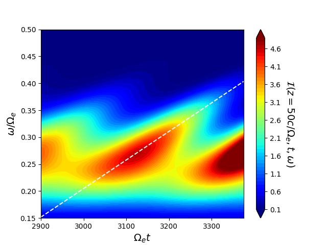
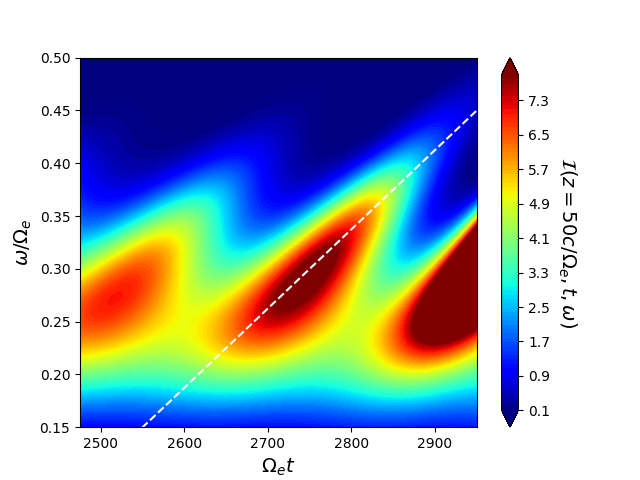
(a)                                                             (b)

Figure 11: Frequency chirping of individual chorus elements for ${\cal S}=\sqrt{2}\times 10^{-5}$ (a) and ${\cal S}=2\times 10^{-5}$ (b). The white dashed lines passing through the chorus elements represent the average chirping rate: $\partial_{t}\omega_{0}=5.3\times 10^{-4}$ (a) and $\partial_{t}\omega_{0}=7.5\times 10^{-4}$ (b).

The average chirping rate can be estimated as the average slope of a line fitting through the chorus element. It corresponds to the instantaneous chirping rate becoming essentially constant after the intensity peak in the chorus element is reached. It is $\partial_{t}\omega_{0}=5.3\times 10^{-4}$ for ${\cal S}=\sqrt{2}\times 10^{-5}$ and coincides with the value reported by PIC code simulations with DAWN code for the same parameters [59]. For ${\cal S}=2\times 10^{-5}$, the average chirping rate $\partial_{t}\omega_{0}=7.5\times 10^{-4}$, consistent with Eq. (83). The behavior of the instantaneous chirping rate is reported in Fig. 12. The average values, $\partial_{t}\omega_{0}=5.3\times 10^{-4}$ (a) and $\partial_{t}\omega_{0}=7.5\times 10^{-4}$ (b), are clearly recognizable.

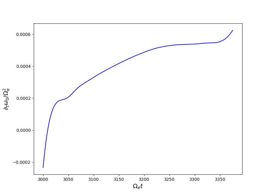
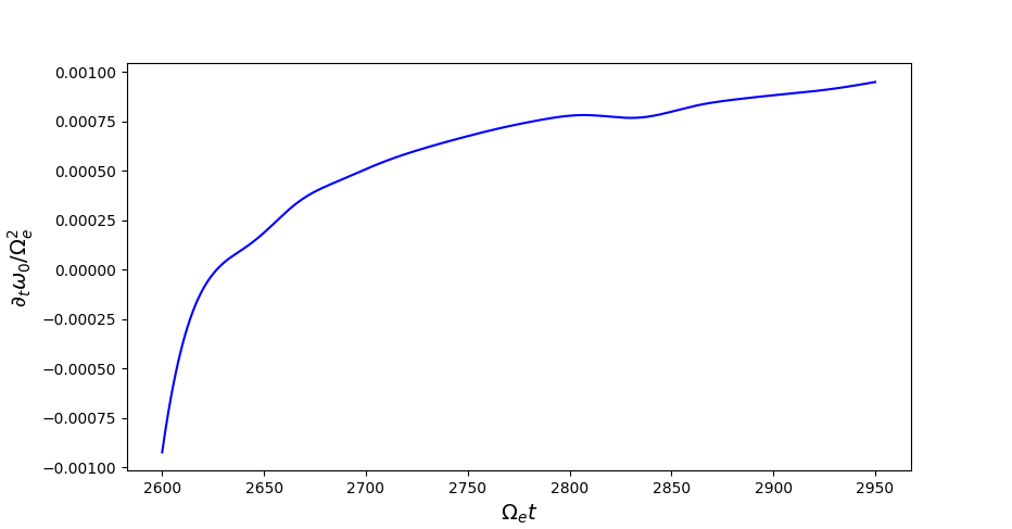
(a)                                                             (b)

Figure 12: Instantaneous chirping rate of the same chorus elements as in Fig. 11: for ${\cal S}=\sqrt{2}\times 10^{-5}$ (a) and ${\cal S}=2\times 10^{-5}$ (b).

That instantaneous values of frequency chirping start from negative values in both cases is consistent with Eq. (83) and Ref. [75]; and confirms that symmetry breaking that leads to the prevalence of rising tone chorus is due to the second term in the first square parenthesis on the right hand side in Eqs. (79) and (80), as argued in Sec. 4.2, or other effects such as the frequency asymmetry of the driving rate about its maximum, shown in Fig. 1(b). Further reasons of symmetry breaking, connected with the non-uniformity of the background magnetic field are discussed in [22, 56, 75, 61] and are beyond the scope of the present analysis. We refer interested readers to the original works.

Nonlinear dynamics in one single chorus elements are due to maximization of wave particle power transfer and intensity growth, as discussed in Sec. 4.2 and expected for a spontaneous process [78, 79, 11, 83]. Using the diagrammatic representation introduced in Figs. 5 and 6, this process may be represented as in Fig. 13 [83].

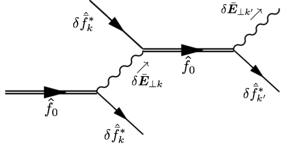
Figure 13: Diagrammatic representation of chorus chirping consistent with Figs. 5 and 6 (adapted from the original figure from Ref. [83]). The double solid line propagator indicates the hot electron renormalized response, which is unstable and spontaneously emits and reabsorbs most likely same-$k$ fluctuations corresponding to fluctuation spectrum instantaneous peak. Chorus chirping occurs because different $k$’s maximize wave particle power transfer at different times [80, 83].

This is further demonstrated in Fig. 14, where (a) provides the contour plot of the nonlinear frequency shift $\Delta_{\omega}(z=50c/\Omega_{e},t)$, while (b) shows the snapshot of the same quantity at $\Omega_{e}t=3125$. Here, we focus on the case at ${\cal S}=\sqrt{2}\times 10^{-5}$, since the detailed analysis of ${\cal S}=2\times 10^{-5}$ is given in [83]. Figure 14 clearly shows that $\Delta_{\omega}$ is always much smaller than the dynamic range of frequency chirping, demonstrating that individual oscillators in the whistler spectrum during a chorus event follow the well-know behavior of wheat explained by Leonardo Da Vinci:

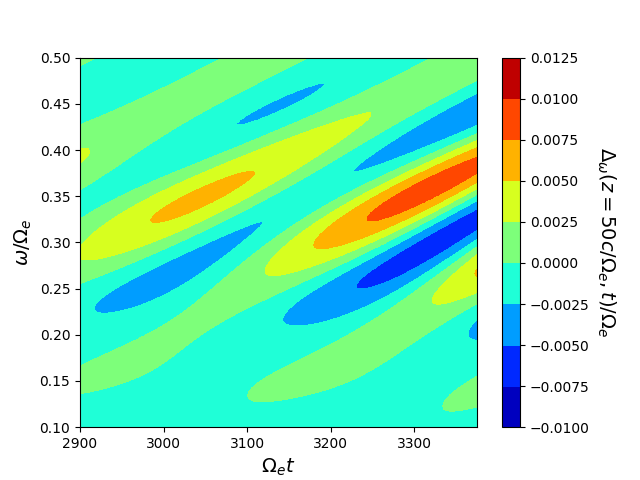
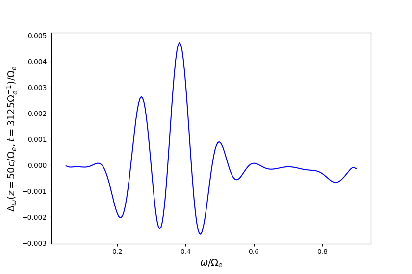
(a)                                                             (b)

Figure 14: Contour plot of the nonlinear frequency shift $\Delta_{\omega}(z=50c/\Omega_{e},t)$ (a) and snapshot of the same quantity at $\Omega_{e}t=3125$ (b) for the case ${\cal S}=\sqrt{2}\times 10^{-5}$ considered in Fig. 11.

Accade sovente che l’onda si allontani dal suo punto di creazione,

mentre l’acqua non si muove, come le onde create dal vento

in un campo di grano, dove vediamo le onde correre attraverso il campo

mentre il grano rimane al suo posto

It often happens that waves travel away from their creation point,

while water does not move, like waves created by wind

in a wheat field, where we see waves running across the field

while wheat remains in place

The chorus element is the “running wave” and Fig. 15 illustrates the time behavior of its peak intensity, ${\cal I}_{0}(z=50c/\Omega_{e},t)$, and corresponding nonlinear phase shift, $\Delta\varphi_{0}(z=50c/\Omega_{e},t)$, measured from the start of the considered time interval. We will come back to this figure in Sec. 5. Here, it is worthwhile noting that the maximum of the intensity is reached when $\Delta\varphi_{0}\simeq-\pi$ and that the nonlinear time change in fluctuation intensity is also reflected by the similar change in space, due to the dependence of ${\cal I}$ on $t-z/v_{g\omega}$. The same behavior is obtained for ${\cal S}=2\times 10^{-5}$ [83].

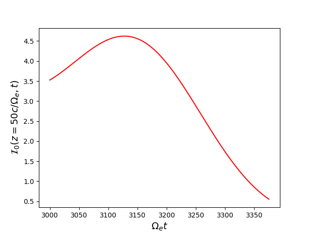
(a)                                                             (b)

Figure 15: Peak intensity, ${\cal I}_{0}(z=50c/\Omega_{e},t)$ (a), and corresponding nonlinear phase shift $\Delta\varphi_{0}(z=50c/\Omega_{e},t)$ (b), of the chorus element starting at $\Omega_{e}t\sim 3000$ for the case ${\cal S}=\sqrt{2}\times 10^{-5}$ considered in Fig. 11.

4.4 Comparison with other models of chorus chirping

The comparison with the analysis of chorus chirping originally proposed by [72] has been extensively provided in the previous subsections. One of the merits of the present theoretical framework is the analytical derivation, Eq. (83), of the optimal condition for wave particle power transfer, consistent with the conjecture of Ref. [72] based on PIC simulation results. We have also briefly analyzed the role of background magnetic field non-uniformity, originally discussed by [22, 56] and more recently revisited by [75, 61]. What may seem in apparent contrast with the present theoretical analysis is the interpretation of chorus frequency chirping given by [43], explained as consequence of the nonlinear current parallel to the wave magnetic field ($J_{B}$), responsible of nonlinear frequency shift. In particular, a sequence of “whistler seeds” that are excited and amplified by wave particle resonant interactions are at origin of frequency chirping.

Within the present theoretical framework, the fluctuation spectrum is self-consistently evolved and Fig. 14 demonstrates that each oscillator in the wave spectrum (each “wheat plant” in Leonardo’s metaphor; cf. Sec. 4.3) is characterized by a small nonlinear frequency shift. However, continuing the metaphor, when the “running wave” crosses the field while wheat remains in place, each wheat plant swings in tune with the wave when it is passed by the fluctuation peak. This also occurs for the chorus elements and it is shown in Fig. 16(a), where

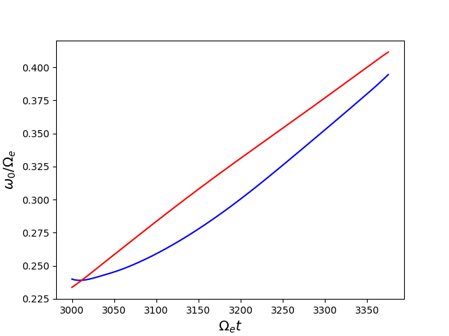
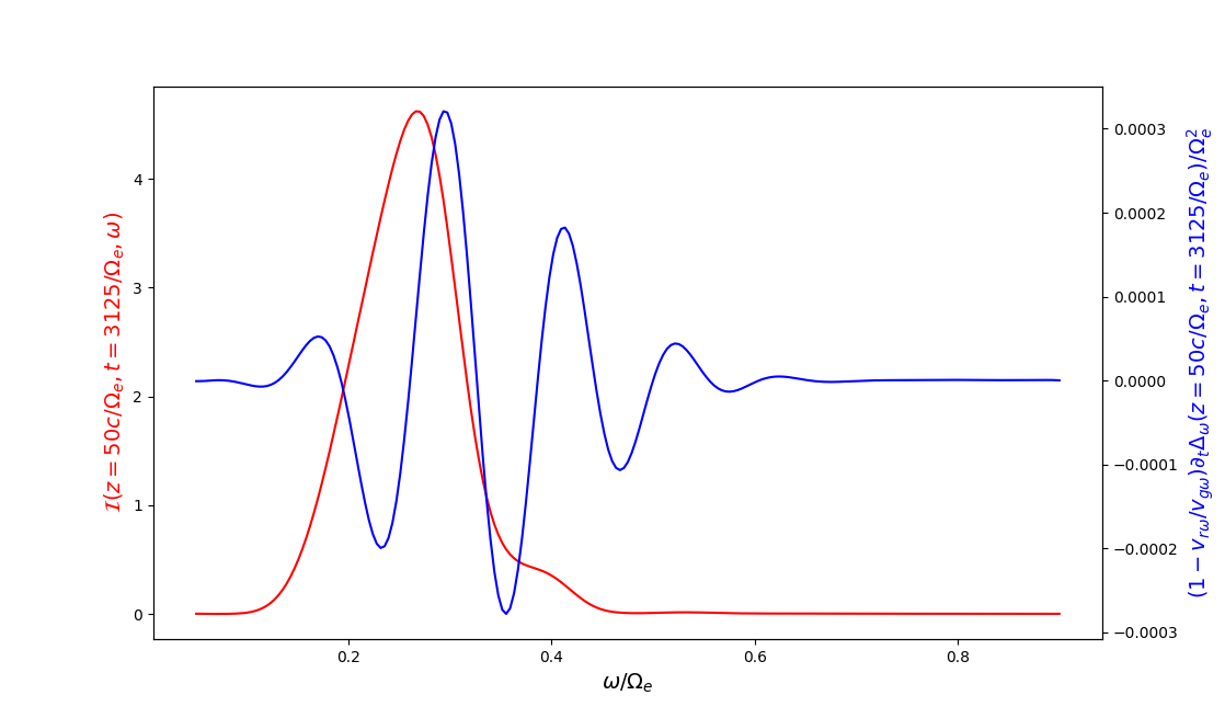
(a)                                                              (b)

Figure 16: (a) Time evolution of the intensity peak frequency (blue line) of the chorus element analyzed in Fig. 15. The red line denotes the frequency evolution of the maximum in the rate of change of nonlinear frequency shift. (b) Snapshot at $\Omega_{e}t=3125$ of the fluctuation intensity and of the $\partial_{t}\omega_{\rm res}=(1-v_{r\omega}/v_{g\omega})\partial_{t}\Delta_{\omega}$ as a function of frequency.

the time evolution of the intensity peak frequency of the chorus element analyzed in Fig. 15 is represented by the blue line. The red line, meanwhile denotes the frequency evolution of the maximum in the rate of change of nonlinear frequency shift. The connection between the frequencies of these two peaks is also shown in Fig. 16(b), providing the snapshot at $\Omega_{e}t=3125$ of the fluctuation intensity and of $\partial_{t}\omega_{\rm res}=(1-v_{r\omega}/v_{g\omega})\partial_{t}\Delta_{\omega}$ as a function of frequency. Recalling the discussion preceding Eq. (90), $\partial_{t}\omega_{\rm res}$ represents the rate of change of the resonance frequency. In conclusion, if one interprets the “whistler seeds” of [43] as the individual oscillators in the wave packet at the intensity peak, one should obtain the frequency increase due to the chorus chirping as

$$\Delta\omega=\int(1-v_{r\omega_{0}(t^{\prime})}/v_{g\omega_{0}(t^{\prime})})\partial_{t^{\prime}}\Delta_{\omega_{0}(t^{\prime})}dt^{\prime}\;,$$

where integration is to be intended along the red line of Fig. 16 (a) [83]. The hence obtained frequency increase is $\Delta\omega/\Omega_{e}=0.121$ over the considered time interval, against the corresponding frequency shift, $\Delta\omega/\Omega_{e}=0.155$, of the intensity peak. We believe that this good agreement confirms the present explanation that reconciles the original interpretation of frequency chirping given by [43] with the present theoretical analysis.

As a final remark, we would like to briefly comment about the recent work by [69], discussing Van Allen Probe data and showing that each chorus element is made of discrete sub-elements with constant frequency. The present theoretical framework, and Fig 14 in particular, supports that each oscillator in the whistler wave spectrum has a nonlinear frequency shift in the order of a few percent, consistent with observations by [69]. The discrete steps, which are the essential elements of the rising tone chorus element in this recent work, are instead beyond the description of the present theoretical analysis of the reduced Dyson model equations since, by definition in Eq. (84) and for the sake of simplicity, we assume the continuous limit. However, adopting the general theoretical framework discussed in Sec. 3, it would be possible to solve the self-consistent evolution equations for the fluctuation spectrum in any arbitrary discretized form. This approach would, thus, allow us to address the conditions described in [69]. Doing so is, however, beyond the scope of the tutorial style of the present work.

For the sake of completeness, we also mention the recent and extensive analysis by [77, 76], which provides statistical results from 6 years of Van Allen Probes data on the value of $\partial\omega/\partial t$ inside chorus wave packets. Unlike Ref. [69], [77, 76] show that the frequency variation inside long packets ($>50$ wave periods) is generally non-null and consistent with the usual chirping rate of [72, 44] and the present Eq. (83). These statistical observations have been recovered in numerical simulation results by [41]. Meanwhile, for very short packets ($<10$ wave periods), the results by [77, 76] agree with earlier works that attribute frequency chirping to nonlinear wave-particle interactions and wave superposition for moderate amplitudes [29, 14].

5 Discussion and conclusions

The physics processes connected with chorus emission, discussed in the previous sections, are so deeply rooted in fundamental elements of nonlinear dynamics and phase space transport that one may naturally expect many points of contact with similar phenomena occurring in space and laboratory plasmas. Following the intended scope of the present work, we will concentrate on the latter, discussing briefly examples from free electron lasers (FEL) and magnetic confinement fusion (MCF). Readers who may be interested in a somewhat “unconventional” perspective on fusion, triggered by collapsing whistler waves, are referred to the recent work by [49].

Analogies and similarities of chorus emission and FEL physics was noted and addressed in Ref. [54]. Here, we follow Refs. [78, 79, 11] and the more recent Ref. [61, 83] and draw analogies with FEL super-radiance [8, 9, 21, 73]. The dynamic evolution of intensity peak and phase of the chorus element in Fig. 15 correspond to synchronization (cf. Ref. [18]) of supra-thermal electrons and subsequent detuning as the chorus wave packet slips over the resonant electron population. During synchronization, phase evolution is minimized so that wave particle power extraction is maximum. While resonant particles release their energy to the wave, by moving from the positive to negative $\dot{\phi}$ domain in Fig. 4 as discussed in Sec. 4.1, peak intensity grows and phase gradually reaches $-\pi$. Resonance detuning, then, becomes relevant and is made more significant by the drop in fluctuation intensity. The analogies between these phases taking place during a chorus element and nonlinear pulse evolution in seeded FEL amplifiers, respectively, are further clarified by direct comparison of simulation results discussed in Fig. 6 of Ref. [61] and Fig. 3 of Ref. [21]. The main and most significant difference between chorus emission in planetary magnetospheres and FEL super-radiance is that the former is a spontaneous process, while the latter is stimulated or externally controlled. Interested readers are referred to original works for further details. In addition to this, it is worthwhile mentioning that parametric whistler wave generation during laser-plasma interaction have been addressed by [38]. We also note that the theoretical approaches presented in this work may also be applied toward in-depth understandings of the nonlinear phenomena in high power radiation devices such as gyrotron backwave oscillators [12, 13].

The strong connection of physics processes underlying chorus emission and various phenomena observed in MCF is actually one of the primary motivations of the present work, as mentioned in the Introduction. Magnetized plasmas of fusion interest are, in fact, the natural environment where a number of spontaneous frequency sweeping phenomena occur, since fluctuations of the shear Alfvén wave spectrum are strongly excited by resonant supra-thermal particles, notably charged fusion products and/or particles accelerated by additional heating systems [78, 79, 11]. For low-frequency fluctuations (below the ion-cyclotron frequency), self-consistent single-particle nonlinear dynamics in MCF plasmas reduces to a non-autonomous system with two degrees of freedom, while the same problem in the chorus case is well described by a non-autonomous system with one degree of freedom. In addition to this, the complex toroidal geometry and the nonlocal plasma response in MCF require analyzing the fluctuation spectrum evolution by means of a nonlinear Schrödinger-like equation (NLSE) [78, 79, 11], well beyond the wave kinetic equation paradigm [82]. The systematic development for MCF of the same theoretical framework presented in Sec. 3 has been carried out by [78, 79, 11] and, more recently, Ref. [19], leading to the so-called Dyson-Schrödinger Model (DSM) for transport in MCF [82]. The aforementioned complexities due to number of degrees of freedom and equilibrium geometry require a more systematic numerical approach to the solution of general governing equations. Notwithstanding these complications, solutions of simple limits in cases of practical interest have been obtained, such as for Energetic Particle Modes (EPM) [79] and fishbones [11]. In these cases, in particular, the existence of self-similar structures characterized by ballistic propagation in phase space establishes a fundamental connection between chorus and EPM as well as fishbone frequency chirping in MCF [11, 79]. In fact, the predicted propagation speed of these resonant structures scales linearly with the phase space velocity (and fluctuation amplitude) in the “resonant action” direction; that is, velocity (and/or frequency) for chorus and canonical angular momentum for EPM/fishbone. Interested readers may find a recent and in depth review of these analyses in Ref. [11].

As a final remark of this short trip through chorus physics, taken aboard the comfortable environment of plasma theory, we would like to note that windows were opened with a view over existing problems of both academic interest and practical implications. The mathematical language in which these problems are formulated are the Dyson Schwinger Equation (DSE) (cf. e.g. [27]) and NLSE. This naturally opens points of contact with condensed matter physics and more. The peculiar feature of collisionless plasmas to be characterized by nonlocal response in space and time gives to nonlinearities in these equations an intrinsic integral nature and is cause of a practically infinite variety of interesting behaviors. This is ultimately what makes plasma physics such an exciting cross-disciplinary field to study.

Conflict of interest

On behalf of all authors, the corresponding author states that there is no conflict of interest.

References

- Aamodt [1967] Aamodt RE (1967) Test waves in weakly turbulent plasmas. Phys Fluids 10:1245, DOI 10.1063/1.1762269
- Albert et al [2012] Albert JM, Tao X, Bortnik J (2012) Aspects of nonlinear wave-particle interactions. In: Summers D, Mann IR, Baker DN, Schulz M (eds) Dynamics of the Earth’s Radiation Belts and Inner Magnetosphere, American Geophysical Union, Washington, D. C., Geophys. Monogr. Ser., vol 199, pp 255–264, DOI 10.1029/2012GM001324
- Al’Tshul’ and Karpman [1966] Al’Tshul’ LM, Karpman VI (1966) Theory of nonlinear oscillations in a collisionless plasma. J Exptl Theoret Phys (USSR) 22:361–369
- Artemyev et al [2016] Artemyev A, Agapitov O, Mourenas D, Krasnoselskikh V, Shastun V, Mozer F (2016) Oblique whistler-mode waves in the earth’s inner magnetosphere: Energy distribution, origins, and role in radiation belt dynamics. Space Sci Rev 200(1-4):261–355, DOI https://doi.org/10.1007/s11214-016-0252-5
- Balescu [1963] Balescu R (1963) Statistical Mechanics of Charged Particles. Interscience, New York
- Bernstein [1975] Bernstein IB (1975) Geometric optics in space- and time-varying plasmas. Phys Fluids 18:320, DOI 10.1063/1.861140
- Bernstein and Baldwin [1977] Bernstein IB, Baldwin DE (1977) Geometric optics in space and time varying plasmas. ii. The Physics of Fluids 20(1):116–126, DOI 10.1063/1.861700, URL https://aip.scitation.org/doi/abs/10.1063/1.861700, https://aip.scitation.org/doi/pdf/10.1063/1.861700
- Bonifacio et al [1990] Bonifacio R, De Salvo L, Pierini P, Piovella N (1990) The superradiant regime of a fel: Analytical and numerical results. Nucl Instrum Methods Phys Res, Sect A 296:358
- Bonifacio et al [1994] Bonifacio R, De Salvo L, Pierini P, Piovella N, Pellegrini C (1994) Spectrum, temporal structure, and fluctuations in a high-gain free-electron laser starting from noise. Phys Rev Lett 73:70
- Burtis and Helliwell [1976] Burtis WJ, Helliwell RA (1976) Magnetospheric chorus: Occurrence patterns and normalized frequency. Planet Space Sci 24(11):1007–1010, DOI 10.1016/0032-0633(76)90119-7
- Chen and Zonca [2016] Chen L, Zonca F (2016) Physics of Alfvén waves and energetic particles in burning plasmas. Rev Mod Phys 88:015,008, DOI 10.1103/RevModPhys.88.015008
- Chen and Chen [2012] Chen SH, Chen L (2012) Linear and nonlinear behaviors of gyrotron backward wave oscillators. Phys Plasmas 19:023,116, DOI doi.org/10.1063/1.3688892
- Chen and Chen [2013] Chen SH, Chen L (2013) Nonstationary oscillation of gyrotron backward wave oscillators with cylindrical interaction structure. Phys Plasmas 20:123,108, DOI dx.doi.org/10.1063/1.4846876
- Crabtree et al [2017] Crabtree C, Tejero E, Ganguli G, Hospodarsky GB, Kletzing CA (2017) Bayesian spectral analysis of chorus subelements from the Van Allen Probes. J Geophys Res Space Physics 122(6):6088–6106, DOI 10.1002/2016JA023547
- Dupree [1966] Dupree TH (1966) A perturbation theory for strong plasma turbulence. Phys Fluids 9(9):1773–1782, DOI 10.1063/1.1761932
- Dyson [1949] Dyson FJ (1949) The Matrix in Quantum Electrodynamics. Phys Rev 75:1736–1755, DOI 10.1103/PhysRev.75.1736, URL https://link.aps.org/doi/10.1103/PhysRev.75.1736
- Dysthe [1971] Dysthe KB (1971) Some studies of triggered whistler emissions. J Geophys Res 76(28):6915–6931
- Escande et al [2018] Escande DF, Bénisti D, Elskens Y, Zarzoso D, Doveil F (2018) Basic microscopic plasma physics from N-body mechanics. Rev Mod Plasma Phys 2:9, DOI 10.1007/s41614-018-0021-x
- Falessi and Zonca [2019] Falessi MV, Zonca F (2019) Transport theory of phase space zonal structures. Phys Plasmas 26:022,305, DOI doi.org/10.1063/1.5063874
- Galeev et al [1965] Galeev AA, Karpman VI, Sagdeev RZ (1965) Sov Phys Doklady 9:681
- Giannessi et al [2005] Giannessi L, Musumeci P, Spampinati S (2005) Nonlinear pulse evolution in seeded free-electron laser amplifiers and in free-electron laser cascades. J Appl Phys 98:043,110
- Helliwell [1967] Helliwell RA (1967) A theory of discrete VLF emissions from the magnetosphere. J Geophys Res 72(19):4773–4790
- Horne and Thorne [1998] Horne RB, Thorne RM (1998) Potential waves for relativistic electron scattering and stochastic acceleration during magnetic storms. Geophys Res Lett 25(15):3011–3014
- Horne et al [2005] Horne RB, Thorne RM, Shprits YY, Meredith NP, Glauert SA, Smith AJ, Kanekal SG, Baker DN, Engebretson MJ, Posch JL, Spasojevic M, Inan US, Pickett JS, Decreau PME (2005) Wave acceleration of electrons in the Van Allen radiation belts. Nature 437:227–230, DOI 10.1038/nature03939
- Hospodarsky et al [2008] Hospodarsky GB, Averkamp TF, Kurth WS, Gurnett DA, Menietti JD, Santoík O, Dougherty MK (2008) Observations of chorus at Saturn using the Cassini Radio and Plasma Wave Science instrument. J Geophys Res 113:A12,206, DOI 10.1029/2008JA013237
- Inan et al [1978] Inan US, Bell TF, Helliwell RA (1978) Nonlinear pitch angle scattering of energetic electrons by coherent VLF waves in the magnetosphere. J Geophys Res 83(A7):3235–3253
- Itzykson and J.-B. Zuber [1980] Itzykson C, J-B Zuber (1980) Quantum field theory. McGraw-Hill, New York
- Karpman et al [1974] Karpman VI, Istomin JN, Shklyar DR (1974) Nonlinear theory of a quasi-monochromatic whistler mode packet in inhomogeneous plasma. Plasma Phys 16(8):685–703, DOI 10.1088/0032-1028/16/8/001
- Katoh and Omura [2016] Katoh Y, Omura Y (2016) Electron hybrid code simulation of whistler-mode chorus generation with real parameters in the earth’s inner magnetosphere. Earth, Planets, and Space 68:192, DOI https://doi.org/10.1186/s40623-016-0568-0
- Kennel and Petschek [1966] Kennel CF, Petschek HE (1966) Limit on stably trapped particle fluxes. J Geophys Res 71(1):1–28
- Kravtsov and Orlov [1990] Kravtsov YA, Orlov YI (1990) Geometrical Optics of Inhomogeneous Media, 1st edn. Springer-Verlag, Berlin, Heidelberg, Germany
- Laval and Pesme [1984] Laval G, Pesme D (1984) Self-Consistency Effects in Quasilinear Theory: A Model for Turbulent Trapping. Phys Rev Lett 53:270
- Laval and Pesme [1999] Laval G, Pesme D (1999) Controversies about quasi-linear theory. Plasma Phys Control Fusion 41:A239
- McDonald [1988] McDonald SW (1988) Phase-space representations of wave equations with applications to the eikonal approximation for short-wavelength waves. Physics Reports 158(6):337 – 416, DOI https://doi.org/10.1016/0370-1573(88)90012-9, URL http://www.sciencedirect.com/science/article/pii/0370157388900129
- Menietti et al [2008] Menietti JD, Horne RB, Gurnett DA, Hospodarsky GB, Piker CW, Groene JB (2008) A survey of Galileo plasma wave instrument observations of Jovian whistler-mode chorus 26:1819–1828
- Mima [1973] Mima K (1973) Modification of Weak Turbulence Theory Due to Perturbed Orbit Effects. I. General Formulation. J Physical Soc Japan 34:1620
- Montgomery [1963] Montgomery D (1963) Nonlinear landau damping of oscillations in a bounded plasma. Phys Fluids 6:1109, DOI 10.1063/1.1706869
- Mourenas [1998] Mourenas D (1998) Near-forward scattering in magnetized plasma: Are laser spots whistling? Phys Plasmas 5:243–246, DOI https://doi.org/10.1063/1.872693
- Nishimura et al [2010] Nishimura Y, Bortnik J, Li W, Thorne RM, Lyons LR, Angelopoulos V, Mende SB, Bonnell JW, Contel OL, Cully C, Ergun R, Auster U (2010) Identifying the driver of pulsating aurora. Science 330(6000):81–84, DOI 10.1126/science.1193130
- Nunn [1974] Nunn D (1974) A self-consistent theory of triggered VLF emissions. Planet Space Sci 22(3):349–378, DOI http://dx.doi.org/10.1016/0032-0633(74)90070-1
- Nunn et al [2021] Nunn D, Zhang XJ, Mourenas D, Artemyev AV (2021) Generation of realistic short chorus wave packets. Geophysical Research Letters 48(7):e2020GL092,178, DOI https://doi.org/10.1029/2020GL092178, URL https://agupubs.onlinelibrary.wiley.com/doi/abs/10.1029/2020GL092178, e2020GL092178 2020GL092178, https://agupubs.onlinelibrary.wiley.com/doi/pdf/10.1029/2020GL092178
- Omura and Matsumoto [1982] Omura Y, Matsumoto H (1982) Computer simulations of basic processes of coherent whistler wave-particle interactions in the magnetosphere. J Geophys Res 87:4435–4444, DOI 10.1029/JA087iA06p04435
- Omura and Nunn [2011] Omura Y, Nunn D (2011) Triggering process of whistler mode chorus emissions in the magnetosphere. J Geophys Res 116:A05,205, DOI 10.1029/2010JA016280
- Omura et al [2008] Omura Y, Katoh Y, Summers D (2008) Theory and simulation of the generation of whistler-mode chorus. J Geophys Res 113:A04,223, DOI 10.1029/2007JA012622
- O’Neil and Malmberg [1968] O’Neil TM, Malmberg JH (1968) Transition of the dispersion roots from beam-type to landau-type solutions. Phys Fluids 11(8):1754–1760, DOI http://dx.doi.org/10.1063/1.1692190
- O’Neil et al [1971] O’Neil TM, Winfrey JH, Malmberg JH (1971) Nonlinear interaction of a small cold beam and a plasma. Phys Fluids 14(6):1204–1212, DOI http://dx.doi.org/10.1063/1.1693587
- Prigogine [1962] Prigogine I (1962) Nonequilibrium Statistical Mechanics. Interscience, New York
- Reeves et al [2013] Reeves GD, Spence HE, Henderson MG, Morley SK, Friedel RHW, Funsten HO, Baker DN, Kanekal SG, Blake JB, Fennell JF, Claudepierre SG, Thorne RM, Turner DL, Kletzing CA, Kurth WS, Larsen BA, Niehof JT (2013) Electron acceleration in the heart of the Van Allen radiation belts. Science 341(6149):991–994, DOI 10.1126/science.1237743
- Sano et al [2020] Sano T, Fujioka S, Mori Y, Mima K, Sentoku Y (2020) Thermonuclear fusion triggered by collapsing standing whistler waves in magnetized overdense plasmas. Phys Rev E 101:013,206, DOI 10.1103/PhysRevE.101.013206, URL https://link.aps.org/doi/10.1103/PhysRevE.101.013206
- Santolík et al [2003] Santolík O, Gurnett DA, Pickett JS, Parrot M, Cornilleau-Wehrlin N (2003) Spatio-temporal structure of storm-time chorus. J Geophys Res 108(A7):1278, DOI 10.1029/2002JA009791
- Schwinger [1951] Schwinger J (1951) On the green’s functions of quantized fields. i. Proceedings of the National Academy of Sciences 37(7):452–455, DOI 10.1073/pnas.37.7.452, URL https://www.pnas.org/content/37/7/452, https://www.pnas.org/content/37/7/452.full.pdf
- Shklyar [2011] Shklyar DR (2011) On the nature of particle energization via resonant wave-particle interaction in the inhomogeneous magnetospheric plasma. Ann Geophys 29:1179–1188, DOI https://doi.org/10.5194/angeo-29-1179-2011
- Shklyar and Matsumoto [2009] Shklyar DR, Matsumoto H (2009) Oblique whistler-mode waves in the inhomogeneous magnetospheric plasma: Resonant interactions with energetic charged particles. Surv Geophys 30:55–104, DOI https://doi.org/10.1007/s10712-009-9061-7
- Soto-Chavez et al [2012] Soto-Chavez AR, Bhattacharjee A, Ng CS (2012) Chorus wave amplification: A free electron laser in the Earth’s magnetosphere. Phys Plasmas 19(1):010,701, DOI http://dx.doi.org/10.1063/1.3676157
- Stix [1992] Stix TH (1992) Waves in Plasmas. American Institute of Physics
- Sudan and Ott [1971] Sudan RN, Ott E (1971) Theory of triggered VLF emissions. J Geophys Res 76(19):4463–4476, DOI 10.1029/JA076i019p04463
- Summers et al [2012] Summers D, Omura Y, Miyashita Y, Lee DH (2012) Nonlinear spatiotemporal evolution of whistler mode chorus waves in earth’s inner magnetosphere. Journal of Geophysical Research: Space Physics 117(A9), DOI https://doi.org/10.1029/2012JA017842, URL https://agupubs.onlinelibrary.wiley.com/doi/abs/10.1029/2012JA017842, https://agupubs.onlinelibrary.wiley.com/doi/pdf/10.1029/2012JA017842
- Tao [2014] Tao X (2014) A numerical study of chorus generation and the related variation of wave intensity using the DAWN code. J Geophys Res Space Physics 119:3362–3372, DOI 10.1002/2014JA019820
- Tao et al [2017] Tao X, Zonca F, Chen L (2017) Identify the nonlinear wave-particle interaction regime in rising tone chorus generation. Geophys Res Lett 44(8):3441–3446, DOI 10.1002/2017GL072624, 2017GL072624
- Tao et al [2020] Tao X, Zonca F, Chen L, Wu Y (2020) Theoretical and numerical studies of chorus waves: A review. Science China Earth Sciences 63(1):78–92, DOI 10.1007/s11430-019-9384-6
- Tao et al [2021] Tao X, Zonca F, Chen L (2021) A “trap-release-amplify” model of chorus waves. Journal of Geophysical Research: Space Physics 126(9):e2021JA029,585, DOI https://doi.org/10.1029/2021JA029585, URL https://agupubs.onlinelibrary.wiley.com/doi/abs/10.1029/2021JA029585, e2021JA029585 2021JA029585, https://agupubs.onlinelibrary.wiley.com/doi/pdf/10.1029/2021JA029585
- Teng et al [2017] Teng S, Tao X, Xie Y, Zonca F, Chen L, Fang WB, Wang S (2017) Analysis of the duration of rising tone chorus elements. Geophys Res Lett 44(24):12,074–12,082, DOI 10.1002/2017GL075824
- Teng et al [2018] Teng S, Tao X, Li W, Qi Y, Gao X, Dai L, Lu Q, Wang S (2018) A statistical study of the spatial distribution and source-region size of chorus waves using Van Allen Probes data. Ann Geophys 36(3):867–878, DOI 10.5194/angeo-36-867-2018
- Thorne [2010] Thorne RM (2010) Radiation belt dynamics: The importance of wave-particle interactions. Geophys Res Lett 37:L22,107, DOI 10.1029/2010GL044990
- Thorne et al [2010] Thorne RM, Ni B, Tao X, Horne RB, Meredith NP (2010) Scattering by chorus waves as the dominant cause of diffuse auroral precipitation. Nature 467:943–946, DOI 10.1038/nature09467
- Thorne et al [2013] Thorne RM, Li W, Ni B, Ma Q, Bortnik J, Chen L, Baker DN, Spence HE, Reeves GD, Henderson MG, Kletzing CA, Kurth WS, Hospodarsky GB, Blake JB, Fennell JF, Claudepierre SG, Kanekal SG (2013) Rapid local acceleration of relativistic radiation-belt electrons by magnetospheric chorus. Nature 504:411–414, DOI 10.1038/nature12889
- Trakhtengerts et al [2004] Trakhtengerts VY, Demekhov AG, Titova EE, Kozelov BV, Santolik O, Gurnett D, Parrot M (2004) Interpretation of Cluster data on chorus emissions using the backward wave oscillator model. Phys Plasmas 11(4):1345–1351, DOI 10.1063/1.1667495
- Tsurutani and Smith [1974] Tsurutani BT, Smith EJ (1974) Postmidnight chorus: A substorm phenomenon. J Geophys Res 79(1):118–127
- Tsurutani et al [2020] Tsurutani BT, Chen R, Gao X, Lu Q, Pickett JS, Lakhina GS, Sen A, Hajra R, Park SA, Falkowski BJ (2020) Lower-band “monochromatic” chorus riser subelement/wave packet observations. J Geophys Res 125:e2020JA028,090, DOI doi.org/10.1029/2020JA028090
- Van Hove [1955] Van Hove L (1955) Quantum-mechanical perturbations giving rise to a statistical transport equation. Physica 21:517, DOI 10.1016/S0031-8914(54)92646-4
- Vomvoridis and Denavit [1979] Vomvoridis JL, Denavit J (1979) Test particle correlation by a whistler wave in a nonuniform magnetic field. Phys Fluids 22(2):367–377, DOI 10.1063/1.862589
- Vomvoridis et al [1982] Vomvoridis JL, Crystal TL, Denavit J (1982) Theory and computer simulations of magnetospheric very low frequency emissions. J Geophys Res 87(A3):1473–1489, DOI 10.1029/JA087iA03p01473
- Watanabe et al [2007] Watanabe T, Wang XJ, Murphy JB, Rose J, Shen Y, Tsang T, Giannessi L, Musumeci P, Reiche S (2007) Experimental characterization of superradiance in a single-pass high-gain laser-seeded free-electron laser amplifier. Phys Rev Lett 98:034,802
- Weinstock [1969] Weinstock J (1969) Formulation of a statistical theory of strong plasma turbulence. Phys Fluids 12:1045, DOI 10.1063/1.2163666
- Wu et al [2020] Wu Y, Tao X, Zonca F, Chen L, Wang S (2020) Controlling the chirping of chorus waves via magnetic field inhomogeneity. Geophysical Research Letters 47(10):e2020GL087,791, DOI 10.1029/2020GL087791, URL https://agupubs.onlinelibrary.wiley.com/doi/abs/10.1029/2020GL087791, e2020GL087791 10.1029/2020GL087791, https://agupubs.onlinelibrary.wiley.com/doi/pdf/10.1029/2020GL087791
- Zhang et al [2020a] Zhang XJ, Agapitov O, Artemyev AV, Mourenas D, Angelopoulos V, Kurth WS, Bonnell JW, Hospodarsky GB (2020a) Phase decoherence within intense chorus wave packets constrains the efficiency of nonlinear resonant electron acceleration. Geophysical Research Letters 47(20):e2020GL089,807, DOI https://doi.org/10.1029/2020GL089807, URL https://agupubs.onlinelibrary.wiley.com/doi/abs/10.1029/2020GL089807, e2020GL089807 10.1029/2020GL089807, https://agupubs.onlinelibrary.wiley.com/doi/pdf/10.1029/2020GL089807
- Zhang et al [2020b] Zhang XJ, Mourenas D, Artemyev AV, Angelopoulos V, Kurth WS, Kletzing CA, Hospodarsky GB (2020b) Rapid frequency variations within intense chorus wave packets. Geophysical Research Letters 47(15):e2020GL088,853, DOI https://doi.org/10.1029/2020GL088853, URL https://agupubs.onlinelibrary.wiley.com/doi/abs/10.1029/2020GL088853, e2020GL088853 10.1029/2020GL088853, https://agupubs.onlinelibrary.wiley.com/doi/pdf/10.1029/2020GL088853
- Zonca et al [2015a] Zonca F, Chen L, Briguglio S, Fogaccia G, Milovanov AV, Qiu Z, Vlad G, Wang X (2015a) Energetic particles and multi-scale dynamics in fusion plasmas. Plasma Phys Control Fusion 57(1):014,024, DOI 10.1088/0741-3335/57/1/014024
- Zonca et al [2015b] Zonca F, Chen L, Briguglio S, Fogaccia G, Vlad G, Wang X (2015b) Nonlinear dynamics of phase space zonal structures and energetic particle physics in fusion plasmas. New J Phys 17(1):031,052, DOI 10.1088/1367-2630/17/1/013052
- Zonca et al [2017] Zonca F, Tao X, Chen L (2017) Nonlinear wave-particle dynamics in chorus excitation. In: 44.th EPS Conference on Plasma Physics, EPS, Belfast, Northern Ireland, vol 41F
- Zonca et al [2018] Zonca F, Chen L, Falessi MV, Qiu Z (2018) On nonlinear dynamics of phase space zonal structures. In: Proceedings of 2nd Asia-Pacific Conference on Plasma Physics. Plenary talk P22. Kanazawa, Japan, November 12-17, 2018, URL http://www.aappsdpp.org/DPP2018/
- Zonca et al [2021a] Zonca F, Chen L, V Falessi M, Qiu Z (2021a) Nonlinear radial envelope evolution equations and energetic particle transport in tokamak plasmas. J Phys: Conf Ser 1785:012,005, DOI 10.1088/1742-6596/1785/1/012005
- Zonca et al [2021b] Zonca F, Tao X, Chen L (2021b) A theoretical framework of chorus wave excitation. Submitted to J Geophys Res – arXiv preprint arXiv:210703151 URL https://arxiv.org/pdf/2107.03151