Birkhoff Averages and the Breakdown of Invariant Tori in Volume-Preserving Maps

Abstract

In this paper, we develop numerical methods based on the weighted Birkhoff average for studying two-dimensional invariant tori for volume-preserving maps. The methods do not rely on symmetries, such as time-reversal symmetry, nor on approximating tori by periodic orbits. The rate of convergence of the average gives a sharp distinction between chaotic and regular dynamics and allows accurate computation of rotation vectors for regular orbits. Resonant and rotational tori are distinguished by computing the resonance order of the rotation vector to a given precision. Critical parameter values, where tori are destroyed, are computed by a sharp decrease in convergence rate of the Birkhoff average. We apply these methods for a three-dimensional generalization of Chirikov’s standard map: an angle-action map with two angle variables. Computations on grids in frequency and perturbation amplitude allow estimates of the critical set. We also use continuation to follow tori with fixed rotation vectors. We test three conjectures for cubic fields that have been proposed to give locally robust invariant tori.

1 Introduction

The dynamics of an integrable Hamiltonian or volume-preserving system consists of quasi-periodic motion on invariant tori. As such a system is smoothly perturbed, KAM theory implies that some of these tori persist, but some are replaced by isolated periodic orbits, resonances, and chaotic regions. Typically, as the perturbation grows, more of the tori are destroyed. For two-dimensional maps, the robust tori are circles on which the dynamics is conjugate to rigid rotation with a Diophantine rotation number. It is conjectured from careful numerical study that the most robust of these invariant circles have rotation numbers that are “noble”—they are in the quadratic field of the golden mean, or equivalently they have continued fractions with an infinite tail of ones [Mac83, MS92]. A similar result for higher dimensional tori has not been found even though, as we discuss below, there has been considerable research and conjecture on a suitable generalization.

Here we investigate the existence of tori for a map $f:{\mathbb{T}}^{d}\times{\mathbb{R}}^{k}\to{\mathbb{T}}^{d}\times{\mathbb{R}}^{k}$ of the angle-action form

$$x^{\prime}=x+\Omega(y^{\prime})$$ (1)

$$y^{\prime}=y+\varepsilon F(x).$$

We view $x\in{\mathbb{T}}^{d}={\mathbb{R}}^{d}/{\mathbb{Z}}^{d}$ as angle variables, taken modulo one, and $y\in{\mathbb{R}}^{k}$ as action variables. The function $\Omega:{\mathbb{R}}^{k}\to{\mathbb{T}}^{d}$ is the frequency map and $F:{\mathbb{T}}^{d}\to{\mathbb{R}}^{k}$ is the force. This family of maps is the composition of two volume-preserving shears, e.g., $(x,y)\mapsto(x+\Omega(y),y)$ and $(x,y)\mapsto(x,y+\varepsilon F(x))$, and hence is always volume-preserving. If $k=d$, (1) is symplectic if the force and frequency maps are gradients: $F(x)=-\nabla V(x)$, $\Omega(y)=\nabla S(y)$. Two prominent and well-studied examples of such maps are Chirikov’s standard area-preserving map [Chi79], and Froeschlé’s four-dimensional symplectic map [FS73].

When $\varepsilon=0$ the dynamics of (1) is simple: the actions are constant, and every orbit lies on a “horizontal” $d$-torus

$$H(y)=\{(x,y):x\in{\mathbb{T}}^{d}\}.$$ (2)

When $\varepsilon=0$, the dynamics of $f|_{H}$ is simply horizontal translation by $\omega=\Omega(y)$, i.e., every orbit on $H$ has rotation vector $\omega$. More generally an orbit $\{(x_{t},y_{t}):t\in{\mathbb{Z}}\}$ has rotation vector $\omega$ if the limit

$$\omega=\lim_{T\to\infty}\frac{1}{T}\sum_{t=0}^{T-1}\Omega(y_{t})$$ (3)

exists. Of course, if $\varepsilon=0$, then this is simply the value of the frequency map on the conserved action.

We say that a $d$-dimensional torus ${\cal T}$ is rotational if it is homotopic to $H(0)$. If, in addition, the torus is invariant under (1) and $f|_{{\cal T}}$ is conjugate to rigid translation with a rotation vector $\omega$ we will denote the torus by ${\cal T}_{\omega}$.

When the force $F$ and frequency map $\Omega$ are analytic and a twist condition is satisfied, KAM theory shows that there are tori with “Diophantine” rotation vectors that persist when $\varepsilon$ is nonzero but small [CS90, Xia92]. A vector $\omega$ is defined to be Diophantine, denoted $\omega\in{\cal D}$, where

$${\cal D}=\bigcup_{c>0}\left\{\omega:\quad|m\cdot\omega-n|>\frac{c}{\|m\|_{\infty}^{d}},\quad\forall(m,n)\in{\mathbb{Z}}^{d}\setminus\{0\}\times{\mathbb{Z}}\right\}.$$ (4)

By contrast, we say that $\omega$ is resonant if there exists a nonzero $m\in{\mathbb{Z}}^{d}$ such that

$$m\cdot\omega=n\in{\mathbb{Z}}.$$ (5)

For area-preserving maps, i.e., (1) with $d=k=1$, resonances correspond to periodic orbits where $\omega=p/q$ is rational. Elliptic periodic orbits are typically surrounded by island chains, and hyperbolic orbits have stable and unstable manifolds that typically intersect transversely, giving rise to chaotic motion. For $d>1$ island chains are replaced by resonant tubes, and these are also surrounded by chaotic zones. Typically as the parameter $\varepsilon$ grows, so do the regions of chaos and resonance, destroying more of the rotational tori. Our goal in this paper is to use computations of (3) to investigate this destruction.

Our major tool is the weighted Birkhoff average that was introduced in [DSSY16, DDS⁺16, DSSY17]. We will use this to compute the rotation vector (3) efficiently and accurately. The rigorous convergence results given in [DY18] imply that the same method can be used to distinguish and remove chaotic orbits, leaving only regular behavior. We previously used this method to compute rotational circles for the Chirikov standard map and several other 2D maps [SM20].

For two-dimensional maps, a computed rotation number has been used to efficiently find transport barriers [SSC⁺13] and to find the breakup of circles in Chirikov’s standard map [AC15] and in nontwist maps [SMS⁺18]. The gradient of $\omega$ was also used as an indicator of stickiness [SMS⁺19]. A number of methods have been proposed for computing a scalar rotation number accurately, based on recurrence [EV01], conjugacy to rigid rotation on a circle [SV06, LV09], or recurrence times using Slater’s method [May88, ACP06, ZTRK07].

There have been a number of studies of the existence and breakup of tori for angle-action maps. A major focus of these studies is to attempt to identify the subset of the Diophantine frequency vectors for which the invariant tori are locally robust; that is, more resistant to destruction than nearby vectors. The noble numbers that are robust for the area-preserving case are quadratic irrationals — in the field ${\mathbb{Q}}[\phi]$ of the golden mean — and it is known that more generally the class of algebraic numbers contains Diophantine vectors [Cas57]. As a result, it has long been thought that a robust $d$-torus would typically have a frequency vector that is formed from a basis for a degree-$d$ algebraic field.

We will study the case $d=2$ and $k=1$ where the expected robust rotation vectors are cubic irrationals. One can classify the cubic fields by the discriminant of the minimal generating polynomial. There are—at least—three natural conjectures about which of these fields should replace ${\mathbb{Q}}[\phi]$. For example, Hu and Mao [HM88] studied a map on ${\mathbb{T}}^{2}$, the case $d=2$ and $k=0$, looking at tori in the cubic field with discriminant $D=-44$. This field is “natural” from the point of view of a generalization of the continued fraction, the Jacobi-Perron algorithm (JPA). Just like the golden-mean has a continued fraction with elements all equal to one, there is a basis for the $D=-44$ field with a period-one JPA expansion consisting of “all ones”. The robustness of tori with frequency vectors in this same field were also studied in [Tom96]. Both of these studies used periodic orbits to approximate the tori.

A higher dimensional case, $d=2$, $k=1$, was studied by Artuso et al [ACS92]. They fixed the frequency map to be $\Omega=(y,\delta)$ so that only the first component depends upon the action variable. Given an irrational value for $\delta$, this map is a quasiperiodically forced area-preserving map. In this paper frequencies from another cubic field, that with $D=-23$, were studied. This field corresponds to the so-called spiral mean proposed by [KO86] when they developed a generalization of the Farey, or Stern-Brocot, tree expansion. The spiral mean is distinguished by its period-one expansion (that spirals) on this tree. Artuso again used periodic orbits to approximate the incommensurate frequency vector, and generalized Greene’s residue criterion [Gre79] for this case. The residue criterion essentially conjectures that a torus exists only if sequences of periodic orbits that converge to it have linearizations with bounded eigenvalues, as measured by the trace, or a scaled version of this that Greene called the residue.

Greene’s residue was also used in [FM13] to study a fully three-dimensional case, again looking for breakup of tori by studying sequences of periodic orbits that approach given incommensurate vectors on the generalized Farey tree. This map will be the focus of the paper below, see §2. Later, Fox and Meiss [FM16] computed tori directly from their conjugacy to a rigid rotation, using the efficient, parameterization method [HCF⁺16] to compute Fourier series.

Studies of the breakup of tori for four-dimensional, symplectic maps of the form (1) include [KM89] who computed periodic orbits and the frequency map on the Kim-Oslund tree for the Froeschlé map. Later [BM93] studied a complex extension of this map and tori in the spiral mean field as well as several quartic irrational vectors. Attempts to extend Greene’s residue method to the 4D case include [Tom96, VBK96, ZHS01], though to our knowledge, no one has found a generalization of the renormalization, or self-similarity property that is observed in the 2D case.

A third cubic field that has been proposed to replace ${\mathbb{Q}}[\phi]$ corresponds to the cubic $D=49$ field [Loc92]. This field has the smallest discriminant of all the totally real fields, and is conjectured to have bases with the largest value of the (linear) Diophantine constant (see §5) among all vectors for $d=2$ [Cus74]. Lochak argued that the linear approximation constant is more appropriate from the point of view of KAM theory, than the simultaneous constant, as these numbers appear in the small denominators in the Fourier series expansions for the conjugacy functions of tori. The maximal Diophantine property, of course, would generalize the similar, proven property of the golden mean for $d=1$.

The rest of this paper proceeds as follows. In §2 we introduce the standard three-dimensional, volume-preserving model that we study in this paper. Section 3 describes the weighted Birkhoff average. In §4 we describe methods for distinguishing regular behavior from chaotic dynamics, and for distinguishing resonant from rotational tori. In §5 we consider locally robust tori and the critical surface and in §6 study the continuation of tori with rotation vectors in cubic algebraic fields. We conclude in §7 and describe some of the many problems that remain open.

2 Standard Volume-Preserving Map

A three-dimensional analog to Chirikov’s area-preserving map and Froeshlé’s four-dimensional symplectic map was obtained in [DM12]. This normal form corresponds to (1) with $(x,y)\in{\mathbb{R}}^{2}\times{\mathbb{R}}^{1}$ and the frequency map and force

$$\Omega(y,\delta) =(y+\gamma,-\delta+\beta y^{2})\;,$$ (6)

$$F(x) =-a\sin(2\pi x_{1})-b\sin(2\pi x_{2})-c\sin(2\pi(x_{1}-x_{2}))\;.$$

We will think of five of the parameters as fixed, choosing

$$\gamma=\tfrac{1}{2}(\sqrt{5}-1)\approx 0.61803\;,\quad\beta=2\;,\quad a=b=c=1\;.$$ (7)

This leaves two essential parameters, $\delta$ and $\varepsilon$, that will vary for our computations. Note that for each $\delta$, the image $\Omega(y,\delta)$ is a parabola in ${\mathbb{R}}^{2}$: only invariant tori with rotation vectors that lie on this curve exist in the integrable case $\varepsilon=0$. However, we take $\delta$ to be an essential parameter. Allowing it to vary makes the frequency map $\Omega:{\mathbb{R}}^{2}\to{\mathbb{R}}^{2}$ a diffeomorphism.

More generally, suppose that the initial point $(x,y)=(0,y_{0})$ lies on a rotational, invariant two-torus with rotation vector $\omega$. We call such a torus ${\cal T}_{\omega}(\varepsilon,y_{0},\delta)$, labeling it with parameters $\varepsilon$ and $\delta$ as well as the initial action. Note that ${\cal T}_{\omega}(0,y_{0},\delta)=H(y_{0}$) and that a Cantor set of Diophantine tori are preserved when $\varepsilon\ll 1$, according to the volume-preserving version of KAM theory [CS90, Xia92].

Previous computational studies of invariant tori for this map include studies of “crossing orbits” giving parameter thresholds for the “last torus” that divides vertically separated points [Mei12], a version of Greene’s residue criterion to find critical tori with given rotation vectors—tori at the threshold of destruction [FM13], and the parameterization method to numerically compute tori and their breakup thresholds [FM16].

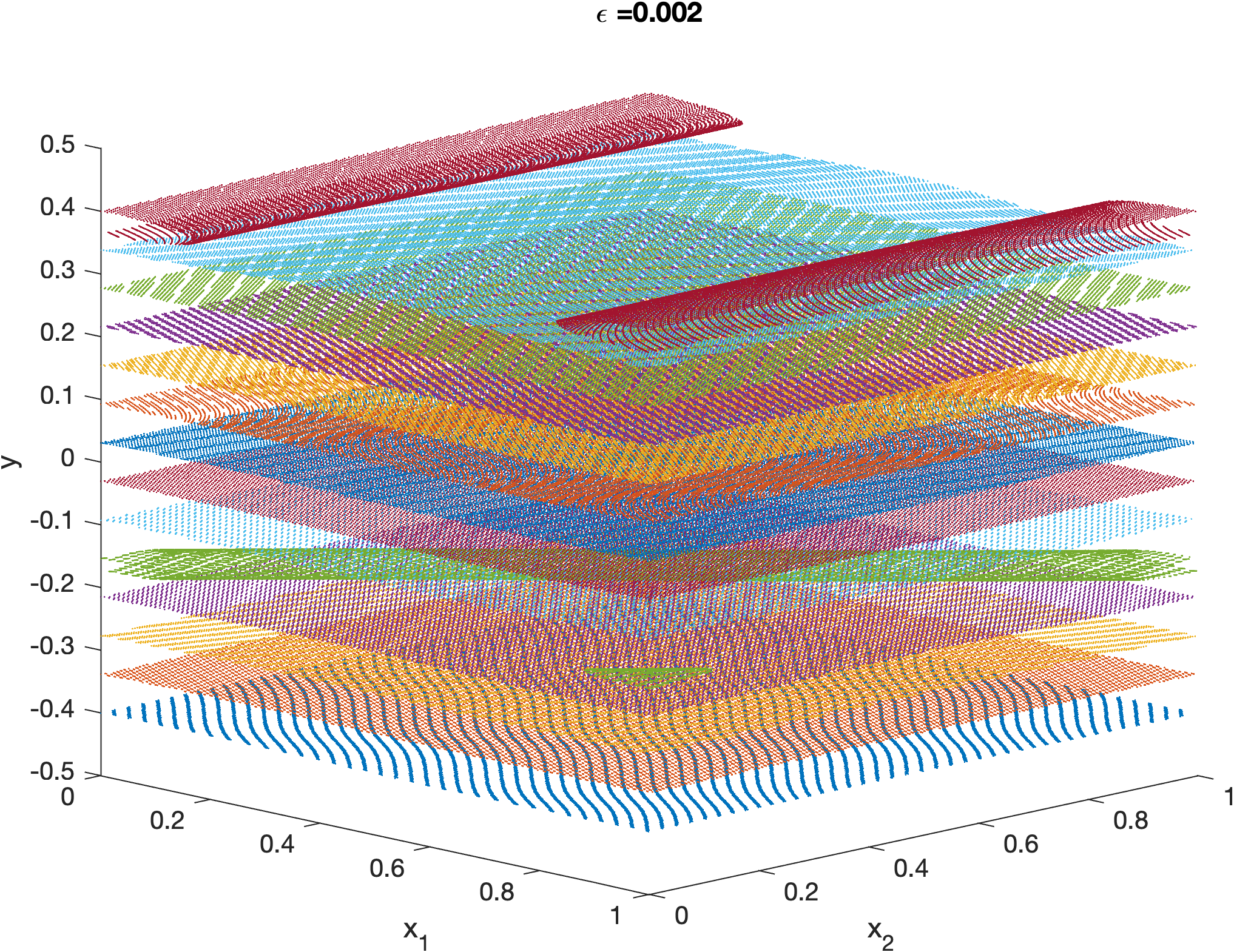
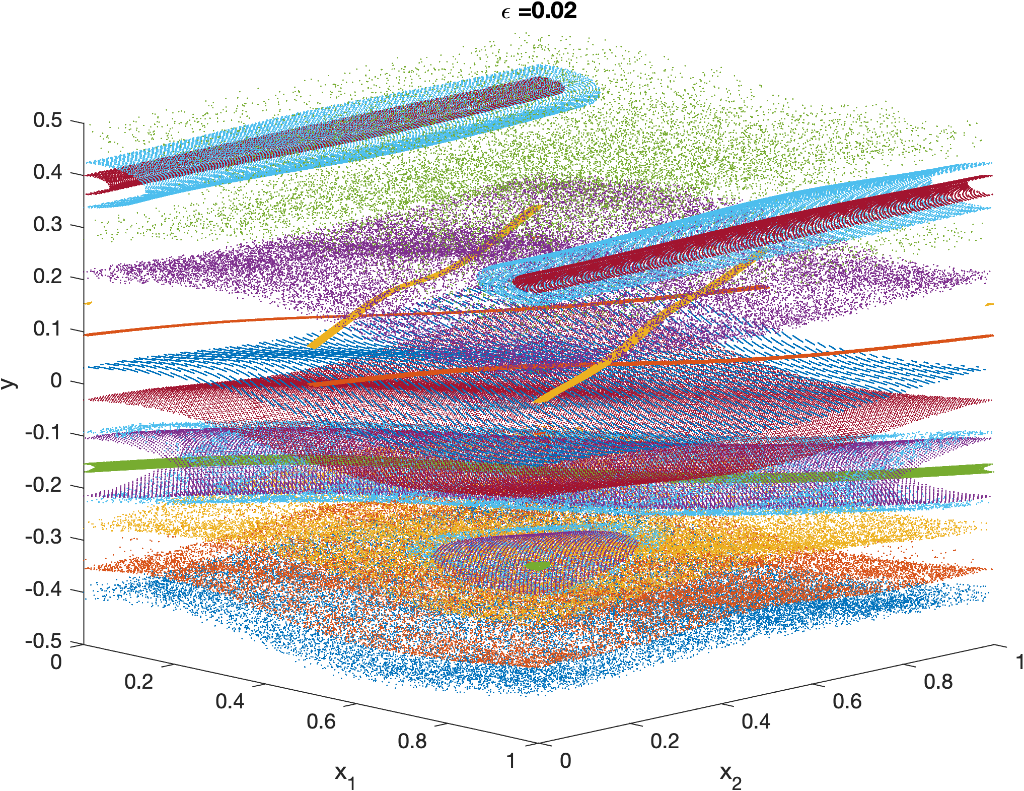
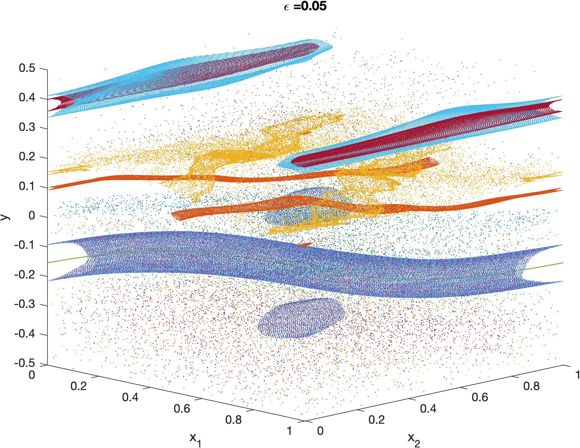
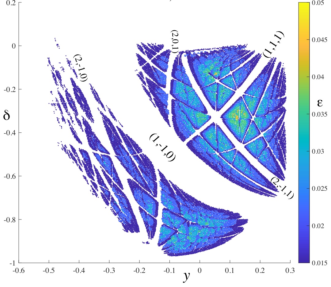
Figure 1: (a-c) Orbits for (1) and (6) for $\delta=-0.4$ and three values of $\varepsilon$. All initial conditions have $x_{1}=0,x_{2}=0$. Each image shows fourteen different orbits with $y_{0}\in[-0.4,0.5]$. As $\varepsilon$ increases, the number of rotational tori decreases, and at $\varepsilon=0.05$, only resonant tori and chaotic orbits are visible in the figure. (d) Values of $(y_{0},\delta)$ for which there are rotational tori with $\omega\in[0,1]^{2}$. The color represents the largest value of $\varepsilon$ with a corresponding rotational torus.

The first three panels of Fig. 1 show examples of orbits for (1) with (6) for three values of $\varepsilon$, and $\delta=-0.4$ (other values of $\delta$ exhibit similar behavior). As predicted by KAM theory, when $\varepsilon\ll 1$ the typical orbits appear to be dense on (rotational) two-tori ${\cal T}_{\omega}$ that are graphs over the angles $x$ with $y$ nearly constant. Even in Fig. 1(a), however one can see two resonant tubes. These are driven by the primary resonances, (5), of the force $F$, and correspond to the phases $x_{1}$ and $x_{1}-x_{2}$ remaining constant mod 1 (the third driven resonance, where $x_{2}$ is constant is out of range of the figure). These resonant tubes correspond to the resonances in Table 1 such that $(m,n)=(1,0,1)$ and $(1,-1,0)$ respectively. As $\varepsilon$ grows, more of the orbits become chaotic and other resonances become visible as tube-like structures, in particular the resonant tubes with $(m,n)=(2,-1,1)$ and $(2,1,2)$ seen in Fig. 1(b,c).

$(m,n)$	$y$	$(m,n)$	$y$
(1,1,1)	-0.481	(2,-1,0)	-0.317
(1,-1,0)	-0.164	(0,2,1)	-0.224
(1,1,1)	-0.019	(2,0,1)	-0.118
(1,0,1)	0.382	(2,-1,1)	0.090
		(2,1,2)	0.157
		(0,2,1)	0.224
		(1,2,2)	0.276
		(1,1,2)	0.494

Table 1: Action values for resonances up to order two in the range $|y|<0.5$ when $\varepsilon=0$ and $\delta=-0.4$.

We restrict our interest to tori with rotation vectors (3), in a fixed range, $\omega\in[0,1]\times[0,1]$. When $\varepsilon=0$, (6) implies that $\omega$ depends linearly on $\delta$ and quadratically on $y_{0}$. Indeed, each resonance in (16) defines a parabola (or a vertical line if $m_{2}=0$), $m\cdot\Omega(y_{0},\delta)=n$, in the $(y_{0},\delta)$ plane. When $\varepsilon$ is relatively small, we expect that persisting rotational tori will have rotation vectors that at least approximate this quadratic relationship. To illustrate this we compute the rotation vector $\omega$ using the methods described in §3 and §4 below. Fig. 1(d) shows the values of $(y_{0},\delta)$ for which there are rotational tori with $\omega\in[0,1]^{2}$. The color represents the largest $\varepsilon\in[0.015,0.045]$ for which a rotational torus exists for a given $(y_{0},\delta)$. The parabolic relationship between $y_{0}$ and $\delta$ is still clear in this image—the gaps represent initial conditions for which the corresponding orbits are resonant or chaotic. Several of the low order resonances are labeled in the figure. As $\varepsilon$ grows there are fewer initial conditions that lie on rotational tori, indicated by the dearth of yellow in Fig. 1(d).

Our primary goal is to study the persistence of rotational tori of (1) with conditions (6) as $\varepsilon$ grows from $0$. We observe in §4 that, for $\omega\in[0,1]^{2}$, there are rotational tori only when $\varepsilon<0.051$. In §5 we compute the most robust torus in subsets of this $\omega$ region; that is, the rotational torus with the largest maximum $\varepsilon$ value in the subset.

In our calculations, we use the $\varepsilon=0$ approximation to determine appropriate ranges for $y_{0}$ and $\delta$, setting $(y_{0},\delta)=\Omega^{-1}(p_{1},p_{2})$, i.e., inverting the frequency map (6), to obtain

$$(y_{0},\delta)\in{\cal P}=\{(p_{1}-\gamma,\beta(p_{1}-\gamma)^{2}-p_{2}):-0.05\leq p_{1},p_{2}\leq 1.05\}.$$ (8)

The added $0.05$ in ${\cal P}$ is a buffer to cover all $\omega\in[0,1]^{2}$ as $\varepsilon$ grows. Our calculations indicate this buffer is sufficient; indeed, we have checked that values of $(y_{0},\delta)$ outside this range do not give such $\omega$ values.

3 Weighted Birkhoff Averages

A finite-time Birkhoff average on an orbit of a map $f:M\to M$ beginning at a point $z\in M$ for any function $h:M\to{\mathbb{R}}$ is the sum

$$B_{T}(h)(z)=\frac{1}{T}\sum_{t=0}^{T-1}h\circ f^{t}(z).$$ (9)

This average need not converge rapidly. Even if the orbit lies on a smooth invariant torus with irrational rotation vector, the convergence rate of (9) is ${\cal O}(T^{-1})$, caused by edge effects for the finite orbit segment. By contrast, for the chaotic case, the convergence rate of (9) is observed to be ${\cal O}(T^{-1/2})$, in essence as implied by the central limit theorem [LM10].

The convergence of (9) on a quasiperiodic set can be significantly improved by using the method of weighted Birkhoff averages developed in [DSSY16, DDS⁺16, DSSY17]. Since the source of error in the calculation of a time average for a quasiperiodic set is due to the lack of smoothness at the ends of the orbit, we use a windowing method similar to the methods used in signal processing. Let

$$g(t)\equiv\left\{\begin{array}[]{ll}e^{-[t(1-t)]^{-1}}&t\in(0,1)\\ 0&t\leq 0\mbox{ or }t\geq 1\end{array}\right.\;,$$

be an exponential bump function that converges to zero with infinite smoothness at $0$ and $1$, i.e., $g^{(k)}(0)=g^{(k)}(1)=0$ for all $k\in{\mathbb{N}}$. To estimate the Birkhoff average of a function $h:M\to{\mathbb{R}}$ efficiently and accurately for a length $T$ segment of an orbit, we modify (9) to compute

$$\mathit{WB}_{T}(h)(z)=\sum_{t=0}^{T-1}w_{t,T}\,\,h\circ f^{t}(z)\;,$$ (10)

where

$$w_{t,T} =\frac{1}{S}g\left(\tfrac{t}{T}\right), S =\sum_{t=0}^{T-1}g\left(\tfrac{t}{T}\right)\;.$$ (11)

That is, the weights $w$ are chosen to be normalized and evenly spaced values along the curve $g(t)$. For a quasiperiodic orbit, the infinitely smooth convergence of $g$ to zero at the edges of the definition interval preserves the smoothness of the original orbit. Indeed it was shown in [DY18] that for a $C^{\infty}$ map $f$, a quasiperiodic orbit $\{f^{t}(z)\}$ with Diophantine rotation number, and a $C^{\infty}$ function $h$, it follows that (10) is super-convergent: there are constants $c_{n}$, such that for all $n\in{\mathbb{N}}$

$$\left|\mathit{WB}_{T}(h)(z)-\lim_{N\to\infty}B_{N}(h)(z)\right|<c_{n}T^{-n}.$$ (12)

Several papers [GMS10, LFC92, LV14] include a similar method to compute frequencies with a $\sin^{2}(\pi s)$ function instead of a bump function, but this function is fourth order smooth rather than infinitely smooth at the two ends, implying that the method converges as ${\cal O}(T^{-4})$, see e.g., [DSSY17, Fig. 7]. In addition to converging more rapidly, the weighted Birkhoff average (10) is relatively straightforward to implement.

4 Computing Tori

Using the weighted Birkhoff average (10), we can compute an approximation to a rotation vector $\omega$ as $\mathit{WB}_{T}(\Omega)$ for the frequency map (6). To discern whether an orbit lies on a rotational torus $T_{\omega}$ we must first distinguish chaotic from regular orbits, and then distinguish resonances from nonresonant tori.

By contrast to the case of regular orbits, when an orbit is chaotic (i.e., has positive Lyapunov exponents), (10) typically converges much more slowly; in general it converges no more rapidly than the unweighted average of a random signal, i.e., with an error ${\cal O}(T^{-1/2})$ [LM10, DSSY17]. We see in §4.1 that this distinction is valid for the map (1) as well.

Given a regular orbit, in §4.2, we use resulting the high-precision computation $\omega\simeq\mathit{WB}_{T}(\Omega)$ to define an approximate resonance order. This allows a distinction, up to some precision, between those orbits that have a commensurate frequency vector and those that appear to be nonresonant.

4.1 Distinguishing Chaos

To establish the distinction between chaotic and regular orbits, we estimate the number of digits of accuracy in the weighted Birkhoff average. Following [SM20], we compute (10) for two segments of an orbit, using iterates $\{1,\dots,T\}$ and $\{T+1,\dots,2T\}$; these values should be approximately equal when $T$ is large since the Birkhoff average depends only on the choice of orbit. A comparison of these gives the error estimate

$$dig^{(T)}_{h}=-\log_{10}\left|\mathit{WB}_{T}(h)(z)-\mathit{WB}_{T}(h)(f^{T}(z))\right|,$$ (13)

i.e., the number of consistent digits beyond the decimal point for the two approximations of $\mathit{WB}(h)$. If, for a modest value of $T$, $dig^{(T)}_{h}$ is relatively large, then the convergence is relatively rapid, meaning the orbit is regular. On the other hand, if $dig^{(T)}_{h}$ is small, then convergence is slow, with the implication that the orbit is chaotic.

Using $h=\Omega$, (6), the accuracy of the calculation of both components of $\omega$ is

$${dig^{(T)}}=\min\{dig^{(T)}_{\Omega_{1}},dig^{(T)}_{\Omega_{2}}\},$$ (14)

In addition to distinguishing chaotic and regular orbits, ${dig^{(T)}}$ can be used to estimate the precision of $\omega$. We will use these precision estimates in §5 when we consider number theoretic properties of the frequencies of the robust tori.

Fig. 2 shows the behavior of orbits when $\delta=-0.4$ and $\varepsilon=0.02$ for a set of initial conditions along the line $x_{1}=x_{2}=0$. Panel (a) is the slice with $|x_{2}|\leq 0.005$ through Fig. 1(b); it clearly shows a strongly chaotic region for $y\lesssim-0.41$, then narrower chaotic bands for $-0.41\lesssim y\lesssim-0.07$, followed by a region of tori and resonances up to $y\approx 0.27$, and finally a mixed regular/chaotic region up to $y=0.5$. The largest resonant regions shown correspond to $m=(1,-1)$ near $y=-0.16$, and $m=(1,0)$ near $y=0.38$; we also saw these in Fig. 1 and Table 1.

Fig. 2(b) shows corresponding values of ${dig^{(T)}}$ for three values of $T$. Even when $T=10^{3}$ (blue points), the calculations can distinguish between strongly chaotic—where ${dig^{(T)}}\sim 2-4$—and regular orbits—where ${dig^{(T)}}\sim 8$. However there is a population of orbits, especially those near the edges of resonant regions, that have intermediate values of ${dig^{(T)}}$, and for these it is harder to obtain a definitive classification. When $T=3(10)^{4}$ (orange points), the values of ${dig^{(T)}}$ become better separated—with regular orbits having ${dig^{(T)}}\sim 13-14$ and chaotic orbits still having ${dig^{(T)}}\sim 2-4$ —but there are still a fair number of intermediate values, again especially at the region edges. However, when $T=10^{6}$ (red points), regular orbits predominantly achieve full floating point accuracy, ${dig^{(T)}}\sim 14-16$, while chaotic orbits still have ${dig^{(T)}}\lesssim 5$.

Fig. 2(c) shows the components of $\omega$ computed for $T=10^{6}$. Each of the flat intervals corresponds to a range of $y$ values in a resonant tube, and these are bounded by chaotic regions where the computed values of $\omega$ vary rapidly with $y$ and the corresponding accuracy is low.

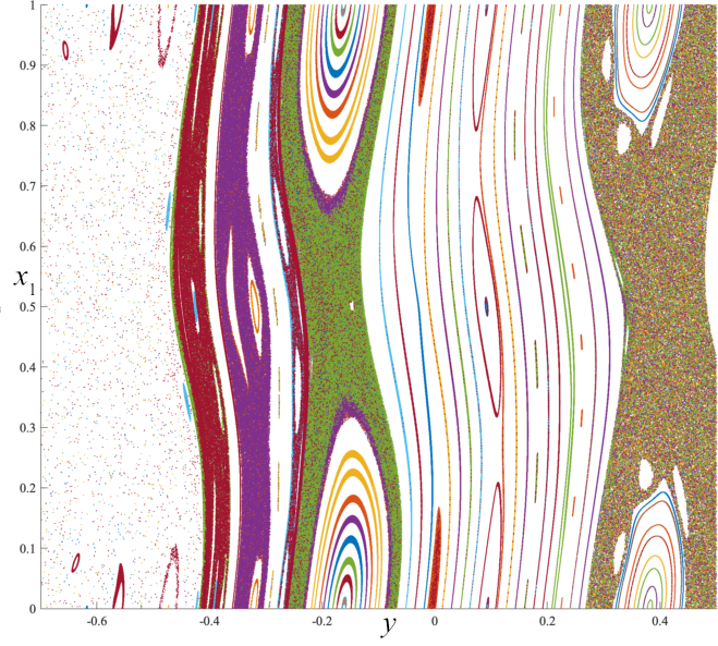
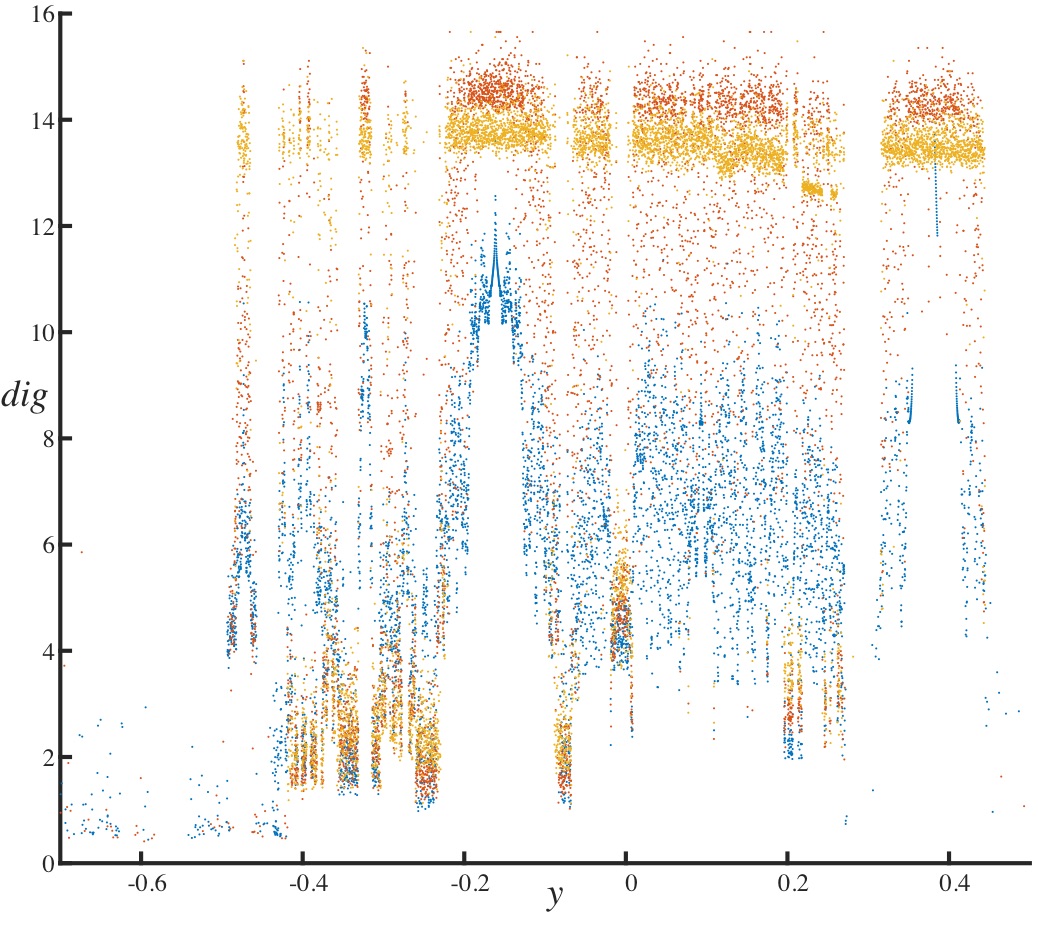
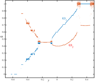
Figure 2: Orbits of (1) for $\delta=-0.4$, and $\varepsilon=0.02$ with initial conditions $(0,0,y)$ and a grid of $10^{4}$ initial $y$ values between $-0.7$ and $0.5$ (a) Slice for $|x_{2}|\leq 0.005$ showing the $(y,x_{1})$ phase space. (b) ${dig^{(T)}}$, (14), as a function of initial $y$ for $T=10^{3}$ (blue), $3(10)^{4}$ (orange), $10^{6}$ (red). The value of ${dig^{(T)}}$ changes significantly more at the edge of resonant tubes than it does in the middle of the tube, and for small $T$ the accuracy of the computation is low. (c) The two components of the rotation vector $\omega$ using $T=10^{6}$.

The dichotomy between the values of ${dig^{(T)}}$ for chaotic and regular orbits is also reflected in histograms of ${dig^{(T)}}$, shown in Fig. 3. These show the fraction of those orbits with $\omega\in[0,1]^{2}$ that have a given value of ${dig^{(T)}}$ for a range of $\delta$, $\varepsilon$, and initial conditions $(0,0,y_{0})$, with $y_{0}$ and $\delta$ chosen such that $(y_{0},\delta)\in{\cal P}$, (8). For the smaller $T$, panel (a), there are clear peaks near ${dig^{(T)}}=2$ and $14$ corresponding to chaotic and regular orbits, respectively, but there is also a broad shoulder with $8<{dig^{(T)}}<13$ that corresponds to orbits for which the distinction is less clear. Note, however, that in panel (b), where $T=10^{6}$, this middle peak has moved to larger values of ${dig^{(T)}}$, leaving only a smaller tail just below the peak at ${dig^{(T)}}=14$.

           

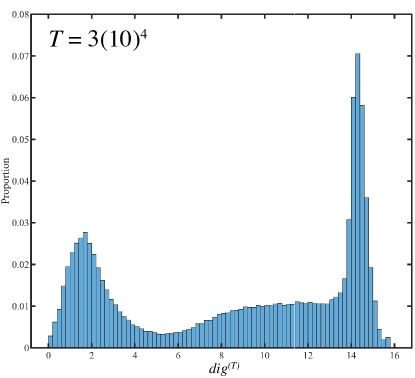
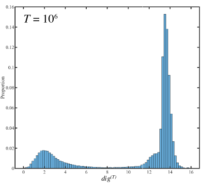
Figure 3: Frequency histograms of ${dig^{(T)}}$ for (a) $T=3(10)^{4}$ and (b) $T=10^{6}$ for a $100\times 100$ grid on the domain ${\cal P}$, (8), for initial conditions ($0,0,y_{0})$ and 50 values of $\varepsilon\in[0.005,0.055]$.

As we saw in Fig. 1, as $\varepsilon$ increases the chaotic region expands. Many of the chaotic orbits leave the interval $-0.7<y<0.5$; as a consequence, the computed frequencies for these orbits will be outside $[0,1]^{2}$. We think of the orbits that leave the $\omega$ range as essentially unbounded, though we cannot guarantee that there are no rotational tori acting as barriers at larger or smaller action values. Fig. 4(a) shows the proportion of the $10^{4}$ orbits in Fig. 3 that are bounded as $\varepsilon$ grows. Since ${\cal P}$ includes a buffer, at $\varepsilon=0$, the proportion is $1/1.1\approx 91\%$, but by the time $\varepsilon=0.055$, that proportion has dropped to about 10%. Only the bounded orbits were used in the histograms in Fig. 3.

Figure 4(b) shows for bounded orbits how the proportions of values of ${dig^{(T)}}$ that are small, intermediate, and large vary with respect to $T$. As $T$ grows, the fraction of orbits in the intermediate range, ${dig^{(T)}}\in(5,11)$, decreases, and the corresponding fractions in the lower and upper ranges saturate. In order to choose a measure to provide a good separation between order and chaos, we set $T=10^{6}$ for subsequent computations.

           

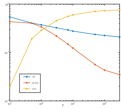
Figure 4: (a) The proportion of orbits in ${\cal P}$ with $\omega\in[0,1]^{2}$ as a function of $\varepsilon$. As the tori are destroyed, only a small fraction of orbits have computed rotation vectors in this range. (b) Log-log plot of the proportion of bounded orbits with ${dig^{(T)}}$ $<5$ (blue), between $5$ and $11$ (red), and $>11$ (yellow) as a function of $T$.

Fixing $T=10^{6}$, we next need to choose an appropriate cutoff value for $dig^{(10^{6})}$ to distinguish order from chaos. Fig. 5 shows the proportion of orbits with $dig^{(10^{6})}<7,9,11$. Even though varying the cutoff does give quantitative differences, the proportions have the same qualitative form as $\varepsilon$ varies. In particular, the proportions grow when $\varepsilon<0.03$, reflecting the increasing fraction of bounded orbits that are chaotic. Beyond the peak at $\varepsilon=0.03$, the fraction of unbounded orbits increases rapidly as the tori, which act as transport barriers, are destroyed, allowing the escape of previously trapped, chaotic orbits. Since we want to be conservative in classifying an orbit as a regular—as well as to guarantee that $\omega$ has high accuracy—we use the cutoff

$$dig^{(10^{6})}>11$$ (15)

to declare that an orbit is “nonchaotic.”

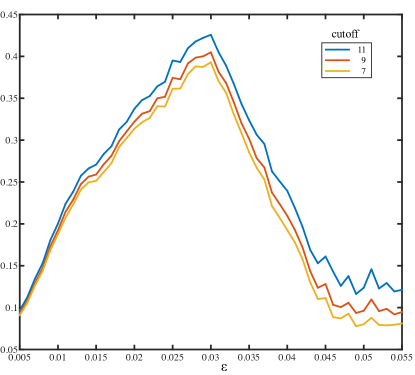
Figure 5: The proportion of orbits that would labeled as “chaotic” in ${\cal P}$ with $\omega\in[0,1]^{2}$ using the criteria ${dig^{(T)}}<7,9,11$ respectively with $T=10^{6}$. In each case the proportion peaks near $\varepsilon=0.03$. By criterion (15), the blue (11) curve shows the proportion of chaotic orbits.

Fig. 6 shows the set of frequencies for the nonchaotic, bounded orbits as a function of $\varepsilon$ as identified using the criterion (15). Note that this number drops significantly for large values of $\varepsilon$.

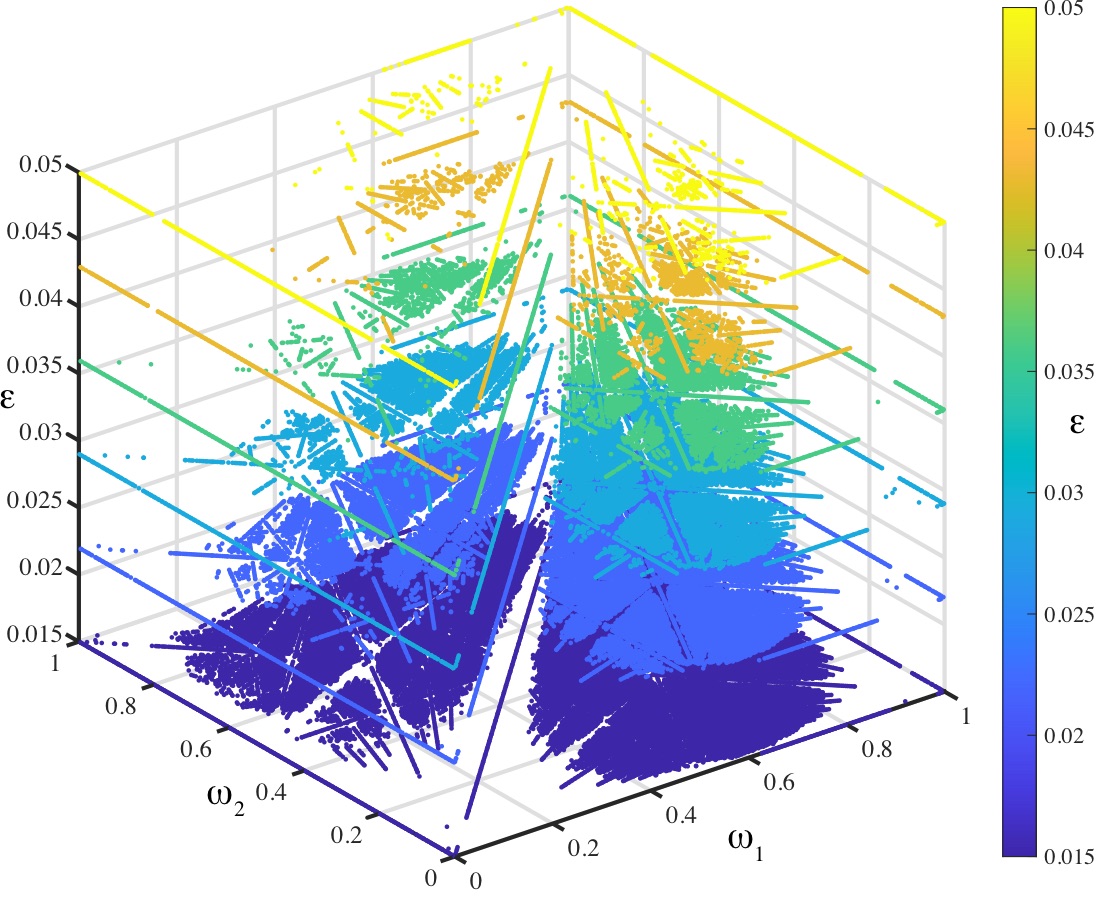
Figure 6: Rotation vectors $\omega\in[0,1]^{2}$ for the $1,613,136$ nonchaotic, bounded orbits, computed using a $1000^{2}$ grid in the domain ${\cal P}$, (8), and $\varepsilon\in[0.015,0.022,0.029,0.036,0.43,0.05]$, determined using the criteria in (15). As we see in §4.2, the straight lines correspond to orbits trapped in low-order resonant tubes.

4.2 Distinguishing Resonances

In this section, we seek a numerical method to distinguish between resonant and incommensurate vectors. For a given $\omega\in{\mathbb{R}}^{d}$, define the resonant module

$${\cal L}(\omega)\equiv\{m\in{\mathbb{Z}}^{d}:m\cdot\omega\in{\mathbb{Z}}\}.$$ (16)

We say that $\omega$ is incommensurate when ${\cal L}(\omega)=\{0\}$. By contrast, $\omega$, is resonant if (16) is nontrivial, i.e., if there is a nonzero vector $m\in{\mathbb{Z}}^{d}$ that satisfies (5). Of course, if $m,m^{\prime}\in{\cal L}(\omega)$, then so are $m+m^{\prime}$ and $km$ for any $k\in{\mathbb{Z}}$: the set (16) of such vectors is a module. The length, $M=\|m\|_{1}$, of the smallest (nonzero) integer vector $m$ in ${\cal L}(\omega)$ is the order of the resonance.

The rank of a resonant frequency $\omega$ is the dimension of ${\cal L}(\omega)$. We say that a frequency is rational if $\dim({\cal L}(\omega))=d$. In this case there is a $(p,q)\in{\mathbb{Z}}^{d+1}$ so that $\omega=\frac{p}{q}$; i.e., $\omega\in{\mathbb{Q}}^{d}$. When $d>1$, every rational frequency is resonant, but the converse need not be not true. For example, the vector $(\sqrt{2},2+3\sqrt{2})$ is resonant with $(m,n)=(-3,1,2)$, but it is not rational. For this example the resonance order is $M=4$.

Since we can compute the frequency vector for an orbit only to finite precision, we can only evaluate resonance up to some precision. If $\omega\in{\mathbb{R}}^{d}$ is $(m,n)$ resonant, then it lies in the codimension-one plane

$${\cal R}_{m,n}=\{\alpha\in{\mathbb{R}}^{d}:m\cdot\alpha-n=0\}.$$ (17)

The collection of resonant vectors is

$${\cal R}=\bigcup_{m,n\in{\mathbb{Z}}^{d+1}\setminus\{0\}}{\cal R}_{m,n}.$$ (18)

For the case $d=2$ of interest here, the lines up to order $M=8$ are shown for a portion of the $\omega$-plane in Fig. 7. Of course ${\cal R}$ is dense in ${\mathbb{R}}^{d}$, as are the Diophantine vectors (4).

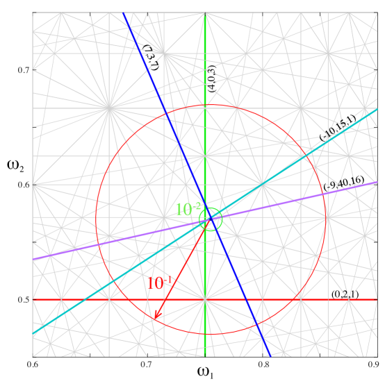
Figure 7: Resonant lines (grey), ${\cal R}_{m,n}$, up to order $M=8$. Also shown are those of minimal order for the spiral mean frequency $(\sigma^{-1},\sigma^{-2})$, see (22), for five values of $\rho$, $10^{-1}$ to $10^{-5}$ from Table 2.

We will say a vector $\omega$ is $(m,n)$ resonant to precision $\rho$ if the resonant plane intersects a ball of radius $\rho$ about $\omega$, i.e., if

$${\cal R}_{m,n}\cap B_{\rho}(\omega)\neq\emptyset.$$ (19)

Using the Euclidean norm, the minimum distance between the resonant plane and the point $\omega$ is

$$\Delta_{m,n}(\omega)=\min_{\alpha\in{\cal R}_{m.n}}\|\alpha-\omega\|_{2}=\frac{|m\cdot\omega-n|}{\|m\|_{2}}.$$ (20)

Thus we say that $\omega$ is $(m,n)$ resonant to precision $\rho$, whenever $\Delta_{m,n}(\omega)\leq\rho$.

Given a vector $\omega$ and a precision $\rho$, what is the smallest order resonance with $\Delta_{m,n}(\omega)\leq\rho$? For the one-dimensional case ($d=1$), the answer to this question can be efficiently computed using the Stern-Brocot (or Farey) tree. Indeed, as we previously noted [SM20], for any $\rho>0$, the rational $\tfrac{p}{q}$ with the smallest denominator in the interval $[\omega-\rho,\omega+\rho]$ is the first such rational on the tree that falls in that interval. The Stern-Brocot tree is essentially the generalization of the continued fraction to include “intermediates” as well as convergents of $\omega$.

As far as we know, there is no generalization of this result for $d>1$. Since there are finitely many $m\in{\mathbb{Z}}$ with $\|m\|_{1}\leq M$, a brute force computation is of course possible for modest values of $M$. For example, given any $\rho>0$, and ignoring issues of floating point arithmetic, Algorithm 1 will return

$$M(\omega,\rho)=\min\{\|m\|_{1}:\Delta_{m,n}(\omega)\leq\rho\},$$ (21)

which we could call $\rho$-order of $\omega$.

Algorithm 1 Minimal resonance order (21) to precision $\rho$ for $\omega\in{\mathbb{R}}^{d}$.

procedure ResonanceOrder($\omega$,$\rho$)

     $M=0$, $\Delta=1$

     while $\Delta>\rho$ do

         $M\leftarrow M+1$

         for $m_{2}=-M$ to $M$ do

              $m_{1}=M-|m_{2}|$

              $n=\mbox{round}(m\cdot\omega)$

              $\Delta=\min\left(\Delta,\frac{|m\cdot\omega-n|}{\|m\|_{2}}\right)$

         end for

     end while

return $M$

end procedure

As an example, consider the so-called spiral [KO86] or plastic [Ste96] mean, the real solution to

$$\sigma^{3}=\sigma+1\Rightarrow\sigma\approx 1.324717957244746.$$ (22)

This generates an algebraic field ${\mathbb{Q}}[\tau]$ with integral basis $(1,\tau,\tau^{2})$. The sequence of minimal order resonances for the frequency $(\sigma^{-1},\sigma^{-2})=(\sigma^{2}-1,\sigma-\sigma^{2}+1)$ with tolerances $\rho=10^{-j}$ for $j$ up to $14$ is shown in Table 2. For example, $M(\omega,10^{-9})=1119$. Note that this vector is Diophantine (4) [Cus72]. The first five optimal resonant lines are shown in Fig. 7.

$\log_{10}(\rho)$	$\|m\|_{1}$	$m_{1}$	$m_{2}$	$n$
-1	2	0	2	1
-2	4	4	0	3
-3	10	7	3	7
-4	25	-10	15	1
-5	49	-9	40	16
-6	96	7	89	56
-7	208	171	-37	108
-8	387	316	71	279
-9	1119	-350	769	174
-10	2064	-176	1888	943
-11	4306	3952	354	3185
-12	10322	6783	3539	7137
-13	24301	10676	-13625	295
-14	48897	-10971	37926	13330

Table 2: Optimal resonances and resonance orders for the frequency $\omega=(\sigma^{-1},\sigma^{-2})$, seen in Fig. 7, as the precision $\rho$ decreases. Note that without loss of generality, we can assume that $n$ is nonnegative.

The resonance orders (21) in Table 2 grow as a power of the inverse of the precision $\rho$ with the best-fit

$$M(\omega,\rho)\simeq 0.944\,\rho^{-0.336}.$$

Here is the intuition as to why this occurs: by Th. 1 in App. A, for each $K>0$, there is an $m\in{\mathbb{Z}}^{2}$ with $\|m\|_{\infty}\leq K$ such that for $p=2$

$$\Delta_{m,n}\leq\frac{1}{\|m\|_{2}K^{p}}.$$ (23)

Furthermore, a result of Laurent, see e.g., [Wal12, p. 693], implies that for almost all $\omega\in{\mathbb{R}}^{2}$, it is not possible to satisfy this equation for any value of $p>2$. Therefore, we expect that the typical value of $\|m\|_{\infty}$ is close to the maximal value, i.e., that the satisfaction of this bound requires that $\|m\|_{\infty}\sim K$. Then since the norms of $m$ are equivalent, choosing $K=\rho^{-1/3}$, we get $\Delta_{m,n}\lesssim\rho$, for $\|m\|_{1}\sim\rho^{-1/3}$.

More generally, for a given $\rho$, we computed the minimal resonance order (21) for a set of equi-distributed, random $\omega\in[0,1]^{2}$, see Fig. 8(a). The log of these values have mean $\langle\log_{10}M(\omega,10^{-9})\rangle=2.92$ and standard deviation $0.171$, though the distribution differs significantly from a normal with the same mean and deviation (the red curve in the figure). For the $10^{4}$ randomly chosen $\omega$ we found that

$$M(\omega,10^{-9})\leq m_{max}=3841,$$ (24)

and only six cases had $M>2500$. A similar distribution holds for other values of $\rho$. As shown in Fig. 8(b), the mean of $\log(M)$ depends linearly on $\log(\rho)$, with the best fit

$$\langle\log_{10}M(\omega,\rho)\rangle=-0.334\log_{10}(\rho)-0.091,$$ (25)

which is again consistent with (23).

           

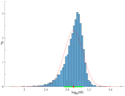
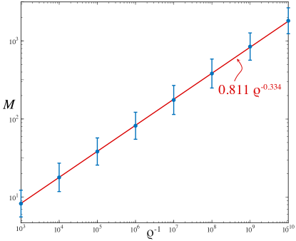
Figure 8: (a) Probability density of the logarithms of minimal resonance orders (21) for $10^{4}$ random vectors with precision $\rho=10^{-9}$. The dot (red) on the horizontal axis shows the mean, $2.92$, the thick line (green) shows one standard deviation $0.171$, and the curve (red) shows the normal distribution with these parameters. (b) A log-log plot of the mean and standard deviation of resonance order as a function of precision for a sample of $2000$ random vectors. The line (red) is the least squares fit (25).

The computation of the minimal resonance order is applied to the dynamical frequency vectors in Fig. 9 using $\rho=10^{-9}$. The data corresponds to the nonchaotic orbits on a grid of $(y,\delta)$ for $\varepsilon=0.043$. The orbits with $M<8$ (dark blue), clearly lie on the low-order resonant lines (grey) shown in the figure. Of the nonchaotic orbits at this value of $\varepsilon$, only $76$ have $M>250$, and only $79$ have $M>200$. It is clear that for this value of $\varepsilon$, there are very few rotational tori. A similar picture is obtained when more values of $\varepsilon$ are included in Fig. 10. The left panel shows the frequency vectors for the nonchaotic orbits of Fig. 6, now projected onto the $\omega$ plane. Note that many of the resonant lines lie in gaps in the figure, with clear clusters of points along the resonances. Indeed, if we change the color scale to be $\log_{10}M(\omega,\rho)$ for $\rho=10^{-9}$, the resonances again show up as dark blue lines, see Fig. 10(b).

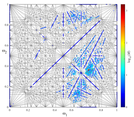
Figure 9: Frequencies of the $140,338$ nonchaotic orbits on a $1000^{2}$ grid in (8) of initial conditions for $\varepsilon=0.043$. The color scale is $\log_{10}(M)$. Only $76$ of these orbits have $\log_{10}(M)>2.4$. Also shown are the resonant lines, ${\cal R}_{m,n}$, up to order $8$.

           

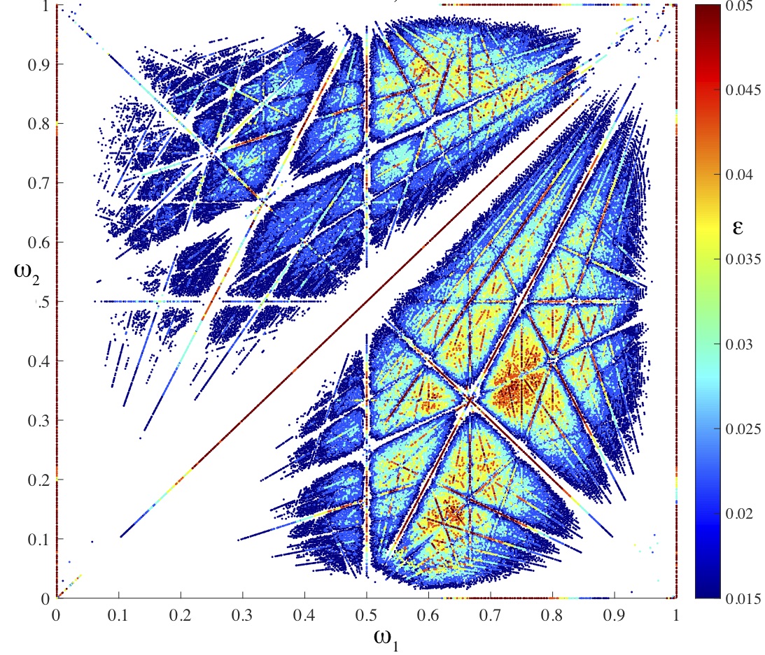
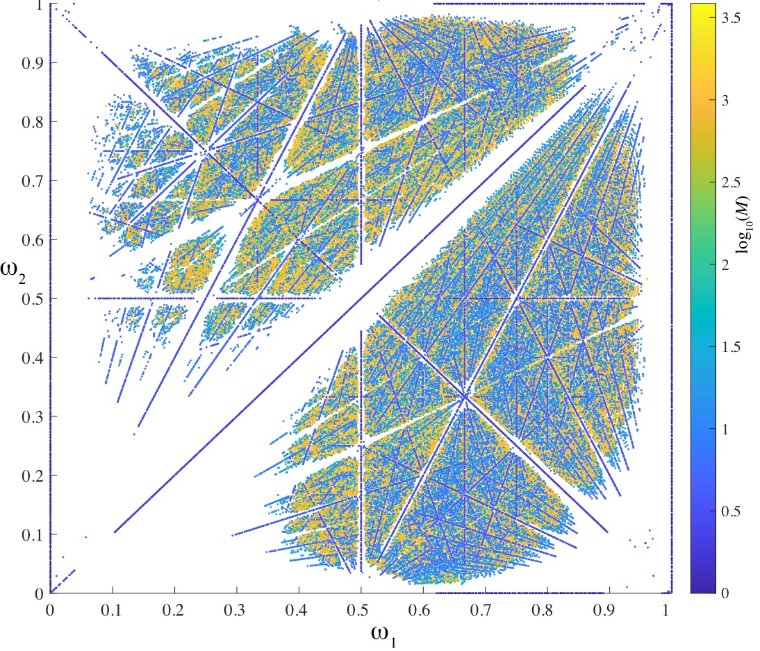
Figure 10: (a) The rotation vectors for nonchaotic orbits, using the same data of Fig. 6, now viewed in a two-dimensional projection. The color scale gives largest $\varepsilon$ for which there is a nonchaotic orbit for the given $(y_{0},\delta)$. (b) The same data, but this time colored using the $\rho$-order, (21).

Since randomly chosen $\omega$ will almost always be incommensurate, the dynamically obtained frequency vectors that are resonant should have values of (21) below the bulk of the distribution shown in Fig. 8. This is confirmed in Fig. 11(a), a histogram of resonance orders for the orbits from Fig. 6. Note how resonant tubes in the dynamics change the histogram from that of the random frequencies in Fig. 8. Indeed about $60\%$ of these orbits have $M=1$ or $2$ corresponding to the largest resonances due to the Fourier terms of the force (6), and only $20\%$ have $M>250$, i.e., the bulk of the domain of Fig. 8.

           

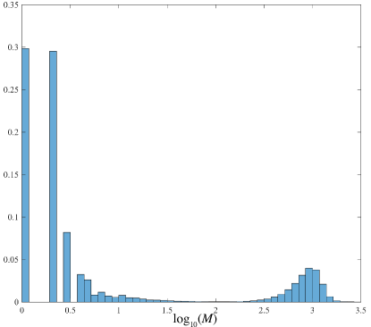
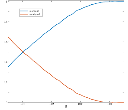
Figure 11: (a) Histogram of $\log_{10}(M)$ for the data of Fig. 6. (b) The fractions of nonchaotic orbits with $\omega\in[0,1]^{2}$ that correspond to resonant (blue) and rotational tori (red) as a function of $\varepsilon$.

For our calculations, we will declare $\omega$ to be resonant if $\log_{10}(M)$ is more than three standard deviations below the mean of the random data of Fig. 8. Given that the cutoff (15) gives at least $11$-digit accuracy in $\omega$, we will use $\rho=10^{-9}$ so that the computation of $\Delta_{m,n}<\rho$ from (20) has significance. In summary we use the cutoff

$$M(\omega,10^{-9})>10^{2.4}=251$$ (26)

to declare that an orbit “nonresonant”.

Now that we have introduced the full computational method, we give some information its computational complexity. The total runtime starting with initial conditions and distinguishing chaotic from nonchaotic and resonant from rotational orbits in Matlab 2020b using a 14-core Intel Xeon W processor at $2.5$ GHz with $64$ GB memory is approximately $2250$ orbits per minute. The computation of $M(\omega,10^{-9})$ for $2250$ frequency vectors takes approximately 32 seconds, i.e., roughly half the calculation time.

Applying this criterion to the data in Fig. 10, separates the $80\%$ of the orbits that are resonant, shown in Fig. 12(a), from the remaining $20\%$ of orbits that are not resonant, shown in Fig. 12(b). We assume that each of these latter orbits lies on a rotational torus, ${\cal T}_{\omega}$.

           

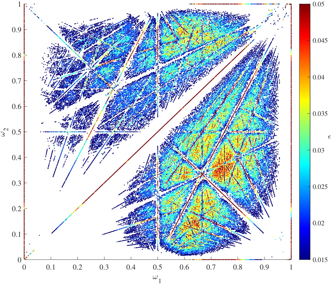
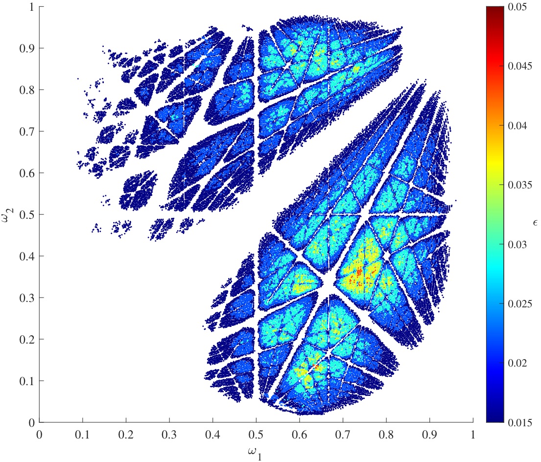
Figure 12: Frequency vectors for (a) $1,295,986$ resonant orbits and (b) $317,150$ nonresonant orbits, using the data of Fig. 6. These are distinguished by the criterion (26). Values are colored by the largest $\varepsilon$ for which a torus persists at the corresponding $(y_{0},\delta)\in{\cal P}$.

5 Critical Sets

In this section we investigate the robustness of invariant tori as a function of the perturbation strength $\varepsilon$. In particular we are interested in finding critical tori: those on the threshold of destruction. For smooth, two-dimensional, twist maps, an invariant circle with rotation number $\omega\in{\cal D}$ is critical if has a non-smooth conjugacy to the rigid rotation $\theta\mapsto\theta+\omega\mod 1$. This idea was extended to the three-dimensional case in [FM16]. Since we are not computing the conjugacy, we instead define $\varepsilon_{c}(\omega)$, following [MS92], to be a value at which a rotational torus ${\cal T}_{\omega}(\varepsilon_{c},y_{c},\delta_{c})$ breaks up; i.e., in any neighborhood $\mathcal{N}$ of $(y_{c},\delta_{c})$, there is a $\Delta\varepsilon>0$ such that when $\varepsilon_{c}<\varepsilon<\varepsilon_{c}+\Delta\varepsilon$, there is no torus ${\cal T}_{\omega}(\varepsilon,y,\delta)$ with the same rotation vector for any $y,\delta\in\mathcal{N}$.

When $\omega\in{\cal D}$, and $\Omega(y,\delta)$ is a bijection and satisfies a twist condition, then KAM theory implies that for small enough $\varepsilon>0$ a torus will exist for some point $(y_{0},\delta)$ [CS90, Xia92]. On the other hand, each resonant torus, ${\cal T}_{\omega}(0,y_{0},\delta)$ for $(y_{0},\delta)=\Omega^{-1}({\cal R})$, generically breaks up at $\varepsilon=0$. Define the critical set

$$\varepsilon_{c}(\omega)=\left\{\varepsilon:{\cal T}_{\omega}(\varepsilon,y_{0},\delta)\mbox{ breaks up for some }(y_{0},\delta)\in{\cal P}\right\}.$$ (27)

For the simplest, two-dimensional case, e.g., the one-parameter Chirikov standard map, the critical set appears to be a graph over $\omega$, and each invariant circle—once destroyed—does not reappear [MS91]. However critical set can be much more complicated for maps with several parameters, e.g., multiharmonic maps [BM94], or for nontwist maps [FWAM06]. For the standard volume-preserving map, (6), we do not actually know whether the critical set is simple, with only one breakup for each $\omega$. Nevertheless, we expect that $\varepsilon_{c}(\omega)=0$ whenever $\omega\in{\cal R}$ and $\varepsilon_{c}(\omega)>0$ for $\omega\in{\cal D}$. Since both of these sets are dense, the critical surface will be nowhere continuous.

5.1 Locally Robust Tori

As an illustration of the critical set, Fig. 13 shows tori that exist for a $100\times 100$ grid in ${\cal P}$, (8), for $50$ evenly spaced $\varepsilon\in[0.015,0.045]$. A point $(\omega,\varepsilon)$ is shown in the figure if the parameters $(\varepsilon,y_{0},\delta)$ give a rotational torus, ${\cal T}_{\omega}(\varepsilon,y_{0},\delta)$, using the criteria described in §4. The upper boundary of the points shown provides a rough approximation of the critical set (27). Of the critical tori, some have locally maximal values of $\varepsilon_{c}(\omega)$, i.e., there is a neighborhood for which all critical tori have smaller $\varepsilon_{c}$. We will call such tori locally robust.

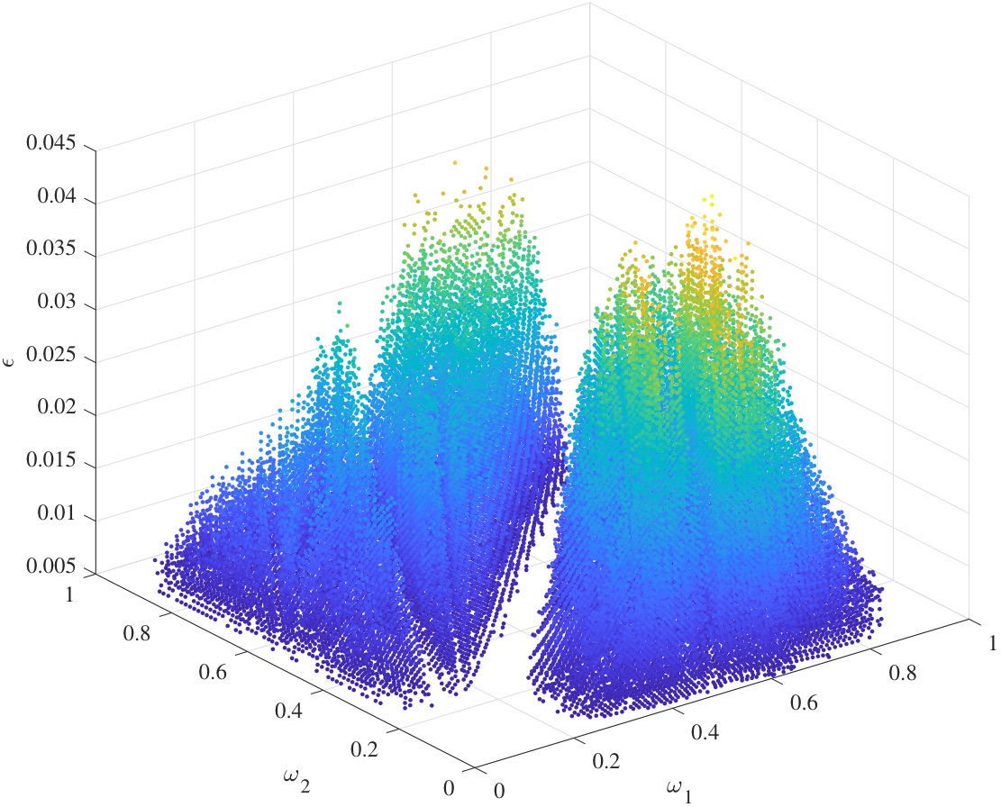
Figure 13: Rotation vectors corresponding to rotational tori, using a $100^{2}$ grid in the domain ${\cal P}$ (8), and 50 $\varepsilon$ values.

To find approximations for the locally robust tori in Fig. 13, we search for local peaks in sub-regions of the critical set using a refinement method that does not rely on smoothness. In particular, for a fixed subset of $[0,1]^{2}$, we start at $\varepsilon=0.01$ with a $100\times 100$ grid of corresponding points in $(y,\delta)$, keeping only those $(y,\delta)$ that correspond to a rotational torus in the $\omega$ region. At each step we refine the grid for the set of parameters that have tori and increment $\varepsilon\to\varepsilon+d\varepsilon$. Both the increment $d\varepsilon$ and the number of grid points are adapted depending on the tori at the previous $\varepsilon$. The grid size remains $100\times 100$ until the grid spacing is below $10^{-12}$ in the $y$ or the $\delta$ direction. After this point we use a $10\times 10$ grid. To choose the next $d\varepsilon$, if more than twelve tori remain at $\varepsilon$, then $d\varepsilon\to 1.3\cdot d\varepsilon$. If between four and twelve tori remain, $d\varepsilon$ is unchanged, and if fewer than four tori remain, $d\varepsilon\to d\varepsilon/2$. Finally, if no tori are found, then $d\varepsilon\to d\varepsilon/2$, and instead of increasing $\varepsilon$, we decrease it such that $\varepsilon\to\varepsilon-d\varepsilon$. Our procedure halts once we have determined a single value that is isolated on a grid of $10\times 10$ points such that $y_{\max}-y_{\min}$ and $\delta_{\max}-\delta_{\min}$ are both less than $10^{-12}$, and such that there is no torus in the same region for $\varepsilon+10^{-14}$. Thus these values should correspond to local peaks up to the corresponding accuracy in $\delta,y,\varepsilon$. Dividing $[0,1]^{2}$ into four regions, the maxima that we computed are listed in Table 3.

The global maximum, found in quadrant II where $\omega\in[\tfrac{1}{2},1]\times[0,\tfrac{1}{2}]$, agrees within $0.6\%$ for $\varepsilon$ and $\omega$ of the results in [FM13] that were achieved using Greene’s residue method. In that paper, tori were approximated using periodic orbits chosen on the Kim-Ostlund tree and the most robust torus was represented by a periodic orbit of period $32,316$. This torus was estimated to breakup at $\varepsilon=0.0512\pm 0.0005$. For the initial conditions corresponding to this value, the weighted Birkhoff method identifies the orbit as chaotic for $\varepsilon>0.0512-0.00050005$. Thus the identification of regular orbits using the Greene’s residue method in [FM13] is slightly less restrictive than the identification of regularity that we are using in the current paper.

Quadrant	I	II	III	IV
$\omega$-Region	$[0,\tfrac{1}{2}]^{2}$	$[\tfrac{1}{2},1]\times[0,\tfrac{1}{2}]$	$[0,\tfrac{1}{2}]\times[\tfrac{1}{2},1]$	$[\tfrac{1}{2},1]^{2}$
$\varepsilon$	0.031282089698381	0.051261692234977	0.032740058025373	0.041019021169048
$\delta$	-0.133386500670280	-0.334376117328629	-0.743481096516467	-0.884496372446711
$y$	-0.119301311749656	0.123097748168231	-0.162656510381853	-0.046691232395606
$\omega_{1}$	0.476213927381772	0.734410803700126	0.482238008029131	0.641541383714863
$\omega_{2}$	0.175290820661118	0.365412254352543	0.781945554897404	0.890319673258112

Table 3: Most robust tori in four $\omega$ regions. These were computed by successive refinement of a grid in ${\cal P}$.

We now give a more in depth computation of the critical set, taking slices through Fig. 13 by choosing a curve in $(y_{0},\delta)$-space. Such a slice, fixing $\delta$ and varying $y_{0}$, is shown in Fig. 14. Points here correspond to tori indicated in Fig. 1(d) along the horizontal line at $\delta=-0.4$. Here we plot the values of $\varepsilon$ for which there is a torus ${\cal T}_{\omega}(\varepsilon,y_{0},-0.4)$ as $y_{0}$ varies. The horizontal axis is taken to be $\omega_{1}$ since, when $\varepsilon=0$, $\omega_{1}=\Omega_{1}(y,-0.4)=y+\gamma$ is a bijection. Note that since the rotation vectors in Fig. 14 are computed on a fixed grid in $y_{0}$, they are not true peak values, like those we found by refinement in Table 3.

In this cross section, as well in similar cross sections for five other $\delta$ values, there appears to only be one critical torus at any $\omega$. In particular, the empty holes in the enlargement are sampling artifacts that go away when computing on a finer grid. As the enlargement shows, for each fixed $y_{0}$, the curve in $(\varepsilon,\omega_{1})$ begins as a line for small $\varepsilon$, but each bends as $\varepsilon$ grows, especially for those values approaching a visible resonant region. The curve for fixed $y_{0}$ does not always slope in the same direction, as we also will see below in Fig. 19. Gaps in these constant $y_{0}$ curves appear to be due to crossing such resonances. Unfortunately, since $\omega$ depends on $(y_{0},\delta,\varepsilon)$, the cross section is not a simple plane $\omega_{2}=$ constant. Nevertheless, since $\varepsilon$ is relatively small, the values of $\omega(y_{0},-0.4)$ lie almost on a curve, as shown in Fig. 14(b), that is close to the parabola in given by (8). This thickened curve has gaps due to resonances and has a maximum thickness $\Delta\omega_{2}\sim 0.001$. The thickness is largest when $0.5<\omega_{1}<0.9$ where, as is seen in Fig. 13(a), tori persist for larger $\varepsilon$.

Note that the critical set seen in Fig. 14(a) is visually similar to that for the standard map [MS92], which is zero on every rational and has local maxima on the noble numbers. In our case the zeros occur whenever the cross section intersects a resonant line, and the local maxima are perhaps narrower than in the 2D case.

           

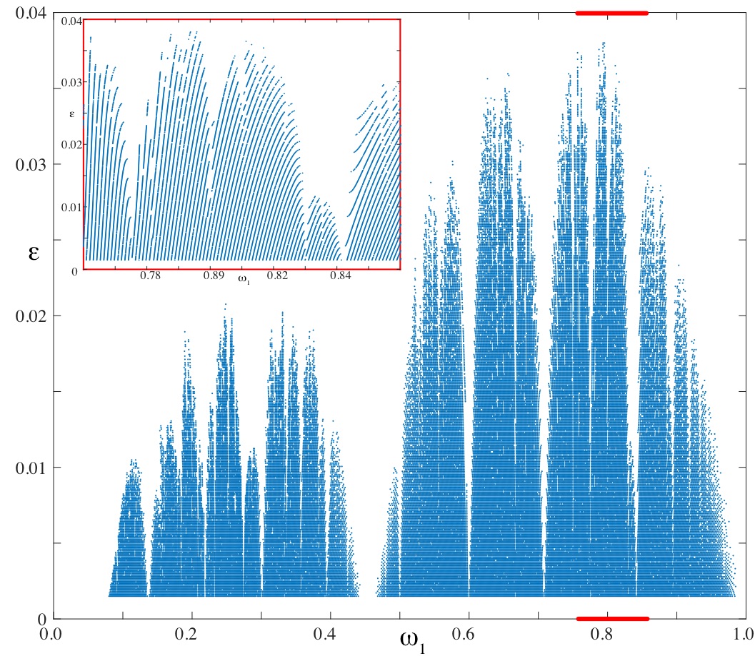
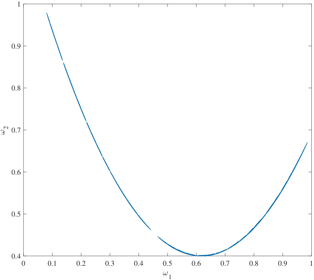
Figure 14: Rotation vectors for rotational tori with fixed $\delta=-0.4$ and for a grid of $1000$ $y\in[-0.05-\gamma,1.05-\gamma]$ as in (8) and a grid of $500$ $\varepsilon\in[0.0015,.055]$. (a) Data projected onto the $(\omega_{1},\varepsilon)$-plane, with an enlargement for a small $\omega_{1}$ range shown in the red box. (b) A projection of the same data onto the $\omega$-plane.

5.2 Best Approximants

Lochak [Loc92] conjectures that the robust two-tori for a symplectic map of the form (1) with $d=k=2$ will have rotation vectors such that $(\omega,1)$ is an integral basis for the cubic algebraic field of discriminant $49$ generated by

$$\alpha^{3}+\alpha^{2}-2\alpha-1\Rightarrow\alpha=2\cos(2\pi/7),$$ (28)

(see App. B). The field ${\mathbb{Q}}[\alpha]$ has an integral basis $(\omega,1)$ with

$$\omega=(\alpha^{2}-1,\alpha-1)\approx(0.554958132087371,0.246979603717467).$$ (29)

This field has the smallest discriminant amongst all totally real cubic fields. An alternative conjecture, probably due to Kim and Ostlund [KO86], is that the spiral field, (22), should give the generalization of the noble numbers for two-dimensional maps. The spiral mean is a Pisot (or PV) number: its minimal polynomial has only one root outside the unit circle [Cas57]. The spiral field is complex with discriminant $-23$, the smallest, in absolute value of all cubic fields; moreover, it is the smallest Pisot number (see App. B). We will consider the vector

$$\omega=(\sigma-1,\sigma^{-1})\approx(0.324717957244746,0.754877666246693),$$ (30)

which, together with $1$ gives an integral basis for ${\mathbb{Q}}[\sigma]$. Finally, [Tom96] considers the field with discriminant $-44$ and the minimal polynomial

$$\tau^{3}-\tau^{2}-\tau-1\Rightarrow\tau\approx 1.83928675521416,$$ (31)

and chooses a basis vector for ${\mathbb{Q}}[\tau]$ that is distinguished by having a repeated sequence in its Jacobi-Perron expansion (see App. B):

$$\omega=(\tau-1,\tau^{-1})=(0.83928675521416,0.543689012692076).$$ (32)

Here we would like to provide evidence for/against these conjectures.

As a first attempt, we investigate the Diophantine constants for the robust frequency vectors that we have found. As discussed in App. A the simultaneous Diophantine constant can be computed by finding rational approximations $\omega\approx\frac{p}{q}$, and computing ${\|{q\omega}\|_{\mathbb{Z}}}=\|q\omega-p\|_{\infty}$. The sequence of periods, $q_{i}$, (34), defined so that ${\|{q_{i}\omega}\|_{\mathbb{Z}}}$ decreases monotonically, corresponding to a sequence of best rational approximations $\omega\approx\frac{p_{i}}{q_{i}}$. A frequency vector is Diophantine if the sequence

$$c_{s}(\omega,q_{i})=q_{i}\|q_{i}\omega\|^{2}_{\mathbb{Z}}$$

is bounded away from zero as $q_{i}\to\infty$ (see (37)-(38) in App. A).

For example, the sequence of Diophantine constants $c_{s}(\omega,q_{i})$ for (29) are shown in Fig. 15(a) (see the data in Table 5 of App. A). These appear to oscillate quasiperiodically but are bounded below, giving an estimate $c_{s}(\omega)\approx 0.19$ for the $D=49$ field, at least for $q_{i}\leq 10^{8}$. It is conjectured that there is some integral basis in this field with Diophantine constant $\tfrac{2}{7}\approx 0.286$, and that this value is the largest possible for $d=2$ [Cus74]. The corresponding Diophantine sequence for (30) in the $D=-23$ field and (32) in the $D=-44$ field, are also shown in the figure—again they are bounded away from zero as is consistent with the known Diophantine property of cubic fields. The dependence of $c_{s}$ on $q_{i}$ is less regular for these two vectors than for the first case, and the limit infimum appears smaller, $c_{s}(\omega)\approx 0.1$.

We show in Fig. 15(b) the sequence of Diophantine constants computed for the four robust tori from Table 3. For these vectors, the values $c_{s}(\omega,q_{i})$ appear to be bounded away from zero for $q_{i}\lesssim 10^{5}$, but the values are smaller than the pure cubic vectors. Note however, that the peak in quadrant I could have $c_{s}(\omega)\simeq 0.1$, though numerical issues cause the value to drop when $q_{i}>10^{5}$.

           

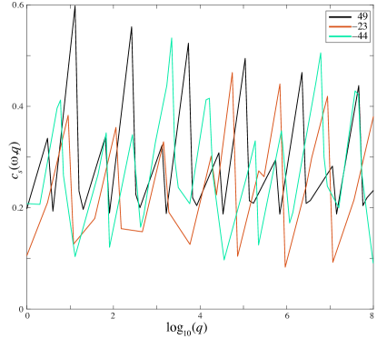
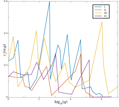
Figure 15: Diophantine constants for best approximants. (a) Frequencies in the cubic field with discriminants $D=49$ (29), $D=-23$ (30), and $D=-44$ (32). (b) The peak frequencies in the four quadrants of Table 3.

Figure 16 shows histograms of the Diophantine sequence $c_{s}(\omega,q_{i})$ for three different data sets. The first correspond to randomly chosen $\omega\in[0,1]^{2}$. Note that this distribution decreases monotonically, perhaps consistent with the expectation that there will be near rational vectors in a random collection. To construct a second data set, we fix the vector $(\alpha,\alpha^{2},1)$, an integral basis for the $D=49$ cubic field. Multiplication of this vector by any matrix $A\in SL(3,{\mathbb{Z}})$ results in another integral basis. We choose four elementary matrices that generate this group, and randomly draw a product of $50$ of these matrices to give a set of integral bases for this field. The resulting Diophantine constants have the distribution as shown in Fig. 16(b). Note that this distribution is peaked away from $c_{s}=0$.

Finally, in Fig. 16(c), we compute $c_{s}(\omega,q_{i})$ for the local peak data that is obtained as follows. A discrete approximation to $\varepsilon_{c}(\omega)$ is obtained from a $300\times 300$ grid in ${\cal P}$ and $50$ values of $\varepsilon\in[0.005,0.045]$ –a refinement of data set shown in Fig. 13. Then for each bin in $\omega$ of size $0.01$ ($100^{2}$ bins) we select $\varepsilon_{c}$ to be the largest of the $\varepsilon$ for tori with $\omega$ falling in that bin. This gives $3066$ bins that have tori with $\varepsilon_{c}>0.02$. Since the true critical surface is not smooth or continuous, these values almost certainly do not include the true local maxima for all $\omega$ in each bin; indeed the largest $\varepsilon_{c}$ on this grid in ${\cal P}$ is $0.045$, below that of the most robust torus in Table 3 that we found by refinement. Nevertheless, this process gives a set of tori that are more robust than their computed neighbors, so that these tori are, at least, locally robust, if not true local maxima.

Note that the maximum of the distribution for the peak tori is shifted to $c_{s}\sim 0.1$, considerably above that of the cubic field, indicating that the peak tori are preferentially selected to have larger Diophantine constants. Indeed, even though all three distributions have similar means and standard deviations, they are statistically different: a Kolmogorov-Smirnov test applied to these data sets indicates that these distributions are distinct with $p$-values that are extremely small.

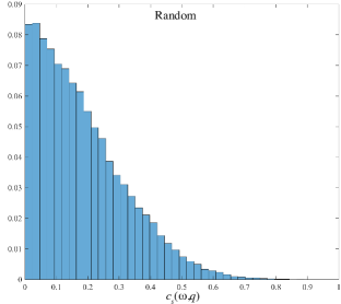
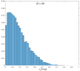
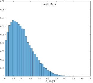
Figure 16: Histograms of Diophantine constants $c_{s}(\omega,q_{i})$ for the sequence of best periods $\{q_{i}\}$ for frequency vectors $\omega$ computed to $\|q_{i}\omega\|_{\mathbb{Z}}\leq\rho=10^{-11}$. (a) $4000$ random frequency vectors chosen from a uniform distribution in $[0,1]^{2}$ (mean $=0.180$, $\sigma=0.139$). (b) $4000$ vectors that are integral bases in the cubic field with discriminant $D=49$ (mean $=0.186$, $\sigma=0.135$) (c) $3066$ frequencies of tori that are locally robust on a $100^{2}$ grid for $\varepsilon>0.02$ (mean $=0.199$, $\sigma=0.134$).

The histograms shown Fig. 16 do not distinguish values of $c_{s}$ as a function of the period $q_{i}$. To do this, Fig. 17 shows two-dimensional histograms with bins for both $c_{s}$ and $\log_{10}(q)$. The comparison of the randomly generated data, in the left pane, with the data from the computed peak rotation vectors in the right pane, shows again the that the latter has significantly more values of $c_{s}$ bounded away from zero.

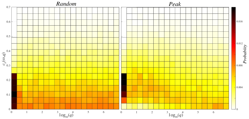
Figure 17: Diophantine constants vs $\log_{10}(q)$ for randomly chosen $\omega$ equi-distributed in $[0,1]^{2}$ (left panel) and “peak” tori of the volume-preserving map (right panel).

In conclusion, our compuations give strong evidence that the more robust tori preferentially have larger values of the simultaneous Diophantine constant, at least up to periods $q_{i}\sim 10^{6}$.

6 Continuation

In order to further test the conjectures on which classes of frequency vectors correspond to most robust tori, we study here the breakup of tori ${\cal T}_{\omega}$ for several fixed rotation vectors. In particular we will find tori for vectors in the three cubic fields that have the smallest discriminants: $D=-23$, $49$, and $-44$, recall (22), (28) and (31).

As we noted, each of these fields has properties making it a candidate to generalize of the set of noble numbers, ${\mathbb{Q}}[\phi]$. The field ${\mathbb{Q}}[\sigma]$ is generated by the smallest Pisot number and has bases that are periodic sequences in the Kim-Ostlund generalization of the Farey tree. The field ${\mathbb{Q}}[\alpha]$ is conjectured to have bases with the largest possible simultaneous Diophantine constant. The field ${\mathbb{Q}}[\tau]$ contains a basis with a period-one Jacobi-Perron sequence, one generalization of the continued fraction, see App. B.

For each case (29), (30), and (32), give vectors for which $(\omega,1)$ is an integral basis for the respective cubic field. Additionally, we will consider the permuted vector $(\omega_{2},\omega_{1},1)$, which gives an additional integral basis for the same field, so that there is a set of six vectors, $\omega^{*}$, that we study.

For each frequency vector, we continue the torus with respect to the parameter $\varepsilon$, e.g., finding ${\cal T}_{\omega^{*}}(\varepsilon,y(\varepsilon),\delta(\varepsilon))$, fixing $\omega=\omega^{*}$. We find the maximum $\varepsilon$ such that the corresponding torus is nonchaotic— using the ${dig^{(T)}}$ criterion (15). The torus is found using a predictor-corrector method starting with the guess $(y,\delta)=\Omega^{-1}(\omega^{*})$ at a small value of $\varepsilon$. Specifically, at each $\varepsilon$, we apply the Matlab root finder fsolve to find the value of $(\delta(\varepsilon),y(\varepsilon))$ such that the rotation vector is $\omega^{*}$ when computed using $\mathit{WB}_{10^{6}}$. We look for $\varepsilon_{c}$ such that ${dig^{(T)}}>11$, but for which ${dig^{(T)}}<11$ when $\varepsilon_{c}<\varepsilon<\varepsilon_{c}+10^{-9}$. Fig. 18 shows an example of the computation for (32). The results for other $\omega$ values appears quite similar. In particular, as seen in Fig. 18(b), ${dig^{(T)}}$ drops very quickly near the critical value.

           

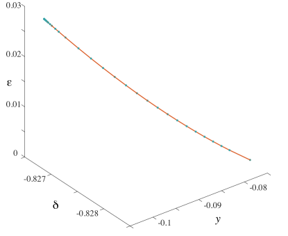
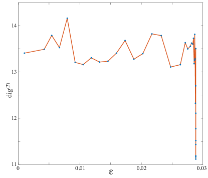
Figure 18: An example of a rotational torus found using a predictor-corrector continuation method using the weighted Birkhoff method. (a) The graph $(y(\varepsilon),\delta(\varepsilon))$ for a torus ${\cal T}_{\omega}(\varepsilon,y,\delta)$ with $\omega=(\tau^{-1},\tau-1)$ in the $D=-44$ field. (b) Number of correct digits in $\omega$ as a function of $\varepsilon$. This number drops precipitously as $\varepsilon$ approaches the critical value $0.028845453269968$, see Table 4. In each case, the blue dots are the computed points.

Results of the continuation method for six frequency vectors are shown in Fig. 19 and Table 4. None of these frequency vectors correspond to the globally most robust torus, nor to the quadrant maxima found in Table 3. The first case shown, the spiral frequency $(\sigma-1,\sigma^{-1})$, was also studied in [FM13]. They found the stability threshold $\varepsilon_{c}=0.02590\pm 5(10)^{-5}$ extrapolated from a sequence of periodic orbits up to period $31,572$. Note that our threshold in Table 4, $\varepsilon_{c}\simeq 0.02573=0.02590-1.7(10)^{-4}$, is again slightly more conservative than that given by Greene’s residue.

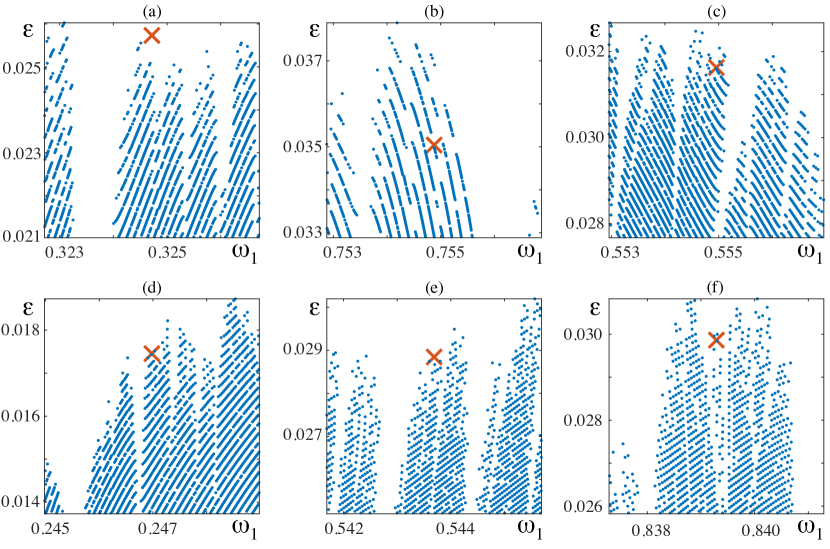
Figure 19: Tori in the $(\omega_{1},\varepsilon)$ plane, near $\varepsilon_{c}(\omega^{*})$ for the six vectors $\omega^{*}$ in Table 4. Each point represents a torus at a fixed $\delta=\delta_{c}$ that passes through the corresponding critical point. In each figure, the (red) X marks the location of the associated critical torus. The frequencies corresponding to nearby tori (blue) are computed on a grid with spacing $10^{-4}$ in $\omega_{1}$ and $4(10)^{-5}$ in $\varepsilon$.

While it is not possible to compute whether these tori are locally most robust on arbitrarily small neighborhoods, we can quantify the degree to which they fail to be local maxima on a fixed small interval in $\omega_{1}$, fixing a cross-section $\delta=\delta_{c}$ that passes through the corresponding critical point. We compute rotational tori for values of $y$ near $y_{c}$ such that the spacing of $\omega_{1}$ values is approximately $10^{-4}$ (i.e., using the $\varepsilon=0$ approximation for $y$ and $\delta$), and the $\varepsilon$ spacing is $4(10)^{-5}$ with $\varepsilon\leq\varepsilon_{c}+0.005$. Of these, we consider only tori with $|\omega_{1}-\omega_{1}^{*}|<0.002$, and which are more robust than $\omega^{*}$. These tori correspond to the points in Fig. 19 that lie above $\varepsilon_{c}(\omega^{*})$, which is indicated by the (red) X in each panel.

	$\omega^{*}$	$\varepsilon_{c}$	$y_{c}$	$\delta_{c}$	#M.R.
(a)	$(\sigma-1,\sigma^{-1})$	$0.025731358271922$	$-0.300341913511639$	$-0.581991952776833$	3
(b)	$(\sigma^{-1},\sigma-1)$	$0.035042379103690$	$0.137249321586741$	$-0.285775646047323$	180
(c)	$(\alpha^{2}-1,\alpha-1)$	$0.031629688390353$	$-0.046265357816195$	$-0.237775229395970$	61
(d)	$(\alpha-1,\alpha^{2}-1)$	$0.017453913097431$	$-0.374459102422933$	$-0.279201189795316$	92
(e)	$(\tau-1,\tau^{-1})$	$0.029861717573837$	$-0.444144360895140$	$0.203236055553548$	47
(f)	$(\tau^{-1},\tau-1)$	$0.028845453269968$	$-0.826759694950616$	$-0.103754031724428$	44

Table 4: Critical parameters for tori in cubic fields with discriminants $-23$, $49$ and $-44$, recall (22), (29), and (32). The labels (a)-(f) indicate the corresponding panel in Fig. 19. For each field, two rotation vectors $\omega^{*}$ are chosen, related by permutation. The torus ${\cal T}_{\omega^{*}}(\varepsilon,y,\delta)$ breaks up at $\varepsilon_{c}$ and is located at $(y_{c},\delta_{c})$. The final column shows the number of tori that are more robust among the tori computed in an interval $|\omega_{1}-\omega_{1}^{*}|<0.002$ with $\omega_{1}$ spacing of $10^{-4}$ and $\varepsilon<\varepsilon_{c}+0.005$ with spacing of $4(10)^{-5}$.

One measure of local robustness is the distance, $\Delta\omega=|\omega_{1}-\omega_{1}^{*}|$, to the closest, more robust torus. The first spiral mean vector, (a) in the table and figure, has a distance of $\Delta\omega\sim 2(10)^{-3}$; this makes it five-times more robust than than (e), the first $D=-44$ torus, and more than 25-times more robust than all others. By this measure the frequency (b) in $D=-23$, is least robust since there is a more robust torus within $\Delta\omega\sim 4(10)^{-6}$. This measure best matches what is observed by eye in Fig. 19, where similarly (a) and (e) appear the most locally robust within a single peak of the each panel.

Another measure of robustness is the distance $\Delta\varepsilon=\varepsilon_{c}(\omega)-\varepsilon_{c}(\omega^{*})$ for the most robust computed torus in the interval. By this measure, the first vector, (a), is more robust in the sense that for this torus $\Delta\varepsilon\sim 3(10)^{-4}$, and this value is at least three-times smaller than that for any of the other tori. Torus (b), the second spiral mean case, is the least robust with $\Delta\varepsilon$ more than nine-times larger than the value for (a).

Finally, the last column of Table 4, labeled #M.R., lists the number of more robust tori within the computed frequency interval. Again by this measure the first spiral mean, (a), is the most robust since the number is least 14-times smaller than any other number. The second spiral mean, (b), is the least robust with $180$ nearby, more robust tori.

From these results, though none of the six vectors considered is locally robust over a large range, both (a) and (e) could be considered locally robust, and the first spiral mean case, (a), is the most robust over the range we have considered. This perhaps provides some indication that the spiral field remains the best candidate to generalize the noble numbers. Nevertheless, since there are a countably infinite number of vectors in each field, we cannot rule out that another representative would behave more robustly.

7 Conclusions

In this paper we develop criteria to distinguish orbits that lie on rotational two-tori from those that are chaotic or resonant, as well as to compute rotation vectors for the rotational two-tori. Our model is a three-dimensional, volume-preserving map (1) with frequency map and force (6), and the primary tools are the weighted Birkhoff average (10) and an algorithm for calculating resonance order, Algorithm 1.

To distinguish chaotic from regular orbits and calculate rotation vectors, we use the weighted Birkhoff average. Computation of the rotation vector of the tori to at least 11-digit accuracy required $2T=2(10)^{6}$ iterates of the map—the second half of the iterates being used to estimate the error (13). However in most cases as we saw in Fig. 3, many fewer iterates—say $3(10)^{4}$—would be sufficient to obtain this accuracy and to distinguish regular from chaotic dynamics. Moreover, as we previously showed in [SM20], the weighted Birkhoff average is more efficient than other techniques, such as fast Lyapunov methods, for this distinction.

To distinguish tori from resonances, it was important to use “linear approximations” rather than the often-used simultaneous approximations to the vector $\omega$: we look for the closest resonant line (5) to the computed rotation number in the sense of Euclidean distance (20). Unlike the case of a single frequency (where the Stern-Brocot tree is the optimal method [SM20]), there seems to be no general theory that gives a “fast” method for determining optimal linear approximations. The general theory of optimal resonance order is not completely understood, though the scaling of resonance order with tolerance that is seen in Fig. 9 is what would be expected from the theorems of Dirichlet and Minkowski (see App. A).

To compute resonance order to a precision $\rho$ we use a brute force method, recall Algorithm 1, and unfortunately, this is a substantial part of the computational cost in our method (about 50% of the effort). Nevertheless, is important to find such linear approximations to eliminate dynamical resonances; such orbits lie on regular tori that are not “rotational”, instead these enclose isolated invariant circles of the map (if they exist [DM12]).

After finding rotational tori, in §5 and §6 we use a variety of methods, including simultaneous approximations and parameter continuation to study the most robust tori, and to test conjectures regarding the robustness of tori with rotation vectors in three cubic fields. Since the number of tori studied here is relatively small (compared to the number tested to find the locally robust rotational tori), we also use, in §5.2, a brute force method to compute the sequence of best simultaneous approximations to $\omega$, e.g., the sequence of “periods” (34) of a rotation vector. Note that, by contrast with linear approximations, there is a fast method for computing the simultaneous approximation sequence [Cla97].

Our results indicate that frequencies of robust tori are discernibly different from random frequency vectors, see Fig. 16, but as in [FM13], we have been unable to extract a simple number-theoretic property for the globally most robust tori and the Diophantine constant sequence does not seem to have a simple behavior, Fig. 15. There is only weak evidence for local robustness of conjectured, low-discriminant cubic fields, and in particular while some of the elements in the three conjectured cubic fields may be locally robust, none of them seem to be associated with the most robust tori in the same way that the noble numbers are associated with most robust and locally robust invariant circles for 2D maps.

Our results for computing tori should be compared with previous techniques that used periodic orbits to approximate the torus and Greene’s residue criterion to estimate their breakup. Greene’s residue is certainly the optimal method for area-preserving maps with a time-reversal symmetry: it can easily give highly accurate breakup thresholds for an invariant circle [Mac83]. As was shown in [FM13], this idea can be generalized to the volume-preserving case studied in the current paper because it does have a time-reversal symmetry, which permits the computation of sequences of symmetric periodic orbits. In [FM13], orbits with periods of order $10^{4}$ were used to obtain estimates of breakup thresholds with a relative error in $\varepsilon_{c}$ that was estimated to be $0.002$. The results obtained in the current paper show that these thresholds were slight over-estimates of $\varepsilon_{c}(\omega)$, and allow us to refine the breakup threshold to a relative error of about $4(10)^{-8}$. This relies on the ad hoc criterion (15), that declares that the orbit has become chaotic when the accuracy of the weighted Birkhoff average drops below our threshold of $11$-digits (of course, there is a similar, ad hoc threshold for the residue criterion). Note, however that the rapid decrease of ${dig^{(T)}}$ over a narrow parameter range, as seen in Fig. 18, is a clear signal of the torus destruction.

Another advantage of the weighted Birkhoff method used here is that it can be applied to asymmetric maps (as we did for 2D in [SM20]), and does not rely on any sophisticated method to find periodic orbits that are simultaneous rational approximations to a given incommensurate frequency vector. Moreover, even though the residue method works very well in 2D and is successful in 3D, it has not led to accurate methods that can estimate the breakup thresholds for tori in 4D symplectic maps. One of the problems for the 4D case is that there are multiple “partial traces” of a symplectic matrix needed to define a stability threshold. Such considerations are irrelevant for weighted Birkhoff averages.

In the future, we plan to continue the study of two-tori for maps in three and possibly four dimensions. The fast convergence for the weighted Birkhoff method makes it well suited for extended precision computations as noted in [DSSY17]. We have successfully performed test cases for one- and two-dimensional tori in phase spaces of dimensions one, two, and three. In future work, we plan to explore such high precision calculations in the hope that extracting more digits will lead to a better number theoretic understanding of the properties of the rotation vectors for robust tori.

Appendix A Diophantine Constants

There are two common ways in which a vector $\omega\in{\mathbb{R}}^{d}$ can be approximated by rationals. The first, simultaneous approximation, seeks a vector $(p,q)\in{\mathbb{Z}}^{d}\times{\mathbb{N}}$ that corresponds to a nearby rational, i.e., $\omega\approx\frac{p}{q}$. The second, linear approximation, seeks an integer vector $(m,n)\in{\mathbb{Z}}^{d}\setminus\{0\}\times{\mathbb{Z}}$, that corresponds to a nearby resonance, i.e., $m\cdot\omega-n\approx 0$.

Define the pseudo-norm

$${\|{\omega}\|_{\mathbb{Z}}}=\inf_{p\in{\mathbb{Z}}^{d}}\|\omega-p\|_{\infty}$$ (33)

that computes the distance to the nearest point on an integer grid. Lochak [Loc92] defines the periods, $q_{i}$ of $\omega$ as the sequence of positive integers so that, $q_{0}=1$, and $\forall q<q_{i+1}$,

$${\|{q_{i}\omega}\|_{\mathbb{Z}}}\leq{\|{q\omega}\|_{\mathbb{Z}}}.$$ (34)

Thus if $p_{i}$ is the integer vector such that ${\|{q_{i}\omega}\|_{\mathbb{Z}}}=\|q_{i}\omega-p_{i}\|_{\infty}$, then $\frac{p_{i}}{q_{i}}$ are (strong) best approximants of $\omega$.

Similarly we can define a set of nearest resonances to $\omega$ as a sequence of nonzero integer vectors $m_{i}$ so that $m_{0}=(1,...,1)$ and whenever $0<\|m\|\leq\|m_{i+1}\|$ then

$${\|{m_{i}\cdot\omega}\|_{\mathbb{Z}}}\leq{\|{m\cdot\omega}\|_{\mathbb{Z}}},\quad m,m_{i}\in{\mathbb{Z}}^{d}\setminus\{0\}$$

The sequence of resonance orders, $\|m_{i}\|_{1}=M_{i}$ thus obtained is unique, even though the resonant sequence itself may not be.

Theorems of Dirichlet and Minkowski, give a bound on the goodness of these approximations:

Theorem 1 ([Bak84, Cas57, Sch91]).

For any $\omega\in{\mathbb{R}}^{d}$ and for any $K>0$, there exist $(m,n)\in{\mathbb{Z}}^{d}\setminus\{0\}\times{\mathbb{Z}}$ with $\|m\|_{\infty}\leq K$ such that

$$|m\cdot\omega-n|<\frac{1}{K^{d}}.$$ (35)

Similarly whenever at least one $\omega_{i}$ is irrational, then for any $Q>0$, there exist $0<|q|\leq Q$ and $p\in{\mathbb{Z}}^{d}$ such that

$$\|q\omega-p\|^{d}_{\infty}<\frac{1}{Q}.$$ (36)

In (35) we say that $(m,n)$ is a “near” resonance for $\omega$ and, for (36), that the vector $p/q$ is a “good” rational approximation to $\omega$. Note the complementary placement of the $d^{th}$ power in these two expressions.

Based on these complementary notions of approximation, there are also two senses in which $\omega$ can be strongly “irrational”, or Diophantine. Defining the linear and simultaneous “closeness” parameters

$$c_{l}(\omega,m) =\|m\|^{d}_{\infty}{\|{m\cdot\omega}\|_{\mathbb{Z}}},$$ (37)

$$c_{s}(\omega,q) =q\|q\omega\|^{d}_{\mathbb{Z}},$$

then the associated Diophantine constants are

$$c_{l}(\omega) =\liminf_{\|m\|_{\infty}\to\infty}c_{l}(\omega,m),$$ (38)

$$c_{s}(\omega) =\liminf_{q\to\infty}c_{s}(\omega,q).$$

A vector $\omega$ is (linear, simultaneous) Diophantine if $c_{l,s}(\omega)>0$. A theorem of Dirichlet implies that if $\theta$ is an algebraic irrational of degree $d+1$, then for $\omega=(\theta,\theta^{2},\ldots,\theta^{d})$, $c_{s}(\omega)>0$; thus the vector $\omega$ is (simultaneous) Diophantine. For example, every quadratic irrational is Diophantine for $d=1$.

Note that, by Th. 1, $c_{l},c_{s}\leq 1$. When $d=1$ these constants are trivially equal and it is known that for any $\omega$, $c_{s}(\omega)\leq c_{s}(\phi)=\frac{1}{\sqrt{5}}$, where $\phi$ is the golden mean [HW79, Thm. 194]. As noted in [Loc92], for $d=2$ it has been proven by Davenport that the upper bounds on $c_{l}$ and $c_{s}$ over $\omega\in{\mathbb{R}}^{2}$ are the same, and that these upper bounds are at least $\tfrac{2}{7}$. Furthermore, Adams showed that there are integral bases for cubic fields for which $c_{s}(\omega)=\tfrac{2}{7}$. It been conjectured that for any $\omega$, $c_{s}\leq\tfrac{2}{7}$, and that the only numbers for which $c_{s}$ is near $\tfrac{2}{7}$ are integral bases of a real cubic field [Cus74]. Indeed Cusick conjectures that there is an integral basis for the discriminant $49$ field (28) that achieves this value.

Computation of the sequence of periods (36) can be done efficiently using algorithms developed by Clarkson [Cla97], and this would be especially important if high precision computations are required to attempt to estimate the asymptotic Diophantine constant. We simply use the brute force method of computing $\|q\omega\|_{Z}$ for each natural number up to some $Q$. The resulting sequence of periods and approximations to the Diophantine constant for the vector (29) are shown in Table 5. A comparison between several cubic irrationals is shown in Fig. 15(a).

Note that if we know $\omega$ to precision $\rho$, then $c_{s}(\omega,q)$ can be computed with precision $q\rho$. Using the cutoff ${dig^{(T)}}=11$, this implies that periods must be limited so that $q\ll 10^{11}$, e.g., $q\lesssim 10^{7}$ so that $c_{s}$ can be computed with 4 digit accuracy.

$p_{1}$	$p_{2}$	$q$	$\|q\omega\|_{Z}$	$c_{s}(\omega,q)$
1	0	1	0.445041867912628	0.198062264195161
2	1	3	0.335125603737885	0.336927510842046
2	1	4	0.219832528349486	0.193305362082111
7	3	13	0.214455717135830	0.597886309959160
9	4	16	0.120669886602055	0.232979544520846
11	5	20	0.099162641747430	0.196664590366583
36	16	65	0.072278585679150	0.339572606605588
45	20	81	0.048391300922901	0.189679158405874
146	65	263	0.046011261021278	0.556780505022018
182	81	328	0.026267324657880	0.226310929055850
227	101	409	0.022123976265050	0.200193363242583
737	328	1328	0.015600587970539	0.323206442195226
919	409	1656	0.010666736687313	0.188418473697497
2984	1328	5377	0.009876233796604	0.524472547765830
3721	1656	6705	0.005724354173708	0.219710986884052
4640	2065	8361	0.004942382513946	0.204235358627254
15066	6705	27148	0.003369907963133	0.308300280752348
18787	8361	33853	0.002354446209210	0.187661294078270
61001	27148	109920	0.002120956116414	0.494470156865191
76067	33853	137068	0.001248951841262	0.213809728033248

Table 5: Best approximants for (29), a vector in the $D=49$ cubic field.

Appendix B Cubic fields and Jacobi-Perron

An algebraic field is an extension of ${\mathbb{Q}}$ to include some family of algebraic numbers. Consider the monic polynomial

$$p(x)=x^{3}-kx^{2}-lx-m$$ (39)

for $k,l,m\in{\mathbb{Z}}$ and $m\neq 0$. A root, $\tau$ of such a polynomial is an algebraic integer and generates a cubic field ${\mathbb{Q}}[\tau]=\{a+b\tau+c\tau^{2}:a,b,c\in{\mathbb{Q}}\}$. The integers in such a field correspond to the restriction of $a,b,c\in{\mathbb{Z}}$. An integral basis of such a field is a vector $(1,\tau,\sigma)$ that generates the integers. The fields can be characterized by the discriminant, $D=k^{2}l^{2}-4k^{3}m+4l^{3}-18klm-27m^{2}$ of the polynomial (39). When $D<0$ there are two complex roots and when $D>0$ all the roots are real.

The cubic field with the smallest $|D|$ is that of the spiral mean, which has $D=-23$, the minimal polynomial (39) with $(k,l,m)=(0,1,1)$ with real root $\sigma$, and integral basis $(1,\sigma,\sigma^{2})$. Siegel showed this root is the smallest Pisot number (an algebraic number that is the unique root of its minimal polynomial outside the unit circle) [Sie44]. We have used the fact that, for the vector $\omega$ in (22), $(1,\omega)$ forms an integral basis for ${\mathbb{Q}}[\sigma]$. An alternative polynomial for this field has $(k,l,m)=(-1,0,1)$. The real root in this case is $\sigma^{-1}$.

When $m=1$, and $\tau$ is a Pisot number, Tompaidis noted that there is an integral basis of the cubic field for which the Jacobi-Perron algorithm (JPA), a generalization of the continued fraction, is periodic. Given a vector $\omega\in[0,1]^{2}$ the JPA generates a sequence of integer vectors $r_{i}=(p_{i},q_{i})\in{\mathbb{N}}^{3}$ so that $p_{i}/q_{i}$ is a rational approximation to $\omega$ and these vectors obey a recursion

$$r_{n+1}=k_{n+1}r_{n}+l_{n+1}r_{n-1}+r_{n-2}.$$

The coefficients $(k_{n},l_{n})$ of this recursion are determined by iterating the map

$$\omega \mapsto\left(\frac{1}{\omega_{2}},\frac{\omega_{1}}{\omega_{2}}\right)-(k,l),$$ (40)

$$(k,l) =\left(\left\lfloor\frac{1}{\omega_{2}}\right\rfloor,\left\lfloor\frac{\omega_{1}}{\omega_{2}}\right\rfloor\right).$$

The algorithm is initialized with $r_{-2}=(0,1,0)$, $r_{-1}=(1,0,0)$ and $r_{0}=(0,0,1)$. We give the resulting expansions for several frequency vectors in the first four cubic fields in Table 6. Here the sequences $(k_{n},l_{n})$ are always eventually periodic, with the repeated portion enclosed in $[\,]$. For example the first spiral mean case gives a period-two sequence.

$D$	$p(x)$	Root	$\omega$	Jacobi-Perron
$-23$	$x^{3}-x-1$	$1.324717957244745$	$(\sigma-1,\sigma^{-1})$	$\left[{\begin{pmatrix}{1}\\ {0}\end{pmatrix}},{\begin{pmatrix}{2}\\ {0}\end{pmatrix}}\right]$
			$(\sigma^{-1},\sigma-1)$	${\begin{pmatrix}{3}\\ {2}\end{pmatrix}},\left[{\begin{pmatrix}{2}\\ {0}\end{pmatrix}},{\begin{pmatrix}{4}\\ {0}\end{pmatrix}}\right]$
$-31$	$x^{3}-x^{2}-1$	$1.465571231876768$	$(\kappa-1,\kappa^{-1})$	$\left[{\begin{pmatrix}{1}\\ {0}\end{pmatrix}}\right]$
			$(\kappa^{-1},\kappa-1)$	${\begin{pmatrix}{2}\\ {1}\end{pmatrix}},\left[{\begin{pmatrix}{2}\\ {0}\end{pmatrix}},{\begin{pmatrix}{3}\\ {0}\end{pmatrix}}\right]$
$-44$	$x^{3}-x^{2}-x-1$	$1.839286755214161$	$(\tau-1,\tau^{-1})$	$\left[{\begin{pmatrix}{1}\\ {1}\end{pmatrix}}\right]$
			$(\tau^{-1},\tau-1)$	${{\begin{pmatrix}{1}\\ {0}\end{pmatrix}}}^{2},{\begin{pmatrix}{3}\\ {1}\end{pmatrix}},\left[{\begin{pmatrix}{1}\\ {0}\end{pmatrix}},{{\begin{pmatrix}{2}\\ {0}\end{pmatrix}}}^{3},{\begin{pmatrix}{1}\\ {0}\end{pmatrix}},{\begin{pmatrix}{4}\\ {0}\end{pmatrix}}\right]$
$49$	$x^{3}+x^{2}-2x-1$	$1.246979603717467$	$(\alpha-1,\alpha^{-1})$	$\left[{\begin{pmatrix}{1}\\ {0}\end{pmatrix}},{\begin{pmatrix}{3}\\ {0}\end{pmatrix}}\right]$
			$(\alpha^{-1},\alpha-1)$	${\begin{pmatrix}{1}\\ {0}\end{pmatrix}},{\begin{pmatrix}{2}\\ {1}\end{pmatrix}},\left[{\begin{pmatrix}{1}\\ {0}\end{pmatrix}},{\begin{pmatrix}{3}\\ {0}\end{pmatrix}}\right]$
			$(\alpha-1,\alpha^{2}-1)$	${\begin{pmatrix}{4}\\ {2}\end{pmatrix}},\left[{\begin{pmatrix}{4}\\ {0}\end{pmatrix}},{\begin{pmatrix}{5}\\ {0}\end{pmatrix}}\right]$

Table 6: Jacobi-Perron sequences for vectors in the four cubic fields with $|D|<50$. The last column shows the sequence generated by (40). All are eventually periodic, and the periodic portions are enclosed in brackets.

There are two cases in the table for which the sequences are period-one, analogous to the golden mean for the ordinary continued fraction. The resulting sequences are then the values $(k,l)$ in the polynomial (39) with $m=1$. In order for this to occur, the root must be a Pisot number, with $k<\tau<k+1$ and one must choose $\omega=(\tau-k,\tau^{-1})$. Following Tompaidis, we might think of these vectors as generalized versions of the golden mean.

More generally it is known there are only finitely many periodic JPA sequences associated with each unit in an algebraic field [AR11]. When $d=1$, every eventually periodic continued fraction is a quadratic irrational; however, it is apparently not known how to characterize the vectors that have eventually periodic JPA sequences.

References

- [AC15] C. V. Abud and I. L. Caldas. On Slater’s criterion for the breakup of invariant curves. Physica D, 308:34–39, 2015. https://doi.org/10.1016/j.physd.2015.06.005.
- [ACP06] E.G. Altmann, G. Cristadoro, and D. Paz. Nontwist non-Hamiltonian systems. Phys. Rev. E, 73(5):056201, 2006. http://link.aps.org/abstract/PRE/v73/e056201.
- [ACS92] R. Artuso, G. Casati, and D.L. Shepelyansky. Break-up of the spiral mean torus in a volume-preserving map. Chaos, Solitons & Fractals, 2(2):181–190, 1992. https://doi.org/10.1016/0960-0779(92)90007-A.
- [AR11] B. Adam and G. Rhin. Periodic Jacobi-Perron expansions associated with a unit. J. Théorie des Nombres de Bordeaux, 23(3):527–539, 2011. http://www.jstor.org/stable/44011250.
- [Bak84] A. Baker. A Concise Introduction to the Theory of Numbers. Cambridge Univ. Press, Cambridge, 1984.
- [BM93] E.M. Bollt and J.D. Meiss. Breakup of invariant tori for the four-dimensional semi-standard map. Physica D, 66(3&4):282–297, 1993. https://doi.org/10.1016/0167-2789(93)90070-H.
- [BM94] C. Baesens and R.S. MacKay. The one to two-hole transition in cantori. Physica D, 71:372–389, 1994. https://doi.org/10.1016/0167-2789(94)90005-1.
- [Cas57] J.W.S Cassels. An Introduction to Diophantine Approximation. Cambridge University Press, Cambridge, 2nd printing edition, 1957.
- [Chi79] B.V. Chirikov. A universal instability of many-dimensional oscillator systems. Phys. Rep., 52(5):263–379, 1979. https://doi.org/10.1016/0370-1573(79)90023-1.
- [Cla97] L.V. Clarkson. Approximation of Linear Forms by Lattice Points with Applications to Signal Processing. PhD thesis, Australian National University, 1997.
- [CS90] C.-Q. Cheng and Y.-S. Sun. Existence of periodically invariant curves in 3-dimensional measure-preserving mappings. Celestial Mech. and Dyn. Astron., 47:293–303, 1990. https://doi.org/10.1007/BF00053457.
- [Cus72] T.W. Cusick. Formulas for some Diophantine approximation constants. Math. Ann., 197:182–188, 1972. https://doi.org/10.1007/BF01428224.
- [Cus74] T.W. Cusick. The two-dimensional Diophantine approximation constant. Monatshefte für Mathematik, 78:297–304, 1974. https://doi.org/10.1007/BF01294641.
- [DDS+16] S. Das, C.B. Dock, Y. Saiki, M. Salgado-Flores, E. Sander, J. Wu, and J.A. Yorke. Measuring quasiperiodicity. Euro. Phys. Lett., 114:40005, 2016. https://doi.org/10.1209/0295-5075/114/40005.
- [DM12] H.R. Dullin and J.D. Meiss. Resonances and twist in volume-preserving mappings. SIAM J. Appl. Dyn. Sys., 11:319–349, 2012. https://doi.org/10.1137/110846865.
- [DSSY16] S. Das, Y. Saiki, E. Sander, and J.A. Yorke. Quasiperiodicity: Rotation numbers. In C. Skiadas, editor, The Foundations of Chaos Revisited: From Poincaré to Recent Advancement, Understanding Complex Systems. Springer, Cham, 2016. https://doi.org/10.1007/978-3-319-29701-9_7.
- [DSSY17] S. Das, Y. Saiki, E. Sander, and J.A. Yorke. Quantitative quasiperiodicity. Nonlinearity, 30(11):4111, 2017. https://doi.org/10.1088/1361-6544/aa84c2.
- [DY18] S. Das and J.A. Yorke. Super convergence of ergodic averages for quasiperiodic orbits. Nonlinearity, 31(2):491–501, 2018. https://doi.org/10.1088/1361-6544/aa99a0.
- [EV01] K. Efstathiou and N. Voglis. A method for accurate computation of the rotation and twist numbers for invariant tori. Physica D, 158:151–163, 2001. https://doi.org/10.1016/S0167-2789(01)00299-8.
- [FM13] A.M. Fox and J.D. Meiss. Greene’s residue criterion for the breakup of invariant tori of volume-preserving maps. Physica D, 243(1):45–63, 2013. https://doi.org/10.1016/j.physd.2012.09.005.
- [FM16] A.M. Fox and J.D. Meiss. Computing the conjugacy of invariant tori for volume-preserving maps. SIAM J. Appl. Dyn. Sys., 15(1):557–579, 2016. http://epubs.siam.org/doi/abs/10.1137/15M1022859.
- [FS73] C. Froeschlé and J.P. Scheidecker. Numerical study of a four dimensional mapping II. Astron. and Astrophys., 22:431–436, 1973. http://adsabs.harvard.edu/abs/1973A%26A....22..431F.
- [FWAM06] K. Fuchss, A. Wurm, A. Apte, and P.J. Morrison. Breakup of shearless meanders and “outer” tori in the standard nontwist map. Chaos, 16:033120, 2006. https://doi.org/10.1063/1.2338026.
- [GMS10] G. Gómez, J.M. Mondelo, and C Simó. A collocation method for the numerical Fourier analysis of quasi-periodic functions. I: Numerical tests and examples. Discrete Contin. Dyn. Syst. Ser. B, 14:41–74, 2010. https://doi.org/10.3934/dcdsb.2010.14.41.
- [Gre79] J.M. Greene. A method for determining a stochastic transition. J. Math. Phys., 20:1183–1201, 1979. https://doi.org/10.1063/1.524170.
- [HCF+16] A. Haro, M. Canadell, J-L Figueras, A.-L. Josep, and M. Mondelo. The Parameterization Method for Invariant Manifolds from Rigorous Results to Effective Computations. Springer International, 2016. https://doi.org/10.1007/978-3-319-29662-3.
- [HM88] B. Hu and J.M. Mao. Transitions to chaos in higher dimensions. In B.L. Hao, editor, Directions in Chaos, volume 1, pages 206–271. World Scientific, Singapore, 1988.
- [HW79] G.H. Hardy and E.M. Wright. An Introduction to the Theory of Numbers. Oxford Univ. Press, Oxford, 1979.
- [KM89] H.-t. Kook and J.D. Meiss. Periodic-orbits for reversible, symplectic mappings. Physica D, 35(1-2):65–86, 1989. https://doi.org/10.1016/0167-2789(89)90096-1.
- [KO86] S. Kim and S. Ostlund. Simultaneous rational approximations in the study of dynamical systems. Phys. Rev. A, 34:3426–3434, 1986. https://doi.org/10.1103/PhysRevA.34.3426.
- [LFC92] J. Laskar, C. Froeschlé, and A. Celletti. The measure of chaos by the numerical analysis of the fundamental frequencies. Application to the standard mapping. Physica D, 56:253–269, 1992. https://doi.org/10.1016/0167-2789(92)90028-L.
- [LM10] Z. Levnajić and I. Mezić. Ergodic theory and visualization. I. Mesochronic plots for visualization of ergodic partition and invariant sets. Chaos, 20(3):033114, 2010. https://doi.org/10.1063/1.3458896.
- [Loc92] P. Lochak. Canonical perturbation theory via simultaneous approximation. Russ. Math. Surveys, 47(6):59–140, 1992. https://doi.org/10.1070/RM1992v047n06ABEH000965.
- [LV09] A. Luque and J. Villanueva. Numerical computation of rotation numbers of quasi-periodic planar curves. Physica D, 238(20):2025–2044, 2009. https://doi.org/10.1016/j.physd.2009.07.014.
- [LV14] A. Luque and J. Villanueva. Quasi-periodic frequency analysis using averaging-extrapolation methods. SIAM J. Dyn.Sys., 13(1):1–46, 2014. https://doi.org/10.1137/130920113.
- [Mac83] R.S. MacKay. A renormalisation approach to invariant circles in area-preserving maps. Physica D, 7:283–300, 1983. https://doi.org/10.1016/0167-2789(83)90131-8.
- [May88] D.H. Mayer. On the distribution of recurrence times in nonlinear systems. Lett. Math. Phys., 16(2):139–143, 1988. https://doi.org/10.1007/BF00402021.
- [Mei12] J.D. Meiss. The destruction of tori in volume-preserving maps. Comm. Nonl. Sci. Numer. Simul., 17:2108–2121, 2012. https://doi.org/10.1016/j.cnsns.2011.04.014.
- [MS91] S. Marmi and J. Stark. On the standard map critical function. Nonlinearity, 5(3):743–761, 1991. https://doi.org/10.1088/0951-7715/5/3/007.
- [MS92] R.S. MacKay and J. Stark. Locally most robust circles and boundary circles for area-preserving maps. Nonlinearity, 5:867–888, 1992. http://iopscience.iop.org/0951-7715/5/4/002.
- [Sch91] W.M. Schmidt. Diophantine Approximations and Diophantine Equations, volume 1467 of Lect. Notes in Math. Springer-Verlag, New York, 1991. https://doi.org/10.1007/BFb0098246.
- [Sie44] C.L. Siegel. Algebraic integers whose conjugates lie in the unit circle. Duke Math. J., 11:597–602, 1944. https://doi.org/10.1215/S0012-7094-44-01152-X.
- [SM20] E. Sander and J. D. Meiss. Birkhoff averages and rotational invariant circles for area-preserving maps. Physica D, 411:132569, 2020. https://doi.org/10.1016/j.physd.2020.132569.
- [SMS+18] M.S. Santos, M. Mugnaine, J.D. Szezech, A.M. Batista, I.L. Caldas, M.S. Baptista, and R.L. Viana. Recurrence-based analysis of barrier breakup in the standard nontwist map. Chaos, 28(8):085717, 2018. https://doi.org/10.1063/1.5021544.
- [SMS+19] M.S. Santos, M. Mugnaine, J.D. Szezech, A.M. Batista, I.L. Caldas, and R.L. Viana. Using rotation number to detect sticky orbits in Hamiltonian systems. Chaos, 29(4):043125, 2019. https://doi.org/10.1063/1.5078533.
- [SSC+13] J.D. Szezech, A.B. Schelin, I.L. Caldas, S R. Lopes, P.J. Morrison, and R.L. Viana. Finite-time rotation number: A fast indicator for chaotic dynamical structures. Phys. Lett. A, 377:452–456, 2013. https://doi.org/10.1016/j.physleta.2012.12.013.
- [Ste96] I. Stewart. Tales of a neglected number. Sci. Am., 274(6):102–103, 1996. https://doi.org/10.1038/scientificamerican0696-102.
- [SV06] T.M. Seara and J. Villanueva. On the numerical computation of Diophantine rotation numbers of analytic circle maps. Physica D, 217(2):107–120, 2006. https:/doi.org/10.1016/J.Physd.2006.03.013.
- [Tom96] S. Tompaidis. Numerical study of invariant sets of a quasiperiodic perturbation of a symplectic map. Experiment. Math., 5:211–230, 1996. https://doi.org/10.1080/10586458.1996.10504589.
- [VBK96] M.N. Vrahatis, T.C. Bountis, and M. Kollmann. Periodic orbits and invariant surfaces of 4d nonlinear mappings. Int. J. Bif. and Chaos, 6(8):1425–1437, 1996. https://doi.org/10.1142/s0218127496000849.
- [Wal12] M. Waldschmidt. Recent advances in Diophantine approximation. In D. Goldfeld, J. Jorgenson, J. Jones, D. Ramakrishnan, K. Ribet, and J. Tate, editors, Number Theory, Analysis and Geometry, pages 659–704. Springer, Boston, MA, 2012. https://doi.org/10.1007/978-1-4614-1260-1.
- [Xia92] Z. Xia. Existence of invariant tori in volume-preserving diffeomorphisms. Erg. Th. Dyn. Sys., 12(3):621–631, 1992. https://doi.org/10.1017/S0143385700006969.
- [ZHS01] J.L. Zhou, B. Hu, and Yi-Sui Sun. Universal behaviour on the break-up of the spiral mean torus. Chin. Phys. Lett, 18(12):1550–1553, 2001. https://doi.org/10.1088/0256-307X/18/12/303.
- [ZTRK07] Y. Zou, M. Thiel, M.C. Romano, and J. Kurths. Characterization of stickiness by means of recurrence. Chaos, 17:043101, 2007. http://link.aip.org/link/?CHAOEH/17/043101/1.