Dynamic Connectivity in Disk Graphs

Abstract

Let $S$ be a set of sites, each associated with a point in $\mathbb{R}^{2}$ and a radius $r_{s}$ and let $\mathcal{D}(S)$ be the intersection graph of the disks defined by the sites and radii. We consider the problem of designing data structures that maintain the connectivity structure of $\mathcal{D}(S)$ while allowing the insertion and deletion of sites. We denote the size of $S$ by $n$.

For unit disk graphs we describe a data structure that has $O(\log^{2}n)$ amortized update time and $O(\frac{\log n}{\log\log n})$ amortized query time. For disk graphs where the ratio $\Psi$ between the largest and smallest radius is bounded, we consider the decremental and the incremental case separately, in addition to the fully dynamic case. In the fully dynamic case we achieve amortized $O(\Psi\lambda_{6}(\log n)\log^{9}n)$ update time and $O(\log n)$ query time, where $\lambda_{s}(n)$ is the maximum length of a Davenport-Schinzel sequence of order $s$ on $n$ symbols. This improves the update time of the currently best known data structure by a factor of $\Psi$ at the cost of an additional $O(\log\log n)$ factor in the query time. In the incremental case we manage to achieve a logarithmic dependency on $\Psi$ with a data structure with $O(\alpha(n))$ query and $O(\log\Psi\lambda_{6}(\log n)\log^{9}n)$ update time.

For the decremental setting we first develop a new dynamic data structure that allows us to maintain two sets $B$ and $P$ of disks, such than at a deletion of a disk from $B$ we can efficiently report all disks in $P$ that no longer intersect any disk of $B$. Having this data structure at hand, we get decremental data structures with an amortized query time of $O(\frac{\log n}{\log\log n})$ supporting $m$ deletions in $O((n\log^{5}n+m\log^{9}n)\lambda_{6}(\log n)+n\log\Psi\log^{4}n)$ overall time for bounded radius ratio $\Psi$ and $O((n\log^{6}n+m\log^{10}n)\lambda_{6}(\log n))$ for general disk graphs.

1 Introduction

Preprocessing a graph $G$ in such a way that one can efficiently determine if two vertices lie in the same connected component is a fundamental problem in algorithmic graph theory. If the graph is static, using a breadth first search or depth first search to identify all connected components allows to answer these queries in $O(1)$ time after a linear preprocessing time. If the graph is dynamic, the situation is more complicated. In such a dynamic graph the connectivity queries are interleaved with update operations on the graph. When having a fixed set of vertices and allowing only the insertion of edges, using a disjoint-set data structure solves the problem. Such a data structure can be implemented efficiently to achieve optimal amortized time of $O(1)$ for updates and $O(\alpha(n))$ for queries, where $\alpha(n)$ is the inverse Ackermann function [24]. For completeness, this data structure is described in Theorem 2.1.

If both edge insertions and deletions are allowed, Holm et al. [19] described the fastest currently known data structure for general graphs. The data structure achieves amortized $O(\frac{\log n}{\log\log n})$ update time and $O(\log^{2}n)$ amortized time for edge updates. For planar graphs, Eppstein et al. [14] give a data structure with $O(\log n)$ amortized time for both queries and updates. If the vertex set is considered to be dynamic, this is done by having a fixed base set of $m$ edges and activating or deactivating vertices and their incident edges. In this setting, there is a data structure allowing vertex activation and deactivation with $O(m^{1/3}\operatorname{polylog}(n))$ amortized query and $O(m^{1/3}\operatorname{polylog}(n))$ amortized update time due to Chan et al. [10].

In this paper we study the dynamic connectivity problem on variants of a class of geometrically defined graphs. Let $S$ be a set of point sites in $\mathbb{R}^{2}$, where each site $s\in S$ has an associated radius $r_{s}$. The disk graph $\mathcal{D}(S)$ is now defined on the vertex set $S$, with an undirected edge between two sites $s$ and $t$, if and only if their Euclidean distance is at most $r_{s}+r_{t}$. This is equivalent to saying that the disks defined by $s$ and $t$ intersect. Note that while the graph can be described by specifying the $n$ sites, it might have $\Theta(n^{2})$ edges. Research in disk graphs thus aims to find algorithms whose running time does only depend on the number of sites and not on the number of edges. We consider three variants of disk graphs, based on the possible values for the radii. The first variant are unit disk graphs, where all radii are the same. In the second variant, the ratio $\Psi$ between the largest and the smallest radius is bounded. The third variant does not impose any restriction on the radii.

We assume that $S$ is dynamic in the sense that sites can be inserted and deleted. At each site insertion or deletion the edges incident to the updated site appear or disappear in $\mathcal{D}(S)$. As the degree in $\mathcal{D}(S)$ is not bounded, each update can then lead to $O(n)$ edges changing in $\mathcal{D}(S)$. Thus, simply storing $\mathcal{D}(S)$ in a Holm et al. data structure would lead to potentially superlinear update times and would thus even be slower than recomputing the connectivity information from scratch.

For disk graphs with arbitrary radius ratio, Chan et al. give a data structure with amortized $O(n^{(1/7)+\varepsilon})$ query and $O(n^{(20/21)+\varepsilon})$ update time for solving the dynamic connectivity problem for disk graphs [10]. Their approach uses similar ideas as their vertex update data structure. This is still the currently best connectivity data that allows insertions and deletions for arbitrary disk graphs that we are aware of. However, their data structure handles a more general setting, so there is hope that using the specific geometry of disk graphs to obtain better results.

And indeed, there is a series of results on disk graphs that achieve polylogarithmic update and query times. For unit disk graphs, Chan et al. [10] observe that there is an data structure with $O(\log^{10}n)$ update and $O(\frac{\log n}{\log\log n})$ query time. In the case of bounded radius ratio, Kaplan et al. [21] showed that using bichromatic maximal matchings, there is a data structure with an expected amortized $O(\Psi^{2}\lambda_{6}(\log n)\log^{9}n)$ update and $O(\frac{\log n}{\log\log n})$ for query time. Both these data structures have in common, that they define a proxy graph with a bounded number of edges. This proxy graph perfectly represents the connectivity of the disk graph and can be updated efficiently at site insertions and deletions by updating suitable dynamic geometric data structures. To answer queries the graph is additionally stored in a Holm et al. data structure and the time bound for the query time carries over. The update time follows from the combination of updating the geometric data structures and the Holm et al. data structure.

Our results

	fully dynamic	insertion-only	deletion-only
UDG
update	$O(\log^{2}n)$	-	-
query	$O(\frac{\log n}{\log\log n})$	-	-
update				$O(\log n\log\log n)$	-	-
query	$O(\log n)$	-	-
$r_{s}\in[1,\Psi]$
updates	$O(\Psi\lambda_{6}(\log n)\log^{9}n)$	$O(\log\Psi\lambda_{6}(\log n)\log^{9}n)$	$O((n\log^{5}n+m\log^{9}n)\lambda_{6}(\log n)$
			$+n\log\Psi\log^{4}n)^{*}$
query	$O(\log n)$	$O(\alpha(n))$	$O(\frac{\log n}{\log\log n})$
general
update	$O(n^{(20/21)+\varepsilon})$[10]	-	$O((n\log^{6}n+m\log^{10}n)\lambda_{6}(\log n))^{*}$
query	$O(n^{(1/7)+\varepsilon})$ [10]	-	$O(\frac{\log n}{\log\log n})$

Table 1: State of the art after this paper, where all bounds not marked with ^∗ are amortized. In the bounds marked with ^∗, we denote by $m$ the overall number of updates. For the semi-dynamic cases where no explicit bounds are given, the bounds from the fully-dynamic case are the best known.

When considering unit disk graphs, we significantly improve the result of Chan et al. [10]. Using a proxy graph and storing it in a Holm et al. data structure, we are able to match the $O(\log^{2}n)$ amortized update and $O(\frac{\log n}{\log\log n})$ amortized query time bound in Theorem 3.6.

For the bounded radius ratio case, we give a data structure that again improves the update time at the cost of a slightly increased query time. To be precise, we can achieve an expected amortized update time of $O(\Psi\lambda_{6}(\log n)\log^{9}n)$ and amortized query time $O(\log n)$, where $\lambda_{s}(n)$ is the maximum length of a Davenport-Schinzel sequence of order $s$ on $n$ symbols. Compared to the data structure of Kaplan et al. this improves the dependency on $\Psi$ in the update time from quadratic to linear, while adding a factor of $O(\log\log n)$ in the query time.

We also have partial results in pushing the dependency on $\Psi$ from linear to logarithmic. For this, we consider semi-dynamic settings. If only insertions to the site set are allowed, we can use a dynamic additively weighted Voronoi diagram to obtain a data structure with $O(\alpha(n))$ amortized query and $O(\log\Psi\lambda_{6}(\log n)\log^{9}n)$ expected amortized update time.

A main issue in the decremental case is to identify the edges incident to a freshly removed site that change the connectivity. To solve this, we first consider a related dynamic geometric problem which might be of independent interest. We consider a set of bivariate functions of constant description complexity in $\mathbb{R}^{3}$, where the lower envelope of any subset has linear complexity. We maintain these functions under insertions and deletions, while supporting vertical ray shooting queries and sampling a random function not above a given point. Our data structure supports insertions in $O(\log^{5}(n)\lambda_{6}(\log n))$ and deletions in $O(\log^{9}(n)\lambda_{6}(\log n))$ amortized expected time. Vertical ray shooting queries take $O(\log^{2}n)$ and the random sampling $O(\log^{3}n)$ expected time. The data structure for these functions is based on a corresponding data structures for hyperplanes, which allows insertions in $O(\log^{3}n)$ amortized time and deletions in $O(\log^{5}n)$ amortized time instead.

Based on the data structure for bivariate functions, we can then build a data structure that solves the following problem: maintain two sets $P$ and $B$ of disks under deletion in $B$ and insertion and deletion in $P$. At each deletion in $B$ all revealed disks in $P$ are reported. A revealed disk is a disk in $P$ that no longer intersect any disk in $B$. We present a data structure that after $O(|B|\log^{5}(|B|)\lambda_{6}(|B|)+|P|\log^{3}|B|)$ preprocessing time can update $P$ in $O(\log^{3}(|B|))$ amortized time and delete sites from $B$ while reporting the revealed disks using amortized $O(|B|\log^{9}(|B|)\lambda_{6}(|B|)+m\log^{4}|B|)$ time, where $m$ is the maximum size of $P$ over the life span of the data structure. We call this data structure a reveal data structure (RDS).

The RDS plays a crucial part in developing decremental connectivity data structures for both the case of bounded radius ratio and arbitrary disk graphs. For both cases, we define data structures with $O(\frac{\log n}{\log\log n})$ amortized query time. The time for an overall of $m$ updates is $O((n\log^{5}n+m\log^{9}n)\lambda_{6}(\log n)+n\log\Psi\log^{4}n)$ expected time in the case of bounded radius ratio (Theorem 6.13), and $O((n\log^{6}n+m\log^{10}n)\lambda_{6}(\log n))$ expected case for arbitrary disk graphs (Theorem 7.11).

An overview of the new state of the art after our contributions can be found in Section 1.

2 Preliminaries

Our construction makes use of several well-known structures. After formally describing our geometric setting, we briefly recall their definitions and relevant properties.

Problem Setting.

Let $S\subset\mathbb{R}^{2}$ be a set of $n$ sites in the plane. Each site $s\in S$ has an associated radius $r_{s}>0$ and defines a disk $D_{s}$ with center $s$ and radius $r_{s}$. The disk graph $\mathcal{D}(S)$ of $S$ is the graph with vertex set $S$ and an undirected edge $\{s,t\}$ if and only if $\|st\|\leq r_{s}+r_{t}$. Here, $\|st\|$ denotes the Euclidean distance between $s$ and $t$. Equivalently, there is an undirected edge $\{s,t\}$ if and only if the disks $D_{s}$ and $D_{t}$ intersect. In general, a disk graph can have $\Theta(n^{2})$ edges, while it can be described implicitly by the $n$ sites and radii. Algorithms and data structures on disk graphs aim to use the underlying geometry to obtain time bounds that do not depend on the number of edges in $\mathcal{D}(S)$. Two sites $s$, $t$ are connected in $\mathcal{D}(S)$, if and only if $\mathcal{D}(S)$ contains a path between $s$ and $t$. Let $\operatorname{diam}(S)=\max_{s,t\in S}\|st\|$ be the diameter of the point set. To simplify some calculations, we assume without loss of generality that

1. $S$ is translated such that it fits into a single square that has the origin as a vertex and diameter at most $2^{\lceil\log(\operatorname{diam}(S))\rceil}\leq 2\operatorname{diam}(S)$; and

2. The smallest site in $s$ has radius $1$ and the largest site has radius at most $\operatorname{diam}(S)$.

We consider three settings with regard to disk graphs: unit disk graphs, bounded radius ratio, and unbounded radius ratio. For unit disk graphs, we assume all radii to be $r_{s}=1$. In the case of bounded radius ratio, we assume that $\frac{\max_{s\in S}r_{s}}{\min_{s\in S}r_{s}}\leq\Psi$, or equivalently using the assumptions from above $r_{s}\in[1,\Psi]$. When designing dynamic or semi-dynamic data structures in this setting, we assume that $\Psi$ is fixed in advance and known to the data structure. However, even if $\Psi$ is not fixed, most of our approaches can be adapted to achieve the same running times with regard to the maximum radius ratio during the life span of the data structure. In the bounded radius ratio setting, the time bounds may and in many cases will depend on $\Psi$. For the last setting of unbounded radius ratio, we do not have any constrains on $\Psi$ and the running times only depend on $n$.

In all three settings we assume our site set to be dynamic, that is, we allow insertions and deletions of sites. Our goal is to describe data structures that maintain this dynamic site set while allowing queries of the form: given two sites $s$ and $t$, are they connected in $\mathcal{D}(S)$? We distinguish between the incremental, decremental and fully dynamic setting. In the incremental setting, we can only add new sites to $S$, while in the decremental setting the only update operations are deletions. The fully dynamic setting allows for both insertions and deletions. In all three settings the updates can be arbitrarily interleaved with queries.

Previous results

All our dynamic connectivity data structures use existing edge update data structures for general graphs.

In the incremental case, there is a data structure that can be derived from a disjoint-set data structure. The constructions seems to be folklore.

Theorem 2.1.

Let $G$ be a graph with $n$ vertices. There is a deterministic data structure such that an isolated vertex can be added in $O(1)$ time, updates take $O(1)$ time, and queries take $O(\alpha(n))$ amortized time.

Proof 2.2.

The data structure is a simple application of a disjoint-set data structure with the operations Make-Set, Union, and Find [24]. We store the vertices of $G$ as the elements of the sets. The insertion of an isolated vertex corresponds to a Make-Set operation and takes $O(1)$ time. When querying if two vertices are connected, we perform a Find operation on both and return yes, if both vertices lie in the same set. This has an amortized running time of $O(\alpha(n))$. Finally, the insertion of an edge $\{u,v\}$ is supported by first finding the sets containing $u$ and $v$ and then performing a Union operation on these sets. This take $O(1)$ time, showing the claim.

For the fully dynamic case, there is the following result of Holm et al. [19].

Theorem 2.3 (Holm et al. [19, Theorem 3]).

Let $G$ be a graph with $n$ vertices. There is a deterministic data structure such that edge insertions or deletions in $G$ take amortized time $O(\log^{2}n)$, and connectivity queries take worst-case time $O(\frac{\log n}{\log\log n})$.

Even though Theorem 2.3 assumes $n$ to be fixed, we can use a standard rebuilding method to support vertex insertion and deletion within the same amortized time bounds, by rebuilding the data structure whenever the number of vertices changes by a factor of $2$. Thorup presented a variant of Theorem 2.3 which uses $O(m)$ space, where $m$ is the current number of edges [29].

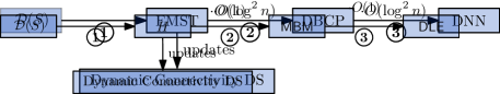
Figure 1: A solution with $O(\log^{10}n)$ update time.

Using Theorem 2.3, among other, as a subroutine, Chan et al. [10] developed a data structure for dynamic unit disk graphs with an update time of $O(\log^{10}n)$ and $O(\frac{\log n}{\log\log n})$ query time. As we use a similar framework in Section 3, we will briefly sketch their approach here. The construction is as follows (see Figure 1): let $T$ be the Euclidean minimum spanning tree (EMST) of $S$. If we remove all edges with length larger than $2$ from $T$, the resulting forest $F$ is a spanning forest for $\mathcal{D}(S)$. Thus, to maintain the components of $\mathcal{D}(S)$, it suffices to maintain the components of $F$. We create data structure $\mathcal{H}$ of Holm et al. to maintain $F$. Since the EMST has maximum degree $6$, inserting or deleting a site from $S$ changes $O(1)$ edges in $T$. Suppose we can efficiently find the set $E$ of edges that change during an update. Then, we can update the components in $F$ through $O(1)$ updates in $\mathcal{H}$, taking all edges in $E$ of length at most $1$. To find $E$, we need to dynamically maintain the EMST $T$ when $S$ changes. This can be done using a technique of Agarwal et al. that reduces the problem to several instances of the dynamic bichromatic closest pair problem (DBCP), with an overhead of $O(\log^{2}n)$ in the update time [3]. Eppstein showed that the DBCP problem can in turn be solved through a reduction to several instances of the dynamic nearest neighbor problem (DNN) for points in the plane [13]. Again, we incur another $O(\log^{2}n)$ factor as overhead in the update time. Using Chan’s DNN structure [9] with amortized expected update time $O(\log^{6}n)$, we get a total update time of $O(\log^{10}n)$. We can use $\mathcal{H}$ to answer queries in $O(\frac{\log n}{\log\log n})$ time.

(Compressed) Quadtrees and Cones

Let $\mathcal{G}_{i}$ be a grid with cell diameter $2^{i}$ and a grid point at the origin. The hierarchical grid $\mathcal{G}$ is then defined as $\mathcal{G}=\bigcup_{i=0}^{\lceil\log\operatorname{diam}(S)\rceil}\mathcal{G}_{i}$. For any cell $\sigma$ from the hierarchical grid, we denote by $|\sigma|$ its diameter and by $a(\sigma)$ its center. We call $i$ the level of the grid $\mathcal{G}_{i}$. Note that by the assumptions on $S$ this definition implies that $S$ is completely contained in a single cell of the highest level. Furthermore, for a given cell $\sigma\in\mathcal{G}_{i}$ and odd $k$, we call the $k\times k$ subgrid of $\mathcal{G}_{i}$ centered at $\sigma$ its $k\times k$ neighborhood and denote it by $N_{k\times k}(\sigma)$. See Figure 2 for a depiction of these concepts.

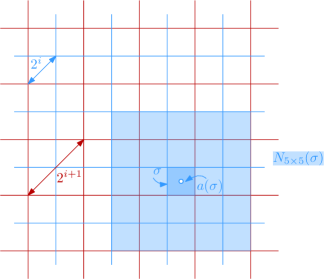
Figure 2: Two levels of the hierarchical grid.

The quadtree $\mathcal{T}$ on $S$ is a rooted tree whose nodes are a subset of cells from the hierarchical grid. The root is the cell with the smallest diameter that contains all sites of $S$. By our assumption on $S$, the root has diameter $\Theta(\operatorname{diam}(S))$. If a cell $\sigma$ with $|\sigma|=2^{i}$ for $i\geq 0$ contains at least two sites of $S$, then the children of $\sigma$ are the four cells $\tau$ with $|\tau|=2^{i-1}$ and $\tau\subseteq\sigma$. If a cell $\sigma$ contains only one site of $S$, it does not have any children. A quadtree on a given set of sites can be constructed in $O(n\log(\operatorname{diam}(S)))$ time [12]. In many cases, we will not explicitly distinguish between a cell $\sigma$ and its associated vertex in the quadtree.

For our applications in Section 4 and Section 6 we do not need the complete quadtree, but only a forest consisting of the lowest $k$ levels of a quadtree. Let $\mathcal{T}_{1},\dots\mathcal{T}_{l}$ be the quadtrees of the forest. In order to efficiently find the position of a cell or site in the quadforest, the cells associated with the root of each $\mathcal{T}_{i}$ are stored in a balanced binary search tree, lexicographically sorted by the coordinates of their lower left corners. This allows us to locate the quadtree containing the site or cell in $O(\log n)$ time. The position inside the quadtree can then be found in $O(k)$ additional time.

While the sites are stored in all cells of the quadtrees that contain them, we will associate each site with a fixed cell in the quadtree. This cell can intuitively be seen as an approximation of the site. We associate a site $s$ to the cell $\sigma_{s}$ of the quadtree, if:

1. $s\in\sigma_{s}$; and

2. $|\sigma_{s}|\leq s<2|\sigma_{s}|$.

If we define a quadtree as above, it has $O(n)$ leaves and height $O(\log(\operatorname{diam}(S)))$. This height does not depend on $n$ and can be arbitrary large. To avoid this, we define the compressed quadtree $\mathcal{Q}$. Let $\sigma_{1},\dots,\sigma_{k}$ be a maximal path in the full quadtree, where all $\sigma_{i}$, $1\leq i<k$, have only one non-empty child. In the compressed quadtree, this path is replaced by the single edge $\sigma_{1}\sigma_{k}$. Such a compressed quadtree has $O(n)$ vertices, height $O(n)$, and it can be constructed in $O(n\log n)$ time [7, 17]. Both for non-compressed and for compressed quadtrees we assume that we can compute the coordinates of the cell containing a site on a given level in $O(1)$ time.

Next, pick a constant $d\in\mathbb{N}$, and consider a set $\mathcal{C}_{d}$ of $d$ cones with their apex in the origin that cover the plane, each with opening angle $2\pi/d$. For some cell $\sigma\in\mathcal{T}$, we consider a copy $\mathcal{C}_{d}(\sigma)$ of this set of cones, with the common apex at $a(\sigma)$, as shown in Figure 3.

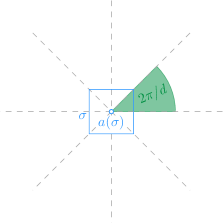
Figure 3: The cones $\mathcal{C}_{d}$ with angle $2\pi/d$ rooted at the center $a(\sigma)$ of a cell $\sigma$.

Heavy Path Decomposition

Let $T$ be a rooted ordered tree. An edge $uv\in T$ is called heavy if $v$ is the first child of $u$ in the given child-order that maximizes the total number of nodes in the subtree rooted at $v$ (among all children of $u$). Otherwise, the edge $uv$ is light. By definition, every internal node in $T$ has exactly one child that is connected by a heavy edge.

A heavy path is a maximum path in $T$ that consists only of heavy edges. The heavy path decomposition of $T$ is the set of all the heavy paths in $T$. The following lemma summarizes a classic result on the properties of heavy path decompositions.

Lemma 2.4 (Sleator and Tarjan [28]).

Let $T$ be a tree with $n$ vertices. Then, the following properties hold:

1. Every leaf-root path in $T$ contains $O(\log n)$ light edges;

2. every vertex of $T$ lies on exactly one heavy path; and

3. the heavy path decomposition of $T$ can be constructed in $O(n)$ time.

Dynamic Lower Envelopes in Two Dimensions

Let $L$ be a set of pseudolines in the plane, i.e., each element of $L$ is a simple continuous curve and any two distinct curves in $L$ intersect in exactly one point. The lower envelope of $L$ is the pointwise minimum of the graphs of the curves in $L$. In Section 3 we need to dynamically maintain the lower envelope of $L$. Overmars and van Leeuwen show how to maintain the lower envelope of a set of lines with update time $O(\log^{2}n)$ such that vertical ray shooting queries can be answered in $O(\log^{2}n)$ time [23]. These vertical ray shooting queries report the lowest line at a given vertical position. Chan improves this to $O(\log^{1+\varepsilon})$ for updates and queries [8]. Using the kinetic heap structure of Kaplan et al. [22] one can obtain $O(\log n\log\log n)$. Brodal and showed that the optimal bound $O(\log n)$ can be achieved [6]. For pseudolines there is the following result due to Agrawal et al. [2]:

Lemma 2.5 (Agrawal et al. [2]).

Let $L$ be a dynamic set of at most $n$ pseudolines. We can maintain the lower envelope of $L$ with $O(\log^{2}n)$ amortized update time and $O(\log n)$ amortized query time.

Remark.

There is solid evidence [18] that the result of Kaplan et al. also carries over to the pseudoline setting, giving a better $O(n\log\log n)$ update time with an $O(\log n)$ query time, however there is no formal presentation of these arguments yet. The applicability of the result by Brodal and Jacob [6] is not clear to us, and poses an interesting challenge for further investigation.

Weighted Nearest Neighbor Data Structures

For efficiently implementing the connectivity data structures, we make use of additively nearest neighbor data structures (AWNN). Given a set of $n$ points $P\subseteq\mathbb{R}^{2}$, where each point is assigned a weight $w_{p}$, an AWNN when queried with a point $q\in\mathbb{R}^{2}$ reports the point $\arg\min_{p\in P}\|pq\|+w_{p}$. If the point set is static, that is no points are inserted or deleted, an additively weighted Voronoi diagram can be used. In such a Voronoi diagram the region of a point $p$ contains all $q\in\mathbb{R}^{2}$ for which the nearest neighbor query above reports $q$. The regions are bounded by hyperbolic and straight segments. Furthermore, the Voronoi region assigned to a single point is either convex or star shaped, that is the line segment from $p$ to any point on the boundary of its Voronoi cell does not intersect any other cells [26]. It can be constructed in $O(n\log n)$ time [15] and the nearest neighbor of a given query point can be found in $O(\log n)$ time by using a vertical strip decomposition of the Voronoi diagram [12]. For easier referencing, we summarize these considerations in the following lemma:

Lemma 2.6 ([12, 15, 26]).

There is a static AWNN which for a set $P\subseteq\mathbb{R}^{2}$ of $n$ points has $O(n\log n)$ preprocessing time and $O(\log n)$ query time.

The situation becomes a bit more complicated, if we allow the insertion and deletion of points from the data structure in addition to the nearest neighbor queries. This can be achieved by using a data structure by Kaplan et al. [21], that allows to dynamically maintain the lower envelope of certain surfaces while allowing for vertical ray shooting queries. The weighted distance function used in the AWNN satisfies the conditions needed to use their data structure. Combining Theorem 8.3 of Kaplan et al. [21] with an observation on the properties of the specific distance function considered here [21, Section 9] gives the following Lemma:

Lemma 2.7 (Kaplan et al. [21, Theorem 8.3, Section 9]).

There is a fully dynamic AWNN data structure that allows insertions in $O(\lambda_{6}(\log n)\log^{5}n)$ amortized expected time and deletions in $O(\lambda_{6}(\log n)\log^{9}n)$ amortized expected time. Furthermore, queries can be performed in $O(\log^{2}n)$ worst case time. The data structure requires $O(n\log^{3}n)$ space in expectation. $\lambda_{s}(n)$ is the maximum length of a Davenport-Schinzel sequence of order $s$ on $n$ symbols.

The maximum length of a Davenport-Schinzel sequence $\lambda_{s}(n)$ is almost linear in $n$ for a fixed $s$. For example, $\lambda_{6}(n)=n\cdot 2^{\Theta(\alpha^{2}(n))}$, where $\alpha(n)$ is the inverse Ackermann function [27, Section 3].

A Deeper Dive into Kaplan et al.

The main results of Kaplan et al. [21] are two data structures for lower envelopes, supporting vertical ray shooting queries in each of them. The data structures maintain a dynamic set of hyperplanes [21, Section 7] or continuous bivariate functions of constant description complexity [21, Section 8] in $\mathbb{R}^{3}$ under insertions and deletions. The second variant, which is used in Lemma 2.7 above, is an extension of the first, and the first is a slight extension of a data structure by Chan [9].

In Section 5 we modify the data structures by Kaplan et al. to additionally allow sampling a random element not above a given input point. Here, we will briefly describe the data structures and introduce some notation, so we can build upon it later. The notation used here is consistent with the notation used by Kaplan et al. in their work.

The data structures use vertical $k$-shallow $(1/r)$-cuttings as their most integral part. Let $\mathcal{A}(H)$ be the arrangement of a set of hyperplanes $H$ in $\mathbb{R}^{3}$. The $k$-level $L_{k}$ of $\mathcal{A}(H)$ is the closure of all points of $\bigcup_{h\in H}h$ with $k$ hyperplanes of $H$ strictly below it. Then, $L_{\leq k}(H)$ (or $L_{\leq k}$ if the set of hyperplanes is clear from the context) is the union of the levels not above $L_{k}$. A vertical $k$-shallow (1/r)-cutting is a set $\Lambda$ of pairwise openly disjoint prisms, such that the union of $\Lambda$ covers $L_{\leq k}$, the interior of each $\tau\in\Lambda$ is intersected by at most $|H|/r$ hyperplanes of $H$, and each prism is vertical (i.e. it consists of a triangle and all points below it). Some or all vertices of a prism’s ceiling may lie at infinity. We define the size of the cutting to be the number of prisms. Using the algorithm by Chan and Tsakalidis a vertical $\Theta(|H|/r)$-shallow $1/r$-cutting of size $O(r)$ can be created in $O(|H|\log r)$ time [11]. The conflict list $\operatorname{CL}(\tau)$ of a prism $\tau$ is the set of all hyperplanes crossing its interior.

This notion can also be extended to bivariate functions. Then the regions are vertical pseudo-prisms, where the ceiling is limited by a pseudo-trapezoid part of a function [21, Section 3].

The data structure of Kaplan et al. for hyperplanes consists of $O(\log n)$ static substructures of exponentially decreasing size, where $n$ is the current number of hyperplanes. Substructures are periodically rebuilt similar to the Bentley-Saxe technique [4], and the whole data structure is rebuild after $\Theta(n)$ updates.

Each substructure of $n^{\prime}$ elements consists of a hierarchy of $m+2$ vertical shallow cuttings ${\{\Lambda_{j}\}}_{0\leq j\leq m+1}$ with $m\in O(\log n^{\prime})$, each with an associated set $H_{j}$ of hyperplanes. We set $k_{j}=2^{j}k_{0}$ where $k_{0}$ is a constant. Furthermore, let $n_{j}=|H_{j}|$ be the number of planes in $\Lambda_{j+1}$ and let $\alpha$ be a constant. $\Lambda_{m+1}$ consists of a single prism covering all of $\mathbb{R}^{3}$. The cutting $\Lambda_{j}$ for $j<m+1$ consists of a vertical $k_{j}$-shallow $(\alpha k_{j}/n_{j})$-cutting of the hyperplanes of $\Lambda_{j+1}$. The set $H_{j}$ contains all hyperplanes of $H_{j+1}$ that do not intersect too many prisms. Thus, the prisms of $\Lambda_{j}$ cover $L_{\leq k_{j}}(H_{j+1})$ and each conflict list contains at most $\alpha k_{j}$ hyperplanes. A substructure requires $O(n^{\prime}\log n^{\prime})$ space and building it requires $O(n^{\prime}\log^{2}n^{\prime})$ time.

The substructures are defined iteratively as follows. For the first substructure, we have $H_{m+1}=H$ and we collect the set $H^{\prime}=H_{m+1}\setminus H_{0}$ of hyperplanes. The procedure is then repeated for the next substructure, using $H^{\prime}$ as the initial set of hyperplanes, until $H^{\prime}$ is empty. This guarantees that each hyperplane is in the set $H_{0}$ associated to the shallow cutting $\Lambda_{0}$ for at least one substructure.

Vertical ray shooting queries are done by searching the shallow cuttings $\Lambda_{0}$ of all $O(\log n)$ substructures for the prism intersecting the vertical line containing the given position in $O(\log n)$ time each. Then, all obtained prisms are searched for the lowest plane along the line in $O(\log n)$ time.

Insertions are handled with a Bentley-Saxe approach that is, we rebuild multiple smaller substructures into new substructures periodically. The insertions require $O(\log^{3}n)$ amortized time.

Deletions are handled differently. In all substructures, hyperplanes are only marked as deleted and ignored in queries. As described above, queries are only performed in the shallow cuttings $\Lambda_{0}$ of each substructure. Thus, the lowest non-deleted hyperplane along a given vertical line might not be contained in the prism of $\Lambda_{0}$ intersecting said line. It may require the corresponding prism of $\Lambda_{1}$ or an even higher $\Lambda_{j}$, as prisms from higher cuttings can intersect more hyperplanes.

To handle this problem, when deleting a hyperplane $h$ in a substructure, all prisms containing $h$ are identified. For each such prism an individual counter is incremented. If this counter reaches a fraction of $f=\tfrac{1}{2\alpha{}}$ of the size of its conflict list, the prism and its hyperplanes are marked as purged in the substructure. When hyperplanes are first marked as purged in a substructure, they are also reinserted into the data structure. Hyperplanes marked as purged in a substructure are skipped in queries as well.

Consider the prisms $\tau_{1}$, …, $\tau_{m+1}$ from $\Lambda_{1}$, …, $\Lambda_{m+1}$ intersecting a vertical line. The idea behind the purging is that we have $|\operatorname{CL}(\tau_{j})|\leq\alpha k_{j}$ and $\Lambda_{j-1}$ covers $L_{\leq k_{j-1}}$ of the hyperplanes of $\Lambda_{j}$ due to the way the cuttings got constructed. See Figure 11 for a visualization. Thus, a fraction of at least $\tfrac{k_{j-1}}{\alpha k_{j}}=\tfrac{1}{2\alpha}=f$ hyperplanes of $\operatorname{CL}(\tau_{j})$ is intersected by $\tau_{j-1}$. A hyperplane first appearing in $\operatorname{CL}(\tau_{j})$ then can only be the lowest along the vertical line if all hyperplanes from $\operatorname{CL}(\tau_{j-1})$, and thus also a fraction of $f$ of the hyperplanes in $\operatorname{CL}(\tau_{j})$ have been deleted. Then, $\tau_{j}$ would have been purged and its hyperplanes reinserted into other substructures. Also, each hyperplane is contained in at most one substructure in $\Lambda_{0}$ without being marked as purged or deleted. Hence, a non-deleted hyperplane is contained in exactly one substructure in $\Lambda_{0}$ without being marked as purged.

Deletions require $O(\log^{5}n)$ amortized time and overall $O(n\log n)$ space is needed.

In addition to the lower envelope data structure for hyperplanes, Kaplan et al. describe how to create shallow cuttings of totally defined continuous functions $\mathbb{R}^{2}\to\mathbb{R}$ of constant description complexity [21, Theorem 8.1, Theorem 8.2]. Afterwards, they use it as a black box in their hyperplane data structure to yield the data structure for continuous bivariate functions of constant description complexity [21, Theorem 8.3, Theorem 8.4]. The analysis is similar to the one sketched above, however some parameters are chosen differently. When all subsets of the functions form a lower envelope of linear complexity, then the data structure allows insertions in $O(\lambda_{s}(\log n)\log^{5}n)$ amortized expected time, deletions in $O(\lambda_{s}(\log n)\log^{9}n)$ amortized expected time, and each query requires $O(\log n^{2})$ time. The data structure requires $O(n\log^{3}n)$ storage in expectation. $\lambda_{s}(n)$ is the maximum length of a Davenport-Schinzel sequence of order $s$ on $n$ symbols [27] and its value $s$ depends on the functions.

3 Unit Disk Graphs

In this section we describe a data structure for the fully dynamic connectivity problem on unit disk graphs. The idea is similar to the data structure by Chan et al. described in Section 2. However, we replace the Euclidean minimum spanning tree by a simpler graph that still captures the connectivity. We also replace the dynamic nearest neighbor data structure by a suitable dynamic lower envelope DLE structure. Both these improvements allow our data structure to gain a significant improvement to $O\mathopen{}\mathclose{{}\left(\log^{2}n}\right)$ amortized update time, without affecting the query time. The overall structure of our data structure is is shown in Figure 4.

Figure 4: The structure for our data structure

We define a proxy graph $H$ that represents the connectivity of $\mathcal{D}(S)$. The vertices of $H$ are cells of a grid. To see if two grid cells are connected by an edge, we maintain a bichromatic matching of the sites in the grid cells. This matching is updated with the help of two DLE data structures.

We start by formally defining the proxy graph. For this we consider the grid $\mathcal{G}_{1}$ of cells with diameter $2$. For $S\subset\mathbb{R}^{2}$, we define a graph $H$ whose vertices are the non-empty cells $\sigma\in\mathcal{G}_{1}$, i.e., the cells with $\sigma\cap S\neq\emptyset$. We say that $\sigma$ and $\tau$ are neighboring cells, if $\sigma\in N_{5\times 5}(\tau)$ and $\tau\in N_{5\times 5}(\sigma)$. Two cells $\sigma$ and $\tau$ are connected by an edge in $H$, if there is an edge $\{s,t\}\in\mathcal{D}(S)$ with $s\in\sigma$ and $t\in\tau$. We say that $s$ is assigned to the cell $\sigma$ containing it. The following lemma shows that the graph $H$ defined this way is sparse and accurately represents the connectivity in $\mathcal{D}(S)$.

Lemma 3.1.

The graph $H$ as defined above has $O(n)$ vertices, each with degree $O(1)$. Let $s,t\in S$ be two sites. Then $s$ and $t$ are connected in $\mathcal{D}(S)$, if and only if the cells $\sigma$ and $\tau$ that $s$ and $t$ are assigned to respectively are connected in $H$.

Proof 3.2.

To bound the size, observe that only cells containing at least one site are added to $H$, thus the number of vertices is $O(n)$. Furthermore, a cell $\sigma$ can only be connected to the $O(1)$ cells in $N_{5\times 5}(\sigma)$, as the distance to all cells outside this neighborhood is larger than $2$.

To show the claim about the connectivity, note that all sites that lie in the same cell $\sigma$ induce a clique in $\mathcal{D}(S)$. This follows as $\|ss^{\prime}\|\leq|\sigma|=2$ for all sites $s,s^{\prime}\in\sigma$. If two sites are connected by a path in $\mathcal{D}(S)$, it suffices to show that every single edge of the path connecting them is represented in $H$. Let $s,t$ be an edge in $\mathcal{D}(S)$. Then there are cells $\sigma$ and $\tau$ with $s\in\sigma$ and $t\in\tau$. As the edge $s,t$ exists in $\mathcal{D}(S)$, the edge $\{\sigma,\tau\}$ also exists in $H$ and we are done. For the other direction, it suffices to show that if there is an edge $\{\sigma,\tau\}\in H$ then all sites assigned to $\sigma$ are connected to all sites assigned to $\tau$ with a path in $\mathcal{D}(S)$. As the edge $\{\sigma,\tau\}$ exists in $H$ there is at least one pair $s,t$ of sites with $s\in\sigma,t\in\tau$ and $\|st\|\leq 2$. Then all sites in $\sigma$ are connected to $s$ via the clique in $\mathcal{D}(S)$ and all sites in $\tau$ are connected to $t$. The claim about the connectivity follows.

We build a data structure $\mathcal{H}$ as given in Theorem 2.3 for $H$. When querying the connectivity between sites $s$ and $t$, we first identify the cells $\sigma$ and $\tau$ in $\mathcal{G}_{1}$ assigned to the sites. The query is then performed on $\mathcal{H}$, using $\sigma$ and $\tau$ as the query vertices. When a site $s$ is inserted into or deleted from $S$, only the edges incident to the cell $\sigma$ containing it are affected. By Lemma 3.1, there are only $O(1)$ such edges. Thus, once the set $E$ of changing edges is determined, by Theorem 2.3 we can update $\mathcal{H}$ in time $O\mathopen{}\mathclose{{}\left(\log^{2}n}\right)$.

Finding the Edges $E$.

It remains to find the edges $E$ of $H$ that change when we update $S$. For this, we maintain for each pair of non-empty neighboring cells a maximal bichromatic matching (MBM) between their sites, similar to Eppstein’s method [13]. Let $R\subseteq S$ and $P\subseteq S$ be two disjoint site sets and let $(R\times P)\cap\mathcal{D}(S)$ be the bipartite graph on $R\mathop{\dot{\cup}}P$, consisting of all edges of $\mathcal{D}(S)$ with one vertex in $R$ and one in $P$. An MBM between $R$ and $P$ is a maximal set of vertex-disjoint edges in $(R\times P)\cap\mathcal{D}(S)$.

For each pair $\{\sigma,\tau\}$ of neighboring cells in $\mathcal{G}_{1}$, we build an MBM $M_{\{\sigma,\tau\}}$ for $R=\sigma\cap S$ and $P=\tau\cap S$. By definition, there is an edge between $\sigma$ and $\tau$ in $H$ if and only if $M_{\{\sigma,\tau\}}$ is not empty. When inserting or deleting a site $s$ from $S$, we proceed as follows: let $\sigma\in\mathcal{G}_{1}$ be the cell associated to $\sigma$. We go through all cells $\tau\in N_{5\times 5}(\sigma)$ and update $M_{\{\sigma,\tau\}}$ by inserting or deleting $s$ from the relevant set. If $M_{\{\sigma,\tau\}}$ becomes non-empty during an insertion or becomes empty during a deletion, we add the edge $\{\sigma,\tau\}$ to $E$ and mark it for insertion or deletion, respectively. We summarize this construction in the following lemma.

Lemma 3.3.

Suppose we can maintain an MBM for each pair of non-empty neighboring cells with update time $O(U(n))$, where $n$ is the maximum number of sites. Then we can dynamically maintain the adjacency lists of $H$ with update time $O(U(n))$.

Dynamically Maintaining an MBM.

Let $\sigma\neq\tau$ be two neighboring cells of $\mathcal{G}_{1}$, and let $P=\sigma\cap S$ and $B=\tau\cap S$. We show that an MBM between $P$ and $B$. can be efficiently maintained using two DLE structures for pseudolines. We fix a line $\ell$ that separates $P$ and $B$. Since $P$ and $B$ are in two distinct grid cells, we can take a supporting line of one of the four boundaries of $\sigma$. We have the following lemma.

Lemma 3.4.

Let $P,B\subseteq S$ be two sets with a total of at most $n$ sites, separated by a line $\ell$. There exists a dynamic data structure that maintains an MBM for $P$ and $B$ with $O(\log^{2}n)$ update time.

Proof 3.5.

We rotate and translate everything such that $\ell$ is the $x$-axis and all sites in $P$ have positive $x$-coordinate. We consider the set $U_{P}$ of disks with radius $2$ and their centers in $P$ (see Figure 5). Note that this is twice the radius of the unit disks. Then a site in $B$ forms an edge with some site in $P$ if and only if it is contained in the union of the disks in $U_{P}$. To detect this, we maintain the lower envelope of $U_{P}$. More precisely, consider the following set $L_{P}$ of pseudolines: for each disk of $U_{P}$, take the arc that defines the lower part of the boundary of the disk and extend both ends straight upward to $\infty$.

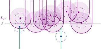
Figure 5: The set $L_{P}$ induced by $P$. The unit disks are drawn dashed. If a site $b\in B$ lies above the lower envelope, the unit disks intersect.

We build a data structure $D_{P}$ for $L_{P}$ according to Lemma 2.5. Analogously, we define a set of pseudolines $L_{B}$ and a dynamic envelope structure $D_{B}$ for $B$.

To maintain the MBM $M$, we store in $D_{P}$ the currently unmatched sites of $P$, and in $D_{B}$ the currently unmatched sites of $B$. When inserting a site $b$ into $B$, we perform a vertical ray shooting query in $D_{B}$ from $-\infty$ at the $x$-coordinate of $b$ to get a pseudoline of $L_{P}$. Let $p\in P$ be the site for that pseudoline. If $\|bp\|\leq 2$, we add the edge $\{b,p\}$ to $M$, and delete the pseudoline of $p$ from $D_{P}$. Otherwise we insert the pseudoline of $b$ into $D_{B}$. By construction, if there is an edge between $b$ and an unmatched site in $P$, then there is also an edge between $b$ and $p$. Hence, the insertion procedure correctly maintains an MBM. Now suppose that we want to delete a site $b$ from $B$. If $b$ is unmatched, we delete the pseudoline corresponding to $b$ from $D_{B}$. Otherwise, we remove the edge $\{b,p\}$ from $M$, and we reinsert $p$ as above, looking for a new unmatched site in $B$ for $p$. Updating $P$ is analogous.

Inserting and deleting a site requires $O(1)$ insertions, deletions, or queries in $D_{P}$ or $D_{B}$, so the lemma follows.

We obtain the main result of this section:

Theorem 3.6.

There is a dynamic connectivity structure for unit disk graphs such that the insertion or deletion of a site takes amortized time $O\mathopen{}\mathclose{{}\left(\log^{2}n}\right)$ and a connectivity query takes worst-case time $O(\frac{\log n}{\log\log n})$, where $n$ is the maximum number of sites at any time. The data structure requires $O(n)$ space.

Proof 3.7.

The main part of the theorem follows from a straightforward combination of Lemmas 3.1, LABEL:, 3.4 and 3.3. For the space bound, note that the MBMs have size linear in their involved sites and every site is contained in a constant number of cells and MBMs. Also, the number of overall edges is linear in $n$ and thus the data structure by Holm et al. requires linear space as well.

4 Polynomial dependence on $\Psi$

Naturally, the dynamic connectivity of disk graphs can be seen as an extension of the dynamic connectivity of unit disk graphs. This leads to similar approaches and data structures, although the size differences introduce new issues.

Initially, we will adapt the data structure from Theorem 3.6 to handle disks of different sizes. Instead of a single grid with fixed diameter this data structure will rely on a hierarchical grid, where sites are assigned to levels according to their radius. Due to the different radii the maximal bichromatic matchings are more complex to maintain, increasing the cost per cell pair. Additionally, a disk can now intersect disks from a significant larger number of other cells.

To overcome the last drawback at least partially, in Section 4.2 we will handle cells whose assigned disks are surely contained in an updated disk differently. This requires a more complicated query approach, which is introduced in Section 4.3 and increases its cost slightly by a factor of $O(\log\log n)$.

Note that the approach in Section 4.1 follows a similar approach as presented by Kaplan et al. [21, Theorem 9.11] which achieves the same time and space bounds. The details of our implementation are however crucial for the adaptations in Sections 4.2 and 4.3. Notably, our implementation uses a hierarchical grid instead of a single fine grid.

4.1 Adapting the Unit Disk Case

Recall that we defined the hierarchical grid $\mathcal{G}$ to contain the cells of levels $0$ to $\lceil\log\operatorname{diam}(S)\rceil$. Each site $s\in S$ is assigned to the corresponding cell $\sigma_{s}\in\mathcal{G}$ with $s\in\sigma_{s}$ and $|\sigma_{s}|\leq r_{s}<2|\sigma_{s}|$. Note that this is in contrast to the data structure of Section 3, where all sites with radius $1$ are assigned to cells with diameter $2$. We will denote the sites assigned to a cell $\sigma$ by $S(\sigma)$ and call $\log|\sigma_{s}|$ the level of the site $s$. We only consider cells that have at least one site assigned to them. Hence, only the lowest $\lfloor\log\Psi\rfloor+1$ levels of $\mathcal{G}$ will be used. Again, all sites assigned to the same cell form a clique.

As for the unit disk graphs, we define a proxy graph $H$ based on the grid and intersecting disks. The vertices of $H$ are the cells of $\mathcal{G}$ that have at least one assigned site. We connect two cells $\sigma,\tau\in\mathcal{G}$ by an edge if and only if we have $\{s,t\}\in\mathcal{D}(S)$ for some $s\in S(\sigma)$ and $t\in S(\tau)$. Note that $\sigma$ and $\tau$ do not have to be on the same level of the hierarchical grid. Generally, we call a pair of cells $\sigma$, $\tau$ neighboring if and only if it is possible that some assigned disks between them could intersect, i.e. their distance is less than $2|\sigma|+2|\tau|$, see Figure 6. Unfortunately, a cell can have a lot more edges compared to the unit disk case as made clear in the following lemma.

Lemma 4.1.

The graph $H$ as defined above has $O(n)$ vertices, each with degree $O(\Psi^{2})$. Let $s,t\in S$ be two sites. Then $s$ and $t$ are connected in $\mathcal{D}(S)$ if and only if the cells $\sigma$ and $\tau$ with $s\in\sigma$ and $t\in\tau$ are connected in $H$.

Proof 4.2.

The number of vertices directly follows from the fact that only cells with an assigned site are used as vertices.

To bound the degree, recall that all sites are assigned to the lowest $\lfloor\log\Psi\rfloor+1$ levels only. Fix any cell $\sigma\in G_{\ell}$ with $\ell\in[0,\lfloor\log\Psi\rfloor]$. The neighborhood on the same level $\ell$ of $\sigma$ is completely contained in $N_{13\times 13}(\sigma)$. Now let $\sigma^{\prime}$ be the cell containing $\sigma$ in a level above $\ell$. Then all neighboring cells of $\sigma$ lie in $N_{13\times 13}(\sigma^{\prime})$. For the levels below $\ell$, note that no cell that is not contained in $N_{13\times 13}(\sigma)$ can be neighboring to $\sigma$. Altogether, the number of neighboring cells, and thus the degree, is at most

$$13^{2}\cdot\sum_{i=0}^{\lfloor\log\Psi\rfloor}{(2^{i})}^{2}\in O(\Psi^{2})$$

per cell. Note that this bound is asymptotically tight, as all cells of the hierarchical grid that are contained in $\sigma_{s}$ are neighboring to $\sigma$. The connectivity follows analogous to the proof of Lemma 3.1.

Figure 6: The neighborhood of the red colored cell in $\mathcal{G}_{i-1}$. The area of the neighboring cells in one level beneath is colored in a darker shade.

Consider the lowest $\lfloor\log\Psi\rfloor+1$ levels of the quadtree containing $S$. We can store the roots of these quadtrees in a binary search tree as described in Section 2. This allows us to locate any cell of these lowest $\lfloor\log\Psi\rfloor+1$ levels in $O(\log n+\log\Psi)$ time. We can insert a new cell on level $\lfloor\log\Psi\rfloor+1$ in $O(\log n)$ time.

We augment the quadtrees with additional information and cells. To be precise, for each site $s\in S$ we make sure to that cells in $N_{13\times 13}(\sigma_{s})$ are contained in the quadforest. As these are only $O(1)$ cells they can be updated in $O(\log n+\log\Psi)$ time on the insertion or deletion of $s$ and adding them does not change the asymptotic time and space bounds for the quadtree structure. We also add pointers between adjacent cells on the same levels. These pointers can be maintained in a similar fashion to the maintenance of the cells in the $13\times 13$ neighborhoods. We call the resulting structure $\mathcal{T}$ and assume that at the insertion or deletion of a site or cell the additional information is updated accordingly.

Similarly to the unit disk case, our (intermediate) goal is to fully represent and update the proxy graph $H$ using an instance $\mathcal{H}$ of the data structure due to Holm et al., see Theorem 2.3. Then, we can use $\mathcal{T}$ and $\mathcal{H}$ to query for connectivity given two sites $s$, $t$. To do so, the cells $\sigma$ and $\tau$, that have $s$ and $t$ assigned, are obtained. Afterwards, $\mathcal{H}$ is queried for $\sigma$ and $\tau$, which yields the correct result according to Lemma 4.1.

Inserting or deleting a site works similar as in the unit disk case as well, but the different radii complicate things a bit. We have to obtain the $O(\Psi^{2})$ updated edges and update $\mathcal{H}$ for each changed edge. Again, we find these edges via maintaining a maximum bichromatic matching (MBM) for each pair of neighboring cells and their associated sites. When inserting or deleting a site in a cell $\sigma$, all MBM between $\sigma$ and its neighbors are updated. Following the definitions of $H$ and the MBM, the graph $H$ contains an edge between two cells if and only if their MBM is not empty. Hence, if an update to an MBM matches a first edge or deletes a last edge, $\mathcal{H}$ is updated accordingly. Due to the different radii we have to resort to a more involved data structure for the MBM, but the overall approach is based on the same simple idea as in the unit disk case.

Dynamically Maintaining an MBM.

Let $\sigma\neq\tau$ be two neighboring cells of $\mathcal{G}$, and let $P=\sigma\cap S$ and $B=\tau\cap S$. We show that an MBM between $P$ and $B$ can be efficiently maintained using two fully dynamic AWNN structures using the following lemma.

Lemma 4.3 (Kaplan et al. [21, Lemma 9.10]).

Let $P,B\subseteq S$ be two sets with a total of at most $n$ sites. There exists a dynamic data structure that maintains an MBM for $P$ and $B$ with $O(\lambda_{6}\log^{9}n)$ expected amortized update time using $O(n\log^{3}n)$ expected space.

Proof 4.4.

A site $p\in P$ has an edge to a site $b\in B$ in $\mathcal{D(S)}$ if and only if we have $\|bp\|\leq r_{b}+r_{p}$. Given $p\in P$ we can obtain some $b\in B$ such $b$ intersects $p$ by maintaining a fully dynamic AWNN $D_{B}$ on the sites of $B$ with their negative radius as weight. Querying this data structure with $p$ returns the site $b\in B$ that induces the closest disk to $p\in P$ with its associated radius. If there exists a $b\in B$ fulfilling the requirement above, then the requirement is also fulfilled by the returned element, as it minimizes $\|bp\|-r_{b}$ with a fixed $r_{p}$.

Using this idea with the AWNN data structure of Lemma 2.7, yields the MBM data structure with the same approach as in the proof of Lemma 3.4. We maintain two AWNN data structures $D_{P}$ and $D_{B}$ for unmatched sites from $P$ and $B$, respectively. When inserting a new site, say, $p$ into $P$ we perform a nearest neighbor query in $D_{B}$ with it. In case some site $b\in B$ is returned and we have $\|bp\|\leq r_{b}+r_{p}$, then we add the edge $\{p,b\}$ to the matching and remove $b$ from $D_{B}$. Otherwise, we add $p$ with $r_{p}$ into $D_{P}$.

When deleting a site incident to an edge of the matching, we remove the edge and reinsert the other site of the edge as described above. Due to the observation above, every newly unmatched site either gets matched directly if possible or cannot get matched. Hence, this approach maintains the MBM.

Combining the knowledge and the descriptions above, we are able to show the following theorem.

Theorem 4.5.

There is a dynamic connectivity structure for disk graphs such that the insertion or deletion of a site takes amortized expected time $O(\Psi^{2}\lambda_{6}(\log n)\log^{9}n)$ and a connectivity query takes worst-case time $O(\frac{\log n}{\log\log n})$, where $n$ is the maximum number of sites at any time. The data structure requires $O(\Psi^{2}n\log^{3}n)$ expected space.

4.2 Limit the Insertions into the MBM

The quadratic dependence on $\Psi$ in the update bound of Theorem 4.5 can be reduced from quadratic to linear with a little bit more work. In this section we will reduce the dependency on $n$ in the $\Psi^{2}$ term by skipping some MBM updates, before removing it completely in Section 4.3.

Observe, that the radius of a site $s\in S$ assigned to cell $\sigma_{s}$ is equal to or larger than the cell’s diameter. Hence, the disk $D_{s}$ contains $\sigma_{s}$ and also all descendants of $\sigma_{s}$ in the quadtree $\mathcal{T}$. The same holds for every other cell that is contained in $D_{s}$.

When a cell $\sigma$ is contained in an updated disk induced by $s\in S$, we can conclude that all sites assigned to $\sigma$ intersect the disk. Using this observation, we can often avoid updating the MBM. Instead, checking whether $\sigma$ has assigned sites and the MBM for emptiness is sufficient for updating the edge in the underlying connectivity structure in this case.

Unfortunately, this notion of contained cells is not strong enough for our approach to reduce the dependency on $\Psi$ in Section 4.3. There we require that a disk contains both a cell and all disks assigned to said cell.

Definition 4.6.

Let $D_{s}$ be a disk and $\sigma\in\mathcal{G}_{i}$ a cell, for some $i\geq 0$. Then, $\sigma$ is fully contained in $D_{s}$ if and only if $\sigma$ intersects $D_{s}$ and cannot have assigned disks that intersect the boundary of $D_{s}$. Additionally, $\sigma$ is topmost fully contained in $D_{s}$ if and only if there is no other cell $\tau$ fully contained in $D_{s}$ with $\sigma\subset\tau$.

The topmost fully contained cells are the first fully contained cell encountered on any path from the root of the quadforest $\mathcal{T}$.

Additionally, we bound the number of cells that still require updating an MBM after considering the fully contained cells. See Figure 7 for an example of the distribution of the different types of cells.

Figure 7: The types of cells which require checking when updating the black disk in the data structure of Theorem 4.5:    fully contained (topmost)   fully contained   may have disks intersecting the boundary

Lemma 4.7.

Inserting or deleting a site $s\in S$ of radius $r_{s}$ into the data structure of Theorem 4.5 requires checking $O(\Psi)$ cells that are not fully contained in the disk of $s$. Those can be found in $O(\Psi+\log n)$ time.

Proof 4.8.

First, we bound the number of cells on a single level, before concluding the first part of the lemma. The second part then follows almost immediately.

Let $\ell\leq\lfloor\log\Psi\rfloor$ be the level of $s$ and let $\sigma_{s}$ be the cell $s$ is assigned to. The cell $\sigma_{s}$ has only a constant number of neighboring cells on each level $j\geq\ell$. Hence, we focus on the levels smaller than $\ell$. Consider a grid $\mathcal{G}_{i}$ for some $i<\ell$. By the definition of the hierarchical grid, each cell in $\mathcal{G}_{i}$ has diameter $d=2^{i}$. The cells in $\mathcal{G}_{i}$ that are neighboring to $\sigma_{s}$ can be partitioned into three groups:

1. Cells that are contained in $D_{s}$, and cannot have an assigned disk that intersects the boundary of $D_{s}$,

2. cells that can have an assigned disk that intersects the boundary of $D_{s}$; and

3. cells that are not contained in $D_{s}$, and cannot have an assigned disk that intersects the boundary of $D_{s}$.

The last group are still neighbors of $\sigma_{s}$, as other disks of $\sigma_{s}$ could possibly intersect a disk of it. Still, we can skip them when updating $s$. As we want to bound the number of cells not fully contained in $D_{s}$, we need to bound the size of the second group only.

This group of cells consists of the cells of $\mathcal{G}_{i}$ that have a distance less than $2d$ from the boundary of $D_{s}$. Equivalently, they can be described as all cells intersecting the inner area of an annulus with inner radius $r_{s}-2d$ and outer radius $r_{s}+2d$ centered at $s$. We use the second interpretation to bound the size. For simplicity, we bound the number of all cells intersecting the annulus including its boundary.

Consider a rasterization of a circle as described by Bresenham [5]. This rasterization works by splitting the circle into eight equally sized octants and walking along the parts. Depending on the octant the movement of the rasterization is strictly monotone in one axis and there are always two adjacent octants that share their direction of strict monotonicity. A superset of all cells intersected by a given circle can be obtained by applying Bresenham’s algorithm and add at most one additional adjacent cell perpendicular to the strict monotone axis in each step. When generously rounding up the size of the four parts with different direction in their strict monotonicity, we can have at most $4\cdot 2\cdot(\lceil\frac{r_{s}-2d}{d/\sqrt{2}}+1\rceil+\lceil\frac{r_{s}+2d}{d/\sqrt{2}}+1\rceil)$ cells intersecting the two enclosing circles of the annulus, see Figure 8.

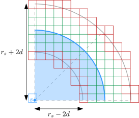
Figure 8: The red cells rasterize the two octants of the inner and outer annulus.

All remaining cells are contained in the annulus and have an overall area of at most $\pi(r_{s}+2d)^{2}-\pi(r_{s}-2d)^{2}$. Hence, we have at most

$$\mathopen{}\mathclose{{}\left\lfloor\frac{\pi(r_{s}+2d)^{2}-\pi(r_{s}-2d)^{2}}{d^{2}/2}}\right\rfloor=\mathopen{}\mathclose{{}\left\lfloor\frac{16\pi r_{s}}{d}}\right\rfloor$$

cells inside the annulus to consider.

We already noted that $s$ has only a constant number of neighbors in all levels larger than or equal to $\ell$. Hence, the worst case occurs when $s$ is of level $\lfloor\log\Psi\rfloor$. Conclusively, the number of cells over all grids which can contain disks intersecting the boundary of $s$ is at most

$$\phantom{{}\leq}\sum_{i=0}^{\lfloor\log\Psi\rfloor}4\cdot 2\cdot\mathopen{}\mathclose{{}\left(\mathopen{}\mathclose{{}\left\lceil\frac{r_{s}-2d}{d/\sqrt{2}}+1}\right\rceil+\mathopen{}\mathclose{{}\left\lceil\frac{r_{s}+2\cdot d}{d/\sqrt{2}}+1}\right\rceil}\right)+\mathopen{}\mathclose{{}\left\lfloor\frac{16\pi r_{s}}{d}}\right\rfloor$$

$$\leq\sum_{i=0}^{\lfloor\log\Psi\rfloor}4\cdot 2\cdot\mathopen{}\mathclose{{}\left(\frac{r_{s}-2d}{d/\sqrt{2}}+\frac{r_{s}+2d}{d/\sqrt{2}}+4}\right)+\frac{16\pi r_{s}}{d}$$

$$=\sum_{i=0}^{\lfloor\log\Psi\rfloor}4\cdot 2\cdot\mathopen{}\mathclose{{}\left(\frac{2r_{s}}{d/\sqrt{2}}+4}\right)+\frac{16\pi r_{s}}{d}$$

$$=16\sum_{i=0}^{\lfloor\log\Psi\rfloor}\frac{\sqrt{2}r_{s}+\pi r_{s}}{d}+2$$

$$=16\sum_{i=0}^{\lfloor\log\Psi\rfloor}\frac{(\sqrt{2}+\pi)r_{s}}{d}+2$$

$$=16\cdot\mathopen{}\mathclose{{}\left(2\mathopen{}\mathclose{{}\left(\mathopen{}\mathclose{{}\left\lfloor\log\Psi}\right\rfloor+1}\right)+\sum_{i=0}^{\lfloor\log\Psi\rfloor}\frac{(\sqrt{2}+\pi)r_{s}}{2^{i}}}\right)$$

$$\in O(\log\Psi+r_{s})\subseteq O(\Psi)$$

Every cell that can have an assigned disk $D_{t}$ such that $D_{t}$ intersects the boundary of $D_{s}$ must be the child of another cell with the same property or the root of a quadtree. Thus, these cells can be obtained by finding all such cells in layer $\ell$ and recursing down into the quadtrees. Finding the cells on layer $\ell$ can be done through the links between adjacent cells starting from $\sigma_{s}$ in constant time. Reaching layer $\ell$ itself takes time $O(\log\Psi+\log n)$ in the quadtree.

The cost for testing cells that do not intersect the circle can be charged to their parents, yielding the required time for obtaining every intersected cell.

Another look at the cells during the recursive retrieval yields the following corollary.

Corollary 4.9.

Updating the data structure from Theorem 4.5 requires checking $O(\Psi^{2})$ cells that are fully contained in $D_{s}$ on each insertion or deletion. These cells can be found in $O(\Psi^{2}+\log n)$ time.

Among all paths in the quadtrees there are $O(\Psi)$ topmost cells fully contained in $D_{s}$. These can be found in $O(\Psi+\log n)$ time. Their interiors are pairwise disjoint and their union is exactly the union of all cells fully contained in $D_{s}$.

Proof 4.10.

The number of cells follows directly from Lemma 4.1 and Lemma 4.7.

All cells that are fully contained in a disk are either the child of another fully contained cell or are a child of a cell that can have an assigned disk that intersects the boundary of the query disk. Hence, the retrieval described in Lemma 4.7 only needs to be extended such that it continues its recursion into fully contained cells.

As every fully contained cell has only other fully contained cells as children the union of the topmost among those cells is sufficient to cover the whole area of fully contained cells. Again, we can extend the recursion to retrieve all the topmost fully contained cells in the required time by looking at the quadtree roots and all children of considered not fully contained cells.

Using Corollary 4.9, we can save some time during updates: we do not update the MBM to fully contained cells, but insert an edge directly into the underlying edge connectivity structure if required.

Lemma 4.11.

There is a data structure for dynamic disk connectivity with expected amortized update time $O(\Psi^{2}\log^{2}n+\Psi\lambda_{6}(\log n)\log^{9}n)$ and worst case time $O(\tfrac{\log n}{\log\log n})$ for connectivity queries while requiring $O(\Psi n\log^{3}n+\Psi^{2}n)$ expected space.

Proof 4.12.

We augment the data structure of Theorem 4.5. In addition to an MBM, we save a counter for each neighboring pair of cells of different size. The counter describes how many of the disks of the larger cell fully contain the smaller cell.

When updating a pair during insertion or deletion of a site $s$, we now update either the counter or the MBM. If $D_{s}$ fully contains the other cell we update the counter, otherwise the MBM. Both cells’ content intersect if and only if the counter is non-zero and the smaller cell is non-empty or the MBM contains an edge. Depending on whether this condition changes during the update, the edge connectivity data structure must be updated as well.

When updating a disk $s$, we encounter $O(\log\Psi)$ neighboring cells until we reach the level where $s$ must be inserted or deleted. For each of these, an update to the MBM or the counter is required. Afterwards, we recurse down according to Corollary 4.9 to retrieve all $O(\Psi^{2})$ fully contained cells and the remaining $O(\Psi)$ cells described in Lemma 4.7 and update the MBMs, counters, and connectivity structure accordingly.

Due to the restrictions on the inserted cells and Lemma 4.7, there are at most $O(\min(n^{2},\Psi n))$ sites stored across all MBMs. Each MBM requires $O(n^{\prime}\log^{3}n^{\prime})$ storage in expectation, where $n^{\prime}$ is the number of sites stored in an MBM. The sum over all MBMs is thus maximized at a single MBM instance with $O(\Psi n\log^{3}n)$ expected space. The required space for the other elements is analogous to Theorem 4.5. In particular, the quadforest requires $O(\Psi^{2}n)$ space.

4.3 Query for Replacements Instead

We were able to reduce the factor of the quadratic part, but did not eliminate it. As we can have $O(\Psi^{2})$ edge changes in the proxy graph during an update in the previous approaches, we need to avoid handling all of them in the update. Instead, we continue handling fully contained cells and non-contained cells differently. To sidestep the costly edge updates for fully contained cells we move parts of the handling of fully contained cells to the query.

As the first step we show the following lemma, that allows us to ignore certain edges introduced by non-zero counters. Its general idea is illustrated in Figure 9(a).

Lemma 4.13.

Given two sites $s$ and $t$ and let $H^{\prime}$ be the subgraph of proxy graph $H$ that does not contain any fully contained cells, except for those associated with $s$ and $t$. Then, the cells associated to $s$ and $t$ are connected in $H^{\prime}$, if and only if $s$ and $t$ are connected in $\mathcal{D}(S)$.

Proof 4.14.

First, assume that $s$ and $t$ are not connected in $\mathcal{D}(S)$. As we do not add any edges, by Lemma 4.1 the cells associated to $s$ and $t$ are not connected in $H$, and thus also not in $H^{\prime}$. Thus, we assume in the following that $s$ and $t$ lie in the same connected component.

Let $\pi$ be a path connecting $s$ and $t$ in $\mathcal{D}(S)$. We show that this path can be iteratively changed to a path $\pi^{\prime}$ that connects $s$ and $t$ in $\mathcal{D}(S)$ and that is represented in $H^{\prime}$. As we are done when all edges in $\pi^{\prime}$ are in $H^{\prime}$, assume that the path uses at least one edge in $H\setminus H^{\prime}$ when the sites are mapped to cells.

Let $\{u,v\}$ be the first edge in $\pi$ that lies in $H\setminus H^{\prime}$ when mapped to cells. Without loss of generality, assume that $D_{u}$ fully contains $\sigma_{v}$. Here we can have two different cases: if $D_{u}$ also fully contains $\sigma_{t}$, we can replace $v$ and all following sites in the path by $t$. Otherwise, there exist at least one site $w$ somewhere after $v$ in $\pi$, such that $D_{u}$ does not fully contain $\sigma_{w}$ and $D_{u}$ and $D_{w}$ intersect. Note, that $w$ may be equal to $t$. The site $w$ has to exist, as $\sigma_{t}$ is not fully contained in $D_{u}$ and $D_{v}$ lies completely inside $D_{u}$. Also, $D_{t}$ either intersects $D_{u}$, or $D_{t}$ does not intersect $D_{u}$ so another disk $D_{w}$ must go through the boundary of $D_{u}$. In this case, the part in between $\pi$ and $w$ can be removed from $\pi$, yielding another connecting path with at least one edge less from $H\setminus H^{\prime}$ when mapped to cells.

(a) A path between the two red disks uses the black disks as intermediates. Note that any non-red disk contained by a black disk is not required to form a path and can be safely ignored.

(b) Removing the dashed disks and querying for $u$ instead of $s$ still leads to a valid path to $t$.

Figure 9: Depiction of the arguments in Lemma 4.13.

By Lemma 4.13 we can ignore fully contained cells during updates, as long as we make sure that the missing edges to the query sites are handled. To enable this, we maintain for each cell which disks fully contain them as topmost. Then, during a query we can sidestep the issue around the missing edges by querying for suitable representatives instead, which can be found via the maintained disks fully containing the cells. See Figure 9(b).

Lemma 4.15.

Given an instance of the data structure of Lemma 4.11 and two sites $s$ and $t$. Let $\sigma_{s^{\prime}}$ and $\sigma_{t^{\prime}}$ be the largest cells on the paths to $s$ and $t$ that are fully contained by some disks. Let $u$ and $v$ be the largest such disks for $\sigma_{s^{\prime}}$ and $\sigma_{t^{\prime}}$.

Then the cells associated to $u$ and $v$ are connected in the subgraph $H^{\prime}$ of the proxy graph $H$ that does not contain any cells that are fully contained in a disk of $S$ if and only if $s$ and $t$ are connected in $\mathcal{D}(S)$.

Proof 4.16.

We have already shown in Lemma 4.13 that omitting the cells in $H\setminus H^{\prime}$ except those associated to $s$ and $t$ does not change the connectivity between $s$ and $t$.

When $\sigma_{u}$ and $\sigma_{v}$ are connected in $H^{\prime}$, then $s$ and $t$ are obviously connected in $\mathcal{D}(S)$ by construction. For the other direction we use a similar idea as in the proof of Lemma 4.13 we described above. First, we will focus on replacing $s$ with $u$ in a path $\pi$ connecting $s$ and $t$ created by Lemma 4.13, such that the resulting path $\pi^{\prime}$ when mapped to cells only uses cells of $H^{\prime}$ except $t$. Afterwards, the same procedure can be repeated for $t$ and $v$ to completely create a path which, when mapped to its corresponding cells, uses cells from $H^{\prime}$ only.

Recall, that $D_{u}$ is the largest disk fully containing $\sigma_{s^{\prime}}$ on the path to $\sigma_{s}$. In particular, there is no disk fully containing $\sigma_{u}$. This doesn’t necessarily mean that $D_{u}$ is overall the largest disk fully containing $\sigma_{s}$. This warrants a small case distinction for replacing $s$ with $u$.

If $D_{u}$ is the largest disk fully containing $\sigma_{s}$, then we can directly apply the idea of the proof of Lemma 4.13, showing that $u$ and $t$ are connected through a path $\pi^{\prime}$ without using any site except $t$ belonging to an omitted cell. When $D_{u}$ is not the largest disk fully containing $\sigma_{s}$, then there must be a larger disk $D_{u^{\prime}}$ fully containing $\sigma_{s}$, on which the previous idea can be applied. As both disk fully contain $\sigma_{s}$, they intersect. Hence, $u$ is connected via $u^{\prime}$ to $t$ without using any site except $t$ belonging to an omitted cell.

Note, that in Lemma 4.15 it directly follows from Definition 4.6 that $\sigma_{s^{\prime}}$ is topmost fully contained by $D_{u}$. The same holds for $\sigma_{t^{\prime}}$ and $D_{v}$.

The dynamic nested rectangle intersection data structure by Kaplan et al. [20, Section 5] allows inserting or deleting nested or disjoint rectangles with a priority in $O(\log^{2}n)$ amortized time, and retrieving the highest priority rectangle containing a query point in amortized time $O(\log n)$, while requiring $O(n\log n)$ space. We can use it to retrieve the representatives without a dependency on $\Psi$ in the query time by storing all fully contained topmost cells. This allows us to apply the recent lemmas to the data structure of Lemma 4.11.

Theorem 4.17.

There is a data structure for dynamic disk connectivity with expected amortized update time $O(\Psi\lambda_{6}(\log n)\log^{9}n)$ and amortized time $O(\log n)$ for connectivity queries while requiring $O(\Psi n\log^{3}n)$ expected space.

Proof 4.18.

We augment the data structure of Theorem 4.5 similar to Lemma 4.11. Instead of a counter, we maintain for each cell a balanced binary search tree of all disks which topmost fully contain this cell, ordered by radius. Also, we maintain in each node of the quadforest the number of disks in its subtree.

Additionally, we maintain a rectangle intersection data structure as described by Kaplan et al. [20]. Each cell with a non-empty balanced binary search tree and a non-zero disk count in its subtree is inserted into the data structure with its size as priority. Due to the restriction on inserted cells and Corollary 4.9, there are at most $O(\min(n^{2},\Psi n))$ cells stored in the rectangular intersection data structure simultaneously. Similarly, due to Lemma 4.7 there are at most $O(\min(n^{2},\Psi n))$ sites stored across all MBMs.

During a disk update, we perform $O(\Psi)$ updates to the rectangle structure because of changes to the topmost fully contained cells, and $O(\log\Psi)$ updates along the path in the quadforest induced by changes to counters. As each of these updates requires $O(\log(n^{2}))=O(\log n)$ amortized time, and we have to update at most $\Psi$ MBMs, the overall update time is reduced by a factor of $\Psi$ in contrast to Theorem 4.5.

Queries are done by finding the representatives described in Lemma 4.15 with the help of the rectangle data structure and the balanced binary trees in $O(\log(n^{2})+\log n)=O(\log n)$ amortized time and then querying the connectivity structure as before.

We need $O(\min(n^{2},\Psi n)\log\min(n^{2},\Psi n))=O(\Psi n\log n)$ space for the rectangular intersection data structure. As in the proof of Lemma 4.11, we have $O(\min(n^{2},\Psi n))$ sites stored across all MBMs and each MBM requires $O(n^{\prime}\log^{3}n^{\prime})$ storage in expectation, where $n^{\prime}$ is the number of sites stored in an MBM. The sum over all MBMs is thus maximized at a single MBM instance with $O(\Psi n\log^{3}n)$ expected space. All sites are contained in $O(\Psi)$ binary search trees, hence the overall storage of these trees is $O(\Psi n)$. The number of nodes in the quadforest is also limited to $O(\Psi n)$, as every site can introduce at most $\Psi$ cells. Altogether, the space is dominated by the MBMs and the theorem follows.

5 Reveal Data Structure

Dynamic data structures for dynamic connectivity have two major obstacles to tackle for updating: A single update can change the connectivity graph severely, and it is often nontrivial how an update influences the underlying graph or a constructed proxy graph. Before we can continue in Section 6 to build data structures for semi-dynamic settings, which bring the dependence on $\Psi$ down to a logarithmic factor, we have to solve the second problem first. In particular, it is not obvious how to obtain all affected sites of a set in the deletion-only setting.

To be more precise, let $P$ and $B$ be two sets of disks in $\mathbb{R}^{3}$, such that for each disk $p\in P$ exists at least one disk $b\in B$ it intersects. We now want to remove a disk $b\in B$ and obtain all disks $p\in P$ that no longer intersect any disk in $B$. We call such disks revealed, see Figure 10.

Figure 10: When removing a blue disk, we want to obtain all purple disks intersecting this blue disk but no other blue disk. After removing the dashed blue disk, the dashed purple disks need to be obtained.

A data structure for detecting such revealed disks is constructed over the course of Sections 5.1 and 5.2, which conclude in Theorem 5.10. The central idea of the data structure is representing intersections sparsely by assigning each $p\in P$ repeatedly to one $b\in B$ intersecting $p$ until no such $b$ exists any more and $p$ is revealed. To avoid a problematic order of the assignments we perform these assignments randomly. That means we need to randomly sample a disk among all disks in $B$ that intersect a given disk $p\in P$.

Obtaining such a random disk that intersects a query disk out of a given semi-dynamic set is the main problem we work on in this section. We construct a data structure for solving this problem and build upon the dynamic lower envelope data structures by Kaplan et al., which we briefly discussed in Section 2. Similarly to the original construction by Kaplan et al., we will do this construction in two steps. First, a simpler data structure for sampling a disk containing a given point, which builds upon the data structure of Kaplan et al. for hyperplanes [21, Section 7] is constructed. Afterwards, the data structure of Kaplan et al. for continuous bivariate functions of constant description complexity [21, Section 8] is extended in the same way, resulting in a data structure for sampling a disk intersecting a given disk.

5.1 Sampling Hyperplanes

We begin by constructing a data structure for the simpler problem of sampling a random disk containing a given point from a dynamic set of disks. Using linearization [1, 30] we can transform this problem in $\mathbb{R}^{2}$ into the problem of sampling a hyperplane not above a given point in $\mathbb{R}^{3}$. This allows us to build upon the data structure for hyperplanes by Kaplan et al.

Recall from Section 2 that the data structure uses $O(\log n)$ substructures, which in turn use a logarithmic number of shallow cuttings $\Lambda_{j}$, each with an associated set $H_{j}$ of hyperplanes.

When deleting a hyperplane it will only be marked as such in the respective substructure. The central idea behind the data structure builds on the structure of the hierarchy of cuttings: the prisms of $\Lambda_{j-1}$ cover $L_{\leq k_{j-1}}(H_{j})$ and each of their conflict lists contains at most $\alpha k_{j-1}$ hyperplanes. This implies, that for each $\tau_{j-1}\in\Lambda_{j-1}$ and $\tau_{j}\in\Lambda_{j}$ along a vertical line, a fraction of at least $f=\tfrac{k_{j-1}}{\alpha k_{j}}=\tfrac{1}{2\alpha}$ hyperplanes of $\operatorname{CL}(\tau_{j})$ is intersected by $\tau_{j-1}$. That means, that unless a fraction of at least $f$ of $\operatorname{CL}(\tau_{j})$ was marked as deleted (and thus $\tau_{j}$ was purged), we can be sure at least one hyperplane of $\operatorname{CL}(\tau_{j-1})$ was also not marked as deleted. Hence, the lowest hyperplane intersecting the vertical line is contained in $\operatorname{CL}(\tau_{j-1})$ and we do not have to search $\operatorname{CL}(\tau_{j})$ for it.

We can use the same idea for sampling a hyperplane not above a given input point. When at least a constant fraction of all hyperplanes in $\operatorname{CL}(\tau_{j})$ is intersected by $\tau_{j-1}$ and is not marked as deleted, we can sample inside $\operatorname{CL}(\tau_{j})$ to get a non-deleted hyperplane intersecting $\tau_{j-1}$ with a minimum probability. For this, we lower the purging threshold to $f^{\prime}=\tfrac{1}{4\alpha}$.

Lemma 5.1.

Setting the purging threshold to $f^{\prime}=\frac{1}{4\alpha}$ in the Kaplan et al. data structure for hyperplanes [21, Section 7] does influence neither its correctness, nor its asymptotic time and space bounds.

The correctness argument in the proof by Kaplan et al. [21, Lemma 7.6]) (and also the argument in Section 2) is unchanged, as prisms are just purged earlier. The run time analysis [21, Lemma 7.7] requires only an adjustment of constants, and the asymptotic space bound is unaffected as well.

Lemma 5.2.

Given prisms $\tau_{j}$ of $\Lambda_{j}$ and $\tau_{j-1}$ of $\Lambda_{j-1}$ with $j\geq 1$ from the same substructure and intersected by the same vertical line. If $\tau_{j}$ not has been purged with threshold $f^{\prime}=\tfrac{1}{4\alpha}$, at least $\tfrac{1}{4\alpha}|\operatorname{CL}(\tau_{j})|$ of its hyperplanes are intersected by $\tau_{j-1}$ and are not marked as deleted.

Proof 5.3.

The prism $\tau_{j-1}$ intersects at least $k_{j-1}=2^{j-1}k_{0}$ hyperplanes of $\Lambda_{j}$ in its interior, as $\tau_{j-1}$ is from a vertical $k_{j-1}$-shallow cutting of the hyperplanes of $\Lambda_{j}$. Due to the vertical line these hyperplanes must all be contained in $\operatorname{CL}(\tau_{j})$ as well, see Figure 11. Also, the prism $\tau_{j}$ intersects at most $\alpha k_{j}=\alpha 2^{j}k_{0}$ hyperplanes, as it is built from a $(\alpha k_{j}/n_{j})$-cutting.

Thus, if $\tau_{j}$ has not been purged due to deletions, it must contain a fraction of

$$>\frac{2^{j-1}k_{0}-\frac{1}{4\alpha}\cdot\alpha 2^{j}k_{0}}{\alpha 2^{j}k_{0}}=\frac{2^{j-2}k_{0}}{\alpha 2^{j}k_{0}}=\frac{1}{4\alpha}$$ (1)

non-deleted hyperplanes intersecting $\tau_{j-1}$.

Figure 11: The situation after walking up for $q$ across the $\Lambda_{j}$: $\tau_{j}$ contains $q$, but $\tau_{j-1}$ does not. Additionally, the number of hyperplanes of $\operatorname{CL}(\tau_{j})$ intersecting the prisms along the vertical line is displayed.

Kaplan et al. [21] already observed the following. For each individual substructure, the ceilings of the prisms of $\Lambda_{j}$ form a polyhedral terrain $\overline{\Lambda}_{j}$. Due to the removal of planes between steps during creation, the terrain $\overline{\Lambda}_{j}$ does not necessarily lie below $\overline{\Lambda}_{j+1}$. Nevertheless, the number of hyperplanes in $\Lambda_{j}$ below any point is less or equal than the number in $\Lambda_{j+1}$. This is in particular valid for the points in or above $\overline{\Lambda}_{j}$.

To sample a hyperplane not above a given point we walk through the $\Lambda_{j}$ from $j=0$ upwards. At each step we locate the vertical prism that contains the point or has it above in $O(\log n)$ time, as it is done in $\Lambda_{0}$ in the original data structure. In the case that the point is located inside the prism we stop, otherwise we continue. This allows us to apply Lemma 5.2, see Figure 11.

Theorem 5.4.

The lower envelope of $n$ hyperplanes in $\mathbb{R}^{3}$ can be maintained dynamically, where each insertion takes $O(\log^{3}n)$ amortized time, each deletion takes $O(\log^{5}n)$ amortized time, vertical ray shooting queries take $O(\log^{2}n)$ time, and sampling a random hyperplane not above a given point takes $O(\log^{3}n)$ expected time, where $n$ is the number of hyperplanes when the operation is performed. The data structure requires $O(n\log n)$ space.

Proof 5.5.

We construct the data structure for hyperplanes by Kaplan et al. [21, Section 7] with $f^{\prime}=\tfrac{1}{4\alpha}$ as the purging threshold and without their memory optimization (which we omitted in Section 2). According to Lemma 5.1, the correctness and asymptotic bounds are unchanged. We construct $j\geq 1$ point location data structures for all substructures and each $\Lambda_{j}$. This requires $O(n\log n)$ storage and the running time can be subsumed in the respective creation of the vertical shallow cutting.

Sampling a hyperplane not above a query point $q$ can then be done as follows. For each substructure, the first shallow cutting $\Lambda_{j}$ and corresponding prism $\tau_{j}$ are obtained where $q$ is inside $\tau_{j}$, as described above. In case the prism was purged or the prism is $\tau_{0}$ and no non-deleted hyperplane lies not above $q$, this substructure is skipped. This required $O(\log^{3}n)$ time altogether.

All hyperplanes of a substructure’s $\Lambda_{0}$ not above $q$ are contained in $\operatorname{CL}(\tau_{j})$. Hence, if all substructures were skipped there is no hyperplane not above $q$. Otherwise, hyperplanes are sampled from all prisms obtained simultaneously, until the result is not marked as deleted, is not marked as purged in its substructure, and is contained in the substructure’s $\Lambda_{0}$ (i.e. was not removed during creation).

If we stopped at $j\geq 1$, the top of $\tau_{j-1}$ lies not above $q$, and we can apply Lemma 5.2. Thus, each non-skipped conflict list contains a fraction of at least $\min(f^{\prime},1/k_{0})$ non-deleted hyperplanes not above $q$. Recall that each non-deleted hyperplane is contained in exactly one substructure in $\Lambda_{0}$ without being marked as purged. Hence, each non-deleted hyperplane is sampled with equal probability and each sampling returns a valid hyperplane with a probability of at least $\min(f^{\prime},1/k_{0})\cdot 1/O(\log n)$. Thus, we expect $O(\log n)$ samplings.

As already mentioned in the beginning of the section, we can apply linearization to the original problem. Using it, we can transform the disks and points in $\mathbb{R}^{2}$ into hyperplanes and points in $\mathbb{R}^{3}$ in such a way, that the disks correspond to the lower halfspaces induced by the hyperplanes. This allows us to apply Theorem 5.4 to the original problem.

Corollary 5.6.

Sampling a random disk in $\mathbb{R}^{2}$ containing a given point from a dynamic set can be implemented with the bounds of Theorem 5.4.

5.2 Sampling Disks

Unfortunately, applying linearization to the more complex problem of sampling a random disk intersecting a given disk results in hyperplanes and points in $\mathbb{R}^{4}$. This prevents us to apply Theorem 5.4 directly. To get around this limitation we can use the idea already behind Lemma 2.7. Instead of applying linearization, we can map the disks to functions characterizing the distance of points to them. These distance functions then can be managed by the data structure by Kaplan et al. for continuous bivariate functions of constant description complexity [21, Section 8].

To build this data structure Kaplan et al. use their (purely combinatorial) hyperplane data structure just as a black box and plug in their algorithm for creating shallow cuttings of functions. Hence, to extend this data structure for our means, we adjust the purging threshold and sample as before, while keeping bounds and correctness intact.

Theorem 5.7.

Let $\mathcal{F}$ be a set of totally defined continuous bivariate functions of constant descriptions sizes, whose lower envelope has constant description complexity. Then, $\mathcal{F}$ can be maintained dynamically while the operations have the following running times, where $n$ is the number of functions stored in $\mathcal{F}$ when the operation is performed:

• Inserting a function takes $O(\log^{5}(n)\lambda_{s}(\log n))$ amortized expected time,

• deleting a function takes $O(\log^{9}(n)\lambda_{s}(\log n))$ amortized expected time,

• a vertical ray shooting queries take $O(\log^{2}n)$ time; and

• sampling a random function not above a given point takes $O(\log^{3}n)$ expected time.

The data structure requires $O(n\log^{3}n)$ expected space. $\lambda_{s}(n)$ is the maximum length of a Davenport-Schinzel sequence of order $s$ on $n$ symbols.

Using this theorem we can finally sample disks intersecting a given disk and construct a data structure for finding newly revealed disks after deletions.

Corollary 5.8.

A set of disks can be maintained dynamically and a random disk sampled intersecting a given disk with the bounds of Theorem 5.7 with $s=6$.

Proof 5.9.

Let $d=D(c_{d},r_{d})$ be a disk with center $c_{d}$ and radius $r_{d}$. Then we can represent the distance of any point $p\in\mathbb{R}^{2}$ from this disk as additively weighted Euclidean metric with $\delta(p,d)=\|pc_{d}\|-r_{d}$. The distance functions of multiple disks form a lower envelope of linear complexity [26] and have $s=6$ [21, Section 9]. Hence, we can build the data structure of Theorem 5.7 with $s=6$ to maintain the distance functions $\delta(p,d)$ of all disks $d$. A disk intersecting a given disk $q$ can then be found by sampling a random function not above the point $((c_{q})_{x},(c_{q})_{y},r_{q})^{T}$, as every function not above this point satisfies $\delta(c_{q},d)=\|c_{q}c_{d}\|-r_{d}\leq r_{q}$.

Using this extended data structure by Kaplan et al. we can construct the data structure for detecting revealed disks.

Theorem 5.10 (Reveal data structure (RDS)).

Let $P$ and $B$ be sets of disks in $\mathbb{R}^{2}$. We can preprocess $P$ and $B$ into a data structure, such that elements can be inserted into or deleted from $P$ and elements can be deleted from $B$ while detecting all newly revealed disks of $P$ after each operation. Preprocessing $B$ and $P$ and deleting $n$ disks of $B$ with detecting all newly revealed disks of $P$ requires $O(m\log^{4}|B|+|B|\log^{5}(|B|)\lambda_{6}(\log|B|)+n\log^{9}(|B|)\lambda_{6}(\log|B|))$ expected time and $O(|B|\log^{3}|B|+m)$ expected space, where $m$ is maximum size of $P$. Updating $P$ requires $O(\log^{3}|B|)$ expected time. $\lambda_{s}(n)$ is the maximum length of a Davenport-Schinzel sequence of order $s$.

Proof 5.11.

We repeatedly assign each $p\in P$ randomly to a $b\in B$ it intersects. New assignments are made both initially and each time the previous assigned $b\in B$ gets deleted, unless $p$ got revealed. Fix the deletion order $b_{|B|},\ldots,b_{1}$. Each $p\in P$ is reassigned after deleting $b_{i}\in B$ with probability $1/i$, assuming it intersects all $b_{i}$. This results in an expected number of $\leq\sum_{i=1}^{|B|}1/i\in O(\log(|B|))$ reassignments for each $p\in P$.

We manage $B$ with the data structure of Corollary 5.8. Building the data structure and assigning each $p\in P$ to a $b\in B$ intersecting $p$ requires $O(|B|\log^{5}(|B|)\lambda_{6}(\log|B|)+|P|\log^{3}|B|)$ amortized expected time. Each deletion in $B$ requires $O(\log^{9}(|B|)\lambda_{6}(\log|B|))$ amortized expected time plus the time for reassignments. These sum up to $O(m\log^{4}|B|)$ expected time. Updating $P$ needs $O(\log^{3}|B|)$ expected time. The space bound follows from Corollary 5.8.

When focussing on deletions and more on the individual phases, we can rephrase the theorem. We will use this variant of Theorem 5.10 for the decremental connectivity data structures in Sections 6.2 and 7.2.

Corollary 5.12.

Let $P$ and $B$ be sets of disks in $\mathbb{R}^{2}$ with $|P|+|B|=n$. We can preprocess $B$ and $P$ into a data structure, such that elements can be from $P$ and $B$ while detecting all newly revealed disks of $P$ after each operation. Preprocessing the data structure requires $O\mathopen{}\mathclose{{}\left(|B|\log^{5}n\lambda_{6}(\log n)+|P|\log^{3}n}\right)$ expected time. Deleting $m$ disks from $B$ and an arbitrary number of disks from $P$ requires $O\mathopen{}\mathclose{{}\left(|P|\log^{4}n+\mathopen{}\mathclose{{}\left(m\log^{9}n}\right)\lambda_{6}(\log n)}\right)$ expected time and $O\mathopen{}\mathclose{{}\left(n\log^{3}n}\right)$ expected space, where $\lambda_{s}(n)$ is the maximum length of a Davenport-Schinzel sequence of order $s$.

6 Logarithmic Dependence on $\Psi$

In this section we show that we can reduce the dependency on $\Psi$ from linear to logarithmic, if we allow only insertions or only deletions of sites. We use the same proxy graph $H$ to represent the connectivity in $\mathcal{D}(S)$ for both the incremental and the decremental case. The proxy graph is described in Section 6.1. In Sections 6.3 and 7.2 we then describe the data structures using $H$.

6.1 The Proxy Graph

The vertex set of the proxy graph $H$ contains one vertex for each site in $S$, plus additional vertices that represent certain regions in the plane, to be defined below. Each region is defined based on a cell of a quadtree. With each such region $A$, we associate two site sets. The first set $S_{1}(A)\subseteq S$ is defined such that all sites $s\in S_{1}(A)$ lie in $A$ and have a radius $r_{s}$ comparable to the size of $A$, for a notion of comparable to be defined below. A site can be assigned to several regions. We will ensure that for each region $A$, the induced disk graph $\mathcal{D}(S_{1}(A))$ of the associated sites is a clique. The second set $S_{2}(A)\subseteq S$, associated to the region $A$ contains a site if it lies in the cell associated to the region and has a small radius. The sites in $S_{2}(A)$ for a fixed region $A$ are all sites with a suitable radius in the associated cell that have an edge in $\mathcal{D}(S)$ to at least one site in $S_{1}(A)$.

The proxy graph $H$ is bipartite, with all edges going between the site-vertices and the region-vertices. The edges of $H$ connect each region $A$ to the sites in $S_{1}(A)$ or $S_{2}(A)$. The connections between the sites in $S_{1}(A)$ with $A$ constitute a sparse representation of the corresponding clique $\mathcal{D}(S_{1}(A))$. The edges connecting a site in $S_{2}(A)$ to $A$ allow us to represent all edges in $\mathcal{D}(S)$ between $S_{2}(A)$ and $S_{1}(A)$ by two edges in $H$, and since $\mathcal{D}(S_{1}(A))$ is a clique, this sparse representation does not change the connectivity between the sites. We will see that the sites in $S_{2}(A)$ can be chosen in such that every edge in $\mathcal{D}(S)$ is represented by two edges in $H$. Furthermore, we will ensure that the number of regions, and the total size of the associated sets $S_{1}(A)$ and $S_{2}(A)$ is small, giving a sparse proxy graph.

We now describe the details. The graph $H$ has vertex set $S\cup\mathcal{A}$, where $S$ are the sites and $\mathcal{A}$ is a set of regions. To define the regions, we first augment the (non-compressed) quadtree $\mathcal{T}$ as follows. For each site $s\in S$, we consider the cell $\sigma_{s}$ with $s\in\sigma_{s}$ and $|\sigma_{s}|\leq r_{s}<2|\sigma_{s}|$, and we set $N(s)=N_{15\times 15}(\sigma_{s})$. We add all cells in $\bigcup_{s\in S}N(s)$ to $\mathcal{T}$ and, with a slight abuse of notation, still call the resulting tree $\mathcal{T}$. Note that as $r_{s}\geq 1$ by assumption, all these cells have diameter at least $1$ and are thus part of the hierarchical grid.

The set $\mathcal{A}$ defining the vertex set of $H$ is a subset of the set $\mathcal{A}_{\mathcal{T}}$ that contains certain regions for each cell of $\mathcal{T}$. There are three kinds of regions for a cell $\sigma$ of $\mathcal{T}$: the outer regions, the middle regions, and the inner region. To define the outer regions for $\sigma$, we consider the set $\mathcal{C}_{d_{1}}(\sigma)$ of $d_{1}$ congruent cones centered at $a(\sigma)$, for some integer parameter $d_{1}$ to be determined below. For each cone $C\in\mathcal{C}_{d_{1}}(\sigma)$, we intersect $C$ with the annulus that is centered at $a(\sigma)$ and that has inner radius $\frac{5}{2}|\sigma|$ and outer radius $\frac{9}{2}|\sigma|$, and we add the resulting region to $\mathcal{A}_{\mathcal{T}}$. All these regions form the outer regions of $\sigma$. The middle regions of $\sigma$ are defined similarly, but using the set $\mathcal{C}_{d_{2}}(\sigma)$ of $d_{2}$ congruent cones centered at $a(\sigma)$, for another integer parameter $d_{2}$ to be determined below, and the annulus that is centered at $a(\sigma)$ and that has inner radius $|\sigma|$ and outer radius $\frac{5}{2}|\sigma|$. Finally, the inner region for $\sigma$ is the disk with center $a(\sigma)$ and radius $|\sigma|$. See Figure 12 for an illustration of the regions for a cell $\sigma$.

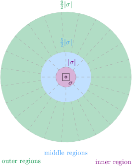
Figure 12: The regions defined by a cell $\sigma$.

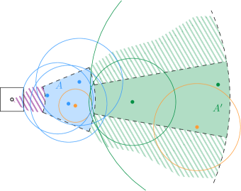
Figure 13: The set $S_{1}(A)$ is marked blue. The orange site in $A$ is not in the set because its radius it took small. The orange site in $A^{\prime}$ is not in $S_{1}(A^{\prime})$: while its radius is in the correct range, it does not touch or intersect the inner boundary.

We associate a set of sites $S_{1}(A)\subseteq S$ with each region $A\in\mathcal{A}_{\mathcal{T}}$, depending on the type of the region. This is done as follows: first, suppose that $A$ is an outer region for a cell $\sigma$. Then, the set $S_{1}(A)$ contains all sites $t$ such that

1. $t\in A$

2. $|\sigma|\leq r_{t}\leq 2|\sigma|$; and

3. $\|a(\sigma)t\|\leq r_{t}+\frac{5}{2}|\sigma|$.

This means that $t$ represents a disk whose size is comparable to $\sigma$, whose center lies in the region $A$, and that intersects the inner boundary of $A$. Second, if $A$ is a middle or the central region for a cell $\sigma$, then $S_{1}(A)$ contains all sites $t$ such that

1. $t\in A$; and

2. $|\sigma|\leq r_{t}<2|\sigma|$.

That is, the site $t$ represents a disk whose size is comparable to $\sigma$ and whose center lies in $A$. We define $\mathcal{A}\subseteq\mathcal{A}_{\mathcal{T}}$ to be the set of regions where $S_{1}(A)\neq\emptyset$. In the following, we will not strictly distinguish between a vertex from $\mathcal{A}$ and the corresponding region, provided that it is clear from the context.

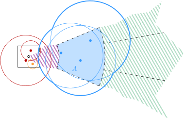
Figure 14: The red sites in $\sigma$ are in $S_{2}(A)$. The radius of the orange site is in the correct range, but it does not the intersect a site in $S_{1}(A)$ (marked blue).

Additionally for each region $A\in\mathcal{A}$ we define a set $S_{2}(A)$ as follows: Let $A$ be a region defined by a cell $\sigma$, then the set $S_{2}(A)$ contains all sites $s$ such that:

1. $s\in|\sigma|$

2. $s$ is adjacent in $\mathcal{D}(S)$ to at least one site in $S_{1}(A)$; and

3. $r_{s}<2|\sigma|$

We add an edge $\{s,A\}$ between a site and a region, if $s\in S_{1}(A)\cup S_{2}(A)$. Note that the sets $S_{1}(A)$ and $S_{2}(A)$ are not necessarily disjoint, as for the center region defined by a cell $\sigma$, a site with $|\sigma|\leq r_{s}<2|\sigma|$ will be both in $S_{1}(A)$ and $S_{2}(A)$. This will however influence neither the preprocessing time nor the correctness in a negative way.

The following structural lemma will help us both for showing that $H$ accurately represents the connectivity and also bounding the size of $H$ and the preprocessing time in the decremental setting.

Lemma 6.1.

Let $\{s,t\}$ be an edge in $\mathcal{D}(S)$ with $r_{s}\leq r_{t}$, then

1. there is a cell $\sigma\in N(t)$ such that $s\in\sigma$ and this cell defines a region $A$ with $t\in A$; and

2. all cells that define a region $A$ with $t\in S_{1}(A)$ are in $N(t)$.

Proof 6.2.

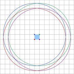
Figure 15: The disk $D(t,\frac{9}{2}|\sigma|)$ is contained in $N_{15\times 15}(\tau)$.

By assumption $\{s,t\}$ is an edge in $\mathcal{D}(S)$, and thus $\|st\|\leq r_{s}+r_{t}$. Let $\tau$ be the cell containing $t$ with $|\tau|\leq r_{t}<2|\tau|$. By the assumption on the radii, we have $r_{s}\leq r_{t}<2|\tau|$. Let $\sigma$ be the cell of the hierarchical grid with $|\sigma|=|\tau|$ and $s\in\sigma$. Using the triangle inequality this yields $\|a(\sigma)t\|\leq\frac{1}{2}|\sigma|+r_{s}+r_{t}<\frac{9}{2}|\sigma|$. Thus, the center of $\sigma$ has distance at most $\frac{9}{2}|\sigma|$ to $t$. Consider the disk $D=D\mathopen{}\mathclose{{}\left(t,\frac{9}{2}|\tau|}\right)$. All cells that can contain $s$ have their center in $D$. It suffice to show that $D$ is contained in $N(t)$, which is true, see Figure 15. By symmetry we also have $t\in D\mathopen{}\mathclose{{}\left(a(\sigma),\frac{9}{2}|\sigma|}\right)$. The regions defined by $\sigma$ partition this disk, and thus $t$ lies in one of the regions.

For the second claim, note that the only cells defining regions such that $t\in S_{1}(A)$ lie on the same level of the hierarchical grid as the cells in $N(t)$ by the condition on the radius. Furthermore, by the distance condition, the centers of the cells lie in the disk $D\mathopen{}\mathclose{{}\left(t,\frac{9}{2}|\sigma|}\right)$. The proof for the first property already showed that this disk is completely contained in $N(t)$.

Before we argue that our proxy graph $H$ accurately represents the connectivity of $\mathcal{D}(S)$, we first show that the associated sites of a region in $\mathcal{A}$ form a clique in $\mathcal{D}(S)$.

Lemma 6.3.

Suppose that $d_{1}\geq 23$ and $d_{2}\geq 8$. Then, for any region $A\in\mathcal{A}$, the associated sites in $S_{1}(A)$ form a clique in $\mathcal{D}(S)$.

Proof 6.4.

In the following, let $\sigma$ be the cell defining $A$. First, suppose that $A$ is an outer region. Let $t$ be a site in $S_{1}(A)$, and let $C$ be the cone that is centered at $a(\sigma)$ and was used to define $A$. Consider the line segments $\ell_{1}$ and $\ell_{2}$ that that go through $t$, lie in $C$, and are perpendicular to the upper and the lower boundary of $C$, respectively. We denote the endpoints of $\ell_{1}$ by $p_{1}$ and $p_{2}$, and the endpoints of $\ell_{2}$ by $q_{1}$ and $q_{2}$, where $p_{1}$ and $q_{1}$ are the endpoints at the right angles. See Figure 16 for an illustration.

We claim that both $\ell_{1}$ and $\ell_{2}$ are completely contained in $D_{t}$. Let $\alpha_{1},\alpha_{2}$ be the angles at $a(\sigma)$ defined by the line segment $\overline{a(\sigma)t}$ and the two boundaries of $C$. By our choice of $C$, we have $\alpha_{1}+\alpha_{2}=\frac{2\pi}{d_{1}}$.

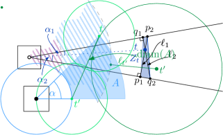
Figure 16: The line segment $\ell_{t^{\prime}}$ intersects $p_{2}q_{2}$.

Now we can compute the following lengths:

$$\|a(\sigma)q_{1}\| =\cos(\alpha_{1})\cdot\|a(\sigma)t\|$$

$$\|a(\sigma)p_{1}\| =\cos(\alpha_{2})\cdot\|a(\sigma)t\|$$

$$\|q_{1}q_{2}\| =\|a(\sigma)q_{1}\|\cdot\tan\mathopen{}\mathclose{{}\left(\frac{2\pi}{d_{1}}}\right)$$

$$\|p_{1}p_{2}\| =\|a(\sigma)p_{1}\|\cdot\tan\mathopen{}\mathclose{{}\left(\frac{2\pi}{d_{1}}}\right).$$

Combining these bounds, we get

$$\|\ell_{1}\| =\|p_{1}p_{2}\|=\tan\mathopen{}\mathclose{{}\left(\frac{2\pi}{d_{1}}}\right)\cdot\cos(\alpha_{2})\cdot\|a(\sigma)t\|$$

$$\|\ell_{2}\| =\|q_{1}q_{2}\|=\tan\mathopen{}\mathclose{{}\left(\frac{2\pi}{d_{1}}}\right)\cdot\cos(\alpha_{1})\cdot\|a(\sigma)t\|$$

The length of $\ell_{1}$ and $\ell_{2}$ are maximized for $\alpha_{2}=0$ or $\alpha_{1}=0$, respectively. This yields

$$\|\ell_{1}\|,\|\ell_{2}\| \leq\|a(\sigma)t\|\tan\mathopen{}\mathclose{{}\left(\frac{2\pi}{d_{1}}}\right)$$

$$\leq r_{t}+\frac{5}{2}|\sigma|\cdot\tan\mathopen{}\mathclose{{}\left(\frac{2\pi}{d_{1}}}\right)$$

$$\leq\frac{7}{2}r_{t}\cdot\tan\mathopen{}\mathclose{{}\left(\frac{2\pi}{d_{1}}}\right)$$

$$\leq r_{t}.$$

Thus, $\ell_{1}$ and $\ell_{2}$, as well as their convex hull $Z_{t}$, are completely contained in $D_{t}$.

Now, we take a closer look at the distance condition for the sites $t\in S_{1}(A)$. Recall that we require $\|a(\sigma)t\|\leq r_{t}+\frac{5}{2}|\sigma|$, or, equivalently, the disk $D_{t}$ must intersect or touch the disk $D\mathopen{}\mathclose{{}\left(a(\sigma),\frac{5}{2}|\sigma|}\right)$. As $\|a(\sigma)t\|\geq\frac{5}{2}|\sigma|$, the line segment $p_{2}q_{2}$ lies completely outside of $D\mathopen{}\mathclose{{}\left(a(\sigma),\frac{5}{2}|\sigma|}\right)$. Now consider the line segment $\ell_{t}=\overline{a(\sigma)t}\setminus D\mathopen{}\mathclose{{}\left(a(\sigma),\frac{5}{2}|\sigma|}\right)$. Equivalently, $\ell_{t}$ is the part of the line segment between $t$ and $a(\sigma)$ that lies outside of $D\mathopen{}\mathclose{{}\left(a(\sigma),\frac{5}{2}|\sigma|}\right)$. This line segment ends with a point on $D\mathopen{}\mathclose{{}\left(a(\sigma),\frac{5}{2}|\sigma|}\right)$. Now consider two sites $t$ and $t^{\prime}$ in $S_{1}(A)$. If $t^{\prime}$ lies in the convex hull $Z_{t}$, or if $t$ lies in the convex hull $Z_{t^{\prime}}$, we are done, as this directly implies that $t$ and $t^{\prime}$ are neighbors in $\mathcal{D}(S)$. Thus, assume without loss of generality that $t^{\prime}$ is separated from $a(\sigma)$ by the convex hull $Z_{t}$. Then, $\ell_{t^{\prime}}$ intersects $p_{2}q_{2}$, again inducing an edge $\{t,t^{\prime}\}$.

Next, suppose that $A$ is a middle region, and let $t,t^{\prime}\in S_{1}(A)$. By the definition of $S_{1}(A)$ we have $t,t^{\prime}\in A$. The law of cosines yields for $\operatorname{diam}(A)$

$$\operatorname{diam}(A)^{2} \leq|\sigma|^{2}+\mathopen{}\mathclose{{}\left(\frac{5}{2}|\sigma|}\right)^{2}-\frac{10}{2}|\sigma|^{2}\cos\mathopen{}\mathclose{{}\left(\frac{2\pi}{8}}\right)$$

$$\operatorname{diam}(A) \leq 2|\sigma|.$$

As we require that $r_{t},r_{t^{\prime}}\geq|\sigma|$, it follows that $\{t,t^{\prime}\}$ is an edge in $\mathcal{D}(S)$.

Finally, suppose that $A$ is an inner region and let $t,t^{\prime}\in A$. Since $t$ and $t^{\prime}$ both lie in the disk $D\mathopen{}\mathclose{{}\left(a(\sigma),|\sigma|}\right)$ of diameter $2|\sigma|$, and since $r_{t},r_{t^{\prime}}\geq|\sigma|$, we again get that the edge $\{t,t^{\prime}\}$ is present in $\mathcal{D}(S)$.

Having Lemmas 6.3 and 6.1 at hand, we can now show that $H$ accurately represents the connectivity of $\mathcal{D}(S)$.

Lemma 6.5.

Two sites $s,t\in S$ are connected in $H$ if and only if they are connected in $\mathcal{D}(S)$.

Proof 6.6.

First, we show that if $s$ and $t$ are connected in $H$, they are also connected in $\mathcal{D}(S)$. The path between $s$ and $t$ in $H$ alternates between vertices in $S$ and vertices in $\mathcal{A}$. Thus, it suffices to show that if two sites $u$ and $u^{\prime}$ are connected with the same region $A\in\mathcal{A}$, they are also connected in $\mathcal{D}(S)$. This follows directly from Lemma 6.3: if $u$ and $u^{\prime}$ both lie in $S_{1}(A)$, they are part of the same clique and thus adjacent. In the other case $S_{2}(A)$ is non-empty, there is at least one site in $S_{1}(A)$ which intersects the site in $S_{2}(A)$. Then $u$ is connected to $u^{\prime}$ via the clique induced by $S_{1}(A)$ and the claim follows.

Now, we consider two sites connected in $\mathcal{D}(S)$, and we show that they are also connected in $H$. It suffices to show that if $s$ and $t$ are adjacent in $\mathcal{D}(S)$, they are connected in $H$. Assume without loss of generality that $r_{s}\leq r_{t}$ and let $\sigma$ be the cell in $N(t)$ such that $s\in\sigma$.

This cell in $N(t)$ exists by the first property of Lemma 6.1 and was explicitly added to $\mathcal{T}$. We can thus conclude that $t\in S_{1}(A)$ for some $A\in\mathcal{A}_{\mathcal{T}}$. As the regions with non-empty sets $S_{1}(A)$ are in $\mathcal{A}$ by definition, the edge $\{t,A\}$ exists in $H$.

Now we argue that $s\in S_{2}(A)$ and thus the edge $\{A,s\}$ also exists in $H$. This follows by straightforward checking the properties of a site in $S_{2}(A)$. We have $s\in\sigma$ by the definition of $\sigma$ and by assumption the radius of $s$ is bounded by $r_{s}\leq r_{t}<2|\sigma|$. Finally, as $t$ is in $S_{1}(A)$ and $s$ and $t$ intersect, there is at least one site in $S_{1}(A)$ which intersects $s$ and we are done.

After we have shown that $H$ accurately represents the connectivity relation in $\mathcal{D}(S)$, we now show that the number of edge in $H$ depends only on $n$ and $\Psi$ and not on the number of edges in $\mathcal{D}(S)$ or the diameter of $S$. As the size of $H$ only depends on the number of sites in the sets $S_{1}(A)$ and $S_{2}(A)$, we first take a look at those sizes.

Lemma 6.7.

We have $\sum_{A\in\mathcal{A}}|S_{1}(A)|=O(n)$ and $\sum_{S\in\mathcal{A}}|S_{2}(A)|=O(n\log\Psi)$.

Proof 6.8.

For the first claim, we use the second property of Lemma 6.1, which tells us that $t$ can only lie in regions $A$ defined by cells in $N(t)$. There are $O(1)$ such cells and thus $t$ lies in at most $O(1)$ sets $S_{1}(A)$ and we get $\sum_{A\in\mathcal{A}}|S_{1}(A)|=O(n)$.

Next, we focus on the total size of all sets $S_{2}(A)$. A necessary condition for $s$ to lie in $S_{2}(A)$ is that $s$ lies in the cell defining $A$, so we focus on the cells containing $s$. There are potentially $O(\log(\operatorname{diam}(S)))$ cells in $\mathcal{T}$ that contain $s$. Recall however, that the set $\mathcal{A}$ only contains those cells, that have a non-empty set $S_{1}(A)$ and thus a diameter proportional to the sites in $S_{1}(A)$. As the maximum radius in $S$ is $\Psi$, the largest cell which is of interest has diameter $2^{\lfloor\log\Psi\rfloor}$ and all regions in $\mathcal{A}$ are defined by cells of the quadtree that lie below the level $\lfloor\log(\Psi)\rfloor+1$. For a fixed site this implies that it can lie in at most $O(\log\Psi)$ sets $S_{2}(A)$ and thus $\sum_{A\in\mathcal{A}}|S_{2}(A)|=O(n\log\Psi)$.

Corollary 6.9.

$H$ has $O(n)$ vertices and $O(n\log\Psi)$ edges.

Proof 6.10.

We can have at most $\sum_{A\in\mathcal{A}}|S_{1}(A)|$ non empty regions, and thus $|\mathcal{A}|=O(n)$. This constitutes the bound on the number of vertices. Furthermore, the number of edges is $\sum_{A\in\mathcal{A}}|S_{1}(A)|+|S_{2}(A)|=O(n\log\Psi)$.

6.2 Decremental Data Structure

Now we can describe how to use the graph $H$ defined in Section 6.1 to build a data structure that allows interleaved deletions and connectivity queries in a disk graph. The data structure will consist of several components: we store the quadforest containing $\mathcal{A}$ and we store the sets $S_{1}(A)$ and $S_{2}(A)$ for all regions $A\in\mathcal{A}$. For each region $A\in\mathcal{A}$ we store a reveal data structure (RDS) as defined in Corollary 5.12 with $S_{1}(A)$ as the set $B$ and $S_{2}(A)$ as the set $P$. Finally, we store the graph $H$ in a Holm et al. [19] data structure $\mathcal{H}$. See Figure 17 for an illustration of the data structure.

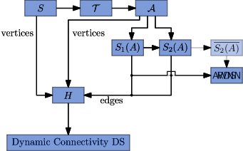
Figure 17: The structure of the decremental data structure

Our decremental data structure now works as follows. The queries are answered using $\mathcal{H}$. Now focus on the deletion of a site $s$. First, we delete all edges incident to $s$ from $\mathcal{H}$. Then, we consider all regions $A$ such that $s\in S_{1}(A)$. We remove $s$ from $S_{1}(A)$ and the RDS, and let $U$ be the set of revealed sites from $S_{2}(A)$ reported by the RDS. We delete each site $u\in U$ from $S_{2}(A)$ and the corresponding RDS. Additionally we delete the edges $\{u,A\}$ for $u\in U$ from $\mathcal{H}$ for all $u\in U$ that are not also in $S_{1}(A)$. Now, consider a region $A$ such that $s\in S_{2}(A)$. We simply remove $s$ from the set $S_{2}(A)$ and the associated RDS. First, we analyze the preprocessing time.

Lemma 6.11.

Given a site set $S$ we can preprocess the data structure described above in $O\mathopen{}\mathclose{{}\left(n\log^{5}n\lambda_{6}(\log n)+n\log\Psi\log^{3}n}\right)$ time.

Proof 6.12.

In a first step, we build the quadforest, containing the lowest $\lfloor\log\Psi\rfloor+1$ levels of the quadtree $\mathcal{T}$. For this we identify for each site in $S$ the cell of level $\lfloor{\log\Psi}\rfloor$ containing it. As we can identify the cell in $O(1)$ time, this takes $O(n)$ overall time. The lower $\lfloor\log\Psi\rfloor+1$ levels of $\mathcal{T}$ can now simple be constructed by building separate quadtrees for all non-empty cells created this way. As the height of each of these separate quadtrees is $O(\log\Psi)$, this takes an overall time of $O(n\log\Psi)$.

Now, there might be some cells in $\bigcup_{s\in S}N(s)$ that are not yet added to the forest. For each cell in $\bigcup_{s\in S}N(s)$, we can traverse the matching quadtree of the forest to find the position where the cell belongs to. If it is already in the quadtree we are done, in the other case we create a leaf and connect it to the quadtree with a matching path. This takes $O(\log\Psi)$ time for each cell, for an $O(n\log\Psi)$ overall time. In order to be able to identify the quadtree that contains a specific cell or site, we also build a binary search tree on the roots of the quadtrees, as described in Section 2. This takes an additional $O(n)$ time. Following the argument in the proof of Lemma 6.7 the cells in the quadforest are a superset of the cells in $\mathcal{A}$.

Now we are equipped to find the sets $S_{1}(A)$ and $S_{2}(A)$. Fix a site $t$. By Lemma 6.1 we only have to consider the regions defined by cells in $N(t)$ to find all sets $S_{1}(A)$ with $t\in S_{1}(A)$. For each cell in $N(t)$, we can iterate all regions defined by it, and find the sets $S_{1}(A)$ containing $t$ in constant time. Identifying the cells takes $O(\log n+\log\Psi)$ time for each cell in $N(t)$, for an overall $O(n(\log n+\log\Psi))$ time.

In order to be able to find the sets $S_{2}(A)$, we build a static additively weighted data nearest neighbor data structure on all sets $S_{1}(A)$. Each site $t\in S_{1}(A)$ has weight $-r_{t}$. By Lemma 2.7, these data structures can be constructed in $O\mathopen{}\mathclose{{}\left(|S_{1}(A)|\log n}\right)$ time each, while allowing a query time of $O(\log n)$. As $\sum_{A\in\mathcal{A}}=O(n)$ by Lemma 6.7, we need $O(\sum_{A\in\mathcal{A}}|S_{1}(A)|\log n)=O(n\log n)$ time to compute all data structures. For a site $s\in S$, let $\pi_{s}$ be the path in $\mathcal{T}$ from the root to the cell $\sigma_{s}$ with $s\in\sigma_{s}$ and $|\sigma_{s}|\leq r_{s}<2|\sigma_{s}|$. For each cell along $\pi_{s}$, we query all nearest neighbor data structures with $s$. If $s$ intersects the reported weighted nearest neighbor, we add it to $S_{2}(A)$. As we use the negative additive weight for the nearest neighbor data structure, we do not miss a site this way [25, Lemma 2.8]. Each site $s$ is used for $O(\log\Psi)$ queries, for an overall of $O(n\log n\log\Psi)$ time to find all sets $S_{2}(A)$.

The edges of $H$ are now determined by the sets $S_{1}(A)$ and $S_{2}(A)$. We insert the edges one by one to an initially empty Holm et al. data structure and obtain the connectivity data structure $\mathcal{H}$ in overall $O\mathopen{}\mathclose{{}\left(n\log\Psi\log^{2}n}\right)$ time.

Having the sets $S_{1}(A)$ and $S_{2}(A)$ at hand, by Corollary 5.12 we can build the RDS with $B=S_{1}(A)$ and $P=S_{2}(A)$ in $O\mathopen{}\mathclose{{}\left(|S_{1}(A)|\log^{5}(n)\lambda_{6}(\log(n))+|S_{2}(A)|\log^{3}(n)}\right)$ expected time for each region $A\in\mathcal{A}$. The total time is then dominated by summing over all regions and using Lemma 6.7:

$$\leavevmode\nobreak\ \leavevmode\nobreak\ \phantom{=}O\mathopen{}\mathclose{{}\left(\sum_{A\in\mathcal{A}}|S_{1}(A)|\log^{5}(n)\lambda_{6}(\log n)+|S_{2}(A)|\log^{3}(n)}\right)$$

$$=O\mathopen{}\mathclose{{}\left(\mathopen{}\mathclose{{}\left(\sum_{A\in\mathcal{A}}|S_{1}(A)|}\right)\cdot\log^{5}(n)\lambda_{6}(\log n)+\mathopen{}\mathclose{{}\left(\sum_{A\in\mathcal{A}}|S_{2}(A)|}\right)\cdot\log^{3}(n)}\right)$$

$$=O\mathopen{}\mathclose{{}\left(n\log^{5}n\lambda_{6}(\log n)+n\log\Psi\log^{3}(n)}\right)$$

Now we show that the data structure is correct and efficiently handles the queries.

Theorem 6.13.

The data structure described above handles $m$ site deletions in overall $O\mathopen{}\mathclose{{}\left(\mathopen{}\mathclose{{}\left(n\log^{5}n}\right.}\right.+\mathopen{}\mathclose{{}\left.\mathopen{}\mathclose{{}\left.m\log^{9}n}\right)\lambda_{6}(\log n)}\right.+\mathopen{}\mathclose{{}\left.n\log\Psi\log^{4}n}\right)$ time. Furthermore, it correctly answers connectivity queries in $O(\frac{\log n}{\log\log n})$ amortized time.

Proof 6.14.

We first show that the answers given by our data structure are indeed correct. During the lifetime of the data structure we maintain the invariant, that the sets $S_{1}(A)$ and $S_{2}(A)$ always contain the sites as defined in Section 6.1, the graph stored in $\mathcal{H}$ is the proxy graph $H$ and each RDS associated with a region $A$ contains the sets $S_{1}(A)$ and $S_{2}(A)$. Assuming that this invariant holds, Lemma 6.5 implies that the answers given for each query are correct.

To show that the invariant is maintained, we first note that removing a site from a set $S_{2}(A)$, does only lead to the deletion of a single edge from $H$. As we make sure to mirror the removal from $S_{2}(A)$ in $\mathcal{H}$ and the RDS, removing a newly deleted site $s$ from all sets $S_{2}(A)$ containing it, maintains the invariant. Now let $A$ be a region, such that the newly deleted site $s$ lies in $S_{1}(A)$. Then for all sites in the matching set $S_{2}(A)$, it is necessary to intersect at least one site in $S_{1}(A)$. Furthermore, there is an, possibly empty, subset $U^{\prime}$ of sites in $S_{2}(A)$ that only intersect $s$. So to maintain the invariant, we have to delete these sites from $S_{2}(A)$ and the matching RDS. As these sites are exactly the sites reported in the set $U$ returned by the RDS, $U^{\prime}$ is removed by definition, and the invariant on $S_{2}(A)$ and the RDS is maintained. As we do not delete the edges that were present because a site was in $S_{1}(A)\cap S_{2}(A)$, the graph stored in $\mathcal{H}$ is still the proxy graph $H$ and the invariant is maintained.

Now, we can focus on the analysis of the running time. Queries are performed in $\mathcal{H}$ with a amortized running time of $O(\frac{\log n}{\log\log n})$. Each edge is removed exactly once from $\mathcal{H}$, for a total of $O\mathopen{}\mathclose{{}\left(n\log\Psi\log^{2}n}\right)$ time. Finding the regions $A$ whose sets $S_{1}(A)$ and $S_{2}(A)$ have to be updated takes again $O(\log n+\log\Psi)$ time in each deletion, by similar argument as in the proof of Lemma 6.11. The steps dominating the running time are the deletions from the RDS. By Corollary 5.12, the RDS associated to a single region, adds at most a running time of $O\mathopen{}\mathclose{{}\left(\mathopen{}\mathclose{{}\left(|S_{1}(A)|\log^{5}n+m_{A}\log^{11}n}\right)\lambda_{6}(\log n)+|S_{2}(A)|\log^{4}n}\right)$ to the total running time, where $m_{A}$ is the number of sites deleted from $S_{1}(A)$. Summing over all regions, we have $\sum_{A\in\mathcal{A}}m_{A}=O(m)$ as each site is contained in $O(1)$ sets $S_{1}(A)$. Furthermore, as we have $\sum_{A\in\mathcal{A}}|S_{1}(A)|=O(n)$ and $\sum_{A\in\mathcal{A}}|S_{2}(A)|=O(n\log\Psi)$, the total running time of $O\mathopen{}\mathclose{{}\left(\mathopen{}\mathclose{{}\left(n\log^{5}n+m\log^{9}n}\right)\lambda_{6}(\log n)+n\log\Psi\log^{4}n}\right)$ for $m$ deletions follows.

6.3 Incremental Data Structure

In this section, we introduce the incremental dynamic connectivity data structure for the bounded radius ratio case. Again, the data structure is based on our proxy graph $H$ as described in Section 6.1. As we only do insertions, we use the connectivity data structure from Theorem 2.1 for $\mathcal{H}$. This data structures, achieves amortized time $O\mathopen{}\mathclose{{}\left(1}\right)$ for updates and $O\mathopen{}\mathclose{{}\left(\alpha(n)}\right)$ for queries [24].

To be able to update the edges incident to a region $A$, defined by a cell, we use two fully dynamic additively nearest neighbor data structures (Lemma 2.7) one on the set $S_{1}(A)$, and one on the site set $\overline{S_{2}(A)}$ that contains those sites in $\sigma$ with radius $r<2|\sigma|$ that have not been added to $S_{2}(A)$ yet. Finally, we maintain an underlying quadforest of height $\lfloor\log\Psi\rfloor+1$ to track the present cells. See Figure 18 for an illustration of the data structure.

Figure 18: The structure of the decremental data structure

Now, the data structure works as follows: when inserting a site $s$, we determine the cells of the neighborhood $N(s)$. Then, we add all cells to the quadforest that are not contained yet. Furthermore, we add the associated region vertices to $H$ and also to the dynamic connectivity graph structure $\mathcal{H}$. Afterwards, we have to connect the site $s$ to the regions. Hence, we have to identify the sets $S_{1}(A)$, $S_{2}(A)$, and $\overline{S_{2}(A)}$ the site $s$ belongs to, add $s$ to the corresponding AWNN, and insert the edges incident to $s$ to $\mathcal{H}$. After the insertion of $s$ in $S_{1}(A)$, we also query the AWNN of the associated $\overline{S_{2}(A)}$ to find the sites that intersect $s$ and thus have to be transferred to $S_{2}(A)$, do so if required and add the edges incident to the transferred site to $\mathcal{H}$.

Theorem 6.15.

The data structure described above correctly answers connectivity queries in $O(\alpha(n))$ amortized time and insertions in $O(\log\Psi\lambda_{6}(\log n)\log^{9}n)$ amortized expected time, where $n$ is the number of sites stored in the data structure.

Proof 6.16.

First, we show that the described data structure answers connectivity queries correctly. We use similar invariants as in the proof of Theorem 6.13:

1. The AWNN of $S_{1}(A)$ contains exactly the sites in $S_{1}(A)$,

2. the AWNN $\overline{S_{2}(A)}$ contains exactly the sites that would lie in $S_{2}(A)$ if there was a disk in $A$ intersecting them,

3. the sets $S_{1}(A)$ and $S_{2}(A)$ in our data structure always contain the sites as defined in Section 6.1; and

4. the graph stored in $\mathcal{H}$ is the proxy graph $H$.

Note that we implicitly store the set $S_{2}(A)$ in the data structure $\mathcal{H}$. Since no sites are deleted from $S_{2}(A)$ and we never query against sites in $S_{2}(A)$ we do not have to store $S_{2}(A)$ in an auxiliary data structure. Under the assumption that the invariants hold, Lemma 6.5 again implies that the answers given for each query are correct.

Invariant 1 and the first part of Invariant 3 hold by definition. When inserting a site $s$ it is added to all sets $S_{1}(A)$ of regions $A$, with $s\in A$ in $N(s)$ it belongs to. By Lemma 6.1 these are the only regions potentially containing $s$. When locating $s$ in $S_{1}(A)$, $s$ is added to the AWNN of $S_{1}(A)$ and the edge $(s,A)$ is inserted into $\mathcal{H}$. This exactly represents the edge we would have in $H$. To complete the proof of invariants 3 and 4, we first need to prove that Invariant 2 holds.

By definition of $S_{2}(A)$, we can only insert sites with $s\in|\sigma|$, radius $r_{s}<2|\sigma|$ and the constraint that $s$ is adjacent in $\mathcal{D}(S)$ to at least one site in $S_{1}(A)$. Furthermore, we add a site to $\overline{S_{2}(A)}$, when it fulfills the first two but not the last constraint. This guarantees that a site $s$ is potentially present in the sets $S_{2}(A)$ of the regions defined by any cell on the path from the root to $\sigma_{s}$, as these are exactly the cells for which the radius constraint of $S_{2}(A)$ holds. We check for all those regions, if $s$ intersects any site in $S_{1}(A)$. The site is only inserted into $S_{2}(A)$ if there is an intersection otherwise it is added to the AWNN of $\overline{S_{2}(A)}$. Furthermore, a site in $\overline{S_{2}(A)}$ is only transferred from $\overline{S_{2}(A)}$ to $S_{2}(A)$ if a newly inserted site in $S_{1}(A)$ intersects it which proves Invariant 2. Whenever we assign a site to a region $S_{2}(A)$, during its insertion or because of a change of the corresponding set $S_{1}(A)$, we add the edge $(s,A)$ to $\mathcal{H}$ representing the edge we need to have in $H$. This also concludes the proof of Invariants 3 and 4 and thus the correctness.

Now, we consider the running time of the data structure. When inserting a site $s$, we first have to identify the grid cell in level $\lfloor\log\Psi\rfloor+1$ it belongs to, that is the cell representing the root of the quadtree containing $\sigma_{s}$. After the root cell is found, we look up the cell $\sigma_{s}$ in the quadtree. As defined in Section 2, this takes $O\mathopen{}\mathclose{{}\left(\log n+\log\Psi}\right)$ time, where $n$ is the number of sites contained in $\mathcal{H}$ at the time of the insertion.

We distinguish two cases: either $\sigma_{s}$ already exists in the quadforest, or we have to insert it. In the latter case, we extend the quadtree during the search step as follows: when we reach a leaf in the quadtree during the search and did not arrive at the level of $\sigma_{s}$, we add its four children to the former leaf. We then step down into the newly created leaf that contains $\sigma_{s}$ and repeat the process until we added $\sigma_{s}$.

Note that it is possible that even the root of the quadtree containing $\sigma_{s}$ does not exist. In this case, we insert the root cell into the balanced binary search tree and create a root node before processing the way down as described before. As the insertion into the search tree takes $O\mathopen{}\mathclose{{}\left(\log n}\right)$ time just as in the look-up step, this does not increase the running time. Additionally, the operation of searching for $\sigma_{s}$ or accordingly building the quadtree downwards to the level of $\sigma_{s}$ requires at most $O\mathopen{}\mathclose{{}\left(\lfloor\log\Psi\rfloor}\right)$ time which is the maximum height of the quadtrees in the forest.

To complete the insertion of $s$ in the forest component, we also have to introduce the cells of the neighborhood $N_{15\times 15}(\sigma_{s})$ if not present yet. Here, the look-up operation as well as the insertion, if required, are executed in a similar manner as for $\sigma_{s}$. Since the neighborhood is of constant size, the overall processing time of the quadtree forest during the insertion of $s$ is in $O\mathopen{}\mathclose{{}\left(\log n+\log\Psi}\right)$.

When introducing cells into the forest, we also need their associated regions to be present in the proxy graph $H$. Hence, we insert the regions of the new cells as isolated vertices to $\mathcal{H}$ and initialize the corresponding AWNN of the regions for $S_{1}(A)$ and $\overline{S_{2}(A)}$. Subsequently, we have to insert $s$ itself and its edges as follows: first, we add $s$ as an isolated vertex to $\mathcal{H}$. Then, we insert $s$ to the sets containing it and if applicable the associated AWNN. Since we implicitly store $S_{1}(A)$ and $S_{2}(A)$, we add the corresponding edges between the regions and $s$ to $\mathcal{H}$ along the way.

Recall, that by Lemma 6.1, $s$ can only be in a set $S_{1}(A)$ defined by a cell in $N(s)$. Therefore, we iterate through the cells of $N(s)$ and add $s$ with weight $-r_{s}$ to the AWNN of the sets $S_{1}(A)$ it belongs to. We also introduce the respective edges $(s,A)$ to the proxy graph. As $N(s)$ is of constant size this step takes $O(1)$ amortized time for the insertion of edges in $\mathcal{H}$ and $O(\lambda_{6}(\log n)\log^{5}n)$ expected time for insertions into the AWNN.

Furthermore, for a region $A$ changes in a set $S_{1}(A)$ may affect the set $S_{2}(A)$. Hence, we have to check if the insertion of $s$ into $S_{1}(A)$ yields a transfer of a site $t$ from $\overline{S_{2}(A)}$ to $S_{2}(A)$ because $D_{s}$ intersects $D_{t}$. We identify these sites by iteratively doing a weighted nearest neighbor search with $s$ on the AWNN on $\overline{S_{2}(A)}$ until we do not find a site intersecting $s$ anymore. When finding a site $t$ intersecting $s$, we delete $t$ from the AWNN on $\overline{S_{2}(A)}$ and introduce the edge $(t,A)$ into $\mathcal{H}$. The amortized expected running time of $O(\lambda_{6}(\log n)\log^{9}n)$ to delete a site from $\overline{S_{2}(A)}$ dominates this step. We do not know how many deletions are required in this step, but a site $t$ can be present in the most $O(\log\Psi)$ sets $\overline{S_{2}(A)}$, associated to the cells containing $t$ on the path from the root to $\sigma_{t}$. Furthermore, a site $t$ is only inserted into $\overline{S_{2}(A)}$, when $t$ is inserted. Thus, these deletions take overall $O(n\log\Psi\lambda_{6}(\log n)\log^{9}n)$ expected time, which yields an amortized expected running time of $O(\log\Psi\lambda_{6}(\log n)\log^{9}n)$ per insertion.

Now, we consider the time needed to insert of $s$ either into $S_{2}(A)$ or $\overline{S_{2}(A)}$. By definition, we know that $s$ has to be added either to $S_{2}(A)$ or to $\overline{S_{2}(A)}$ of the regions of the cells along the path from the root to $\sigma_{s}$ in the quadtree. Let $A$ be a region defined by a cell along this path. To determine whether to add $s$ to $S_{2}(A)$ or to $\overline{S_{2}(A)}$, we perform a nearest neighbor search on the AWNN of $S_{1}(A)$. If we find a site in $S_{1}(A)$ intersecting $s$, we know that $s$ belongs to $S_{2}(A)$. Then, we insert the edge $(s,A)$ to $\mathcal{H}$, if it does not exist yet. This takes $O(1)$ amortized time. In the other case, $s$ is inserted to the AWNN of $\overline{S_{2}(A)}$ in $O(\lambda_{6}(\log n)\log^{5}n)$ amortized expected time. This last step concludes the insertion. Since each cell defines a constant number of regions, the step requires a constant number of look-up and insertion operations on each level. As the time for insertions into the AWNN of $\overline{S_{2}(A)}$ dominates, the last insertion step yields an amortized expected running time of $O(\log\Psi\lambda_{6}(\log n)\log^{5}n)$

By the summing over all insertion steps, we achieve an amortized expected running time of $O(\log\Psi\lambda_{6}(\log n)\log^{9}n)$ per insertion because of the dominating running time of the deletions from $\overline{S_{2}(A)}$.

It remains to consider the running time for the query which directly follows from the query time in $\mathcal{H}$. This concludes our proof.

7 Arbitrary Radius Ratio

In this section, we extend the approach from Section 6 to give a data structure that allows update times independent of $\Psi$. The cost for dropping the dependence on $\Psi$ is exchanging the additive $O\mathopen{}\mathclose{{}\left(n\log\Psi\log^{4}n}\right)$ term in the running time in Theorem 6.13 with an additional $O(\log n)$ factor in the first term. The additive $O\mathopen{}\mathclose{{}\left(n\log\Psi\log^{4}n}\right)$ part in Section 6 came from the size of the sets $S_{2}(A)$ and thus from the height of each quadtree in the forest of quadtrees. We can get rid of this dependency by using a compressed quadtree $\mathcal{Q}$. Recall from Section 2 that the height and size of the compressed quadtree do not depend on the diameter of the point set, but only on $n$. However the height of $\mathcal{Q}$ can still be $O(n)$ which is not favorable for our application. In order to reduce the number of edge in our proxy graph to $O\mathopen{}\mathclose{{}\left(\log^{2}n}\right)$, we consider a heavy path decomposition on $\mathcal{Q}$ in combination with binary search trees for each heavy path. The new proxy graph is described in Section 7.1 and the decremental connectivity data structure based on this graph can be found in Section 7.2.

7.1 The Proxy Graph

The main structure of the proxy graph is the same as that described in Section 6.1, so we will often refer back to it. We still have a bipartite graph with the sites from $S$ on one side and a set of region on the other side. The regions will again be used to define sets $S_{1}(A)$ and $S_{2}(A)$ that will in turn define the edges. However we adapt the definition of the regions and define them based on certain paths of the compressed quadtree instead of single cells. Furthermore, we relax the condition on the radii in the definition of the set $S_{1}(A)$.

Similar to the non-compressed approach, we consider an augmented version of the quadtree. Again let $N(s)$ be the $15\times 15$ neighborhood of the cell $\sigma$ containing $s$ such that $|\sigma|\leq r_{s}<2|\sigma|$. Instead of working with the compressed quadtree on the sites, we work on the tree $\mathcal{Q}$ that also contains all cells which are part of at least one neighborhood.

Now let $\mathcal{R}$ be the heavy path decomposition of $\mathcal{Q}$. For each heavy path $R\in\mathcal{R}$, we find a set $\mathcal{P}_{R}$ of canonical paths such that every subpath of $P$ can be written as the disjoint union of $O(\log n)$ canonical paths. To be precise, for each $R\in\mathcal{R}$ we build a balanced binary search tree with the cells of the path in the leafs, sorted by increasing diameter. We associate each vertex $v$ in the binary search tree with the path induced by all cells in the subtree rooted at $v$ and add this path to $\mathcal{P}_{R}$. Using this definition, we can now write every path in $\mathcal{Q}$ that starts at the root as the disjoint union of canonical path, as shown in the following lemma:

Lemma 7.1.

Let $\sigma$ be a vertex of $\mathcal{Q}$ and let $\pi$ be the path from the root of $\mathcal{Q}$ to $\sigma$. Then there exists a set $\mathcal{P}_{\pi}$ of canonical paths such that:

1. $|\mathcal{P}_{\pi}|=O\mathopen{}\mathclose{{}\left(\log^{2}n}\right)$; and

2. $\pi$ is the disjoint union of the canonical paths in $\mathcal{P}_{\pi}$.

Proof 7.2.

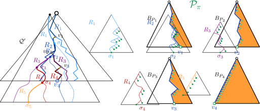
Figure 19: Illustration of Lemma 7.1. Left we see the decomposition of $R$ into $R_{1},\dots R_{k}$. On the right the vertices defining $\mathcal{P}_{\pi}$ are depicted in green.

Consider the heavy paths $R_{1},\dots,R_{k}$ encountered along $\pi$. By Lemma 2.4 we have that $k\in O(\log n)$ and that $\pi$ is the disjoint union of the intersections $\pi\cap R_{i}$. Each of these intersections constitutes a subpath of $R_{i}$ whose largest cell is also the largest cell of $R_{i}$. Let $\sigma_{i}$ be the smallest cell of $\pi\cap R_{i}$, then the subpath of $R_{i}$ consists of all cells in $R_{i}$ having diameter at least $|\sigma_{i}|$. This subpath can be composed as the disjoint union of all canonical paths defined by the right children along the search path for $\sigma_{i}$ in the binary search tree associated with $R_{i}$, together with the path only consisting of $\sigma_{i}$; see Figure 19. As the height of a balanced binary search tree is $O(\log n)$, the overall number of canonical paths needed to represent $\pi$ is $O(\log^{2}n)$.

The vertex set of the proxy graph $H$ again consists of the set of sites $S$ and a set of regions $\mathcal{A}$. We define $O(1)$ regions for each canonical path in a similar way as we defined the regions in Section 6.1. Let $\sigma$ be the smallest cell and $\tau$ be the largest cell of a canonical path. The inner and middle regions are defined as in the bounded case, using the smallest cell of the path to define the region, instead of the single cell in Section 6.1. That is the inner region is the disk with center $a(\sigma)$ and radius $|\sigma|$. The middle regions are the $d_{2}$ regions which are defined as the intersection of the cones in $\mathcal{C}_{d_{2}}$ with the annulus with inner radius $|\sigma|$ and outer radius $\frac{5}{2}{|\sigma|}$. For the outer regions, we extend the outer radius of the annulus. They are defined as the intersections of the cones in $\mathcal{C}_{d_{1}}$ with the annulus of inner radius $\frac{5}{2}{|\sigma|}$ and outer radius $\frac{5}{2}|\sigma|+2|\tau|$, again centered at $a(\sigma)$. The set $\mathcal{A}$ now contains the regions defined this way for all canonical paths.

Given a region $A\in\mathcal{A}$ with smallest cell $\sigma$ and largest cell $\tau$, we can now define the sets $S_{1}(A)$ and $S_{2}(A)$. The set $S_{1}(A)$ is defined similarly to the set in Section 6.1, again using $\sigma$ in the role of the single cell for most parts. The difference is that the radius range for $t$ is larger, as it’s upper bound depends on the largest cell of the path. The set $S_{1}(A)$ contains all sites $t$ such that

1. $t\in A$

2. $|\sigma|\leq r_{t}\leq 2|\tau|$; and

3. $\|a(\sigma)t\|\leq r_{t}+\frac{5}{2}|\sigma|$.

The last condition is only relevant, if $A$ is an outer region, as it is trivially true for middle and inner regions.

The definition for $S_{2}(A)$ is also similar to that in Section 6.1, however the difference in its definition are larger than for the set $S_{1}(A)$. Let $\sigma_{s}$ be the the cell such that $s\in\sigma_{s}$ and $|\sigma_{s}|\leq r_{s}<2|\sigma_{s}|$, let $\pi_{s}$ be the path in $\mathcal{Q}$ from the root to $\sigma_{s}$ and let $\mathcal{P}_{\pi_{s}}$ be the decomposition of $\pi_{s}$ into canonical paths as defined in Lemma 7.1. Let $A$ be a region, defined by a canonical path $P$, then $s\in S_{2}(A)$ if

1. $P\in\mathcal{P}_{\pi_{s}}$; and

2. $s$ is adjacent in $\mathcal{D}(S)$ to at least one site in $S_{1}(A)$.

If $\sigma$ is the smallest cell in a canonical path defining a region $A$, then each site $s$ in $S_{2}(A)$ lies in $\sigma$, has a radius less than $2|\sigma|$ and intersects at least one cell in $S_{2}(A)$. These are basically the conditions we had in Section 6.1. However, as the definition is restricted to those canonical paths in $\mathcal{P}_{\pi_{s}}$, not all sites satisfying these conditions are considered. As we will see below, this suffices to make sure that the proxy graph represents the connectivity, while also ensuring that each site $s$ lies in few sets $S_{2}(A)$.

The graph $H$ is now again defined by connecting a site $s\in S_{1}(A)\cup S_{2}(A)$ to the region $A$. To show that $H$ accurately represents the connectivity in $D(S)$, we need the following corollary from Lemma 6.3.

Corollary 7.3.

Suppose that $d_{1}\geq 23$ and $d_{2}\geq 8$. Then, for any region $A\in\mathcal{A}$, the associated sites in $S_{1}(A)$ form a clique in $\mathcal{D}(S)$.

Proof 7.4.

Recall that the center of the annuli and disks defining $A$ is the smallest cell of the associated canonical path. A close inspection of the proof for Lemma 6.3 shows that we only use the lower bound on the radii of the sites in $S_{1}(A)$. As this lower bound is unchanged, all arguments carry over for sites with larger radii.

Lemma 7.5.

Two sites $s$ and $t$ are connected in $\mathcal{D}(S)$ if and only if they are connected in $H$.

Proof 7.6.

If $s$ and $t$ are connected in $H$, the same argument as in the proof of Lemma 6.5 with Corollary 7.3 instead of Lemma 6.3 holds. The more challenging part is to show that if two sites are connected in $\mathcal{D}(S)$ they are also connected in $H$.

Figure 20: The cell $\sigma_{s}$ is the smallest cell such that $r_{s}\leq 2|\sigma_{s}|$. The canonical path $P$ contains $\rho$.

If suffices to show that if $s$ and $t$ are connected by an edge in $\mathcal{D}(S)$, they are connected to the same region $A\in\mathcal{A}$. Refer to Figure 20 for a depiction of the following argument. Assume without loss of generality that $r_{s}\leq r_{t}$. Consider the neighborhood $N(t)$ of $t$. Then by Lemma 6.1 there is a cell $\rho\in N(t)$ that contains $s$. Consider the path $\pi_{s}$ in $\mathcal{Q}$ from the root to the cell $\sigma_{s}$ such that $s\in\sigma_{s}$ and $|\sigma_{s}|\leq r_{s}<2|\sigma_{s}|$. The cell $\sigma_{s}$ is in $\mathcal{Q}$ as it is part of $N(s)$. Then $\rho$ lies on this path $\pi_{s}$. Let $\mathcal{P}_{\pi_{s}}$ be the decomposition of $\pi_{s}$ into canonical paths as defined in 7.1 and let $P$ be the path containing $\rho$. Let $\sigma$ and $\tau$ be the smallest and largest cell on $P$ respectively. By the definition of $P$, we have $\sigma_{s}\subseteq\sigma\subseteq\rho\subseteq\tau$. As $\{s,t\}$ is an edge in $D(S)$, we have $\|st\|\leq r_{s}+r_{t}\leq 2|\sigma|+2|\tau|$ and thus $\|a(\sigma)t\|\leq\frac{5}{2}|\sigma|+2|\tau|$. This implies that $t$ lies in a region $A$ defined by $P$ and thus $t\in S_{1}(A)$ for this region. As $s$ intersects $t$, it intersects at least one site in $S_{1}(A)$ for the region $A$. Furthermore, $P$ is a canonical path in $\mathcal{P}_{\pi_{s}}$ and thus $s\in S_{2}(A)$ by definition. As $s,t\in S_{1}(A)\cup S_{2}(A)$, they are connected in $H$.

Lemma 7.7.

The graph $H$ has $O(n)$ vertices and $O\mathopen{}\mathclose{{}\left(n\log^{2}n}\right)$ edges.

Proof 7.8.

As discussed in Section 2 the compressed quadtree consists of $O(n)$ cells. Each cell is part of exactly one heavy path, so the total size of the binary search trees that define the canonical paths is $O(n)$. A balanced binary search tree with $n$ leafs has $O(n)$ inner vertices, and thus there is a total of $O(n)$ canonical paths. As each canonical path defines $O(1)$ regions, the number of regions and therefore also the number of vertices in $H$ follows.

To bound the number of edges, we again count the number of sets $S_{1}(A)$ and $S_{2}(A)$ a single sites can be contained in. Again let $\sigma$ and $\tau$ be the smallest and largest cell of a canonical path respectively. A site $t$ can only be in a set $S_{1}(A)$ if $|\sigma|\leq r_{t}\leq 2|\tau|$ and $\sigma$ is contained in a cell of $N(t)$. To see the second claim, let $P$ be a canonical path such that $t\in S_{1}(A)$ for a region $A$ defined by $P$ and let $\sigma$ be the smallest cell of $P$. If $|\sigma|\leq r_{t}<2|\sigma|$, the statement holds by the second property given in Lemma 6.1. In the other case, let $\rho$ be the cell of the hierarchical grid with $|\sigma|<|\rho|\leq r_{t}<2|\rho|$ and $\sigma\subseteq\rho$. As $t\in S_{1}(A)$, we have

$$\|ta(\sigma)\| \leq r_{t}+\frac{5}{2}|\sigma|$$

$$\leq 2|\rho|+\frac{5}{4}|\sigma| \text{since }r_{t}\leq 2|\rho|\text{ and }|\sigma|\leq 2|\rho|$$

$$\leq\frac{13}{4}|\rho|$$

$$\|ta(\rho)\| \leq\frac{15}{4} \text{by triangle inequality as }\sigma\subseteq\rho$$

By the same considerations as in the proof of Lemma 6.1, it follows that $\rho\in N(t)$ and thus $\rho$ is in $\mathcal{Q}$ and also in $P$.

Let $\rho$ be a cell of $N(t)$, and let $R$ be the heavy path containing $\rho$. Then $t$ is considered for the set $S_{1}(A)$ for all regions which are defined by a canonical path containing $\rho$. These are the $O(\log n)$ paths along the search path for $\rho$ in the binary search tree on the cells of $R$ and thus each site can be part of at most $O(\log n)$ sets $S_{1}(A)$.

The number of sets $S_{2}(A)$, a fixed site $s$ can be part of, is at most the number of canonical paths decomposing the path from the root to the smallest cell containing $s$. By Lemma 7.1 there are $O\mathopen{}\mathclose{{}\left(\log^{2}n}\right)$ such paths. This yields $\sum_{A\in\mathcal{A}}|S_{1}(A)|+|S_{2}(A)|=O\mathopen{}\mathclose{{}\left(n\log^{2}n}\right)$ as an upper bound for the number of edges.

7.2 Decremental Data Structure

The structure of the decremental data structure is the same as in Section 6.2, recall Figure 17. We again store the sets $S_{1}(A)$ and $S_{2}(A)$ together with a RDS for each region $A$. The set $B$ for the RDS is again $S_{1}(A)$ and the set $P$ is $S_{2}(A)$. Furthermore, we store the graph $H$ defined by $S_{1}(A)$ and $S_{2}(A)$ in a Holm et al. data structure $\mathcal{H}$.

Both queries and deletions work exactly as in Section 6.2, however we repeat them here for completeness. Queries are performed on $\mathcal{H}$. On the deletion of a site $s$, we first remove all edges incident to $s$ from $\mathcal{H}$. Then the site is removed from all sets $S_{1}(A)$ containing it, as well as the associated RDS. The sites $U$ reported as revealed by the RDS are then removed from the matching $S_{2}(A)$ and the edges $\{u,A\}$ for $u\in U\setminus S_{1}(A)$ are removed from $\mathcal{H}$. Finally the site $s$ is removed from all sets $S_{2}(A)$ and the matching RDS.

Lemma 7.9.

The data structure described above can be preprocessed in $O(n\log^{6}n\lambda_{6}(\log n))$ time.

Proof 7.10.

To find the regions $\mathcal{A}$ we first compute the extended compressed quadtree $\mathcal{Q}$. This can be done by adding $O(n)$ virtual sites to our site set, similar to a construction of Har-Peled [16]. For each site $s\in S$ and each cell $\sigma\in N(s)$ we add two virtual sites. The virtual sites are added at the center of two of the cells one level below $\sigma$ that are contained in $\sigma$, see Figure 21 for an illustration. Now, all cells in $N(s)$ have at least two children in the non-compressed quadtree and thus the cells are also present in the compressed quadtree. When having $\mathcal{Q}$ at hand, we can, with additional $O(n)$, time find the heavy paths by Item 3. of Lemma 2.4, and the binary search trees on the heavy paths by standard techniques. This gives us the set of regions $\mathcal{A}$.

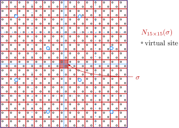
Figure 21: Four cells from $N_{15\times 15}(\sigma)$ with the virtual sites

To find the set $S_{1}(A)$, recall that a site $t$ can only lie in the set $S_{1}(A)$ for a region defined by a canonical path that contains a cell in $N(t)$. The sets $S_{1}(S)$ we can now be found as follows. For each site $t\in S$, compute the cells in $N(t)$ and for each such cell $\rho$ find the heavy path $R$ containing it. In the binary search tree defined on $R$, follow the search path for $\rho$ and for each canonical path defined along this search path explicitly find the region containing $t$ and check if the distance condition holds.

When implementing this step naively it takes $O\mathopen{}\mathclose{{}\left(n\log^{2}n}\right)$ time which is fast enough for our purposes. We could however reduce this time to $O(n\log n)$ if we added an additional preprocessing step on $\mathcal{Q}$. As in Lemma 6.11, we construct a static additively weighted nearest neighbor data structure on each set $S_{1}(A)$, again assigning the weight $-r_{s}$ to each site $s\in S$. Recall that the time needed to construct a single nearest neighbor data structure is $O(|S_{1}(A)|\log n)$ (Lemma 2.6). As $\sum_{A\in\mathcal{A}}|S_{1}(A)|=O(n\log n)$, the construction of all data structures takes $O\mathopen{}\mathclose{{}\left(n\log^{2}(n)}\right)$ time. The query time however remains $O(\log n)$ in each data structure, as each data structure contains at most $O(n)$ sites.

Recall from the definition of the sets $S_{2}(A)$, that $\pi_{s}$ is the path in $\mathcal{Q}$ from the root to the cell $\sigma_{s}$ that contains $s$ and has diameter $|\sigma|\leq r_{s}<2|\sigma|$. To find all sets $S_{2}(A)$ containing $s$, we simply follow the decomposition of $\pi_{s}$ into canonical paths and query the nearest neighbor data structure with $s$ for all regions defined by these paths. As there are $O\mathopen{}\mathclose{{}\left(\log^{2}n}\right)$ canonical path in the decomposition, this takes an additional $O\mathopen{}\mathclose{{}\left(n\log^{3}n}\right)$ time for all sites. Inserting the $O\mathopen{}\mathclose{{}\left(n\log^{2}n}\right)$ edges into $\mathcal{H}$ takes $O\mathopen{}\mathclose{{}\left(\log^{2}n}\right)$ amortized time each, for a total of $O\mathopen{}\mathclose{{}\left(n\log^{4}n}\right)$.

Again, the step dominating the preprocessing time is the construction of the RDS. For a single region this time is $O\mathopen{}\mathclose{{}\left(|S_{1}(A)|\log^{5}n\lambda_{6}(\log n)+|S_{2}(A)|\log^{3}(n)}\right)$ by Corollary 5.12. We have $\sum_{A\in\mathcal{A}}|S_{1}(A)|=O(n\log n)$ and $\sum_{A\in\mathcal{A}}|S_{2}(A)|=O\mathopen{}\mathclose{{}\left(n\log^{2}n}\right)$ and thus the claimed preprocessing time follows.

Theorem 7.11.

The data structure described above correctly answers connectivity queries in amortized time $O(\frac{\log n}{\log\log n})$ with $O((n\log^{6}n+m\log^{10}n)\lambda_{6}(\log n))$ overall expected update time for $m$ deletions.

Proof 7.12.

As the only difference in the definition of the data structure is the definition of the sets $S_{1}(A)$ and $S_{2}(A)$, the correctness follows from Theorem 6.13. Also the $O(\frac{\log n}{\log\log n})$ bound for the queries in $\mathcal{H}$ again carries over. The preprocessing of the data structure takes $O\mathopen{}\mathclose{{}\left(n\log^{6}\lambda_{6}(\log n)}\right)$ time by Lemma 7.9. Deletions from $\mathcal{H}$ take $O\mathopen{}\mathclose{{}\left(\log^{2}n}\right)$ amortized time for each of the $O\mathopen{}\mathclose{{}\left(n\log^{2}n}\right)$ edges for an overall time of $O\mathopen{}\mathclose{{}\left(n\log^{4}n}\right)$. The time for the sequence of deletions is again dominated by the time needed for the updates in the RDS. Let $m_{A}$ be the number of sites deleted from $S_{1}(A)$ for a region $A$. Then the time needed by the RDS associated with $A$ is $O\mathopen{}\mathclose{{}\left(\mathopen{}\mathclose{{}\left(|S_{1}(A)|\log^{5}n+m_{A}\log^{9}n}\right)\lambda_{6}(\log n)+|S_{2}(A)|\log^{4}n}\right)$ by Corollary 5.12. We have $\sum_{A\in\mathcal{A}}m_{A}=O(m\log n),\sum_{A\in\mathcal{A}}|S_{1}(A)|=O(n\log n)$ and $\sum_{A\in\mathcal{A}}|S_{2}(A)|=O(n\log^{2}n)$. Summing up the time needed for the RDS over all $A\in\mathcal{A}$, we get a running time of $O\mathopen{}\mathclose{{}\left(\mathopen{}\mathclose{{}\left(n\log^{6}n+m\log^{10}n}\right)\lambda_{6}(\log n)}\right)$ as claimed.

8 Conclusion

We considered several problems related to dynamic connectivity data structures for disk graphs. First of all, we significantly improve the state of the art for unit disk graphs, by considering data structures tailored to this case. Furthermore, in the general bounded radius ratio case, we were able to improve the dependency on $\Psi$ for updates. We then considered the incremental and decremental setting. For the incremental setting with bounded radius ratio, we gave an a data structure with an amortized update time, that is logarithmic in $\Psi$ and polylogarithmic in $n$ and near constant query time.

In order to be able to give a similarly efficient data structure in the decremental setting, we first considered problems related to the lower envelopes of hyperplanes and more general functions. Using the these, we were able to describe a dynamic reveal data structure that is elemental for our decremental data structure and might be of independent interest. Using the RDS, we were able to give data structures with $O(\frac{\log n}{\log\log n})$ query time. In the bounded setting, the update time is again logarithmic in $\Psi$ and polylogarithmic in $n$, while for the setting of unbounded radius ratio, we managed to achieve a data structure whose update time depends only on $n$.

For the semi-dynamic data structures described in Sections 6 and 7, this significantly improves the previously best time bounds that can be derived from the fully-dynamic data structure of Chan et al. [10].

While giving significant improvements in some regards, there are still some open questions. First of all, our result in the incremental setting only deals with the setting of bounded radius ratio. We are currently working on extending it to the case of general disk graphs. Furthermore, as the incremental and decremental data structures we developed are significantly faster than the fully dynamic data structures, an interesting question would be if similar bounds can be achieved in the fully dynamic setting.

References

- [1] P. K. Agarwal and J. Matousek. On range searching with semialgebraic sets. Discrete Comput. Geom., 11(4):393–418, 1994. doi:10.1007/BF02574015.
- [2] Pankaj K. Agarwal, Ravid Cohen, Dan Halperin, and Wolfgang Mulzer. Dynamic Maintenance of the Lower Envelope of Pseudo-Lines. arXiv:1902.09565 [cs], February 2019. arXiv:1902.09565.
- [3] Pankaj K. Agarwal, Herbert Edelsbrunner, Otfried Schwarzkopf, and Emo Welzl. Euclidean minimum spanning trees and bichromatic closest pairs. Discrete Computational Geometry, 6(3):407–422, September 1991. doi:10.1007/BF02574698.
- [4] Jon Louis Bentley and James B Saxe. Decomposable searching problems 1. static-to-dynamic transformation. J. Algorithms, 1:58, 1980.
- [5] Jack Bresenham. A linear algorithm for incremental digital display of circular arcs. Commun. ACM, 20(2):100–106, 1977.
- [6] G.S. Brodal and R. Jacob. Dynamic planar convex hull. In The 43rd Annual IEEE Symposium on Foundations of Computer Science, 2002. Proceedings., pages 617–626, November 2002. doi:10.1109/SFCS.2002.1181985.
- [7] Kevin Buchin, Maarten Löffler, Pat Morin, and Wolfgang Mulzer. Preprocessing imprecise points for Delaunay triangulation: Simplified and extended. Algorithmica, 61(3):674–693, 2011. doi:10.1007/s00453-010-9430-0.
- [8] Timothy M. Chan. Dynamic planar convex hull operations in near-logarithmic amortized time. Journal of the ACM, 48(1):1–12, January 2001. doi:10.1145/363647.363652.
- [9] Timothy M. Chan. A dynamic data structure for 3-D convex hulls and 2-D nearest neighbor queries. Journal of the ACM, 57(3):16:1–16:15, March 2010. doi:10.1145/1706591.1706596.
- [10] Timothy M. Chan, Mihai Pătraşcu, and Liam Roditty. Dynamic Connectivity: Connecting to Networks and Geometry. SIAM Journal on Computing, 40(2):333–349, January 2011. doi:10.1137/090751670.
- [11] Timothy M. Chan and Konstantinos Tsakalidis. Optimal deterministic algorithms for 2-d and 3-d shallow cuttings. Discrete Comput. Geom., 56(4):866–881, 2016. doi:10.1007/s00454-016-9784-4.
- [12] Mark de Berg, Otfried Cheong, Marc van Kreveld, and Mark Overmars. Computational Geometry: Algorithms and Applications. Springer-Verlag, Berlin, 3rd edition, 2008. doi:10.1007/978-3-540-77974-2.
- [13] D. Eppstein. Dynamic Euclidean minimum spanning trees and extrema of binary functions. Discrete Computational Geometry, 13(1):111–122, January 1995. doi:10.1007/BF02574030.
- [14] David Eppstein, Giuseppe F Italiano, Roberto Tamassia, Robert E Tarjan, Jeffery Westbrook, and Moti Yung. Maintenance of a minimum spanning forest in a dynamic plane graph. Journal of Algorithms, 13(1):33–54, March 1992. doi:10.1016/0196-6774(92)90004-V.
- [15] Steven Fortune. A sweepline algorithm for Voronoi diagrams. Algorithmica, 2(1):153, November 1987. doi:10.1007/BF01840357.
- [16] Sariel Har-Peled. Geometric Approximation Algorithms, volume 173 of Mathematical Surveys and Monographs. American Mathematical Society, Providence, RI, 2011. doi:10.1090/surv/173.
- [17] Sariel Har-Peled. Quadtrees–Hierarchical grids. In Geometric Approximation Algorithms, volume 173 of Mathematical Surveys and Monographs, chapter 2. American Mathematical Society, Providence, Rhode Island, 2011. doi:10.1090/surv/173.
- [18] Christian Hofer. Fast Dynamic Planar Convex Set Maintenance Using Finger Trees. Bachelor Thesis, Freie Universität Berlin, December 2017.
- [19] Jacob Holm, Kristian de Lichtenberg, and Mikkel Thorup. Poly-logarithmic deterministic fully-dynamic algorithms for connectivity, minimum spanning tree, 2-Edge, and biconnectivity. Journal of the ACM, 48(4):723–760, 2001. doi:10.1145/502090.502095.
- [20] Haim Kaplan, Eyal Molad, and Robert E. Tarjan. Dynamic rectangular intersection with priorities. In Proc. 35th Annu. ACM Sympos. Theory Comput. (STOC), pages 639–648, 2003.
- [21] Haim Kaplan, Wolfgang Mulzer, Liam Roditty, Paul Seiferth, and Micha Sharir. Dynamic planar voronoi diagrams for general distance functions and their algorithmic applications. 64(3):838–904. doi:10.1007/s00454-020-00243-7.
- [22] Haim Kaplan, Robert E. Tarjan, and Kostas Tsioutsiouliklis. Faster kinetic heaps and their use in broadcast scheduling. In Proceedings of the Twelfth Annual ACM-SIAM Symposium on Discrete Algorithms, SODA ’01, pages 836–844, USA, January 2001. Society for Industrial and Applied Mathematics.
- [23] Mark H. Overmars and Jan van Leeuwen. Maintenance of configurations in the plane. Journal of Computer and System Sciences, 23(2):166–204, October 1981. doi:10.1016/0022-0000(81)90012-X.
- [24] Raimund Seidel and Micha Sharir. Top-Down Analysis of Path Compression. SIAM Journal on Computing, 34(3):515–525, January 2005. doi:10.1137/S0097539703439088.
- [25] Paul Seiferth. Disk Intersection Graphs: Models, Data Structures, and Algorithms. PhD Thesis, Freie Universität Berlin, 2016.
- [26] Micha Sharir. Intersection and Closest-Pair Problems for a Set of Planar Discs. SIAM Journal on Computing, 14(2):448–468, May 1985. doi:10.1137/0214034.
- [27] Micha Sharir and Pankaj K. Agarwal. Davenport-Schinzel sequences and their geometric applications. Cambridge University Press, 1995.
- [28] Daniel D. Sleator and Robert Endre Tarjan. A data structure for dynamic trees. Journal of Computer and System Sciences, 26(3):362–391, 1983. doi:10.1016/0022-0000(83)90006-5.
- [29] Mikkel Thorup. Near-optimal fully-dynamic graph connectivity. In Proc. 32nd Annu. ACM Sympos. Theory Comput. (STOC), pages 343–350, 2000.
- [30] Andrew C. Yao and F. Frances Yao. A general approach to D-dimensional geometric queries. In Proc. 17th Annu. ACM Sympos. Theory Comput. (STOC), pages 163–168, 1985. doi:10.1145/22145.22163.