A Pairwise Connected Tensor Network Representation of Path Integrals

Abstract

It has been recently shown how the tensorial nature of real-time path integrals involving the Feynman-Vernon influence functional can be utilized using matrix product states, taking advantage of the finite length of the non-Markovian memory. Tensor networks promise to provide a new, unified language to express the structure of path integral. Here, a generalized tensor network is derived and implemented specifically incorporating the pairwise interaction structure of the influence functional, allowing for a compact representation and efficient evaluation. This pairwise connected tensor network path integral (PCTNPI) is illustrated through applications to typical spin-boson problems and explorations of the differences caused by the exact form of the spectral density. The storage requirements and performance are compared with iterative quasi-adiabatic propagator path integral and iterative blip-summed path integral. Finally, the viability of using PCTNPI for simulating multistate problems is demonstrated taking advantage of the compressed representation.

I Introduction

Tensor networks (TN) are designed to be compact “factorized” representations of high-ranked tensors. Probably the most common use of TN in physics is related to representations of the quantum many-body wavefunction which, in general, is also a high-ranked tensor. This use has been widely demonstrated in a multitude of methods such as the density matrix renormalization group (DMRG) [1, 2] which uses a Matrix Product State (MPS) [3, 4] representation, and multi-configuration time-dependent Hartree (MCTDH) [5] and its multi-layer version (ML-MCTDH) [6, 7, 8] which use tree tensor networks. For multidimensional systems, an “extension” of MPS to multiple dimensions called projected entanglement pair states (PEPS) [9] is used. For systems at critical points, an MPS representation does not work because of long-range correlations necessitating the use of the so-called multi-scale entanglement renormalization ansatz (MERA) [10, 11]. Tensor networks, since its introduction, have proliferated in various diverse fields requiring the use of compact representations of multidimensional data like machine learning and deep neural networks.

While quantum dynamics at zero temperature can often be simulated using wave-function based methods like time-dependent DMRG [12, 2, 13] or MCTDH, at finite temperatures, owing to the involvement of a manifold of vibrational and low frequency ro-translational states in the dynamics, they suffer from an exponentially growing computational requirements. Feynman’s path integral provides a very convenient alternative for simulating the time-dependent reduced density matrix (RDM) for the system. The vibrational states of the “solvent” introduced as harmonic phonon modes under linear response [14] are integrated out leading to the Feynman-Vernon influence functional [15]. Identical influence functional also arises in dealing with light-matter interaction through the integration of the photonic field.

The primary challenge in using influence functionals and path integrals is the presence of the non-local history-dependent memory that leads to an exponential growth of system paths. While many recent developments have helped improve the efficiency of simulations [16, 17, 18, 19, 20], each of them utilize very different and deep insights into the structure of path integrals. It has recently been shown that the MPS representation can be very effectively utilized to reformulate real-time path integrals involving the influence functional leveraging the finite nature of the non-local memory [21, 22, 23, 24]. While the MPS structure is the simplest tensor network that can be used, the 1D topology is probably not optimal when the non-Markovian memory spans a large number of time-steps and suffers from growing bond dimensions. In this paper, an alternate generalized tensor network that directly captures the pairwise interaction structure of the Feynman-Vernon influence functional, is introduced. This pairwise connected tensor network path integral (PCTNPI) has an extremely compact representation, that can be efficiently evaluated, allowing us to go to much longer non-Markovian memories without resorting to various techniques of path filtration. Tensor networks show great promise in being a unifying language for formulating and thinking about path integral methods.

The construction and evaluation of the tensor network is discussed in Sec. II. In Sec. III, we illustrate some typical applications of the algorithm. The memory usage is also reported for various parameters. The implementation of this method utilized the open-source ITensor [25] library for tensor contractions allowing for extremely efficient tensor contractions using highly efficient BLAS and LAPACK libraries. We end the paper in Sec. IV with some concluding remarks and outlook on future explorations.

II Methodology

Consider a quantum system coupled to a dissipative environment described by a Caldeira-Leggett model [26, 27, 28]

$$\hat{H} =\hat{H}_{0}+\hat{H}_{\text{env}}\left(p,x\right)$$ ((1))

$$\hat{H}_{\text{env}}\left(p,x\right) =\sum_{j}\frac{p^{2}_{j}}{2m_{j}}+\frac{1}{2}m_{j}\omega_{j}^{2}\left(x_{j}-\frac{c_{j}\hat{s}}{m\omega^{2}_{j}}\right)^{2}$$ ((2))

where $\hat{H}_{0}$ is the Hamiltonian of the $D$-dimensional system of interest shifted along the adiabatic path [29]. If the quantum system can be described by a two-level Hamiltonian, then $\hat{H}_{0}=\epsilon\hat{\sigma}_{z}-\hbar\Omega\hat{\sigma}_{x}$, where $\hat{\sigma}_{z}$ and $\hat{\sigma}_{x}$ are the Pauli matrices. $\hat{H}_{\text{env}}$ represents the Hamiltonian of the reservoir or environment modes which are coupled to some system operator $\hat{s}$. The strength of the $j$^th oscillator is $c_{j}$. While we are using a time independent Hamiltonian for simplicity, time-dependence from an external field in the system Hamiltonian can be captured through the corresponding system propagator in a straightforward manner.

For a problem where the environment is in thermal equilibrium at an inverse temperature $\beta=\tfrac{1}{k_{B}T}$, and its final states are traced out, the interactions between the system and the environment is characterized by the spectral density [26, 14]

$$J(\omega) =\frac{\pi}{2}\sum_{j}\frac{c^{2}_{j}}{m\omega_{j}}\delta(\omega-\omega_{j}).$$ ((3))

In fact, the spectral function, $S(\omega)$ corresponding to the collective bath operator $X=-\sum_{j}c_{j}x_{j}$ is related to the spectral density as follows [30]:

$$S(\omega) =\frac{2\hbar J(\omega)}{1-\exp(-\beta\hbar\omega)}.$$ ((4))

For environments defined by atomic force fields or ab initio calculations, it is often possible to evaluate the spectral density from classical trajectory simulations.

The dynamics of the RDM of the system after $N$ time steps, if the initial state is a direct product of the system RDM and the bath thermal density is given as:

$$\matrixelement{s_{N}^{+}}{\rho(N\Delta t)}{s_{N}^{-}} =\sum_{s_{0}^{\pm}}\sum_{s_{1}^{\pm}}\ldots\sum_{s_{N-1}^{\pm}}\bra{s_{N}^{+}}\hat{U}\outerproduct{s_{N-1}^{+}}{s_{N-1}^{+}}\hat{U}\ket{s_{N-2}^{+}}\ldots$$

$$\times\bra{s_{1}^{+}}\hat{U}\outerproduct{s_{0}^{+}}{s_{0}^{+}}\rho(0)\outerproduct{s_{0}^{-}}{s_{0}^{-}}\hat{U}^{\dagger}\ket{s_{1}^{-}}\ldots\bra{s_{N-1}^{-}}\hat{U}\ket{s_{N}^{-}}F[\{s^{\pm}_{j}\}]$$ ((5))

$$\text{where }F[\{s^{\pm}_{j}\}] =\exp\left(-\frac{1}{\hbar}\sum_{k}(s_{k}^{+}-s_{k}^{-})\sum_{k^{\prime}\leq k}(\eta_{kk^{\prime}}s_{k^{\prime}}^{+}-\eta^{*}_{kk^{\prime}}s_{k^{\prime}}^{-})\right).$$ ((6))

Here, $\hat{U}$ is the short-time system propagator for $\Delta t$ and $\{s_{j}^{+}\}$ and $\{s^{-}_{j}\}$ are the forward-backward system paths. The Feynman-Vernon influence functional [15], $F[{s^{\pm}_{j}}]$, is dependent on the system path $s_{j}^{\pm}$ and the bath response function that is discretized as the $\eta_{kk^{\prime}}$-coefficients [31, 32]. The influence functional depends upon the history of the system path, leading to the well-known non-Markovian nature of system-environment decomposed quantum dynamics. Notice that it can be factorized based on the “range” of interaction in the following manner:

$$F[\{s_{j}^{\pm}\}] =\prod_{\alpha=0}^{N}\prod_{k=\alpha}^{N}I^{(\alpha)}_{s_{k},s_{k-\alpha}}$$ ((7))

$$I^{(\alpha)}_{s_{k^{\prime}},s_{k}} =\exp\left(-\frac{1}{\hbar}(s^{+}_{k}-s^{-}_{k})(\eta_{kk^{\prime}}s^{+}_{k^{\prime}}-\eta_{kk^{\prime}}^{*}s^{-}_{k^{\prime}})\right)\delta_{k^{\prime},k-\alpha}.$$ ((8))

The influence functional creates pairwise interactions between points that are temporally separated. As it has been shown, if MPS and MPO are used to model the influence functional, the fact that these interactions can spread across long temporal spans leads to an increase in the effective bond dimension. Here, the goal is to create a structure that naturally and efficiently accounts for the pairwise interactions that span long temporal separations while not being associated with any one particular representation.

Figure 1: Diagram for $P^{(1)}$ for a $5$-step propagation. Dark brown circles represent the $K$ tensors.

To motivate the tensor network representation, first consider the Markovian part of Eq. (5), involving just the propagators and the terms of the influence functional coupling consecutive time points. These terms can be simply rearranged as:

$$P^{(1)}_{s_{0},s_{N}} =K_{s_{0},s_{1}}K_{s_{1},s_{2}}\ldots K_{s_{N-1},s_{N}}$$ ((9))

$$K_{s_{j},s_{j-1}} =\matrixelement{s_{j}^{+}}{\hat{U}}{s_{j-1}^{+}}\matrixelement{s_{j-1}^{-}}{\hat{U}^{\dagger}}{s_{j}^{-}}I^{(1)}_{s_{j-1},s_{j}}I^{(0)}_{s_{j},s_{j}},\text{ }j\geq 2$$ ((10))

$$K_{s_{1},s_{0}} =\matrixelement{s_{1}^{+}}{\hat{U}}{s_{0}^{+}}\matrixelement{s_{0}^{-}}{\hat{U}^{\dagger}}{s_{1}^{-}}I^{(1)}_{s_{0},s_{1}}I^{(0)}_{s_{1},s_{1}}I^{(0)}_{s_{0},s_{0}}.$$ ((11))

Here, we are implicitly summing over repeated indices that do not appear on both sides of the equation. The $\pm$ labels on the site indices of the tensors are omitted for convenience of notation. The superscript, 1, on $P$ is there to denote the maximum distance of interaction that we have incorporated. Equation (9) is already a tensor network; more specifically it is series of matrix multiplication as shown in Fig. 1. Let us now bring the “next-nearest neighbor” interactions $I^{(2)}_{s_{j-2},s_{j}}$. Clearly, it is not possible to directly contract the $I^{(2)}_{s_{j-2},s_{j}}$ tensor to the $P^{(1)}$ tensor because the internal $s_{j}$’s have already been traced over. To make it possible to incorporate the $I^{(2)}$ tensors, we augment the $K$ tensors as follows:

$$\mathbb{K}^{r_{1}}_{s_{0},s_{1}} =K_{s_{0},s_{1}}\delta_{s_{0},r_{1}}$$ ((12))

$$\mathbb{K}^{l_{N-1}}_{s_{N-1},s_{N}} =K_{s_{N-1},s_{N}}\delta_{s_{N},l_{N-1}}$$ ((13))

$$\mathbb{K}^{l_{j-1},r_{j}}_{s_{j-1},s_{j}} =K_{s_{j-1},s_{j}}\delta_{s_{j},l_{j-1}}\delta_{s_{j-1},r_{j}}\quad\text{if }j\neq 1\text{ and }N.$$ ((14))

It is convenient to think of lower indices as the “input” indices and the upper indices as the “output” indices, though there is no other mathematical significance to the positioning of the indices. With this input-output convention in mind, it is easy to see that the internal augmented $\mathbb{K}$ tensors duplicate and flip the order of the input indices, $s_{j}$. This ensures that indices that differ by two time steps are now placed adjacent in the output layer. Now, the Markovian terms and the $I^{(2)}$ terms can be combined and we get:

$$P^{(2)}_{s_{0},s_{N}} =\mathbb{K}^{r_{1}}_{s_{0},s_{1}}\prod_{j=1}^{N-2}I^{(2)}_{r_{j},l_{j}}\mathbb{K}^{l_{j},r_{j+1}}_{s_{j},s_{j+1}}I^{(2)}_{r_{N-1},l_{N-1}}\mathbb{K}^{l_{N-1}}_{s_{N-1},s_{N}},$$ ((15))

which is depicted in Fig. 2. Notice that the index $s_{j}$ still connects $\mathbb{\tilde{K}}_{s_{j-1},s_{j}}$ and $\mathbb{\tilde{K}}_{s_{j},s_{j+1}}$, as in $P^{(1)}$, but now there is another connection that goes through the $I^{(2)}$ tensor in a “triangular” form. This feature of an $I^{(\alpha)}$ with a higher $\alpha$ acting as a bridge between $\mathbb{\tilde{K}}$ or $I$ tensors with smaller values of $\alpha$ would become a recurring motif in this tensor network.

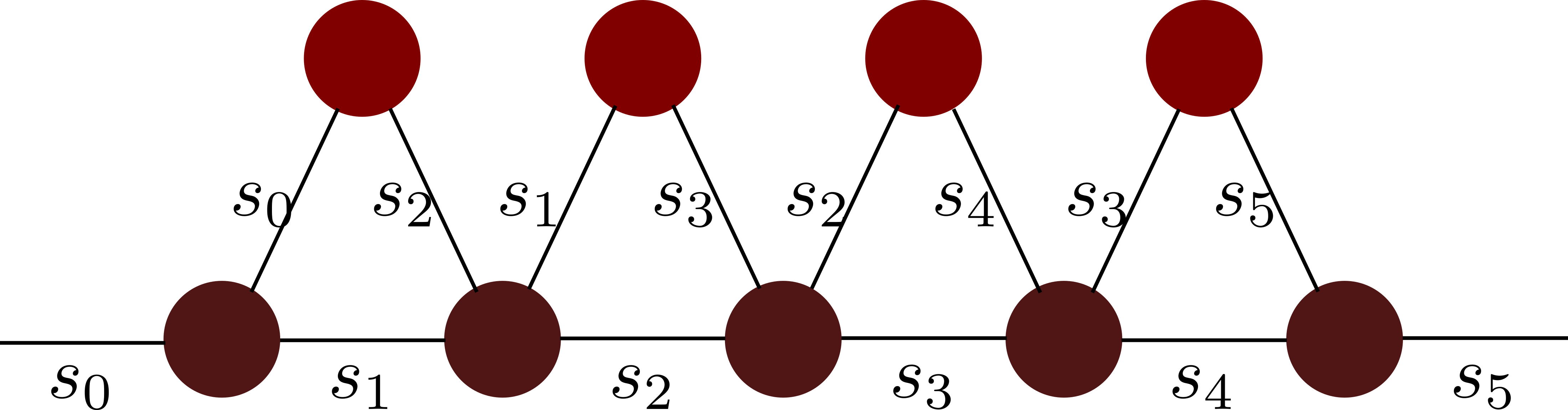
Figure 2: Diagram for $P^{(2)}$ for a $5$-step propagation. The darker circles which form the base represent the $\mathbb{K}$ tensors. The comparatively lighter red circles forming the second layer represent the $I^{(2)}$ tensors. The labels of the non-horizontal indices have been reverted back to the $s$ coordinate by using the $\delta$ function relations in Eq. (12), Eq. (13) and Eq. (14).

The pattern for inclusion of the rest of the non-local interactions is quite similar. Note that in Fig. 2, if we did the same “trick” of duplicating and flipping the order of the inputs, in the next layer indices that differ by three time points, like $s_{0}$ and $s_{3}$, $s_{1}$ and $s_{4}$, are going to be adjacent. Hence, this can now be multiplied by $I^{(3)}_{s_{j-3},s_{j}}$. Continuing like this, we can complete the network. The diagram is shown in Fig. 3 [33], these augmented tensors are going to be written as $\mathbb{K}$, $\mathbb{I}^{(2)}$, …. The tensor network shown in Fig. 3, which we will conventionally denote by $P^{(\infty)}$, represents the final Green’s function for the propagation of the system RDM having incorporated the non-local influence from the environment. So, $\rho(t)=P^{(\infty)}\rho(0)$.

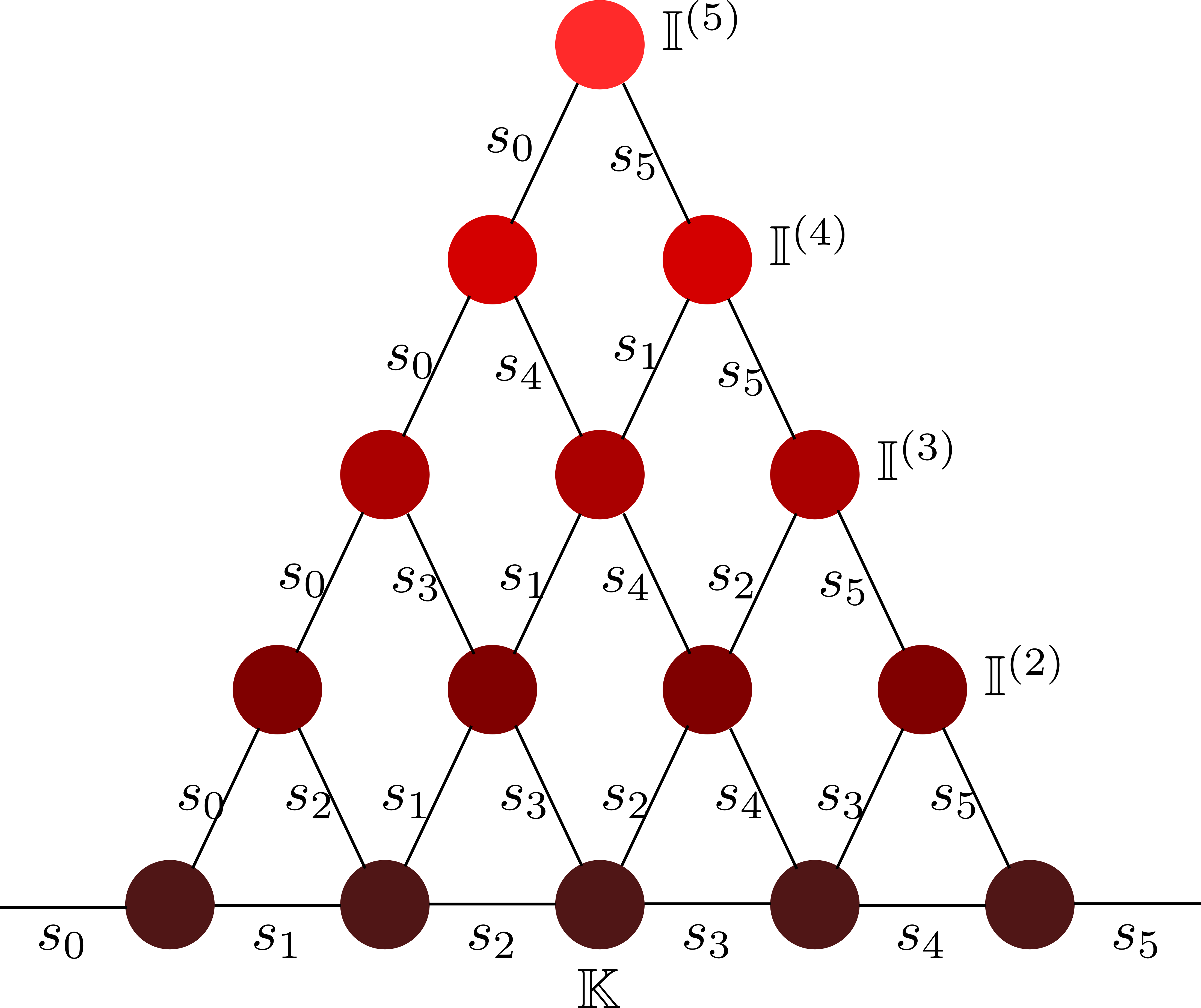
Figure 3: Diagram for the final Green’s function for a $5$-step propagation. Dark brown circles represent the $\mathbb{K}$ tensors. The various red circles represent the $\mathbb{I}$ tensors for different separations. The lighter reds show a larger separation between interacting time-points.

If the system is defined to have $D$ states, then in Fig. 3, all the indices have $D^{2}$ dimensionality corresponding to each of the possible combination of forward-backward states. However, this is not optimal. Notice that the influence functional tensors, $I^{(\alpha)}_{s_{k-\alpha},s_{k}}$ for a time difference of $\alpha$, depends only on the “difference” coordinate, $\Delta s_{k}=s_{k}^{+}-s_{k}^{-}$ of the latter time point. So, currently, we are carrying over more information than we need to.

To take care of this redundancy, we need to redefine the $\mathbb{K}$ tensors to not just duplicate the input indices, but to project the “latter” index onto its difference coordinates as follows:

$$\mathbb{\tilde{K}}^{l_{N-1}}_{s_{N-1},s_{N}} =K_{s_{N-1},s_{N}}\delta_{s^{+}_{N}-s^{-}_{N},l_{N-1}}$$ ((16))

$$\mathbb{\tilde{K}}^{l_{j-1},r_{j}}_{s_{j-1},s_{j}} =K_{s_{j-1},s_{j}}\delta_{s^{+}_{j}-s^{-}_{j},l_{j-1}}\delta_{s_{j-1},r_{j}}\quad\text{if }j\neq 1\text{ and }N.$$ ((17))

Notice that the upper-right output indices in the diagrams remain exactly the same. Only the upper-left output index of $\mathbb{K}$ changes. Therefore, the tensor $\mathbb{K}^{r_{1}}_{s_{0},s_{1}}$ remains unchanged. The dimensionality of the “$l$” indices is the number of unique values of $\Delta s=s^{+}-s^{-}$ that the system can have. For a general $D$-level system, this value is $B=D^{2}-D+1$ instead of $D^{2}$, however the actual symmetries present in the system might reduce this even further. Finally, the influence functional tensors have to be changed to be consistent, viz. $\mathbb{\tilde{I}}^{(\alpha)}_{s_{k-\alpha},\Delta s_{k}}=\exp\left(-\frac{1}{\hbar}\Delta s_{k}(\eta_{k,(k-\alpha)}s^{+}_{k-\alpha}-\eta^{*}_{k,(k-\alpha)}s^{-}_{k-\alpha})\right)$. Even with these changes, the basic topology of the network remains the same. The new network with the different dimensions is shown in Fig. 4.

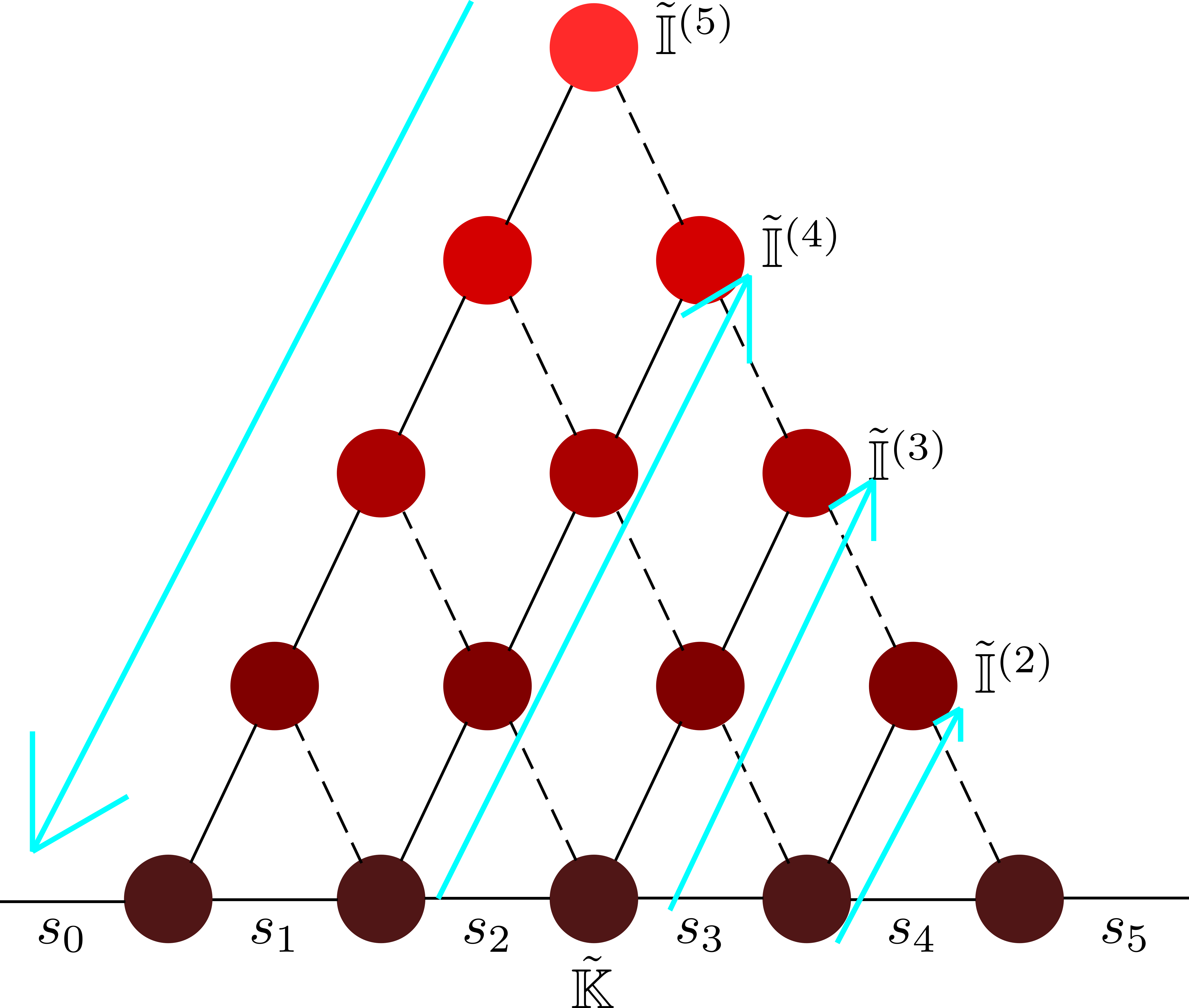
Figure 4: Optimized diagram for the final Green’s function for a $5$-step propagation. Dashed lines have dimension $B$, and solid lines carry dimension $D^{2}$. Cyan arrows show the order of contraction.

Having discussed the tensor network, now let us turn to the job of contracting it. Typically, many tensor networks are constructed using singular value decomposition (SVD) and evaluated via the truncation of the singular values [21, 24]. The PCTNPI network is constructed without resorting to any SVD calculations and consequently “exact.” The goal now is to find an optimal contraction scheme that preserves this “exactness.” The storage cost, $S$, is also evaluated at the end of every step. The canonical contraction order that we discuss below has been marked out in cyan arrows in Fig. 4. For a simulation with $N$ time steps:

1. Start with $\tilde{\mathbb{I}}^{(N)}_{s_{0},s_{N}}$ and contract it with $\tilde{\mathbb{I}}^{(N-1)}_{s_{0},s_{N-1}}$. $S=D^{2}B^{2}$.
   

2. Multiply by $\tilde{\mathbb{I}}^{(N-2)}_{s_{0},s_{N-2}}$. $S=D^{2}B^{3}$.

3. Multiply all $\tilde{\mathbb{I}}^{(\alpha)}_{s_{0},s_{\alpha}}$ followed by $\mathbb{\tilde{K}}_{s_{0},s_{1}}\rho_{s_{0}}$. At this stage the storage cost is $S=D^{2}B^{N-1}$.

4. Contract the second edge sequentially, starting from $\mathbb{\tilde{K}}_{s_{1},s_{2}}$. $S=(D^{2})^{2}B^{N-2}$.

5. While contracting the remaining $N-3$ tensors on the second edge, the storage cost remains constant at $S=(D^{2})^{2}B^{N-2}$.

6. Lastly, the topmost tensor on the second edge needs to be contracted. The storage drops to $S=D^{2}B^{N-2}$.

7. Continuing in the same fashion, the storage requirements of contracting the internal tensors of the $j$^th edge is $S=(D^{2})^{2}B^{N-j}$ when $j<N$.

8. After contracting the final tensor on the $j$^th edge, the storage drops to $S=D^{2}B^{N-j}$.

9. Finally, the last tensor, $\mathbb{\tilde{K}}_{s_{N-1},s_{N}}$ is contracted.

In the above contraction scheme, we multiply the initial condition, $\rho_{s_{0}}$, and get the final RDM. While this leads to a more efficient algorithm in terms of the storage and computational cost, it is possible to reformulate the scheme in terms of the Green’s function by not involving the initial condition in the contractions and evaluating $P^{(\infty)}$. An in-depth analysis of the memory and computational cost is given in Appendix A. Of course, the storage requirement grows to a maximum of $(D^{2})^{2}B^{N-2}$ before decreasing continuously. This naïve contraction scheme does not solve the problem of storage. Still, as would be illustrated in Sec. III, PCTNPI outperforms both traditional iterative quasi-adiabatic propagator path integrals (QuAPI) [31, 32], and iterative blip summed path integral (BSPI) [17, 18], when used without path filtration, in the memory lengths that can be accessed without any sort of filtration. In a future work, filtration schemes on top of PCTNPI would be introduced that can not only deal with this problem, but would also avoid the construction and storage of the full tensor. The focus of this paper is however on the tensor network and its performance in the most naïve implementation.

It is well-known that the non-local memory of the influence functional dies away with the distance between the points, allowing for a truncation of memory. This idea is commonly used both in Nakajima-Zwanzig generalized quantum master equations [34, 35, 36] and iterative QuAPI [31, 32]. In the framework of PCTNPI, the length of the non-Markovian memory is equal to the depth of the resultant network. The topmost tensor encodes the interaction between the most distant points, while the bottom most tensor captures the Markovian interactions coming through the propagator and the $I^{(1)}$ terms.

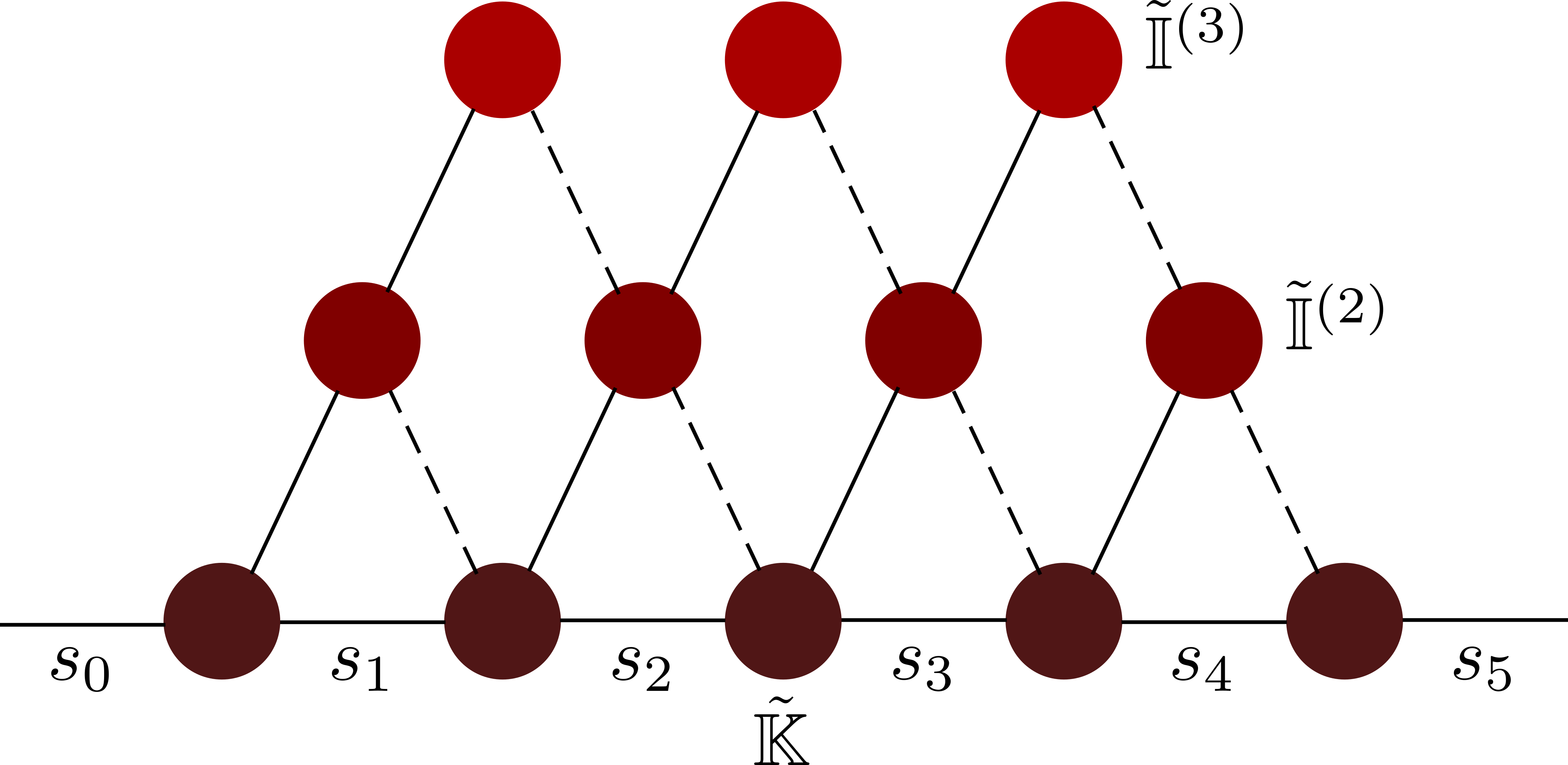
Figure 5: Diagram for the final Green function for a 5-step propagation with memory length $L=3$.

At two time-steps of memory, that is $L=2$, we basically get Fig. 2. In Fig. 5, we show the structure of the network for a 5-step propagation with $L=3$. Because $s_{0}$ does not interact with $s_{4}$ or $s_{5}$, it is not necessary to store and evaluate the full diagram at once, but it can be built iteratively. The first edge, corresponding to interactions with $s_{0}$ is contracted, and multiplied by the second edge, using the canonical contraction scheme discussed previously. As soon as this is done, the storage of the first edge can be freed, and the third edge can be contracted. This iteration scheme turns out to be identical to the iteration scheme in iterative QuAPI. The first steps of the iteration algorithm is pictorally outlined in Fig. 6.

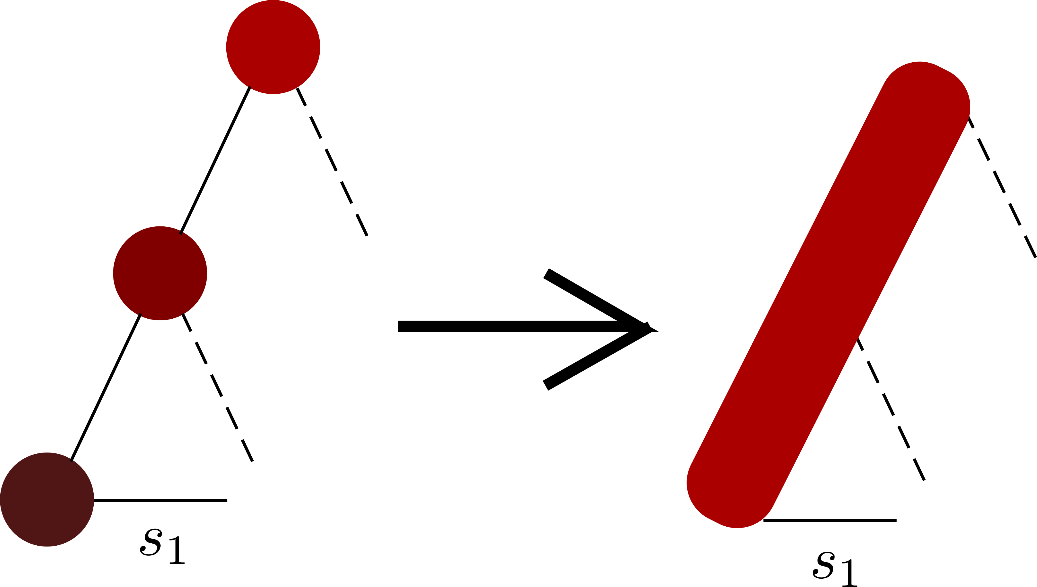
(a) Contract all influence functionals with $s_{0}$.

(b) Contract result with all influence functionals with $s_{1}$. Notice that the external index with $s_{1}$ from the previous step has been contracted out and now the bottom-most external index is $s_{2}$.

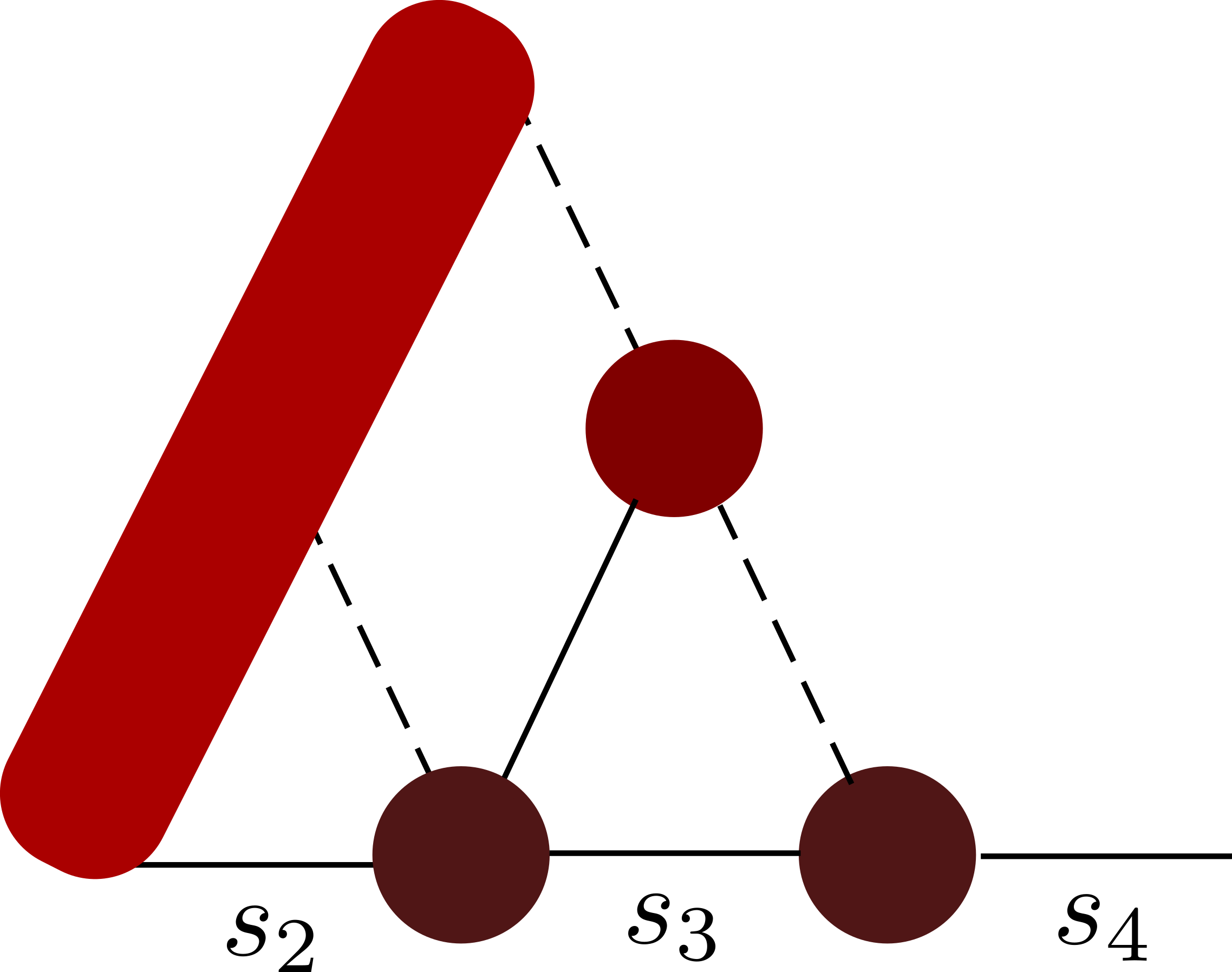
(c) Contract result with remaining terms to get RDM.

Figure 6: First steps of algorithm for iteration. The basic contractions are done in the same way as described for the full path part.

Makri [17] has shown that it is possible to think of the memory as arising from two different causes. The influence functional $F$ can be rewritten in terms of the real and imaginary parts of the $\eta$-coefficients as:

$$F[\{s^{\pm}_{j}\}] =e^{-\frac{1}{\hbar}\sum_{k}\Delta s_{k}\sum_{k^{\prime}\leq k}(\real\eta_{kk^{\prime}}\Delta s_{k^{\prime}}-2i\imaginary\eta_{kk^{\prime}}\bar{s}_{k^{\prime}})}$$ ((18))

where $\Delta s_{k}=s_{k}^{+}-s_{k}^{-}$ and $\bar{s}_{k}=\tfrac{1}{2}(s^{+}_{k}+s^{-}_{k})$. The part of the influence functional that arises from $\real\eta_{kk^{\prime}}$ is called the classical decoherence factor. It corresponds to stimulated phonon absorption and emission [37]. This can also be obtained through classical trajectory-simulations and reference propagators [38] in a Markovian manner. All effects of temperature is captured in the classical decoherence term. The term with the $\imaginary\eta_{kk^{\prime}}$ is the back-reaction that leads to quantum decoherence. This part of the memory is truly non-local and temperature independent.

As a cheap approximation to the dynamics, it is possible to do a simulation with classical decoherence, that would become increasing accurate as the temperature of the simulation rises. In this, the full $\eta_{kk^{\prime}}$ coefficients are used only when $k=k^{\prime}$ or $k=k^{\prime}+1$, and otherwise the imaginary part of $\eta_{kk^{\prime}}$ is ignored. (Actually, the true expressions for classical decoherence would include the full $\eta_{kk^{\prime}}$ coefficients only when $k=k^{\prime}$ and the real part otherwise. In PCTNPI, we can include the case of $k=k^{\prime}+1$ as well at the same storage and computational cost.) Effectively, we are modifying the $I^{(\alpha)}_{s_{k^{\prime}},s_{k}}$ operators to be $\exp\left(-1/\hbar\real(\eta_{kk^{\prime}})\Delta s_{k}\Delta s_{k^{\prime}}\right)$ when $\alpha=k-k^{\prime}\geq 2$. Just like before when the $s_{k}$ lines carried unnecessary information, now the $s_{k^{\prime}}$ lines carry more information than they need to. We only need to know about $\Delta s_{k^{\prime}}$. Thus we can make the required changes to the dimensionality of the indices by putting in the corresponding projector operators in the $\mathbb{K}$ tensors, thereby reducing the cost of computation even further. The network for the classical decoherence simulations would have exactly the same structure as Fig. 3 with all edges except the base ones being $B$ dimensional. This approximation is especially accurate at short times.

III Results

As illustrative examples, we apply PCTNPI to a two-level systems (TLS) coupled bilinearly to a dissipative environment:

$$\hat{H}_{0} =\epsilon\hat{\sigma}_{z}-\hbar\Omega\hat{\sigma}_{x}$$ ((19))

The dissipative environment is chosen to be defined by Ohmic model spectral densities, which are especially useful in modeling the low frequency ro-translational modes. We use the very common Ohmic form with an exponential cutoff,

$$J(\omega)=\frac{\pi}{2}\hbar\xi\omega\exp\left(-\frac{\omega}{\omega_{c}}\right)$$ ((20))

where $\xi$ is the dimensionless Kondo parameter and $\omega_{c}$ is the characteristic cutoff frequency and the Ohmic form with a Drude cutoff,

$$J(\omega)=\kappa\omega_{c}\frac{\omega}{\omega^{2}+\omega_{c}^{2}}$$ ((21))

where $\kappa$ is a measure of the coupling strength. Generally these model spectral densities are often thought to be fully characterized by a reorganization energy

$$\lambda=\frac{2}{\pi}\int_{-\infty}^{\infty}\frac{J(\omega)}{\omega}\differential{\omega}$$ ((22))

and the cutoff frequency, $\omega_{c}$. The reorganization energies for the exponential and the drude cutoff spectral densities are as listed below:

$$\lambda_{\text{Exp}} =2\xi\omega_{c}$$ ((23))

$$\lambda_{\text{Drude}} =2\kappa.$$ ((24))

As we demonstrate through the examples, though the reorganization energy and the cutoff frequency are same, the exact dynamics of the reduced density matrix is highly dependent on the form of the “decay function.”

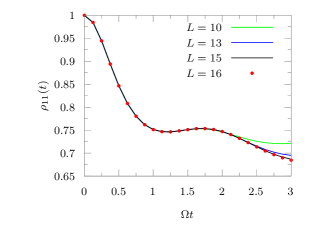
(a) Convergence with respect to memory length, $L$.

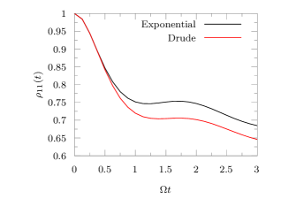
(b) Comparison between spectral densities with exponential and Drude decay functions.

Figure 7: Dynamics of a symmetric TLS interacting with a bath with $\lambda=2,\omega_{c}=\Omega$ at an inverse temperature $\hbar\Omega\beta=1$.

Consider a symmetric TLS ($\epsilon=0$) and $\Omega=1$ interacting strongly ($\xi=2$) with a sluggish bath ($\omega_{c}=\Omega$) initially localized on the populated system state $1$. The bath has a reorganization energy of $\lambda=4$ and is held at an inverse temperature of $\hbar\Omega\beta=1$. The dynamics was converged at $\Delta t=0.125$, and a memory length $L=16$. The convergence is shown in Fig. 7 (a) for an Ohmic bath with an exponential decay. Full quantum-classical simulations for this parameter is available [39]. If the Drude form of decay is used, the dynamics changes quite significantly. The comparison between the dynamics arising from the two spectral densities is shown in Fig. 7 (b).

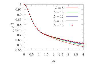
(a) Spectral density with exponential decay functions

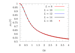
(b) Spectral density with Drude decay functions

Figure 8: Convergence with respect to memory length for the spectral density with an exponential cutoff.

Next, consider a case where not only is the dynamics different between the two different decay functions, but the converged non-Markovian memory length is different as well. The dynamics of the same TLS as above ($\epsilon=0,\Omega=1$) is now simulated in a bath with the reorganization energy $\lambda=8$ and a characteristics cutoff frequency $\omega_{c}=5$. The bath is equilibrated at an inverse temperature of $\hbar\Omega\beta=5$. The time-step is converged at $\Omega\Delta t=0.125$. The convergence of the dynamics of the reduced density matrix on changing the memory length, $L$, is shown in Fig. 8. While the memory length for the exponential decay function spectral density is quite close to convergence at $L=14$, for the Drude spectral function, it converges at $L=10$.

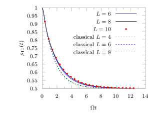
Figure 9: Comparison between the classical and full memory calculations for a strongly coupled high temperature bath.

In Fig. 9, we consider a TLS coupled to a strongly coupled Ohmic bath with an exponential cutoff ($\xi=1.2$, $\omega_{c}=2.5\Omega$) equilibrated at a high temperature $\hbar\Omega\beta=0.2$. The converged time step is $\Delta t=0.125$. The classical memory calculations converge at a comparatively lower memory length, $L$ and agree quite well with the full simulations at short times. Though at intermediate and long times, the classical decoherence dynamics differs from the true dynamics, this can often be enough for estimating timescales of processes, especially using rate theory [40, 41, 42, 43].

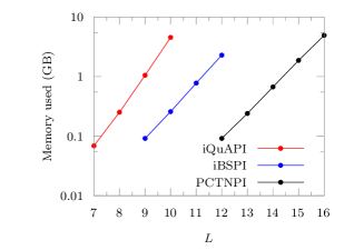
(a) Plot of memory requirements with respect to memory length for different methods.

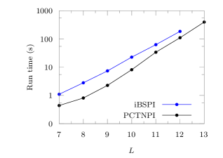
(b) Plot of execution times with respect to memory length for different methods.

Figure 10: Comparison of PCTNPI with other methods. Note that while the memory used is independent of machine, but the execution time is not.

Next, the storage requirements of PCTNPI is compared with that of iterative QuAPI and iterative BSPI in Fig. 10 (a). To keep the comparisons fair, the iQuAPI and iBSPI methods were run without any path filtering. It is quite clear from the plot that the scaling of PCTNPI is essentially “like” that of iBSPI, i.e. for a TLS, $3^{L}$ scaling for iBSPI and PCTNPI vs $4^{L}$ scaling of iQuAPI. However, the prefactor is much smaller, allowing us to access much longer memories with limited resources. In fact, this difference in the prefactor would grow with the dimensionality of the quantum system. In iBSPI, there would be $3^{L}$ paths for a memory length of $L$, but the storage is more than just a number corresponding to each path. It stores a small dimensional matrix for each path. This is the cause of the larger prefactor.

A comparison of the run times of PCTNPI with respect to iBSPI without any filtration for a simulation of 100 time steps is presented in Fig. 10 (b). A laptop with Intel® Core^TM i5-4200U CPU with a clock speed of 1.60GHz was used for these benchmark calculations. These measurements are not going to be consistent with similar benchmarks run on other machines, but the basic trends would continue to hold. The PCTNPI algorithm is built on top of ITensor and automatically uses parallel BLAS and LAPACK wherever possible. There is no standard iBSPI code. The iBSPI program used for these benchmarks was manually parallelized with OpenMP loop parallelization.

As a final example, consider a molecular wire described by the tight-binding Hamiltonian involving $N$ sites:

$$\hat{H}_{0} =\sum_{1\leq j\leq N}\epsilon_{j}\outerproduct{\sigma_{j}}{\sigma_{j}}-\hbar V\sum_{1\leq j<N}(\outerproduct{\sigma_{j}}{\sigma_{j+1}}+\outerproduct{\sigma_{j+1}}{\sigma_{j}}).$$ ((25))

The site energy of the $j$^th site is $\epsilon_{j}$ and the nearest neighbor couplings are $V$. The sites are separated by unit distance such that $\ket{\sigma_{j}}$ are eigenstates of the position operator, $\hat{s}\ket{\sigma_{j}}=(j-1)\ket{\sigma_{j}}$. The site energy of all but the first site is chosen to be zero $\epsilon_{j}=0$ for $j\neq 1$ and $\epsilon_{1}=1$. The intersite coupling is chosen to be $V=0.025$ [44].

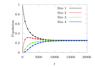
Figure 11: Population dynamics corresponding to an initially populated first site. Lines: full simulations, markers: classical memory simulations. For full decoherence, $L=6$; for classical decoherence, $L=4$.

The computational cost grows exponentially with the number of sites. To test the efficiency of the basic contraction scheme outlined here, we use a system with $N=4$ sites. The bath is characterized by an Ohmic spectral density with an exponential cutoff, Eq. (20) with $\omega_{c}=4$ and $\xi=0.12$ [24] equilibrated at an inverse temperature of $\beta=0.1$. As discussed in Sec. II, the scaling of the algorithm would go as $B<D^{2}$. The symmetry of the Hamiltonian in this case ensures that the number of unique values of $\Delta s$, $B=7$ for this 4 state system, which is even less than the $D^{2}-D+1$ for a completely general Hamiltonian. The population dynamics of all the states is shown in Fig. 11. An initial state with only the first site populated was used. Because of the high temperature of the bath, the classical decoherence simulation produces practically identical dynamics but converges at a smaller memory length $L$.

IV Conclusion

A novel tensor network is introduced to perform path integral calculations involving the Feynman-Vernon influence functional. This pairwise connected tensor network path integral (PCTNPI) captures the pairwise interaction structure of influence functional. PCTNPI can be contracted efficiently, and minimizes the storage requirements as far as possible without resorting to various path filtration algorithms. Iterative decomposition of the memory is also possible in an elegant manner. Comparisons between PCTNPI and iQuAPI and iBSPI show the scaling of memory requirements of PCTNPI to be similar to iBSPI, but much smaller.

PCTNPI provides an alternative to the MPS representation [21, 24], serving as a small step in further elucidating the deep relation between tensor networks and path integrals. While no path filtration scheme has been developed, PCTNPI is already quite useable. It can easily incorporate classical trajectories through harmonic backreaction quantum-classical path integrals [37] thereby making it possible to include anharmonic effects of the environment in an approximate manner without any additional cost. Additionally, harmonic backreaction also leads to an increase in the converged time-step and a decrease in the effective memory length such that some ultrafast reactions can be simulated directly. Taking advantage of the extended memories that are accessible with PCTNPI, the combined method would be able to simulate systems with strongly coupled sluggish realistic solvents with high reorganization energy. This promises to be a fruitful avenue of research in terms of applications to electron and proton transfer reactions.

Algorithms based on MPS representations of the augmented reduced density tensor [21] or of the path-dependent Green’s function [24] can be thought of as particular optimized re-factorizations of the PCTNPI network. We have demonstrated the viability of evaluating PCTNPI in a brute force manner compared to other methods. This suggests that using the PCTNPI network directly to generate other optimized representations might also lead to novel methods.

While ideas of path filtration were not a consideration of the present paper, schemes based on the singular value decomposition (SVD) can be incorporated with PCTNPI, leading to a method that significantly reduces the storage, since the full tensor would not need to be computed and stored. This development would be discussed in a future publication.

Appendix A Cost of Contraction

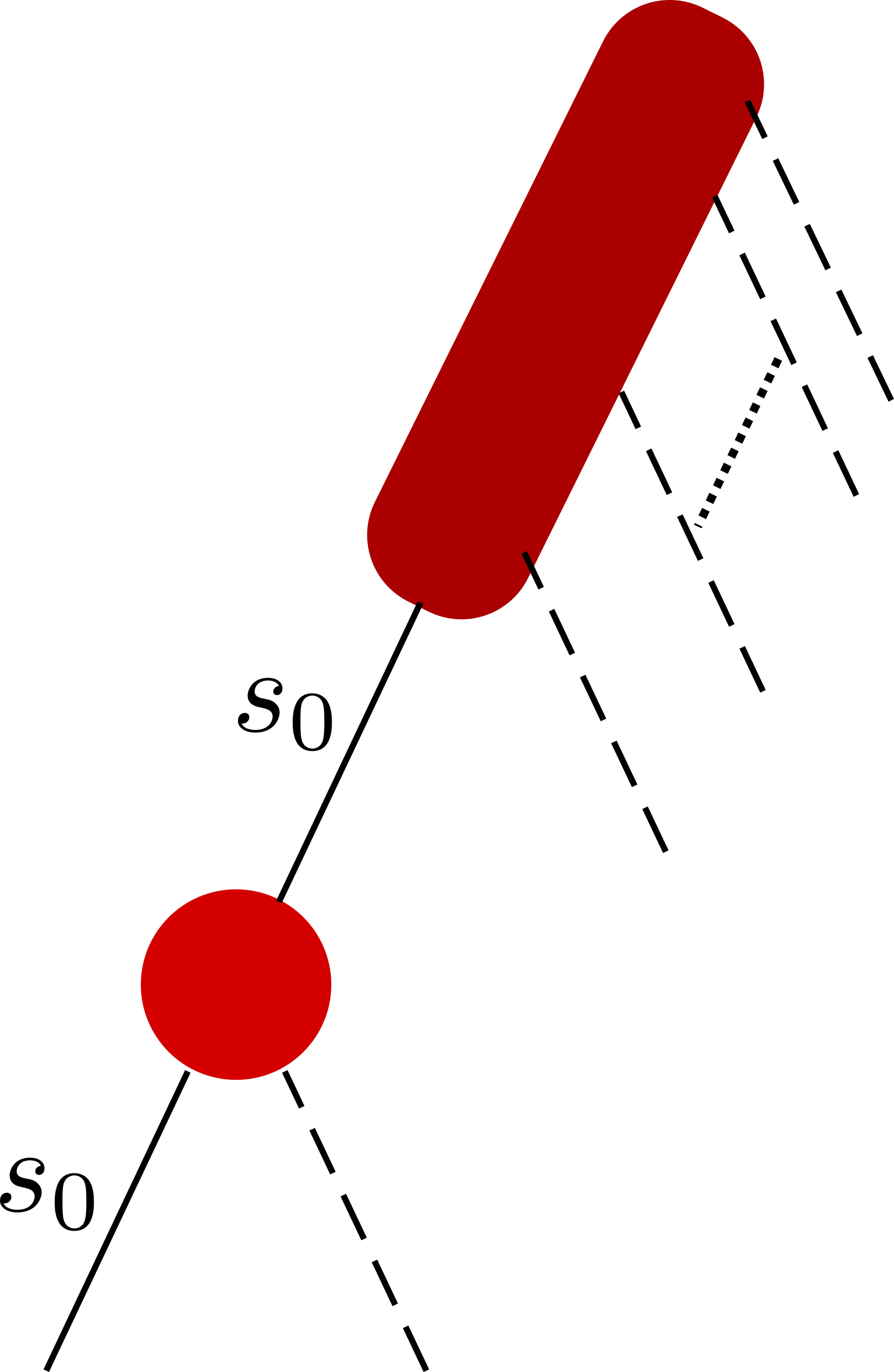
(a) Contraction of internal tensor along the left edge ($j\geq 2$). $C=(D^{2})^{2}B^{N-j+1}$. $S=D^{2}B^{N-j+1}$.

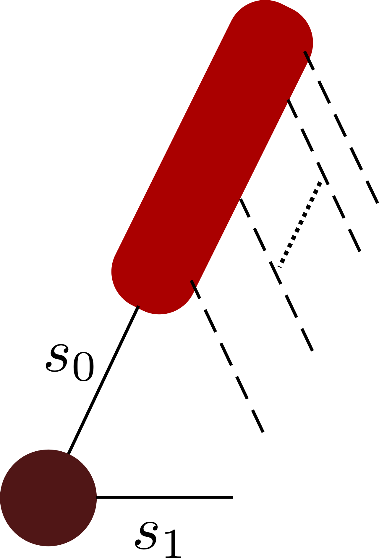
(b) Contraction of $\tilde{\mathbb{K}}_{s_{0},s_{1}}\rho_{s_{0}}$. $C=(D^{2})^{2}B^{N-1}.$ $S=D^{2}B^{N-1}$.

Figure 12: Contraction along the left edge of the triangle. Dashed lines show the $B$ dimensional indices, and solid lines show the $D^{2}$ dimensional indices.

Consider the tensor network corresponding to a full path simulation spanning $N$ time-steps. To calculate the cost of contraction, the left “edge” of the triangular network is first considered. Consider contracting $\tilde{\mathbb{I}}^{(j)}_{s_{0},s_{j}}$, for $j\geq 2$, with two $D^{2}$ indices and one $B$ index, as schematically indicated in Fig. 12 (a). The part that has already been contracted has one $D^{2}$ index and $(N-j)$ $B$ indices. Therefore, the cost of contraction is $(D^{2})^{2}B^{N-j+1}$. The space requirement at this stage is $D^{2}B^{N-j+1}$. To finish the contraction of the left-most edge of the triangle, we need to multiply by $\tilde{\mathbb{K}}_{s_{0},s_{1}}\rho_{s_{0}}$ leading to the tensor network shown in Fig. 12 (b). The resultant tensor does not have a index corresponding to $s_{0}$ because that has been traced over. The computational cost of this step is $C=(D^{2})^{2}B^{N-1}$ and the storage becomes $S=D^{2}B^{N-1}$.

Now, the second parallel edge is to be contracted. This step however is started from the bottom, i.e. from $\tilde{\mathbb{K}}_{s_{1},s_{2}}$. The first contraction, shown in Fig. 13 (a), is the most costly step in the entire algorithm. The computational cost of this step is $C=(D^{2})^{3}B^{N-1}$ and the storage requirement increases to $S=(D^{2})^{2}B^{N-2}$. Continuing with the other intermediate tensors of the first parallel edge, notice that the cost of contraction remains constant at $C=(D^{2})^{3}B^{N-1}$ and the space required remains constant at $S=(D^{2})^{2}B^{N-2}$. Finally, the last, top-most tensor of this edge is to be contracted. This is illustrated in Fig. 13 (b). The computational cost is $C=(D^{2})^{2}B^{N-1}$. The storage cost now drops to $S=D^{2}B^{N-2}$.

(a) Contracting the first tensor of the next parallel edge. $C=(D^{2})^{3}B^{N-1}$. $S=(D^{2})^{2}B^{N-2}$.

(b) Contracting the last tensor of the next parallel edge. $C=(D^{2})^{2}B^{N-1}$. $S=D^{2}B^{N-2}$.

Figure 13: Contraction along an intermediate edge, say the one next to the left-most edge.

Now, consider contracting a general diagonal edge, say the $j$^th one. The resultant tensor from the previous contraction has one $D^{2}$ index and $N-j+1$ $B$ indices. Contracting the $\tilde{\mathbb{K}}$ tensor leads to a tensor with two $D^{2}$ indices and $(N-j)$ $B$ indices. The cost of this contraction is $C=(D^{2})^{3}B^{N-j+1}$ and the storage is $S=(D^{2})^{2}B^{N-j}$. For all the intermediate tensors at this stage, once again both the computational costs and the storage costs remain the same. On contracting the last tensor of this diagonal, the storage drops to $S=D^{2}B^{N-j}$.

Below we list the total computational cost for contracting each of the “parallel” edges. The edge number is given as the subscript.

$$C_{1} =(D^{2})^{2}B^{N-1}+\sum_{j=2}^{N-1}(D^{2})^{2}B^{N-j+1}$$

$$=(D^{2})^{2}\left(B^{N-1}+\frac{B^{2}(B^{N-2}-1)}{B-1}\right)$$ ((26))

$$C_{j} =(D^{2})^{2}B^{N-j+1}\left(1+(N-j)D^{2}\right),\quad 2\leq j\leq N$$ ((27))

The prefactor of the computational and storage costs is lower for classical decoherence simulations: It goes from a power of $D^{2}$ to the corresponding power of $B$. It is clear that the complexity of the entire contraction goes as $\mathcal{O}\left(B^{N-1}\right)$ and the peak storage requirement is $\mathcal{O}\left(B^{N-2}\right)$.

References

- White [1992] S. R. White, Density matrix formulation for quantum renormalization groups, Phys. Rev. Lett. 69, 2863 (1992).
- Schollwöck [2005] U. Schollwöck, The density-matrix renormalization group, Rev. Mod. Phys. 77, 259 (2005).
- Schollwöck [2011a] U. Schollwöck, The density-matrix renormalization group in the age of matrix product states, Ann. Phys. (N. Y). 326, 96 (2011a).
- Schollwöck [2011b] U. Schollwöck, The density-matrix renormalization group: A short introduction, Philos. Trans. R. Soc. A Math. Phys. Eng. Sci. 369, 2643 (2011b).
- Beck et al. [2000] M. H. Beck, A. Jäckle, G. A. Worth, and H.-D. Meyer, The multiconfiguration time-dependent Hartree (MCTDH) method: A highly efficient algorithm for propagating wavepackets, Phys. Rep. 324, 1 (2000).
- Wang and Thoss [2003] H. Wang and M. Thoss, Multilayer formulation of the multiconfiguration time-dependent Hartree theory, J. Chem. Phys. 119, 1289 (2003).
- Schulze et al. [2016] J. Schulze, M. F. Shibl, M. J. Al-Marri, and O. Kühn, Multi-layer multi-configuration time-dependent Hartree (ML-MCTDH) approach to the correlated exciton-vibrational dynamics in the FMO complex, J. Chem. Phys. 144, 185101 (2016).
- Shibl et al. [2017] M. F. Shibl, J. Schulze, M. J. Al-Marri, and O. Kühn, Multilayer-MCTDH approach to the energy transfer dynamics in the LH2 antenna complex, J. Phys. B At. Mol. Opt. Phys. 50, 184001 (2017).
- Orús [2014] R. Orús, A practical introduction to tensor networks: Matrix product states and projected entangled pair states, Ann. Phys. (N. Y). 349, 117 (2014).
- Vidal [2007] G. Vidal, Entanglement Renormalization, Phys. Rev. Lett. 99, 220405 (2007).
- Vidal [2008] G. Vidal, Class of quantum Many-Body states that can be efficiently simulated, Phys. Rev. Lett. 101, 1 (2008).
- White and Feiguin [2004] S. R. White and A. E. Feiguin, Real-Time Evolution Using the Density Matrix Renormalization Group, Phys. Rev. Lett. 93, 076401 (2004).
- Ma et al. [2018] H. Ma, Z. Luo, and Y. Yao, The time-dependent density matrix renormalisation group method, Mol. Phys. 116, 854 (2018).
- Makri [1999] N. Makri, The Linear Response Approximation and Its Lowest Order Corrections: An Influence Functional Approach, J. Phys. Chem. B 103, 2823 (1999).
- Feynman and Vernon [1963] R. P. Feynman and F. L. Vernon, The theory of a general quantum system interacting with a linear dissipative system, Ann. Phys. (N. Y). 24, 118 (1963).
- Makri [2012] N. Makri, Path integral renormalization for quantum dissipative dynamics with multiple timescales, Mol. Phys. 110, 1001 (2012).
- Makri [2014a] N. Makri, Exploiting classical decoherence in dissipative quantum dynamics: Memory, phonon emission, and the blip sum, Chem. Phys. Lett. 593, 93 (2014a).
- Makri [2014b] N. Makri, Blip decomposition of the path integral: Exponential acceleration of real-time calculations on quantum dissipative systems, J. Chem. Phys. 141, 134117 (2014b).
- Makri [2020a] N. Makri, Small matrix disentanglement of the path integral: Overcoming the exponential tensor scaling with memory length, J. Chem. Phys. 152, 041104 (2020a).
- Makri [2020b] N. Makri, Small Matrix Path Integral for System-Bath Dynamics, J. Chem. Theory Comput. 16, 4038 (2020b).
- Strathearn et al. [2018] A. Strathearn, P. Kirton, D. Kilda, J. Keeling, and B. W. Lovett, Efficient non-Markovian quantum dynamics using time-evolving matrix product operators, Nat. Commun. 9, 1 (2018).
- Guo et al. [2020] C. Guo, K. Modi, and D. Poletti, Tensor-network-based machine learning of non-Markovian quantum processes, Phys. Rev. A 102, 1 (2020).
- Fux et al. [2021] G. E. Fux, E. P. Butler, P. R. Eastham, B. W. Lovett, and J. Keeling, Efficient Exploration of Hamiltonian Parameter Space for Optimal Control of Non-Markovian Open Quantum Systems, Phys. Rev. Lett. 126, 200401 (2021).
- Bose and Walters [tted] A. Bose and P. L. Walters, A tensor network representation of path integrals: Implementation and analysis, J. Chem. Theory Comput. (submitted), arXiv:2106.12523 [physics.chem-ph] .
- [25] ITensor Library (version 3.0.0), ITensor Libr. (version 3.0.0) https://itensor.org.
- Caldeira and Leggett [1983a] A. O. Caldeira and A. J. Leggett, Path integral approach to quantum Brownian motion, Phys. A Stat. Mech. its Appl. 121, 587 (1983a).
- Caldeira and Leggett [1983b] A. O. Caldeira and A. J. Leggett, Quantum tunnelling in a dissipative system, Ann. Phys. (N. Y). 149, 374 (1983b).
- Leggett et al. [1987] A. J. Leggett, S. Chakravarty, A. T. Dorsey, M. P. A. Fisher, A. Garg, and W. Zwerger, Dynamics of the dissipative two-state system, Rev. Mod. Phys. 59, 1 (1987).
- Makri [1992] N. Makri, Improved Feynman propagators on a grid and non-adiabatic corrections within the path integral framework, Chem. Phys. Lett. 193, 435 (1992).
- Leppäkangas et al. [2018] J. Leppäkangas, J. Braumüller, M. Hauck, J. M. Reiner, I. Schwenk, S. Zanker, L. Fritz, A. V. Ustinov, M. Weides, and M. Marthaler, Quantum simulation of the spin-boson model with a microwave circuit, Phys. Rev. A 97, 10.1103/PhysRevA.97.052321 (2018).
- Makri and Makarov [1995a] N. Makri and D. E. Makarov, Tensor propagator for iterative quantum time evolution of reduced density matrices. I. Theory, J. Chem. Phys. 102, 4600 (1995a).
- Makri and Makarov [1995b] N. Makri and D. E. Makarov, Tensor propagator for iterative quantum time evolution of reduced density matrices. II. Numerical methodology, J. Chem. Phys. 102, 4611 (1995b).
- Strathearn [2020] A. Strathearn, Modelling Non-Markovian Quantum Systems Using Tensor Networks, Ph.D. thesis, University of St. Adrews (2020).
- Nakajima [1958] S. Nakajima, On Quantum Theory of Transport Phenomena, Prog. Theor. Phys. 21, 659 (1958).
- Zwanzig [1960] R. Zwanzig, Ensemble method in the theory of irreversibility, J. Chem. Phys. 33, 1338 (1960).
- Shi and Geva [2003] Q. Shi and E. Geva, A new approach to calculating the memory kernel of the generalized quantum master equation for an arbitrary system–bath coupling, J. Chem. Phys. 119, 12063 (2003).
- Wang and Makri [2019] F. Wang and N. Makri, Quantum-classical path integral with a harmonic treatment of the back-reaction, J. Chem. Phys. 150, 184102 (2019).
- Banerjee and Makri [2013] T. Banerjee and N. Makri, Quantum-classical path integral with self-consistent solvent-driven reference propagators, J. Phys. Chem. B 117, 13357 (2013).
- Walters and Makri [2016] P. L. Walters and N. Makri, Iterative quantum-classical path integral with dynamically consistent state hopping, J. Chem. Phys. 144, 044108 (2016).
- Miller [1974] W. H. Miller, Quantum mechanical transition state theory and a new semiclassical model for reaction rate constants, J. Chem. Phys. 61, 1823 (1974).
- Miller et al. [1983] W. H. Miller, S. D. Schwartz, and J. W. Tromp, Quantum mechanical rate constants for bimolecular reactions, J. Chem. Phys. 79, 4889 (1983).
- Topaler and Makri [1993] M. Topaler and N. Makri, Quasi-adiabatic propagator path integral methods. Exact quantum rate constants for condensed phase reactions, Chem. Phys. Lett. 210, 285 (1993).
- Bose and Makri [2017] A. Bose and N. Makri, Non-equilibrium reactive flux: A unified framework for slow and fast reaction kinetics, J. Chem. Phys. 147, 152723 (2017).
- Lambert and Makri [2012] R. Lambert and N. Makri, Memory propagator matrix for long-time dissipative charge transfer dynamics, Mol. Phys. 110, 1967 (2012).