A second-order accurate numerical scheme for a time-fractional Fokker-Planck equation

Abstract

A time-stepping $L1$ scheme for solving a time fractional Fokker-Planck equation of order $\alpha\in(0,1)$, with a general driving force, is investigated. A stability bound for the semi-discrete solution is obtained for $\alpha\in(1/2,1)$ via a novel and concise approach. Our stability estimate is $\alpha$-robust in the sense that it remains valid in the limiting case where $\alpha$ approaches $1$ (when the model reduces to the classical Fokker-Planck equation), a limit that presents practical importance. Concerning the error analysis, we obtain an optimal second-order accurate estimate for $\alpha\in(1/2,1)$. A time-graded mesh is used to compensate for the singular behavior of the continuous solution near the origin. The $L1$ scheme is associated with a standard spatial Galerkin finite element discretization to numerically support our theoretical contributions. We employ the resulting fully-discrete computable numerical scheme to perform some numerical tests. These tests suggest that the imposed time-graded meshes assumption could be further relaxed, and we observe second-order accuracy even for the case $\alpha\in(0,1/2]$, that is, outside the range covered by the theory.Fractional Fokker-Planck, $L1$ approximations, finite elements, stability and error analysis, graded meshes

1 Introduction

We consider the following time-fractional Fokker-Planck equation (Angstmann et al. (2015))

$$\partial_{t}u(x,t)+\nabla\cdot\Big{(}\partial_{t}^{1-\alpha}\kappa_{\alpha}\nabla u+{{{F}}}\partial_{t}^{1-\alpha}u\Big{)}(x,t)=f(x,t),\quad\mbox{for }x\in\Omega\mbox{ and }0<t<T,$$ (1)

where $\Omega$ is a convex polyhedral domain in $\mathbb{R}^{d}$ ($d\geq 1$). In (1), the diffusivity coefficient $\kappa_{\alpha}$, function of $x$, is assumed uniformly bounded with a lower bound $\kappa_{\min}>0$. The driving force ${{{F}}}:=(F_{1},F_{2},\ldots,F_{d})$ is a vector function of $x$ and $t$, while $f$ is a source term. The functions $\kappa_{\alpha}$, ${{{F}}}$, and $f$ are assumed to be sufficiently regular functions on their respective domains. Further, $\partial_{t}=\partial/\partial t$ is the classical time partial derivative, and the time-fractional derivative $\partial^{1-\alpha}/\partial t$ is taken in the Riemann–Liouville sense, that is

$$\partial_{t}^{1-\alpha}v=\partial_{t}\mathcal{I}^{\alpha}v,~{}~{}\mathcal{I}^{\alpha}v(t)=\int_{0}^{t}\omega_{\alpha}(t-s)v(s)\,ds\mbox{ with }\omega_{\alpha}(t)=\frac{t^{\alpha-1}}{\Gamma(\alpha)},~{}~{}{\rm with}~{}~{}0<\alpha<1.$$

The problem is completed with the initial condition $u(x,0)=u_{0}(x)$, and homogeneous Dirichlet boundary condition $u(x,t)=0$ for $x\in\partial\Omega$ and $0<t<T.$ The well-posedness and regularity properties of problem (1) and more general models were recently investigated in (Le et al. (2019), McLean et al. (2019) and (2020)).

Remark 1.

Assuming $u$ satisfies the regularity assumption in (4) below, the time-stepping stability property and error bound established in this paper for the homogeneous Dirichlet boundary condition remain valid in the case of a zero-flux boundary condition,

$$\partial_{t}^{1-\alpha}\left(\kappa_{\alpha}\frac{\partial u}{\partial n}\right)-({{F}}\cdot{{n}})\,\partial_{t}^{1-\alpha}u=0\quad\mbox{ for }x\in\partial\Omega\mbox{ and }0<t<T,$$ (2)

where ${{n}}$ denotes the outward unit normal to $\Omega$. In this case, one should substitute the Sobolev space $H^{1}_{0}(\Omega)$ with $H^{1}(\Omega)$ throughout the paper. Here, the rate of change of the total mass $\int_{\Omega}u(\cdot,t)$ is equal to $\int_{\Omega}f(\cdot,t)$ and thus, the total mass is conserved in the absence of the external source $f.$

The particular case of ${{{F}}}$ independent of $t$ and $f\equiv 0$ allows to reformulate the fractional Fokker-Planck equation by applying $\mathcal{I}^{1-\alpha}$ on both side of the governing equation (1) to obtain

$${}^{\mathrm{C}}\partial_{t}^{\alpha}u-\nabla\cdot\bigl{(}\kappa\nabla u-{{{F}}}u\bigr{)}=0,$$ (3)

where ${}^{\mathrm{C}}\partial_{t}^{\alpha}u=\mathcal{I}^{1-\alpha}\partial_{t}u$ is the Caputo fractional derivative of order $\alpha$. Numerous authors have studied the numerical solution of (3), mostly for a 1D spatial domain $\Omega=(0,L)$ and with $f\equiv 0$. For example, Deng (2007) considered the method of lines, Jiang and Xu (2019) proposed a finite volume method, Saadatmandi et al. (2012) investigated a collocation method based on time-shifted Legendre polynomials and sinc functions in space, Yang et al. (2018) proposed a spectral collocation method, and Duong and Jin (2020) a Wasserstein gradient flow formulation. For the case of ${{{F}}}={{0}}$ in (3), various time-stepping methods were investigated, including the popular $L1$ schemes, see for instance (Jin et al. (2018), Karaa and Pani (2020), Kopteva (2019), Liao et al. (2019), Stynes et al. (2017), Wang et al. (2018), Yan et al. (2018)). For more details, see the recent survey by Stynes (2021) and related references therein.

Space-time-dependent driving forces ${{{F}}}$ make much more challenging the analysis of numerical schemes for problem (1), especially the time-discretization stability and error. For the spatial discretization error, a Galerkin finite element method was previously studied in (Le et al. (2016), Huang et al. (2020)) and the analyses assumed sufficiently regular data and a fractional exponent $\alpha\in(1/2,1)$. An error analysis for non-smooth data and $0<\alpha<1$ was presented in (Le et al. (2018)), and more recently in (McLean and Mustapha (2021)) where a uniform ($\alpha$-robust) stability bound was proved. Concerning the time-discretization of (1), a semi-discrete backward Euler time-stepping method was proposed in (Le et al. (2016)). Therein, some new ideas were introduced to show an $O(\tau^{\alpha})$-rate for sufficiently regular data $u_{0}$, ${{{F}}}$, $f$, uniform time-mesh with a step-size $\tau$, and a fractional exponent $\alpha\in(1/2,1)$. Similar convergence results were proved later under analogous assumptions for a slightly modified scheme (Huang et al. (2020)). We are not aware of other works on the time discretization of (1).

The present work is the first paper to develop and analyze a second-order accurate time-stepping method for solving (1) using $L1$ approximations. Since the continuous solution $u$ of (1) has singularity near $t=0$, a time-graded mesh is employed to improve the convergence rate and achieve the optimal order of accuracy. Stability and optimal convergence analysis are carried out for $1/2<\alpha<1$, which is the range of practical interest for the fractional exponent (diffusion and sub-diffusion). The results extend to $0<\alpha<1$ in the case of zero initial data ($u_{0}=0$). A similar $L1$ time-stepping scheme was recently analyzed in (Mustapha (2020)) in the case of zero driving force (${{{F}}}={{0}}$). Unfortunately, the error analysis therein can not be extended to nonzero time-space driving forces ${{{F}}}$ (precisely, the proof of the main error result (Lemma 3.1, Mustapha (2020)) is problematic). Furthermore, even for the case of zero ${{{F}}}$, the stability proof of the numerical scheme is also missing. To derive the stability bound and prove the optimal convergence rate, the present work involves original technical contributions. We reformulate the numerical scheme in the convenient compact form (9) leading to the weak formulation in (10). Applying the operator $\mathcal{I}^{\alpha}$ to (10) we obtain a new weak formulation. Then, proceeding with carefully selected test functions in these weak formulations, we derive several new results using some properties of the fractional integral (see Lemmas 2, 3 and 4). In addition, we prove in Lemma 5 a discrete version of a weakly singular Gronwall’s inequality for a graded time-mesh. The achieved stability results are exploited to carry the error analysis for both uniform and graded time meshes.

The organization of the paper is as follows. In Section 2, we define our semi-discrete $L1$ time-stepping scheme. We also state and show some preliminary results that will be used later in our stability and error analyses. In Section 3, we propose a novel approach to prove a stability bound of the numerical solution when $1/2<\alpha<1$, see Theorem 7. As mentioned above, this stability bound remains valid for $0<\alpha<1$ in the case of zero initial data $u_{0}=0$. Section 4 focuses on estimating the errors resulting from applying the fractional derivative to the difference between a function and its piecewise linear polynomial interpolant over uniform and non-uniform time meshes, where Lemmas 3.2 and 3.4 of (Mustapha (2020)) are used. These error estimates are used later in the convergence analysis of the $L1$ scheme. Section 5 presents our error analysis. We assumed that the continuous solution $u$ of problem (1) satisfies the following regularity property: for $0<\alpha<1,$

$$\|\partial_{t}^{1-\alpha}u(t)\|+t\|\partial_{t}^{2-\alpha}u(t)\|\leq M\,t^{\alpha-1},\quad\|u^{\prime\prime}(t)\|_{1}+t\|u^{\prime\prime\prime}(t)\|_{1}\leq Mt^{\sigma+\alpha/2-2},$$ (4)

for some positive constants $M$ and $\sigma$ with $0<\sigma\leq\alpha$, which is the likely situation for reasonable regular data. Above, the prime (^′) denotes the time partial derivative and $\|\cdot\|_{\ell}$ is the norm on the usual Sobolev space $H^{\ell}(\Omega)$ which reduces to the $L_{2}(\Omega)$-norm, simply denoted $\|\cdot\|$, when $\ell=0$. As an example, when $t^{j}\|f^{(j)}(t)\|_{1}\leq c\,t^{\frac{3\alpha}{4}-1}$ for $0\leq j\leq 3$ ($f^{(j)}$ denotes the $j^{th}$ time partial derivative of $f$), and $u_{0}\in H^{1}_{0}(\Omega)\cap H^{2+q}(\Omega)$ for some $0<q<0.5$, the second assumption in (4) is true for $\sigma=q\,\frac{\alpha}{2}$. However, it is sufficient to assume $u_{0}\in L^{2}(\Omega)$ to ensure that the first assumption holds; for more details on the regularity results, see (McLean (2010), McLean et al. (2020)) for zero or nonzero ${{{F}}}$, respectively.

It is worth mentioning that for non-smooth data $u_{0}$ and $f$, $\sigma$ is expected to be $\leq 0$. Investigating these situations is beyond the scope of the current work and will be a topic of future research. The main result in Theorem 15 concerns the sub-optimal $O(\tau^{\sigma+\alpha/2})$-rate of convergence over a uniform time mesh, and optimal $O(\tau^{2})$-rate of convergence over time-graded meshes with a mesh exponent $\gamma>2/(\sigma+\alpha/2)$ (see (5) for the definition of the time-graded mesh). In both cases, $1/2<\alpha<1$ is assumed.

In Section 6, we illustrate the theoretical convergence results numerically on a sample of test problems. For this purpose, we combine the $L1$ time-stepping scheme with a standard continuous (linear) Galerkin finite element method for the spatial discretization, then defining a fully-discrete scheme. For such an approach, one can check that the stability estimate in Theorem 7 remains valid with $u_{0h}$ in place $u_{0}$. The fully-discrete $L1$ finite element scheme is briefly introduced in Section 6.1. We present several numerical results for $0<\alpha<1$, that is, not only in the range $(1/2,1)$ as theoretically necessary. The numerical results suggest $O(\tau^{\min\{\gamma(\sigma+\alpha),2\}})$-rates of convergence for $\gamma\geq 1.$ Hence, optimal convergence rates can be achieved even for time mesh exponent $\gamma\geq 2/(\sigma+\alpha)$. This finding means that the time-graded mesh constrain can be relaxed numerically, and the achieved convergence rate on the uniform mesh can be further improved.

2 $L1$-time stepping scheme and preliminary results

This section is devoted to our semi-discrete time-stepping $L1$ numerical scheme for solving the model problem (1). We use a time-graded mesh with nodes $t_{i}$ defined as follows. Let $\gamma\geq 1$ and denote $N$ the number of time-intervals. We set

$$\tau=T^{1/\gamma}/N,\quad t_{i}=(i\,\tau)^{\gamma},\quad\mbox{for }0\leq i\leq N.$$ (5)

Such meshes are used in different contexts, including Volterra integral equations and super- and sub-diffusion models (see for instance  (Brunner et al. (1999), Chandler and Graham (1988), McLean and Mustapha (2007), Mustapha (2015), Stynes et al. (2017)), to compensate for singular behaviour in derivatives. For $1\leq n\leq N$, we denote $\tau_{n}=t_{n}-t_{n-1}$ the length of the $n$-th subinterval $I_{n}=(t_{n-1},t_{n})$. The time-graded mesh has the following properties  (McLean and Mustapha (2007)): for $n\geq 2$,

$$t_{n}\leq 2^{\gamma}t_{n-1},\quad\gamma\tau t_{n-1}^{1-1/\gamma}\leq\tau_{n}\leq\gamma\tau t_{n}^{1-1/\gamma},\quad\tau_{n}-\tau_{n-1}\leq c_{\gamma}\tau^{2}\,t_{n}^{1-2/\gamma},$$ (6)

where $c_{\gamma}$ is a non-negative constant depending on $\gamma$ only, which is zero for $\gamma=1$.

To define our time-stepping numerical scheme, we integrate problem (1) over the time interval $I_{n}$,

$$u(t_{n})-u(t_{n-1})-\int_{t_{n-1}}^{t_{n}}[\nabla\cdot(\partial_{t}^{1-\alpha}(\kappa_{\alpha}\nabla u)-{{{F}}}\partial_{t}^{1-\alpha}u)](t)\,dt=\int_{t_{n-1}}^{t_{n}}f(t)\,dt\,.$$ (7)

We define our $L1$ approximate solution $U(t)\approx u(t)$ to be continuous and piecewise linear polynomial in time over each closed subinterval $[t_{n-1},t_{n}]$, that is

$$U(t)=\frac{(t-t_{n-1})}{\tau_{n}}U(t_{n})+\frac{(t_{n}-t)}{\tau_{n}}U(t_{n-1})\,.$$

Motivated by (7) and noticing that $U(t_{n})-U(t_{n-1})=U^{\prime}(t)$ for $t\in I_{n}$, the approximate solution satisfies

$$U^{\prime}(t)-\frac{1}{\tau_{n}}\int_{t_{n-1}}^{t_{n}}[\nabla\cdot(\partial_{s}^{1-\alpha}(\kappa_{\alpha}\nabla U)-{{{F}}}^{n-\frac{1}{2}}\partial_{s}^{1-\alpha}U)]\,ds=\frac{1}{\tau_{n}}\int_{t_{n-1}}^{t_{n}}f\,ds,~{}~{}{\rm for}~{}~{}t\in I_{n},$$ (8)

for $1\leq n\leq N$, with $U(0)=u_{0}$ and ${{{F}}}^{n-\frac{1}{2}}=\frac{{{{F}}}(t_{n-1})+{{{F}}}(t_{n})}{2}.$ For the case of non-smooth initial data $u_{0}$, the scheme above can be modified by replacing $U(t)$ with a (time) constant function $U(t_{1})$ for $t\in I_{1}.$ Noting that, in the limiting case $\alpha\rightarrow 1$, problem (1) reduces to the classical Fokker-Planck equation with external source and time-space dependent driving force; the time-stepping scheme then corresponds to the second-order accurate Crank-Nicolson time-stepping scheme.

In the rest of the section we present four lemmas which provide inequalities for subsequent stability and error analyses. The first lemma (Lemma 2.3, McLean et al. (2019)) will later enable us to establish pointwise estimates for certain terms, where $\left\langle\cdot,\cdot\right\rangle$ denotes the $L_{2}$-inner product on the spatial domain $\Omega$.

Lemma 2.

Let $0\leq\mu<\nu\leq 1$. If the function $\chi:[0,T]\to L_{2}(\Omega)$ is continuous with $\chi(0)=0$, and if its restriction to $(0,T]$ is piecewise differentiable with $\chi^{\prime}(t)=Ct^{-\mu}$ for $0<t\leq T$, then

$$\|\chi(t)\|^{2}\leq 2\omega_{2-\nu}(t)\int_{0}^{t}\left\langle\mathcal{I}^{\nu}\chi^{\prime}(t),\chi^{\prime}(t)\right\rangle\,dt\,.$$

Lemma 3.

If $0\leq\nu\leq 1$, then for $t>0$ and $\chi\in L_{2}\bigl{(}(0,t),L_{2}(\Omega)\bigr{)}$,

$$\int_{0}^{t}\|(\mathcal{I}^{\nu}\chi)(s)\|^{2}\,ds\leq 2t^{2\nu}\int_{0}^{t}\|\chi(s)\|^{2}\,ds.$$

Proof.

See Lemma 3.1 in (Le et al. (2018)). ∎

Lemma 4.

If  $0<\nu\leq 1$, then for $\chi\in L_{2}\bigr{(}(0,t),L_{2}(\Omega)\bigr{)}$,

$$\int_{0}^{t}\Big{(}\mathcal{I}^{\nu}(\|\chi(s)\|)\Big{)}^{2}\,ds\leq\omega_{\nu+1}(t)\int_{0}^{t}\omega_{\nu}(t-s)\int_{0}^{s}\|\chi(q)\|^{2}\,dq\,ds.$$

Proof.

The proof is identical to the proof of Lemma 2.3 in (Le et al. (2016)). ∎

The next lemma extends the discrete Gronwall’s inequality in (Dixon and McKee (1986) and Ye et al. (2007)) to the case of time-graded meshes of the form (5).

Lemma 5.

Let $0<\nu\leq 1$, and let $t_{i}$ be defined as in (5). Assume that $(A_{n})^{N}_{n=0}$ is a nonnegative and nondecreasing sequence and that $B\geq 0$. The nonegative sequence $(y_{n})^{N}_{n=0}$ satisfies

$$y_{n}\leq A_{n}+B\sum^{n-1}_{j=0}y_{j}\int_{t_{j-1}}^{t_{j}}\omega_{\nu}(t_{n}-t)\,dt,\quad\mbox{for }0\leq n\leq N.$$

Then, for $0\leq n\leq N$, it comes $y_{n}\leq E_{\nu}(B\gamma^{\nu}\,T^{\nu(\gamma-1)}t_{n}^{\nu/\gamma})A_{n}$, where $E_{\nu}(\cdot)=E_{\nu,1}(\cdot)$ is the Mittag-Leffler function (see the definition in Section 6.2).

Proof.

By using the second mesh property in (6), the inequality $n^{\gamma}-j^{\gamma}\geq\gamma(n-j)j^{\gamma-1}$, and the equality $\tau^{\nu}=T^{\nu/\gamma}N^{-\nu},$ we have for $0\leq j\leq n-1$

$$\int_{t_{j-1}}^{t_{j}}(t_{n}-t)^{\nu-1}\,dt \leq\tau_{j}(t_{n}-t_{j})^{\nu-1}\leq\gamma\tau t_{j}^{1-1/\gamma}((n\tau)^{\gamma}-(j\tau)^{\gamma})^{\nu-1}$$

$$=\gamma\tau^{\gamma\nu}j^{\gamma-1}(n^{\gamma}-j^{\gamma})^{\nu-1}\leq\gamma^{\nu}\tau^{\gamma\nu}j^{\nu(\gamma-1)}(n-j)^{\nu-1}$$

$$=\gamma^{\nu}\tau^{\nu}t_{j}^{\nu(\gamma-1)}(n-j)^{\nu-1}=\gamma^{\nu}T^{\nu/\gamma}t_{j}^{\nu(\gamma-1)}N^{-\nu}(n-j)^{\nu-1}.$$

Hence,

$$0\leq y_{n}\leq A_{n}+B\frac{\gamma^{\nu}T^{\nu/\gamma+\nu(\gamma-1)}}{\Gamma(\nu)}\,\Big{(}\frac{1}{N}\Big{)}^{\nu}\sum^{n-1}_{j=0}\frac{y_{j}}{(n-j)^{1-\nu}},\quad\mbox{for }0\leq n\leq N.$$

Therefore, an application of the Gronwall’s inequality in  (Theorem 6.1, Dixon and McKee (1986)) yields the desired result immediately. ∎

3 Stability analysis

This section is devoted to show the stability of the $L1$ time-stepping scheme (8). Throughout the rest of the paper, $C$ is a generic constant which may depend on the parameters $M$, $\sigma$, $T$, $\Omega$, and $\gamma$, but is independent of $\tau$ and $h$, where the latter is the maximum diameter of the spatial mesh element.

Let $W(t)=U(t)-u_{0}$; because $W(0)=0$ we have $\partial_{t}^{1-\alpha}W(t)=\mathcal{I}^{\alpha}W^{\prime}(t)$ and our scheme in  (8) can be rewritten in the compact form

$$W^{\prime}(t)-\nabla\cdot\Big{(}\kappa_{\alpha}\nabla\phi(t)-\big{(}\overline{{{F}}}\phi\big{)}(t)\Big{)}=\overline{f}(t)+\nabla\cdot{{\psi}}(t),\quad\mbox{for }t\in I_{n},$$ (9)

with the piecewise constant functions (in the time variable)

$$\phi(t\in I_{n})=\phi^{n}=\frac{1}{\tau_{n}}\int_{t_{n-1}}^{t_{n}}\mathcal{I}^{\alpha}W^{\prime}(s)\,ds,\quad\overline{f}(t\in I_{n})=\overline{f}^{n}=\frac{1}{\tau_{n}}\int_{t_{n-1}}^{t_{n}}f(s)\,ds,$$

and the piecewise constant vector functions (in the time variable)

$$\overline{{{F}}}(t\in I_{n})={{{F}}}^{n-\frac{1}{2}},\quad{{\psi}}(t\in I_{n})={{\psi}}^{n}=\frac{1}{\tau_{n}}\int_{t_{n-1}}^{t_{n}}\Big{(}\kappa_{\alpha}\nabla u_{0}+\overline{{{F}}}(s)u_{0}\Big{)}\omega_{\alpha}(s)\,ds.$$

For later use, we take the $L_{2}$-inner product of (9) with a test function $v\in H^{1}_{0}(\Omega)$; applying the first Green identity over $\Omega$, we obtain for $1\leq n\leq N$,

$$\left\langle W^{\prime}(t),v\right\rangle+\left\langle(\kappa_{\alpha}\nabla\phi-\overline{{{F}}}\phi)(t),\nabla v\right\rangle=\left\langle\bar{f}(t),v\right\rangle-\left\langle{{\psi}}(t),\nabla v\right\rangle,\quad\mbox{for }t\in I_{n}.$$ (10)

A preliminary stability estimate is derived in the next lemma. In the proof, we use the notations: $c_{0}=\max_{1\leq j\leq N}\|{{{F}}}^{j-\frac{1}{2}}\|_{L_{\infty}(\Omega)}$, $c_{1}=\frac{c_{0}^{2}}{\kappa_{\min}}+\frac{1}{2},$ $c_{2,n}=\frac{1}{2c_{1}}+4t_{n}^{2\alpha}$, $c_{3,n}=\frac{1}{c_{1}\kappa_{\min}}+\frac{32c_{1}}{\kappa_{\min}}t_{n}^{2\alpha},$ and $c_{4}=\frac{32c_{1}^{2}}{\Gamma({\alpha+1})}$. We assume that $8\omega_{\alpha+1}(t_{n})\omega_{\alpha+1}(\tau_{n})\Big{(}\frac{2c_{0}^{2}}{\kappa_{\min}}+1\Big{)}^{2}\leq 1$, so that, $\omega_{\alpha+1}(t_{n})\tau_{n}^{\alpha}\leq\frac{1}{c_{4}}$ for $1\leq n\leq N.$ This is not a restrictive assumption as the inequality can always be satisfied by using small enough time-steps ($N$ large enough).

Lemma 6.

For $0<\alpha<1$ and for $1\leq n\leq N,$ we have

$$\int_{0}^{t_{n}}\left\langle W^{\prime},\mathcal{I}^{\alpha}W^{\prime}\right\rangle\,dt\leq C\sum_{j=1}^{n}\frac{1}{\tau_{j}}\Big{(}\Big{\|}\int_{t_{j-1}}^{t_{j}}f\,dt\Big{\|}^{2}+\Big{\|}\int_{t_{n-1}}^{t_{n}}\Big{(}\kappa_{\alpha}\nabla u_{0}+\overline{{{F}}}^{n}u_{0}\Big{)}\omega_{\alpha}(t)\,dt\Big{\|}^{2}\Big{)}\,.$$

Proof.

Apply $\mathcal{I}^{\alpha}$ to both sides of (10), then choose $v=\phi(t)$ and integrate in time over the interval $I_{n},$

$$\int_{t_{n-1}}^{t_{n}}\left\langle\mathcal{I}^{\alpha}W^{\prime},\phi\right\rangle\,dt+\int_{t_{n-1}}^{t_{n}}\left\langle\kappa_{\alpha}\mathcal{I}^{\alpha}\nabla\phi-\mathcal{I}^{\alpha}(\overline{{{F}}}\phi),\nabla\phi\right\rangle\,dt=\int_{t_{n-1}}^{t_{n}}[\left\langle\mathcal{I}^{\alpha}\bar{f},\phi\right\rangle-\left\langle\mathcal{I}^{\alpha}{{\psi}},\nabla\phi\right\rangle]\,dt.$$

And consequently, applications of Cauchy-Schwarz and Young’s inequalities yield

$$\int_{t_{n-1}}^{t_{n}}\|\phi\|^{2}\,dt+\int_{t_{n-1}}^{t_{n}}\left\langle\kappa_{\alpha}\mathcal{I}^{\alpha}\nabla\phi,\nabla\phi\right\rangle\,dt\leq\\ \int_{t_{n-1}}^{t_{n}}\|\nabla\phi\|\Big{(}c_{0}\mathcal{I}^{\alpha}(\|\phi\|)+\|\mathcal{I}^{\alpha}{{\psi}}\|\Big{)}\,dt+\frac{1}{2}\int_{t_{n-1}}^{t_{n}}\Big{(}\|\mathcal{I}^{\alpha}\bar{f}\|^{2}+\|\phi\|^{2}\Big{)}\,dt\,.$$

Summing over $n$ and using that $\int_{0}^{t_{n}}\left\langle\kappa_{\alpha}\mathcal{I}^{\alpha}\nabla\phi,\nabla\phi\right\rangle\,dt\geq 0$, we observe

$$\int_{0}^{t_{n}}\|\phi\|^{2}\,dt\leq\epsilon\int_{0}^{t_{n}}\|\nabla\phi\|^{2}\,dt+\frac{2}{\epsilon}\int_{0}^{t_{n}}\Big{(}c_{0}^{2}\big{(}\mathcal{I}^{\alpha}(\|\phi\|)\big{)}^{2}+\|\mathcal{I}^{\alpha}{{\psi}}\|^{2}\Big{)}\,dt+\int_{0}^{t_{n}}\|\mathcal{I}^{\alpha}\bar{f}\|^{2}\,dt,$$ (11)

for $\epsilon>0$. Now, choosing $v=\tau_{n}\phi^{n}$ in  (10), we notice that

$$\int_{t_{n-1}}^{t_{n}}\left\langle W^{\prime},\mathcal{I}^{\alpha}W^{\prime}\right\rangle\,dt+\tau_{n}\|\sqrt{\kappa_{\alpha}}\nabla\phi^{n}\|^{2}=\tau_{n}\left\langle{{{F}}}^{n-\frac{1}{2}}\phi^{n}-{{\psi}}^{n},\nabla\phi^{n}\right\rangle+\tau_{n}\left\langle\bar{f}^{n},\phi^{n}\right\rangle.$$

Since the right-hand side is bounded by

$$\tau_{n}\frac{\kappa_{\min}}{2}\|\nabla\phi^{n}\|^{2}+\frac{\tau_{n}}{\kappa_{\min}}\big{(}c_{0}^{2}\|\phi^{n}\|^{2}+\|{{\psi}}^{n}\|^{2}\big{)}+\frac{\tau_{n}}{2}\big{(}\|\bar{f}^{n}\|^{2}+\|\phi^{n}\|^{2}\big{)},$$

and since $\kappa_{\alpha}\geq\kappa_{\min},$ we have

$$\int_{t_{n-1}}^{t_{n}}\left\langle W^{\prime},\mathcal{I}^{\alpha}W^{\prime}\right\rangle\,dt+\tau_{n}\frac{\kappa_{\min}}{2}\|\nabla\phi^{n}\|^{2}\leq c_{1}\tau_{n}\|\phi^{n}\|^{2}+\frac{\tau_{n}}{2}\|\bar{f}^{n}\|^{2}+\frac{\tau_{n}}{\kappa_{\min}}\|{{\psi}}^{n}\|^{2}.$$

Writing this inequality in the integral form, then summing over $n$, we reach

$$\int_{0}^{t_{n}}\left\langle W^{\prime},\mathcal{I}^{\alpha}W^{\prime}\right\rangle\,dt+\frac{\kappa_{\min}}{2}\int_{0}^{t_{n}}\|\nabla\phi\|^{2}\,dt\leq c_{1}\int_{0}^{t_{n}}\|\phi\|^{2}\,dt+\int_{0}^{t_{n}}\Big{(}\frac{1}{2}\|\bar{f}\|^{2}+\frac{1}{\kappa_{\min}}\|{{\psi}}\|^{2}\Big{)}\,dt,$$ (12)

for $1\leq n\leq N.$ However, the first term on the left-hand side is non-negative, so

$$\int_{0}^{t_{n}}\|\nabla\phi\|^{2}\,dt\leq\frac{2c_{1}}{\kappa_{\min}}\int_{0}^{t_{n}}\|\phi\|^{2}\,dt+\int_{0}^{t_{n}}\Big{(}\frac{1}{\kappa_{\min}}\|\bar{f}\|^{2}+\frac{2}{\kappa_{\min}^{2}}\|{{\psi}}\|^{2}\Big{)}\,dt.$$

Inserting this result in (11), choosing $\epsilon=\frac{\kappa_{\min}}{4c_{1}}$ and simplifying, it comes

$$\int_{0}^{t_{n}}\|\phi\|^{2}\,dt\leq\int_{0}^{t_{n}}\Big{(}\frac{1}{2c_{1}}\|\bar{f}\|^{2}+\frac{1}{c_{1}\kappa_{\min}}\|{{\psi}}\|^{2}+\frac{16c_{1}}{\kappa_{\min}}\|\mathcal{I}^{\alpha}{{\psi}}\|^{2}+2\|\mathcal{I}^{\alpha}\bar{f}\|^{2}\Big{)}\,dt\\ +16c_{1}^{2}\int_{0}^{t_{n}}\big{(}\mathcal{I}^{\alpha}(\|\phi\|)\big{)}^{2}\,dt.$$

An application of Lemma 3 with $\nu=\alpha$ gives

$$\int_{0}^{t_{n}}\|\mathcal{I}^{\alpha}\bar{f}\|^{2}\,dt\leq 2t_{n}^{2\alpha}\int_{0}^{t_{n}}\|\bar{f}\|^{2}\,dt\quad\mbox{and}\quad\int_{0}^{t_{n}}\|\mathcal{I}^{\alpha}{{\psi}}\|^{2}\,dt\leq 2t_{n}^{2\alpha}\int_{0}^{t_{n}}\|{{\psi}}\|^{2}\,dt.$$

Therefore, applying Lemma 4 we reach

$$\int_{0}^{t_{n}}\|\phi\|^{2}\,dt\leq\int_{0}^{t_{n}}\Big{(}c_{2,n}\|\bar{f}\|^{2}+c_{3,n}\|{{\psi}}\|^{2}\Big{)}\,dt\\ +\frac{c_{4}}{2}t_{n}^{\alpha}\int_{0}^{t_{n}}\omega_{\alpha}(t_{n}-t)\int_{0}^{t}\|\phi\|^{2}\,dt.$$

Thus, for $1\leq n\leq N,$

$$(1-\frac{c_{4}}{2}\omega_{\alpha+1}(t_{n})\tau_{n}^{\alpha})\int_{0}^{t_{n}}\|\phi\|^{2}\,dt\leq\int_{0}^{t_{n}}\big{(}c_{2,n}\|\bar{f}\|^{2}+c_{3,n}\|{{\psi}}\|^{2}\big{)}\,dt\cr+\frac{c_{4}}{2}t_{n}^{\alpha}\sum_{j=1}^{n-1}\int_{t_{j-1}}^{t_{j}}\omega_{\alpha}(t_{n}-t)\,dt\int_{0}^{t_{j}}\|\phi\|^{2}\,dt,$$

and hence, using $0\leq c_{4}\omega_{\alpha+1}(t_{n})\tau_{n}^{\alpha}\leq 1$, we notice that

$$\int_{0}^{t_{n}}\|\phi\|^{2}\,dt\leq 2\int_{0}^{t_{n}}\big{(}c_{2,n}\|\bar{f}\|^{2}+c_{3,n}\|{{\psi}}\|^{2}\big{)}\,dt+c_{4}t_{n}^{\alpha}\sum_{j=1}^{n-1}\int_{t_{j-1}}^{t_{j}}\omega_{\alpha}(t_{n}-t)\,dt\int_{0}^{t_{j}}\|\phi\|^{2}\,dt.$$

Applying the discrete Gronwall’s inequality in Lemma 5 yields

$$\int_{0}^{t_{n}}\|\phi\|^{2}\,dt\leq 2E_{\alpha}(c_{4}\gamma^{\nu}\,T^{\alpha(\gamma-1)}t_{n}^{\alpha/\gamma+\alpha})\int_{0}^{t_{n}}\big{(}c_{2,n}\|\bar{f}\|^{2}+c_{3,n}\|{{\psi}}\|^{2}\big{)}\,dt,\quad{\rm for}~{}~{}1\leq n\leq N.$$

Thanks to the estimate (12), we have

$$\int_{0}^{t_{n}}\left\langle W^{\prime},\mathcal{I}^{\alpha}W^{\prime}\right\rangle\,dt\leq C\int_{0}^{t_{n}}\big{(}\|\bar{f}\|^{2}+\|{{\psi}}\|^{2}\big{)}\,dt.$$

Recalling the definitions of the functions $\bar{f}$ and ${{\psi}}$ completes the proof. ∎

We are now ready to show the main stability result of our numerical scheme. Our stability estimate remains valid as $\alpha$ approaches $1$ where problem (1) reduces to the classical Fokker-Planck equation.

Theorem 7.

The solution $U$ of the L1 time-stepping scheme (8) satisfies the following stability properties: for $1\leq n\leq N,$

$$\|U(t_{n})\|^{2}\leq C\|u_{0}\|_{1}^{2}+Ct_{n}^{1-\alpha}\int_{0}^{t_{n}}\|f\|^{2}\,dt\quad\mbox{for }\frac{1}{2}<\alpha<1.$$

In the case of zero initial data $(u_{0}=0)$, we have

$$\|U(t_{n})\|^{2}\leq Ct_{n}^{1-\alpha}\int_{0}^{t_{n}}\|f\|^{2}\,dt\quad{\rm for}~{}~{}0<\alpha<1.$$

Proof.

Applying Lemma 2 and using Lemma 6, we notice that

$$\|W(t_{n})\|^{2} \leq Ct_{n}^{1-\alpha}\int_{0}^{t_{n}}\left\langle W^{\prime},\mathcal{I}^{\alpha}W^{\prime}\right\rangle\,dt$$

$$\leq Ct_{n}^{1-\alpha}\sum_{j=1}^{n}\frac{1}{\tau_{j}}\Big{[}\Big{\|}\int_{t_{j-1}}^{t_{j}}f\,dt\Big{\|}^{2}+\Big{(}\int_{t_{j-1}}^{t_{j}}\omega_{\alpha}(t)\,dt\Big{)}^{2}\|u_{0}\|_{1}^{2}\Big{]}$$

$$\leq Ct_{n}^{1-\alpha}\int_{0}^{t_{n}}\|f\|^{2}\,dt+Ct_{n}^{1-\alpha}\|u_{0}\|_{1}^{2}\int_{0}^{t_{n}}\omega^{2}_{\alpha}(t)\,dt$$

$$\leq Ct_{n}^{1-\alpha}\int_{0}^{t_{n}}\|f\|^{2}\,dt+\frac{Ct_{n}^{\alpha}}{2\alpha-1}\|u_{0}\|_{1}^{2},$$

where the assumption $\frac{1}{2}<\alpha<1$ is used in the last inequality. Since $W(t_{n})=U(t_{n})-u_{0}$, $\|U(t_{n})\|^{2}=\|W(t_{n})+u_{0}\|^{2}\leq 2\|W(t_{n})\|^{2}+2\|u_{0}\|^{2}$. Therefore, the above bound completes the proof. ∎

4 Interpolation estimates

Throughout this section, we deal with a purely time dependent functions. We denote $\check{g}$ the piecewise linear polynomial that interpolates a given function $g$ at the time nodes $t_{j}$, that is,

$$\check{g}(t)=\frac{t_{j}-t}{\tau_{j}}g(t_{j-1})+\frac{t-t_{j-1}}{\tau_{j}}g(t_{j})\quad\mbox{for }t_{j-1}\leq t\leq t_{j}\mbox{ and }1\leq j\leq N.$$ (13)

The main interpolation error results of the section are Theorems 9 and 12 which play a crucial role in the forthcoming error analysis of Section 5. The error estimates are derived for functions $g$ being singular near the origin. More precisely, we assume the following behavior as $t\rightarrow 0$

$$|g^{\prime\prime}(t)|\leq ct^{\nu-2}~{}~{}{\rm and}~{}~{}|g^{\prime\prime\prime}(t)|\leq ct^{\nu-3},\quad\mbox{for some }0<\nu<1,$$ (14)

and for some positive constant $c.$ This form of singularity is suggested by the presence of the weakly singular kernel in our model problem (1).

For the case of a uniform time mesh, we show in Theorem 9 that

$$\sum_{j=1}^{n}\frac{1}{\tau}\Big{|}\int_{t_{j-1}}^{t_{j}}\partial_{t}^{1-\alpha}(g-\check{g})(t)\,dt\Big{|}^{2}\leq C\tau^{2\nu},~{}~{}{\rm for}~{}~{}1/2<\alpha<1.$$

However, when $g^{\prime\prime}$ is continuous on the interval $[0,T],$ which is not the case here, by following the steps in Theorem 9, we have $O(\tau^{4})$ convergence rate. To maintain this order of accuracy when $g$ satisfies the regularity assumption in (14) only and for $0<\alpha<1$, we employ a time-graded mesh of the form (5) setting $\gamma>2/\nu$, see Theorem 12. In both cases, uniform and graded meshes, we use the following observation $\partial_{t}^{1-\alpha}(g-\check{g})(t)=\mathcal{I}^{\alpha}(g-\check{g})^{\prime}(t)$ because $(g-\check{g})(0)=0$.

The next lemma is needed to show the interpolation error estimate in Theorem 9 over a uniform mesh.

Lemma 8.

For $\gamma=1$ (the uniform time mesh), and for $0<\alpha,\,\nu<1,$ we have

$$\sum_{j=3}^{n}\Big{(}\sum_{i=1}^{j-2}t_{i}^{\nu-2}(t_{j-1}-t_{i})^{\alpha-1}\Big{)}^{2}\leq C\tau^{2\nu-4}\sum_{i=1}^{n-2}t_{i}^{2\alpha-2}\,.$$

Proof.

An application of the Cauchy-Schwarz inequality gives

$$\Big{(}\sum_{i=1}^{j-2}i^{\nu-2}(j-i-1)^{\alpha-1}\Big{)}^{2}\leq\sum_{i=1}^{j-2}i^{\nu-2}(j-i-1)^{2\alpha-2}\sum_{i=1}^{j-2}i^{\nu-2}\leq C\sum_{i=1}^{j-2}(j-i-1)^{\nu-2}i^{2\alpha-2}\,.$$

Now, summing over $j,$ and then, changing the order of summations,

$$\sum_{j=3}^{n}\Big{(}\sum_{i=1}^{j-2}i^{\nu-2}(j-i-1)^{\alpha-1}\Big{)}^{2}\leq C\sum_{i=1}^{n-2}i^{2\alpha-2}\sum_{j=i+2}^{n}(j-i-1)^{\nu-2}\\ \leq C\sum_{i=1}^{n-2}i^{2\alpha-2}\,.$$

To complete the proof, we use the identities $i=t_{i}/\tau$ and $j-1=t_{j-1}/\tau$. ∎

Theorem 9.

Assume that the function $g$ satisfies the first regularity assumption in (14). Let $\check{g}$ be as defined in (13). Then, for $0<\alpha<1,$ $\gamma=1$, and for $1\leq n\leq N,$ we have

$$\frac{1}{\tau}\sum_{j=1}^{n}\Big{|}\int_{t_{j-1}}^{t_{j}}\partial_{t}^{1-\alpha}(g-\check{g})(t)\,dt\Big{|}^{2}\leq C\tau^{2(\alpha+\nu)-1}+C\tau^{2\nu}\sum_{j=1}^{n-2}\tau\,t_{j}^{2\alpha-2}\,.$$

Proof.

From the definition of $\check{g}$ in (13), we observe after some manipulations that

$$(g-\check{g})^{\prime}(s)=\frac{1}{\tau}\int_{t_{i-1}}^{t_{i}}\int_{q}^{s}g^{\prime\prime}(z)\,dz\,dq,$$

and hence, by the first regularity assumption in (14),

$$|(g-\check{g})^{\prime}(s)|\leq\frac{1}{\tau}\int_{0}^{t_{1}}\int_{q}^{s}|g^{\prime\prime}(z)|\,dz\,dq\leq C\Big{(}s^{\nu-1}+\tau^{\nu-1}\Big{)}\leq C\,s^{\nu-1},~{}~{}{\rm for}~{}~{}s\in I_{1}\,.$$

However, for $s\in I_{j}$ with $j\geq 2$, we have $|(g-\check{g})^{\prime}(s)|\leq\int_{t_{j-1}}^{t_{j}}|g^{\prime\prime}(q)|\,dq\leq c\tau t_{j}^{\nu-2}\,.$ Using these estimates,

$$|\mathcal{I}^{\alpha}(g-\check{g})^{\prime}(t)|\leq C\int_{0}^{t}(t-s)^{\alpha-1}s^{\nu-1}\,ds\leq Ct^{\alpha+\nu-1},~{}~{}{\rm for}~{}~{}t\in I_{1},$$

while, for $t\in I_{j}$ with $j\geq 2,$

$$|\mathcal{I}^{\alpha}(g-\check{g})^{\prime}(t)| \leq C\int_{0}^{t_{1}}(t-s)^{\alpha-1}s^{\nu-1}\,ds+C\tau\sum_{i=2}^{j}t_{i}^{\nu-2}\int_{t_{i-1}}^{\min\{t_{i},t\}}(t-s)^{\alpha-1}\,ds$$

$$\leq C(t-t_{1})^{\alpha-1}t_{1}^{\nu}+C\tau^{2}\sum_{i=2}^{j-1}t_{i}^{\nu-2}(t-t_{i})^{\alpha-1}+C\tau t_{j}^{\nu-2}(t-t_{j-1})^{\alpha}$$

$$\leq C\tau^{2}\sum_{i=1}^{j-2}t_{i}^{\nu-2}(t-t_{i})^{\alpha-1}+C\tau^{2}t_{j}^{\nu-2}(t-t_{j-1})^{\alpha-1}\,.$$

From the above two achieved bounds, we have

$$\Big{(}\int_{t_{j-1}}^{t_{j}}|\mathcal{I}^{\alpha}(g-\check{g})^{\prime}|\,dt\Big{)}^{2} \leq C\Big{(}\tau^{3}\sum_{i=1}^{j-2}t_{i}^{\nu-2}(t_{j-1}-t_{i})^{\alpha-1}+\tau^{2+\alpha}t_{j}^{\nu-2}\Big{)}^{2}$$

$$\leq C\tau^{6}\Big{(}\sum_{i=1}^{j-2}t_{i}^{\nu-2}(t_{j-1}-t_{i})^{\alpha-1}\Big{)}^{2}+C\tau^{4+2\alpha}t_{j}^{2\nu-4},~{}{\rm for}~{}j\geq 1\,.$$

Summing over $j$ and using Lemma 8 yield

$$\sum_{j=1}^{n}\Big{|}\int_{t_{j-1}}^{t_{j}}\mathcal{I}^{\alpha}(g-\check{g})^{\prime}(t)\,dt\Big{|}^{2}\leq C\tau^{2\nu+2}\sum_{j=1}^{n-2}t_{j}^{2\alpha-2}+C\tau^{3+2\alpha}\sum_{j=1}^{n}\tau\,t_{j}^{2\nu-4}\,.$$

Finally, the desired result follows immediately after noting that the second summation is bounded by $Ct_{1}^{2\nu-3}=C\tau^{2\nu-3}\,.$ ∎

We now turn to the interpolation errors for the case of a graded mesh where the main result is in Theorem 12. Relying on the Taylor series expansions with integral reminder, after tedious calculations, we observe that $(g-\check{g})^{\prime}(s)=e_{1}(s)+e_{2}(s)$ for $s\in I_{i}$, where for $i\geq 2$

$$e_{1}(s)=\int_{s}^{t_{i}}(q-s)g^{\prime\prime\prime}(q)\,dq-\frac{1}{2\tau_{i}}\int_{t_{i-1}}^{t_{i}}(q-t_{i-1})^{2}g^{\prime\prime\prime}(q)\,dq,\quad e_{2}(s)=(s-t_{i-1/2})\,g^{\prime\prime}(t_{i}),$$

while for $i=1$

$$e_{1}(s)=\frac{1}{t_{1}}\int_{0}^{t_{1}}\int_{q}^{s}g^{\prime\prime}(z)\,dz\,dq,\quad e_{2}(s)=0.$$

Therefore,

$$\Big{|}\int_{t_{j-1}}^{t_{j}}\partial_{t}^{1-\alpha}(g-\check{g})(t)\,dt\Big{|}\leq\Big{|}\int_{t_{j-1}}^{t_{j}}\mathcal{I}^{\alpha}e_{1}(t)\,dt\Big{|}+\Big{|}\int_{t_{j-1}}^{t_{j}}\mathcal{I}^{\alpha}e_{2}(t)\,dt\Big{|}.$$ (15)

The terms on the right-hand side will be estimated in the next two lemmas.

Lemma 10.

Assume that $\gamma>2/\nu,$ then for $j\geq 1,$ we have

$$\Big{|}\int_{t_{j-1}}^{t_{j}}\mathcal{I}^{\alpha}e_{1}(t)\,dt\Big{|}\leq C\tau_{j}\tau^{2}t_{j}^{\nu+\alpha-1-2/\gamma}.$$

Proof.

Following the proof of (Lemma 3.2, Mustapha (2020)) with $\nu$ in place of $\sigma+\alpha/2$, we obtain the desired estimate. ∎

Lemma 11.

Assume that $\gamma\geq 2/\nu$, then for $j\geq 1$, we have

$$\Big{|}\int_{t_{j-1}}^{t_{j}}\mathcal{I}^{\alpha}e_{2}(t)\,dt\Big{|}\leq C\tau^{2}\tau_{j}t_{j}^{\nu+\alpha-1-2/\gamma}.$$

Proof.

For $j=1,$ we have nothing to show because $e_{2}(t)=0.$ For $j\geq 2,$ following the proof of (Lemma 3.4, Mustapha (2020)) with $\nu$ in place of $\sigma+\alpha/2$ yields the desired bound. ∎

By the decomposition in (15), the estimates in Lemmas 10 and 11, the use of the first mesh property in (6), and the Cauchy-Schwarz inequality, we observe that for $\gamma>2/\nu$,

$$\Big{|}\int_{t_{j-1}}^{t_{j}}\partial_{t}^{1-\alpha}(g-\check{g})(t)\,dt\Big{|}^{2}\leq C\Big{(}\tau^{2}\int_{t_{j-1}}^{t_{j}}t^{\nu+\alpha-1-2/\gamma}\,dt\Big{)}^{2}\\ \leq C\tau^{4}\tau_{j}\int_{t_{j-1}}^{t_{j}}t^{2(\nu+\alpha-1-2/\gamma)}\,dt.$$

Dividing both side by $\tau_{j}$, then summing over $j,$ we obtain the main interpolation error result (over a graded mesh) in next theorem.

Theorem 12.

Assume that $g$ satisfies the regularity assumption in (14). Let $\check{g}$ be as defined in (13). Then, for $0<\alpha<1,$ $\gamma>2/\nu$, and for $1\leq n\leq N,$ we have

$$\sum_{j=1}^{n}\frac{1}{\tau_{j}}\Big{|}\int_{t_{j-1}}^{t_{j}}\partial_{t}^{1-\alpha}(g-\check{g})(t)\,dt\Big{|}^{2}\leq C\tau^{4}\int_{t_{1}}^{t_{n}}t^{2(\nu+\alpha-1-2/\gamma)}dt\leq C\tau^{4}.$$

5 Error analysis

In this section, we study the error bounds from the L1 time-stepping scheme (8). Let us denote $\check{u}$ the piecewise linear polynomial interpolation of the solution $u$ of (1) at the time nodes, that is,

$$\check{u}(t)=\frac{t_{j}-t}{\tau_{j}}u(t_{j-1})+\frac{t-t_{j-1}}{\tau_{j}}u(t_{j}),\quad{\rm for}~{}~{}t_{j-1}\leq t\leq t_{j},\quad{\rm with}~{}~{}1\leq j\leq N\,.$$

We introduce the following notations:

$$\Phi(t)=U(t)-\check{u}(t)\quad\mbox{and }\Psi(t)=u(t)-\check{u}(t).$$

The next two lemmas form the foundation for estimating optimally $\|\Phi(t_{n})\|$ (see the convergence results in Theorem 15). To this end, we use the stability bound in Lemma 6 as well as the interpolation error estimate of Theorems 9 and 12.

Lemma 13.

For $1/2<\alpha<1$ and for $1\leq n\leq N,$ the function $\Phi$ satisfies the following bound

$$\int_{0}^{t_{n}}\left\langle\Phi^{\prime},\mathcal{I}^{\alpha}\Phi^{\prime}\right\rangle\,dt\leq C\sum_{j=1}^{n}\frac{1}{\tau_{j}}\Big{(}\Big{\|}\int_{t_{j-1}}^{t_{j}}\partial_{t}^{1-\alpha}\Psi\,dt\Big{\|}_{1}^{2}+\Big{\|}\int_{t_{j-1}}^{t_{j}}({{{F}}}-\overline{{{F}}})\partial_{t}^{1-\alpha}u\,dt\Big{\|}^{2}\Big{)}.$$

Proof.

Integrating (1) over $I_{n}$ and then subtracting from the time-stepping numerical scheme in  (8), and using the identity $U-u=\Phi-\Psi,$ we get for $t\in I_{n}$ and $1\leq n\leq N$:

$$\Phi^{\prime}(t)-\frac{1}{\tau_{n}}\int_{t_{n-1}}^{t_{n}}\nabla\cdot\Big{(}\kappa_{\alpha}\partial_{s}^{1-\alpha}\nabla\Phi-\overline{{{F}}}\partial_{s}^{1-\alpha}\Phi\Big{)}\,ds\cr=-\frac{1}{\tau_{n}}\int_{t_{n-1}}^{t_{n}}\nabla\cdot\Big{(}\kappa_{\alpha}\partial_{s}^{1-\alpha}\nabla\Psi-\overline{{{F}}}\partial_{s}^{1-\alpha}\Psi-({{{F}}}-\overline{{{F}}})\partial_{s}^{1-\alpha}u\Big{)}\,ds.$$

Note that the previous equation can be obtained by replacing $U$ with $\Phi$ and $f$ with $-\nabla\cdot\Big{(}\kappa_{\alpha}\partial_{s}^{1-\alpha}\nabla\Psi-\overline{{{F}}}\partial_{s}^{1-\alpha}\Psi-({{{F}}}-\overline{{{F}}})\partial_{s}^{1-\alpha}u\Big{)}$ in (8). Then, by adopting the proof of the stability result in Lemma 6 and using the identity $\Phi(0)=0,$ we obtain

$$\int_{0}^{t_{n}}\left\langle\Phi^{\prime},\mathcal{I}^{\alpha}\Phi^{\prime}\right\rangle\,dt\leq C\sum_{j=1}^{n}\frac{1}{\tau_{j}}\Big{\|}\int_{t_{j-1}}^{t_{j}}\Big{[}\kappa_{\alpha}\partial_{t}^{1-\alpha}\nabla\Psi-\overline{{{F}}}\partial_{t}^{1-\alpha}\Psi-({{{F}}}-\overline{{{F}}})\partial_{t}^{1-\alpha}u\Big{]}\,dt\Big{\|}^{2}.$$

Therefore, the desired result follows immediately. ∎

Lemma 14.

Assume that the first regularity assumption in (4) is satisfied. For $0<\alpha<1$ and for $\gamma\geq 1$, we have

$$\sum_{j=1}^{n}\frac{1}{\tau_{j}}\Big{\|}\int_{t_{j-1}}^{t_{j}}\left[{{{F}}}-\overline{{{F}}}\right]\partial_{t}^{1-\alpha}u\,dt\Big{\|}^{2}\leq C\tau^{(1+2\alpha)\gamma}+C\tau^{4}\int_{t_{1}}^{t_{n}}t^{2\alpha-4/\gamma}\,dt,~{}~{}{\rm for}~{}~{}1\leq n\leq N\,.$$

Proof.

An elementary calculation shows that

$${{{F}}}(t)-\overline{{{F}}}(t)=(t-t_{j-1/2}){{{F}}}^{\prime}(t_{j-1})-\frac{1}{2}\int_{t_{j-1}}^{t_{j}}(t_{j}-s){{{F}}}^{\prime\prime}(s)ds+\int_{t_{j-1}}^{t}(t-s){{{F}}}^{\prime\prime}(s)ds,$$

for $t\in I_{j},$ where $t_{j-1/2}=(t_{j-1}+t_{j})/2.$ Then, integration by parts and using the first regularity assumption in (4) give

$$\int_{t_{j-1}}^{t_{j}}[{{{F}}}(t)-\overline{{{F}}}(t)]\partial_{t}^{1-\alpha}u(t)\,dt=\frac{{{{F}}}^{\prime}(t_{j-1})}{2}\int_{t_{j-1}}^{t_{j}}(t-t_{j-1})(t-t_{j})\partial_{t}^{2-\alpha}u(t)\,dt$$

$$+\int_{t_{j-1}}^{t_{j}}\Big{(}\int_{t_{j-1}}^{t}(t-s){{{F}}}^{\prime\prime}(s)ds-\frac{1}{2}\int_{t_{j-1}}^{t_{j}}(t_{j}-s){{{F}}}^{\prime\prime}(s)ds\Big{)}\partial_{t}^{1-\alpha}u(t)\,dt,$$

and again, by the first regularity assumption in (4) and the second mesh property in (6), it comes

$$\Big{\|}\int_{t_{j-1}}^{t_{j}}[{{{F}}}-\overline{{{F}}}]\partial_{t}^{1-\alpha}u\,dt\Big{\|}\leq C\,\tau_{j}^{2}\int_{t_{j-1}}^{t_{j}}\Big{(}\|\partial_{t}^{2-\alpha}u\|+\|\partial_{t}^{1-\alpha}u\|\Big{)}\,dt$$

$$\leq C\int_{t_{j-1}}^{t_{j}}\tau_{j}^{2}\Big{(}t^{\alpha-2}+t^{\alpha-1}\Big{)}\,dt\leq C\tau^{2}\int_{t_{j-1}}^{t_{j}}t^{\alpha-2/\gamma}\,dt,\quad\mbox{for }j\geq 2.$$

For $j=1$, similar arguments lead to

$$\Big{\|}\int_{0}^{t_{1}}[{{{F}}}-\overline{{{F}}}]\partial_{t}^{1-\alpha}u\,dt\Big{\|}\leq C\tau_{1}\int_{0}^{t_{1}}[t\|\partial_{t}^{2-\alpha}u(t)\|+\|\partial_{t}^{1-\alpha}u(t)\|]\,dt\leq C\tau_{1}^{\alpha+1}.$$

Gathering the above estimates completes the proof. ∎

We are now ready to estimate the error of our $L1$ time-stepping scheme. An $O(\tau^{\sigma+\alpha/2})$-rate of convergence over a uniform time mesh (that is, $\gamma=1$) is proved, where $\sigma$ is the regularity exponent occurring in (4). Furthermore, an optimal $O(\tau^{2})$-rate of convergence is achieved for the time mesh exponent $\gamma>2/(\sigma+\alpha/2)$. Thus, one should expect $O(\tau^{\gamma(\sigma+\alpha/2)})$-rates for $1\leq\gamma\leq 2/(\sigma+\alpha/2))$.

Theorem 15.

Let $1/2<\alpha<1$, $U$ be the solution of (8) and $u$ be the solution of problem (1). Assume that $u$ satisfies the regularity assumption in  (4) for some $0<\sigma\leq\alpha$. Then, for $1\leq n\leq N$,

$$\|U(t_{n})-u(t_{n})\|\leq C\times\begin{cases}\tau^{\sigma+\alpha/2},\quad&{\rm if}~{}~{}\gamma=1,\\ \tau^{2},\quad&{\rm if}~{}~{}\gamma>2/(\sigma+\alpha/2)\,.\end{cases}$$

Proof.

An application of Lemma 2 yields $t_{n}^{\alpha-1}\|\Phi(t_{n})\|^{2}\leq C\int_{0}^{t_{n}}\left\langle\Phi^{\prime},\mathcal{I}^{\alpha}\Phi^{\prime}\right\rangle\,dt$. Combining this estimate with the estimate in Lemma 13, we deduce that

$$t_{n}^{\alpha-1}\|\Phi(t_{n})\|^{2}\leq C\sum_{j=1}^{n}\frac{1}{\tau_{j}}\Big{(}\Big{\|}\int_{t_{j-1}}^{t_{j}}\partial_{t}^{1-\alpha}\Psi\,dt\Big{\|}_{1}^{2}+\Big{\|}\int_{t_{j-1}}^{t_{j}}({{{F}}}-\overline{{{F}}})\partial_{t}^{1-\alpha}u\,dt\Big{\|}^{2}\Big{)}.$$

Applying Theorems 9 and 12 with $u$ in place of $g$ and with $\nu=\sigma+\alpha/2$ owing to the regularity assumption in (4), and using that $1/2<\alpha<1$, give

$$\sum_{j=1}^{n}\frac{1}{\tau_{j}}\Big{\|}\int_{t_{j-1}}^{t_{j}}\partial_{t}^{1-\alpha}\Psi\,dt\Big{\|}_{1}^{2}\leq Ct_{n}^{2\alpha-1}\times\begin{cases}\tau^{2\sigma+\alpha},&\quad\mbox{for }~{}~{}\gamma=1,\\ \tau^{4}t_{n}^{\alpha+2\sigma-4/\gamma},&\quad\mbox{for }~{}~{}\gamma>2/(\sigma+\alpha/2).\end{cases}$$

On the other hand, by the achieved estimate in Lemma 14 and the inequalities $0<\sigma\leq\alpha$ and $2\alpha-4/\gamma>-\alpha$ (this inequality follows from the assumptions $\gamma>2/(\sigma+\alpha/2)$ and $0<\sigma\leq\alpha$), we have

$$\sum_{j=1}^{n}\frac{1}{\tau_{j}}\Big{\|}\int_{t_{j-1}}^{t_{j}}\left[{{{F}}}-\overline{{{F}}}\right]\partial_{t}^{1-\alpha}u\,dt\Big{\|}^{2}\leq C\times\begin{cases}\tau^{1+2\alpha}\leq\tau^{2\sigma+\alpha},&~{}\mbox{for }~{}\gamma=1,\\ \tau^{4}+\tau^{4}t_{n}^{2\alpha-4/\gamma+1},&~{}\mbox{for }~{}\gamma>2/(\sigma+\alpha/2).\end{cases}$$

Gathering the above estimates completes the proof. ∎

6 A fully discrete scheme and numerical results

In this section, we introduce a fully discrete scheme for problem (1). We use this scheme to illustrate numerically the convergence of the proposed $L1$ time-stepping scheme and compare them with the theoretical convergence proven in Theorem 15.

6.1 A fully discrete scheme

We discretize the L1 time-stepping scheme (8) in space using the standard Galerkin continuous piecewise linear finite element method (P1 finite elements) to obtain a fully-discrete solution $U_{h}$. To this end, we introduce a family of regular (conforming) triangulation $\mathcal{T}_{h}$ of the domain $\overline{\Omega}$ and denote $h=\max_{K\in\mathcal{T}_{h}}(h_{K})$, where $h_{K}$ denotes the diameter of the element $K$. Let $V_{h}\subset H^{1}_{0}(\Omega)$ denote the usual space of continuous, piecewise-linear functions on $\mathcal{T}_{h}$ that vanish on $\partial\Omega$. Let $\mathcal{W}(V_{h})\subset C([0,T];V_{h})$ denote the space of linear polynomials on $[t_{n-1},t_{n}]$ for $1\leq n\leq N$, with coefficients in $V_{h}.$

Taking the inner product of (8) with a test function $v\in H^{1}_{0}(\Omega)$, and applying the first Green identity, the semi-discrete $L1$ solution $U$ satisfies for $n\geq 1$ ($U(0)=u_{0}$)

$$\left\langle U(t_{n})-U(t_{n-1}),v\right\rangle+\int_{t_{n-1}}^{t_{n}}\left\langle[\kappa_{\alpha}\partial_{t}^{1-\alpha}\nabla U-\overline{{{F}}}\partial_{t}^{1-\alpha}U],\nabla v\right\rangle\,dt=\int_{t_{n-1}}^{t_{n}}\left\langle f,v\right\rangle\,dt.$$ (16)

Motivated by (16), we define our fully-discrete solution $U_{h}\in\mathcal{W}(V_{h})$ as: with $U_{h}^{n}:=U_{h}(t_{n})$,

$$\left\langle U_{h}^{n}-U_{h}^{n-1},v_{h}\right\rangle+\int_{t_{n-1}}^{t_{n}}\left\langle[\kappa_{\alpha}\partial_{t}^{1-\alpha}\nabla U_{h}-\overline{{{F}}}\partial_{t}^{1-\alpha}U_{h}](t),\nabla v_{h}\right\rangle\,dt={\int_{t_{n-1}}^{t_{n}}\left\langle f(t),v_{h}\right\rangle\,dt}$$ (17)

$\forall\,v_{h}\in V_{h}$, for $1\leq n\leq N$. The discrete initial solution $U_{h}^{0}\in V_{h}$ approximates of the initial data $u_{0}$. One can choose $U_{h}^{0}=R_{h}u_{0}$, where $R_{h}:H^{1}_{0}(\Omega)\mapsto V_{h}$ is the Ritz projection defined by $\left\langle\kappa_{\alpha}\nabla(R_{h}w-w),\nabla v_{h}\right\rangle=0$ for all $v_{h}\in V_{h}.$ For non-smooth $u_{0}$, $U_{h}^{0}$ can be defined via a simpler $L_{2}$ projection of $u_{0}$ over the space $V_{h}$.

To show the stability of the fully-discrete scheme, we follow line-by-line the proof of Theorem 7 and conclude that the stability result of the theorem remains valid for $u_{0h}=U_{h}^{0}$ in place of $u_{0}.$ The uniqueness of the fully discrete solution follows immediately from this result. Further, since the numerical scheme (17) reduces to a finite square linear system at each time level $t_{n}$, see (18) below, the existence of $U_{h}^{n}$ follows from its uniqueness.

Concerning the error analysis of the fully-discrete scheme, an additional error term of order $O(h^{2})$ is expected to appear under certain regularity assumptions on $u$. As mentioned in the introduction, the convergence analysis of spatial discretization via Galerkin finite elements was recently studied by few authors, see (Huang et al. (2020), Le et al. (2016) and (2018), McLean and Mustapha (2021)).

To write the fully-discrete scheme (17) in a matrix form, let $d_{h}:=\dim V_{h}$. Then, for $1\leq p\leq d_{h}$, let $\phi_{p}\in V_{h}$ denote the $p$-th basis function associated with the $p$-th interior node $x_{p}$, so that $\phi_{p}(x_{q})=\delta_{pq}$ and $U^{n}_{h}({x})=\sum_{p=1}^{d_{h}}U^{n}_{h,p}\phi_{p}(x)$. We define $d_{h}\times d_{h}$ matrices: ${[{\bf G}^{n}]}=\left[\left\langle\kappa_{\alpha}\nabla\phi_{q},\nabla\phi_{p}\right\rangle-\left\langle{{{F}}}^{n-\frac{1}{2}}\phi_{q},\nabla\phi_{p}\right\rangle\right],$ ${[\bf{M}]}=[\left\langle\phi_{q},\phi_{p}\right\rangle],$ and the $d_{h}$-dimensional column vectors ${\bf U}_{h}^{n}$ and ${\bf f}^{n}$ with components $U^{n}_{h,p}$ and $\int_{t_{n-1}}^{t_{n}}\left\langle f(t),\phi_{p}\right\rangle\,dt,$ respectively. Thus, the scheme (17) has the following matrix representations:

$${[\bf{M}]}({\bf U}_{h}^{n}-{\bf U}_{h}^{n-1})+\frac{\tau_{n}^{\alpha}}{\Gamma(\alpha+2)}{[{\bf G}^{n}]}({\bf U}_{h}^{n}+\alpha{\bf U}_{h}^{n-1})={\bf f}^{n}+\omega_{\alpha+1}(\tau_{n}){[{\bf G}^{n}]}{\bf U}_{h}^{n-1}\\ -\big{(}\omega_{\alpha+1}(t_{n})-\omega_{\alpha+1}(t_{n-1})\big{)}{[{\bf G}^{n}]}{\bf U}_{h}^{0}-{[{\bf G}^{n}]}\sum_{j=1}^{n-1}\frac{\omega_{n,j}^{\alpha}}{\tau_{j}}({\bf U}_{h}^{j}-{\bf U}_{h}^{j-1}),~{}~{}{\rm for}~{}~{}1\leq n\leq N,$$

with $\omega_{n,j}^{\alpha}=\big{(}\omega_{\alpha+2}(t_{n}-t_{j-1})-\omega_{\alpha+2}(t_{n-1}-t_{j-1})\big{)}-\big{(}\omega_{\alpha+2}(t_{n}-t_{j})-\omega_{\alpha+2}(t_{n-1}-t_{j})\big{)}.$ Thus, with ${[{\bf S}^{n}]}={[\bf{M}]}+\frac{\tau_{n}^{\alpha}}{\Gamma(\alpha+2)}{[{\bf G}^{n}]},$ and ${\bf W}_{h}^{n}={\bf U}_{h}^{n}-{\bf U}_{h}^{n-1}$, (17) has the following compact matrix representations:

$${[{\bf S}^{n}]}{\bf W}_{h}^{n}={\bf f}^{n}-\big{(}\omega_{\alpha+1}(t_{n})-\omega_{\alpha+1}(t_{n-1})\big{)}{[{\bf G}^{n}]}{\bf U}_{h}^{0}-{[{\bf G}^{n}]}\sum_{j=1}^{n-1}\frac{\omega_{n,j}^{\alpha}}{\tau_{j}}{\bf W}_{h}^{j},~{}~{}{\rm for}~{}~{}1\leq n\leq N\,.$$ (18)

For one-dimensional problems and the P1 finite element method considered here, the matrices ${[{\bf S}^{n}]}$ (as well as ${[{\bf G}^{n}]}$ and ${[{\bf S}^{n}]}$) have tri-diagonal structures. The resolution of (18) then raises no particular issue since, as pointed out before, ${[{\bf S}^{n}]}$ is non-singular. In higher-dimension, the matrices will retain the sparse character of the mass ${[\bf{M}]}$ and ${[{\bf G}^{n}]}$ matrices resulting from P1 discretization, enabling the use of efficient direct or iterative solvers. Note that in the case of zero driving force, ${{{F}}}={{0}}$, the matrix ${[{\bf S}^{n}]}$ is symmetric and positive definite (SPD) such that methods for SPD systems can be employed, e.g., Cholesky decomposition or conjugate gradient methods). In contrast with the excellent features of ${[{\bf S}^{n}]}$, the system of equations (18) requires storing the solution ${\bf U}^{j}_{h}$ (or increments ${\bf W}^{n}_{h}$) at all previous time steps to evaluate the right-hand-side. This requirement constitutes a significant limitation for problems with $d>1$ and large spatial mesh, an issue that is not specific to our method.

6.2 Numerical results

In our test problem, we consider the fractional model problem (1) in one-dimension ($d=1$), with $\Omega=(0,1)$, $F(x,t)=\sin(t)-x$, $T=1$, and $\kappa_{\alpha}=1$. The performance of the considered spatial Galerkin finite element scheme was previously demonstrated theoretically and numerically for both smooth and non-smooth data in (Le et al. (2016) and (2018), McLean and Mustapha (2021)). In the following, we focus on the numerical illustration of the performance of the $L1$ time-stepping discretization on two typical examples with infinite Fourier spectra, using a sufficiently refined uniform spatial mesh of size $h=1/2000$ to make the time error dominant.

Example 1. We set the initial data $u_{0}(x)=x(1-x)$ and choose $f$ so that the exact solution is

$$u(x,t)=8\sum_{m=0}^{\infty}\lambda_{m}^{-3}\sin(\lambda_{m}x)E_{\alpha,1}(-\lambda_{m}^{2}t^{\alpha}),\quad\lambda_{m}:=(2m+1)\pi,$$ (19)

where $E_{\mu,\beta}(t):=\sum_{p=0}^{\infty}\frac{t^{p}}{\Gamma(\mu p+\beta)}$ is the Mittag-Leffler function, with parameters $\mu,\beta>0.$ The source term in that case is

$$f(x,t)=8t^{\alpha-1}\sum_{m=0}^{\infty}\lambda_{m}^{-3}\Big{[}\lambda_{m}\cos(\lambda_{m}x)(\sin(t)-x)-\sin(\lambda_{m}x)\Big{]}E_{\alpha,\alpha}(-\lambda_{m}^{2}t^{\alpha}).$$

In the following, we measure the error in the numerical solution by computing $\epsilon_{N}=\max_{1\leq n\leq N}\|U_{h}^{n}-u(t_{n})\|,$ where $N$ is the number of time subintervals. The spatial $L_{2}$-norm is evaluated using the two-point Gauss quadrature rule per element. Figure 1 shows the evolution in time of the pointwsie error $\|U_{h}^{n}-u(t_{n})\|$ for different time-graded mesh. From this plot, one can appreciate the global decay with the time mesh exponent $\gamma$ of the pointwise errors and the higher error in the neighborhood of $t\approx 0$.

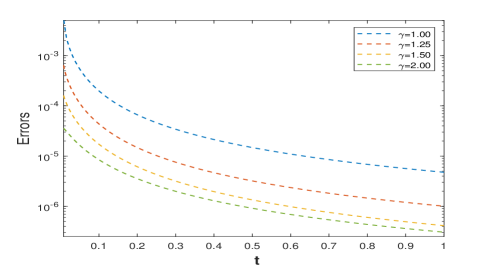
Figure 1: Pointwise error $\|U_{h}^{n}-u(t_{n})\|$ as a function of $t_{n}$ for $N=128$, $\alpha=0.6$, and different values of $\gamma\geq 1$.

The time convergence rate $r_{t}$ is subsequently calculated from the relation $r_{t}\approx{\rm log}_{2}\big{(}\epsilon_{N}/\epsilon_{2N}\big{)}.$ It is not difficult to show that the data of the problem satisfy the conditions of the stability and convergence Theorems 7 and 15 for $1/2<\alpha<1$. Furthermore, because of the inequality

$$\Big{|}\frac{d^{j}}{dt^{j}}E_{\alpha,1}(-\lambda_{m}^{2}t^{\alpha})\Big{|}\leq C(\lambda_{m}^{2}t^{\alpha})^{-\mu}t^{-j},\quad\mbox{for }j\in\{1,2,3,\cdots\}\mbox{ and }|\mu|\leq 1,$$

the first regularity estimate in (4) holds true for $0<\alpha<1$, and the second one is valid for $\sigma=\alpha^{-}/4$. This result is supported by the regularity analysis presented in (McLean (2010) and McLean et al. (2020)), because $u_{0}\in\dot{H}^{2.5^{-}}(\Omega)\cap H^{1}_{0}(\Omega)$ and the source term $f$ satisfies the inequality $t^{j}\|f^{(j)}(t)\|_{1}\leq Ct^{\frac{3\alpha}{4}-1}$ for $t>0,$ with $j=0,1,2,3$. Therefore, for $1/2<\alpha<1$, by Theorem 15,

$$r_{t}=\begin{cases}\sigma+\alpha/2\approx 3/(4\alpha^{-})&\quad{\rm when}~{}~{}\gamma=1,\\ 2&\quad{\rm when}~{}~{}\gamma>2/(\sigma+\alpha/2)\approx 8/(3\alpha^{-})\,.\end{cases}$$

Table 1 presents $\epsilon_{N}$ and $r_{t}$, for $\alpha=0.7$ and for different choices of $\gamma\geq 1$. As expected, $\epsilon_{N}$ and $r_{t}$ improve with $\gamma$. The empirical convergence rate is found to be better than expected with $r_{t}\approx(\sigma+\alpha)\gamma$ for $1\leq\gamma\leq 2/(\sigma+\alpha)\approx 2.3.$ Further, Table 2 reports similar convergence rates for $\alpha=0.5$ (top part) and $\alpha=0.4$ (bottom part), that is, when $\alpha$ is outside the range covered by the theory.

$N$	$\gamma=1$		$\gamma=1.6$		$\gamma=2.3$
16	2.039e-02		3.787e-03		8.847e-04
32	1.022e-02	0.9964	1.417e-03	1.4187	2.234e-04	1.9856
64	4.976e-03	0.1038	5.446e-04	1.3792	5.638e-05	1.9863
128	2.578e-03	0.9486	2.065e-04	1.3990	1.421e-05	1.9880
256	1.417e-03	0.8640	7.816e-05	1.4018	3.588e-06	1.9863

Table 1: Errors $\epsilon_{N}$ and convergence rates $r_{t}\approx(\sigma+\alpha)\gamma$ for $\alpha=0.7$, and different choices of $1\leq\gamma\leq 2/(\sigma+\alpha)$.

$\alpha=0.5$
$N$	$\gamma=1$	$\gamma=1.6$	$\gamma=2.4$	$\gamma=3.2$
32	2.5e-02    0.458	6.7e-03    1.082	1.0e-03    1.568	2.6e-04    1.953
64	1.7e-02    0.551	3.0e-03    1.139	3.7e-04    1.489	6.8e-05    1.954
128	1.1e-02    0.634	1.5e-03    1.065	1.3e-04    1.499	1.7e-05    1.962
256	6.7e-03    0.693	7.3e-04    0.999	4.6e-05    1.502	4.5e-06    1.966
$\alpha=0.4$
$N$	$\gamma=1$	$\gamma=2$	$\gamma=3$	$\gamma=4$
32	2.9e-02    0.276	6.4e-03    1.029	9.7e-04    1.604	2.8e-04    1.913
64	2.3e-02    0.331	2.9e-03    1.126	3.4e-04    1.496	7.4e-05    1.921
128	1.8e-02    0.388	1.4e-03    1.089	1.2e-04    1.497	1.9e-05    1.936
256	1.3e-02    0.444	6.8e-04    1.016	4.3e-05    1.502	5.0e-06    1.945

Table 2: Errors $\epsilon_{N}$ and convergence rates $r_{t}$ for different choices of $1\leq\gamma\leq 2/(\sigma+\alpha)$. It is observed that $r_{t}\approx{(\sigma+\alpha)\gamma}$.

Example 2. The second example considers a solution with lower regularity. We choose $u_{0}(x)=x$ on $[0,1/2]$ and $1-x$ on $[1/2,1]$. Thus, $u_{0}\in H^{1.5^{-}}(\Omega)$. The source term $f$ is chosen so that

$$u(x,t)=4\sum_{m=0}^{\infty}(-1)^{m}\lambda_{m}^{-2}\sin(\lambda_{m}x)E_{\alpha,1}(-\lambda_{m}^{2}t^{\alpha}),\quad\lambda_{m}:=(2m+1)\pi.$$ (20)

Following similar arguments as of the previous example, we deduce that the first regularity estimate in (4) holds for $0<\alpha<1$, while the second one is valid only for $\sigma=-\alpha^{+}/4<0.$ Thus, the required regularity assumptions of Theorems 15 are not satisfied. To avoid dealing with negative values of $\sigma,$ we focus on the weighted error $t_{n}^{\alpha/4}\|U_{h}^{n}-u(t_{n})\|$ (so $\sigma^{*}=\sigma+\alpha/4\approx 0$) and the corresponding convergence rates. We denote $\epsilon^{*}_{N}=\max_{1\leq n\leq N}\,t_{n}^{\alpha/4}\|U^{n}_{h}-u(t_{n})\|,$ and $r_{t}^{*}$ the associated rate of convergence.

Table 3 reports $\epsilon^{*}_{N}$ and $r_{t}^{*}$ for $\alpha=0.4$, 0.6 and 0.8, and different $\gamma$ in the range $[1,2/\alpha]$. As in the previous example, the empirical results confirmed $r_{t}^{*}\approx\min\{\gamma(\sigma^{*}+\alpha),2\}\approx\min\{\gamma\alpha,2\}$-rates of convergence. Therefore, at time level $t_{n},$ we may conclude that the error $\|U_{h}^{n}-u(t_{n})\|\leq Ct_{n}^{-\alpha/4}\tau^{\min\{\gamma\alpha,2\}}$. When $\gamma=1$ (uniform time meshes), such as estimate is expected in the limiting case $\alpha\to 1$ (the fractional Fokker-Planck (1) reduces to the classical Fokker-Planck model).

$\alpha=0.4$
$N$	$\gamma=1$	$\gamma=2$	$\gamma=3$	$\gamma=5$
32	3.4e-02    0.363	6.75e-03    9.716	1.7e-03    1.159	1.8e-04    1.928
64	2.5e-02    0.409	3.72e-03    8.581	7.3e-04    1.186	4.7e-05    1.937
128	1.8e-02    0.452	2.18e-03    7.730	3.2e-04    1.198	1.2e-05    1.949
256	1.3e-02    0.482	1.27e-03    7.782	1.4e-04    1.199	3.1e-06    1.958
$\alpha=0.6$
$N$	$\gamma=1$	$\gamma=2$	$\gamma=2.6$	$\gamma=3.3$
32	1.9e-02    0.748	2.1e-03    1.155	6.1e-04    1.557	1.7e-04    1.965
64	1.1e-02    0.741	9.3e-04    1.196	2.1e-04    1.559	4.3e-05    1.982
128	7.1e-03    0.654	4.1e-04    1.199	7.2e-05    1.559	1.1e-05    1.986
256	4.7e-03    0.579	1.8e-04    1.199	2.4e-05    1.561	2.8e-06    1.987
$\alpha=0.8$
$N$	$\gamma=1$	$\gamma=1.5$	$\gamma=2$	$\gamma=2.5$
32	0.0e-03    0.824	2.4e-03    1.181	5.9e-04    1.599	1.7e-04    2.031
64	5.4e-03    0.733	1.0e-03    1.200	1.9e-04    1.599	4.2e-05    2.000
128	3.1e-03    0.780	4.5e-04    1.199	6.5e-05    1.599	1.0e-05    1.997
256	1.8e-03    0.801	2.0e-04    1.199	2.1e-05    1.601	2.7e-06    1.969

Table 3: Weighted errors $\epsilon^{*}_{N}$ and associated convergence rates for Example 2, with different choices of $\alpha$ and $\gamma\geq 1$. The time convergence rate is $\approx{(\sigma^{*}+\alpha)\gamma}$ for $1\leq\gamma\leq 2/(\sigma^{*}+\alpha)$, where in this example $\sigma^{*}=\sigma+\alpha/4\approx 0$.

References

• [1] C. N. Angstmann et al. (2015), Generalised continuous time random walks, master equations and fractional Fokker–Planck equations, SIAM J. Appl. Math., 75, 1445–1468.
• [2] H. Brunner, A. Pedas, and Vainikko (1999), The piecewise polynomial collocation method for weakly singular Volterra integral equations. Math. Comp., 68, 1079–1095.
• [3] G. A. Chandler and I. G. Graham (1988), Product integration-collocation methods for noncompact integral operator equations, Math. Comp., 50, 125–138.
• [4] C. Huang, K.-N. Le, and M. Stynes (2020). A new analysis of a numerical method for the time-fractional Fokker–Planck equation with general forcing, IMA J. Numer. Anal., 40, 1217–1240.
• [5] W. Deng (2007), Numerical algorithm for the time fractional Fokker-Planck equation, J. Comput. Phys., 227, 1510–1522.
• [6] J. Dixon and S. McKee (1986), Weakly singular Gronwall inequalities, ZAMM Z. Angew. Math. Mech., 66, 535–544.
• [7] M. H. Duong and B. Jin (2020), Wasserstein Gradient Flow Formulation of the time fractional Fokker-Planck equation, arXiv: 1908.09055v2.
• [8] B. Jin, B. Li, and Z. Zhou (2018) Numerical analysis of nonlinear subdiffusion equations. SIAM J. Numer. Anal., 56, 1–23.
• [9] Y. Jiang and X. Xu (2019), A monotone finite volume method for time fractional Fokker-Planck equations, Sci. China Math., 62, 783–794.
• [10] S. Karaa and A. Pani (2020), Mixed FEM for time-fractional diffusion problems with time-dependent coefficients, J. Sci. Comput., 83.
• [11] N. Kopteva (2019), Error analysis of the $L1$ method on graded and uniform meshes for a fractional-derivative problem in two and three dimensions, Math. Comp., 88, 2135–2155.
• [12] K.-N. Le, W. McLean, and M. Stynes (2019), Existence, uniqueness and regularity of the solution of the time-fractional Fokker–Planck equation with general forcing, Comm. Pure. Appl. Anal., 18, 2765–2787.
• [13] K. N. Le, W. McLean, and K. Mustapha (2016), Numerical solution of the time-fractional Fokker-Planck equation with general forcing, SIAM J. Numer. Anal., 54, 1763–178.
• [14] K. N. Le, W. McLean, and K. Mustapha (2018), A semidiscrete finite element approximation of a time-fractional Fokker–Planck equation with nonsmooth initial data, SIAM J. Sci. Comput., 40, A3831–3852.
• [15] H.-l. Liao, W. McLean, and J. Zhang (2019), A discrete Gronwall inequality with applications to numerical schemes for subdiffusion problems, SIAM J. Numer. Anal., 57, 218–237.
• [16] W. McLean (2010), Regularity of solutions to a time-fractional diffusion equation, ANZIAM J., 52, 123–138.
• [17] W. McLean and Mustapha (2007), A second-order accurate numerical method for a fractional wave equation, Numer. Math., 105, 481–510.
• [18] W. McLean et al. (2019), Well-posedness of time-fractional advection-diffusion-reaction equations, Fract. Calc. Appl. Anal., 22, 918–944.
• [19] W. McLean et al. (2020), Regularity theory for time-fractional advection–diffusion–reaction equations, Comp. Math. Appl., 79, 947–961.
• [20] W. McLean and K. Mustapha (2021), Uniform stability for a spatially-discrete, subdiffusive Fokker–Planck equation, Numer. Algo., to appear.
• [21] K. Mustapha (2015), Time-stepping discontinuous Galerkin methods for fractional diffusion problems. Numer. Math., 130, 497–516.
• [22] K. Mustapha (2020), An L1 approximation for a fractional reaction-diffusion equation, a second-order error analysis over time-graded meshes, SIAM J. Numer. Anal., 58, 1319–1338.
• [23] M. Stynes (2021), A survey of the L1 scheme in the discretisation of time-fractional problems, www.researchgate.net/profile/Martin-Stynes/publication/348409672
• [24] M. Stynes, E. O’Riordan, and J. L. Gracia (2017), Error analysis of a finite difference method on graded meshes for a time-fractional diffusion equation, SIAM J. Numer. Anal., 55, 1057–1079.
• [25] A. Saadatmandi, M. Dehghan, and M.-R. Azizi (2012), The sinc–Legendre collocation method for a class of fractional convection-diffusion equations with variable coefficients, Commun. Nonlinear Sci. Numer. Simul., 17, 4125–4136.
• [26] F. Wang, Y. Zhao, C. Chen, Y. Wei, and Y. Tang (2019), A novel high-order approximate scheme for two-dimensional time-fractional diffusion equations with variable coefficient, Computers & Mathematics with Applications, 78, 1288–1301.
• [27] Y. Yan, M. Khan, and N. J. Ford (2018), An analysis of the modified $L1$ scheme for time-fractional partial differential equations with nonsmooth data, SIAM J. Numer. Anal., 56, 210–227.
• [28] Y. Yang, Y. Huang, and Y. Zhou (2018), Numerical solutions for solving time fractional Fokker-Planck equations based on spectral collocation methods, J. Comput. Math., 339, 389–404.
• [29] H. Ye, J. Gao, and Y. Ding (2007), A generalized Gronwall inequality and its application to a fractional differential equation, J. Math. Anal. Appl., 328, 1075–1081.