An Approach to Causal Inference over Stochastic Networks

Abstract

Claiming causal inferences in network settings necessitates careful consideration of the often complex dependency between outcomes for actors. Of particular importance are treatment spillover or outcome interference effects. We consider causal inference when the actors are connected via an underlying network structure. Our key contribution is a model for causality when the underlying network is endogenous and co-evolves with the actor covariates stochastically over time. We develop a joint model for the relational and covariate generating process that avoids restrictive separability and deterministic network assumptions as these rarely hold realistic social network settings. Our framework utilizes the highly general class of Exponential-family Random Network models (ERNM) of which Markov Random Fields (MRF) and Exponential-family Random Graph models (ERGM) are special cases. We present potential outcome based inference within a Bayesian framework, and propose a modification to the exchange algorithm to allow for sampling from ERNM posteriors. We present results of a simulation study demonstrating the validity of the approach. Finally, we demonstrate the value of the framework in a case-study of smoking over time in the context of adolescent friendship networks.

1 Introduction

Causal inference is difficult, especially in systems with partially known and likely complex structure. There is an extensive literature on causal inference methods for so called “network settings” from a variety of perspectives (Hudgens and Halloran, 2008; Shalizi and Thomas, 2011; Ogburn and VanderWeele, 2014; van der Laan, 2014; Sofrygin and van der Laan, 2017; DeAmour, 2016; Aronow and Samii, 2017; Shpitser et al., 2021; Tchetgen Tchetgen et al., 2020; Ogburn et al., 2020).

There are recent empirical studies claiming strong causal results in network settings that have been controversial. For example, claims about the spread of characteristics through social settins, so called social contagion (Christakis and Fowler, 2007, 2008, 2010) with corresponding methodological criticism from others (e.g. Ogburn et al., 2020). Such results are controversial due not only to their surprising and perhaps provocative substantive nature, for example, statements such as “obesity is socially contagious”, but also due to the strong assumptions required to justify the methodology.

Much of the problem stems from the unknown underlying social processes. For example, as explicitly noted in Shalizi and Thomas (2011), contagion is often confounded with homophily. They consider Directed Acyclic Graphs (DAGs) (Pearl, 1995; Spirtes et al., 2000) and demonstrate that contagion can be confounded when latent homophily is present.

In this paper we consider social structures represented by networks with stochastic links and covariates that stochastically co-evolve over time. We present a generalized chain graph approximation to a credible social process DAG, which allows for a dependence structure that we believe to be compatible with such problems. We seek causal inference, that is the effect on outcomes of a hypothetical intervention. We then frame causal inference in terms of network equilibrium potential outcomes, that is, potential outcomes derived from the chain graph structure, and use an augmented variable Markov Chain Monte Carlo (MCMC) algorithm to sample from their posterior distributions. The key contribution of our approach is to allow for uncertainty in the network structure and for codependence of edges and nodal covariates in the underlying social process over time.

Chain graphs have been posited as a possible representation of the causal structure of networks evolving over time that reach equilibrium (Tchetgen Tchetgen et al., 2020; Shpitser et al., 2021). By considering a DAG of a network generating process over time, Ogburn et al. (2020) and Lauritzen and Richardson (2002) suggest that estimating causal effects in this setting is not viable unless fine grained temporal data is available and the causal structure is simple.

We consider the situation where we observe a single network, considered a realization of a random social process over both nodes and edges. Causal inference in this setting cannot be reduced to an independent and identically distributed (IID) problem in the same fashion as Sofrygin and van der Laan (2017). The chain graph approximation employed in Tchetgen Tchetgen et al. (2020) and Ogburn et al. (2020) cannot be used as it does not allow for stochastic connections. There have been efforts to allow for network uncertainty (Toulis and Kao, 2013; Kao, 2017). However these methods require unconfoundedness of the edges and the random nodal covariates, given enough fixed information about the nodes. In not making such an assumption we require a joint probability model for the random edges and nodal covariates in the graph.

We note that the literature of network causal inference is at present sharply disconnected from the literature concerning generative models for social networks. As most approaches have considered the networks as fixed, there has been little interest in placing a probability distribution over the space of possible networks. Typically generative models for social networks for example the commonly used Exponential-family Random Graph Models (ERGM) (Frank and Strauss, 1986) consider the edges as the random variables to be modelled and nodal covariates as fixed. There has been much sophisticated work on understanding such models (Handcock, 2003; Robins et al., 2007; Schweinberger and Handcock, 2015), and well developed MCMC based fitting procedures (Snijders, 2002; Handcock, 2002) with associated complex software (Hunter et al., 2008). However due to the assumed fixed nature of the nodal covariates, these are of limited use for causal inference on nodal outcomes. Markov random field (MRF) models treat the nodal covariates as stochastic but the connections between nodes fixed. Encompassing both model classes are the novel Exponential-family Random Network Model (ERNM) (Fellows and Handcock, 2012). ERNM are a class of exponential family models that encompasses ERGMs and MRF as special cases. ERNM allows for the edges and nodal covariates to be stochastic, thus the nodal covariates and the edges can be co-dependent. The focus of this paper is causal inference based on the plausible representation of complex social structure via ERNM.

We utilize a Bayesian framework for the causal quantities and the network model. This allows for the incorporation of prior information, as well the automatic accounting of uncertainty in a theoretically consistent manner. The Bayesian approach does not require appeals to asymptotic arguments for its validity. Indeed, asymptotics for causal quantities in our setting are conceptually difficult as there is no single asymptotic framework that is compelling. In particular, the number of nodes, $N$, is a fundamental characteristic of the social process and not a sampling design characteristic, as it is in most of Statistics. For example, the interactions of a class with 5 students will be quite different from a class of size 75. Hence asymptotic approximations must identify credible invariant parametrisations (Krivitsky et al., 2011). Different values of $N$ change the fundamental structure of the social network, as dependent edge behaviour is strongly related to the number of nodes in a network. We develop a modification to the exchange algorithm (Murray et al., 2006) to allow for sampling from ERNM posteriors, which we use to infer the posterior distributions of potential outcomes and, hence, estimate causal estimands of interest.

This paper is structured as follows. Section 2 introduces our general network setting and our notation. Section 4 considers the DAG of a network process over time allowing for network uncertainty with a chain graph approximation. Section 3 defines causal quantities of interest in terms of equilibrium potential outcomes. Section 6 briefly describes a simulation study, the details of which are contained in the supplement. Section 7 considers a case-study of a network from the National Longitudinal Study of Adolescent Health (Harris et al., 2007) and gives estimates of unknown causal quantities. Section 8 provides general discussion of the method, and its ability to generate credible causal inference.

2 Notation and Setting

We consider a known fixed set of $N$ nodes. Each node has a random nodal outcome $Y_{i}$, thus the whole network outcome is $Y=(Y_{1},\ldots Y_{N})$. Realizations of the random nodal covariates $Y_{i}$ and $Y$ are denoted with lower case $y_{i}$ and $y$. For this paper we only consider binary outcomes (although the ideas are easily extended to non-binary outcomes). Each node is also permitted to have further multivariate nodal covariates similarly denoted $X=(X_{1},\ldots X_{N})$ with $X_{i}\in\mathbb{R}^{p}$ for some p.

We denote the random edges between nodes as the random variable $A=\{A_{i,j}\}_{i=1,j=1}^{N}$, with realizations $a$. $A$ can be considered a random adjacency matrix. We also restrict $A_{i,j}$ to be binary with $1$ indicating a connection and $0$ representing the absence of a connection. For this paper, we make the restriction that our networks are undirected i.e. $A_{i,j}=A_{j,i}\quad\forall i,j$.

A network realization is defined to be a set $\{y,a,x\}$. When considering the dynamic network of the process over time we indicate the outcomes at time $t$ with superscript, for example, the outcome random variable for node $i$ at time $t$ is $Y_{i}^{t}$ and the whole network random variable at time t is $\{Y^{t},A^{t},X^{t}\}$. If the temporal dynamics result in an equilibrium distribution, we denote it by $\underset{t\rightarrow\infty}{\lim}\left(Y^{t},A^{t},X^{t}\right)=\left(Y,A,X\right)$.

As the node set is fixed, the nodal covariates $X$ are often in practice fixed throughout the evolution of the social process. Going forward we omit $X$ from our notation, that is for clarity, we consider our networks as realizations of $\left(Y,A\right)|X=x_{observed}$ but write $\left(Y,A\right)$.

We represent the treatment of nodes via the treatment vector $Z=(z_{1},\ldots z_{N})$ with realizations $z$. For the purposes of this paper we consider the treatment to be applied prior to the evolution of the network process though perhaps conditional on the fixed nodal covariates. We leave allowing for time varying treatments assignments and outcome evolution to future research, though we believe it to be compatible with our approach.

In the following section we will introduce a DAG to represent the dependence structure of the social network. We emphasize that the nodes in the DAGs represent random variables in the stochastic social process underlying the above described social network setting (rather than actors in the social network). That is, nodes in the DAG represent random variables in the social process generating the network, they may either be treatments, random nodal covariates, or random edges.

3 Network Potential Outcomes and Causal Estimands of Interest

Hudgens and Halloran (2008), Toulis and Kao (2013) and Aronow and Samii (2017) all considered potential outcome-based frameworks of assumptions and definitions as a basis for causal inference for nodal covariates. We consider network potential outcomes as realizations of an equilibrium distribution of a social process that evolved over time.

Our causal estimands should be interpreted as the effect of an intervention on the equilibrium distribution, this is implicit in Toulis and Kao (2013) and Aronow and Samii (2017). Estimands in Tchetgen Tchetgen et al. (2020) and Ogburn et al. (2020) are based interventions on nodal statuses prior to the evolution of the social process, and estimate network effects, rather than nodal effects. We note that these whole network direct or spillover treatment outcomes for pre social processes interventions, the ERNM (Fellows and Handcock, 2012) presented in Section 5.2 is still fully compatible with such regimes, and indeed a generalization of the MRF models used in Tchetgen Tchetgen et al. (2020) and Ogburn et al. (2020).

We set $Y_{i}(Z,A,Y_{-i})$ to be the equilibrium potential outcome of node $i$, given the treatment vector of all nodes $Z$, the network $A$, and the outcomes of all the other nodes $Y_{-i}$. In this definition, each potential outcome $i$ depends fully on the entire rest of the edges and nodal potential outcomes in the network. However as our estimands of interest relate to one-step neighbourhoods of nodes, we make the following assumption.

The one-step neighbourhood, assumptions also allows us to dramatically reduce the required number of simulations to estimate missing potential outcomes in section 5.

Assumption 1

One Step Neighbourhoods

$$\forall i\qquad Y_{i}(Z,A,Y_{-i})=Y_{i}(Z_{i},Z_{\mathscr{N}_{i}(A)},\mathscr{N}_{i}(A),Y_{\mathscr{N}_{i}(A)})$$ (1)

where $\mathscr{N}_{i}(A)$ is the neighbourhood of node $i$ in the network $A$. That is, the individual outcomes only depend on treatments, edges and outcomes in their own one-step neighbourhood.

We next state the causal estimands that we will pursue in their full generality. In section 5 we will consider models, and simplifying assumptions that allow for inference in practice.

Definition 1

Primary Effects

$$\xi_{i} =\frac{1}{|(Z^{-i},A,Y^{-i})|}\sum_{(z^{-i},a,y^{-i})\in(Z^{-i},A,Y^{-i})}Y_{i}(z_{i}=1,z,a,y)-Y_{i}(z_{i}=0,z,a,y)$$ (2)

$$\xi^{ave} =\frac{1}{N}\sum_{i=1}^{N}\xi_{i}$$ (3)

where $(Z^{-i},A,Y)$ are all possible combinations of edges, outcomes and treatments excluding the outcome and treatment of node i.

Definition 2

$k$-peer Treatment Effect

$$\delta^{k}_{i} =\frac{1}{|(Z,A)_{\mathscr{N}_{i}}|}\sum_{(z,a,y)\in(Z,A)^{k}_{\mathscr{N}_{i}}}Y_{i}(z_{i}=0,z,a,y)-Y_{i}(z_{i}=0,(z,a)\in(Z,A)^{0}_{\mathscr{N}_{i}},y)$$ (4)

$$\delta_{k} =\frac{1}{N}\sum_{i=1}^{N}\delta^{k}_{i}$$ (5)

where $(Z,A)^{k}_{\mathscr{N}_{i}}$ is the set of combinations of node-i-local edge realizations and treatment assignments such that node $i$ is exposed to $k$ other treated nodes.

Definition 3

$k$-peer Outcome Effect For Binary Outcomes

$$\delta^{k}_{i} =\frac{1}{|(A,Y)_{\mathscr{N}_{i}}|}\sum_{(z,a,y)\in(A,Y)^{k}_{\mathscr{N}_{i}}}Y_{i}(z_{i}=0,z,a,y)-Y_{i}(z_{i}=0,z,(a,y)\in(A,Y)^{0}_{\mathscr{N}_{i}})$$ (6)

$$\delta_{k} =\frac{1}{N}\sum_{i=1}^{N}\delta^{k}_{i}$$ (7)

where $(A,Y)^{k}_{\mathscr{N}_{i}}$ is the set of combinations of node-i-local edge and outcome realizations such that node $i$ is exposed to $k$ other nodes with outcome $1$.

We note that the $k$-peer outcome effect could be considered as a special case of a $k$-peer treatment effect where the treatment results in outcome $1$, almost surely. However we find it convenient to express the estimand separately as it is often of substantive interest in networks where some other treatment is administered, but the $k$-peer outcome effect is important.

4 Causal Framework

DAGs provide a means for precisely specifying the structure of relationships between random variables (see Pearl (2009) for an introduction). Pearl (1995) developed strict criteria for identification of causal effects. Formal equivalence with the potential outcome framework was shown in Richardson and Robins (2013)

Nodes in the DAG represent random variables, with edges drawn between nodes being strictly uni-directional, and cycles of edges prohibited, so that so called “feedback” loops are not permitted. The interpretation of a directed line from node $i$ to node $j$ is that $i$ causally effects $j$. For a node indexing set $V$, denote the corresponding random variables $\{x_{v}\}_{v\in V}$. This graphical structure encodes the following factorization of their joint probability distribution $p(x)=\prod_{v\in V}p(x_{v}|x_{pa(v)})$, where $pa(v)$ are the parents of $v,$ that is the nodes in the DAG with edges into $v$.

The causal effect of $X$ on $Y$ is represented by $p(y|do(X=x)),$ the distribution of the random variable $Y$ when $X$ has been externally set to $x$. Pearl (2009) provides transformations for expressing this new distribution $p(y|do(X=x))$ in terms distribution on observed random variables e.g. $p(y|x)$ or $p(y|x,z)$ for $z$ some other variable in the system.

Chain graphs permit undirected as well as directed edges, which allow for different Markov properties from DAGs. In fact chain graphs can represent dependence structures that are not possible under a DAG. We include some discussion in the supplement however we omit subtleties of their Markov properties discussed in Frydenberg (1990) and utilized for causal analysis in Lauritzen and Richardson (2002). In their full generality, chain graphs can express complex dependence structures. However, in our case, our example chain graph only has one chain component which results in none of the outcomes being rendered conditionally independent, thus we do not require an in-depth review for the purposes of this paper. Practically, one possible interpretation of the undirected edges in a chain graph is that the two variables interact in a causal feedback sense over time.

DAGs representing the causal structure of outcomes of nodes in networks under both interference and contagion are given a clear and detailed treatment in Ogburn and VanderWeele (2014). We generalize the related conjecture in Ogburn et al. (2020) for a chain graph approximation of causal structure of a social network, which slowly evolves over time. This is based on an interpretation of causality with feedback relationships over time which chain graphs can be used to explain (Lauritzen and Richardson, 2002). Our generalization is to consider a social network where the connections are not fixed and are motivated by the empirical observation that social connections are often strongly dependent on other nodes’ connections as well as other nodes’ covariates, treatments and outcomes.

As an illustration for our chain graph approximation, Figure 1 represents the structure of a network evolving over time for a three node network similar to that of Ogburn et al. (2020) and Tchetgen Tchetgen et al. (2020). Note the analogous connections between node 3 and 1 are omitted for clarity. Block arrows denote multiple arrows into the variables described therein. The full DAG with all arrows becomes quickly unwieldy. In the notation of Section 2, the nodal treatments are $\{Z_{1},Z_{2},Z_{3}\}$, nodal outcome variables $\{Y_{1},Y_{2},Y_{3}\}$, and we denote the undirected edges between nodes $i$ and $j$ as $A_{i,j}$. Directed network edges as well as fixed nodal covariates can also be built-in but are omitted here for clarity. Superscripts denote the status of a variable at that time step e.g. $Y_{2}^{t}$ is the outcome for node $2$ at time $t$.

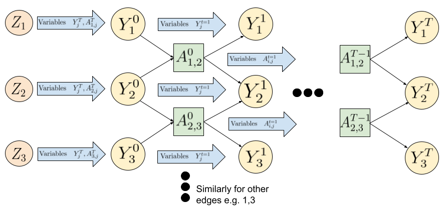
Figure 1: Full DAG of temporal network formation feedback process, in the three node network case. Treatment variables $Z_{j}$ are permitted to causally effect all of the other variables. Outcomes $Y_{i}^{t}$ and $Y_{j}^{t}$ are permitted to causally effect edges $A^{t}_{i,j}$, as well as outcomes $Y_{i}^{t+1}$ and $Y_{j}^{t+1}$. Edges $A_{i,j}^{t}$ are permitted to causally effect edges $A_{k,l}^{t+1}$ with no restrictions on $k$ and $l$. In practice the functional form of models will usually restrict the causal impact of node $i$’s outcome and treatment to only the set of neighbouring nodes $\{j\}$, that is, where there is an edge present between node $i$ and $j$.

Under this DAG, each of the treatment variables $Z_{j}$ are permitted to causally effect all of the other outcome variables, as well as edges involving $j$. Outcomes $Y_{i}^{t}$ and $Y_{j}^{t}$ are permitted to causally effect edges $A^{t}_{i,j}$, as well as outcomes $Y_{i}^{t+1}$ and $Y_{j}^{t+1}$. Edges $A_{i,j}^{t}$ are permitted to causally effect edges $A_{k,l}^{t+1}$ with no restrictions on $k$ and $l$.

We note that there are key edges that are not present in this DAG. Edges and outcomes, from time step $t$ can only influence edges and outcomes at time step $t+1$, not others. We argue that this is plausible under slow evolution of a network process over time. In general, it is exceedingly rare that enough data are available to identify all the relationships posited in Figure 1.

The DAG for our system is highly complex, and we usually observe little incremental time data on the social process. Thus operations as introduced in Pearl (1995) to reduce $p(y|do(X=x))$ to expressions involving only distributions, from which we have realizations, e.g., $p(y|x)$, are not possible. That is the true causal effect is unidentifiable. We pursue “approximate causal inference” through approximating the DAG for our social process over time with a chain graph.

As noted in Lauritzen and Richardson (2002), the equilibrium distribution of a so called infinite DAG can be represented as a chain graph. Similarly to Ogburn et al. (2020), but modelling edges as random, the DAG in Figure 1 can be approximated by the chain graph shown in Figure 2. The chain component (undirected component) of this chain graph is close to being complete since we allow every nodal outcome to influence every other nodal outcome, however we only allow outcomes $Y_{i}$ and $Y_{j}$ to influence edge $A_{i,j}$. In the full DAG, backdoor paths through previous time steps result in this not being the case.

This suggests that the complex structure of such a DAG can be approximated with the chain graph factorization:

$$p(Y,A,Z)=\left(\prod_{i=1}^{n}p(z_{i})\right)p(Y,A|Z)$$ (8)

As an approximation to the true temporal DAG a chain graph model of causality serves to render the causal effects tractable in practice. See Ogburn et al. (2020) and Lauritzen and Richardson (2002) for a fuller explanation.

As an illustration of the generality of this chain graph’s dependence structure we define a conditional independence property, that we refer to as local conditional independence as follows:

$$Y_{i}^{T}\perp\!\!\!\perp Y_{j}^{T},Z_{j}~{}~{}\Bigg{|}~{}~{}A_{i,j}^{T}=0,~{}~{}Z_{i},~{}~{}\{Y_{l}^{T}:A_{i,l}^{T}=1\}$$ (9)

That is, nodal outcomes are conditionally independent given all neighbours, and that they are not connected. Equation (9) does not hold a priori due to the dependence induced by the random edge $A_{i,j}$ unlike in the fixed network case where it does. That is, the chain graph retains dependencies between outcomes of non-connected nodes, even when conditioning on neighbours. In fact, due to the close-to-complete nature of the chain component, there are few conditional independence assumptions that can be concretely made. Indeed the complexity of such systems is the reason why social network modelling has proven to be difficult.

Figure 2: Chain graph approximation of a three node temporal social network process with treatment

Conditional independence properties have been considered for ERGMs (Snijders et al., 2006). Common properties induced by model choice in ERGMs are the so-called Markov property (Frank and Strauss, 1986) and the so called social circuit property that requires the Markov property in addition to a cycle condition (Snijders et al., 2006). Both of these commonly imposed assumptions severely limit possible dependence structures. In practice the social network modelling community has found the social circuit assumption to yield well fitting models in a wide variety of situations (Goldenberg et al., 2010).

We do not comment on the validity of the approximation of the DAG by the chain graph. Ogburn et al. (2020) gave simulations supporting their version of this approximation. We will only consider recovering causal estimands based on the assumption that the chain graph approximation holds.

The remainder of this paper concerns modelling $P(Y,A|Z)$ in order to estimate causal quantities. We specify our causal estimands using equilibrium distribution potential outcomes. Implicitly the assumption we make in the DAG formulation, under some intervention on the equilibrium denoted with a superscript $*$.

$$P_{equil}(Y_{i}=y|(A,Z,Y_{i}^{c})=(A,Z,Y_{i}^{c})^{\ast})=P_{equil}(Y_{i}=y|\text{do}((A,Z,Y_{i}^{c})=(A,Z,Y_{i}^{c})^{\ast})$$ (10)

We note that intervening on an equilibrium distribution is not possible in practice. However in order to claim the estimation of causal quantities, which are intertwined with social processes, we believe it to be necessary as well as implicit in current potential outcome based approaches (Aronow and Samii, 2017; Toulis and Kao, 2013). We interpret our causal estimands as an average, of the possible treatments, and social processes that led to a given treatment in equilibrium.

The lack of conditional independence assumptions that we are able to make in Section 5, is the direct consequence of the nearly complete chain graph model specified in this section.

5 Estimation and Identifying Assumptions

Section 3 introduced network potential outcomes and our estimands of interest. Section 4 justified that they have a casual interpretation. In this section we will introduce models that can be practically used to infer the missing potential outcomes, to produce concrete estimates of causal effects.

Our strategy is to pursue model-based Bayesian imputation of potential outcomes (Imbens and Rubin, 2015).

5.1 Structural Assumptions

We next state possible assumptions restricting the dependence structure of the process that will enable us to feasibly impute missing potential outcomes from network simulations. In our assumptions we explicitly include fixed nodal covariates $X$.

Assumption 2

Unconfounded Treatment Assignment Assumption Under Network Assignment

$$P(Z|X,A,\mathbb{Y})=P(Z|X,A,\mathbb{Y}^{\prime})\quad\forall Z,X,A,\mathbb{Y}\quad and\quad\mathbb{Y}^{\prime}$$

where $A$ is a network, X is a set of nodal covariates on the nodes, and $\mathbb{Y}$ are the potential outcomes.

To account for uncertainty in the network it is possible to make the assumption, as in Kao (2017), that the causal link between the network and outcomes can be broken by the inclusion of nodal covariates. Specifically:

Assumption 3

Unconfounded Network Assumption under Network Interference

$$P(A|X,\mathbb{Y})=P(A|X,\mathbb{Y}^{\prime})\quad\forall A,X,\mathbb{Y}\quad and\quad\mathbb{Y}^{\prime}$$

We note that Assumption 2 also follows as a consequence of the chain graph approximation, as in the three node example in Figure 2 (See Lauritzen and Richardson, 2002, for discussion on this).

Assumption 3 essentially assumes away the main problem of network causal inference, that the network structure and the potential outcomes are related. The idea is that after including enough nodal covariates, the association between the network and the nodal potential outcomes breaks down. Note that this assumption trivially holds if the network is considered fixed.

Denoting the missing potential outcomes as $\mathbb{Y}_{miss}$ and the observed as $\mathbb{Y}_{obs}$. Using Assumptions 1 and 2, Kao (2017) show that :

$$P(\mathbb{Y}_{miss}|X,Z,A,\mathbb{Y}_{obs})=P(\mathbb{Y}_{miss}|X,\mathbb{Y}_{obs})$$ (11)

Kao (2017) propose choosing covariates $X$ to include so that Assumption 3 is met, and suggest that the addition of covariates derived from modelling the network $A$ may be included to achieve this.

We require only Assumptions 1 and 2, and modelling the potential outcomes jointly with the network. We argue that this is more realistic in most situations, and forces the researches into more realistic modelling choices to arrive at causal inference for nodal outcomes.

The relaxation of Assumption 3 breaks down the proof of Equation (11), with the analogous result under the relaxed assumption being:

$$P(\mathbb{Y}_{miss}|X,Z,A,\mathbb{Y}_{obs})=P(\mathbb{Y}_{miss}|X,A,Y_{obs})$$ (12)

The retention of the network $A$ in the conditioning variables, requires that we model its posterior distribution in the imputation of the missing potential outcomes.

5.2 Modelling

To facilitate modelling when the network is not fixed, we use the ERNM (Fellows and Handcock, 2012). The ERNM model can be viewed as a generalization of ERGM to allow for random nodal covariates, alternatively and equivalently it can be viewed as generalization of Markov Random Fields (MRF) that allows for random edges. The basic formulation is an exponential family for network $a$ with nodal covariates $y$:

$$P(A=a,Y=y|\theta)=\frac{1}{c(\theta,\mathscr{N})}\exp\left(\theta\cdot g(a,y)\right)$$ (13)

The sample space $\mathscr{N}$ is the space of all possible binary edge realizations together with all of the possible random nodes, e.g., $\mathscr{N}\subset 2^{\mathbb{A}}\times\mathscr{Y}^{n}$, where $2^{\mathbb{Y}}$ is the power set of all the dyads and $\mathscr{X}^{n}$ is the joint sample space of the nodal covariates. For formal details see Fellows and Handcock (2012).

MRF models can be seen as the ERNM conditional on the network in Equation (14), and ERGMs the ERNM conditional on the nodal attributes. The normalising for the conditional distribution constant for the MRF is written $c(\theta,\mathscr{N}(a),a)$ to reflect summing over the restricted space (Fellows and Handcock, 2012).

$$P(Y=y|A=a,\theta)=\frac{1}{c(\theta,\mathscr{N}(a),a)}\exp\left(\theta\cdot g(a,y)\right)$$ (14)

For example a typical MRF model on a network with treatment effect, outcome homophily as well as outcome and treatment neighbour effects can be written as:

$$p(Y=y|A=a,Z=z)=\frac{1}{c(\theta,\mathscr{N}(a),a)}\exp\big{(} \theta_{1}\cdot\sum_{i=1}^{N}y_{i}+\theta_{2}\cdot\sum_{i=1}^{N}y_{i}z_{i}+$$ (15)

$$\theta_{3}\cdot\sum_{i,j=1,a_{i,j}=1}^{N}\mathbb{I}(y_{i}=y_{j})+$$ (16)

$$\theta_{4}\cdot\sum_{i,j=1,a_{i,j}=1}^{N}y_{i}Y_{j}+\theta_{5}\cdot\sum_{i,j=1,a_{i,j}=1}^{N}y_{i}z_{j}\big{)}$$ (17)

The full ERNM, however, is permitted to include terms typically included to account for common social phenomenon, e.g. social transitivity - the tendency for edges to complete triangles of edges, or social popularity - the tendency for some nodes to have many more connection than others. For example the number of edges, triangles, two-stars and three-stars may used. A typical ERNM model which in addition the the MRF terms in equation 15 accounts for transitivity, and centralisation with triangles and two-stars can be written as:

$$p(Y=y|A=a,Z=z)=\frac{1}{c(\theta,\mathscr{N}(a),a)}\exp\big{(} \theta_{1}\cdot\sum_{i=1,j=1}^{N}a_{i,j}+$$ (18)

$$\theta_{2}\cdot\sum_{i,j,k=1}^{N}\mathbb{I}(a_{i,j}=a_{i,k}=a_{j,k}=1)+$$ (19)

$$\theta_{3}\cdot\sum_{i,j,k=1}^{N}\mathbb{I}(a_{i,j}=a_{i,k}=1)+\theta_{4}\cdot\sum_{i=1}^{N}y_{i}+$$ (20)

$$\theta_{5}\cdot\sum_{i=1}^{N}y_{i}z_{i}+\theta_{6}\cdot\sum_{i,j=1,a_{i,j}=1}^{N}\mathbb{I}(y_{i}=y_{j})+$$ (21)

$$\theta_{7}\cdot\sum_{i,j=1,a_{i,j}=1}^{N}y_{i}y_{j}+\theta_{8}\cdot\sum_{i,j=1,a_{i,j}=1}^{N}Y_{i}z_{j}\big{)}$$ (22)

Tchetgen Tchetgen et al. (2020) utilized Markov random field (MRF) models with coding or pseudo likelihood estimators to power a Gibbs sampling procedure, from which they estimated causal effects of treatment in situations where a single network was observed and the observed data treatment was permitted to be affected by covariates. It is not clear why modern MCMC methods were not used, as pseudo likelihood methods are known to have undesirable properties (Duijn et al., 2009). Ogburn et al. (2020) gave an example with parameters estimated from multiple observations from a MRF using the to “maximize penalized node-conditional likelihoods”.

Fellows and Handcock (2012) extended extensive work on MCMC MLE estimation for ERGM (Snijders, 2002; Hunter and Handcock, 2006) to ERNM. However following the Bayesian paradigm and we simulate from the posterior distribution of the missing potential outcomes conditional on the observed data. This accounts for uncertainty in a theoretically consistent manner O’Hagan and Kendall (1993), and removes the need for asymptotic assumptions on the node set which are unrealistic, or bootstrapping Efron (1979) as in Ogburn et al. (2020).

Toulis and Kao (2013) also followed this paradigm, allowing for edge uncertainty with a Poisson edge model, and a linear outcome model. We note that their model does not account for the dyad dependent nature of real social processes, which is perhaps the most important feature of social network data.

We note that sampling from the posterior distribution of an ERNM is non-trivial, details are contained in the supplement, which require the use of a the exchange algorithm for so called doubly intractable distributions (Murray et al., 2006).

With a suitably simple MRF model with a fixed network or a separable network and outcome model, the causal effects can usually be computed directly from the realized parameter values. For an ERNM this is not the case. Noting that, in full generality, each of the nodal potential outcomes depends on the whole network and all other nodal potential outcomes. The equilibrium distribution of a missing binary potential outcome for node $i$ can be written:

$$P(\mathbb{Y}_{miss,i}(a,y^{-i})|X,A_{obs},Y_{obs}) =\int_{\Theta}P(\mathbb{Y}_{miss,i}(a,y^{-i})|\theta,X,A_{obs},Y_{obs})p(\theta|X,A_{obs},Y_{obs})d\theta$$ (23)

We can then approximate this by simulating a large number of networks $\{(A,Y)_{j}\}_{j=1}^{M}$, letting $M(a,y^{-i})=\{(a^{\prime},y^{\prime})\in\{(A,Y)_{j}\}_{j=1}^{M}:a^{\prime}=a,y^{\prime,-i}=y^{-i}\}$ be the number of these networks with the required network $a$ and other nodal covariates $y^{-i}$. This yields

$$P(\mathbb{Y}_{miss,i}(a,y^{-i})=1|X,A_{obs},Y_{obs}) \approx\frac{1}{|M(a,y^{-i})|}\sum_{(a,y)\in M(a,y^{-i})}Y_{miss,i}(a,y)$$ (24)

Simulating enough networks that have the required network and nodal covariates is infeasible for networks of realistic size. We consider one-step neighbourhoods, that is we allow only nodes connected to the ego to effect the nodal outcome. Thus we dramatically reduce the number of unique potential outcomes for any given node, by requiring that only the treatment assignment, edges involving a node and outcomes of the neighbours of the nodes matter, not the whole network.We note that this is, in fact, a highly restrictive assumption, though is required to feasibly simulate the missing potential outcomes.

Concretely to estimate the potential outcome for the k peer effect estimand, for each $i$, instead of restricting to $M(a,y^{-i})$ we restrict to $M_{\mathbb{N}_{i}}^{k}(a,y^{-i})=\{(a^{\prime},y^{\prime})\in\{(A,Y)_{j}\}_{j=1}^{M}:(a^{\prime},y^{\prime})\in(A,Y)^{k}_{\mathbb{N}_{i}}\}$. Where $(A,Y)^{k}_{\mathbb{N}_{i}}$ is defined in Definition 3. That is we only restrict to simulations where the correct neighbourhood is achieved to estimate the expected value of the missing potential outcomes.

$$P(\mathbb{Y}_{miss,i}(a,y^{-i})=1|X,A_{obs},Y_{obs}) \approx\frac{1}{|M_{\mathbb{N}_{i}}^{k}(a,y^{-i})|}\sum_{(a,y)\in M_{\mathbb{N}_{i}}^{k}(a,y^{-i})}Y_{miss,i}(a,y)$$ (25)

We can then use these expected potential outcomes, to estimate (Bayesian) expected versions of the causal estimands conditional on the observed data.

6 Example : Simulation Study

6.1 A DAG compatible data generating process

In this section we consider simulating from a $100$ node network, with a procedure that follows the true DAG for a social process. Letting $A$ now be the edge random variables, and $Y$ the outcome random variable. We propose the following simulation procedure.

Result: $(A,Y)$ sampled from $2^{\mathbb{A}}\times\mathscr{Y}^{n}$

Assign treatments Z

Let $Y_{i}=0\quad\forall\quad i$

Let $A_{i,j}=0\quad\forall\quad i,j$

for $t=1,2,\ldots T$ do

       Simulate $Y^{t}$ from $p(Y^{t}|Y^{t-1},A^{t-1},Z)$

       Simulate $A^{t}$ from $p(A^{t}|Y^{t},A^{t-1},Z)$

      

end for

Algorithm 1 Figure 2 DAG simulation procedure

The algorithm specified in Algorithm 1 is deliberately abstract, we do not specify the probability functions $p(Y^{t}|Y^{t-1},A^{t-1},Z)$ or $p(A^{t}|Y^{t},A^{t-1},Z)$ yet.

For our simulations we suggest that choosing $p(Y^{t}|Y^{t-1},A^{t-1},Z)$ and $p(A^{t}|Y^{t},A^{t-1},Z)$ as a logistic regression, using change statistics as predictors. That is we allow for a proposed tie or node change to be more or less probable based the corresponding change to some specified network statistics. We suggest choosing change statistics in line with our intuition on social processes, for example edges that complete triangles of edges are, all else equal, more likely to form than other edges.

We make a slight simplification: we only allow a single edge or node to toggle at each time step. This results in the probability of a step being exactly the acceptance probability that would be used if we were using a Markov chain to sample from an ERNM, with a simple $1$ edge or $1$ vertex toggle proposal step. Thus sampling from the DAG with this kind of model for a large enough $T$ is equivalent to sampling from a Markov chain for the corresponding ERNM.

The purpose of implementing simulations is to provide empirical evidence to convince the reader that our method can recover causal effects in the real world case where the true data generating process (DGP) is complex and unknown. The credibility generated by the exercise depends on the credibility of the chosen DGP. If a simplistic DGP is chosen that deliberately fits the method well, the simulations generate less credibility. The fact that an ERNM sampling procedure can well represent the suggested DAG, should not dissuade the reader of the value of the simulations, in fact that the DAG is compatible with ERNM suggests that our model may in fact be less mis-specified than feared.

In particular with the ERNM DGP it is possible to generate networks with transitivity, homophily and contagion, yet still know the posterior distribution of the causal estimands, for a given network simulation. Other generating processes could have been selected, but would limit the scope of understanding the performance of our method as the true posterior would not be available.

6.2 Model Specification

We consider $4$ possible DGPs for $100$ node networks where $50\%$ for the nodes are treated before the social process evolves. We simulate networks from the ERNM DGP then fit the posterior distributions under that DGP which generates the ground truth posterior distribution. We then fit the posteriors of the remaining three mis-specified DGPs to the simulated networks, and compare the resulting posteriors to the ground truth posteriors.

Table 1 shows the proposed parameter values and key properties of the model classes for the $4$ DGPs. These ERNM parameters were chosen for simplicity and to achieve a mean degree of close to $3$, which might be reasonable in for example a friendship network. We only present the results of simulation from the ERNM model, as it is the only model that represents the DAG.

Table 1: Data Generating Process Summary. First block is parameter values for the edge model, second block is the parameter values for the node model, which in the case of the ERNMs are not separable. The third block gives a basic summary of the model classes. We consider networks generated by the ERNM and fit with the other DGPs, the parameter values for the other DGPs are shown to demonstrate the terms included in those models, not for model fitting.

	ERNM	MRF	ERGM+Logistic	Logistic
Edges	4.5	NA	4.5	NA
GWESP	1	1	1	NA
GWDEG	1	NA	1	NA
Outcome Homophily	1	NA	1	NA
Intercept	1	1	1	1
Treatment	1	1	1	1
Neighbors Treated	0.1	0.1	0.1	0.1
Neighbors Outcomes	0.1	0.1	0.1	0.1
Stochastic Edges	Yes	No	Yes	No
Separable Likelihood	No	NA	Yes	NA

The ERNM includes a mild spill over through a peer treatment effect, and contagion through a peer outcome effect, where in addition to homophily, peer outcomes and treatments also increase the chance of a positive nodal outcome. We also include a homophilous geometrically weighted edgewise shared partner (GWESP) term on outcome, that is a GWESP term where edgewise shared partners are only credited if they match on outcome. This term represents outcome transitivity. We suggest that in many cases a researcher would often believe that these effects are present in a social network formation process, and would fit such an ERNM to observed data.

The MRF formulation assumes a fixed network with parameters for outcome GWESP, outcome homophily, number of treated neighbours, positive outcome neighbours, main effect and intercept. This may represent a model that a researcher assuming a fixed network, with the simplistic chain graph approximation may adopt. Note that the MRF model can include terms that are functions of both edges and nodes, e.g., outcome GWESP and outcome homophily, but the calculation of these statistics only changes due to the nodes changing, not the edges changing.

The ERGM augmented with logistic regression accounts for network uncertainty with the ERGM, and the nodal outcomes with the logistic regression.

We also consider a pure logistic regression model where the network is only allowed for through the neighbour covariates in the logistic regression.

6.3 Results

The causal estimands we consider are the treatment main effect, $1$ to $5$ peer outcome effects, $1$ to $5$ peer treatment effect. We simulate $100$ network realizations from the ERNM. For each of these realizations we generated samples from the posterior parameter distribution for each of the $4$ models. For each of the $400$ posterior parameter distributions we sampled $100$ parameter realizations and estimated the causal estimands for those realizations. Thus the output of the simulation was $100$ simulated networks with $4$ posterior distributions for each network, for each of the causal estimands.

We note that this was a computationally demanding simulation. For each of $4$ DGPs, we fit $100$ posterior distributions to simulated networks from the ERNM. For each of these $100$ distributions we then drew $100$ samples from the posterior, for each of which we simulated $100$ networks to infer the missing potential outcomes. The fitting of each of the posterior distributions typically required of the order of $10^{4}$ burn-in simulations with each step requiring a new ERNM MCMC, which required a toggle burn-in of order $10^{4}$. So each posterior fitting procedure required, the $10^{8}$ ERNM toggles with associated change statistic calculation. As there were $4\times 10^{2}$ posterior distribution required to be fit, the posterior fitting step required $4\times 10^{10}$ ERNM network toggles. Simulating and inferring the missing potential outcomes also requires MCMC burn-ins, though as multiple steps were not required it is a lower order component of the computation time.

Ordinarily the researcher would observe one network, fit one posterior and simulate networks to infer the causal effect, which is feasible for networks of the order of hundreds of nodes.

Table 2 shows the mean posterior-mean and the Frequentist coverage rates of the $95\%$ Bayesian credible intervals, together with the true causal estimands of the DGP. The coverage rates are included to enable calibration of the credible intervals (Little, 2011). We also show the mean mean-a-posteriori to justify that, on average, the posteriors are centred around the true value.

We note that the ERGM logistic and pure logistic models recover some outcome effects on average, but perform very poorly on treatment effects. The ERNM and MRF posteriors seem to broadly be centred close to the true effects, though the MRF posteriors have much lower Frequentist coverage than the ERNM model, perhaps suggesting optimistically low variance in the posterior distribution. This is as expected as the MRF model does not account for randomness in the edges of the network. In addition the MRF model was unable to identify higher order peer treatment effects, denoted as NA in table 2. This is because $4$ and $5$ peer treatments were not observed in any of the simulated networks.

Table 2: Mean mean a-posteriori causal estimands fitted to 100 network simulations from ERNM. The coverage of the true mean by the 100 estimated 95% credible intervals is shown in brackets.

	True	ERNM	MRF	ERGM+Logistic	Logistic
main	0.28	0.27 (65%)	0.28 (67%)	-0.03 (0%)	-0.17 (0%)
1-peer-out	0.28	0.27 (69%)	0.36 (31%)	0.18 (59%)	0.16 (8%)
2-peer-out	0.50	0.5 (68%)	0.64 (21%)	0.45 (98%)	0.39 (53%)
3-peer-out	0.66	0.65 (63%)	0.77 (34%)	0.66 (97%)	0.58 (72%)
4-peer-out	0.77	0.74 (57%)	0.82 (52%)	0.76 (95%)	0.7 (77%)
5-peer-out	0.82	0.8 (58%)	0.83 (62%)	0.8 (95%)	0.76 (81%)
1-peer-treat	0.13	0.14 (80%)	0.16 (69%)	-0.06 (0%)	0 (11%)
2-peer-treat	0.27	0.27 (77%)	0.28 (70%)	-0.12 (0%)	0 (13%)
3-peer-treat	0.39	0.39 (71%)	0.4 (70%)	-0.16 (0%)	0 (14%)
4-peer-treat	0.50	0.48 (72%)	NA	-0.2 (0%)	0.01 (15%)
5-peer-treat	0.56	0.54 (70%)	NA	-0.23 (1%)	0.01 (14%)

However if we work consistently in the Bayesian framework, for the networks were generated from an ERNM, the posterior causal estimand distribution derived from the ERNM posterior, is the “ground truth” in the Bayesian sense. Thus the correct assessment of the performance of any given method should be comparing its posterior causal estimand distribution to the ground truth distribution. The comparison for a given method is to compare its posterior fit based on each of the $100$ simulated networks to the corresponding posterior derived from the true DGP. Therefore understanding the performance of each method reduces to comparing distributions. We use the relative distribution (Handcock and Morris, 1999) to this end. We consider the relative rank distribution of each of the pairs of models, using boundary adjusted kernel density estimation using the reldist package (Handcock, 2015).

Table 3 shows the estimated Kullback-Leibler (KL) divergences between the relative rank distribution and the uniform distribution. To calibrate the size of the divergences, the KL divergence between two unit variance Gaussian distributions is equal to one-half the squared difference between their means. On this scale, a KL divergence of $d$ corresponds to a $\sqrt{2d}$ mean difference. As the ERNM model is being compared against itself, the expect the divergence to be $0$. The others have large KL divergences from the ERNM posterior, suggesting that they are not able to recreate the true posterior distribution of important causal estimands when misspecified.

Table 3: Mean KL divergence of relative rank distributions of posteriors for causal estimands across 100 network simulations from the ERNM

	ERNM	MRF	ERGM+Logistic	Logistic
main	0	1.09	3.77	4.44
1-peer-out	0	2.45	2.18	3.33
2-peer-out	0	2.59	1.18	1.88
3-peer-out	0	2.2	1.08	1.26
4-peer-out	0	1.56	1.03	1.13
5-peer-out	0	1.22	0.93	1.08
1-peer-treat	0	1.24	4.23	3.52
2-peer-treat	0	1.25	4.24	3.52
3-peer-treat	0	1.34	4.23	3.48
4-peer-treat	0	NA	4.21	3.44
5-peer-treat	0	NA	4.19	3.41

7 Case-Study of Smoking Behavior within a High School

In this section we give a real data case-study utilizing ERNM to relax the fixed network assumption as well as conditional unconfoundedness of the edges and nodal potential outcomes. In this case we do not know the ground truth, so the purpose of this section is to demonstrate that our method produces plausible posterior estimand distributions and to highlight the differences between methods for these data. We also performed a simulation study with known data generating processes which is contained in the supplement.

We consider one of the school social networks from the National Longitudinal Study of Adolescent Health (Harris et al., 2007). The network we used for this example has $869$ nodes of which $462$ were male and $407$ were female, with $344$ having reported trying a cigarette at least once. For consistency with Fellows and Handcock (2012), gender was coded as $1$ for male and $0$ for females, hence the gender coefficients reported correspond to males.

We consider the following estimands and estimate them under different frameworks:

1. $k$-peer effect of the gender of peers on smoker status of the ego

2. $k$-peer outcome effect of peer smoker status on smoker status of the ego.

Within our Bayesian framework we consider the following models for imputing the required potential outcomes to claim causal inference:

1. Full ERNM model with potential outcome as a random nodal covariates.

2. Markov random field model with fixed network

3. Logistic regression.

In our framing the outputs are posterior distributions of causal estimands. For information we also show the results of the MRF model, with parameters estimated through maximum pseudo-likelihood estimation and potential outcomes derived from these as in Tchetgen Tchetgen et al. (2020). In line with the known bias of pseudo likelihood estimates for ERGM (Duijn et al., 2009) we believe this method will perform poorly.

We used a version of the exchange algorithm (Murray et al., 2006), with an extension which allows for efficient sampling from the ERNM posterior. The development is given in the supplement. While informative priors are compatible with the computational framework, here we report based on a uniform prior over all parameters. The results do not appear to be sensitive to the choice of prior.

Table 4: Summary of posterior distributions of network models, posterior means are shown with posterior standard errors in parentheses

	ERNM	MRF	Logistic Regression
Edges	-4.93 (0.03)	NA	NA
Grade GWESP	0.11 (0)	NA	NA
GWDEG	-1.67 (0.36)	NA	NA
Grade Homophily	4.13 (0.05)	NA	NA
Sex Homophily	0.67 (0.08)	NA	NA
Smoke Homophily	0.48 (0.06)	0.43 (0.07)	NA
Intercept	0.95 (0.11)	0.75 (0.12)	-1.07 (0.2)
Gender	-0.07 (0.03)	0.02 (0.04)	0.47 (0.16)
Female neighbors	0.11 (0.02)	0.08 (0.02)	-0.17 (0.05)
Smoker neighbours	-0.64 (0.12)	-0.46 (0.12)	0.54 (0.06)
Stochastic Edges	Yes	No	No
Stochastic Covariates	Smoker Status	Smoker Status	Smoker Status
Separable Likelihood	No	NA	NA

Table 4 gives a summary of the posterior distributions for each of the models, showing the posterior means with the posterior standard errors in parentheses. We note that parameters should not be compared across models, as the functional forms are different, we show this table to summarize the posteriors, but to also highlight the differences between the models.

For GWESP and geometrically weighted degree (GWDEG) terms decay parameters were fixed at $0.5$. The use of these geometrically weighted terms is in part necessary to avoid degeneracy issues (Handcock, 2003; Snijders et al., 2006), but also implicitly induces the social circuit dependence assumption for the ERGM, rather than the more restrictive Markov assumption. However we used the ERNM style homophily terms (Fellows and Handcock, 2012) for both the ERNM and ERGM model, which in fact induce non local dependencies. Thus the dependence structures of the edges in these models are unknown and best described as “complex”. In addition we enforce homogeneity in school grade for the edgewise shared partners in the GWESP term as there is a very strong grade structure to transitivity in this network.

We do not interpret the posterior parameter distributions directly, rather we make comparison through the smoker peer effect on the smoker status of a node.

Table 5 and Figure 3 show the the $k$-smoker-peer effect estimates. These are is estimated as the additional chance of smoking that having $k$ smoker friends has over having no smoker friends. The ERNM and MRF model are in agreement for peers one to three, with some divergence after this. The logistic regression model is markedly different from the ERNM for one and two peer effects, while for higher effects the estimates are closer to the ERNM estimates. The pseudo likelihood estimated MRF model, as expected, are quite different. This helps confirms our prior belief that this estimation method is likely biased in the Frequentist sense, consequently the fitted model does not fit the data well, and does accurately estimate causal estimands.

We believe the ERNM to be most plausible from a theoretical perspective. Whilst in this example the effect size difference from the MRF model was not large, we believe it to be a more robust approach when estimating network causal effects. In particular where there is strong transitivity interacting with nodal outcomes as well as for smaller networks, we expect the effect would be larger.

In the context of our problem, the particular advantage of ERNM is that for simulated networks the smoker nodes are observed within network sub-structures consistent with the observed network. Figures 5 and 4 compare the distributions of the proportion of smoker edges and triads in the networks simulated from each model. We consider the proportion of smoker triads, as all models’ simulations underestimate the absolute number of triads. We note that the ERNM model and the full MRF fits considerably better that the pseudo MRF and the logistic regression model.

We show Bayesian posterior prediction goodness-of-fit graphics in the style of Hunter et al. (2008) in the supplement. These demonstrate that networks simulated from the ERNM model posterior, correspond closely to the observed data.

Table 5: Posterior means of the k peer smoker outcome effect ATEs, for various methods. The pseudo_MRF value is the mean simulated from the parameter estimate.

ERNM	MRF	pseudo_MRF	Logistic Regression
0.12 (0.01)	0.13 (0.01)	0.17 (0.02)	0.08 (0)
0.22 (0.02)	0.23 (0.02)	0.28 (0.02)	0.18 (0.01)
0.35 (0.02)	0.33 (0.02)	0.35 (0.02)	0.3 (0.02)
0.48 (0.04)	0.42 (0.03)	0.4 (0.02)	0.42 (0.03)
0.59 (0.04)	0.5 (0.03)	0.45 (0.02)	0.53 (0.04)
0.68 (0.05)	0.57 (0.04)	0.49 (0.02)	0.63 (0.04)
0.75 (0.04)	0.63 (0.04)	0.52 (0.02)	0.7 (0.04)

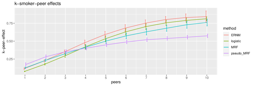
Figure 3: Plot comparing the posteriors distribution of the ERNM, MRF and logistic regression estimated k-peer outcome effect. The MRF with parameters equal to the maximum pseduo likelihood esimtate is also shown

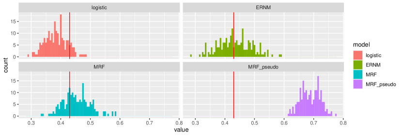
Figure 4: Distribution of proportion of triads with all nodes smokers. ERNM and MRF posterior simulated distributions fit the observed data considerably better that logistic regression or the pseudo-likelihood estimated MRF.

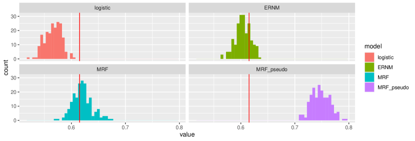
Figure 5: Distribution of proportion edges with both nodes smokers. ERNM and MRF posterior simulated distributions fit the observed data considerably better that logistic regression or the pseudo-likelihood estimated MRF.

8 Discussion

In this paper we model causality when the underlying population is networked and that network endogenous to the social process. Our approach jointly stochastically models the links and nodal covariates in the network, better representing our state of knowledge and their codependency.

Considering a DAG, we suggest that the estimating true causal effects in this setting, is almost always intractable due to the usual lack of fine grained temporal data, as well as the highly complex causal structure. We present a chain graph approximation to the DAG, which allows for a dependence structure that we believe to be compatible with such problems. We then frame the approximate causal inference in terms of network equilibrium potential outcomes, that is, potential outcomes that are free to depend on nodes in the neighbourhood of the node in question. We propose the use of ERNMs to jointly model both random edges and nodal covariates. We also develop a simple modification to the exchange algorithm allowing for a feasible sampling from the posterior distribution. We use the posterior distribution, through simulation, to impute the distribution of the missing potential outcomes, allowing the consideration of the distribution of the causal estimands. We showed, using a school network from the National Longitudinal Study of Adolescent Health, that failing to account for the network structure of the problem could lead to misleading qualitative conclusions, in particular when considering the one- and two- peer outcome effect.

Our primary contributions lie in considering the consequences of relaxing of the commonly made fixed network assumption and proposing the use of suitable social network models to estimate causal effects. This relaxation complicates the causal structure considerably and necessitates the use of complex models to derive causal estimands. Clearly the relaxation of this assumption also allows for greater generalizability. Our inferences hold for the given node set and social process, whereas assuming the fixed network narrows the scope to that observed network only. Our method is only applicable to the given node set. However we suggest that the posteriors derived from the given network can serve as strong priors for “similar” networks. In general, qualitative features of the posteriors from the given network can useful inform other analyses. It is not possible to make further statements than this for networks of different sizes.

We believe that in the context of social network analysis, where individual attributes are heavily influenced by social context, such covariation of edges and nodal covariates is overwhelmingly more representative of many social processes. That is, in many social networks we believe it highly likely that individual characteristics and the connections that form between individuals are strongly dependent. This is especially true if the network evolves over time. We also note that avoiding such issues by letting the size of the network become large and invoking asymptotic arguments, fundamentally mis-interprets the problem. The phenomenon of interest; the inter dependencies of actors, is a result of the small size of the network, for example dependence assumptions implicitly made in modelling a $30$ node network usually do not make sense to apply to say a network of $3000$ nodes. Thus arguments that rely on the number of nodes being large, are incoherent, as they rely on changing the structure of the problem itself, to understand uncertainty. As our approach is fully Bayesian on the fixed node set, we do not require asymptotic arguments on the number of nodes in a network.

Notable by its absence is discussion of suitable prior distributions for ERNMs. We note there has been some work developing conjugate prior distributions for ERGMs (Wang, 2011) and strongly suspect that such an approach may also be applicable in our setting. In practice flat Gaussian prior are often used for ERGMs (Caimo and Friel, 2011). For the purpose of demonstrating our approach, we used uniform priors, which make no account for the geometry of exponential families, but allow us defer careful consideration of possible priors to future work, while demonstrating the utility of our method. We note that we performed similar posterior fits with flat Gaussian priors, which did not effect the posteriors substantially.

The cost of our approach is the strong assumption that such a complex process, can be adequately modelled by an ERNM. This is in general the main criticism of model based causal inference approaches, that models are mis-specified with unknown consequences. In a network setting this mis-specification is often acute e.g. constant marginal effect of additional smoker friends in the linear potential outcomes model. Our central argument is that a complex model is much less mis-specified than current approaches. We have sought to justify this with real data and simulations, though propose this as a future area of research. For example, how dependent do outcomes in networks need to be to invalidate conclusions made with unrealistic models?

The mis-specification may seem to be cause for pessimism, however we emphasize that network settings are indeed the extreme case of small data, as we usually only have one observations of a network on a fixed set of nodes. Thus intuitively we should expect strict functional form assumptions to be required to generate any meaningful statistical, and especially causal inference. In fact we argue that approaching network problems with simpler assumptions is problematic, whilst potentially less prone to mis-specification in the sense that simple models can be used, this easily glosses over the inherent difficulty of dealing with network data where nodes and edges are strongly dependent on other nodes and edges.

we also note that specifying a model for the full network data generation process also allows inference in cases where only a subset of the network is sampled. Accounting for such sampling structure is likely analogous to the method for ERGMs in Gile and Handcock (2016). Accounting for this is not possible with the other methods considered in this work. In addition the network process can be considered to evolve after treatment conditional on some pre treatment network. Such an approach may lead to increased power, for randomised control trials on a networked population, at the cost of our modelling assumptions.

We believe that meaningful steps can be made towards causal inference on networks, through careful consideration of the complex causal structure of such problems. Whilst we make strict assumption on the function form of this, if the researcher is unwilling to make such assumptions, we opine casual inference is out of reach. We suggest it is better to acknowledge the complexity of the situation, and therefore claim that causal inference is not possible, than employing highly restrictive assumptions on the dependence structure of the data generating process, to allow simpler models to be employed.

9 Acknowledgements

This article is based upon work supported by the National Science Foundation(NSF, MMS-0851555, SES-1357619, IIS-1546259) and National Institute of Child Health and Human Development (NICHD, R21HD063000, R21HD075714 and R24-HD041022). The content is solely the responsibility of the authors and do not necessarily represent the official views of the National Institutes of Health or the National Science Foundation.

10 Supplementary Materials

Supplement

The supplement contains an additional chain graph approximation diagram, a review of ERNM and Bayesian computation for them as well as an MCMC convergence analysis for the adolescent health network. (pdf)

References

- Aronow and Samii (2017) Aronow, P. M. and C. Samii (2017, 12). Estimating average causal effects under general interference, with application to a social network experiment. Ann. Appl. Stat. 11(4), 1912–1947.
- Caimo and Friel (2011) Caimo, A. and N. Friel (2011). Bayesian inference for exponential random graph models. Social Networks 33(1), 41 – 55.
- Christakis and Fowler (2007) Christakis, N. A. and J. H. Fowler (2007). The spread of obesity in a large social network over 32 years. New England Journal of Medicine 357(4), 370–379. PMID: 17652652.
- Christakis and Fowler (2008) Christakis, N. A. and J. H. Fowler (2008). The collective dynamics of smoking in a large social network. New England Journal of Medicine 358(21), 2249–2258. PMID: 18499567.
- Christakis and Fowler (2010) Christakis, N. A. and J. H. Fowler (2010, 09). Social network sensors for early detection of contagious outbreaks. PLOS ONE 5(9), 1–8.
- DeAmour (2016) DeAmour, A. (2016). Misspecification, Sparsity, and Superpopulation Inference for Sparse Social Networks. Ph. D. thesis, Harvard University.
- Duijn et al. (2009) Duijn, M., K. Gile, and M. Handcock (2009, 01). A framework for the comparison of maximum pseudo likelihood and maximum likelihood estimation of exponential family random graph models. Social networks 31, 52–62.
- Efron (1979) Efron, B. (1979). Bootstrap Methods: Another Look at the Jackknife. The Annals of Statistics 7(1), 1 – 26.