Extending the Patra–Sen Approach to Estimating the Background Component in a Two-Component Mixture Model

Abstract

Patra and Sen (2016) consider a two-component mixture model, where one component plays the role of background while the other plays the role of signal, and propose to estimate the background component by simply ‘maximizing’ its weight. While in their work the background component is a completely known distribution, we extend their approach here to three emblematic settings: when the background distribution is symmetric; when it is monotonic; and when it is log-concave. In each setting, we derive estimators for the background component, establish consistency, and provide a confidence band. While the estimation of a background component is straightforward when it is taken to be symmetric or monotonic, when it is log-concave its estimation requires the computation of a largest concave minorant, which we implement using sequential quadratic programming. Compared to existing methods, our method has the advantage of requiring much less prior knowledge on the background component, and is thus less prone to model misspecification. We illustrate this methodology on a number of synthetic and real datasets.

1 Introduction

1.1 Two component mixture models

Among mixture models, two-component models play a special role. In robust statistics, they are used to model contamination, with the main component representing the inlier distribution, while the remaining component representing the outlier distribution (Hettmansperger and McKean, 2010; Huber and Ronchetti, 2009; Tukey, 1960; Huber, 1964). In that kind of setting, the contamination is a nuisance and the goal is to study how it impacts certain methods for estimation or testing, and also to design alternative methods that behave comparatively better in the presence of contamination.

In multiple testing, the background distribution plays the role of the distribution assumed (in a simplified framework) to be common to all test statistics under their respective null hypotheses, while the remaining component plays the role of the distribution assumed of the test statistics under their respective alternative hypotheses (Efron et al., 2001; Genovese and Wasserman, 2002). In an ideal situation where the $p$-values can be computed exactly and are uniformly distributed on $[0,1]$ under their respective null hypotheses, the background distribution is the uniform distribution on $[0,1]$. Compared to the contamination perspective, here the situation is in a sense reverse, as we are keenly interested in the component other than the background component. We adopt this multiple testing perspective in the present work.

1.2 The Patra–Sen approach

Working within the multiple testing framework, Patra and Sen (2016) posed the problem of estimating the background component as follows. They operated under the assumption that the background distribution is completely known — a natural choice in many pracical situations, see for example the first two situations in Section 2.3. Given a density $f$ representing the density of all the test statistics combined, and letting $g_{0}$ denote a completely known density, define

$$\theta_{0}:=\sup\{t:f\geq tg_{0}\}.$$ (1)

Note that $\theta_{0}\in[0,1]$. Under some mild assumptions on $f$, the supremum is attained, so that $f$ can be expressed as the following two-component mixture:

$$f=\theta_{0}g_{0}+(1-\theta_{0})u,$$ (2)

for some density $u$. Patra and Sen (2016) aim at estimating $\theta_{0}$ defined in (1) based on a sample from the density $f$, and implement a slightly modified plug-in approach. Even in this relatively simple setting where the background density — the completely known density $g_{0}$ above — is given, information on $\theta_{0}$ can help improve inference in a multiple testing situation as shown early on by Storey (2002), and even earlier by Benjamini and Hochberg (2000).

1.3 Our contribution

We find the Patra–Sen approach elegant, and in the present work extend it to settings where the background distribution (also referred to as the null distribution) — not just the background proportion — is unknown. For an approach that has the potential to be broadly applicable, we consider three emblematic settings where the background distribution is in turn assumed to be symmetric (Section 2), monotone (Section 3), or log-concave (Section 4). Each time, we describe the estimator for the background component (proportion and density) that the Patra-Sen approach leads to, and study its consistency and numerical implementation. We also provide a confidence interval for the background proportion and a simultaneous confidence band for the background density. In addition, in the log-concave setting, we provide a way of computing the largest concave minorant. We address the situation where the background is specified incorrectly, and mention other extensions, including combinations of these settings and in multivariate settings, in Section 5.

1.4 More related work in multiple testing

The work of Patra and Sen (2016) adds to a larger effort to estimate the proportion and/or the density of the null component in a multiple testing scenario. This effort dates back, at least, to early work on false discovery control (Benjamini and Hochberg, 1995) where (over-)estimating the proportion of null hypotheses is crucial to controlling the FDR and related quantities (Storey, 2002; Benjamini and Hochberg, 2000; Genovese and Wasserman, 2004).

Directly focusing on the estimation of the null proportion, Langaas et al. (2005) consider a setting where the $p$-values are uniform in $[0,1]$ under their null hypotheses and have a monotone decreasing density under their alternative hypotheses, while Meinshausen and Rice (2006) do not assume anything of the alternative distribution and propose an estimator which is similar in spirit to that of Patra and Sen (2016). Jin and Cai (2007) and Jin (2008) consider a Gaussian mixture model and approach the problem via the characteristic function — a common approach in deconvolution problems. Gaussian mixtures are also considered in (Efron, 2007, 2012; Cai and Jin, 2010), where the Gaussian component corresponding to the null has unknown parameters that need to be estimated.

Some references to estimating the null component that have been or could be applied in the context of multiple testing are given in (Efron, 2012, Ch 5). Otherwise, we are also aware of the very recent work of Roquain and Verzelen (2020), where in addition to studying the ‘cost’ of having to estimate the parameters of the null distribution when assumed Gaussian, also consider the situation where null distribution belongs to a given location family, and further, propose to estimate the null distribution under an upper bound constraint on the proportion of non-nulls in the mixture model.

Remark 1.

Much more broadly, all this connects with the vast literature on Gaussian mixture models (Cohen, 1967; Lindsay and Basak, 1993) and on mixture models in general (McLachlan and Peel, 2004; McLachlan and Basford, 1988; McLachlan et al., 2019; Lindsay, 1995), including two-component models (Shen et al., 2018; Bordes et al., 2006; Ma and Yao, 2015; Gadat et al., 2020).

2 Symmetric background component

We start with what is perhaps the most natural nonparametric class of null distributions: the class of symmetric distributions about the origin. Unlike Roquain and Verzelen (2020), who assume that the null distribution is symmetric around an unknown location that needs to be estimated but is otherwise known, i.e., its ‘shape’ is known, we assume that the shape is unknown. We do assume that the center of symmetry is known, but this is for simplicity, as an extension to an unknown center of symmetry is straightforward (see our numerical experiments in Section 2.2). Mixtures of symmetric distributions are considered in (Hunter et al., 2007), but otherwise, we are not aware of works estimating the null distribution under an assumption of symmetry in the context of multiple testing. For works in multiple testing that assume that the null distribution is symmetric but unknown, but where the goal is either testing the global null hypothesis or controlling the false discovery rate, see (Arias-Castro and Wang, 2017; Arias-Castro and Chen, 2017).

Following the footsteps of Patra and Sen (2016), we make sense of the problem by defining for a density $f$ the following:

$$\pi_{0}:=\sup\big{\{}\pi:\exists g\in\mathcal{S}\text{ s.t. }f-\pi g\geq 0\text{ a.e.}\big{\}},$$ (3)

where $\mathcal{S}$ is the class of even densities (i.e., representing a distribution that is symmetric about the origin). Note that $\pi_{0}\in[0,1]$ is well-defined for any density $f$, with $\pi_{0}=1$ if and only if $f$ itself is symmetric.

Theorem 1.

We have

$$\pi_{0}=\int_{-\infty}^{\infty}h_{0}(x)dx, h_{0}(x):=\min\{f(x),f(-x)\}.$$ (4)

Moreover, if $\pi_{0}>0$ the supremum in (3) is attained by the following density and no other  :

$$g_{0}(x):=\frac{h_{0}(x)}{\pi_{0}}.$$ (5)

Proof.

The parameter $\pi_{0}$ can be equivalently defined as

$$\pi_{0}=\sup\big{\{}\textstyle\int h:\text{$h$ is even and $0\leq h\leq f$ a.e.}\big{\}}.$$ (6)

Note that $h_{0}$, as defined in the statement, satisfies the above conditions, implying that $\pi_{0}\geq\int h_{0}$. Take $h$ satisfying these same conditions, namely, $h(x)=h(-x)$ and $0\leq h(x)\leq f(x)$ for almost all $x$. Then, for almost any $x$, $h(x)\leq f(x)$ and $h(-x)\leq f(-x)$, implying that $h(x)\leq f(x)\wedge f(-x)=h_{0}(x)$. (Here and elsewhere, $a\wedge b$ is another way of denoting $\min(a,b)$.) Hence, $\int h\leq\int h_{0}$ with equality if and only if $h=h_{0}$ a.e., in particular implying that $\pi_{0}\leq\int h_{0}$. We have thus established that $\pi_{0}=\int h_{0}$, and also that $\int h=\pi_{0}$ if and only if $h=h_{0}$ a.e.. This not only proves (4), but also (5), essentially by definition. ∎

We have thus established that, in the setting of this section, the background component as defined above is given by

$$h_{0}(x)=\pi_{0}g_{0}(x)=\min\{f(x),f(-x)\},$$ (7)

and $f$ can be expressed as a mixture of the background density and another, unspecified, density $u$, as follows:

$$f=\pi_{0}g_{0}+(1-\pi_{0})u.$$ (8)

The procedure is summarized in Table 1. An illustration of this decomposition is shown in Figure 1. By construction, the density $u$ is such that it has no symmetric background component in that, for almost every $x$, $u(x)=0$ or $u(-x)=0$.

Table 1: Symmetric background computation.

inputs: density ${f}$, given center of symmetry $c_{0}$ or candidate center points $\{c_{1},c_{2},\dots,c_{k}$}
if center of symmetry is not provided then for $i=1,\dots,k$ do $h_{i}(x)=\min\{{f}(x),{f}(2c_{i}-x)\}$ $\pi_{i}(x)=\int_{-\infty}^{\infty}h_{i}(x)dx$ $\beta=\operatorname*{arg\,max}_{i}\pi_{i}(x)$ $c_{0}=c_{\beta}$ $h_{0}(x)=\min\{{f}(x),{f}(2c_{0}-x)\}$ $\pi_{0}=\int_{-\infty}^{\infty}h_{0}(x)dx$ $g_{0}(x)=h_{0}(x)/\pi_{0}$
return $c_{0},\pi_{0},g_{0},h_{0}$

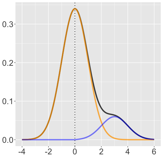
(a) Decomposition of $f$ with center of symmetry specified as $0$ (dotted).

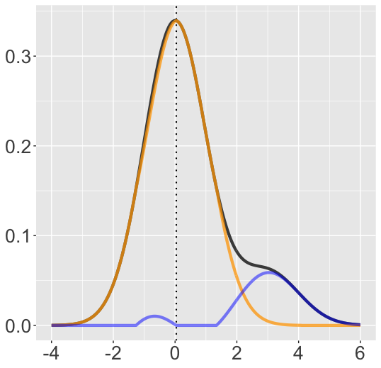
(b) Decomposition of $f$ with center of symmetry, $0.04$ (dotted), found by maximization.

Figure 1: The density $f$ of the Gaussian mixture $0.85\text{ }\mathcal{N}(0,1)+0.15\text{ }\mathcal{N}(0,1)$, in black, and its decomposition into $\pi_{0}g_{0}$, in orange, and $(1-\pi_{0})u$, in blue. We specify the center of symmetry as $0$ on the left, and we do not specify the center of symmetry on the right. Notice $\pi_{0}=0.850$ on the left and $\pi_{0}=0.860$ on the right.

2.1 Estimation and consistency

When all we have to work with is a sample — $x_{1},x_{2},\dots,x_{n}\in\mathbb{R}$ — we adopt a straightforward plug-in approach: We estimate the density $f$, obtaining $\hat{f}$, and apply the procedure of Table 1, meaning, we compute $\hat{h}_{0}(x):=\min\{\hat{f}(x),\hat{f}(-x)\}$. If we want estimates for the background density and proportion, we simply return $\hat{\pi}_{0}:=\int\hat{h}_{0}$ and $\hat{g}_{0}:=\hat{h}_{0}/\hat{\pi}_{0}$. (By convention, we set $\hat{g}_{0}$ to the standard normal distribution if $\hat{\pi}_{0}=0$.)

We say that $\hat{f}=\hat{f}_{n}$ is locally uniformly consistent for $f$ if $\operatorname{\mathbb{E}}[\operatorname*{ess\,sup}_{x\in I}|\hat{f}_{n}(x)-f(x)|]\to 0$ as $n\to\infty$ for any bounded interval $I$. (Here and elsewhere, $\operatorname*{ess\,sup}_{x\in I}f(x)$ denotes the essential supremum of $f$ over the set $I$.) We note that this consistency condition is satisfied, for example, when $f$ is continuous and $\hat{f}$ is the kernel density estimator with the Gaussian kernel and bandwidth chosen by cross-validation (Chow et al., 1983).

Theorem 2.

Suppose that $\hat{f}$ is a true density and locally uniformly consistent for $f$. Then $\hat{h}_{0}$ is locally uniformly consistent for $h_{0}$ and $\hat{\pi}_{0}$ is consistent, and if $\pi_{0}>0$, then $\hat{g}_{0}$ is locally uniformly consistent for $g_{0}$.

Proof.

All the limits that follows are as the sample size diverges to infinity. We rely on the elementary fact that, for $a_{1},a_{2},b_{1},b_{2}\in\mathbb{R}$,

$$\big{|}\min\{a_{1},b_{1}\}-\min\{a_{2},b_{2}\}\big{|}\leq\max\{|a_{1}-a_{2}|,|b_{1}-b_{2}|\},$$ (9)

to get that, for all $x$,

$$|\hat{h}_{0}(x)-h_{0}(x)|\leq\max\{|\hat{f}(x)-f(x)|,|\hat{f}(-x)-f(-x)|\},$$ (10)

implying that $\hat{h}_{0}$ is locally uniformly consistent for $h_{0}$. To be sure, take a bounded interval $I$, which we assume to be symmetric without loss of generality. Then

$$\operatorname*{ess\,sup}_{x\in I}|\hat{h}_{0}(x)-h_{0}(x)| \leq\operatorname*{ess\,sup}_{x\in I}|\hat{f}(x)-f(x)|\vee\operatorname*{ess\,sup}_{x\in I}|\hat{f}(-x)-f(-x)|$$

$$=\operatorname*{ess\,sup}_{x\in I}|\hat{f}(x)-f(x)|,$$

and we then use the fact that $\operatorname{\mathbb{E}}[\operatorname*{ess\,sup}_{I}|\hat{f}-f|]\to 0$. (Here and elsewhere, $a\vee b$ is another way of denoting $\max(a,b)$.)

To conclude, it suffices to show that $\hat{\pi}_{0}$ is consistent for $\pi_{0}$. Fix $\varepsilon>0$ arbitrarily small. There is a bounded interval $I$ such that $\int_{I}f\geq 1-\varepsilon$. Then, by the fact that $0\leq h_{0}\leq f$ a.e.,

$$\int_{I}h_{0}\leq\pi_{0}=\int h_{0}\leq\int_{I}h_{0}+\int_{I^{\mathsf{c}}}f\leq\int_{I}h_{0}+\varepsilon.$$

($I^{\mathsf{c}}$ denotes the complement of $I$, meaning, $I^{\mathsf{c}}=\mathbb{R}\setminus I$.) Similarly, by the fact that $0\leq\hat{h}_{0}\leq\hat{f}$ a.e.,

$$\int_{I}\hat{h}_{0}\leq\hat{\pi}_{0}=\int\hat{h}_{0}\leq\int_{I}\hat{h}_{0}+\int_{I^{\mathsf{c}}}\hat{f}.$$

From this we gather that

$$\int_{I}\hat{h}_{0}-\int_{I}h_{0}-\varepsilon\leq\hat{\pi}_{0}-\pi_{0}\leq\int_{I}\hat{h}_{0}-\int_{I}h_{0}+\int_{I^{\mathsf{c}}}\hat{f}.$$

Thus consistency of $\hat{\pi}_{0}$ follows if we establish that $\limsup\int_{I^{\mathsf{c}}}\hat{f}\leq\varepsilon$ and that $\int_{I}\hat{h}_{0}-\int_{I}h_{0}\to 0$. The former comes from the fact that

$$\int_{I^{\mathsf{c}}}\hat{f} =\int_{I^{\mathsf{c}}}\hat{f}-\int_{I^{\mathsf{c}}}f+\int_{I^{\mathsf{c}}}f$$

$$\leq\int_{I}(\hat{f}-f)+\varepsilon$$

$$\leq|I|\operatorname*{ess\,sup}_{I}|\hat{f}-f|+\varepsilon\to\varepsilon,$$

using the fact that $f$ and $\hat{f}$ are densities and that $\int_{I^{\mathsf{c}}}f\leq\varepsilon$. ($|I|$ denotes the Lebesgue measure of $I$, meaning its length when $I$ is an interval.) For the latter, we have

$$\left|\int_{I}\hat{h}_{0}-\int_{I}h_{0}\right| \leq\int_{I}|\hat{h}_{0}-h_{0}| \leq|I|\operatorname*{ess\,sup}_{I}|\hat{h}_{0}-h_{0}|\to 0,$$

having already established that $\hat{h}_{0}$ is locally uniformly consistent for $h_{0}$. ∎

Confidence interval and confidence band

Beyond mere pointwise consistency, suppose that we have available a confidence band for $f$, which can be derived under some conditions on $f$ from a kernel density estimator — see (Chen, 2017) or (Giné and Nickl, 2021, Ch 6.4).

Theorem 3.

Suppose that for some $\alpha\in(0,1)$, we have at our disposal $\hat{f}_{l}$ and $\hat{f}_{u}$ such that

$$\operatorname{\mathbb{P}}\big{(}\hat{f}_{l}(x)\leq f(x)\leq\hat{f}_{u}(x),\text{ for almost all $x$}\big{)}\geq 1-\alpha.$$ (11)

Then, with probability at least $1-\alpha$,

$$\hat{\pi}_{l}\leq\pi_{0}\leq\hat{\pi}_{u}, \hat{g}_{l}\leq g_{0}\leq\hat{g}_{u}\text{ a.e.},$$ (12)

where

$$\hat{\pi}_{l}:=\int\hat{h}_{l}, \hat{\pi}_{u}:=\int\hat{h}_{u}, \hat{h}_{l}(x):=\min\{\hat{f}_{l}(x),\hat{f}_{l}(-x)\}, \hat{h}_{u}(x):=\min\{\hat{f}_{u}(x),\hat{f}_{u}(-x)\}.$$

Proof.

Let $\Omega$ be the event that $\hat{f}_{l}(x)\leq f(x)\leq\hat{f}_{u}(x)$ for almost all $x$, and note that $\operatorname{\mathbb{P}}(\Omega)\geq 1-\alpha$ by assumption. Assuming that $\Omega$ holds, we have, for almost all $x$,

$$\hat{f}_{l}(x)\leq f(x)\leq\hat{f}_{u}(x), \hat{f}_{l}(-x)\leq f(-x)\leq\hat{f}_{u}(-x),$$

and taking the minimum in the corresponding places yields

$$\hat{h}_{l}(x)\leq h_{0}(x)\leq\hat{h}_{u}(x).$$ (13)

Everything else follows immediately from this. ∎

In words, we apply the procedure of Table 1 to the lower and upper bounds, $\hat{f}_{l}$ and $\hat{f}_{u}$. If the center of symmetry is not provided, then we determine it based on $\hat{f}$, and then use that same center for $\hat{f}_{l}$ and $\hat{f}_{u}$.

2.2 Numerical experiments

In this subsection we provide simulated examples when the background distribution is taken to be symmetric. We acquire $\hat{f}$ by kernel density estimation using the Gaussian kernel with bandwidth selected by cross-validation (Rudemo, 1982; Stone, 1984; Arlot and Celisse, 2010; Silverman, 1986; Sheather and Jones, 1991), where the cross-validated bandwidth selection is implemented in the kedd package (Guidoum, 2020). The consistency of this density estimator has been proven in (Chow et al., 1983). Although there are many methods that provide confidence bands for kernel density estimator, for example (Bickel and Rosenblatt, 1973; Giné and Nickl, 2010), for consideration of simplicity and intuitiveness, our simultaneous confidence band (in the form of $\hat{f}_{l}$ and $\hat{f}_{u}$) used in the experiments is acquired from bootstrapping a debiased estimator of the density as proposed in (Cheng and Chen, 2019). For a comprehensive review on the area of kernel density and confidence bands, we point the reader to the recent survey paper (Chen, 2017) and textbook (Giné and Nickl, 2021, Ch 6.4).

In the experiments below, we carry out method and report the estimated proportion $\hat{\pi}_{0}$, as well as its $95\%$ confidence interval $(\hat{\pi}_{0}^{\rm{L}},\hat{\pi}_{0}^{\rm{U}})$. We consider both the situation where the center of symmetry is given, and the situation where it is not. In the latter situation, we also report the background component’s estimated center, which is selected among several candidate centers and chosen as the one giving the largest symmetric background proportion.

We are not aware of other methods for estimating the quantity $\pi_{0}$, but we provide a comparison with several well-known methods that estimate similar quantities. To begin with, we consider the method of Patra and Sen (2016), which estimates the quantity $\theta_{0}$ as defined in $\eqref{theta_0_definition}$. We let $\hat{\theta}_{0}^{\rm{PSC}}$, $\hat{\theta}_{0}^{\rm{PSH}}$, $\hat{\theta}_{0}^{\rm{PSB}}$ denote the constant, heuristic, and $95\%$ upper bound estimator on $\theta_{0}$, respectively. We then consider estimators of the quantity $\theta$, the actual proportion of the given background component $f_{b}$ in the mixture density

$$f=\theta f_{b}+(1-\theta)u,$$ (14)

where $u$ denotes the unknown component. Note that $\theta_{0}$ and $\pi_{0}$ may be different from $\theta$. This mixture model may not be identifiable in general, and we discuss this issue down below. We also consider the estimator of (Efron, 2007), denoted $\hat{\theta}^{\rm{E}}$, and implemented in package locfdr . This method requires the unknown component to be located away from $0$, and to be have heavier tails than the background component. In addition, when the $p$-values are known, Meinshausen and Rice (2006) provide a $95\%$ upper bound on the proportion of the null component, and we include that estimator also, denoted $\hat{\theta}^{\rm{MR}}$, and implemented in package howmany . Finally, when the distribution is assumed to be a Gaussian mixture, Cai and Jin (2010) provide an estimator, denoted $\hat{\theta}^{\rm{CJ}}$, when the unknown component is assumed to have larger standard deviation than the background component. $\hat{\theta}^{\rm{CJ}}$ requires the specification of a parameter $\gamma$, and following the advice given by the authors, we select $\gamma=0.2$. Importantly, unlike our method, these other methods assume knowledge of the background distribution. (Note that the methods of Efron (2007) and Cai and Jin (2010) do not necessitate full knowledge of the background distribution, but we provide them with that knowledge in all the simulated datasets.) We summarize the methods used in our experiments in Table 2. For experiments in situations where the background component is misspecified, we invite the reader to Section 5.1.

Table 2: Summary of the methods considered in our experiments.

Estimator	Reference	Description	Background information needed
$\hat{\pi}_{0},\hat{\pi}_{0}^{\rm{L}},\hat{\pi}_{0}^{\rm{U}}$	Current paper	Estimator of $\pi_{0}$ with $95\%$ lower and upper confidence bounds.	Requires background distribution to be symmetric (note the requirement becomes monotonic in Section 3 or log-concave in Section 4).
$\hat{\theta}_{0}^{\rm{PSC}},\hat{\theta}_{0}^{\rm{PSH}},\hat{\theta}_{0}^{\rm{PSB}}$	(Patra and Sen, 2016)	Constant, heuristic, and $95\%$ upper bound estimates of $\theta_{0}$.	Requires complete knowledge on the background distribution.
$\hat{\theta}_{0}^{\rm{E}}$	(Efron, 2007)	Estimator of $\theta$.	Either requires full knowledge of background distribution or can estimate the background distribution when it has shape similar to a Gaussian distribution centered around $0$.
$\hat{\theta}_{0}^{\rm{MR}}$	(Meinshausen and Rice, 2006)	$95\%$ upper bound of $\theta$.	Requires complete knowledge on the background distribution.
$\hat{\theta}_{0}^{\rm{CJ}}$	(Cai and Jin, 2010)	Estimator of $\theta$.	Either requires full knowledge of background distribution or can estimate the background distribution when it is Gaussian.

We consider four different situations as listed in Table 3. Each situation’s corresponding $\theta$, $\theta_{0}$, and $\pi_{0}$, defined as in (3), are also presented, where $\theta_{0}$ and $\pi_{0}$ are obtained numerically based on knowledge of $f$. For each model, we generate a sample of size $n=1000$ and compute all the estimators described above. We repeat this process $1000$ times. We transform the data accordingly when applying the comparison methods. The result of our experiment are reported, in terms of the mean values as well as standard deviations, in Table 4. It can be seen that in most situations, our estimator achieves comparable if not better performance when estimating $\pi_{0}$ as compared to the other methods for the parameter they are meant to estimate ($\theta$ or $\theta_{0}$). We also note that our method is significantly influenced by the estimation of $\hat{f}$, therefore in situations where $\hat{f}$ deviates from $f$ often, our estimator will likely result in higher error. In addition, it is clear from the experiments that specifying the center of symmetry is unnecessary.

Table 3: Simulated situations for the estimation of a symmetric background component, together with the corresponding values of $\theta$, $\theta_{0}$, $\pi_{0}$ (unspecified center), and $\pi_{00}$ (given center), obtained numerically (and rounded at 3 decimals).

Model	Distribution	$\theta$	$\theta_{0}$	$\pi_{0}$	$\pi_{00}$
S1	$0.85\text{ }\mathcal{N}(0,1)+0.15\text{ }\mathcal{N}(3,1)$	0.850	0.850	0.860	0.850
S2	$0.95\text{ }\mathcal{N}(0,1)+0.05\text{ }\mathcal{N}(3,1)$	0.950	0.950	0.950	0.950
S3	$0.85\text{ }\mathcal{N}(0,1)+0.1\text{ }\mathcal{N}(2.5,0.75)+0.05\text{ }\mathcal{N}(-2.5,0.75)$	0.850	0.851	0.954	0.950
S4	$0.85\text{ }\mathcal{N}(0,1)+0.1\text{ }\mathcal{N}(2.5,0.75)+0.05\text{ }\mathcal{N}(5,0.75)$	0.850	0.850	0.858	0.850

Table 4: A comparison of various methods for estimating a background component in the situations of Table 3. For our method, the first and second rows in each situation are for when the center is unspecified, while the third and fourth rows are for when the center is specified to be the origin. Thus $\hat{\pi}_{0}$ on the first row of each situation is compared with $\pi_{0}$, $\hat{\pi}_{0}$ on the third row of each situation is compared with $\pi_{00}$. Otherwise, the $\hat{\theta}_{0}^{\rm X}$ are compared with $\theta_{0}$, while the $\hat{\theta}^{X}$ are compared with $\theta$.

Model	Center	$\hat{\pi}_{0}$	$\hat{\pi}_{0}^{\rm{L}}$	$\hat{\pi}_{0}^{\rm{U}}$	Null	$\hat{\theta}_{0}^{\rm{PSC}}$	$\hat{\theta}_{0}^{\rm{PSH}}$	$\hat{\theta}_{0}^{\rm{PSB}}$	$\hat{\theta}^{\rm{E}}$	$\hat{\theta}^{\rm{MR}}$	$\hat{\theta}^{\rm{CJ}}$
S1	0.068	0.857	0.571	1	$\mathcal{N}(0,1)$	0.848	0.855	0.893	0.861	0.890	0.893
	(0.052)	(0.021)	(0.059)	(0)		(0.024)	(0.023)	(0.018)	(0.023)	(0.014)	(0.085)
	0	0.835	0.561	1
	given	(0.022)	(0.058)	(0)
S2	0.024	0.936	0.631	1	$\mathcal{N}(0,1)$	0.938	0.954	0.985	0.955	0.972	0.963
	(0.044)	(0.017)	(0.066)	(0)		(0.023)	(0.022)	(0.015)	(0.026)	(0.008)	(0.082)
	0	0.925	0.623	1
	given	(0.019)	(0.067)	(0)
S3	0.046	0.945	0.597	1	$\mathcal{N}(0,1)$	0.864	0.942	0.937	0.856	0.896	0.707
	(0.050)	(0.019)	(0.063)	(0)		(0.023)	(0.034)	(0.017)	(0.024)	(0.015)	(0.085)
	0	0.930	0.587	1
	given	(0.020)	(0.064)	(0)
S4	0.070	0.856	0.574	1	$\mathcal{N}(0,1)$	0.846	0.854	0.891	0.849	0.889	0.713
	(0.056)	(0.021)	(0.061)	(0)		(0.023)	(0.024)	(0.018)	(0.024)	(0.014)	(0.088)
	0	0.833	0.563	1
	given	(0.022)	(0.060)	(0)

2.3 Real data analysis

In this subsection we examine six real datasets where the null component could be reasonably assumed to be symmetric.

We begin with two datasets where we have sufficient information on the background component. The first one is the Prostate dataset (Singh et al., 2002), which contains gene expression levels for $n=6033$ genes on $102$ men, $50$ of which are control subjects and $52$ are prostate cancer patients. The main objective is to discover the genes that have a different expression level on the control and prostate patient groups. For each gene, we conduct a two-sided two sample $t$ test on the control subjects and prostate patients, and then transform these $t$ statistics into $z$ values, using

$$z_{i}=\Phi^{-1}(F_{100}(t_{i})),\text{ }i=1,2,\dots,6033,$$ (15)

where $\Phi$ denotes the cdf of the standard normal distribution, and $F_{100}$ denotes the cdf of the $t$ distribution with 100 degrees of freedom. We work with these $n=6033$ $z$ values. From (Efron, 2007) the background component here could be reasonably assumed to be $\mathcal{N}(0,1)$. The results of the different proportion estimators compared in Section 2.2 are shown in the first row of Table 5. The fitted largest symmetric component as well as confidence bands are plotted in Figure 2(a).

Next we consider the Carina dataset (Walker et al., 2007), which contains the radial velocities of $n=1266$ stars in Carina, a dwarf spheroidal galaxy, mixed with those of Milky Way stars in the field of view. As Patra and Sen (2016) stated, the background distribution of the radial velocity, bgstars, can be acquired from (Robin et al., 2003). The various estimators are computed and shown in the second row of Table 5. The fitted largest symmetric component as well as confidence bands are plotted in Figure 2(b).

Table 5: Two real datasets where background component can be reasonably guessed or derived. We compare the same methods for extracting a background symmetric component as in Section 2.2. (Note that we work with $z$ values here instead of $p$-values so our results for the Prostate dataset are slightly different from those reported by Patra and Sen (2016).)

Model	Center	$\hat{\pi}_{0}$	$\hat{\pi}_{0}^{\rm{L}}$	$\hat{\pi}_{0}^{\rm{U}}$	Null	$\hat{\theta}_{0}^{\rm{PSC}}$	$\hat{\theta}_{0}^{\rm{PSH}}$	$\hat{\theta}_{0}^{\rm{PSB}}$	$\hat{\theta}^{\rm{E}}$	$\hat{\theta}^{\rm{MR}}$	$\hat{\theta}^{\rm{CJ}}$
Prostate	0	0.977	0.789	1	$\mathcal{N}(0,1)$	0.931	0.941	0.975	0.931	0.956	0.867
Carina	59	0.540	0.071	1	bgstars	0.636	0.645	0.677	0.951	0.664	0.206

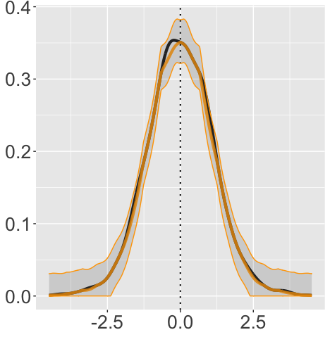
(a) Prostate dataset

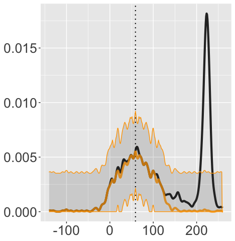
(b) Carina dataset

Figure 2: Estimated symmetric component on the Prostate ($z$ values) and Carina (radial velocity) datasets: the black curve represents the fitted density; the center orange curve represents the computed $\hat{h}_{0}$; the top and bottom orange curves represent the $95\%$ simultaneous confidence bands for $h_{0}$; the estimated center of the symmetric component is indicated by a dotted vertical line.

Aside from these two real datasets where we know the background distribution, we consider four other real datasets — three microarray datasets and one police dataset — where we do not know the null distribution (Efron, 2012). Here, out of the methods considered above, only our method and that of (Efron, 2007) and (Cai and Jin, 2010) are applicable. For the first comparison method we use the MLE estimation as presented in (Efron, 2007, Sec 4), which is usually very close to the result of Central Matching as used in (Efron, 2012). For the second comparison method we use the estimator in (Cai and Jin, 2010, Sec 3.2), although we use $\gamma=0.1$ as the recommended value $\gamma=0.2$ leads to significant underestimation of the background proportion. Note that both of these methods are still meant to estimate $\theta$.

The HIV dataset (van’t Wout et al., 2003) consists of a study of $4$ HIV subjects and $4$ control subjects. The measurements of $n=7680$ gene expression levels were acquired using cDNA microarrays on each subject. We compute $t$ statistics for the two sided $t$ test and then transform them into $z$ values using (15), with the degree of freedom being $6$ here. We would like to know what proportion of these genes do not show a significant difference in expression levels between HIV and control subjects. The results are summarized in the first row of Table 6. The fitted largest symmetric component as well as confidence bands are shown in Figure 3(a).

The Leukemia dataset comes from (Golub et al., 1999). There are $72$ patients in this study, of which $45$ have ALL (Acute Lymphoblastic Leukemia) and $27$ have AML (Acute Myeloid Leukemia), with AML being considered more severe. High density oligonucleotide microarrays gave expression levels on $n=7128$ genes. Following (Efron, 2012, Ch 6.1), the raw expression levels on each microarray, $x_{i,j}$ for gene $i$ on array $j$, were transformed to a normal score

$$y_{i,j}=\Phi^{-1}\bigg{(}\big{(}\textsf{rank}(x_{i,j})-0.5\big{)}/n\bigg{)},$$ (16)

where $\textsf{rank}(x_{i,j})$ denotes the rank of $x_{i,j}$ among $n$ raw values of array $j$. Then $t$ tests were then conducted on ALL and AML patients, and $t$ statistics were transformed to $z$ values according to (15), now with $70$ degrees of freedom. As before, we would like to know the proportion of genes that do not show a significant difference in expression levels between ALL and AML patients. The results are summarized in the second row of Table 6. The fitted largest symmetric component as well as confidence bands are shown in Figure 3(b).

The Parkinson dataset comes from (Lesnick et al., 2007). In this dataset, substantia nigra tissue — a brain structure located in the mesencephalon that plays an important role in reward, addiction, and movement — from postmortem the brain of normal and Parkinson disease patients were used for RNA extraction and hybridization, done on Affymetrix microarrays. In this dataset, there are $n=54277$ nucleotide sequences whose expression levels were measured on $16$ Parkinson’s disease patients and $9$ control patients. We wish to find out the proportion of sequences that do not show significant difference between Parkinson and control patients. The results are summarized in the third row of Table 6. The fitted largest symmetric component as well as confidence bands are shown in Figure 3(c).

The Police dataset is analyzed in (Ridgeway and MacDonald, 2009). In 2006, based on $500000$ pedestrian stops in New York City, each of the city’s $n=2749$ police officers that were regularly involved in pedestrian stops were assigned a $z$ score on the basis of their stop data, in consideration of possible racial bias. For details on computing this $z$ score, we refer the reader to (Ridgeway and MacDonald, 2009; Efron, 2012). Large positive $z$ values are considered as possible evidence of racial bias. We would like to know the percentage of these police officers that do not exhibit a racial bias in pedestrian traffic stops. The estimated proportion are reported on the last row of Table 6. The symmetric component as well as confidence bands are presented in Figure 3(d).

Table 6: Real datasets where background distribution is unknown and needs to be estimated. We compare the methods for extracting a background symmetric component among those in Section 2.2 that apply.

Model	Center	$\hat{\pi}_{0}$	$\hat{\pi}_{0}^{\rm{L}}$	$\hat{\pi}_{0}^{\rm{U}}$	$\hat{\theta}^{\rm{E}}$	$\hat{\theta}^{\rm{CJ}}$
HIV	-0.62	0.950	0.775	1	0.940	0.926
Leukemia	0.16	0.918	0.639	1	0.911	0.820
Parkinson	-0.18	0.985	0.924	1	0.998	0.993
Police	0.10	0.982	0.767	1	0.985	0.978

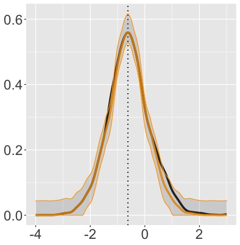
(a) HIV dataset

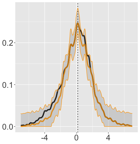
(b) Leukemia dataset

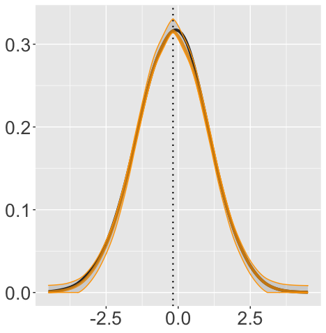
(c) Parkinson dataset

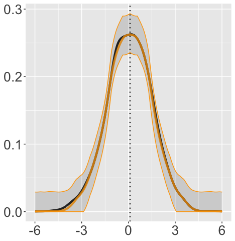
(d) Police dataset

Figure 3: Estimated symmetric component on HIV ($z$ values), Leukemia ($z$ values), Parkinson ($z$ values), and Police ($z$ scores) datasets: the black curve represents the fitted density; the center orange curve represents the computed $\hat{h}_{0}$; the top and bottom orange curves represent the $95\%$ simultaneous confidence bands for $h_{0}$; the estimated center of the symmetric component is indicated by a dotted vertical line.

3 Monotone background component

In this section, we turn our attention to extracting from a density its monotone background component following the Patra–Sen approach. For this to make sense, we only consider densities supported on $\mathbb{R}_{+}=[0,\infty)$. In fact, all the densities we consider in this section will be supported on $\mathbb{R}_{+}$. For such a density $f$, we thus define

$$\pi_{0}:=\sup\big{\{}\pi:\exists g\in\mathcal{M}\text{ s.t. }f-\pi g\geq 0\text{ a.e.}\big{\}},$$ (17)

where $\mathcal{M}$ is the class of monotone (necessarily non-increasing) densities on $\mathbb{R}_{+}$. Note that $\pi_{0}\in[0,1]$ is well-defined for any density $f$, with $\pi_{0}=1$ if and only if $f$ itself is monotone.

Recall that the essential infimum of a measurable set $A$, denoted $\operatorname*{ess\,inf}A$, is defined as the supremum over $t\in\mathbb{R}$ such that $A\cap(-\infty,t)$ has Lebesgue measure zero. Everywhere in this section, we will assume that $f$ is càdlàg, meaning that, at any point, it is continuous from the right and admits a limit from the left.

Theorem 4.

Assuming $f$ is càdlàg, we have

$$\pi_{0}=\int_{0}^{\infty}h_{0}(x)dx, h_{0}(x):=\operatorname*{ess\,inf}\{f(y):y\leq x\}.$$ (18)

Moreover, if $\pi_{0}>0$ the supremum in (17) is attained by the following density and no other:

$$g_{0}(x):=\frac{h_{0}(x)}{\pi_{0}}.$$ (19)

Note that $\pi_{0}=0$ (i.e., $f$ has no monotone background component) if and only if $\operatorname*{ess\,inf}\{f(y):y\leq x\}=0$ for some $x>0$, or equivalently, if $\{x\in[0,t]:f(x)\leq\varepsilon\}$ has positive measure for all $t>0$ and all $\varepsilon>0$. If $f$ is càdlàg, this condition reduces to $f(0)=0$. Also, if $f$ is càdlàg, $h_{0}(x)=\min\{f(y):y<x\}$.

Proof.

Note that $\pi_{0}$ can be equivalently defined as

$$\pi_{0}=\sup\big{\{}\textstyle{\int h}:\text{$h$ is monotone and $0\leq h\leq f$ a.e.}\big{\}}.$$ (20)

Note that $h_{0}$, as defined in the statement, satisfies the above conditions, implying that $\pi_{0}\geq\int h_{0}$. Take $h$ satisfying these same conditions, namely, $h$ is monotone and $0\leq h(x)\leq f(x)$ for almost all $x$, say, for $x\in\mathbb{R}_{+}\setminus A$ where $A$ has Lebesgue measure zero. Take such an $x$. Then for any $y\leq x$ we have $h(x)\leq h(y)$, and $h(y)\leq f(y)$ if in addition $y\notin A$. Hence,

$$h(x)\leq\inf\{f(y):y<x,y\notin A\}\leq\operatorname*{ess\,inf}\{f(y):y<x\}=h_{0}(x),$$

where the second inequality comes from the fact that $A$ has zero Lebesgue measure and the definition of essential infimum. Hence, $\int h\leq\int h_{0}$ with equality if and only if $h=h_{0}$ a.e., in particular implying that $\pi_{0}\leq\int h_{0}$. We have thus established that $\pi_{0}=\int h_{0}$, and also that $\int h=\pi_{0}$ if and only if $h=h_{0}$ a.e.. This not only proves (18), but also (19). ∎

We have thus established that, in the setting of this section where $f$ is assumed to be càdlàg, the background component as defined above is given by

$$h_{0}(x)=\pi_{0}g_{0}(x)=\operatorname*{ess\,inf}\{f(y):y<x\},$$ (21)

and $f$ can be expressed as a mixture of the background density and another, unspecified, density $u$, as follows:

$$f=\pi_{0}g_{0}+(1-\pi_{0})u.$$ (22)

The procedure is summarized in Table 7. An illustration of this decomposition is shown in Figure 4. (In this section, $\mathcal{E}(\sigma)$ denotes the exponential distribution with scale $\sigma$ and $\mathcal{G}(\kappa,\sigma)$ denotes the Gamma distribution with shape $\kappa$ and scale $\sigma$. Recall that $\mathcal{E}(\sigma)\equiv\mathcal{G}(1,\sigma)$.) By construction, the density $u$ is such that it has no monotone background component in that $\operatorname*{ess\,inf}\{u(y):y<x\}=0$ for any $x>0$.

Table 7: Monotone background computation.

inputs: density ${f}$ defined on $[0,\infty)$
$h_{0}(x)=\operatorname*{ess\,inf}\{f(y):y\leq x\}$ $\pi_{0}=\int_{0}^{\infty}h_{0}(x)dx$ $g_{0}(x)=h_{0}(x)/\pi_{0}$
return $\pi_{0},g_{0},h_{0}$

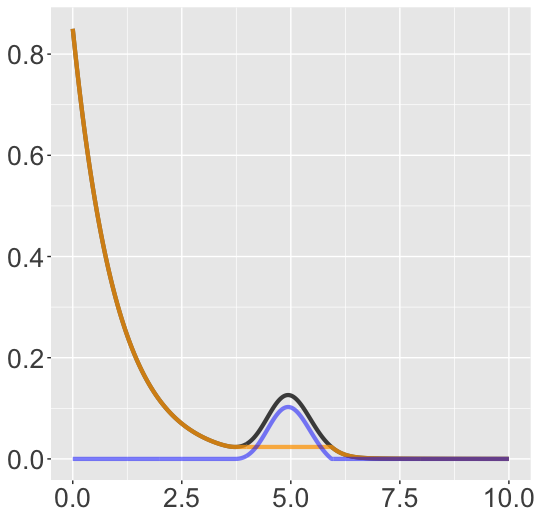
Figure 4: The density $f$ of the Gamma mixture $0.85\text{ }\mathcal{Exp}(1)+0.15\text{ }\mathcal{Gamma}(100,1/20)$, in black, and its decomposition into $\pi_{0}g_{0}$, in orange, and $(1-\pi_{0})u$, in blue. Notice that the orange curve has a flat part around the middle and is slightly different from $0.85\text{ }\mathcal{Exp}(1)$.

3.1 Estimation and consistency

In practice, when all we have is a sample of observations, $x_{1},\dots,x_{n}\in\mathbb{R}_{+}$, we first estimate the density, resulting in $\hat{f}$, and then compute the quantities defined in (18) and (19) with $\hat{f}$ in place of $f$. Thus our estimates are

$$\hat{\pi}_{0}:=\int_{0}^{\infty}\hat{h}_{0}(x)dx, \hat{h}_{0}(x):=\operatorname*{ess\,inf}\{\hat{f}(y):y<x\}, \hat{g}_{0}(x):=\frac{\hat{h}_{0}(x)}{\hat{\pi}_{0}}.$$ (23)

Theorem 5.

Assume $f$ is càdlàg, and suppose that $\hat{f}$ is a true density, càdlàg, and is locally uniformly consistent for $f$. Then $\hat{h}_{0}$ is locally uniformly consistent for $h_{0}$ and $\hat{\pi}_{0}$ is consistent for $\pi_{0}$, and if $\pi_{0}>0$, then $\hat{g}_{0}$ is locally uniformly consistent fpr $g_{0}$.

Proof.

From the definitions,

$$h_{0}(x)=\operatorname*{ess\,inf}\{f(y):y<x\}, \hat{h}_{0}(x):=\operatorname*{ess\,inf}\{\hat{f}(y):y<x\},$$

so that

$$|h_{0}(x)-\hat{h}_{0}(x)|\leq\operatorname*{ess\,sup}\{|f(y)-\hat{f}(y)|:y<x\},$$

further implying that

$$\operatorname*{ess\,sup}_{x<a}|h_{0}(x)-\hat{h}_{0}(x)|\leq\operatorname*{ess\,sup}_{y<a}|f(y)-\hat{f}(y)|,\quad\text{for any $a>0$},$$

from which we get that $\hat{h}_{0}$ is locally uniformly consistent for $h_{0}$ whenever $\hat{f}$ is locally uniformly consistent for $f$.

For the remaining of the proof, we can follow in the footsteps of the proof of Theorem 2 based on the fact that, for any $a>0$,

$$\left|\int_{[0,a]}h_{0}-\int_{[0,a]}\hat{h}_{0}\right|\leq\int_{[0,a]}|h_{0}-\hat{h}_{0}|\leq a\operatorname*{ess\,sup}_{[0,a]}|h_{0}-\hat{h}_{0}|\to 0,$$

where the limit is in expectation as the sample size increases. ∎

Confidence interval and confidence band

To go beyond point estimators, we suppose that we have available a confidence band for $f$ and deduce from that a confidence interval for $\pi_{0}$ and a confidence band for $g_{0}$.

Theorem 6.

Suppose that we have a confidence band for $f$ as in (11). Then (12) holds with probability at least $1-\alpha$, where

$$\hat{\pi}_{l}:=\int\hat{h}_{l}, \hat{\pi}_{u}:=\int\hat{h}_{u}, \hat{h}_{l}(x):=\operatorname*{ess\,inf}\{\hat{f}_{l}(y):y<x\}, \hat{h}_{u}(x):=\operatorname*{ess\,inf}\{\hat{f}_{u}(y):y<x\}.$$

The proof is straightforward and thus omitted.

Remark 2.

So far, we have assumed that the monotone density is supported on $[0,\infty)$, but in principle we can also consider the starting point as unspecified. If this is the case, similar to what we did for the case of a symmetric component in Table 1, we can again consider several candidate locations defining the monotone component’s support, and select the one yielding the largest monotone component weight.

3.2 Numerical experiments

We are here dealing with densities supported on $[0,\infty)$, and what happens near the origin is completely crucial as is transparent from the definition of $\hat{h}_{0}$. It is thus important in practice to choose an estimator for $f$ that behaves well in the vicinity of the origin. As it is well known that kernel density estimators have a substantial bias near the origin, we opted for a different estimator. Many density estimation methods have been proposed to deal with boundary effects, including smoothing splines (Gu and Qiu, 1993; Gu, 1993), local density estimation approaches (Fan, 1993; Loader, 1996; Hjort and Jones, 1996; Park et al., 2002), and local polynomial approximation methods (Cattaneo et al., 2020, 2019). For consideration of simplicity and intuitiveness, we consider kernel density estimation using a reflection about the boundary point (Schuster, 1985; Cline and Hart, 1991; Karunamuni and Alberts, 2005). We acquire $\hat{f}$ from (Schuster, 1985) and, as we did before, we acquire a $95\%$ confidence band $[\hat{f}_{l},\hat{f}_{u}]$ from (Cheng and Chen, 2019). We also note that $\hat{f}$ is consistent for $f$ as shown by Schuster (1985).

We consider two different situations as listed in Table 8. Each situation’s corresponding $\theta$, $\theta_{0}$, and $\pi_{0}$, defined as in (17), are also presented. We again generate a sample of size $n=1000$ from each model, and repeat each setting $1000$ times. The mean values as well as standard deviations of our method and related methods are reported in Table 9.

In the situation M1, our estimator achieves a smaller estimation error for $\pi_{0}$ than all other methods for their corresponding target, either $\theta$ or $\theta_{0}$, even with much fewer information on the background component. In situation M2, our method has a slightly higher error than the error of $\hat{\theta}_{0}^{\rm{PSH}}$, $\hat{\theta}_{0}^{\rm{E}}$, both having complete information on the background component, but lower than that of $\hat{\theta}_{0}^{\rm{PSC}}$ and $\hat{\theta}_{0}^{\rm{CJ}}$.

Table 8: Simulated situations for the estimation of a monotone background component, together with the corresponding values of $\theta$, $\theta_{0}$, $\pi_{0}$, obtained numerically (and rounded at 3 decimals).

Model	Distribution	$\theta$	$\theta_{0}$	$\pi_{0}$
M1	$0.85\text{ }\mathcal{E}(1)+0.15\text{ }\mathcal{G}(50,1/10)$	0.850	0.850	0.922
M2	$0.95\text{ }\mathcal{E}(1)+0.05\text{ }\mathcal{G}(50,1/10)$	0.950	0.950	0.993

Table 9: A comparison of various methods for estimating a monotone background component in the situations of Table 8. As always, $\hat{\pi}_{0}$ is compared with $\pi_{0}$, the $\hat{\theta}_{0}^{\rm X}$ are compared with $\theta_{0}$, while the $\hat{\theta}^{X}$ are compared with $\theta$.

Model	$\hat{\pi}_{0}$	$\hat{\pi}_{0}^{\rm{L}}$	$\hat{\pi}_{0}^{\rm{U}}$	Null	$\hat{\theta}_{0}^{\rm{PSC}}$	$\hat{\theta}_{0}^{\rm{PSH}}$	$\hat{\theta}_{0}^{\rm{PSB}}$	$\hat{\theta}^{\rm{E}}$	$\hat{\theta}^{\rm{MR}}$	$\hat{\theta}^{\rm{CJ}}$
M1	0.920	0.460	1	$\mathcal{Exp}(1)$	0.843	0.854	0.889	0.841	0.866	0.533
	(0.020)	(0.053)	(0)		(0.022)	(0.022)	(0.018)	(0.028)	(0.013)	(0.085)
M2	0.984	0.519	1	$\mathcal{Exp}(1)$	0.936	0.953	0.984	0.954	0.964	0.842
	(0.012)	(0.061)	(0)		(0.022)	(0.020)	(0.014)	(0.028)	(0.009)	(0.083)

3.3 Real data analysis

In this subsection we consider a real dataset where the background component could be assumed to be monotonic nonincreasing. We look at the Coronavirus dataset (Dong et al., 2021), acquired from the COVID-19 Data Repository by the Center for Systems Science and Engineering (CSSE) at Johns Hopkins University. It is well known that new coronavirus cases are consistently decreasing in the USA currently, and this trend could be seen to begin on Jan 8, 2021 as shown by the New York Times interactive data. For each person infected on or after Jan 8, 2021, we count the number of days between that day and the time they were infected. We are interested in quantifying how monotonic that downward trend in coronavirus infections is. As we do not know the actual background distribution here, and Gaussian distributions are of not particular relevance, we find that none of the other comparison methods in Section 2.2 are applicable, and therefore only provide our method’s estimate in Table 10 and Figure 5. Numerically, it can be seen that the background monotonic component accounts for around $96.7\%$ of the new cases arising on or after Jan 8, 2021.

Table 10: Coronavirus dataset where it is of interest to gauge how monotonic the trend is starting in Jan 8, 2021.

Model	$\hat{\pi}_{0}$	$\hat{\pi}_{0}^{\rm{L}}$	$\hat{\pi}_{0}^{\rm{U}}$
Coronavirus	0.967	0.955	0.968

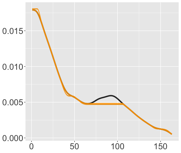
Figure 5: Estimated background monotone component on the Coronavirus dataset: the black curve represents the fitted density; the center orange curve represents the computed $\hat{h}_{0}$; and the top and bottom orange curves represent the 95% simultaneous confidence bands for $h_{0}$. (Due to the large amount of data here the confidence bands are very narrow.)

4 Log-concave background component

Our last emblematic setting is that of extracting a log-concave background component from a density. Log-concave densities have been widely studied in the literature (Walther, 2009; Samworth, 2018), and include a wide variety of distributions, including all Gaussian densities, all Laplace densities, all exponential densities, and all uniform densities. They have been extensively used in mixture models (Chang and Walther, 2007; Hu et al., 2016; Pu and Arias-Castro, 2020).

Following Patra and Sen (2016), for a density $f$ we define

$$\pi_{0}:=\sup\big{\{}\pi:\exists g\in\mathcal{C}\text{ s.t. }f-\pi g\geq 0\text{ a.e.}\big{\}},$$ (24)

where $\mathcal{C}$ is the class of log-concave densities. Note that $\pi_{0}\in[0,1]$, with $\pi_{0}=1$ if and only if $f$ itself is log-concave.

Theorem 7.

$\pi_{0}$ is the value of following optimization problem:

maximize $$\quad\int_{-\infty}^{\infty}h(x)dx$$ (25)

over $$\quad\big{\{}h:\mathbb{R}\xrightarrow{}\mathbb{R}_{+},\ \text{log-concave},\ h\leq f\big{\}}.$$

Indeed, this problem admits a solution, although it may not be unique.

Proof.

From the definition in (24), it is clear that

$$\pi_{0}=\sup\big{\{}\textstyle{\int h}:\text{$h$ is log-concave and $0\leq h\leq f$ a.e.}\big{\}}.$$ (26)

Thus we only need to show that the problem (25) admits a solution — and then show that it may not be unique to complete the proof. Here the arguments are a bit more involved.

Let $(h_{k})$ be a solution sequence to the problem (25), meaning that $h_{k}:\mathbb{R}\to\mathbb{R}_{+}$ is log-concave and satisfies $h_{k}\leq f$, and that $q_{k}:=\int h_{k}$ converges, as $k\to\infty$, to the value of the optimization problem (25), denoted $q_{*}$ henceforth. Note that $0\leq q_{k}\leq 1$ since $0\leq h_{k}\leq f$ and $\int f=1$, implying that $0\leq q_{*}\leq 1$. We only need to consider the case where $q_{*}>0$, for when $q_{*}=0$ the constant function $h\equiv 0$ is a solution. Without loss of generality, we assume that $q_{k}>0$ for all $k$.

Each $h_{k}$ is log-concave, and from this we know the following: its support is an interval, which we denote $[a_{k},b_{k}]$ with $-\infty\leq a_{k}<b_{k}\leq\infty$; $h_{k}$ is continuous and strictly positive on $(a_{k},b_{k})$; and $x\mapsto(\log h_{k}(y)-\log h_{k}(x))/(y-x)$ is non-increasing in $x\leq y$ and $y\mapsto(\log h_{k}(y)-\log h_{k}(x))/(y-x)$ is non-increasing in $y\geq x$. Extracting a subsequence if needed, we assume without loss of generality that $a_{k}\to a$ and $b_{k}\to b$ as $k\to\infty$, for some $-\infty\leq a\leq b\leq\infty$.

Define $F(t)=\int_{-\infty}^{t}f(x)dx$ and $H_{k}(t)=\int_{-\infty}^{t}h_{k}(x)dx$. We have that $H_{k}$ is a non-decreasing, and if $s\leq t$, $H_{k}(t)-H_{k}(s)\leq F(t)-F(s)$, because $h_{k}\leq f$. In particular, by Helly’s selection theorem (equivalent to Prokhorov’s theorem when dealing with distribution functions), we can extract a subsequence that converges pointwise. Without loss of generality, we assume that $(H_{k})$ itself converges, and let $H$ denote its limit. Note that $H$ is constant outside of $[a,b]$. In fact, $H(x)=0$ when $x<a$, because $x<a_{k}$ eventually, forcing $H_{k}(x)=0$. For $x,x^{\prime}>b$, we have that $x,x^{\prime}>b_{k}$ for large enough $k$, implying that $H_{k}(x)=H_{k}(x^{\prime})$, yielding $H(x)=H(x^{\prime})$ by taking the limit $k\to\infty$. Note also that, for all $s\leq t$,

$$H(t)-H(s)=\lim_{k\to\infty}(H_{k}(t)-H_{k}(s))\leq F(t)-F(s).$$

This implies that $H$ is absolutely continuous with derivative, denoted $h$, satisfying $h\leq f$ a.e..

We claim that $h$ is a solution to (25). We already know that $0\leq h\leq f$ a.e.. In addition, we also have $\int_{-\infty}^{\infty}h\geq q_{*}$. To see this, fix $\varepsilon>0$, and let $t$ be large enough that $\int_{t}^{\infty}f\leq\varepsilon$. Because $h_{k}\leq f$, we have $H_{k}(t)=q_{k}-\int_{t}^{\infty}h_{k}\geq q_{k}-\varepsilon$, implying that $H(t)\geq q_{*}-\varepsilon$ by taking the limit as $k\to\infty$. Hence, $\int_{-\infty}^{\infty}h=H(\infty)\geq H(t)\geq q^{*}-\varepsilon$, and $\varepsilon>0$ being otherwise arbitrary, we deduce that $\int_{-\infty}^{\infty}h\geq q_{*}$. It thus remains to show that $h$ is log-concave.

We establish this claim by proving that, extracting a subsequence if needed, $h_{k}$ converges to $h$ a.e., and it is enough to do so in an interval. Thus let $x_{0}$ and $\Delta>0$ be such that $[x_{0}-4\Delta,x_{0}+4\Delta]\subset(a,b)$. Note that $H$ is strictly increasing on $(a,b)$, because each $H_{k}$ is strictly increasing on $(a_{k},b_{k})$ due to $h_{k}$ being log-concave. Take any $x_{0}-\Delta\leq x<y\leq x_{0}+\Delta$ and let $\delta_{k}=(\log h_{k}(y)-\log h_{k}(x))/(y-x)$. We assume, for example, that $\delta_{k}\geq 0$, and bound it from above. Let $z_{k}\in[x_{0}-4\Delta,x_{0}-3\Delta]$ be such that $H_{k}(x_{0}-3\Delta)-H_{k}(x_{0}-4\Delta)=h_{k}(z_{k})\Delta$, which exists by the mean-value theorem. Note that $h_{k}(z_{k})\Delta\to\Delta_{1}:=H(x_{0}-3\Delta)-H(x_{0}-4\Delta)$, so that $h_{k}(z_{k})\geq\Delta_{2}:=\Delta_{1}/2\Delta>0$, eventually. Now, for any $z$ in $[x_{0}-2\Delta,x_{0}-\Delta]$, due to $z_{k}<z<x<y$ and $\log h_{k}$ being concave,

$$\frac{\log h_{k}(z)-\log h_{k}(z_{k})}{z-z_{k}}\geq\frac{\log h_{k}(y)-\log h_{k}(x)}{y-x}=\delta_{k},$$

which implies

$$h_{k}(z)\geq h_{k}(z_{k})\exp(\delta_{k}(z-z_{k}))\geq\Delta_{2}\exp(\delta_{k}\Delta).$$

This being true for all such $z$, we have

$$1\geq\int_{-\infty}^{\infty}f(z){\rm d}z\geq\int_{-\infty}^{\infty}h_{k}(z){\rm d}z\geq\int_{x_{0}-2\Delta}^{x_{0}-\Delta}h_{k}(z){\rm d}z\geq\Delta\cdot\Delta_{2}\exp(\delta_{k}\Delta),$$

allowing us to derive $\delta_{k}\leq M_{1}:=\Delta^{-1}\log(2/\Delta_{1})$. We can deal with the case where $\delta_{k}<0$ by symmetry, obtaining that, for all $k$ sufficiently large and all $x_{0}-\Delta\leq x<y\leq x_{0}+\Delta$,

$$\left|\frac{\log h_{k}(y)-\log h_{k}(x)}{y-x}\right|\leq M_{1}.$$

Let $u_{k}=h_{k}(x_{0})$. Because $h_{k}$ is unimodal, either $h_{k}(x)\leq u_{k}$ for all $x\leq x_{0}$ or $h_{k}(x)\leq u_{k}$ for all $x\geq x_{0}$. Extracting a subsequence if needed, and by symmetry, assume that the former is true for all $k$ large enough. Then

$$\Delta_{1} =H(x_{0}-3\Delta)-H(x_{0}-4\Delta)$$

$$=\lim_{k\to\infty}(H_{k}(x_{0}-3\Delta)-H_{k}(x_{0}-4\Delta))$$

$$=\lim_{k\to\infty}\int_{x_{0}-3\Delta}^{x_{0}-4\Delta}h_{k}(x){\rm d}x$$

$$\leq\liminf_{k\to\infty}\Delta u_{k},$$

so that $u_{k}\geq\Delta_{2}>0$, eventually. Assuming so, we have $u_{k}h_{k}(x_{0})\geq\Delta_{1}/\Delta\geq\Delta_{2}$. And we also have $h_{k}(x_{0})\leq f(x_{0})$, and together, $|\log h_{k}(x_{0})|\leq M_{2}:=|\log(\Delta_{2})|\vee|\log f(x_{0})|$. With the triangle inequality, we thus have, for all $x\in[x_{0}-\Delta,x_{0}+\Delta]$,

$$|\log h_{k}(x)|\leq M_{1}|x-x_{0}|+|\log h_{k}(x_{0})|\leq M_{1}\Delta+M_{2}=:M_{3}.$$

The family of functions $(\log h_{k})$ (starting at $k$ large enough) is thus uniformly bounded and equicontinuous on $[x_{0}-\Delta,x_{0}+\Delta]$, so that by the Arzelà–Ascoli theorem, we have that $(\log h_{k})$ is precompact for the uniform convergence on that interval. Therefore, the same is true for $(h_{k})$. Let $h_{\infty}$ be the uniform limit of a subsequence, and note that $h_{\infty}$ is continuous. $h_{\infty}$ must also be a weak limit as well, since uniform convergence on a compact interval implies weak convergence on that interval. Therefore $h_{\infty}=h$ a.e. on that interval, since $(h_{k})$ converges weakly to $h$. Hence, all the uniform limits of $(h_{k})$ must coincide with $h$ a.e., and since any such limit must be continuous, it means that they are the same. We conclude that, on the interval under consideration, $h$ is equal a.e. to a continuous function which is the (only) uniform limit of $(h_{k})$, and in particular, $(h_{k})$ converges pointwise a.e. to $h$ on that interval.

Thus, we have proved that the optimization problem (25) has at least one solution. We now show that there may be multiple solutions. This is the case, for instance, when $f=\frac{1}{m}f_{1}+\cdots+\frac{1}{m}f_{m}$ where each $f_{j}$ is a log-concave density and these densities have support sets that are pairwise disjoint. In that case, any of the components, meaning any $f_{j}$, is a solution to (25), and these are the only solutions. This comes from the fact that the support of a log-concave distribution is necessarily an interval. ∎

We have thus established that a density has at least one log-concave background component, and possibly multiple ones, corresponding to the solutions to (25). If $h$ is one such solution, then $\pi_{0}=\int h$ and we may define the corresponding density as $g=h/\pi_{0}$ if $\pi_{0}>0$. Then $f$ can be expressed as a mixture of the background density $g$ and another, unspecified, density $u$, as follows

$$f=\pi_{0}g+(1-\pi_{0})u.$$ (27)

(We do not use the notation $h_{0}$ and $g_{0}$ here, since these may not be uniquely defined.) The procedure is summarized in Table 11. An illustration of this decomposition is shown in Figure 6. Note that the density $u$ may have a non-trivial log-concave background component. This is the case, for example, if $f$ is the (nontrivial) mixture of two log-concave densities with disjoint support sets, in which case $u$ is one of these log-concave densities.

Table 11: Log-concave background computation. (The input $d$ is used to initialize the function $v$ — discretized as $\mathbf{v}$ below — that is bounded from above by $\log f$. In our experiments, we chose $d=0.02$.)

inputs: equally spaced gridpoints $\mathbf{t}=\{t_{1},t_{2},\dots,t_{k}\}$, density $f$, a boolean $R$ indicating whether to use the Riemann integral approximation, initialization amount $d$
initialize $\mathbf{w}=(0,0,\dots,0)$ with length $k$ for $i=1,\dots,k$ do $\mathbf{w}[i]=\log(f(t_{i}))$ compute $\mathbf{A}$ and $\mathbf{b}$ as in (36) initialize $\mathbf{v}=\mathbf{w}-(d,d,\dots,d)$ if $R$ = true then do optimization (44) using SQP, and record the optimizer $\mathbf{v}$ and the maximum as $\pi_{0}$ else do optimization (33) using SQP, and record the optimizer $\mathbf{v}$ and the maximum as $\pi_{0}$
return $\mathbf{v},\pi_{0}$

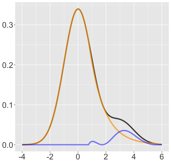
Figure 6: The density $f$ of the Gaussian mixture $0.85\text{ }\mathcal{N}(0,1)+0.15\text{ }\mathcal{N}(3,1)$, in black, and its decomposition into $\pi_{0}g$, in orange, and $(1-\pi_{0})u$, in blue. The orange curve is acquired by maximizing (34), but maximizing the Riemann integral approximation (44) gives almost the same result (with the maximum difference between the two curves being $2\times 10^{-14}$). Notice $\pi_{0}=0.931$ as $\pi_{0}g$ also takes a non-negligible weight from the smaller component $0.15\text{ }\mathcal{N}(0,1)$.

4.1 Estimation and consistency

In practice, based on a sample, we estimate $f$, resulting in $\hat{f}$, and simply obtain estimates by plug-in as we did before, this time via

maximize $$\quad\int_{-\infty}^{\infty}h(x)dx$$ (28)

over $$\quad\big{\{}h:\mathbb{R}\xrightarrow{}\mathbb{R}_{+},\ \text{log-concave},\ h\leq\hat{f}\big{\}}.$$

At least formally, let $\hat{h}$ be a solution to (28). We then define

$$\hat{\pi}_{0}=\int_{-\infty}^{\infty}\hat{h}(x)dx, \hat{g}(x)=\frac{\hat{h}(x)}{\hat{\pi}_{0}}.$$ (29)

Here, to avoid technicalities, we work under the assumption that the density estimator $\hat{f}=\hat{f}_{n}$ satisfies

$$\operatorname{\mathbb{E}}\left[\operatorname*{ess\,sup}_{|x|\leq a}\frac{\max\{\hat{f}_{n}(x),f(x)\}}{\min\{\hat{f}_{n}(x),f(x)\}}\right]\to 1,\quad n\to\infty,\quad\forall a>0.$$ (30)

This condition is better suited for when the density $f$ approaches 0 only at infinity. Also for the sake of simplicity, we only establish consistency for $\hat{\pi}_{0}$.

Theorem 8.

When (30) holds, $\hat{\pi}_{0}$ is a consistent.

Proof.

Fix $\eta>0$ and $a>0$, and consider the event, denoted $\Omega$, that

$$\operatorname*{ess\,sup}_{|x|\leq a}\frac{\max\{\hat{f}(x),f(x)\}}{\min\{\hat{f}(x),f(x)\}}\leq 1+\eta.$$ (31)

Because of (30), $\Omega$ happens with probability tending to 1 as the sample size increases. Let $\varepsilon=1-\int_{[-a,a]}f$, which is small when $a$ is large.

Assume that $\Omega$ holds. Let $h$ be a solution to (25), so that $\pi_{0}=\int h$. Then define $\tilde{h}(x)=(1-\eta)h(x)\mathds{1}\{|x|\leq a\}$ and note that

$$\int\tilde{h}=(1-\eta)\int_{[-a,a]}h\geq(1-\eta)(\pi_{0}-\varepsilon),$$

so that $\int\tilde{h}$ is close to $\pi_{0}$ when $\eta$ is small and $a$ is large. We also note that $\tilde{h}$ is log-concave and satisfies $0\leq\tilde{h}\leq(1-\eta)f$ a.e.. Under $\Omega$, we have $f\leq(1+\eta)\hat{f}$, and so it is also the case that $\tilde{h}\leq(1-\eta)(1+\varepsilon)\hat{f}\leq\hat{f}$, assuming as we do that $\eta$ and $\varepsilon$ are small enough. Then $\int\tilde{h}\leq\hat{\pi}_{0}$, by definition of $\hat{\pi}_{0}$. Gathering everything, we obtain that $(1-\eta)(\pi_{0}-\varepsilon)\leq\hat{\pi}_{0}$. By letting $\eta\to 0$ and $a\to\infty$ so that $\varepsilon\to 0$, we have established that $\liminf\hat{\pi}_{0}\geq\pi_{0}$ in probability. (The $\liminf$ needs to be understood as the sample size increases.)

The reverse relation, meaning $\limsup\hat{\pi}_{0}\leq\pi_{0}$, can be derived similarly starting with a solution $\hat{h}$ to (28). ∎

Confidence interval

Once again, if we have available a confidence band for $f$, we can deduce from that a confidence interval for $\pi_{0}$.

Theorem 9.

Suppose that we have a confidence band for $f$ as in (11). Then

$$\hat{\pi}_{l}\leq\pi_{0}\leq\hat{\pi}_{u}$$ (32)

holds with probability at least $1-\alpha$, where $\hat{\pi}_{l}$ and $\hat{\pi}_{u}$ are the values of the optimization problem (25) with $f$ replaced by $\hat{f}_{l}$ and $\hat{f}_{u}$, respectively.

The proof is straightforward and thus omitted.

4.2 Numerical method

Unlike the previous sections, here the computation of our estimator(s) is non-trivial: indeed, after computing $\hat{f}$ with an off-the-shelf procedure, we need to solve the optimization problem (28). Thus, in this section, we discuss how to solve this optimization problem.

Although least concave majorants (or equivalently greatest convex minorants) have been considered extensively in the literature, for example in (Franců et al., 2017; Jongbloed, 1998), the problem (25) calls for a type of greatest concave minorant, and we were not able to find references in the literature that directly tackle this problem. We do want to mention (Gorokhovik, 2019), where a similar concept is discussed, but the definition is different from ours and no numerical procedure to solve the problem is provided. For lack of structure to exploit, we propose a direct discretization followed by an application of sequential quadratic programming (SQP), first proposed by Wilson (1963). For more details on SQP, we point the reader to (Gill and Wong, 2012) or (Nocedal and Wright, 2006, Ch 18).

Going back to (25), where here $f$ plays the role of a generic density on the real line, the main idea is to restrict $v:=\log h$ to be a continuous, concave, piecewise linear function. Once discretized, the integral admits a simple closed-form expression and the concavity constraint is transformed into a set of linear inequality constraints.

To setup the discretization, for $k\geq 1$ integer, let $t_{-k,k}<t_{-k+1,k}<\cdots<t_{k-1,k}<t_{k,k}$ be such that $t_{j,k}=-t_{-j,k}$ (symmetry) and $t_{j+1,k}-t_{j,k}=\delta_{k}$ (equispaced) for all $j$, with $\delta_{k}\to 0$ (dense) and $t_{k,k}\to\infty$ as $k\to\infty$ (spanning the real line). Suppose that $v$ is concave with $v\leq\log f$ and to that function associate the triangular sequence $v_{j,k}:=v(t_{j,k})$. Then, for each $k$,

$$-v_{j+1,k}+2v_{j,k}-v_{j-1,k} =-v(t_{j+1,k})+2v(t_{j,k})-v(t_{j-1,k})$$

$$=2\big{(}v(t_{j,k})-\tfrac{1}{2}v(t_{j+1,k}+\delta_{k})-\tfrac{1}{2}v(t_{j-1,k}+\delta_{k})\big{)}\geq 0,\quad\text{for all }k,$$

by the fact that $v$ is concave. In addition, $v_{j,k}=v(t_{j,k})\leq\log f(t_{j,k})=:u_{j,k}$ (which are given). Instead of working directly with a generic concave function $v$, we work with those that are piecewise linear as they are uniquely determined by their values at the grid points if we further restrict them to be $=-\infty$ on $(-\infty,t_{-k,k})\cup(t_{k,k},+\infty)$. Effectively, at $k$, we replace in (25) the class $\mathcal{C}$ with the class $\mathcal{C}_{k}$ of functions $h$ such that $v=\log h$ is log-concave, linear on each interval $[t_{j,k},t_{j+1,k}]$, $v(x)=-\infty$ for $x<t_{-k,k}$ or $x>t_{k,k}$, and that satisfies $v(t_{j,k})\leq\log f(t_{j,k})$, for all $j$.

This leads us to the following optimization problem, which instead of being over a function space is over a Euclidean space:

$$\begin{split}\text{maximize}\quad&\Lambda(\mathbf{v})\\ \text{over}\quad&\mathbf{v}=[v_{-k,k},\dots,v_{k,k}]^{\top}\quad\text{such that}\quad\mathbf{A}\mathbf{v}\geq\mathbf{b},\end{split}$$ (33)

where

$$\Lambda(v_{-k},\dots,v_{k}):=\delta_{k}\sum_{j=-k}^{k-1}\lambda(v_{j},v_{j+1}),$$ (34)

$$\lambda(x,y):=\mathds{1}\{x\neq y\}\frac{\exp(x)-\exp(y)}{x-y}+\mathds{1}\{x=y\}\exp(x),$$ (35)

and where

$$\mathbf{A}=\begin{bmatrix}-1&2&-1&0&\dots&0&0&0\\ 0&-1&2&-1&\dots&0&0&0\\ \vdots&\vdots&\vdots&\vdots&\vdots&\vdots&\vdots&\vdots\\ 0&0&0&0&\dots&-1&2&-1\\ -1&0&0&0&\dots&0&0&0\\ 0&-1&0&0&\dots&0&0&0\\ \vdots&\vdots&\vdots&\vdots&\vdots&\vdots&\vdots&\vdots\\ 0&0&0&0&\dots&0&0&-1\end{bmatrix},\qquad\mathbf{b}=\begin{bmatrix}0\\ 0\\ \vdots\\ 0\\ -u_{1}\\ -u_{2}\\ \vdots\\ -u_{k}\end{bmatrix}\,.$$ (36)

As we are not aware of any method that could solve (33) exactly, we will use sequential quadratic programming (SQP). In our implementation we use the R package nloptr  based on an original implementation of Kraft (1988).

Theorem 10.

Assume that $f$ is Lipschitz and locally bounded away from 0. Then the value of discretized optimization problem (33) converges, as $k\to\infty$, to the value of the original optimization problem (25).

The assumptions made on $f$ are really for convenience — to expedite the proof of the result while still including interesting situations — and we do expect that the result holds more broadly. We also note that, in our workflow, the problem (33) is solved for $\hat{f}$, and that $\hat{f}$ satisfies these conditions (remember that the sample size is held fixed here) if it is a kernel density estimator based on a smooth kernel function supported on the entire real line like the Gaussian kernel.

Proof.

Let $h$ be a solution to (25) so that $\int h=\pi_{0}$, where $\pi_{0}$ denotes the value of (25). Define $v=\log h$ and let $v_{j,k}=v(t_{j,k})$. As we explained above, this makes $\mathbf{v}_{k}:=(v_{-k,k},\dots,v_{k,k})$ feasible for (33). Therefore $\Lambda(\mathbf{v}_{k})\leq\pi_{0,k}$, where $\pi_{0,k}$ denotes the value of (33). On the other hand, let $\tilde{v}_{k}$ denote the piecewise linear approximation to $v$ on the grid, meaning that $\tilde{v}_{k}(x)=-\infty$ if $x<t_{-k,k}$ or $x>t_{k,k}$, $\tilde{v}_{k}(t_{j,k})=v(t_{j,k})$ and $\tilde{v}_{k}$ linear on $[t_{j,k},t_{j+1,k}]$ for all $j$. We then have

$$\Lambda(\mathbf{v}_{k})=\int\tilde{h}_{k}\xrightarrow{k\to\infty}\int h,$$ (37)

where the convergence is justified, for example, by the fact that $\tilde{h}_{k}\to h$ pointwise and $0\leq\tilde{h}_{k}\leq h$ (because, by concavity of $v$, $v\geq\tilde{v}_{k}$), so that the dominated convergence theorem applies. From this we get that

$$\liminf_{k\to\infty}\pi_{0,k}\geq\pi_{0}.$$ (38)

In the other direction, let $\mathbf{v}_{k}$ be a solution of (33), so that $\Lambda(\mathbf{v}_{k})=\pi_{0,k}$. Let $\tilde{v}_{k}$ denote the linear interpolation of $\mathbf{v}_{k}$ on the grid $(t_{-k,k},\dots,t_{k,k})$, defined exactly as done above, and let $\tilde{h}_{k}=\exp(\tilde{v}_{k})$. We have that $\tilde{h}_{k}\leq f$ at the grid points, but not necessarily elsewhere. To work in that direction, fix $a>0$, taken arbitrarily large in what follows. Because of our assumptions on $f$, we have that $u:=\log f$ is Lipschitz on $[-a,a]$, say with Lipschitz constant $L$. In particular, with $\tilde{u}_{k}$ denoting the linear approximation of $u$ based on the grid, we have

$$|u(x)-\tilde{u}_{k}(x)|\leq L\delta_{k}=:\eta_{k}.$$ (39)

Define $\bar{v}_{k}(x)=\tilde{v}_{k}(x)-\eta_{k}$ if $x\in[-a,a]$ and $\bar{v}_{k}(x)=-\infty$ otherwise. Note that $\bar{v}_{k}$ is also concave and piecewise linear, and because $\tilde{h}_{k}\leq f$, $\tilde{v}_{k}\leq\tilde{u}_{k}$, we have

$$\bar{v}_{k}(x)=\tilde{v}_{k}(x)-\eta_{k}\leq\tilde{u}_{k}(x)-\eta_{k}\leq u(x),\quad\forall x\in[-a,a].$$ (40)

In particular, $\bar{h}_{k}:=\exp(\bar{v}_{k})$ is feasible for (25), implying that $\int\bar{h}_{k}\leq\pi_{0}$. On the other hand, we have

$$\int\bar{h}_{k}=\int\exp(\bar{v}_{k})=\exp(-\eta_{k})\int_{[-a,a]}\exp(\tilde{v}_{k})=\exp(-\eta_{k})\int_{[-a,a]}\tilde{h}_{k},$$ (41)

and so, because $\tilde{h}_{k}\leq\tilde{f}_{k}:=\exp(\tilde{u}_{k})$,

$$\pi_{0,k}=\Lambda(\mathbf{v}_{k})=\int\tilde{h}_{k} =\int_{[-a,a]}\tilde{h}_{k}+\int_{[-a,a]^{\mathsf{c}}}\tilde{h}_{k}$$

$$=\exp(\eta_{k})\int\bar{h}_{k}+\int_{[-a,a]^{\mathsf{c}}}\tilde{h}_{k}$$

$$\leq\exp(\eta_{k})\pi_{0}+\int_{[-a,a]^{\mathsf{c}}}\tilde{f}_{k}.$$

Given $\varepsilon>0$ arbitrarily small, choose $a$ large enough that $\int_{[-a,a]^{\mathsf{c}}}f\leq\varepsilon$. Since

$$\int_{[-a,a]^{\mathsf{c}}}\tilde{f}_{k}\xrightarrow{k\to\infty}\int_{[-a,a]^{\mathsf{c}}}f,$$ (42)

for $k$ large enough we have $\int_{[-a,a]^{\mathsf{c}}}\tilde{f}_{k}\leq 2\varepsilon$, implying that $\pi_{0,k}\leq\exp(\eta_{k})\pi_{0}+2\varepsilon$. Using the fact that $\exp(\eta_{k})\to 1$ since $\eta_{k}=L\delta_{k}\to 0$, and that $\varepsilon>0$ is arbitrary, we get that

$$\limsup_{k\to\infty}\pi_{0,k}\leq\pi_{0},$$ (43)

concluding the proof. ∎

We mention that besides the discretization (33), we also considered a more straightforward discretization of the integral, effectively replacing $\Lambda$ in (33) with $\Lambda_{0}$ defined as

$$\Lambda_{0}(v_{-k},\dots,v_{k}):=\delta_{k}\left(\tfrac{1}{2}\exp(v_{-k})+\tfrac{1}{2}\exp(v_{k})+\sum_{j=-k+1}^{k-1}\exp(v_{j})\right).$$ (44)

The outputs returned by these two discretizations, (33) and (44), were very similar in our numerical experiments.

4.3 Numerical experiments

In this subsection we consider experiments where the background component could be assumed to be log-concave. The density fitting process and confidence band acquisition are exactly the same as in Section 2.2. We first consider four different situations as listed in Table 12. Although the mixture distributions are identical to those in Table 3 for the symmetric case, we need to point out that $\pi_{0}$ is different here, as $\pi_{0}$ here corresponds to the largest possible log-concave component as defined in (24). We again generate a sample of size $n=1000$ from each model, and repeat each setting $1000$ times.

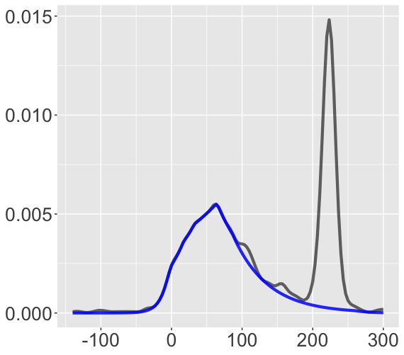
(a) Carina dataset

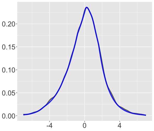
(b) Leukemia dataset

Figure 10: Carina (radial velocity) and Leukemia ($z$ values) datasets with kernel density, with bandwidth chosen ‘by hand’ instead of by cross-validation: the black curve represents fitted density with increased bandwidth; the blue curve represents the computed $\hat{h}$. We note that for the Carina dataset, the bandwidth was increased from $3.085$ to $6$, and $\hat{\pi}_{0}$ changed from $0.550$ to $0.600$. For the Leukemia dataset, the bandwidth was been increased from $0.124$ to $0.25$, and $\hat{\pi}_{0}$ changed from $0.939$ to $0.981$.

We note that the output of our algorithm depends heavily on the estimation of the density $\hat{f}$. When the bandwidth selected by cross-validation yields a density with a high frequency of oscillation, the largest log-concave component is very likely to be smaller than the correct value. For an illustrative situation, see Figure 7. In the event that such a situation happen, we recommend that the user look at a plot of $\hat{f}$ before applying our procedure, with the possibility of selecting a larger bandwidth. This is what we did, for example, for the Carina and Leukemia datasets in Figure 10. In the simulations, to avoid the effect of these issue, we report the median value instead of the mean. These values are reported in Table 13.

As can be seen, even with only the assumption of log-concavity, our method is accurate in estimating $\pi_{0}$, with estimation errors ranging from $0.001$ to $0.007$. Our method frequently achieves smaller error in estimating $\pi_{0}$ than comparison methods in estimating $\theta_{0}$ and $\theta$, and does so with less information on the background component. For situations where the background component is specified incorrectly, we invite the reader to Section 5.1.

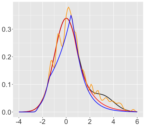
Figure 7: An illustrative situation that occurred in the course of our simulations, where a high frequency of oscillation of $\hat{f}$ results in a significantly lower estimation for $\pi_{0}$: a Gaussian mixture density $0.85\text{ }\mathcal{N}(0,1)+0.15\text{ }\mathcal{N}(0,1)$, in black, and corresponding largest log-concave component $h$, in red, with the fitted density $\hat{f}$, in orange, and fitted largest log-concave component $\hat{h}$, in blue. Here, as before, $\hat{f}$ is obtained by kernel density estimation with bandwidth chosen by cross-validation. The result based on this estimate is $\hat{\pi}_{0}=0.807$, while the actual value is $\pi_{0}=0.931$.

Remark 3.

We note that here the SQP algorithm as implemented in the R package nloptr sometimes gives $\hat{h}=0$ as the largest log-concave component due to some parts of the estimated density $\hat{f}$ being $0$. This situation happens occasionally when computing the lower confidence bound, and it is of course incorrect in situations like those in Table 12. When this situation occurs, we rerun the algorithm on the largest interval of non-zero $\hat{f}$ values and report the greatest log-concave component acquired on that interval.

Table 12: Log-concave simulation situations of Gaussian mixtures, as well as values of $\theta$, $\theta_{0}$, and $\pi_{0}$, obtained through numerical optimization.

Model	Distribution	$\theta$	$\theta_{0}$	$\pi_{0}$
L1	$0.85\text{ }\mathcal{N}(0,1)+0.15\text{ }\mathcal{N}(3,1)$	0.850	0.850	0.931
L2	$0.95\text{ }\mathcal{N}(0,1)+0.05\text{ }\mathcal{N}(3,1)$	0.950	0.950	0.981
L3	$0.85\text{ }\mathcal{N}(0,1)+0.1\text{ }\mathcal{N}(2.5,0.75)+0.05\text{ }\mathcal{N}(-2.5,0.75)$	0.850	0.851	0.975
L4	$0.85\text{ }\mathcal{N}(0,1)+0.1\text{ }\mathcal{N}(2.5,0.75)+0.05\text{ }\mathcal{N}(5,0.75)$	0.850	0.850	0.946

Table 13: A comparison of various methods for estimating a log-concave background component in the situations of Table 12. Here we report the median values instead of the mean values (and also report the standard deviations, as before). As always, $\hat{\pi}_{0}$ should be compared with $\pi_{0}$, $\hat{\theta}_{0}^{X}$ should be compared with $\theta_{0}$, and $\hat{\theta}^{X}$ should be compared with $\theta$.

Model	$\hat{\pi}_{0}$	$\hat{\pi}_{0}^{\rm{L}}$	$\hat{\pi}_{0}^{\rm{U}}$	Null	$\hat{\theta}_{0}^{\rm{PSC}}$	$\hat{\theta}_{0}^{\rm{PSH}}$	$\hat{\theta}_{0}^{\rm{PSB}}$	$\hat{\theta}^{\rm{E}}$	$\hat{\theta}^{\rm{MR}}$	$\hat{\theta}^{\rm{CJ}}$
L1	0.932	0.596	1	$\mathcal{N}(0,1)$	0.850	0.858	0.894	0.861	0.890	0.888
	(0.034)	(0.074)	(0)		(0.024)	(0.023)	(0.018)	(0.023)	(0.014)	(0.085)
L2	0.974	0.662	1	$\mathcal{N}(0,1)$	0.942	0.958	0.988	0.953	0.972	0.964
	(0.028)	(0.080)	(0)		(0.023)	(0.022)	(0.015)	(0.026)	(0.008)	(0.082)
L3	0.969	0.611	1	$\mathcal{N}(0,1)$	0.864	0.948	0.936	0.856	0.896	0.705
	(0.031)	(0.077)	(0)		(0.023)	(0.034)	(0.017)	(0.024)	(0.015)	(0.085)
L4	0.942	0.632	1	$\mathcal{N}(0,1)$	0.848	0.857	0.893	0.849	0.890	0.712
	(0.033)	(0.074)	(0)		(0.023)	(0.024)	(0.018)	(0.024)	(0.014)	(0.088)

4.4 Real data analysis

In this subsection we examine real datasets of two component mixtures where the background component could be assumed to be log-concave. We first consider the six real datasets presented in Section 2.3, but this time look for a background log-concave component. When the background is known, the numerical results of the Prostate and Carina datasets can be found in Table 14, Figure 8(a) and Figure 8(b). When the background is unknown, the numerical results of the HIV, Leukemia, Parkinson and Police datasets can be found in Table 15, Figure 9(a), Figure 9(b), Figure 9(c) and Figure 9(d).

In addition to the above six datasets, we also include here the Old Faithful Geyser dataset (Azzalini and Bowman, 1990). This dataset consists of $272$ waiting times, in minutes, between eruptions for the Old Faithful Geyser in Yellowstone National Park, Wyoming, USA. We attempt to find the largest log-concave component of the waiting times. The results are summarized in the first row of Table 15, Figure 11(a) and Figure 11(b). We want to note from this example that the curve $\hat{h}_{u}$ acquired from $\hat{f}_{u}$ leading to the computation of $\hat{\pi}_{0}^{\rm U}$, is not the upper confidence bound of $h_{0}$, as shown by Figure 11(a).

Remark 4.

We observe here through these real datasets that compared to symmetric background assumptions in Section 2.3, the largest log-concave background component usually has a higher weight than the largest symmetric background component.

Table 14: Real datasets where the background log-concave component is known. (Note that we work with $z$ values here instead of $p$-values so our result in Prostate dataset is slightly different from that in (Patra and Sen, 2016).)

Model	$\hat{\pi}_{0}$	$\hat{\pi}_{0}^{\rm{L}}$	$\hat{\pi}_{0}^{\rm{U}}$	Null	$\hat{\theta}_{0}^{\rm{PSC}}$	$\hat{\theta}_{0}^{\rm{PSH}}$	$\hat{\theta}_{0}^{\rm{PSB}}$	$\hat{\theta}^{\rm{E}}$	$\hat{\theta}^{\rm{MR}}$	$\hat{\theta}^{\rm{CJ}}$
Prostate	0.994	0.809	1	$\mathcal{N}(0,1)$	0.931	0.941	0.975	0.931	0.956	0.867
Carina	0.600	0.242	1	bgstars	0.636	0.645	0.677	0.951	0.664	0.206

Table 15: Real datasets where the background log-concave distribution is unknown. (Note that Efron’s method will not run on the Geyser dataset.)

Model	$\hat{\pi}_{0}$	$\hat{\pi}_{0}^{\rm{L}}$	$\hat{\pi}_{0}^{\rm{U}}$	$\hat{\theta}^{\rm{E}}$	$\hat{\theta}^{\rm{CJ}}$
Geyser	0.693	0.287	1	NA	1
HIV	0.984	0.804	1	0.940	0.926
Leukemia	0.981	0.695	1	0.911	0.820
Parkinson	1	0.605	1	0.998	0.993
Police	0.997	0.765	1	0.985	0.978

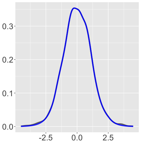
(a) Prostate dataset

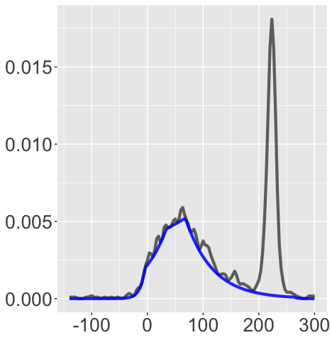
(b) Carina dataset

Figure 8: Estimated background log-concave component on the Prostate ($z$ values) and Carina (radial velocity) datasets: the black curve represents fitted density; the blue curve represents computed $\hat{h}$, one of the largest log-concave components. Due to unusually high frequency of oscillation in $\hat{f}$ in the Carina dataset, we consider increasing the bandwidth from the one acquired by cross-validation, and the corresponding result is shown in Figure 10(a).

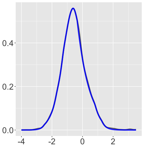
(a) HIV dataset

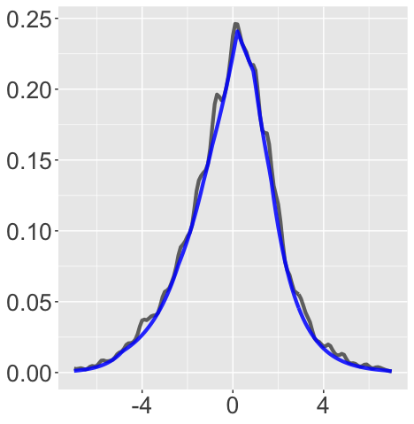
(b) Leukemia dataset

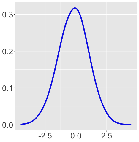
(c) Parkinson dataset

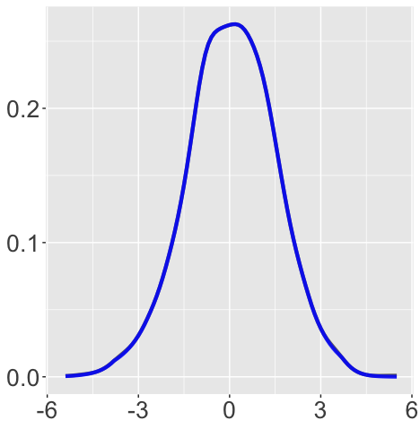
(d) Police dataset

Figure 9: Estimated background log-concave component on HIV ($z$ values), Leukemia ($z$ values), Parkinson ($z$ values), and Police ($z$ scores) datasets: the black curve represents fitted density; the blue curve represents computed $\hat{h}$, one of the largest log-concave components. Due to the high frequency of oscillation in $\hat{f}$ in the Leukemia dataset, we consider increasing the bandwidth from the one acquired by cross-validation, and the corresponding result is shown in Figure 10(b).

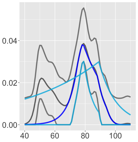
(a) Geyser dataset with $\hat{h}_{l}$ and $\hat{h}_{u}$

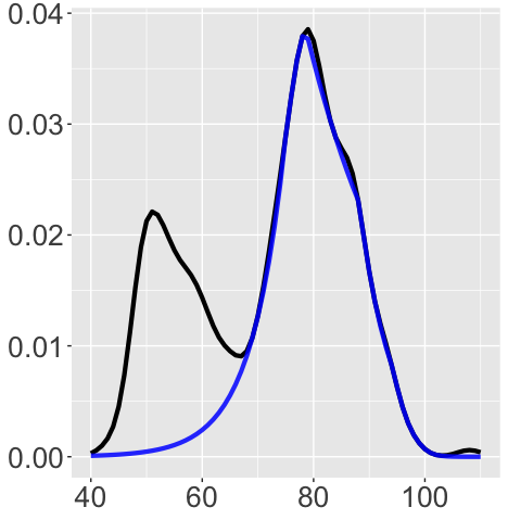
(b) Geyser dataset with only $\hat{h}$

Figure 11: Estimated background log-concave component on the Geyser (duration) dataset: the black curve represents the fitted density; the blue curve represents the computed $\hat{h}$; the gray curves (left) represent $\hat{f}_{l}$ and $\hat{f}_{u}$; the light blue curves (left) represents $\hat{h}_{l}$ and $\hat{h}_{u}$. Note from the left plot that $\hat{h}_{u}$ is only used to compute $\hat{\pi}_{0}^{\rm U}$, and is not an upper bound for $h$.

5 Conclusion and discussion

In this paper, we extend the approach of Patra and Sen (2016) to settings where the background component of interest is assumed to belong to three emblematic examples: symmetric, monotone, and log-concave. In each setting, we derive estimators for both the proportion and density for the background component, establish their consistency, and provide confidence intervals/bands. However, the important situation of incorrect background distribution and other extensions remain unaddressed, and therefore we discuss them in this section.

5.1 Incorrect background specification

As mentioned in Section 2.2 and Section 4.3, our method requires much less information than comparable methods, and therefore is much less prone to misspecification of the background component. In this subsection, we give an experiment illustrating this point. We consider the mixture model: $0.85\text{ }\mathcal{T}_{6}+0.15\text{ }\mathcal{N}(3,1).$ Instead of the correct null distribution $\mathcal{T}_{6}$, we take it to be $\mathcal{N}(0,1)$. This situation could happen in situations of multiple testing settings, for example in the HIV dataset in Section 2.3. We consider both a symmetric background and log-concave background on this model in Table 16, and report the fitted values of our method and comparison methods in Table 17. As can be seen, when estimating $\pi_{0}$, our estimator achieves $0.002$ error when assuming symmetric background and $0.004$ error when assuming log-concave background, less then any other method in comparison that estimates $\theta_{0}$ or $\theta$. The heuristic estimator of Patra and Sen (2016) has slightly higher error than our method, while the constant estimator of Patra and Sen (2016) and the estimators of Efron (2007) and Cai and Jin (2010) have large errors. The upper confidence bound of Meinshausen and Rice (2006) also becomes incorrect.

Table 16: Simulation situations when background specification is incorrect, as well as values of $\theta$, $\theta_{0}$, $\pi_{0}$, obtained through numerical optimization.

Model	Background	Distribution	$\theta$	$\theta_{0}$	$\pi_{0}$
S5	Symmetric	$0.85\text{ }\mathcal{T}_{6}+0.15\text{ }\mathcal{N}(3,1)$	0.850	0.850	0.859
L5	Log-concave	$0.85\text{ }\mathcal{T}_{6}+0.15\text{ }\mathcal{N}(3,1)$	0.850	0.850	0.925

Table 17: Results for the situations of Table 16. We provide mean values in S5, and median values in L5.

Model	Center	$\hat{\pi}_{0}$	$\hat{\pi}_{0}^{\rm{L}}$	$\hat{\pi}_{0}^{\rm{U}}$	Null	$\hat{\theta}_{0}^{\rm{PSC}}$	$\hat{\theta}_{0}^{\rm{PSH}}$	$\hat{\theta}_{0}^{\rm{PSB}}$	$\hat{\theta}^{\rm{E}}$	$\hat{\theta}^{\rm{MR}}$	$\hat{\theta}^{\rm{CJ}}$
S5	0.073	0.857	0.541	1	$\mathcal{N}(0,1)$	0.815	0.855	0.877	0.803	0.843	0.816
	(0.057)	(0.021)	(0.057)	(0)		(0.021)	(0.022)	(0.016)	(0.026)	(0.015)	(0.086)
L5		0.921	0.574	1	$\mathcal{N}(0,1)$	0.817	0.856	0.877	0.803	0.843	0.814
		(0.036)	(0.069)	(0)		(0.021)	(0.022)	(0.016)	(0.026)	(0.015)	(0.086)

5.2 Combinations

Although not discussed in the main part of the paper, some combinations of the shape constraints considered earlier are possible. For example, one could consider extracting a maximal background that is symmetric and log-concave; or one could consider extracting a maximal background that is monotone and log-concave. As it turns out, these two combinations are intimately related. Mixtures of symmetric log-concave distributions are considered, for example, in (Pu and Arias-Castro, 2020).

5.3 Generalization to higher dimensions

All our examples were on the real line, corresponding to real-valued observations, simply because the work was in large part motivated by multiple testing in which the sample stands for the test statistics. But the approach is more general. Indeed, consider a measurable space, and let $\mathcal{D}$ be a class of probability distributions on that space. Given a probability distribution $\mu$, we can quantify how much there is of $\mathcal{D}$ in $\mu$ by defining

$$\pi_{0}:=\sup\big{\{}\pi:\exists\nu\in\mathcal{D}\text{ s.t. }\mu\geq\pi\nu\big{\}}.$$ (45)

For concreteness, we give a simple example in an arbitrary dimension $d$ by generalizing the setting of a symmetric background component covered in Section 2. Although various generalizations are possible, we consider the class — also denoted $\mathcal{S}$ as in (3) — of spherically symmetric (i.e., radial) densities with respect to the Lebesgue measure on $\mathbb{R}^{d}$. It is easy to see that the background component proportion is given by

$$\pi_{0}=\int_{\mathbb{R}^{d}}h_{0}(x)dx, h_{0}(x):=\min\{f(y):\|y\|=\|x\|\},$$ (46)

and, if $\pi_{0}>0$, the background component density is given by $g_{0}:=h_{0}/\pi_{0}$.

Acknowledgments

We are grateful to Philip Gill for discussions regarding the discretization of the optimization problem (25).

References

- Arias-Castro and Chen (2017) Arias-Castro, E. and S. Chen (2017). Distribution-free multiple testing. Electronic Journal of Statistics 11(1), 1983–2001.
- Arias-Castro and Wang (2017) Arias-Castro, E. and M. Wang (2017). Distribution-free tests for sparse heterogeneous mixtures. TEST 26(1), 71–94.
- Arlot and Celisse (2010) Arlot, S. and A. Celisse (2010). A survey of cross-validation procedures for model selection. Statistics Surveys 4, 40–79.
- Azzalini and Bowman (1990) Azzalini, A. and A. W. Bowman (1990). A look at some data on the Old Faithful Geyser. Journal of the Royal Statistical Society: Series C 39(3), 357–365.
- Benjamini and Hochberg (1995) Benjamini, Y. and Y. Hochberg (1995). Controlling the false discovery rate: a practical and powerful approach to multiple testing. Journal of the Royal Statistical Society: Series B 57(1), 289–300.
- Benjamini and Hochberg (2000) Benjamini, Y. and Y. Hochberg (2000). On the adaptive control of the false discovery rate in multiple testing with independent statistics. Journal of Educational and Behavioral Statistics 25(1), 60–83.
- Bickel and Rosenblatt (1973) Bickel, P. J. and M. Rosenblatt (1973). On some global measures of the deviations of density function estimates. The Annals of Statistics 1(6), 1071–1095.
- Bordes et al. (2006) Bordes, L., S. Mottelet, and P. Vandekerkhove (2006). Semiparametric estimation of a two-component mixture model. The Annals of Statistics 34(3), 1204–1232.
- Cai and Jin (2010) Cai, T. T. and J. Jin (2010). Optimal rates of convergence for estimating the null density and proportion of nonnull effects in large-scale multiple testing. The Annals of Statistics 38(1), 100–145.
- Cattaneo et al. (2019) Cattaneo, M. D., M. Jansson, and X. Ma (2019). lpdensity: Local polynomial density estimation and inference. arXiv preprint arXiv:1906.06529.
- Cattaneo et al. (2020) Cattaneo, M. D., M. Jansson, and X. Ma (2020). Simple local polynomial density estimators. Journal of the American Statistical Association 115(531), 1449–1455.
- Chang and Walther (2007) Chang, G. T. and G. Walther (2007). Clustering with mixtures of log-concave distributions. Computational Statistics & Data Analysis 51(12), 6242–6251.
- Chen (2017) Chen, Y.-C. (2017). A tutorial on kernel density estimation and recent advances. Biostatistics & Epidemiology 1(1), 161–187.
- Cheng and Chen (2019) Cheng, G. and Y.-C. Chen (2019). Nonparametric inference via bootstrapping the debiased estimator. Electronic Journal of Statistics 13(1), 2194–2256.
- Chow et al. (1983) Chow, Y.-S., S. Geman, and L.-D. Wu (1983). Consistent cross-validated density estimation. The Annals of Statistics 11(1), 25–38.
- Cline and Hart (1991) Cline, D. B. H. and J. D. Hart (1991). Kernel estimation of densities with discontinuities or discontinuous derivatives. Statistics 22(1), 69–84.
- Cohen (1967) Cohen, A. C. (1967). Estimation in mixtures of two normal distributions. Technometrics 9(1), 15–28.
- Dong et al. (2021) Dong, E., H. Du, and L. Gardner (2021). An interactive web-based dashboard to track COVID-19 in real time. The Lancet: Infectious Diseases 20(5), 533–534.
- Efron (2007) Efron, B. (2007). Size, power and false discovery rates. The Annals of Statistics 35(4), 1351–1377.
- Efron (2012) Efron, B. (2012). Large-Scale Inference: Empirical Bayes Methods for Estimation, Testing, and Prediction. Cambridge University Press.
- Efron et al. (2001) Efron, B., R. Tibshirani, J. D. Storey, and V. Tusher (2001). Empirical Bayes analysis of a microarray experiment. Journal of the American Statistical Association 96(456), 1151–1160.
- Fan (1993) Fan, J. (1993). Local linear regression smoothers and their minimax efficiencies. The Annals of Statistics 21(1), 196–216.
- Franců et al. (2017) Franců, M., R. Kerman, and G. Sinnamon (2017). A new algorithm for approximating the least concave majorant. Czechoslovak Mathematical Journal 67(4), 1071–1093.
- Gadat et al. (2020) Gadat, S., J. Kahn, C. Marteau, and C. Maugis-Rabusseau (2020). Parameter recovery in two-component contamination mixtures: The strategy. Annales de l’Institut Henri Poincaré: Probabilités et Statistiques 56(2), 1391–1418.
- Genovese and Wasserman (2002) Genovese, C. and L. Wasserman (2002). Operating characteristics and extensions of the false discovery rate procedure. Journal of the Royal Statistical Society: Series B 64(3), 499–517.
- Genovese and Wasserman (2004) Genovese, C. and L. Wasserman (2004). A stochastic process approach to false discovery control. The Annals of Statistics 32(3), 1035–1061.
- Gill and Wong (2012) Gill, P. E. and E. Wong (2012). Sequential quadratic programming methods. In J. Lee and S. Leyffer (Eds.), Mixed Integer Nonlinear Programming, pp. 147–224. Springer.
- Giné and Nickl (2010) Giné, E. and R. Nickl (2010). Confidence bands in density estimation. The Annals of Statistics 38(2), 1122–1170.
- Giné and Nickl (2021) Giné, E. and R. Nickl (2021). Mathematical Foundations of Infinite-Dimensional Statistical Models. Cambridge University Press.
- Golub et al. (1999) Golub, T. R., D. K. Slonim, P. Tamayo, C. Huard, M. Gaasenbeek, J. P. Mesirov, H. Coller, M. L. Loh, J. R. Downing, and M. A. Caligiuri (1999). Molecular classification of cancer: class discovery and class prediction by gene expression monitoring. Science 286(5439), 531–537.
- Gorokhovik (2019) Gorokhovik, V. V. (2019). Minimal convex majorants of functions and Demyanov–Rubinov exhaustive super(sub)differentials. Optimization 68(10), 1933–1961.
- Gu (1993) Gu, C. (1993). Smoothing spline density estimation: a dimensionless automatic algorithm. Journal of the American Statistical Association 88(422), 495–504.
- Gu and Qiu (1993) Gu, C. and C. Qiu (1993). Smoothing spline density estimation: theory. The Annals of Statistics 21(1), 217–234.
- Guidoum (2020) Guidoum, A. C. (2020). Kernel estimator and bandwidth selection for density and its derivatives: The kedd package. arXiv preprint arXiv:2012.06102.
- Hettmansperger and McKean (2010) Hettmansperger, T. P. and J. W. McKean (2010). Robust Nonparametric Statistical Methods. CRC Press.
- Hjort and Jones (1996) Hjort, N. L. and M. C. Jones (1996). Locally parametric nonparametric density estimation. The Annals of Statistics 24(4), 1619–1647.
- Hu et al. (2016) Hu, H., Y. Wu, and W. Yao (2016). Maximum likelihood estimation of the mixture of log-concave densities. Computational Statistics & Data Analysis 101, 137–147.
- Huber (1964) Huber, P. J. (1964). Robust estimation of a location parameter. The Annals of Mathematical Statistics 35(1), 73 – 101.
- Huber and Ronchetti (2009) Huber, P. J. and E. M. Ronchetti (2009). Robust Statistics. Wiley.
- Hunter et al. (2007) Hunter, D. R., S. Wang, and T. P. Hettmansperger (2007). Inference for mixtures of symmetric distributions. The Annals of Statistics 35(1), 224–251.
- Jin (2008) Jin, J. (2008). Proportion of non-zero normal means: universal oracle equivalences and uniformly consistent estimators. Journal of the Royal Statistical Society: Series B 70(3), 461–493.
- Jin and Cai (2007) Jin, J. and T. T. Cai (2007). Estimating the null and the proportion of nonnull effects in large-scale multiple comparisons. Journal of the American Statistical Association 102(478), 495–506.
- Jongbloed (1998) Jongbloed, G. (1998). The iterative convex minorant algorithm for nonparametric estimation. Journal of Computational and Graphical Statistics 7(3), 310–321.
- Karunamuni and Alberts (2005) Karunamuni, R. J. and T. Alberts (2005). A generalized reflection method of boundary correction in kernel density estimation. Canadian Journal of Statistics 33(4), 497–509.
- Kraft (1988) Kraft, D. (1988). A software package for sequential quadratic programming. Technical Report DFVLR-FB 88-28, Oberpfaffenhofen: Institut für Dynamik der Flugsysteme.
- Langaas et al. (2005) Langaas, M., B. H. Lindqvist, and E. Ferkingstad (2005). Estimating the proportion of true null hypotheses, with application to DNA microarray data. Journal of the Royal Statistical Society: Series B 67(4), 555–572.
- Lesnick et al. (2007) Lesnick, T. G., S. Papapetropoulos, D. C. Mash, J. Ffrench-Mullen, L. Shehadeh, M. De Andrade, J. R. Henley, W. A. Rocca, J. E. Ahlskog, and D. M. Maraganore (2007). A genomic pathway approach to a complex disease: Axon guidance and Parkinson disease. Public Library of Science Genetics 3(6), e98.
- Lindsay (1995) Lindsay, B. G. (1995). Mixture models: theory, geometry and applications, Volume 5 of NSF-CBMS Regional Conference Series in Probability and Statistics. Institute of Mathematical Statistics.
- Lindsay and Basak (1993) Lindsay, B. G. and P. Basak (1993). Multivariate normal mixtures: a fast consistent method of moments. Journal of the American Statistical Association 88(422), 468–476.
- Loader (1996) Loader, C. R. (1996). Local likelihood density estimation. The Annals of Statistics 24(4), 1602–1618.
- Ma and Yao (2015) Ma, Y. and W. Yao (2015). Flexible estimation of a semiparametric two-component mixture model with one parametric component. Electronic Journal of Statistics 9(1), 444–474.
- McLachlan and Basford (1988) McLachlan, G. J. and K. E. Basford (1988). Mixture models: Inference and Applications to Clustering. Marcel Dekker, Inc.
- McLachlan et al. (2019) McLachlan, G. J., S. X. Lee, and S. I. Rathnayake (2019). Finite mixture models. Annual Review of Statistics and its Application 6, 355–378.
- McLachlan and Peel (2004) McLachlan, G. J. and D. Peel (2004). Finite Mixture Models. John Wiley & Sons.