Abstract

Ensemble data from Earth system models has to be calibrated and post-processed. I propose a novel member-by-member post-processing approach with neural networks. I bridge ideas from ensemble data assimilation with self-attention, resulting into the self-attentive ensemble transformer. Here, interactions between ensemble members are represented as additive and dynamic self-attentive part. As proof-of-concept, I regress global ECMWF ensemble forecasts to 2-metre-temperature fields from the ERA5 reanalysis. I demonstrate that the ensemble transformer can calibrate the ensemble spread and extract additional information from the ensemble. As it is a member-by-member approach, the ensemble transformer directly outputs multivariate and spatially-coherent ensemble members. Therefore, self-attention and the transformer technique can be a missing piece for a non-parametric post-processing of ensemble data with neural networks.

1 Introduction

In Earth system modelling, an ensemble of simulations (Leith, 1974) is a Monte-Carlo approach to estimate uncertainties in weather predictions (Bauer et al., 2015; Toth & Kalnay, 1993; Molteni et al., 1996) or to assess forced response and internal variability in the Earth system (Deser et al., 2020; Kay et al., 2015; Maher et al., 2019). Every ensemble members is physically-consistent in their multivariate structure. The ensemble can thus naturally represent non-linear evolutions and non-Gaussian distributed states as they appear in nature. Nevertheless, weather and climate ensembles have to be post-processed (Hemri et al., 2014; Steininger et al., 2020) by model output statistics to correct model biases, calibrate the ensemble, and predict variables that are not modelled by the Earth system model. Often, post-processing targets summarized ensemble statistics (Schulz & Lerch, 2021), predicting either the parameters (Gneiting et al., 2005; Raftery et al., 2005; Rasp & Lerch, 2018) or the cumulative distribution function (Taillardat et al., 2016; Baran & Lerch, 2018; Bremnes, 2020; Scheuerer et al., 2020) of the target distribution. As a consequence, the member-wise multivariate and spatial-coherent representation of the ensemble forecast is lost. By contrast, I propose a member-by-member post-processing approach (Schaeybroeck & Vannitsem, 2015) with neural networks and a self-attentive ensemble transformer that keeps the spatial correlation structure within the ensemble intact.

To calibrate the ensemble, ensemble members have to be informed about the evolution of other ensemble members. The necessary term to represent the ensemble interactions is missing in neural networks that are applied on each ensemble member independently. As a consequence, this direct neural network approach leads to a loss of information and to problems with tuning of the ensemble spread.

Ensemble Kalman filters (Evensen, 1994; Burgers et al., 1998; Bishop et al., 2001) include the dynamics between ensemble members by using the predicted ensemble covariances in a linear update step to assimilate given observations into ensemble predictions. In their core approach, ensemble Kalman filters are similar to (self-)attention modules (Vaswani et al., 2017; Luong et al., 2015; Wang et al., 2018) for neural networks, despite having another terminology: the value in attention modules or the state in ensemble Kalman filters is modified based on weights estimated with keys (the sensitivity in ensemble Kalman filters) and queries (observations). In self-attention modules, the keys and queries are projections of the same input that is also used to project the values. The module literally informs itself about the searched information.

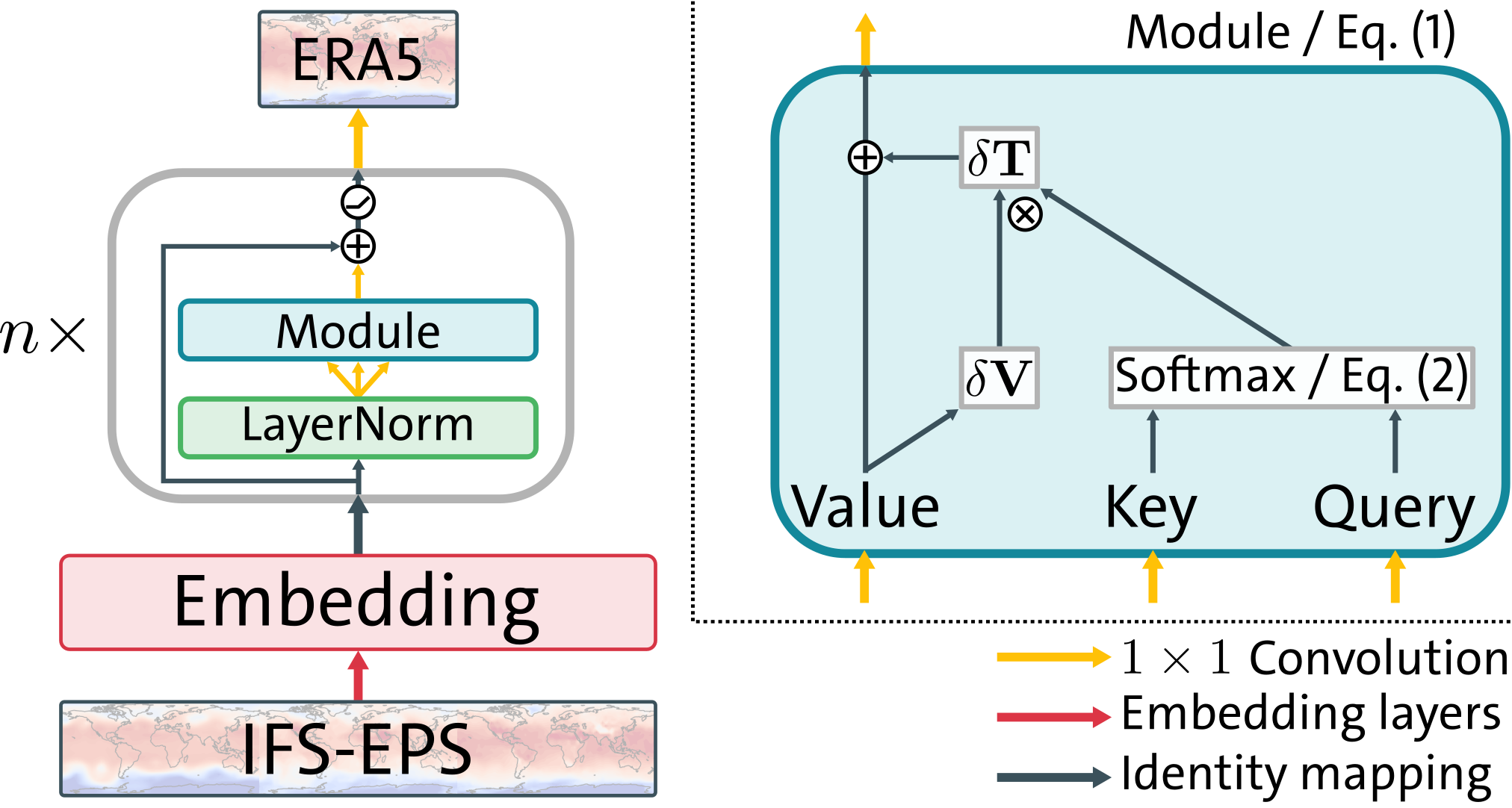
(a) Schematic overview of the ensemble transformer architecture. The separated side of the figure is a zoom-in to a single module.

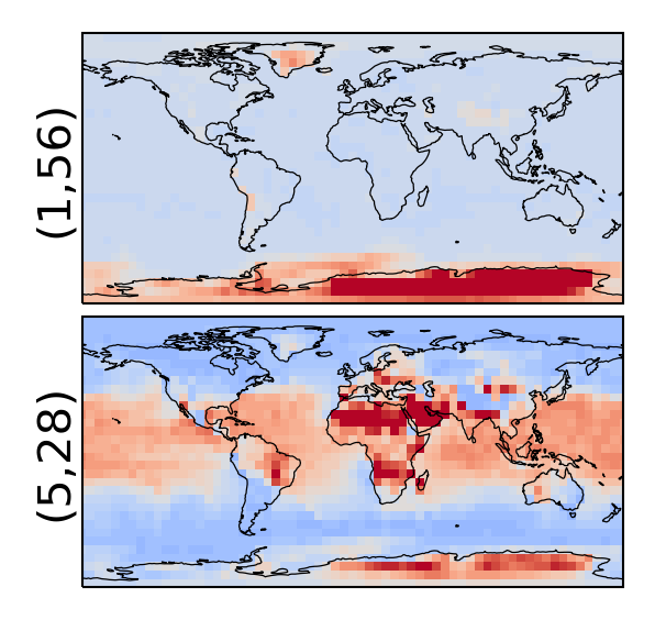
(b) Two selected attention maps (layer number, head number) from the Transformer (5) experiment for 2019-09-01 12:00 UTC. Red (blue) colours indicate a high (low) influence on the attention.

Figure 1: Schematic overview of the self-attentive ensemble transformer architecture and two exemplary attention maps.

I bridge the ideas of the ensemble Kalman filters and self-attention. I introduce the self-attentive ensemble transformer for processing of ensemble data as neural network architecture by stacking multiple self-attention modules. Each module adds to the static value for each ensemble member a dynamic self-attentive part that represents the interactions between ensemble members. As these modules make use of the permutation-invariance of the ensemble members, this type of transformer can be seen as type of set transformer (Lee et al., 2019). To test this idea and compare it to other methods, I regress global ECMWF ensemble forecasts to the 2-metre-temperature of the ERA5 reanalysis project as proof-of-concept experiments.

2 The self-attentive ensemble transformer

In the following, I introduce a single self-attentive transformer module as neural network layer. A schematic overview over the architecture and module can be found in Figure 1(a).

Let ${\bm{{Z}}_{l}\in\mathbb{R}^{k\times c\times h\times w}}$ be the input to the $l$-th layer with $k$ ensemble members, $c$ channels, $h$ latitudes, and $w$ longitudes. The goal of the module is to estimate the transformed output $\bm{{t}}_{i}(\bm{{Z}}_{l})\in\mathbb{R}^{c\times h\times w}$ of the $i$-th member based on the input of all members. The transformed output is split into a static part $\bm{{v}}_{i}$ and a dynamic part $\rm{}_{i}(\bm{{Z}}_{l})$.

The static part, also called value, encodes information that is only dependent on the current $i$-th ensemble member. It is a linear projection of the input $\bm{{V}}=\bm{{Z}}_{l}\bm{{W}}^{v}_{l}$ with a linear projection matrix $\bm{{W}}^{v}_{l}\in\mathbb{R}^{c\times\tilde{c}}$ and $\tilde{c}$ number of channels in the attentive space, also called heads.

The dynamic part adds information from all members to the current $i$-th member. I represent this as additive and linear combination of value perturbations with ensemble weights $\bm{{w}}_{i}\in\mathbb{R}^{k\times\tilde{c}}$ and $\overline{\bm{{v}}}=k^{-1}\sum_{j=1}^{k}\bm{{v}}_{j}$ as the ensemble mean of the values,

$$\bm{{t}}_{i}(\bm{{Z}}_{l})=\bm{{v}}_{i}+\rm_{i}(\bm{{Z}}_{l})=\bm{{v}}_{i}+\sum_{j=1}^{k}\bm{{w}}_{i,j}(\bm{{v}}_{j}-\overline{\bm{{v}}}).$$ (1)

In ensemble data assimilation, the update of ensemble predictions with observations is usually based on a similar parametrization (Bishop et al., 2001; Lorenc, 2003; Hunt et al., 2007). Since no observations are available for post-processing purposes, the transformer module has to rely on self-attention.

In self-attention, the weights are estimated based on the same input data as the values (Vaswani et al., 2017; Wang et al., 2018). Here, the observations are replaced by a query $\bm{{q}}_{i}\in\mathbb{R}^{\tilde{c}\times h\times w}$. The query represents the searched information for the current $i$-th member and is estimated as linear projection of the input data with a projection matrix $\bm{{W}}^{q}_{l}\in\mathbb{R}^{c\times\tilde{c}}$. This query has to be related to the value perturbations of all members to estimate the weights. The relation between query and values is established by a key matrix $\bm{{K}}\in\mathbb{R}^{k\times\tilde{c}\times h\times w}$, which replaces the sensitivity matrix in data assimilation. Again, a linear projection of the input data with a projection matrix $\bm{{W}}^{k}_{l}\in\mathbb{R}^{c\times\tilde{c}}$ is used for the key matrix.

The weight are estimated based on the similarity between the query and key matrix. In correspondence to Vaswani et al. (2017), the similarity is a scaled-dot product $\bm{{K}}(\bm{{q}}_{i})^{T}\in\mathbb{R}^{k\times\tilde{c}}$ over the latitudes and longitudes. To obtain non-negative weights for a convex combination of value perturbations, the scaled-dot product is squashed through a softmax activation,

$$\bm{{w}}_{i} =\frac{\widetilde{\bm{{w}}}_{i}}{\sum_{j=1}^{k}\widetilde{\bm{{w}}}_{i,j}}, \widetilde{\bm{{w}}}_{i}=\exp(\frac{\bm{{K}}(\bm{{q}}_{i})^{T}}{\sqrt{h\times w}}).$$ (2)

These weights make thus explicitly use of the permutation-invariance in self-attention for ensemble data.

I model the output of the transformer module as residual connection (He et al., 2015) with one residual branch and one identity mapping. The residual branch is based on all transformed ensemble members $\bm{{T}}(\bm{{Z}}_{l})\in\mathbb{R}^{k\times\tilde{c}\times h\times w}$, all estimated with (1) at the same time. These transformed ensemble members are linearly projected by $\bm{{W}}^{o}_{l}\in\mathbb{R}^{\tilde{c}\times c}$ from the attentive space back into the original feature space of the identity mapping. I initialize $\bm{{W}}^{o}_{l}$ as all-zero matrix; thus, only the identity mapping is used at the beginning of the training. The output of the residual layer is activated with an activation function $f_{l}$, here the recitified linear unit (ReLU), and results into the input $\bm{{Z}}_{l+1}$ of the next layer,

$$\bm{{Z}}_{l+1}=f_{l}(\bm{{Z}}_{l}+\bm{{T}}(\bm{{Z}}_{l})\bm{{W}}^{o}_{l}).$$ (3)

This finishes the description of a single transformer module.

Since $\rm{}_{i}(\bm{{Z}}_{l})$ is a convex combination of value perturbations, one single-layered ensemble transformer module might be not expressive enough. To extract more complex and non-linear interactions between ensemble members, it might be advantageous to stack multiple modules onto each other.

The ensemble space ($k=50$) is normally much smaller than the spatial space (in my case $h\times w=2048$). Because the weights are estimated in this ensemble space, global self-attention is performed efficiently by (1) and (2). The costs of the ensemble transformer scales quadratically with the number of members, but the weight formulation allows training with another number of members than used for inference as I show later.

The channels $\tilde{c}$ within the attentive space are similar to multiple heads in standard self-attention as the dot product is estimated over spatial dimensions. The channels can thus represent different attentive regions. To discover such regions with high influence, the element-wise product $\overline{\bm{{k}}}\cdot\overline{\bm{{q}}\vphantom{\bm{{k}}}}\in\mathbb{R}^{\tilde{c}\times h\times w}$ of the ensemble mean key $\overline{\bm{{k}}}=k^{-1}\sum_{j=1}^{k}\bm{{k}}_{j}$ and the ensemble mean query $\overline{\bm{{q}}}=k^{-1}\sum_{j=1}^{k}\bm{{q}}_{j}$ can be used. The here-exemplary shown maps (Figure 1(b)) possibly represent regions with temperatures below the freezing level and with heat anomalies.

3 Experiments and Discussion

In a first step, I explain the used architectures and training methods. As second step, I discuss and visualize the results from these experiments.

3.1 Experimental strategy

As input, I use data from the ECMWF ensemble prediction system (IFS-EPS, ECMWF (2019)) with $k=50$ ensemble members and three variables: the geopotential height on the $500\,\text{hPa}$ pressure level, the temperature on the $850\,\text{hPa}$ pressure level, and the 2-metre-temperature. The forecasts with a lead time of 48 hours are valid for 00:00Z and 12:00Z. They are fitted to the 2-metre-temperature of the ERA5 reanalysis project (Hersbach et al., 2020). The whole dataset consists of three-years data (2017-2019): 2017 and 2018 are used for training and validation, whereas 2019 is used for testing purpose. I randomly select $10\,\%$ of 2017 and 2018 for validation. As pre-processing, the global fields are bilinearly regridded to $h\times w=32\times 64$ grid points as in Rasp et al. (2020). The input data is normalized by their global mean and standard deviation, fitted for every variable independently based on the training dataset.

For all of my experiments, I use the same initial embedding structure with three consecutive two-dimensional convolutional layers, which are applied on every ensemble member independently. For these convolutions, I use a kernel size of $5\times 5$ with a locally-equidistant assumption, $c=64$ channels, and the ReLU activation. I circularly pad in longitudinal direction and zero-pad in latitudinal direction.

In the Transformer experiments, I stack $n$ ensemble transformer modules between the embedding and the output. For linear projections within the transformer layers, I use $1\times 1$ convolutions with $\tilde{c}=64$ heads. As proposed in (Xiong et al., 2020), I apply layer normalization (Ba et al., 2016) across the channels, latitudes, and longitudes before the module input is linearly projected. As output layer, I use a $1\times 1$ convolution that combines the information from 64 channels into the 2-metre-temperature for each member independently.

As baseline, I perform to additional experiments with two other approaches. First, I post-process each member independently with a neural network in the Direct experiments. Secondly, I apply a parametric neural network (PPNN, Rasp & Lerch (2018)) that outputs the mean and standard deviation as parameters of a Gaussian distribution. In these parametric networks, the embedding output is averaged over all members and concatenated with the ensemble mean and standard deviation of the inputted 2-metre-temperature, similarly to Rasp & Lerch (2018).

In these baseline experiments, I replace the self-attention modules with $n$ residual layers (He et al., 2015) between embedding and output. These layers are two $1\times 1$ convolutions with $64$ channels and the ReLU activation function in-between. These residual layers have been modified with the fixed-update initialization in correspondence to (Zhang et al., 2019). They are similar to the residual layer within the transformer module without self-attention.

As loss function, I minimize for all experiments the continuously ranked probability score (CRPS, Hersbach (2000); Gneiting & Raftery (2007)) with a Gaussian assumption and latitudinal weighting as in Rasp et al. (2020). For the transformer and direct experiments, I calculate the ensemble mean and the ensemble standard deviation from the resulting ensemble members as CRPS estimation step. I have trained all models on a Nvidia GeForce GTX 1060 with a batch size of 8 samples. Each experiment is optimized with Adam (Kingma & Ba, 2017) and an initial learning rate of $1\times 10^{-3}$. If the validation CRPS is not decreasing for 5 epochs, the learning rate is multiplied with $0.3$ of its previous value. The training is ended if the validation CRPS is not decreasing for 20 epochs or after 200 epochs. I have implemented the models with PyTorch (Paszke et al., 2019).

3.2 Results

To compare the experiments (Table 1 and Table 2), I evaluate the latitudinal weighted spatio-temporal mean CRPS to the ERA5 reanalysis, the weighted spatio-temporal root-mean-squared-error of the ensemble mean (RMSE), and the square-root of the latitudinal weighted spatio-temporal mean of the ensemble variance (Spread). If the ensemble spread is calibrated, it should match the RMSE.

Table 1: The CRPS to the reanalysis, the ensemble mean RMSE, and the mean ensemble spread in the test dataset for all 50 ensemble members. The number behind the experiments indicates how many members were subsampled in each training sample.

Name (members)	CRPS	RMSE (K)	Spread (K)
Transformer (10)	0.42	0.91	0.91
Transformer (20)	0.42	0.92	0.90
Transformer (50)	0.42	0.92	0.89

The training speed depends on the number of ensemble members that are used during the training. To reduce the trainings costs, the ensemble can be subsampled by randomly selecting fewer members for each training sample (Table 1). Because of additional noise, smaller subsampled sizes help to regularize the networks, but a too small subsampled ensemble can lead to an unstable training. To strike a balance, I subsample 20 members in each training sample for all subsequent experiments.

Table 2: The CRPS, the ensemble mean RMSE, and the ensemble standard deviation in the test dataset. The number behind the experiments indicates how many additional layers between embedding and output layer are used. Bold values represent the best performing methods.

Name (layers)	CRPS	RMSE (K)	Spread (K)
Climatology	2.60	6.12	6.05
IFS-EPS raw	0.52	1.12	0.73
PPNN (0)	0.44	0.96	0.87
PPNN (1)	0.43	0.95	0.87
PPNN (5)	0.42	0.93	0.87
Direct (1)	0.45	0.95	0.70
Direct (5)	0.45	0.96	0.70
Transformer (1)	0.42	0.91	0.91
Transformer (5)	0.41	0.90	0.90

The general performance of all methods is bounded by the available information from the input fields as can be seen in Table 2. Nevertheless, the PPNN and Transformer approaches scale slightly with increasing network depth that leads to lower RMSE and CRPS values with increasing number of layers. Since the RMSE of the Transformer experiments is reduced compared to the Direct and PPNN experiments, the self-attention mechanism can extract additional information from the interactions between ensemble members. In addition, the experiments with the Transformer have a perfect spread-skill ratio (a probability integral transform histogram is shown in the Appendix, Figure 3), whereas the ensembles in the Direct experiments are too small and underdispersive. Therefore, the self-attention mechanism enables ensemble calibrations with neural networks and a member-by-member approach. As a result, the ensemble transformer is the best performing method even compared to the parametric PPNN approach.

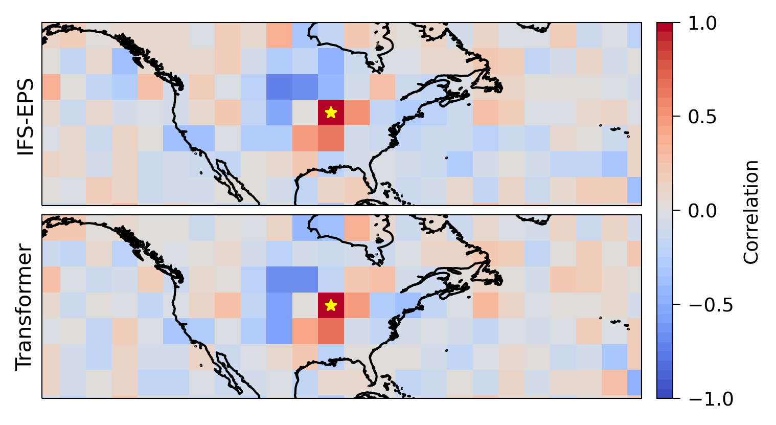
Figure 2: The spatial correlation within the 50 ensemble members from the IFS-EPS data and the Transformer(5) experiment at 26th January 2019, 12:00 UTC, estimated to the yellow-marked grid point of interest, roughly representing the position of Chicago.

Linear spatial patterns within the ensemble members can be found by analysing the ensemble correlation structure (Figure 2). Here, the post-processed ensemble members represent similar correlation structures as they can be found within the raw IFS-EPS ensemble. Normally, additional methods like Gaussian copulas (Schefzik et al., 2013; Lerch et al., 2020) are needed to represent such multivariate structures within a post-processed ensemble. The ensemble transformer is a member-by-member approach and adds interactions between ensemble members as dynamic term. It can thus directly output spatially-coherent ensemble members despite only targeting an univariately spatio-temporal averaged CRPS during training.

4 Conclusion

Based on the results of post-processing global ECMWF ensemble predictions to ERA5 2-metre-temperature reanalyses with ensemble transformers and convolutional neural networks, I conclude the following:

• Self-attention can inform ensemble members about the evolution of other members within a neural network. Global self-attention can be hereby efficiently represented within the space of the ensemble members.

• The ensemble transformer can calibrate the ensemble spread. Furthermore, it can extract additional information from the interactions between ensemble members.

• Ensemble transformer can directly process ensemble members without using ensemble statistics and output again multivariate and spatially-coherent ensemble members.

Therefore, the self-attentive ensemble transformer can be a missing piece for a member-by-member post-processing of ensemble data with neural networks and without using summarized ensemble statistics.

Single model initial-condition large ensembles of climate simulations have to be calibrated (Suarez-Gutierrez et al., 2021) for potential biases in the forced response and internal variability. This study proofs that the training of self-attentive ensemble transformer for global post-processing of Earth system models is possible. By leveraging historical runs and observations, such a transformer can be thus trained to calibrate these single model large ensemble. This could then result in an improved assessment of the forced response and internal variability in the Earth system.

5 Acknowledgements

This work is a contribution to the research unit FOR2131, ”Data Assimilation for Improved Characterization of Fluxes across Compartmental Interfaces”, funded by the ”Deutsche Forschungsgemeinschaft” (DFG, German Research Foundation) under grant 243358811. I would like to acknowledge the ECMWF for providing the IFS-EPS data via the ”The International Grand Global Ensemble” project and the Copernicus Climate Change Service (C3S) for distributing the ERA5 reanalysis data (Hersbach et al., 2020), downloaded from the Climate Data Store. I would like to thank Marc Bocquet, Sebastian Lerch, Laura Suarez-Gutierrez, and two anonymous reviewers for providing insightful remarks and suggestions that helped to improve the manuscript.

References

- Ba et al. (2016) Ba, J. L., Kiros, J. R., and Hinton, G. E. Layer Normalization. ArXiv160706450 Cs Stat, July 2016.
- Baran & Lerch (2018) Baran, S. and Lerch, S. Combining predictive distributions for the statistical post-processing of ensemble forecasts. International Journal of Forecasting, 34(3):477–496, July 2018. ISSN 0169-2070. doi: 10.1016/j.ijforecast.2018.01.005.
- Bauer et al. (2015) Bauer, P., Thorpe, A., and Brunet, G. The quiet revolution of numerical weather prediction. Nature, 525(7567):47–55, 2015. ISSN 1476-4687. doi: 10.1038/nature14956.
- Bishop et al. (2001) Bishop, C. H., Etherton, B. J., and Majumdar, S. J. Adaptive Sampling with the Ensemble Transform Kalman Filter. Part I: Theoretical Aspects. Mon. Wea. Rev., 129(3):420–436, March 2001. ISSN 0027-0644. doi: 10.1175/1520-0493(2001)129¡0420:ASWTET¿2.0.CO;2.
- Bremnes (2020) Bremnes, J. B. Ensemble Postprocessing Using Quantile Function Regression Based on Neural Networks and Bernstein Polynomials. Mon. Weather Rev., 148(1):403–414, January 2020. ISSN 1520-0493, 0027-0644. doi: 10.1175/MWR-D-19-0227.1.
- Burgers et al. (1998) Burgers, G., Jan van Leeuwen, P., and Evensen, G. Analysis Scheme in the Ensemble Kalman Filter. Mon. Wea. Rev., 126(6):1719–1724, June 1998. ISSN 0027-0644. doi: 10.1175/1520-0493(1998)126¡1719:ASITEK¿2.0.CO;2.
- Deser et al. (2020) Deser, C., Lehner, F., Rodgers, K. B., Ault, T., Delworth, T. L., DiNezio, P. N., Fiore, A., Frankignoul, C., Fyfe, J. C., Horton, D. E., Kay, J. E., Knutti, R., Lovenduski, N. S., Marotzke, J., McKinnon, K. A., Minobe, S., Randerson, J., Screen, J. A., Simpson, I. R., and Ting, M. Insights from Earth system model initial-condition large ensembles and future prospects. Nat. Clim. Change, 10(4):277–286, April 2020. ISSN 1758-6798. doi: 10.1038/s41558-020-0731-2.
- ECMWF (2019) ECMWF. IFS Documentation CY46R1. IFS Documentation. 2019.
- Evensen (1994) Evensen, G. Sequential data assimilation with a nonlinear quasi-geostrophic model using Monte Carlo methods to forecast error statistics. J. Geophys. Res. Oceans, 99(C5):10143–10162, 1994. ISSN 2156-2202. doi: 10.1029/94JC00572.
- Gneiting & Raftery (2007) Gneiting, T. and Raftery, A. E. Strictly Proper Scoring Rules, Prediction, and Estimation. Journal of the American Statistical Association, 102(477):359–378, March 2007. ISSN 0162-1459, 1537-274X. doi: 10.1198/016214506000001437.
- Gneiting et al. (2005) Gneiting, T., Raftery, A. E., Westveld, A. H., and Goldman, T. Calibrated Probabilistic Forecasting Using Ensemble Model Output Statistics and Minimum CRPS Estimation. Mon. Weather Rev., 133(5):1098–1118, May 2005. ISSN 1520-0493, 0027-0644. doi: 10.1175/MWR2904.1.
- He et al. (2015) He, K., Zhang, X., Ren, S., and Sun, J. Deep Residual Learning for Image Recognition. ArXiv151203385 Cs, December 2015.
- Hemri et al. (2014) Hemri, S., Scheuerer, M., Pappenberger, F., Bogner, K., and Haiden, T. Trends in the predictive performance of raw ensemble weather forecasts. Geophys. Res. Lett., 41(24):9197–9205, 2014. ISSN 1944-8007. doi: 10.1002/2014GL062472.
- Hersbach (2000) Hersbach, H. Decomposition of the Continuous Ranked Probability Score for Ensemble Prediction Systems. WEATHER Forecast., 15:12, 2000.
- Hersbach et al. (2020) Hersbach, H., Bell, B., Berrisford, P., Hirahara, S., Horányi, A., Muñoz-Sabater, J., Nicolas, J., Peubey, C., Radu, R., Schepers, D., Simmons, A., Soci, C., Abdalla, S., Abellan, X., Balsamo, G., Bechtold, P., Biavati, G., Bidlot, J., Bonavita, M., Chiara, G. D., Dahlgren, P., Dee, D., Diamantakis, M., Dragani, R., Flemming, J., Forbes, R., Fuentes, M., Geer, A., Haimberger, L., Healy, S., Hogan, R. J., Hólm, E., Janisková, M., Keeley, S., Laloyaux, P., Lopez, P., Lupu, C., Radnoti, G., de Rosnay, P., Rozum, I., Vamborg, F., Villaume, S., and Thépaut, J.-N. The ERA5 global reanalysis. Q. J. R. Meteorol. Soc., 146(730):1999–2049, 2020. ISSN 1477-870X. doi: 10.1002/qj.3803.
- Hunt et al. (2007) Hunt, B. R., Kostelich, E. J., and Szunyogh, I. Efficient data assimilation for spatiotemporal chaos: A local ensemble transform Kalman filter. Physica D: Nonlinear Phenomena, 230(1):112–126, June 2007. ISSN 0167-2789. doi: 10.1016/j.physd.2006.11.008.
- Kay et al. (2015) Kay, J. E., Deser, C., Phillips, A., Mai, A., Hannay, C., Strand, G., Arblaster, J. M., Bates, S. C., Danabasoglu, G., Edwards, J., Holland, M., Kushner, P., Lamarque, J.-F., Lawrence, D., Lindsay, K., Middleton, A., Munoz, E., Neale, R., Oleson, K., Polvani, L., and Vertenstein, M. The Community Earth System Model (CESM) Large Ensemble Project: A Community Resource for Studying Climate Change in the Presence of Internal Climate Variability. Bull. Am. Meteorol. Soc., 96(8):1333–1349, August 2015. ISSN 0003-0007, 1520-0477. doi: 10.1175/BAMS-D-13-00255.1.
- Kingma & Ba (2017) Kingma, D. P. and Ba, J. Adam: A Method for Stochastic Optimization. ArXiv14126980 Cs, January 2017.
- Lee et al. (2019) Lee, J., Lee, Y., Kim, J., Kosiorek, A. R., Choi, S., and Teh, Y. W. Set Transformer: A Framework for Attention-based Permutation-Invariant Neural Networks. ArXiv181000825 Cs Stat, May 2019.
- Leith (1974) Leith, C. E. Theoretical Skill of Monte Carlo Forecasts. Mon. Weather Rev., 102(6):409–418, June 1974. ISSN 1520-0493, 0027-0644. doi: 10.1175/1520-0493(1974)102¡0409:TSOMCF¿2.0.CO;2.
- Lerch et al. (2020) Lerch, S., Baran, S., Möller, A., Groß, J., Schefzik, R., Hemri, S., and Graeter, M. Simulation-based comparison of multivariate ensemble post-processing methods. Nonlinear Process. Geophys., 27(2):349–371, June 2020. ISSN 1023-5809. doi: 10.5194/npg-27-349-2020.
- Lorenc (2003) Lorenc, A. C. The potential of the ensemble Kalman filter for NWP—a comparison with 4D-Var. Q. J. R. Meteorol. Soc., 129(595):3183–3203, 2003. ISSN 1477-870X. doi: 10.1256/qj.02.132.
- Luong et al. (2015) Luong, M.-T., Pham, H., and Manning, C. D. Effective Approaches to Attention-based Neural Machine Translation. ArXiv150804025 Cs, September 2015.
- Maher et al. (2019) Maher, N., Milinski, S., Suarez-Gutierrez, L., Botzet, M., Dobrynin, M., Kornblueh, L., Kröger, J., Takano, Y., Ghosh, R., Hedemann, C., Li, C., Li, H., Manzini, E., Notz, D., Putrasahan, D., Boysen, L., Claussen, M., Ilyina, T., Olonscheck, D., Raddatz, T., Stevens, B., and Marotzke, J. The Max Planck Institute Grand Ensemble: Enabling the Exploration of Climate System Variability. J. Adv. Model. Earth Syst., 11(7):2050–2069, 2019. ISSN 1942-2466. doi: 10.1029/2019MS001639.
- Molteni et al. (1996) Molteni, F., Buizza, R., Palmer, T. N., and Petroliagis, T. The ECMWF Ensemble Prediction System: Methodology and validation. Q. J. R. Meteorol. Soc., 122(529):73–119, 1996. ISSN 1477-870X. doi: 10.1002/qj.49712252905.
- Paszke et al. (2019) Paszke, A., Gross, S., Massa, F., Lerer, A., Bradbury, J., Chanan, G., Killeen, T., Lin, Z., Gimelshein, N., Antiga, L., Desmaison, A., Kopf, A., Yang, E., DeVito, Z., Raison, M., Tejani, A., Chilamkurthy, S., Steiner, B., Fang, L., Bai, J., and Chintala, S. PyTorch: An Imperative Style, High-Performance Deep Learning Library. In Wallach, H., Larochelle, H., Beygelzimer, A., Alché-Buc, F., Fox, E., and Garnett, R. (eds.), Advances in Neural Information Processing Systems 32, pp. 8024–8035. Curran Associates, Inc., 2019.
- Raftery et al. (2005) Raftery, A. E., Gneiting, T., Balabdaoui, F., and Polakowski, M. Using Bayesian Model Averaging to Calibrate Forecast Ensembles. Mon. Weather Rev., 133(5):1155–1174, May 2005. ISSN 1520-0493, 0027-0644. doi: 10.1175/MWR2906.1.
- Rasp & Lerch (2018) Rasp, S. and Lerch, S. Neural networks for post-processing ensemble weather forecasts. Mon. Wea. Rev., 146(11):3885–3900, November 2018. ISSN 0027-0644, 1520-0493. doi: 10.1175/MWR-D-18-0187.1.
- Rasp et al. (2020) Rasp, S., Dueben, P. D., Scher, S., Weyn, J. A., Mouatadid, S., and Thuerey, N. WeatherBench: A benchmark dataset for data-driven weather forecasting. ArXiv200200469 Phys. Stat, June 2020.
- Schaeybroeck & Vannitsem (2015) Schaeybroeck, B. V. and Vannitsem, S. Ensemble post-processing using member-by-member approaches: Theoretical aspects. Q. J. R. Meteorol. Soc., 141(688):807–818, 2015. ISSN 1477-870X. doi: 10.1002/qj.2397.
- Schefzik et al. (2013) Schefzik, R., Thorarinsdottir, T. L., and Gneiting, T. Uncertainty Quantification in Complex Simulation Models Using Ensemble Copula Coupling. Stat. Sci., 28(4):616–640, November 2013. ISSN 0883-4237, 2168-8745. doi: 10.1214/13-STS443.
- Scheuerer et al. (2020) Scheuerer, M., Switanek, M. B., Worsnop, R. P., and Hamill, T. M. Using Artificial Neural Networks for Generating Probabilistic Subseasonal Precipitation Forecasts over California. Mon. Weather Rev., 148(8):3489–3506, July 2020. ISSN 1520-0493, 0027-0644. doi: 10.1175/MWR-D-20-0096.1.
- Schulz & Lerch (2021) Schulz, B. and Lerch, S. Machine learning methods for postprocessing ensemble forecasts of wind gusts: A systematic comparison. ArXiv210609512 Phys. Stat, June 2021.
- Steininger et al. (2020) Steininger, M., Abel, D., Ziegler, K., Krause, A., Paeth, H., and Hotho, A. Deep Learning for Climate Model Output Statistics. ArXiv201210394 Phys., December 2020.
- Suarez-Gutierrez et al. (2021) Suarez-Gutierrez, L., Milinski, S., and Maher, N. Exploiting large ensembles for a better yet simpler climate model evaluation. Clim Dyn, May 2021. ISSN 1432-0894. doi: 10.1007/s00382-021-05821-w.
- Taillardat et al. (2016) Taillardat, M., Mestre, O., Zamo, M., and Naveau, P. Calibrated Ensemble Forecasts Using Quantile Regression Forests and Ensemble Model Output Statistics. Mon. Weather Rev., 144(6):2375–2393, June 2016. ISSN 1520-0493, 0027-0644. doi: 10.1175/MWR-D-15-0260.1.
- Toth & Kalnay (1993) Toth, Z. and Kalnay, E. Ensemble Forecasting at NMC: The Generation of Perturbations. Bull. Am. Meteorol. Soc., 74(12):2317–2330, December 1993. ISSN 0003-0007, 1520-0477. doi: 10.1175/1520-0477(1993)074¡2317:EFANTG¿2.0.CO;2.
- Vaswani et al. (2017) Vaswani, A., Shazeer, N., Parmar, N., Uszkoreit, J., Jones, L., Gomez, A. N., Kaiser, L., and Polosukhin, I. Attention Is All You Need. ArXiv170603762 Cs, December 2017.
- Wang et al. (2018) Wang, X., Girshick, R., Gupta, A., and He, K. Non-local Neural Networks. ArXiv171107971 Cs, April 2018.
- Xiong et al. (2020) Xiong, R., Yang, Y., He, D., Zheng, K., Zheng, S., Xing, C., Zhang, H., Lan, Y., Wang, L., and Liu, T. On Layer Normalization in the Transformer Architecture. In International Conference on Machine Learning, pp. 10524–10533. PMLR, November 2020.
- Zhang et al. (2019) Zhang, H., Dauphin, Y. N., and Ma, T. Fixup Initialization: Residual Learning Without Normalization. ArXiv190109321 Cs Stat, March 2019.
Appendix A Additional results