Extreme event propagation using counterfactual theory and vine copulas

Abstract

Understanding multivariate extreme events play a crucial role in managing the risks of complex systems since extremes are governed by their own mechanisms. Conditional on a given variable exceeding a high threshold (e.g. traffic intensity), knowing which high-impact quantities (e.g air pollutant levels) are the most likely to be extreme in the future is key. This article investigates the contribution of marginal extreme events on future extreme events of related quantities. We propose an Extreme Event Propagation framework to maximise counterfactual causation probabilities between a known cause and future high-impact quantities. Extreme value theory provides a tool for modelling upper tails whilst vine copulas are a flexible device for capturing a large variety of joint extremal behaviours. We optimise for the probabilities of causation and apply our framework to a London road traffic and air pollutants dataset. We replicate documented atmospheric mechanisms beyond linear relationships. This provides a new tool for quantifying the propagation of extremes in a large variety of applications.

, and

1 Introduction

Quantifying dependencies between extremes is essential in analysing risk scenarios and extreme chain reactions in applications, e.g. extreme air pollution, meteorology, hydrology (Dutfoy, Parey and Roche, 2014; De Sario, Katsouyanni and Michelozzi, 2013; Bevacqua et al., 2017) or financial risk management (Embrechts, Klüppelberg and Mikosch, 2013). Causal relationships in the context of time series are well-established (Eichler and Didelez, 2007; Eichler, 2013), most notably with the Granger causality (Granger, 1980, 1988) while causality for extremes has shown promising results recently (Kiriliouk and Naveau, 2020; Hannart et al., 2016; Hannart and Naveau, 2018). However, in this case, the temporal evolution of extremes is usually modelled backwards: for instance, the celebrated Extreme Event Attribution (EEA) methodology (Allen, 2003) attributes a particular extreme event to its potential causes (Angélil et al., 2017; Philip et al., 2020; Trenberth, Fasullo and Shepherd, 2015), especially for climate-related applications. In this article, we provide a forward-looking scheme for extremes to investigate the causal impact of an extreme event on a high-impact event through time which we call the Extreme Event Propagation (EEP) framework. This builds upon the peaks-over-thresholds extreme value theory (NERC, 1975; Davison and Smith, 1990; Pickands, 1971) and the counterfactual causal theory (Pearl, 1999).

The peaks-over-thresholds literature takes root in the idea that high values have their own mechanisms and should be treated separately from ordinary values as only those large values provide insights about other extreme values (Rootzén, Segers and L. Wadsworth, 2018). To differentiate ordinary values from extreme ones, a threshold is defined and values above it are considered to be peaks. The excess between the threshold and the peaks have been shown to converge to a generalised Pareto distribution (GPD) (de Haan and Resnick, 1977; Balkema and De Haan, 1974; Pickands, 1971) as the threshold approaches the distribution’s endpoint. A multivariate extension of the GPD (MGPD) was introduced in Beirlant et al. (2004) & Rootzén and Tajvidi (2006). We note that spatial extremes have been instrumental in the development of those extensions (Wadsworth and Tawn, 2018; Bacro et al., 2020), supported by a family of models with an ever-growing distributional and asymptotic flexibility (Wadsworth et al., 2017; Rootzén, Segers and L. Wadsworth, 2018; Kiriliouk et al., 2019). We rely on a copula-based MGPD definition presented in Falk, Padoan and Wisheckel (2019), where marginal distributions have GPD upper tails and are all together linked through a threshold-stable copula structure called a generalised Pareto copula.

On the other hand, the counterfactual causal theory (Pearl, 1999) relies on a cause event and an impact event and opposes two versions of the world: the factual world where the cause happened, and the counterfactual one where it did not. We compare those settings through three combined probabilities, called probabilities of causation, to quantify and potentially maximise the necessary or sufficient nature of the cause on the impact event, see Naveau, Hannart and Ribes (2020) for a recent statistical review. Hannart and Naveau (2018) and Kiriliouk and Naveau (2020) apply this approach to extreme values for atmospheric applications. The EEP framework is an extension of their idea where we model both the cross-sectional and temporal dependencies, bringing the analysis a step closer to handling realistic risk management situations. Alternatively, Gnecco et al. (2019) define a causal tail coefficient that captures asymmetries in the extremal dependence of two random variables and Mhalla, Chavez-Demoulin and Dupuis (2020) construct an information-theoretic statistic to uncover causal links.

Although the cause and impact events can be tailored to the application at hand (Philip et al., 2020; Hannart and Naveau, 2018), we also describe our framework with parametrised cause and impact events. For instance, Bevacqua et al. (2017) introduces compound events where the individual variables may not be extreme themselves but their joint occurrence causes an extreme impact—a case that is therefore covered in the EEP framework. On the other hand, Hannart et al. (2016) maximises a probability of causation with respect to an extreme temperature threshold, delimiting high values from ordinary ones. This also allows for the discovery of causal links between the cause and individual variables through time as an alternative to the pairwise approaches (Peters et al., 2014; Mhalla, Chavez-Demoulin and Dupuis, 2020; Gnecco et al., 2019) or sparse structures for extremes (Engelke and Ivanovs, 2021; Engelke and Volgushev, 2019; Engelke and Hitz, 2020) that extract the most significant extremal pairwise links in a tractable manner.

Modelling extremal behaviour accurately requires flexible dependence structures as formalised by the asymptotic dependence (Wadsworth et al., 2017; Huser and Wadsworth, 2019), regularly varying distributions (Mikosch, 2006; Weng and Zhang, 2012) or sparse structures for high-dimensions (Engelke and Ivanovs, 2021; Engelke and Hitz, 2020). Although the EEP framework remains model-agnostic in its current formulation, vine copulas (Bedford and Cooke, 2002)—a family of hierarchical pairwise graphical copulas—are a balance between adjustable extremal properties (Joe, Li and Nikoloulopoulos, 2010), the ability to capture non-linear relationships (Gräler, 2014; Erhardt, Czado and Schepsmeier, 2015) and scalability capabilities (Nagler, Bumann and Czado, 2018; Nagler, Krüger and Min, 2020). It also offers a conditional sampling mechanism (Bevacqua et al., 2017, App. B), a key ingredient for counterfactual reasoning (Eichler, 2013, Section 2.b).

After a short presentation of counterfactual theory and time-series causality, we introduce the components of the EEP framework in Section 2: the cause and impact events as well as the counterfactual probabilistic setting to understand their causal link. In Section 3, we recall the properties of interest for multivariate extremes modelling related to copulas and define the semiparametric and counterfactual marginal model used. The model inference is deferred to Section 4 where marginal parameters are obtained by maximum likelihood whilst extreme thresholds are chosen by sequential hypothesis testing. We also mention different inference approaches for vine copulas such as a tree structure selection algorithm and model selection criteria. Tail probabilities are essential quantities in counterfactual settings and we introducing a marginal transformation approach to handle the cross-sectional comparisons of potentially different quantities in nature. Finally, Section 5 is devoted to presenting a case study about the impact of high road traffic on air pollutant concentration peaks in the following six hours on Bloomsbury Road, London (UK). An overview of causality for time series and shortlisted definitions from the counterfactual causal theory and vine copulas literature are presented in Appendix B– D.

2 Extreme Event Propagation

Starting with Allen (2003), the EEA literature focuses on determining if climate change influenced the frequency, likelihood, and/or severity of individual extreme events (Swain et al., 2020, p. 525).

We are interested in modelling the opposite, that is, how the conditions linked to an extreme event taking place can propagate through time and cross-sections to increase the probability of another, potentially higher-impact, extreme event. Also, we quantify which of the marginals involved in this impact event are more likely to reach extreme levels in the future. We call this the Extreme Event Propagation (EEP) framework.

2.1 Foundations

EEP applies the causal counterfactual theory (Pearl, 1999) to assess how a quantity above a high threshold at a given time can impact a collection of target variables to become extreme later in time.

In this article, we oppose a factual version of the world (i.e. where the cause intervenes on the system under study) and counterfactual version (i.e. where it does not intervene) version to observe and potentially maximise a given probability of causation of the potential cause on a parametrised impact event. We decompose the EEP framework into three steps:

1. defining the cause i.e. the factual and counterfactual worlds;

2. defining the (parametrised) impact event;

3. comparing those settings through a probabilistic causal framework;

analogously to the EEA framework (Swain et al., 2020; Philip et al., 2020).

2.2 Notations

Let $I=\{1,\dots,d\}$ be an index set for the $d\in\mathbb{N}$ variables. On a filtered probability space $(\Omega,\mathcal{F},\{\mathcal{F}_{t},\ t\in{\mathbb{N}}\},{\text{P}})$, we consider an adapted and strictly stationary $d$-dimensional process

$$\mathbb{X}_{t}=({\textnormal{X}}^{1}_{t},\dots,{\textnormal{X}}^{d}_{t})^{\top},\quad t\in\mathbb{N},$$

where we simplify the usual marginal notation ${\textnormal{X}}^{(i)}$ into ${\textnormal{X}}^{i}$ for conciseness. We write $F$ the cdf (resp. $f$ the pdf) of $\mathbb{X}$; $F^{i}$ the cdf (resp. $f^{i}$ the pdf) of ${\textnormal{X}}^{i}$ for $i\in I$. In addition, we write the quantile function (or generalised inverse) of a univariate distribution $F^{i}$ by $Q^{i}(u)\overset{\Delta}{=}\inf\left\{t\in\mathbb{R}:F(t)\geq u\right\}$ for $u\in[0,1]$. For an offset index $k\in\mathbb{N}$, we denote the forward-looking $k$-stack of $\mathbb{X}_{t},\dots,\mathbb{X}_{t+k}$ by

$$\mathbb{X}_{t}(k)\overset{\Delta}{=}(\mathbb{X}_{t}^{\top},\dots,\mathbb{X}_{t+k}^{\top})^{\top}\in\mathbb{R}^{(k+1)d}.$$

The integral transform is given by ${\textnormal{U}}^{i}_{t}\overset{\Delta}{=}F^{i}({\textnormal{U}}^{i}_{t})\sim\mathcal{U}(0,1),$ and we define

$$\mathbb{U}_{t}\overset{\Delta}{=}(U^{i}_{t},\ i\in I)\in(0,1)^{d},\quad\text{and}\quad\mathbb{U}_{t}(k)\overset{\Delta}{=}(\mathbb{U}_{t}^{\top},\dots,\mathbb{U}_{t+k}^{\top})^{\top}\in(0,1)^{(k+1)d}.$$

The generalised Pareto distribution (GPD) with threshold $u$, shape $\gamma\in\mathbb{R}$ and scale $\sigma>0$, denoted $\mathrm{GPD}(u,\gamma,\sigma)$, has a pdf given by

$$f(x;\gamma,\sigma,u)=\sigma^{-1}\left(1+\frac{\gamma}{\sigma}(x-u)\right)_{+}^{-1/\gamma},$$

where $x_{+}\overset{\Delta}{=}\max(x,0)$. If $u=0$, we simply denote this distribution by $\mathrm{GPD}(\gamma,\sigma)$.

2.3 The cause

We are interested in quantifying the contribution of individual variables on the impact event and consider the $i$-th marginal extreme event denoted by

$${\bm{C}}_{t}^{i}\overset{\Delta}{=}{\bm{C}}_{t}(\mu^{i},\bm{e}^{i}_{d})=\{X^{i}_{t}>\mu^{i}\},\quad\text{for some $\mu^{i}\in\mathbb{R}$,}\quad i\in I,$$ (1)

where $\bm{e}^{i}_{d}=(0,\dots,0,1,0,\dots,0)^{\top}\in\mathbb{R}^{d}$ is the $i$-th standard unit vector in $\mathbb{R}^{d}$. The specific value chosen for $\mu^{i}$ is a threshold value above which ${\textnormal{X}}^{i}$ is said to be extreme and is formally defined in Section 3.2.

2.4 The impact event

We define an impact function $h=h(\bm{x};{\bm{w}}):\mathbb{R}^{p+m}\rightarrow\mathbb{R}$ for $p,m\in\mathbb{N}$ where $\bm{x}\in\mathbb{R}^{p}$ are the variables whilst the vector ${\bm{w}}\in\mathbb{R}^{m}$ parametrise the function $h$ (Bevacqua et al., 2017). To simplify the notation, we allow for different values of $p$ and $m$ in the definition of $h$ when the context is clearly defined.

We consider the event of $h\left(\mathbb{X}_{t}(k);{\bm{w}}\right)$ taking its value above a high threshold $v\in{\mathbb{R}}$ for some parameter vector ${\bm{w}}\in(0,\infty)^{m}$, denoted

$${\bm{E}}_{t}(v,{\bm{w}},k;h)\overset{\Delta}{=}\left\{h(\mathbb{X}_{t+1}(k);{\bm{w}})>v\right\},\quad{\bm{w}}\in[0,\infty)^{m},\quad k\in{\mathbb{N}},$$

which we call the impact event of $\mathbb{X}$ at time $t+k$ with respect to the threshold $v$ and impact function $h$.

Remark 1.

The impact function was originally introduced by Bevacqua et al. (2017) to study compound events where individual variables may not be extreme but a collection of those variables can cause some extreme impact.

Definition 1.

A measurable function $L:[0,\infty)\mapsto[0,\infty)$ for which the limit $g(a)=\lim_{x\rightarrow\infty}L(ax)/L(x)$ exists and is finite for all $a>0$, is called regularly varying. If $g(a)=1$ for all $a>0$, then $L$ is called slowly varying.

2.4.1 Linear impact events

The multivariate regular variation (MRV) property is an important tool to model multivariate heavy-tailed phenomena (de Haan and Resnick, 1977). See Chapter 5, Resnick (1987) for additional information on the MRV property. We leverage a key characterisation of the MRV property (Basrak, Davis and Mikosch, 2002) which states that any random vector $\mathbb{Y}\in\mathbb{R}^{m}$ satisfies the MRV property if and only if every linear combination of the random vector is (univariate) regularly varying: that is, if there exists a $\beta>0$ and a slowly varying function $L$ such that, for all ${\bm{w}}\in\mathbb{R}^{m}$, the limit

$$\lim_{u\rightarrow\infty}\frac{{\text{P}}({\bm{w}}^{\top}\mathbb{Y}>u)}{u^{-\beta}L(u)}\quad\text{exists,}$$

and there exists some ${\bm{w}}_{0}\neq\bm{0}$ such that the limit is non-zero. Therefore, if the MRV property holds for the multivariate distribution of $\mathbb{X}_{t}(k)$, then, ${\bm{w}}^{\top}\mathbb{X}_{t+1}(k)$ is regularly varying as a marginal distribution, irrespective of the weight vector ${\bm{w}}$.

Therefore, we only investigate the weighted sum impact function which is denoted by

$$h_{\mathrm{sum}}({\bm{y}},{\bm{w}})={\bm{w}}^{\top}{\bm{y}},\quad\text{for }{\bm{y}}\in\mathbb{R}^{m}.$$

Conveniently, this helps us separate the methodology that we introduce with the modelling of impact events which is beyond the scope of this article. We define the family of linear impact events with all marginals between times $t+1$ and $t+k$ as follows

$${\bm{E}}_{t}(v,{\bm{w}},k)\overset{\Delta}{=}\left\{{\bm{w}}^{\top}\mathbb{X}_{t+1}(k)>v\right\},\quad{\bm{w}}\in[0,\infty)^{kd},\quad k\in{\mathbb{N}},$$ (2)

where $\mathbb{X}_{t+1}(k)=(\mathbb{X}_{t+1}^{\top},\dots,\mathbb{X}_{t+k}^{\top})^{\top}\in\mathbb{R}^{kd}$ such that ${\bm{E}}_{t}(v,{\bm{w}},k)\in{\mathcal{F}}_{t+k}$.

2.4.2 Examples

We denote by $\bm{e}^{i}_{m}=(0,\dots,0,1,0,\dots,0)^{\top}\in\mathbb{R}^{m}$ the $i$-th standard unit vector in $\mathbb{R}^{m}$ and by $\otimes$ the Kronecker product.

Cross-sectional impact event

For $l\in\{1,\dots,k\}$ and a weight vector ${\bm{w}}^{l}_{d}\in[0,\infty)^{d}$, the impact event of the cross-sectional combination of $\mathbb{X}$ at time $t+l$ is given by

$${\bm{E}}_{t+l}(v,{\bm{w}}^{l}_{d})\overset{\Delta}{=}{\bm{E}}_{t}(v,{\bm{e}}^{l}_{k}\otimes{\bm{w}}^{l}_{d},k)=\left\{{{\bm{w}}^{l}_{d}}^{\top}\mathbb{X}_{t+l}>v\right\}=\left\{\sum_{i=1}^{d}{\bm{w}}^{l,i}_{d}X^{i}_{t+l}>v\right\},$$ (3)

similarly to the framework of Kiriliouk and Naveau (2020) such that ${\bm{E}}_{t}(v,{\bm{w}}^{l}_{d},k)\in{\mathcal{F}}_{t+l}\subseteq{\mathcal{F}}_{t+k}$.

Timewise marginal impact event

For $j\in\{1,\dots,d\}$ and a weight vector ${\bm{w}}^{j}_{k}\in[0,\infty)^{k}$, the $j$-th timewise marginal impact event between $t+1$ and $t+k$ is defined by

$${\bm{E}}^{j}_{t}(v,{\bm{w}}^{j}_{k},k)\overset{\Delta}{=}{\bm{E}}_{t}(v,{\bm{w}}^{j}_{k}\otimes{\bm{e}}^{j}_{d},k)=\left\{{{\bm{w}}^{j}_{k}}^{\top}\mathbb{X}^{j}_{t+1}(k)>v\right\}=\left\{\sum_{l=1}^{k}{\bm{w}}^{j,l}_{k}X^{j}_{t+l}>v\right\},$$ (4)

where $\mathbb{X}^{j}_{t+1}(k)=(X^{j}_{t+1},\dots,X^{j}_{t+k})^{\top}\in\mathbb{R}^{k}$ and ${\bm{E}}^{j}_{t}(v,{\bm{w}}^{j}_{k},k)\in{\mathcal{F}}_{t+k}$. In this case, we are interested in the temporal changes specific to the $j$-th marginal.

2.5 Causal probabilities

Consider a cause event ${\bm{C}}_{t}\in{\mathcal{F}}_{t}$ from Section 2.3 (e.g. peak traffic level at time $t$) and an impact event ${\bm{E}}_{t}(k)\in{\mathcal{F}}_{t+k}$ from Section 2.4 (e.g. air pollutant levels up to time $t+k$).

2.5.1 Probabilities of causation

Using the do-notation of Pearl (1999), the $\mathrm{PC}$s are defined and given as follows:

$$\mathrm{PN}(k)\ \overset{\Delta}{=}\ {\text{P}}\big{(}{\bm{E}}(k)^{c}\ |\ do({\bm{C}}^{c}),{\bm{C}},{\bm{E}}(k)\big{)}\quad$$ (necessary),

$$\mathrm{PS}(k)\ \overset{\Delta}{=}\ {\text{P}}\big{(}{\bm{E}}(k)\ |\ do({\bm{C}}),{\bm{C}}^{c},{\bm{E}}(k)^{c}\big{)},\quad$$ (sufficient),

$$\mathrm{PNS}(k)\ \overset{\Delta}{=}\ {\text{P}}\big{(}\{{\bm{E}}(k)\ |\ do({\bm{C}})\}\cap\{{\bm{E}}(k)\ |\ do({\bm{C}}^{c})\}\big{)},\quad$$ (sufficient and necessary).

The probability of necessary causation $(\mathrm{PN})$ represents how likely it is that the event ${\bm{E}}(k)$ has not occurred had the cause ${\bm{C}}$ not occurred itself, given that both the event ${\bm{E}}(k)$ and the cause ${\bm{C}}$ have actually occurred. On the other hand, the probability of sufficient causation $(\mathrm{PS})$ quantifies how probable the impact event ${\bm{E}}(k)$ would have occurred in the presence of the cause, given that neither the impact event and the cause have occurred. Finally, the probability of necessary and sufficient causation $(\mathrm{PNS})$ represents how likely it is that the impact event occurs in the presence of the cause and would not occur in the absence of the cause.

2.5.2 Counterfactual probabilities

We derive the probability of necessary causation with respect to impact events described in Section 2.4. For the corresponding cause ${\bm{C}}^{i}$, the probability of ${\bm{E}}(v,{\bm{w}},k)$ is denoted by

$$p^{(i)}_{\mathrm{f}}(v,{\bm{w}};k)\ \overset{\Delta}{=}\quad{\text{P}}\left({\bm{E}}(v,{\bm{w}},k)\ |\ {\bm{C}}^{i}\right), \text{in the \emph{factual} world},$$

$$p^{(i)}_{\mathrm{cf}}(v,{\bm{w}};k)\ \overset{\Delta}{=}\quad{\text{P}}\left({\bm{E}}(v,{\bm{w}},k)\ |\ {\bm{C}}^{i,c}\right), \text{in the \emph{counterfactual} world},$$

where the time index $t$ is omitted since $\mathbb{X}$ is stationary. Those are called factual and counterfactual probabilities, respectively: that ${\bm{w}}^{\top}\mathbb{X}_{1}(k)=\sum_{l=1}^{k}\sum_{j=1}^{d}w_{(l-1)d+j}\mathbb{X}^{j}_{l}$ is above a threshold $v$ given that the $i$-th dimension was extreme (resp. not extreme) at time $0$.

Furthermore, we assume that ${\bm{C}}^{i}$ is exogenous with respect to ${\bm{E}}(k)$ and that ${\bm{E}}(k)$ is monotonous with respect to ${\bm{C}}^{i}$ (Pearl, 1999, Def. 13 & 14), such that $\mathrm{PN}$, $\mathrm{PN}$ and $\mathrm{PNS}$ are all identifiable (Pearl, 1999, Def. 15). For $v\in\mathbb{R}$ and ${\bm{w}}\in[0,\infty)^{kd}$, the corresponding (counter)factual probabilities are defined by

$$p^{(i)}_{\mathrm{f}}(v,{\bm{w}};k) ={\text{P}}\left({\bm{w}}^{\top}\mathbb{X}_{1}(k)>v\ \big{|}\ {\textnormal{X}}^{i}_{0}>\mu^{i}\right),$$ (5)

$$p^{(i)}_{\mathrm{cf}}(v,{\bm{w}};k) ={\text{P}}\left({\bm{w}}^{\top}\mathbb{X}_{1}(k)>v\big{|}\ {\textnormal{X}}^{i}_{0}\leq\mu^{i}\right),$$ (6)

that is, the probability that ${\bm{w}}^{\top}\mathbb{X}_{1}(k)=\sum_{l=1}^{k}\sum_{j=1}^{d}w_{(l-1)d+j}\mathbb{X}^{j}_{l}$ is above a threshold $v$ given that the $i$-th dimension was extreme (resp. not extreme) at time $0$. For a general weight vector ${\bm{w}}\in[0,\infty)^{kd}$, the corresponding PCs are given by

$$\mathrm{PN}^{(i)}(v,{\bm{w}};k)=\left(1-\frac{p^{(i)}_{\mathrm{cf}}(v,{\bm{w}};k)}{p^{(i)}_{\mathrm{f}}(v,{\bm{w}};k)}\right)_{+}, \quad\quad\mathrm{PS}^{(i)}(v,{\bm{w}};k)=\left(1-\frac{1-p^{(i)}_{\mathrm{f}}(v,{\bm{w}};k)}{1-p^{(i)}_{\mathrm{cf}}(v,{\bm{w}};k)}\right)_{+},$$

and

$$\mathrm{PNS}^{(i)}(v,{\bm{w}};k)=\Big{(}p^{(i)}_{\mathrm{cf}}(v,{\bm{w}};k)-p^{(i)}_{\mathrm{f}}(v,{\bm{w}};k)\Big{)}_{+},$$

where $x_{+}=\max(x,0)$ as given in Eq. (8), Hannart et al. (2016). However, the PCs quantify in three different ways the relationship of the cause on the impact events which we believe are better suited to reflect the complex mechanisms involved in the propagation of extremes. That is, they gain value when presented jointly (see Section 5 and Pearl (1999)).

Remark 2.

Hannart and Naveau (2018) studies the impact of PNS to uncover causal links between a cause and a parametrisable impact event whilst Kiriliouk and Naveau (2020) focus on maximising PN to attribute weather precipitation to anthropogenic forcings (i.e. human influence).

To estimate factual and counterfactual probabilities, we model the relationships between the marginals at different times using stationary vine copulas (Nagler, Krüger and Min, 2020), see Section D. In the following section, we detail the motivation behind the use of this model class as well as the different modelling approaches and the estimation schemes available to compute such probabilities.

3 Modelling multivariate extreme values

For some fixed $k\in\mathbb{N}$, we consider a strictly stationary $\mathbb{R}^{d}$-valued time series $(\mathbb{X}_{t},\ t\in\mathbb{N})$ whose $k$-stack $(\mathbb{X}_{t}(k),\ t\in\mathbb{N})$ has a distribution function denoted by $F$ in the $\delta$-neighbourhood of a Multivariate Generalised Pareto Distribution (MGPD) (Falk, Padoan and Wisheckel, 2019, Definition 1) as recalled in the following section. We then introduce our modelling approach based on Archimedean stationary vine copulas (Bedford and Cooke, 2001, 2002).

3.1 Tail dependence modelling

Heffernan and Tawn (2004) set a precedent by outlining a flexible multivariate extreme value framework capable to capture a wide range of tail dependencies. We introduce the dependency measures and succinct theoretical justifications that stationary vine copulas are suitable to model those asymptotic behaviours.

3.1.1 Asymptotic dependence of extremes

Similarly to an upper tail dependence coefficient, we introduce a modified extremal correlation (Engelke and Volgushev, 2019, Eq. (9)) at horizon $h\in\mathbb{N}$ on a set index $S\subseteq I$ as follows

$$\chi^{(i)}(S;h)\overset{\Delta}{=}\lim_{u\uparrow 1}{\text{P}}\left(X^{j}_{h}>Q^{j}(u),\ \forall j\in S\ \big{|}\ X^{i}_{0}>Q^{i}(u)\right),\quad\forall i\in I,$$

and, in particular, the pairwise tail coefficients are given by $\chi^{(i,j)}(h)\overset{\Delta}{=}\chi^{(i)}(\{j\};h)$ for $i,j\in I$. The latter quantifies the joint extremal behaviour of the $j$-th component as the $i$-th component becomes high with a time difference $h$.

If $\chi^{(i,j)}(h)=0$, we say that $X^{i}$ and $X^{j}$ are asymptotically independent at horizon $h$. Otherwise, if $0<\chi^{(i,j)}(h)<1$, they are said to be asymptotically dependent and for $\chi^{(i,j)}(h)=1$ they are completely extremal dependent (Coles, Heffernan and Tawn, 1999; Schlather and Tawn, 2003). However, the tail coefficients do not characterise the extremal dependence structure of $\mathbb{X}_{t}(k)$, see Section 8.1, Mikosch (2006). add details back?

Some recent models have the limitation that either $\chi^{(i,j)}(h)=0$ or $\chi^{(i,j)}(h)>0$ for all $i,j\in I$ and some fixed $h\in\mathbb{N}$ (Huser and Wadsworth, 2019; Kiriliouk et al., 2019) whereas some models avoid this issue (Winter and Tawn, 2017, 2016) by allowing for a mixture of both zero and positive pairwise tail coefficients. Similarly, our model goes in this direction as regular vines adapt their structure to accommodate some pairwise tail coefficients to be zero and others to be positive (Section 3.2.6).

3.1.2 Tail dependence functions

Suppose $C=C({\bm{u}})$ is an $m$-dimensional copula. Denote by $C_{S}$ the marginal copula function of the subset of variables indexed by $S\subseteq\{1,\dots,m\}$ (e.g. $C_{\{1,\dots,m\}}=C$ and $C_{\{i\}}=\text{id}_{[0,1]}$) and by $\bar{C}_{S}$ the survival function of $C_{S}$. Similarly, denote by ${\bm{u}}_{S}=(u_{i},\ i\in S)$ the vector ${\bm{u}}\geq\bm{0}\in\mathbb{R}^{m}$ indexed by $S$ and let $S_{1},S_{2}\subseteq\{1,\dots,m\}$. The upper tail dependence, exponent and conditional tail dependence functions of $C$ are defined by

$$b^{*}_{S}({\bm{u}};C)\quad \overset{\Delta}{=}\quad\lim_{x\downarrow 0}\quad x^{-1}\bar{C}_{S}(\bm{1}-x{\bm{u}}_{S}),$$ (upper tail dependence)

$$a^{*}({\bm{u}};C)\quad \overset{\Delta}{=}\quad\sum_{\begin{subarray}{c}S\subseteq\{1,\dots,m\}:\\ S\neq\emptyset\end{subarray}}(-1)^{|S|-1}b^{*}_{S}({\bm{u}}_{S};C),$$ (upper exponent)

In particular, if $S=\{j\}$ for some $j\in\{1,\dots,m\}$, we define $b^{*}_{j}({\bm{u}};C)=b^{*}_{\{j\}}({\bm{u}};C)=u_{j}$. Note that if $C$ has continuous second-order partial derivatives, we have

$$a^{*}({\bm{u}};C)=\lim_{x\downarrow 0}x^{-1}{\text{P}}\left(U_{i}\geq 1-xu_{i},\text{ for some $i\in I$}\right),$$

by the inclusion-exclusion principle.

3.2 Multivariate Generalised Pareto distribution

We suppose that, for any $t\in\mathbb{N}$, the distribution function of $(X^{i}_{t},\ i\in I)$ is in the domain of attraction of a multivariate non-degenerate distribution $G_{t}=G$, written $F\in\mathcal{D}(G)$, if there are vectors $\bm{a}_{n}>\bm{0}\in\mathbb{R}^{d}$, $\bm{b}_{n}\in\mathbb{R}^{d}$ and $n\in\mathbb{N}$ such that

$$F^{n}(\bm{a}_{n}\bm{x}+\bm{b}_{n})\rightarrow G(\bm{x}),\quad n\rightarrow\infty,$$

for every continuity point $\bm{x}\in\mathbb{R}^{d}$ of $G$ where the vector operations and inequalities are meant componentwise. Note that $G$ is necessarily max-stable, i.e. there exist vectors $\bm{a}_{n}>\bm{0}\in\mathbb{R}^{d}$, $\bm{b}_{n}\in\mathbb{R}^{d}$ and $n\in\mathbb{N}$ such that $G^{n}(\bm{a}_{n}\bm{x}+\bm{b}_{n})=G(\bm{x})$ for any $\bm{x}\in\mathbb{R}^{d}$. By Sklar’s theorem (Sklar, 1959), there exists a function $C:[0,1]^{d}\rightarrow[0,1]$ such that

$$F(x^{1},\dots,x^{d})=C\left(F^{1}(x^{1}),\dots,F^{d}(x^{d})\right),\quad\text{for all }\bm{x}\in\mathbb{R}^{d},$$

and $C$ is called the copula of $F$. Also, if $F$ is continuous then $C$ is unique.

We suppose that the distribution of the $k$-stack $(\mathbb{X}_{t}(k),\ t\in\mathbb{N})$ is in the $\delta$-neighbourhood of a multivariate generalised Pareto distribution ($\mathrm{MGPD}$) (Falk, Padoan and Wisheckel, 2019, Definition 1) which entails

1. marginal distributions of $\mathbb{X}$ have GPD upper tails;

2. there exists a generalised Pareto copula (GPC) $C_{D}$ modelling the joint extremes of $\mathbb{X}_{t}(k)$;

3. $C$ is in the $\delta$-neighbourhood of $C_{D}$ for some $\delta>0$;

which we formalise in the following sections. Alternative $\mathrm{MGPD}$ formulations include generator-based distributions (Rootzén, Segers and L. Wadsworth, 2018; Kiriliouk et al., 2019) where extremes events happen when at least one of the components is above a high threshold.

3.2.1 Marginal upper tails

According to the peaks-over-threshold methodology (Davison and Smith, 1990), for any $i,j\in I$, we suppose that there are thresholds $\mu^{i,j}_{\mathrm{f}}(l)$ and $\mu^{i,j}_{\mathrm{cf}}(l)$ in $\mathbb{R}$ sufficiently high such that

$${\textnormal{X}}^{j}_{l}\ |\ {\textnormal{X}}^{j}_{l}>\mu^{i,j}_{\mathrm{f}}(l),\ {\bm{C}}^{i}\ \sim\mathrm{GPD}\left(\mu^{i,j}_{\mathrm{f}}(l),\gamma^{i,j}_{\mathrm{f}}(l),\sigma^{i,j}_{\mathrm{f}}(l)\right), l\in\mathbb{N}\cup\{0\},$$ (factual)

$${\textnormal{X}}^{j}_{l}\ |\ {\textnormal{X}}^{j}_{l}>\mu^{i,j}_{\mathrm{cf}}(l),\ {\bm{C}}^{i,c}\sim\mathrm{GPD}\left(\mu^{i,j}_{\mathrm{cf}}(l),\gamma^{i,j}_{\mathrm{cf}}(l),\sigma^{i,j}_{\mathrm{cf}}(l)\right), l\in\mathbb{N},$$ (counterfactual)

with shape parameters $\gamma^{i,j}_{\mathrm{f}}(l),\gamma^{i,j}_{\mathrm{cf}}(l)\in\mathbb{R}$ and scale parameters $\sigma^{i,j}_{\mathrm{f}}(l),\sigma^{i,j}_{\mathrm{cf}}(l)>0$. We denote by

$${\bm{\mu}}^{i}_{\mathrm{f}}(l)\overset{\Delta}{=}(\mu^{i,1}_{\mathrm{f}}(l),\dots,\mu^{i,d}_{\mathrm{f}}(l))^{\top}\in\mathbb{R}^{d},\quad\text{and}\quad{\bm{\mu}}^{i}_{\mathrm{cf}}(l)\overset{\Delta}{=}(\mu^{i,1}_{\mathrm{cf}}(l),\dots,\mu^{i,d}_{\mathrm{cf}}(l))^{\top}\in\mathbb{R}^{d},$$

the vector of factual and counterfactual extreme thresholds. The quantile thresholds and vectors are defined by

$$\mu^{i,j}_{0,\cdot}(l)\overset{\Delta}{=}{\text{P}}(X^{j}_{l}\leq\mu^{i,j}_{\cdot}(l)\ |\ {\bm{C}}^{i})\quad\text{and}\quad{\bm{\mu}}^{i}_{0,\cdot}(l)\overset{\Delta}{=}(\mu^{i,1}_{0,\cdot}(l),\dots,\mu^{i,d}_{0,\cdot}(l))^{\top}.$$ (7)

3.2.2 Generalised Pareto Copulas

Deheuvels (1984) & Galambos (1987) showed that $F\in\mathcal{D}(G)$ if and only if it is the case marginally, i.e. $F^{i}\in\mathcal{D}(G^{i})$, as well as for the copula $C$. The latter is equivalent to $C^{n}({\bm{u}}^{1/n})\rightarrow G^{*}(-\log{\bm{u}})$, as $n\rightarrow\infty$, where ${\bm{u}}\in(0,1]^{m}$ and $G^{*}$ is a max-stable distribution with standard negative exponential margins. Th. 2.3.3, Falk (2019) yields that this class of distributions can be formulated as follows

$$G^{*}({\bm{x}})=\exp\left(-\|{\bm{x}}\|_{D}\right),\quad{\bm{x}}\in\mathbb{R}^{m},$$

where $\|\cdot\|_{D}$ is a $D$-norm ($D$ for dependence) (de Haan and Resnick, 1977; Pickands, 1989) which are characterised by a generator, a random vector $(Z^{1},\dots,Z^{m})^{\top}\in\mathbb{R}^{m}$, such that $Z^{i}\geq 0$, $\mathbb{E}(Z^{i})=1$ for $i\in\{1,\dots,m\}$. The corresponding D-norm is defined by $\|\bm{x}\|_{D}\overset{\Delta}{=}\mathbb{E}\left[\max_{1\leq i\leq m}(|x^{i}|Z^{i})\right],$ for any $\bm{x}=(x^{1},\dots,x^{m})\in\mathbb{R}^{m}$. In this context, a copula $C_{D}$ is a GPC if there is a D-norm $\|\cdot\|_{D}$ on $\mathbb{R}^{m}$ and a vector ${\bm{u}}_{0}\in[0,1)^{m}$ such that

$$C_{D}({\bm{u}})=1-\|\bm{1}-{\bm{u}}\|_{D},\quad{\bm{u}}\in[{\bm{u}}_{0},\bm{1}].$$

3.2.3 Copulas in a $\delta$-neighbourhood of a GPC

A copula C is in the $\delta$-neighbourhood of a GPC $C_{D}$ with D-norm $\|\cdot\|_{D}$ on $\mathbb{R}^{m}$ and $\delta>0$ if the upper tails are closed to one another (Falk, Padoan and Wisheckel, 2019, Section 6), that is if

$$1-C({\bm{u}})=(1-C_{D}({\bm{u}}))\left(1+O(\|\bm{1}-{\bm{u}}\|^{\delta})\right)=\|\bm{1}-{\bm{u}}\|_{D}\left(1+O(\|\bm{1}-{\bm{u}}\|^{\delta})\right),$$

as ${\bm{u}}\rightarrow\bm{1}\in\mathbb{R}^{m}$, uniformly for $\bm{u}\in[0,1]^{m}$, where $\|\cdot\|$ is an arbitrary norm on $\mathbb{R}^{m}$ (e.g. the Euclidean norm).

3.2.4 The intuition behind the $\delta$-neighbourhood of a GPC

For a $d$-dimensional copula with standard uniform margins $C$, its upper extreme value (UEV) copula is given by

$$C^{\mathrm{UEV}}({\bm{u}})=\lim_{n\rightarrow\infty}C^{n}({\bm{u}}^{1/n})=\exp\left\{-a^{*}(-\log{\bm{u}};C)\right\},$$

for any ${\bm{u}}\in(0,1]^{d}$ where $a^{*}(\cdot;C)$ is the upper exponent function of $C$. For instance, both the Archimedean copula and D-vine defined in Prop. 4.4 & 4.5, Joe, Li and Nikoloulopoulos (2010) share the same UEV copula which is a GPC (Aulbach, Falk and Fuller, 2019, Example 1). More generally, the upper tail dependence function (and its dual the upper exponent function) characterises the extremal dependance structure of a multivariate distribution (Joe, Li and Nikoloulopoulos, 2010, Section 6). If $C$ in the $\delta$-neighbourhood of a GPC, then $C$ converges its UEV copula at a polynomial rate (Falk, Hüsler and Reiss, 2011, Th. 5.5.5), that is, for some $\delta>0$, we have

$$\sup_{{\bm{u}}\in(0,1]^{d}}\left|C^{n}\left({\bm{u}}^{1/n}\right)-C^{\mathrm{UEV}}({\bm{u}})\right|=O(n^{-\delta}),\quad\text{as $n\rightarrow\infty$.}$$

The reverse implication is also true under some additional differentiability conditions (Falk, Hüsler and Reiss, 2011, Th. 5.5.5). Therefore, we assume that a copula is in a GPC $\delta$-neighbourhood if it has a polynomial rate of convergence of maxima (Aulbach, Falk and Fuller, 2019, p. 602).

3.2.5 Multivariate regular variation property

A sufficient condition for the limits involved in $a^{*}$, $b^{*}$ and $\chi^{(i,j)}(h)$ to exist is that $\mathbb{X}$ satisfies the multivariate regular variation (MRV) property. The existence of an upper tail dependence function for a copula $C$ is a necessary and sufficient condition for random vectors with regularly varying univariate marginals to satisfy the MRV property (Weng and Zhang, 2012, Th. 3.2). Many Archimedean copulas are regularly varying (Nelsen, 2006, Table 4.1) including those used herein (Independent, Clayton, Gumbel, Frank and Joe, see App. A). In turn, they have MRV tails (Weng and Zhang, 2012, Example 3.5). Hence, although the MRV property may not hold for $\mathbb{X}_{t}(k)\in\mathbb{R}^{(k+1)d}$ in general, an Archimedean vine copula (App. D) can be a suitable approximation of the copula of $\mathbb{X}_{t}(k)$ that also satisfies the MRV property on $[0,1]^{(k+1)d}$ (Weng and Zhang, 2012).

Note that the MRV property is often assumed without formal checking and this shortcoming has been addressed recently in Einmahl, Yang and Zhou (2020) that introduces the first MRV goodness-of-fit test.

3.2.6 Copulas and tail dependence functions

Achieving either only pairwise asymptotic dependence or independence is a limitation of most $\mathrm{MGPD}$ formulations (Kiriliouk et al., 2019; Ledford and Tawn, 1996; Rootzén, Segers and L. Wadsworth, 2018; Wadsworth et al., 2017; Huser and Wadsworth, 2019). Similarly to the conditional extremes model of (Heffernan and Tawn, 2004) and recent Markov chain-based models (Winter and Tawn, 2017; Tendijck et al., 2019; Winter and Tawn, 2016), we leverage stationary Archimedean vine copulas that handle both pairwise asymptotic (in)dependence regimes as explained on page 265, Joe, Li and Nikoloulopoulos (2010).

A bivariate copula $C$ is said to verify the (upper) asymptotic linear condition

$$\partial\bar{C}(u,v)/\partial v\approx u\cdot c(v),\quad\text{as $u\rightarrow 0$},$$ (8)

for a positive continuous bounded function $c$ (Joe, Li and Nikoloulopoulos, 2010, Eq. 4.7), which implies the (upper) tail independence of $C$, e.g. the independence copula $C(u,v)=uv$.

Vine copulas have a recursive tree structure where bivariate dependencies are expressed using a stack of conditioned pair-copulas. All pair-copulas presented in Appendix A have continuous second-order derivatives in $(u,v)$ and only the independence pair copula satisfies (8). Therefore, the upper tail dependence functions are obtained recursively by going up through the vine copula trees (Joe, Li and Nikoloulopoulos, 2010, Th. 4.1). Also, if the stack of conditioned pair-copulas between two variables has conditional tail dependence functions that are proper distributions and does not feature the independence copula, then those variables are tail dependent (Joe, Li and Nikoloulopoulos, 2010, Prop. 4.2).

Given those notations, we can now link the $\delta$-neighbourhood of a GPC with the upper exponent function of a copula as described in the section below.

3.3 An alternative to the Markov chain approach

Markov Chains have been a popular tool to implement time clustering of extremes in the last two decades. Smith, Tawn and Coles (1997) uses a first-order Markov Chain under the assumption of that only asymptotic dependence is possible at lag 1 hence at all lags which is a severe constraint. This limitation was relaxed using $k$-th order Markov Chain (Ribatet et al., 2009; Yun, 2000) under strict asymptotic dependence. Those limitations are recently been lifted to allow for both asymptotic dependence and independence (Winter and Tawn, 2017; Tendijck et al., 2019). Stationary vines (Nagler, Krüger and Min, 2020) is a multivariate extension of the copula formulation for stationary Markov processes given in Section 2, Winter and Tawn (2017). The main difference is that we transform back the vine copula data into the observation scale using unit exponential margins (Wadsworth and Tawn, 2013) to obtain cross-sectionally comparable variables as opposed to Laplace margins in the afore-mentioned article.

4 Inference

Suppose we observe $N$ $d$-dimensional samples ${\bm{\mathsfit{X}}}_{1},\dots,{\bm{\mathsfit{X}}}_{N}$ where ${\bm{\mathsfit{X}}}_{t}=({\mathsfit{X}}^{1}_{t},\dots,{\mathsfit{X}}^{d}_{t})^{\top}$ and that we are interested in the stack depth of $k\in\mathbb{N}$. Define the factual and counterfactual time sets $I_{\mathrm{f}}(i;k):=\{t:{\mathsfit{X}}^{i}_{t}>\mu^{i},\ t\leq N-k\}$ and $I_{\mathrm{cf}}(i;k):=\{t:{\mathsfit{X}}^{i}_{t}\leq\mu^{i},\ t\leq N-k\}$ with the cardinalities $N_{\mathrm{f}}=\mathrm{card}(I_{\mathrm{f}})$ and $N_{\mathrm{cf}}=\mathrm{card}(I_{\mathrm{cf}})$.

4.1 Empirical probability estimates

We define the empirical equivalent to the (counter)factual probabilities given in (5) and (6) by

$$\widehat{p}^{(i)}_{\mathrm{f}}(v,{\bm{w}};k) \overset{\Delta}{=}N^{-1}_{\mathrm{f}}\sum_{t\in I_{\mathrm{f}}(i;k)}\mathbb{I}\left\{{\bm{w}}^{\top}{\bm{\mathsfit{X}}}_{t+1}(k)>v\right\},$$ (9)

$$\widehat{p}^{(i)}_{\mathrm{cf}}(v,{\bm{w}};k) \overset{\Delta}{=}N_{\mathrm{cf}}^{-1}\sum_{t\in I_{\mathrm{cf}}(i;k)}\mathbb{I}\left\{{\bm{w}}^{\top}{\bm{\mathsfit{X}}}_{t+1}(k)>v\right\},$$

and we denote the empirical estimate of $\mathrm{PC}$ by $\widehat{\mathrm{PC}}^{(i)}$ for $\mathrm{PC}\in\{\mathrm{PN},\mathrm{PS},\mathrm{PNS}\}$, see the simulation study in supplement of Kiriliouk and Naveau (2020) about the performance of this estimation approach.

4.1.1 Objectives

In the EEP framework, we quantify the impact of a known marginal extreme event on other variables at subsequent times and, as such, we introduce an optimisation scheme that generalises the idea of Kiriliouk and Naveau (2020) to other PCs.

The weights translate the marginal importance of the components of $\mathbb{X}_{t+1}(k)$: if the weights are uniform, i.e. ${\bm{w}}=(kd)^{-1}\bm{1}$, then no particular variable or time dominates the formation of the impact event. On the other hand, if ${\bm{w}}$ is such that $w_{d(j-1)+h}=1$ for some $j\in I$, $h\in\{1,\dots,k\}$ and zero otherwise, then only $X^{j}_{h}$ contributes to the PC value. Weights are either given by an external source such as experts (Bevacqua et al., 2017) or derived using the data. We are interested in finding the weight vector that maximises a given $\mathrm{PC}$, which we denote by

$$\widehat{{\bm{w}}}_{\mathrm{PC}}\overset{\Delta}{=}\operatorname*{arg\,max}\left\{\widehat{\mathrm{PC}}^{(i)}(v,{\bm{w}};k):{\bm{w}}\geq\bm{0}\in\mathbb{R}^{kd},\ \bm{1}^{\top}{\bm{w}}=1\right\},\quad\mathrm{PC}\in\left\{\mathrm{PN},\mathrm{PS},\mathrm{PNS}\right\}.$$

We model marginals semiparametrically by leveraging the empirical distribution as well as estimating GPD parameters. After applying the probability integral transform to the data, we fit a unique Archimedean stationary vine copula (ASVC) that captures non-linear dependencies by minimising information criteria such as AIC, BIC and/or mBICV (see Section 4.3.2), as indicated below in Section 4.5.

Remark 3.

We expect that dependencies can potentially be different depending on the marginal extreme event ${\bm{C}}^{i}_{t}$ on which one conditions. Therefore, another strategy could be to calibrate different pairs of vine copulas for different marginal extreme events and specifically for factual and counterfactual sub-datasets or for specific time horizons $k$, potentially by avoiding to include all intermediate times $1\leq l\leq k$.

4.1.2 Regularisation

To extract the most important potential causal links, we also define the weights corresponding to the Lasso or Ridge-type regularisation of the $\mathrm{PC}$ maximisation

$$\widehat{{\bm{w}}}^{p}_{\mathrm{PC}}(\lambda)\overset{\Delta}{=}\operatorname*{arg\,max}\left\{\widehat{\mathrm{PC}}^{(i)}(v,{\bm{w}};k)-\lambda\|{\bm{w}}\|_{p}:{\bm{w}}\geq\bm{0}\in\mathbb{R}^{kd},\ \bm{1}^{\top}{\bm{w}}=1\right\},$$ (10)

where $p\in\{1,2\}$ and $\lambda\geq 0$ such that $\widehat{{\bm{w}}}^{p}_{\mathrm{PC}}(0)=\widehat{{\bm{w}}}_{\mathrm{PC}}$.

We present the practical inference strategy used to fit both the marginal distributions as well as the ASVC.

4.2 Marginal distributions

We consider a simpler model formulation where we do not consider different marginal distributions in the factual and counterfactual worlds. We suppose that

$${\bm{\mu}}={\bm{\mu}}^{i}_{\mathrm{f}}(l)={\bm{\mu}}^{i}_{\mathrm{cf}}(l),\quad\gamma^{j}=\gamma^{i,j}_{\mathrm{f}}(l)=\gamma^{i,j}_{\mathrm{cf}}(l),\quad\sigma^{j}=\sigma^{i,j}_{\mathrm{f}}(l)=\sigma^{i,j}_{\mathrm{cf}}(l),$$

for any $i\in I$ and $l\in\{1,\dots,k\}$ such that thresholds and marginal parameters are independent from the time horizon and the cause on which we condition. Also, the thresholds are independent from the factual or counterfactual marginal distributions such that ${\bm{\mu}}$ coincides to the threshold of ${\bm{C}}^{i}_{t}$ defined in (1).

We take a semiparametric transformation approach (Coles and Tawn, 1991) using an empirical distribution function below the extreme thresholds and perform $\mathrm{GPD\ }$maximum likelihood estimation on each marginal independently to obtain estimates for $(\gamma^{j},\sigma^{j})$. We describe the two steps necessary to model the marginal distributions:

4.2.1 GPD threshold selection

Methodologies to find extreme threshold range from leveraging graphical and diagnostic techniques (Davison and Smith, 1990) to automated selection schemes (Bader et al., 2018; Solari et al., 2017). A threshold that is too low then the GPD approximation for the upper tail may not hold as well and can cause some bias. If it is too high, the sample size is reduced and, in turn, the parameter estimates may have high sample variance. We use the approach described in Bader et al. (2018) which leverages sequential GPD goodness-of-fit tests on ${\mathsfit{X}}^{i}_{t}\ |\ {\mathsfit{X}}^{i}_{t}>\mu^{i}$ for a collection of candidate thresholds $\mu^{i}_{1}<\dots<\mu^{i}_{m}$ while controlling the false discovery rate on the corresponding sequence of null hypotheses

$$H^{i}_{0}(l):``X^{i}\ |\ X^{i}>\mu^{i}_{l}\text{ follows a GPD}",\quad l\in\{1,\dots,m\}.$$

See Bader et al. (2018) for a review of alternative methodologies, a comparison of different GoF tests and practical details. Also, we use the implementation from the R package eva (Bader and Yan, 2020).

4.2.2 GPD parameters

Then, the estimators of the GPD parameters $(\widehat{\gamma}^{i,j}_{\mathrm{f}},\widehat{\sigma}^{i,j}_{\mathrm{f}})$ for any $j\in I$ are obtained by conditioning the data on ${\bm{C}}^{i}$ and maximising the GPD likelihood of

$$\left\{{\mathsfit{X}}^{j}_{t+l}:{\mathsfit{X}}^{j}_{t+l}>\mu^{j},\ t\in I_{\mathrm{f}}(i;k),\ l\in\{0,\dots,k\}\right\}.$$

This is a special case of composite likelihood maximisation (Varin, 2008; Varin, Reid and Firth, 2011). Even with serially-dependent data, estimators have been shown to convergence asymptotically as the sample size increases (Courgeau and Veraart, 2021). Respectively, we estimate $(\widehat{\gamma}^{i,j}_{\mathrm{cf}},\widehat{\sigma}^{i,j}_{\mathrm{cf}})$ for any $j\in I$ by conditioning on the complement ${\bm{C}}^{i,c}$ and maximising the GPD likelihood of

$$\left\{{\mathsfit{X}}^{j}_{t+l}:{\mathsfit{X}}^{j}_{t+l}>\mu^{j},\ t\in I_{\mathrm{cf}}(i;k),\ l\in\{1,\dots,k\}\right\}.$$

4.2.3 Semiparametric integral-transform data

Next, the samples are transformed marginally using a semiparametric approach for $t\in\{1,\dots,N\}$:

$${\mathsfit{U}}^{j}_{t}=\begin{cases}\widehat{F}^{j}({\mathsfit{X}}^{j}_{t}),\quad&\text{if ${\mathsfit{X}}^{i}_{t}\leq\mu^{i}$},\\ \widehat{F}^{j}(\mu^{j})+\left(1-\widehat{F}^{j}(\mu^{j})\right)\bar{F}_{\mathrm{GPD}}({\mathsfit{X}}^{j}_{t};\mu^{j},\widehat{\gamma}^{j},\widehat{\sigma}^{j}),\quad&\text{if ${\mathsfit{X}}^{i}_{t}>\mu^{i}$},\\ \end{cases}$$

where $\widehat{F}^{j}$ is the empirical cdf of $X^{j}$ and $\bar{F}_{\mathrm{GPD}}(x;\mu,\gamma,\sigma)=(1+\gamma/\sigma(x-\mu))^{-1/\gamma}_{+}$, the survival function of the GPD cdf. Another possibility is to use the empirical distribution function throughout; see Shih and Louis (1995) for a comparison study.

4.3 Copula modelling

Modelling the copula of random vectors to study extremes values is an active research area (Bevacqua et al., 2017; Falk, Padoan and Wisheckel, 2019). With marginally-uniform data, we fit a unique ASVC on ${\bm{\mathsfit{U}}}=({\mathsfit{U}}^{1}_{t},\dots,{\mathsfit{U}}^{d}_{t})^{\top}$. Another possibility would be to fit two separate vine copulas on factual and counterfactual worlds.

4.3.1 Vine structure

Selecting the best vine structure is a challenging problem to solve exactly and heuristics are usually used to reduce both the dimension of the vine as well as to describe the tree structures. We describe two approaches, namely the Markov property for vine copulas and a sequential structure selection algorithm from Dissmann et al. (2013).

Markovian vine copulas

In general, a regular vine copula requires fitting $O(N^{2}d^{2})$ pair-copulas (e.g. $124,750$ distinct pair-copulas for $N=100$ and $d=5$). The Markov property conveniently reduces the required number of pair-copulas to specify. Formally, a time series $\mathbb{X}\in\mathbb{R}^{d}$ is called Markov process of order $p$ if for all ${\bm{x}}\in\mathbb{R}^{d}$,

$${\text{P}}\left(\mathbb{X}_{t}\leq{\bm{x}}\ |\ \mathbb{X}_{t-1},\dots,\mathbb{X}_{1}\right)={\text{P}}\left(\mathbb{X}_{t}\leq{\bm{x}}\ |\ \mathbb{X}_{t-1},\dots,\mathbb{X}_{t-p}\right).$$

Under this assumption it would require to fit $O(pd2)$ pair-copulas (e.g. $60$ pair-copulas for $p=2$ with $d=5$ and $N=100$).

Reducing the computational complexity

For conciseness, the formal definition of regular vines is relegated to Appendix D. We perform three tasks when fitting a regular vine: (a) select the vine structure, i.e. pick the sets of unconditioned and conditioned pairs of random variables; (b) choose the bivariate copula family; (c) estimate copula parameters. Dissmann et al. (2013) proposes a sequential structure selection procedure (Algo. 3.1 therein) which maximises the sum of Kendall’s $\tau$ (Kendall, 1938; Embrechts, Klüppelberg and Mikosch, 2013) of the node pairs given by the edges whilst penalising the total number of edges over the set of all possible spanning trees. Other criteria are also possible: Spearman’s $\rho$ (Spearman, 1904), maximum correlation coefficient (Gebelein, 1941) and extremal correlations (Engelke and Volgushev, 2019).

Once we know the tree structure of the vine, bivariate copula selection is performed pairwise using information criteria, e.g. Akaike (AIC) or Bayesian (BIC), or directly by comparing likelihood values over a family of given pair copulas. However, if the (conditional) pair of random variables cannot reject the null hypothesis of the independence test (say, at the $5\%$ significance level), we use the independence copula (Genest and Favre, 2007); as implemented in the R package rvinecopulib. See Section 4.4, Czado (2010) for additional details.

4.3.2 Model selection

The augmented flexibility of vine copulas can lead to over-fitting, an issue usually solved by using an information criterion (e.g. AIC, BIC). For a copula $C$ with parameters $\bm{\eta}\in\mathbb{R}^{m}$, we denote by $q_{\max}$ the maximum number non-zero parameters $C$ can have, e.g. for a vine copula with 1-parameter pair-copula $q_{\max}=m(m-1)/2$. In equal likeliness of all vine copulas, if we suppose that the true model has $q$ non-zero dependence parameters (i.e. non-independent copulas), then we observe that $q/q_{\max}\rightarrow 1/2$ as $m\rightarrow\infty$ when minimising the BIC.

To handle this issue, we use a sparse information criterion with a heavier penalty when $q$ grows large and is denoted by $\mathrm{mBICV}$(Nagler, Bumann and Czado, 2018, Section 3.2). This criterion consists in defining independent Bernoulli random variables for each edge (i.e. pair copula) in a vine tree with a prior probability of not being independent, penalising heavily trees with more non-independent copulas and higher in the hierarchy. In high-dimensional problems where $q_{\max}=m(m-1)/2$ rivals with $N$, this penalty allows us to find models where $q\ll q_{max}$ or asymptotically, $q/q_{max}\rightarrow 0$ as $m\rightarrow\infty$ (Nagler, Bumann and Czado, 2018, Section 4). This allows to prune the vine of its less significant links.

4.4 Intervention sampling using the vine copulas

As explained in Section C.1, causal models comprise a graph structure that describes the causal (and directed) relationships between the exogenous and endogenous variables. On the other hand, vine copulas are a collection of undirected trees that we use as a generative model. By conditioning on a subset of variables (e.g. a particular marginal extreme event), we transform implicitly each undirected tree into its directed ones whose edges point outwards from known variables to the unknown variables. We propagate the known values on which we condition through the trees using an iterative transformation called the inverse Rosenblatt function (Rosenblatt, 1952). Generated samples satisfy the dependence structure described by the vine and we mimic the intervention mechanism described in App. B. See Cooke, Kurowicka and Wilson (2015) and App. B in Bevacqua et al. (2017) for more details on the conditioning of vine copulas.

4.5 Algorithm

To undertake the model inference as done in Section 5, we perform the following steps in order:

1. GPD threshold selection using a sequential testing procedure;

2. Maximum likelihood estimation of GPD tails;

3. Probability integral transform on each marginal;

4. Fitting a Markovian stationary Archimedean vine copula using information criteria;

5. Generate factual and counterfactual data to estimate the tail probabilities;

6. Compute, and potentially optimise for, the probabilities of causation.

4.6 Estimating the tail probabilities

In this section, we review options available for applications to estimate the (counter)factual tail probabilities given in (5) and (6) that are essential to computing the probabilities of causation as the impact threshold $v$ gets larger and the sample size gets thinner.

4.6.1 Approximations available

The impact random variable ${\bm{w}}^{\top}\mathbb{X}_{t+1}(k)$ have been interpreted in two different ways. First, as a univariate random variable where ${\bm{w}}$ is kept fixed and where the GPD approximation holds ”pointwise” (Bevacqua et al., 2017), a technique that suitable when the weights are known in advance, e.g. suggested by experts. Second, as a weighted sum of components of a random vector, where ${\bm{w}}$ is seen as parameters of the model that modulates the GPD scale parameter (Kiriliouk and Naveau, 2020) while all marginals are assumed to share the same shape parameter $\gamma$. This modulation allows to solve alternative optimisation problems (see Section 4.1.1). The fixed shape parameter makes this approach better suited for applications where one expects the marginal distributions to be relatively close to one another (e.g. precipitation data over multiple weather stations in Kiriliouk and Naveau (2020)). They take the average shape parameter as the unique shape parameter which works well in that case but may not be suitable in general.

4.6.2 Marginal transformation

In general, the components of $\mathbb{X}$ can represent very different quantities (e.g. air pollutant concentrations and number of cars on a street). To make them comparable in scale beyond a potential unit-variance normalisation, we also consider a modified linear impact function given by

$$h({\bm{x}};{\bm{w}})=\sum_{i=1}^{d}\sum_{j=1}^{k}w_{d(i-1)+j}H\left(F^{i}(x^{i}_{j})\right),$$

where $H:\mathbb{R}\rightarrow\mathbb{R}$ is any continuous function and $F^{i}$ is the cdf of the $i$-th component $X^{i}$. For instance, the identity $H=\text{id}$ implies that impact event related to the weighted sum of uniformly-distributed values. On the other hand, for $H(v)=F^{-1}_{\mathrm{GPD}}(v;\gamma,\sigma)$, then we consider the weighted sum of potentially dependent variables such that

$$H(F^{i}(X^{i}_{j}))\sim\mathrm{GPD}(\gamma,\sigma).$$

For ${\bm{w}}^{\top}{\bm{1}}=1$ and $v>{\bm{w}}^{\top}{\bm{\mu}}_{0}$, we have similar tail approximations given by

$$p^{(i)}_{\mathrm{f}}(v,{\bm{w}};k)\quad \approx\quad\widehat{p}^{(i)}_{\mathrm{f},H}({\bm{w}}^{\top}H({\bm{\mu}}_{0}),{\bm{w}};k)\times\macc@depth\char 1\relax\frozen@everymath{\macc@group}\macc@set@skewchar\macc@nested@a 111{F}_{\mathrm{GPD}}(v;{\bm{w}}^{\top}H({\bm{\mu}}_{0}),\gamma,\sigma)$$

$$p^{(i)}_{\mathrm{cf}}(v,{\bm{w}};k)\quad \approx\quad\widehat{p}^{(i)}_{\mathrm{cf},H}({\bm{w}}^{\top}H({\bm{\mu}}_{0}),{\bm{w}};k)\times\macc@depth\char 1\relax\frozen@everymath{\macc@group}\macc@set@skewchar\macc@nested@a 111{F}_{\mathrm{GPD}}(v;{\bm{w}}^{\top}H({\bm{\mu}}_{0}),\gamma,\sigma),$$

where $\widehat{p}^{(i)}_{\mathrm{f},H}$ and $\widehat{p}^{(i)}_{\mathrm{cf},H}$ are computed with respect to the transformed data, that is

$$\widehat{p}^{(i)}_{\cdot,H}(v,{\bm{w}};k)\overset{\Delta}{=}N^{-1}_{\mathrm{f}}\sum_{t\in I_{\cdot}(i;k)}\mathbb{I}\left\{{\bm{w}}^{\top}\cdot H\circ F\left({\bm{\mathsfit{X}}}_{t+1}(k)\right)>v\right\},$$

where the transformation is componentwise, i.e. the $(d-1)i+j$-th component of $H\circ F\left({\bm{\mathsfit{X}}}_{t+1}(k)\right)$ is given by $H(F^{i}({\mathsfit{X}}^{i}_{t+j}(k))$. We introduce the marginal transformation trick as a potential solution to this issue under the additional constraint that the weighted sums are with respect to the $H$-transformed data and the impact threshold ought to be adapted accordingly.

5 London air pollution dataset

The data was provided by King’s College London Air Quality Network which provides air pollution data on different timescales and pollutants for many locations in Greater London. All the chemicals reactions mentioned below are described in detail in the related air pollution literature from the World Health Organization (Krzyzanowski and Cohen, 2008). An R implementation of the causal framework can be found on GitHub. The script used to generate results and plots can be retrieved in another repository.

Our dataset consists of hourly measurements of the six main air pollutants: Ozone ($O_{3}$), Nitrate Oxide (NO), Nitrate Dioxide (NO2), Carbon Oxide (CO), Particulate Matter under 10 microns (PM10) and Sulphur Dioxide (SO2), as well as the total number of vehicles per hour (v/hr) from $1^{\mathrm{st}}$ January 2000 to $13^{\mathrm{th}}$ April 2002 on Marylebone road, London, UK. Those ground-level measurements correspond to 20,000 entries and are communicated in $\mu g/m^{3}$.

We are interested in studying the causal impact of traffic spikes (extremes in v/hr) on air pollutants levels over fix hour window. An Archimedean stationary vine copulas is used the model the dependencies between marginals and compare the probabilities of causation with uniform weights $w_{l}=1/kd$ for $l\in\{1,\dots,kd\}$. Finally, we maximise the PCs with respect to the weights.

5.1 Data preparation and exploration

To avoid rounding issues from the air pollutants sensors, we jitter the data with Gaussian noise with mean zero and standard deviation equal to 5% of the original time series standard deviation. All marginals are then normalised to the unit variance and they reject the null hypothesis of the Augmented Dicker-Fuller test with a significance level below $1\%$ suggesting that they are stationary. Marginal histograms, as well as histograms above the extreme threshold and GPD Q-Q plots, can be found in Figure 1. We observe that all air pollutant marginals are unimodal distributions (with the mode between 0 and 2) whilst v/hr is slightly bimodal with a skew towards a high traffic mode around $\approx 3.5$. The extreme threshold selection (Section 4.2) was deployed with a 5% significance level. We note that thresholds may not be necessary as high as expected since the $80\%$ quantile provide a good GPD fit as shown in D, Fig. 1. It failed for SO2 and CO for which the extreme threshold was set to be $96\%$ quantile.

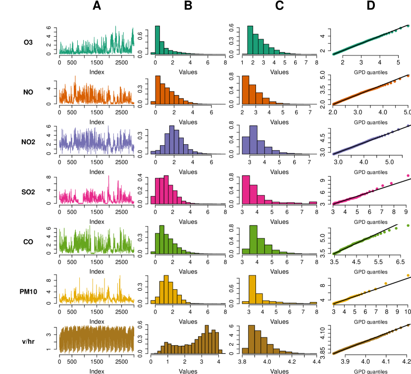
Figure 1: (A) Time series (B) Histograms (C) Histogram above extreme threshold (D) GPD Q-Q plot.

In Figure 2, autocorrelation (acf) and cross-correlation (ccf) functions with v/hr (along with corresponding partial quantities pacf and pccf) show that there is autoregressive serial dependence marginally. Pacf values are mostly insignificant after lag 1 except for v/hr where there is a negative pacf at lag 2. For all marginals except O3, ccf (resp. pccf) values are strongly positive for small lags (resp. negative at lag 2) and decrease as the lag increases until they become negative after lags 8–10. For O3, there is a large negative ccf spike around lag 10. Those observations coincide with what is suggested by information criteria (AIC/BIC) of the Markovian vine copulas (Table 2), see Section 5.2.

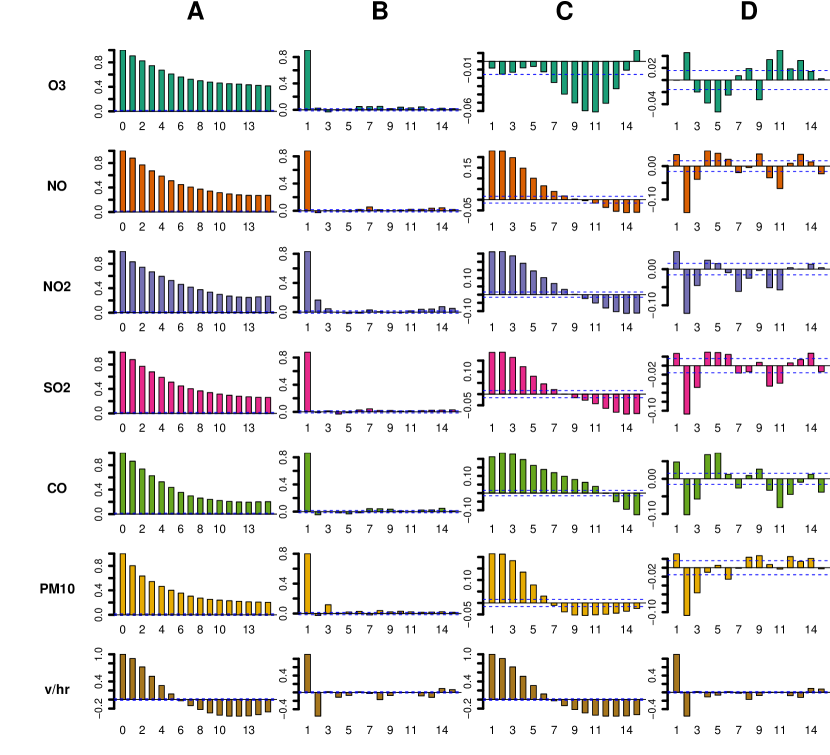
Figure 2: Correlation functions as a function of the lag difference: (A) Autocorrelation (B) Partial Autocorrelation (C) Cross-correlation with v/hr (D) Partial cross-correlation with v/hr.

	$\bm{\gamma}$	$\bm{\sigma}$	$\bm{\mu}$	$\bm{\mu}_{0}$	ADF stat.
O3	-0.191 (.010)	1.316 (.024)	1.495	80%	-19.193
NO	-0.152 (.009)	0.899 (.016)	2.023	80%	-23.746
NO2	-0.073 (.016)	0.748 (.017)	2.806	80%	-24.321
SO2	0.228 (.040)	0.751 (.040)	3.041	96%	-23.781
CO	0.032 (.027)	0.684 (.030)	3.454	96%	-26.683
PM10	0.431 (.039)	0.484 (.023)	2.981	94%	-25.398
v/hr	-0.202 (.017)	0.122 (.004)	3.842	92%	-56.342

Table 1: Unconditional GPD parameters estimates; extreme levels $\mu$ and corresponding quantile $\mu_{0}$; Augmented Dickey-Fuller (ADF) test statistic (critical value at the 1% significance level: $-3.43$). Asymptotic standard deviations are in parenthesis when available.

5.2 Vine selection

By AIC minimisation, we fit an ASVC with a Markov order of $10$ following the works of Nagler, Krüger and Min (2020) with Independence, Clayton, Gumbel, Frank & Joe pair-copulas, see Appendix D, which also coincides with the best order with respect to BIC. We conjecture that this reflects the capacity of the vine to capture the weaker cross-sectional dependencies observed at lags $8-10$.

Order	1	2	3	4	5	…	9	10	11	12
AIC	-22641	-23208	-23340	-23361	-23580	…	-23713	-23839	-23688	-23688
BIC	-21994	-22441	-22528	-22534	-22723	…	-22796	-22877	-22786	-22786
mBICV	-22151	-22394	-22036	-21295	-20401	…	-11147	-7342	-2346	3263

Table 2: Information criteria as a function of the ASVC Markov order.

On the other hand, the modified criterion $\mathrm{mBICV}$ with $\psi_{0}=0.9$ suggest an order of $2$, presumably only capturing the strong autoregressive serial dependencies suggested by the acf/pacf values (A & B, Fig. 2).

5.2.1 Synthetic data

As mentioned in Sections B & 4.4, we leverage the conditional sampling feature of the ASVC to approximate the intervention sampling mechanism. In the 20,000 samples of the dataset, a v/hr marginal extreme event occurs in $8\%\approx 1,500$ of them. Therefore, we generate $1,500$ samples of $\mathbb{X}_{t+1}(k)$ for $k=6$ given $\mathbb{X}_{t}={\bm{x}}_{t}$ such that $x^{\texttt{v/hr}}_{t}>\mu^{\texttt{v/hr}}$ where ${\bm{x}}_{t}$ is taken from the dataset. Similarly, we simulate $1,500$ samples of $\mathbb{X}_{t+1}(k)$ where $\mathbb{X}_{t}={\bm{x}}_{t}$ such that $x^{\texttt{v/hr}}_{t}\leq\mu^{\texttt{v/hr}}$ (and ${\bm{x}}_{t}$ is also from the dataset). Note that we fix the other marginals $j\neq{\texttt{v/hr}}$ to prevent instantaneous causality as given in (11).

For comparison purposes, we downsample the dataset into two sets of $1,500$ realisations of $\mathbb{X}_{t}(k)$ with/without the v/hr marginal extreme event such that $\mathbb{X}_{t}={\bm{x}}_{t}$ is the same as the one used in the conditional sampling approach mentioned above. We use those two sets to compute empirical (counter)factual probabilities and corresponding PCs at a similar level of uncertainty as with the vine-generated data.

Finally, we apply a unit Exponential marginal transformation to the data ($\gamma=0$ and $\sigma=1$) as mentioned in Section 4.6. Also, the impact threshold $v\in\mathbb{R}$ is set to the $80\%$-quantile of the unit Exponential, see Section 5.4.3 for a remark on the matter.

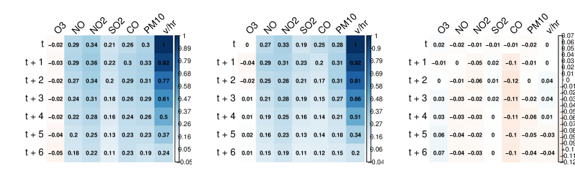
Figure 3: Componentwise correlation between $X^{\texttt{v/hr}}$ and $\mathbb{X}_{t+1}(k)$ of (left) real data; (middle) synthetic data; (right) their componentwise difference.

As pictured in Figure 3, the correlation between $X^{\texttt{v/hr}}$ and other marginals are all positive for $t+1,\dots,t+6$ except for O3 which are all not significantly non-zero. Those features are well replicated in the dataset as shown in the middle and right-hand side plots with correlation differences below $6\%$ all components across the following 6-hour window, except for CO. For that particular pollutant, correlations are underestimated in the synthetic data with error ranging from $-10\%$ to $-12\%$.

5.2.2 Uniform weights

In this section, we focus on the case of a uniform weight vector, that is, where $w_{l}=1/kd$ for $l\in\{1,\dots,kd\}$ and no component controls the likelihood of the impact event except through their factual and counterfactual distributions. We show qualitatively in Figure 4 that the synthetic data replicates the main characteristics of (counter)factual probabilities and the associated PCs as the impact threshold $v$ grows.

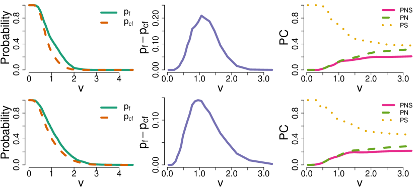
Figure 4: Probabilities with uniform weights for (top) real data and (bottom) synthetic data: (left) $p_{\mathrm{f}}$ and $p_{\mathrm{cf}}$ against the impact threshold $v$; (middle) their difference; (right) the corresponding probabilities of causation (PNS in pink bold, PN is green dashed and PS in yellow dotted lines).

The fact that $p_{\mathrm{f}}>p_{\mathrm{cf}}$ is a necessary condition for the monotonicity assumption as shown on the two left-hand side and middle plots in Fig. 4. The empirical (counter)factual probabilities showcase a wider difference $p_{\mathrm{f}}-p_{\mathrm{cf}}$ of $20\%$ for $v=1.2$ as opposed to the maximum of $15\%$ at also $v=1.2$ for the synthetic probabilities. Although the factual probabilities share similar behaviour across the different values of $v$, the synthetic counterfactual probabilities stay higher as opposed to their empirical counterparts. Both probabilities are approximately equal as $v\downarrow 0$ or as $v\uparrow\infty$. The probabilities of causation are very similar too: $\mathrm{PS}$ decreases from $100\%$ to $\approx 60\%$ as $v\rightarrow\infty$ whilst $\mathrm{PN}$ and $\mathrm{PNS}$ increase hand-in-hand from $0\%$ to approximately $\approx 40\%$. Although Kiriliouk and Naveau (2020) reported that PNS is not monotonous as a function of $v$ for simulated data but rather bell-shaped, it is increasing in our case. On the other hand, PN values are lower than those stated in the aforementioned article. We attribute those differences to the underlying structure and dependencies of the data.

5.3 Maximising the probabilities of causation

In this section, we focus on maximising the PCs with respect to the weight vector ${\bm{w}}$ (Section 4.1.1).

5.3.1 Implementation details

The optimisation is done in two stages: starting from the uniform weights, we build an initial guess in $[0,1]^{kd}$ using the differential evolution algorithm, a global optimisation routine implemented in the R package DEoptim (Mullen et al., 2011) with a number of candidates equal to ten times the dimension of ${\bm{w}}$. Next we optimise by using the L-BFGS-B scheme, potentially by adding a regularisation term as in (10) and explored in Section 5.4. We present standardised weight matrices that are computed as follows

$$\tilde{w}_{l}=\frac{w_{l}}{\max_{1\leq m\leq kd}w_{m}}\in[0,1].$$

Also, we set the threshold $v$ to be the $80$%th quantile of the unit Exponential distribution, i.e. $v\approx 1.60$.

The PNS and PS weight matrices look very similar, with high weights for v/hr for $t+1$ through $t+4$.

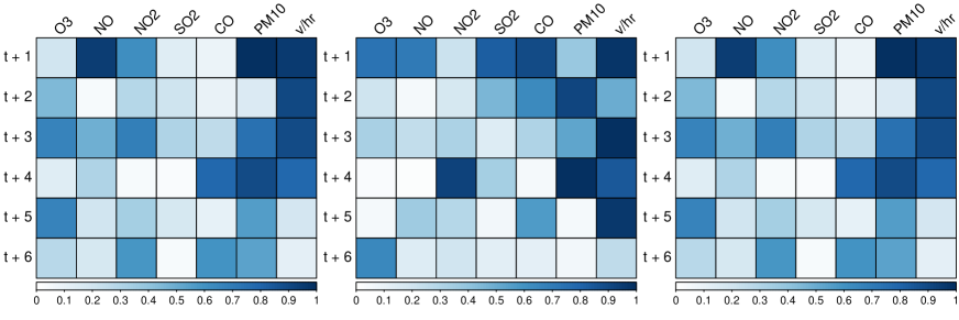
Figure 5: Weight matrices after maximisation: (left) PNS; (middle) PN; (right) PS.

At $t+1$, both the weights of NO2 and PM10 are also high which is sensible since they are related to exhaust fumes, road dust and pollen material produced or moved by cars (Coria et al., 2015, p. 180). The NO weight is also very high as it may be produced by the oxidation of NO2 (Crutzen, 1979, p. 444). We also observe mid-ranged weights at $t+3$ and $t+5$ for O3 which may come as a by-product of nitrate oxides (NO & NO2, see p. 445, Crutzen (1979)) or from volatile organic compounds, such as CO, coming from gasoline combustion, that react with ultraviolet rays (Crutzen, 1979, p. 445). We refer the interested reader to the comprehensive review in Crutzen (1979) for a detailed summary of the competing chemical reactions.

Regarding the weights related to PN, we observe that all marginals except NO2 are above $40\%$ of the maximum weight at $t+1$. CO has much higher weights than in the PNS and PS cases, with $70\%$ of the maximum at time $t+1$ and between $20\%$ and $40\%$ at times $t+2,t+3$ compared to close to $0\%$ in either the PNS or the PS case.

5.3.2 Influence of the cause marginal on the impact event

As pictured in Fig. 2, v/hr exhibits an autoregressive serial dependence which could be picked up the causal probabilities as a causal link. To verify this statement, we perform an ablation study where we remove the cause marginal (v/hr) from the impact event and observe the potential changes in the PCs and distribution of the weights.

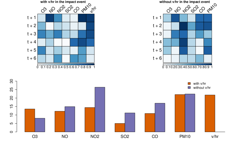
Figure 6: PNS maximisation with or without the cause marginal v/hr in the impact event. (top left) standardised weights that include v/hr; (top right) standardised weights that do not include v/hr; (bottom) contribution (in %) of each marginal in the weight vector either with v/hr or without v/hr in the impact event.

Removing v/hr changes the output substantially. In Figure 6, we plot the PNS weight matrices after maximisation with and without v/hr in the linear impact event. The bottom bar plots show the proportion of the weights attributed to each marginal separately. We can infer that most of the weight mass is transferred onto NO2 that increases from $15\%$ to more than $25\%$. The weight concentration on PM10 remains high around $20\%$, SO2 almost doubles to 12% whilst 03 is almost halved from $13\%$ down to $7\%$. See Section 5.4 for additional details on the impact of adding the cause marginal into the impact event.

5.4 Regularisation

Regularisation is a usual tool to increase the weight concentration on the most significant contributing variables. A Ridge-like regularisation ($p=2$) is equivalent to assuming a Gaussian prior on the weights. The case $p=1$ implies a Laplace prior distribution on the weights, which features a higher probability around zero than the Gaussian case. This means that more insignificant weights will most probably be set to zero.

In this section, we showcase the behaviour of the impact event weights as we increase the regularisation parameter $\lambda$ starting from the unregularised case ($\lambda=0$). We present the maximal PCs (PNS, PN, PS) obtained for different values of $\lambda$ along with the entropy of their weights, a statistic that we detail in the next section

5.4.1 Shannon’s entropy

We suppose that the sum of the weights is equal to one, i.e. $\bm{1}^{\top}{\bm{w}}=1$. To characterise the distribution of the weights, we compute the standardised Shannon’s entropy (Shannon, 1948) of the impact weights; that is, relative to the uniform weights which maximise this said entropy to obtain a value between $0$ and $1$. The statistic is given by

$$-{\bm{w}}^{\top}\log{\bm{w}}/\log(kd)\in[0,1].$$

The relative entropy is equal to one when the weights are uniformly distributed ($w_{l}=1/(kd)$ for all $l\in\{1,\dots,kd\}$); and equal to zero when the weights are concentrated on a particular component: i.e. if for some $j\in\{1,\dots,kd\}$, we have

$$w_{l}=\begin{cases}1,&\text{if $l=j$},\\ 0,&\text{if $l\neq j$}.\end{cases}$$

Between the two corner cases, the relative entropy gives some information about the concentration of the weights, from the uniformly distributed case to a deterministic distribution. We use this value to quantify the role of the regularisation term on the weight vector distribution after maximisation.

5.4.2 Results

We proceed to maximise the PNS, PN and PS with respect to ${\bm{w}}$ when v/hr is included, or not, in the impact event for an increasing regularisation parameter $\lambda\in\{0,0.001,0.01,0.1,0.5,1,5,10,100,200\}$ and $p\in\{1,2\}$. Again, the impact extreme threshold is set as the $80\%$ Exponential quantile, i.e. $v\approx 2.52$.

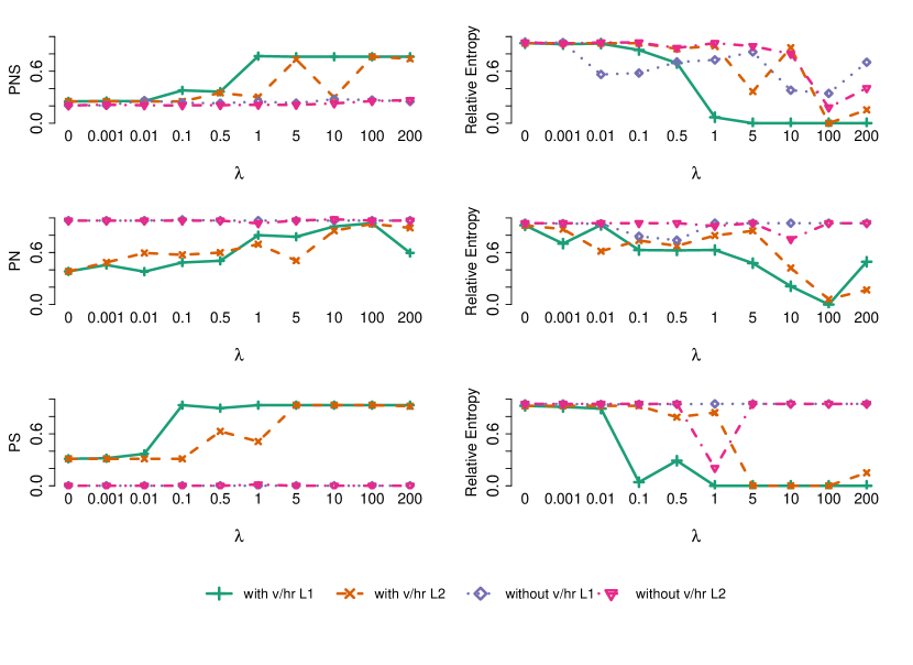
Figure 7: PC maximisation as a function of the regularisation parameter $\lambda$: (left) PNS, PN and PS values obtained, respectively. (right) entropy relative to the uniform case (lower means the weights are more concentrated) for each case;

Probabilities of causation

Figure 7 features all three cases with each row containing both the maximised PC value and the relative entropy as a function of $\lambda$. In the first row, the relative entropy of both cases with and without v/hr starts close to $1$ and decreases as $\lambda$ gets larger, down to $0$ for $\lambda\geq 5$ when v/hr is included under an $L^{1}$ penalty (i.e. $p=1$). We observe that the PNS stays relatively constant at $\approx 20\%$ across the four cases for $0\leq\lambda\leq 0.5$. Then, when v/hr is included under an $L^{1}$ penalty, as the relative entropy gets lower, the PNS surges past $95\%$ for any $\lambda\geq 1$. Similar behaviour is also obtained for the $L^{2}$ penalty, albeit decreasing sharply for $\lambda=10$. We explain this decrease by the fact that the regularisation may change the optimisation landscape in a non-linear manner. On the other hand, when v/hr is not included in the impact event, the PNS stays constant while the relative entropy decreases at about $50\%$ for all three other cases, showing that the regularisation has an effect on the weight vector although not increasing the PNS when v/hr is not included. This indicates that, as expected, v/hr brings some unique information that changes the behaviour of the PNS, similarly as it does for PS in the third row. We attribute this feature to the strong autoregressive serial dependency of v/hr.

Interestingly, we observe that when $\lambda=0$, including v/hr yields similar PN and PS values ($\approx 50\%$) as in Figure 4 for $v\approx 2.52$, meaning that the maximisation does not help much for low values of the regularisation parameter $\lambda$. However, when v/hr is excluded, the PS drops to zero whilst the PN is larger than $95\%$ for all values of $\lambda$. This suggests that an extreme in v/hr is necessary to imply extremes in some other marginals in the following six hours although not sufficient, that is, that the probability that an impact extreme would happen when an extreme in v/hr has not happened is still relatively high.

Weight matrices

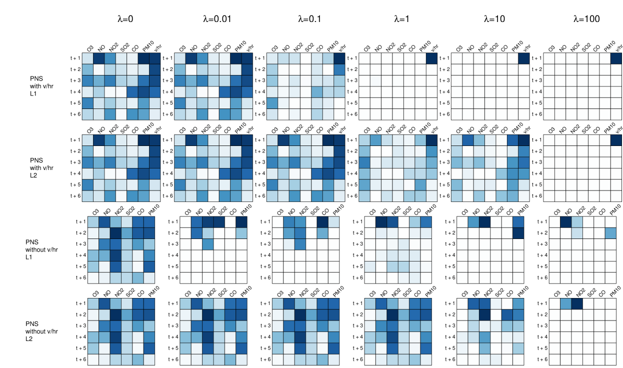
Figure 8: PNS maximisation with (top 2 rows) or without (bottom 2 rows) the cause marginal v/hr in the impact event, as a function of the regularisation parameter $\lambda\in\{0,0.01,0.1,1,10,100\}$ (from left to right) and of the norm in the regularisation term with $p=1$ on odd rows and $p=2$ on even rows.

Complementarily, we plot the standardised PNS weight matrices after maximisation in Figure 8. A first observation is that the $L^{2}$ penalty requires a much higher $\lambda$ to produce similar levels of sparsity with only the case $\lambda=100$ showcasing only a few positive weights as opposed to requiring only that $\lambda\geq 1$ for the $L^{1}$ penalty cases.

We also notice that, as mentioned above, the presence of v/hr concentrates solely the weights on v/hr at $t+1$ as shown in the two top rows. On the other hand, in the two bottom rows, removing v/hr implies a weight concentration on NO, NO2 and a bit on PM10 for $t+1$ mostly (for $\lambda=100$, i.e. last column). In addition, for $\lambda=0.1$ with the $L^{1}$ penalty or $\lambda=10$ with the $L^{2}$ penalty, the weights of NO, NO2 and PM10 are still dominant, but so are the weights of CO at $t+1$ and $t+2$ as well as $t+2$ and $t+3$, respectively. This means, on the short term, traffic spikes lead to high concentration of nitrate oxides (NOX) and of organic compounds such as CO as described in Crutzen (1979).

Note that although we presented the presence of the cause marginal (v/hr) and regularisation separately at first, their interplay is key to understand the added value of pruning weaker weights.

Finally, we observe that although both CO and SO2 have similarly (cross-)correlations with v/hr (see Fig. 3), their causal weights are very different which supports the intuition that probabilities of causation capture dependencies beyond linear relationships.

5.4.3 Discussion

The impact threshold $v\in\mathbb{R}$ is key to determine the levels above which the impact function $h$ is considered to be extreme. Choosing a large threshold implies that the number of times the impact event occurs in the dataset will thin out, highlighting the importance of tail probability approximations (Section 4.6). Also, in general, finding a threshold that is consistent for all weight vectors ${\bm{w}}$ remains an open problem when the impact event is not obtained by the application at hand (e.g. Section 5.1, Bevacqua et al. (2017)). The marginal transformation trick (Section 4.6) is a potential solution to generate quantities closed under some transformation of interest (e.g. weighted sum).

Sparse impact events are obtained as the regularisation term ramps up, with only certain links appearing as significant in this context. However, we see that the strong positive autocorrelation in v/hr leads to high impact weights, not necessarily solely from causal relationships. Although we mention that vine copulas can form a sparse dependence structure, dedicated sparse structures for extremes (Engelke and Ivanovs, 2021) offer theoretical guarantees that they retrieve the true tree-based description of true extremal dependencies under the assumptions that those relationships are static in time and unconditioned (outside the counterfactual theory). On the contrary, vine copulas can capture dependencies in a flexible and scalable manner through time and cross-sections but are only equipped with their tail dependence function (may they exist) to quantify their extremal behaviour. Although we presented the theoretical foundations of copulas and their practical implications when it comes to tail modelling (Section 3), an investigation in the spirit of Engelke and Volgushev (2019) for vine copulas, linking the information criteria with the extremal structure hence created, remains unexplored to our knowledge. Although this goes beyond the scope of this article, a first step could be to maintain a collection of structures that capture separately factual and counterfactual relationships as mentioned in Section4.1.2 and this work is the first step in this direction—at least empirically.

6 Conclusion

6.1 Summary

In this article, we introduce the Extreme Event Propagation (EEP) framework which deals with the temporal and cross-sectional propagation of a cause extreme event on an impact event. We quantify their relationship through a counterfactual framework (Pearl, 1999), equipped with a set of three probabilities of causation where we compare two versions of the world: one where the cause has happened and one where it has not. By doing so, we obtain some information about the ”cause” extreme event triggering the impact event at a later time.

Although the EEP framework is model-agnostic, we explore different properties of multivariate peaks-over-thresholds distributions such as extremal correlations, regularly varying distributions and tail dependence functions that we believe are essential to represent accurately the extremal structure between different time series. We then select a copula-based approach that satisfies most of those properties; where marginals have generalised Pareto-distributed upper tails and are linked together through a stationary and flexible dependence structure, namely using stationary Archimedean vine copulas (Nagler, Krüger and Min, 2020).

We focus on marginal extreme events as the cause of a linear impact extreme event (Kiriliouk et al., 2019) for interpretability purposes. By maximising those said probabilities of causation with respect to the linear projection weight, we obtain which and when are the probable marginals to become extreme. Regularisation in the form of an $L^{1}$ or $L^{2}$ penalty is also explored to help extract the most significant causal links. This said, our analysis is applicable to settings where the impact event is fully characterised (Bevacqua et al., 2017) or beyond the linear case.

Finally, we apply the EEP framework to an air pollution dataset to study the impact of high road traffic on air pollutant concentration. We retrieve the chemical and physical reactions documented in the literature (Crutzen, 1979; Coria et al., 2015) and observe that regularising the problem helps in generating interpretable (e.g. sparse) results about the underlying causal dynamics.

6.2 Outlook

Studying the propagation of extremes through a causal framework poses a number of challenges. Understanding which variables are the most probable to become extreme themselves is currently estimated in two ways: by inspection of the weights or via regularisation. However, devising a hypothesis testing framework or a theoretical understanding of the induced regularisation bias, respectively, to quantify the weight significance remain open problems. By including serial and cross-sectional dependencies at the heart of the EEP framework using stationary vine copulas, we contribute to forming a family of approaches in addition to the current static methods (Hannart and Naveau, 2018; Kiriliouk et al., 2019; Mhalla, Chavez-Demoulin and Dupuis, 2020). Given the similarity between our modelling framework and recent contributions regarding extreme values through sparse structures (Engelke and Volgushev, 2019; Engelke and Ivanovs, 2021), we believe that a formal link between those approaches is bound to be exploited in the near future.

Appendix A Baseline bivariate copulas or pair-copulas

We apply a stationary Markovian vine model with Archimedean or independent bivariate copulas. This allows capturing tail dependence across the marginals themselves. We control the fitting performance and the number of parameters included in this second layer using information criteria such as AIC, BIC or sparse modified BIC for vines (mBICV) (Nagler, Bumann and Czado, 2018).

A key limitation of traditional copulas is the incapacity to scale up with the number of variables since those copulas are often parametrised with very few parameters (one or two).

Regular vine construction of copulas is performed using a constellation of parametric bivariate dependence functions (Grothe and Nicklas, 2013), see Definition 13, which we call pair-copulas. The regular vines pair construction is detailed in Section 4.3.1. Since copulas are designed to capture dependency, a common measure of dependence is Kendall’s $\tau$ (Embrechts, Klüppelberg and Mikosch, 2013).

Name	Copula $C({\bm{u}};\theta)$	Generator $\phi(t,\theta)$	Parameter $\theta$
Independence	$\prod_{i=1}^{d}u^{i}$	$e^{-t}$	$\emptyset$
Clayton	$\left(\sum_{i=1}^{d}(u^{i})^{-\theta}-(d-1)\right)^{-1/\theta}_{+}$	$\theta^{-1}(t^{-\theta}-1)$	$\theta\in[-1,\infty)\char 92\relax\{0\}$
Gumbel	$\exp\left\{-\left\{\sum_{i=1}^{d}(-\ln u^{i})^{\theta}\right\}^{-1/\theta}\right\}$	$(-\ln t)^{\theta}$	$\theta\in[1,\infty)$
Frank	$-\theta^{-1}\ln\left(1+\frac{\prod_{i=1}^{d}\left(e^{-\theta u_{i}}-1\right)}{(e^{-\theta}-1)^{d-1}}\right)$	$-\ln\frac{e^{-\theta t}-1}{e^{-\theta}-1}$	$\theta\in\mathbb{R}\char 92\relax\{0\}$
Joe	$1-\left[\sum_{i=1}^{d}(1-u_{i})^{\theta}-\prod_{i=1}^{d}(1-u_{i})^{\theta}\right]^{-1/\theta}$	$-\ln(1-(1-t)^{\theta})$	$\theta\in[1,\infty)$

Table 3: List of the four Archimedean pair-copulas.

Remark 4.

To obtain negative dependence between variables, there are rotated copulas to capture better positive and negative dependency: to do so, we use the transformation $u\mapsto 1-u$ on either one or both variables to rotate the scatter plot and fall back to the case where $\tau>0$.

The first author was supported by EPSRC grant number EP/R014604/1. AV would also like to acknowledge funding by the Simons Foundation.

We present a short overview of the different notions of time series causality in Appendix B. Core definitions from the counterfactual causal theory of Pearl (1999) that we use the EEP framework are presented in Appendix C. Finally, we recall the vine copula definitions and concepts that we leverage in Appendix D.

Appendix B Time series causality

We present a short overview of different causality notions for time series.

B.1 General context

Understanding causality in the context of time series analysis is often based on the celebrated Granger causality (Granger, 1980, 1988) which can be applied and tested in many time series models from autoregressive models (Granger, 1980, Section 5) to copulas (Kim, Lee and Hwang, 2020) but can capture the spurious causal links in the presence of confounding (latent) variables (Eichler, 2013, Section 4). Granger causality is often compared to Sims causality (Sims, 1972; Florens and Mouchart, 1982), structural causality (White and Lu, 2010) and intervention causality (Eichler and Didelez, 2007); the EEP framework is most closely related to the two last items. We refer to Eichler (2013) for an insightful discussion and comparison of the four causality frameworks.

B.2 Interventions and causality

Two usual assumptions regarding time-series causality are that (a) the cause precedes its effects in time; and, (b) manipulations of the cause change the effects (Eichler, 2013, Section 2.c.), as defined for the celebrated Granger causality (Granger, 1980, 1988). Intervention causality (Eichler, 2013, Section 2.b.) is defined for four different intervention regimes (e.g. idle, atomic, conditional & random) dictating the behaviour of the (non-random) intervention indicator $\zeta^{i}_{t}$ which gives information about how the data is generated or observed (Eichler and Didelez, 2007, Def. 2.1 & Rem. 2.2).

In theory, in the EEP framework, we would focus on either the random regime where the conditional distribution of $\mathbb{X}_{t+1}(k)$ given $\mathbb{X}_{0}(t)$ is known; or the conditional regime, where $\mathbb{X}_{t+1}(k)$ is forced to take a value that depends on past observations of $\mathbb{X}_{0}(t)$. However, as it often impractical or not feasible to collect data under the interventional regime, we work under the idle regime which coincides with the observational regime, where $\mathbb{X}$ arises naturally, to model dependencies and leverage this structure to generate data under intervention.

We approximate the conditional intervention regime by leveraging the conditional sampling capabilities of vine copulas, see Section 4.4. More precisely, we borrow elements from the structural causality framework (White and Lu, 2010) which states that the data is generated according a recursive dynamic structure. For a cause of interest $X_{t}$, an impact of interest $Y_{t}$ and a collection of (additional) observed variables $Z_{t}$ and unobserved ones $U_{X,t},U_{Y,t}$, where $t\in\mathbb{N}$, we have:

$$X_{t+1}=q_{x,t}\left(X_{0}(t),Y_{0}(t),Z_{0}(t),U_{X=x,t+1}\right),\quad\text{and}\quad Y_{t+1}=q_{y,t}\left(X_{0}(t),Y_{0}(t),Z_{0}(t),U_{Y=y,t+1}\right),$$

for an unknown function $q_{\cdot,t}$. This dependence structure resembles that of vine copulas (Joe, Li and Nikoloulopoulos, 2010; Bedford and Cooke, 2002, 2001) especially when tailored for time series (Nagler, Krüger and Min, 2020; Smith, 2015; Beare and Seo, 2015; Brechmann, Czado and Aas, 2012), under the assumption that there are no unobserved variables.

This collection of links between causality structures and vine copulas explains why they are strong modelling candidates; in addition, we recall the theoretical guarantees and properties of vine copulas for multivariate extreme value modelling in Section 3. A key component in counterfactual causality modelling is the methodology used to compare different settings, which we discuss in the following section.

B.3 An alternative measure of causality

As opposed to using probabilities of causation, causality in the context of time series is usually quantified using the average causal effect ($\mathrm{ACE}$) (Eichler, 2013, Def. 2.1). Informally, it unveils the impact of the intervention at time $t$ in the sense of an exceedance in expectations between the target variable at time $t+h$ under intervention and without it. It is defined by

$$\mathrm{ACE}^{(i,j)}_{x}(h)\overset{\Delta}{=}\mathbb{E}(X^{j}_{t+h}\ |\ do(X^{i}_{t}=x))-\mathbb{E}(X^{j}_{t+h}),\quad\text{for $x\in\mathbb{R}^{d}$, $i,j\in I$ and $h\in\mathbb{N}$},$$

where the expectation is taken under the observed probability measure P without interventions as mentioned above. In this setting, Eichler and Didelez (2007) discusses causality identifiability: under the conditional or random regimes, if $i,j\in S\subseteq I$ then $S$ identifies the effect of $X^{i}_{t}$ on $X^{j}_{t+h}$ for all $h\in\mathbb{N}$ if an intervention in $X^{i}_{t}$ with intervention indicator $\zeta^{i}_{t}$ satisfies

$$\{\mathbb{X}_{0}(t-1),\ (X^{j}_{t},\ j\neq i)\}\perp\!\!\!\perp\zeta^{i}_{t},\quad\{\mathbb{X}_{t+h},\ h\in\mathbb{N}\}\perp\!\!\!\perp\zeta^{i}_{t}\ |\ \mathbb{X}_{0}(t),\quad\text{and}\quad X^{j}_{t+h}\perp\!\!\!\perp\zeta^{i}_{t}\ |\ \mathbb{X}_{0}(t),$$ (11)

for all $h\in\mathbb{N}$, with the (conditional) independence ($\perp\!\!\!\perp$) from Dawid (1979), see below. The first assumption ensures that intervening on the past or any other variables at time $t$ which excludes instantaneous causality. The second independence means that the future values are only affected by interventions through past variables; similarly, the third assumption states that the target variables are only affected by interventions through past variables.

By considering the difference between factual and counterfactual interventions, the ACE can extend the concept of the PNS beyond (and including) binary events. However, the PCs quantify in three different ways the relationship of the cause on the impact events which we believe are better suited to reflect the complex mechanisms involved in the propagation of extremes. That is, they gain value when presented jointly (see Section 5). Sufficient and necessary causations are thought to be complementary: on page 95, Pearl (1999), it is explained that

$[...]$ necessary causation is a concept tailored to a specific event under consideration, while sufficient causation is based on the general tendency of certain event types to produce other event types. Adequate explanations should respect both aspects. If we base explanations solely on generic tendencies (i.e., sufficient causation), we lose important specific information. [emphasis in original]

Note that, in this context, the independence $X\perp\!\!\!\perp Y$ holds if and only if $f_{X,Y}=\tilde{f}_{X}\times\tilde{f}_{Y}$ where $\tilde{f}_{X},\tilde{f}_{Y}$ are not necessarily the marginal densities $f_{X},f_{Y}$. Similarly, $X\perp\!\!\!\perp Y|Z$ if and only if $f_{X,Y|Z}=\tilde{f}_{X|Z}\times\tilde{f}_{Y|Z}$ where $\tilde{f}_{\cdot|Z}$ are proper distributions. This highlights the fact that any marginal distributions does not depend on the other marginal distributions. Also, $X^{j}_{t+h}\perp\!\!\!\perp\zeta^{i}_{t}$ for some $h\in\mathbb{N}$ means that the distribution of $X^{j}_{t+h}$ is the same under any of the intervention regimes.

Appendix C Primer on the counterfactual causal theory

C.1 Causal models, actions and potential response

Causality requires to separate internal variables of the system under study from external ones as well as the knowledge of how they are related to one another, as formalised in the following definition:

Definition 2.

(Pearl, 1999, adapted from Def. 1) A causal model is a triple $M=(U,V,F)$ where

1. $U$ is a set of variables called exogenous that are determined by factors outside the model.

2. $V=\{V_{1},\dots,V_{d}\}$ is a set of variables, called endogenous, that are determined by variables in the model, namely, by variables in $U\cup V$.

3. $F=\{f_{1},\dots,f_{d}\}$ where each $f_{i}:U\times(V\char 92\relax V_{i})\rightarrow V_{i}$ gives the value of $V_{i}$ given the values of all other variables in $U\cup V$ which can be represented by

   $$v_{i}=f_{i}(pa_{i},u_{i}),\quad i\in I,$$

   where $pa_{i}$ (resp. $u_{i}$) is any realisation of the unique minimal set of parent variables $\mathrm{PA}_{i}$ (resp. $U_{i}$) in $V\char 92\relax V_{i}$ (resp. in $U$) that renders $f_{i}$ nontrivial.

Note that the definition of endogenous variables is recursive and they are fully determined by exogenous variables. A causal model $M$ is commonly associated with a directed graph called the causal graph and denoted $G(M)$, where $V$ are the nodes and the directed edges are from the parent variables in $\mathrm{PA}_{i}$ towards $V_{i}$ for any $i\in I$.

Definition 3.

(Pearl, 1999, Def. 2) Let $M$ be a causal model and $X\subseteq V$, and $x$ be a realisation of $X$. A submodel $M_{x}$ of $M$ is the causal model $M_{x}=(U,V,F_{x})$, where $F_{x}\overset{\Delta}{=}\{f_{i}:V_{i}\not\in X\}\cup\{X=x\}$.

A submodel $M_{x}$ is similar to $M$ where all functions $f_{i}$ corresponding to variables in $X$ are replaced by constant functions such that $X=x$. Analogously, acting on $M$ by imposing $X=x$ is defined as follows:

Definition 4.

(Pearl, 1999, adapted from Def. 3) Let $M=(U,V,F)$ be a causal model, $X\subseteq V$ and $x$ be a realisation of $X$. We define the action $do(X=x)$ as the minimal change in $M$ required to make $X=x$ hold true under any $u\in U$. The effect of action $do(X=x)$ on $M$ is given by the submodel $M_{x}$.

Figure 9: Intervention $do(V_{B}=v_{B})$ on $U=\{U_{A},U_{B},U_{C},U_{D}\}$ and $V=\{V_{A},V_{B},V_{C},V_{D}\}$.

Given the effect of action $do(X=x)$, we recall the definition of the potential response

Definition 5.

(Pearl, 1999, Def. 4 & 5) Let $Y\in V$, and let $X\subseteq V$. The potential response of $Y$ in unit $u$ to action $do(X=x)$, denoted $Y_{x}(u)$, is the solution for $Y$ of the set of equations $F_{x}$. The counterfactual sentence ”the value that $Y$ would have obtained, had $X$ been $x$.” is interpreted as denoting the potential response $Y_{x}(u)$.

Furthermore, we consider the extension to probabilistic causal models defined as follows

Definition 6.

(Pearl, 1999, Def. 6) A probabilistic causal model is a pair $(M,{\text{P}}(u))$, where $M$ is a causal model and ${\text{P}}(u)$ is a probability function defined on the domain of $U$.

From Def. 2, all endogenous variables $V$ are functions of exogenous variables $U$. In that sense, for any $Y\subseteq V$, we write

$${\text{P}}(Y=y)=\sum_{u:\ Y(u)=y}P(u),\quad\text{and}\quad{\text{P}}(Y_{x}=y)=\sum_{u:\ Y_{x}(u)=y}{\text{P}}(u),$$

and similarly for all probabilities involving variables in $V$.

Notation 7.

We write ${\text{P}}\left(Y\ |\ do(X=x)\right)$ for ${\text{P}}\left(Y_{x}\right)$ to emphasise the action applied on $Y$.

C.2 Probabilities of causation

Given the definition of causal models and counterfactuals, we define three probabilities of causation ($\mathrm{PC}$) (Pearl, 1999; Hannart et al., 2016; Hannart and Naveau, 2018) which outline different relationships between some action on a causal model and its corresponding response.

Definition 8.

(Pearl, 1999, Def. 7, 8 & 9) Let $X$ and $Y$ be two binary variables in a causal model $M$. The probabilities of necessary, sufficient and necessary and sufficient causation are defined as the expressions

$$\mathrm{PN} \overset{\Delta}{=}{\text{P}}\left(Y=0\ |\ do(X=0),\ X=1,\ Y=1\right),\quad$$ (necessary),

$$\mathrm{PS} \overset{\Delta}{=}{\text{P}}\left(Y=1\ |\ do(X=1),\ X=0,\ Y=0\right),\quad$$ (sufficient),

$$\mathrm{PNS} \overset{\Delta}{=}{\text{P}}\left(\left\{Y=0\ |\ do(X=0)\right\}\cap\left\{Y=1\ |\ do(X=1)\right\}\right),\quad$$ (necessary and sufficient).

We note that the PC quantities are linked through the relationship (Pearl, 1999, Lemma 1)

$$\mathrm{PNS}={\text{P}}(X=1,Y=1)\cdot\mathrm{PN}+P(X=0,Y=0)\cdot\mathrm{PS}.$$

Necessary causation ($\mathrm{PN}$) is defined as the likelihood that $Y$ would be zero had $X$ been $0$, given that, in reality both $Y$ and $X$ are actually $1$. Sufficient causation $(\mathrm{PS})$ is the opposite: it is the likelihood that $Y$ would be $1$ had $X$ been $1$, when both $X$ and $Y$ are actually equal to $0$. The probability of necessary and sufficient causation ($\mathrm{PNS}$) sits in between as the likelihood that $Y$ is equal to $1$ had $X$ been $1$ and that $Y$ is $0$ had $X$ been equal to $0$. We translate those probabilities into the EEP framework in Section 2.5. Those probabilities can be defined on a causal model $M$ which can or cannot be identifiable in the following sense:

Definition 9.

(Pearl, 1999, Def. 12) Let $Q(M)$ be any quantity defined on a probabilistic causal model $(M,{\text{P}})$. $Q$ is identifiable in a class ${\mathcal{M}}$ of causal models if and only if any two models $(M_{1},{\text{P}}_{M_{1}}),(M_{2},{\text{P}}_{M_{2}})\in{\mathcal{M}}$ that satisfy ${\text{P}}_{M_{1}}={\text{P}}_{M_{2}}$ also satisfy $Q(M_{1})=Q(M_{2})$. In other words, $Q$ is identifiable if it can be determined uniquely from the probability distribution P of the endogenous variables $V$.

Notation 10.

Let $x$ stand for $\{X=1\}$ and, $x^{c}$ for its complement $\{X=0\}$.

To ensure the identifiability of all three $\mathrm{PC}$, it is usual to assume the exogeneity and monotonity of $X$ with respect to $Y$ (Pearl, 1999, Section 3.3) which we recall below:

Definition 11.

(Pearl, 1999, Def. 13) A variable $X$ is said to be exogenous relative to $Y$ in a causal model $M$ if and only if (iff) ${\text{P}}(Y_{x}=1,\ Y_{x^{c}}=1\ |\ x)={\text{P}}(Y_{x}=1,\ Y_{x^{c}}=0)$, i.e. iff the potential response of $Y$ to the action $x$ or $x^{c}$ is independent of the actual value of $X$.

A key property of exogeneity is the identification of ${\text{P}}(Y|do(X))$ to the corresponding conditional probability ${\text{P}}(Y|X)$ which allows for computation using empirical data, see Section B.

Definition 12.

(Pearl, 1999, Def. 14) A variable $Y$ is said to be monotonic relative to variable $X$ in a causal model $M$ iff the junction $Y_{x}(u)$ is monotonic in $x$ for all realisation $u$ of $U$. Equivalently, $Y$ is monotonic relative to $X$ iff ${\text{P}}(Y_{x}=0,\ Y_{x^{c}}=1)=0$.

That is, if $Y$ is monotonic relative to $X$, then $Y$ can only move in the same direction as $X$: a condition change from $x^{c}$ to $x$ (i.e. $X$ grows from 0 to 1) will not change $Y$ from $y$ to $y^{c}$,i.e. decreases from $1$ to $0$, irrespective of the exogenous variables. Under both exogeneity and monotonity conditions, all three $\mathrm{PC}$ are identifiable (Pearl, 1999, Th. 3).

Appendix D Archimedean Stationary Vine Copulas

We call Archimedean stationary vine copulas (ASVC) any stationary vine copulas constructed using either Archimedean or independent bivariate copulas which act as building blocks and propagate dependencies through the vine trees.

D.1 Definitions

We define a tree $T=(N,E)$ as an acyclic graph, where $N$ is its set of nodes and $E$ is its set of edges (unordered pairs of nodes), see Def. 4, Bedford and Cooke (2001).

D.1.1 Vine copulas

We recall the definitions of vines and regular vine copulas (or R-Vine):

Definition 13.

(Bedford and Cooke, 2001, Def. 8) A vine ${\mathcal{V}}$ on $d$ elements is an ordered sequence of trees $\mathcal{T}\overset{\Delta}{=}(T_{1},\dots,T_{m})$ with $T_{l}\overset{\Delta}{=}(N_{l},\ E_{l}),$ for $l\in\{1,\dots,m\}$ such that:

1. $N_{1}\overset{\Delta}{=}\{1,\dots,d\}$ i.e. the first tree has nodes 1,…,d;

2. for $l\geq 2$, $T_{l}$ is a tree with nodes $N_{l}\subset N_{1}\cup E_{1}\cup\dots\cup E_{l-1}$.

A vine ${\mathcal{V}}$ is a regular vine on $d$ elements if

1. it is made exactly $d$ trees, i.e. $m$ = $d$;

2. $T_{l}$ is a connected tree with a node set equal to the edge set of the previous tree, i.e. $N_{l}\overset{\Delta}{=}E_{l-1}$ with $\mathrm{card}(N_{l})=d-i+1$ for $d\in I$, where $\mathrm{card}(N_{l})$ is the cardinality of the set $N_{l}$;

3. the proximity condition holds: for $l\in\{1,\dots,d-1\}$, if two nodes from $N_{l+1}$ are connected in $T_{l+1}$, the corresponding edges in $T_{l}$ have exactly one common node.

In theory, each pair copula of the vine is fitted conditional on the uniform bivariate distribution of the previous level. However, it is usual in the literature to make the assumption that we only fit given the uniform univariate marginals themselves to make the computation more tractable.

If the trees $T_{i}$ correspond to a path (i.e. where each node has either one or two neighbours), the vine is called a D-vine. On the other hand, if the trees are stars (i.e. all but one nodes have the same unique neighbour), it is a C-vine.

Figure 10: The first tree ($T_{1}$) of a (left) D-vine; (right) C-vine on variables $\{X_{1},X_{2},X_{3},X_{4},X_{5}\}$.

D.1.2 Vine copulas for stationary multivariate time series

General context

Constraining further those tree structures generates suitable vines to model stationary multivariate time series, e.g. D-vines of Smith (2015), M-Vines of Beare and Seo (2015) and S-Vines (or stationary vines) of Nagler, Krüger and Min (2020). For simplicity, we only consider the latter in this article.

Figure 11: The first tree ($T_{1}$) of a Markov stationary vine with order $3$ on $\{X^{1}_{t},X^{2}_{t},X^{3}_{t},X^{4}_{t},X^{5}_{t}\}$ with cross-sections modelled using a D-vine.

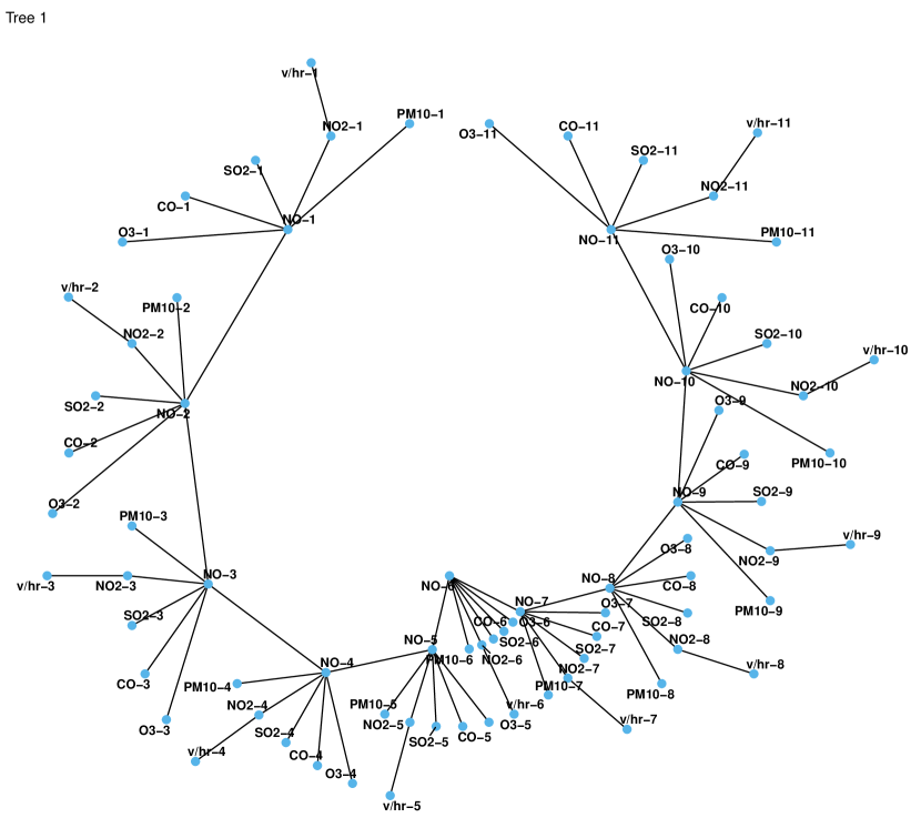
Figure 12: First tree of the stationary vine copula fitted on the air pollution dataset where the name of each variable is followed by their time horizon: O3-3 is the third value of Ozone in each 11-long data block.

All those models leverage a single vine that captures the cross-sectional dependence structure of $\mathbb{X}_{t}$ at all time points. Then, the first trees of those cross-sectional vines at time $t$ and $t+1$ are linked through a collection of edges with a vertex from the structure at time $t$ and one at time $t+1$, such that those edges are time-invariant. We consider stationary vines in this article where the cross-sectional structure is an arbitrary R-vine and the vine copula model is translation invariant (Nagler, Krüger and Min, 2020, Def. 4). For instance, in Figure 12, we observe that along the backbone $\text{NO-1},\dots,\text{NO-11}$, the cross-sectional vine structure remains the same similar to the D-vine in Fig. 11.

Definitions

We introduce the main definitions necessary for the definition of stationary vine copulas. The interested reader might find it useful to consult Section 2, Nagler, Krüger and Min (2020) for a comprehensive description of stationary vine copulas.

Recall that a vine copula model associates each edge of an regular vine with a bivariate copula. We write $({\mathcal{V}},{\mathcal{C}}({\mathcal{V}}))$ the vine structure ${\mathcal{V}}=\{(N_{l},E_{l}),\ l\in\{1,\dots,m\}\}$ and associated collection of bivariate copulas ${\mathcal{C}}({\mathcal{V}})\overset{\Delta}{=}\{c_{e}:e\in E_{k},k\in\{1,\dots,d-1\}\}$ where $d$ is the number of variables.

Definition 14.

(Nagler, Krüger and Min, 2020, Def. 4) A vine copula model $({\mathcal{V}},{\mathcal{C}}({\mathcal{V}}))$ on the set $N_{1}=\{1,\dots,N\}\times\{1,\dots,d\}$ is called translation invariant if it holds that

$$c_{a_{e},b_{e}|D_{e}}=c_{a_{e^{\prime}},b_{e^{\prime}}|D_{e^{\prime}}},$$

for all edges $e,e^{\prime}\in\in_{k=1}^{nd-1}E_{k}$ for which there is a $\tau\in\mathbb{Z}$ such that

$$a_{e}=a_{e^{\prime}}+(\tau,0),\quad b_{e}=b_{e^{\prime}}+(\tau,0),\quad D_{e}=D_{e^{\prime}}+(\tau,0),$$

where the last equality is short for $D_{e}=\{v+(\tau,0):v\in D_{e^{\prime}}\}$.

This definition is the equivalent of the strong stationary condition for vine copulas. The restriction and translation of vines relate to the translation invariance and we recall their definition:

Definition 15.

(Nagler, Krüger and Min, 2020, Def. 5) Let $({\mathcal{V}},{\mathcal{C}}({\mathcal{V}}))$ be a vine on $\{1,\dots,N\}\times\{1,\dots,d\}$ and let $N_{t}^{\prime}=\{t,\dots,t+m\}\times\{1,\dots,d\}$ for some $t,m$ such that $1\leq t\leq N$ and $0\leq m\leq N-t$. For all $k\geq 1$, define $E_{k}^{\prime}\overset{\Delta}{=}E_{k}\cap{{N_{k}^{\prime}}\choose{2}}$ and $V_{k}^{\prime}\overset{\Delta}{=}E_{k}^{\prime}$. Then the sequence of graphs ${\mathcal{V}}_{t,t+m}\overset{\Delta}{=}\{(N_{k}^{\prime},E_{k}^{\prime}):k\in\{1,\dots,(m+1)d-1\}\}$ is called restriction of ${\mathcal{V}}$ on the time points $t,\dots,t+m$.

Definition 16.

(Nagler, Krüger and Min, 2020, Def. 6) Let $m\geq 0$, ${\mathcal{V}}_{t,t+m}=\{(N_{k}^{\prime},E_{k}^{\prime}):k\in\{1,\dots,(m+1)d-1\}\}$ to be a vine on $\{t,\dots,t+\tau\}\times\{1,\dots,d\}$ and ${\mathcal{V}}_{s,s+m}$ a vine on $\{s,\dots,s+\tau\}\times\{1,\dots,d\}$. We say that ${\mathcal{V}}_{t}$ is a translation of ${\mathcal{V}}_{s}$ (denoted by ${\mathcal{V}}_{t}\sim{\bm{V}}_{s}$) if for all $k\in\{1,\dots,d-1\}$ and edges $e\in E_{t,k}$, there is an edge $e^{\prime}\in E_{s,k}$ such that $e=e^{\prime}+(t-s,0)$ (and vice versa).

Then, the stationary vines are defined through a characterisation given by the following theorem

Theorem 17.

(Nagler, Krüger and Min, 2020, Th. 1) Let ${\mathcal{V}}$ be a vine on the set $\{1,\dots,n\}\times\{1,\dots,d\}$. Then, the following statements are equivalent:

1. The vine copula model $({\mathcal{V}},{\mathcal{C}}({\mathcal{V}}))$ is stationary for all translation invariant choices of ${\mathcal{C}}({\mathcal{V}}))$.

2. There are vines ${\mathcal{V}}^{(m)}$, $m=1,\dots,n-1$, defined on $\{1,\dots,m+1\}\times\{1,\dots,d\}$, such that for all $m=0,\dots,n-1$, and $1\leq t\leq n-m$, we have

   $${\mathcal{V}}_{t,t+m}\sim{\mathcal{V}}^{(m)}.$$

Stationary vine copulas are all vine copulas that satisfy Th. 17, (ii) as it describes the notion of strong stationarity for graphs:

Definition 18.

A vine ${\mathcal{V}}$ on the set $\{1,\dots,N\}\times\{1,\dots,d\}$ is called stationarity if it statisfies condition (ii), Th. 17.

D.2 Existence and uniqueness of vine copulas

A vine copula can be seen as a proper hierarchical copula as it boils down to the existence and uniqueness of a bivariate copula (Sklar, 1959) as explained in Section 4.2, Czado (2010). The vine copulas made of given bivariate copula families provide a multi-parameter augmented coverage of a subspace of $d$-dimensional copulas of the given families. As a special case of Archimedean copulas, we quote Section 4.2.2, Czado (2010):

This construction of multivariate distributions and copulas is very general and flexible since we can use any bivariate copula as a building block in the pair-copula construction model. In contrast to the extended multivariate Archimedean copulas no restriction to the Archimedean pair-copulas or further parameter restrictions are necessary.

Vines are fitted using uniform margins and we take a semiparametric transformation approach using an empirical distribution function below the extreme thresholds $(\mu^{i},\ i\in I)$ and the asymptotic GPD above this said threshold (Coles and Tawn, 1991). Another possibility is to use the empirical distribution function throughout; see Shih and Louis (1995) for a comparison study.

References

- Allen (2003) {barticle}[author] \bauthor\bsnmAllen, \bfnmMyles\binitsM. (\byear2003). \btitleLiability for climate change. \bjournalNature \bvolume421 \bpages891–892. \endbibitem
- Angélil et al. (2017) {barticle}[author] \bauthor\bsnmAngélil, \bfnmOliver\binitsO., \bauthor\bsnmStone, \bfnmDáithí\binitsD., \bauthor\bsnmWehner, \bfnmMichael\binitsM., \bauthor\bsnmPaciorek, \bfnmChristopher J\binitsC. J., \bauthor\bsnmKrishnan, \bfnmHarinarayan\binitsH. and \bauthor\bsnmCollins, \bfnmWilliam\binitsW. (\byear2017). \btitleAn independent assessment of anthropogenic attribution statements for recent extreme temperature and rainfall events. \bjournalJournal of Climate \bvolume30 \bpages5–16. \endbibitem
- Aulbach, Falk and Fuller (2019) {barticle}[author] \bauthor\bsnmAulbach, \bfnmStefan\binitsS., \bauthor\bsnmFalk, \bfnmMichael\binitsM. and \bauthor\bsnmFuller, \bfnmTimo\binitsT. (\byear2019). \btitleTesting for a -neighborhood of a generalized Pareto copula. \bjournalAnnals of the Institute of Statistical Mathematics \bvolume71 \bpages599–626. \bdoi10.1007/s10463-018-0657-x \endbibitem
- Bacro et al. (2020) {barticle}[author] \bauthor\bsnmBacro, \bfnmJean-Noël\binitsJ.-N., \bauthor\bsnmGaetan, \bfnmCarlo\binitsC., \bauthor\bsnmOpitz, \bfnmThomas\binitsT. and \bauthor\bsnmToulemonde, \bfnmGwladys\binitsG. (\byear2020). \btitleHierarchical Space-Time Modeling of Asymptotically Independent Exceedances With an Application to Precipitation Data. \bjournalJournal of the American Statistical Association \bvolume115 \bpages555-569. \bdoi10.1080/01621459.2019.1617152 \endbibitem
- Bader and Yan (2020) {bmanual}[author] \bauthor\bsnmBader, \bfnmBrian\binitsB. and \bauthor\bsnmYan, \bfnmJun\binitsJ. (\byear2020). \btitleeva: Extreme Value Analysis with Goodness-of-Fit Testing \bnoteR package version 0.2.6 available on CRAN. \endbibitem
- Bader et al. (2018) {barticle}[author] \bauthor\bsnmBader, \bfnmBrian\binitsB., \bauthor\bsnmYan, \bfnmJun\binitsJ., \bauthor\bsnmZhang, \bfnmXuebin\binitsX. \betalet al. (\byear2018). \btitleAutomated threshold selection for extreme value analysis via ordered goodness-of-fit tests with adjustment for false discovery rate. \bjournalThe Annals of Applied Statistics \bvolume12 \bpages310–329. \endbibitem
- Balkema and De Haan (1974) {barticle}[author] \bauthor\bsnmBalkema, \bfnmAugust A\binitsA. A. and \bauthor\bsnmDe Haan, \bfnmLaurens\binitsL. (\byear1974). \btitleResidual life time at great age. \bjournalThe Annals of probability \bpages792–804. \endbibitem
- Basrak, Davis and Mikosch (2002) {barticle}[author] \bauthor\bsnmBasrak, \bfnmBojan\binitsB., \bauthor\bsnmDavis, \bfnmRichard A.\binitsR. A. and \bauthor\bsnmMikosch, \bfnmThomas\binitsT. (\byear2002). \btitleA characterization of multivariate regular variation. \bjournalThe Annals of Applied Probability \bvolume12 \bpages908 – 920. \bdoi10.1214/aoap/1031863174 \endbibitem
- Beare and Seo (2015) {barticle}[author] \bauthor\bsnmBeare, \bfnmBrendan K.\binitsB. K. and \bauthor\bsnmSeo, \bfnmJuwon\binitsJ. (\byear2015). \btitleVine Copula Specifications for Stationary Multivariate Markov Chains. \bjournalJournal of Time Series Analysis \bvolume36 \bpages228-246. \bdoihttps://doi.org/10.1111/jtsa.12103 \endbibitem
- Bedford and Cooke (2001) {barticle}[author] \bauthor\bsnmBedford, \bfnmTim\binitsT. and \bauthor\bsnmCooke, \bfnmRoger M.\binitsR. M. (\byear2001). \btitleProbability Density Decomposition for Conditionally Dependent Random Variables Modeled by Vines. \bjournalAnnals of Mathematics and Artificial Intelligence \bvolume32 \bpages245–268. \bdoi10.1023/A:1016725902970 \endbibitem
- Bedford and Cooke (2002) {barticle}[author] \bauthor\bsnmBedford, \bfnmTim\binitsT. and \bauthor\bsnmCooke, \bfnmRoger M\binitsR. M. (\byear2002). \btitleVines: A new graphical model for dependent random variables. \bjournalAnnals of Statistics \bpages1031–1068. \endbibitem
- Beirlant et al. (2004) {binbook}[author] \bauthor\bsnmBeirlant, \bfnmJan\binitsJ., \bauthor\bsnmGoegebeur, \bfnmYuri\binitsY., \bauthor\bsnmSegers, \bfnmJohan\binitsJ. and \bauthor\bsnmTeugels, \bfnmJozef L\binitsJ. L. (\byear2004). \btitleStatistics of extremes: theory and applications \bchapter8, \bpages251–295. \bpublisherJohn Wiley & Sons. \endbibitem
- Bevacqua et al. (2017) {barticle}[author] \bauthor\bsnmBevacqua, \bfnmEmanuele\binitsE., \bauthor\bsnmMaraun, \bfnmDouglas\binitsD., \bauthor\bsnmHobæk Haff, \bfnmIngrid\binitsI., \bauthor\bsnmWidmann, \bfnmMartin\binitsM. and \bauthor\bsnmVrac, \bfnmMathieu\binitsM. (\byear2017). \btitleMultivariate statistical modelling of compound events via pair-copula constructions: analysis of floods in Ravenna (Italy). \bjournalHydrology and Earth System Sciences \bvolume21 \bpages2701–2723. \endbibitem
- Brechmann, Czado and Aas (2012) {barticle}[author] \bauthor\bsnmBrechmann, \bfnmE. C.\binitsE. C., \bauthor\bsnmCzado, \bfnmC.\binitsC. and \bauthor\bsnmAas, \bfnmK.\binitsK. (\byear2012). \btitleTruncated regular vines in high dimensions with application to financial data. \bjournalThe Canadian Journal of Statistics / La Revue Canadienne de Statistique \bvolume40 \bpages68–85. \endbibitem
- Coles, Heffernan and Tawn (1999) {barticle}[author] \bauthor\bsnmColes, \bfnmStuart\binitsS., \bauthor\bsnmHeffernan, \bfnmJanet\binitsJ. and \bauthor\bsnmTawn, \bfnmJonathan\binitsJ. (\byear1999). \btitleDependence Measures for Extreme Value Analyses. \bjournalExtremes \bvolume2 \bpages339–365. \endbibitem
- Coles and Tawn (1991) {barticle}[author] \bauthor\bsnmColes, \bfnmStuart G.\binitsS. G. and \bauthor\bsnmTawn, \bfnmJonathan A.\binitsJ. A. (\byear1991). \btitleModelling Extreme Multivariate Events. \bjournalJournal of the Royal Statistical Society. Series B (Methodological) \bvolume53 \bpages377–392. \endbibitem
- Cooke, Kurowicka and Wilson (2015) {barticle}[author] \bauthor\bsnmCooke, \bfnmRoger M\binitsR. M., \bauthor\bsnmKurowicka, \bfnmDorota\binitsD. and \bauthor\bsnmWilson, \bfnmK\binitsK. (\byear2015). \btitleSampling, conditionalizing, counting, merging, searching regular vines. \bjournalJournal of Multivariate Analysis \bvolume138 \bpages4–18. \endbibitem
- Coria et al. (2015) {barticle}[author] \bauthor\bsnmCoria, \bfnmJessica\binitsJ., \bauthor\bsnmBonilla, \bfnmJorge\binitsJ., \bauthor\bsnmGrundström, \bfnmMaria\binitsM. and \bauthor\bsnmPleijel, \bfnmHakan\binitsH. (\byear2015). \btitleAir pollution dynamics and the need for temporally differentiated road pricing. \bjournalTransportation Research Part A: Policy and Practice \bvolume75 \bpages178-195. \bdoihttps://doi.org/10.1016/j.tra.2015.03.004 \endbibitem
- Courgeau and Veraart (2021) {barticle}[author] \bauthor\bsnmCourgeau, \bfnmValentin\binitsV. and \bauthor\bsnmVeraart, \bfnmAlmut\binitsA. (\byear2021). \btitleAsymptotic Theory for the Inference of the Latent Trawl Model for Extreme Values. \bjournalAvailable at SSRN: https://ssrn.com/abstract=3527739 or http://dx.doi.org/10.2139/ssrn.3527739. \endbibitem
- Crutzen (1979) {barticle}[author] \bauthor\bsnmCrutzen, \bfnmPaul J\binitsP. J. (\byear1979). \btitleThe role of NO and NO2 in the chemistry of the troposphere and stratosphere. \bjournalAnnual review of earth and planetary sciences \bvolume7 \bpages443–472. \endbibitem
- Czado (2010) {bincollection}[author] \bauthor\bsnmCzado, \bfnmClaudia\binitsC. (\byear2010). \btitlePair-Copula Constructions of Multivariate Copulas. In \bbooktitleCopula Theory and Its Applications \bpages93–109. \bpublisherSpringer. \endbibitem
- Davison and Smith (1990) {barticle}[author] \bauthor\bsnmDavison, \bfnmAnthony C\binitsA. C. and \bauthor\bsnmSmith, \bfnmRichard L\binitsR. L. (\byear1990). \btitleModels for exceedances over high thresholds. \bjournalJournal of the Royal Statistical Society: Series B (Methodological) \bvolume52 \bpages393–425. \endbibitem
- Dawid (1979) {barticle}[author] \bauthor\bsnmDawid, \bfnmA. P.\binitsA. P. (\byear1979). \btitleConditional Independence in Statistical Theory. \bjournalJournal of the Royal Statistical Society. Series B (Methodological) \bvolume41 \bpages1–31. \endbibitem
- de Haan and Resnick (1977) {barticle}[author] \bauthor\bparticlede \bsnmHaan, \bfnmLaurens\binitsL. and \bauthor\bsnmResnick, \bfnmSidney I.\binitsS. I. (\byear1977). \btitleLimit theory for multivariate sample extremes. \bjournalZeitschrift für Wahrscheinlichkeitstheorie und Verwandte Gebiete \bvolume40 \bpages317–337. \bdoi10.1007/BF00533086 \endbibitem
- De Sario, Katsouyanni and Michelozzi (2013) {barticle}[author] \bauthor\bsnmDe Sario, \bfnmM.\binitsM., \bauthor\bsnmKatsouyanni, \bfnmK.\binitsK. and \bauthor\bsnmMichelozzi, \bfnmP.\binitsP. (\byear2013). \btitleClimate change, extreme weather events, air pollution and respiratory health in Europe. \bjournalEuropean Respiratory Journal \bvolume42 \bpages826–843. \bdoi10.1183/09031936.00074712 \endbibitem
- Deheuvels (1984) {binbook}[author] \bauthor\bsnmDeheuvels, \bfnmPaul\binitsP. (\byear1984). \btitleProbabilistic Aspects of Multivariate Extremes In \bbooktitleStatistical Extremes and Applications \bpages117–130. \bpublisherSpringer Netherlands, \baddressDordrecht. \endbibitem
- Dissmann et al. (2013) {barticle}[author] \bauthor\bsnmDissmann, \bfnmJeffrey\binitsJ., \bauthor\bsnmBrechmann, \bfnmEike C\binitsE. C., \bauthor\bsnmCzado, \bfnmClaudia\binitsC. and \bauthor\bsnmKurowicka, \bfnmDorota\binitsD. (\byear2013). \btitleSelecting and estimating regular vine copulae and application to financial returns. \bjournalComputational Statistics & Data Analysis \bvolume59 \bpages52–69. \endbibitem
- Dutfoy, Parey and Roche (2014) {barticle}[author] \bauthor\bsnmDutfoy, \bfnmAnne\binitsA., \bauthor\bsnmParey, \bfnmSylvie\binitsS. and \bauthor\bsnmRoche, \bfnmNicolas\binitsN. (\byear2014). \btitleMultivariate extreme value theory-A tutorial with applications to hydrology and meteorology. \bjournalDependence Modeling \bvolume2. \endbibitem
- Eichler (2013) {barticle}[author] \bauthor\bsnmEichler, \bfnmMichael\binitsM. (\byear2013). \btitleCausal inference with multiple time series: principles and problems. \bjournalPhilosophical Transactions of the Royal Society A: Mathematical, Physical and Engineering Sciences \bvolume371 \bpages20110613. \bdoi10.1098/rsta.2011.0613 \endbibitem
- Eichler and Didelez (2007) {binproceedings}[author] \bauthor\bsnmEichler, \bfnmMichael\binitsM. and \bauthor\bsnmDidelez, \bfnmVanessa\binitsV. (\byear2007). \btitleCausal Reasoning in Graphical Time Series Models. In \bbooktitleProceedings of the Twenty-Third Conference on Uncertainty in Artificial Intelligence \bpages109–116. \endbibitem
- Einmahl, Yang and Zhou (2020) {barticle}[author] \bauthor\bsnmEinmahl, \bfnmJohn H. J.\binitsJ. H. J., \bauthor\bsnmYang, \bfnmFan\binitsF. and \bauthor\bsnmZhou, \bfnmChen\binitsC. (\byear2020). \btitleTesting the Multivariate Regular Variation Model. \bjournalJournal of Business & Economic Statistics \bvolume0 \bpages1-13. \bdoi10.1080/07350015.2020.1737533 \endbibitem
- Embrechts, Klüppelberg and Mikosch (2013) {bbook}[author] \bauthor\bsnmEmbrechts, \bfnmPaul\binitsP., \bauthor\bsnmKlüppelberg, \bfnmClaudia\binitsC. and \bauthor\bsnmMikosch, \bfnmThomas\binitsT. (\byear2013). \btitleModelling Extremal Events for Insurance and Finance \bvolume33. \bpublisherSpringer Science & Business Media. \endbibitem
- Engelke and Hitz (2020) {barticle}[author] \bauthor\bsnmEngelke, \bfnmSebastian\binitsS. and \bauthor\bsnmHitz, \bfnmAdrien S.\binitsA. S. (\byear2020). \btitleGraphical models for extremes. \bjournalJournal of the Royal Statistical Society: Series B (Statistical Methodology) \bvolume82 \bpages871-932. \bdoihttps://doi.org/10.1111/rssb.12355 \endbibitem
- Engelke and Ivanovs (2021) {barticle}[author] \bauthor\bsnmEngelke, \bfnmSebastian\binitsS. and \bauthor\bsnmIvanovs, \bfnmJevgenijs\binitsJ. (\byear2021). \btitleSparse Structures for Multivariate Extremes. \bjournalAnnual Review of Statistics and Its Application \bvolume8 \bpages241-270. \bdoi10.1146/annurev-statistics-040620-041554 \endbibitem
- Engelke and Volgushev (2019) {barticle}[author] \bauthor\bsnmEngelke, \bfnmSebastian\binitsS. and \bauthor\bsnmVolgushev, \bfnmStanislav\binitsS. (\byear2019). \btitleStructure learning for extremal tree models. \bjournalarXiv preprint arXiv:2012.06179. \endbibitem
- Erhardt, Czado and Schepsmeier (2015) {barticle}[author] \bauthor\bsnmErhardt, \bfnmTobias Michael\binitsT. M., \bauthor\bsnmCzado, \bfnmClaudia\binitsC. and \bauthor\bsnmSchepsmeier, \bfnmUlf\binitsU. (\byear2015). \btitleR-vine models for spatial time series with an application to daily mean temperature. \bjournalBiometrics \bvolume71 \bpages323–332. \endbibitem
- Falk (2019) {binbook}[author] \bauthor\bsnmFalk, \bfnmMichael\binitsM. (\byear2019). \btitleD-Norms & Multivariate Extremes In \bbooktitleMultivariate Extreme Value Theory and D-Norms \bpages99–134. \bpublisherSpringer International Publishing, \baddressCham. \endbibitem
- Falk, Hüsler and Reiss (2011) {binbook}[author] \bauthor\bsnmFalk, \bfnmMichael\binitsM., \bauthor\bsnmHüsler, \bfnmJürg\binitsJ. and \bauthor\bsnmReiss, \bfnmRolf-Dieter\binitsR.-D. (\byear2011). \btitleMultivariate Generalized Pareto Distributions In \bbooktitleLaws of Small Numbers: Extremes and Rare Events \bpages171–257. \bpublisherSpringer Basel, \baddressBasel. \bdoi10.1007/978-3-0348-0009-9_5 \endbibitem
- Falk, Padoan and Wisheckel (2019) {barticle}[author] \bauthor\bsnmFalk, \bfnmMichael\binitsM., \bauthor\bsnmPadoan, \bfnmSimone A.\binitsS. A. and \bauthor\bsnmWisheckel, \bfnmFlorian\binitsF. (\byear2019). \btitleGeneralized Pareto copulas: A key to multivariate extremes. \bjournalJournal of Multivariate Analysis \bvolume174. \bdoi10.1016/j.jmva.2019.10453 \endbibitem
- Florens and Mouchart (1982) {barticle}[author] \bauthor\bsnmFlorens, \bfnmJ. P.\binitsJ. P. and \bauthor\bsnmMouchart, \bfnmM.\binitsM. (\byear1982). \btitleA Note on Noncausality. \bjournalEconometrica \bvolume50 \bpages583–591. \endbibitem
- Galambos (1987) {bbook}[author] \bauthor\bsnmGalambos, \bfnmJanos\binitsJ. (\byear1987). \btitleThe Asymptotic Theory of Extreme Order Statistics. \bpublisherR. E. Krieger, \baddressMalabar, FL. \bnoteSecond Edition. \endbibitem
- Gebelein (1941) {barticle}[author] \bauthor\bsnmGebelein, \bfnmHans\binitsH. (\byear1941). \btitleDas statistische Problem der Korrelation als Variations-und Eigenwertproblem und sein Zusammenhang mit der Ausgleichsrechnung. \bjournalZAMM-Journal of Applied Mathematics and Mechanics/Zeitschrift für Angewandte Mathematik und Mechanik \bvolume21 \bpages364–379. \endbibitem
- Genest and Favre (2007) {barticle}[author] \bauthor\bsnmGenest, \bfnmChristian\binitsC. and \bauthor\bsnmFavre, \bfnmAnne-Catherine\binitsA.-C. (\byear2007). \btitleEverything you always wanted to know about copula modeling but were afraid to ask. \bjournalJournal of hydrologic engineering \bvolume12 \bpages347–368. \endbibitem
- Gnecco et al. (2019) {barticle}[author] \bauthor\bsnmGnecco, \bfnmNicola\binitsN., \bauthor\bsnmMeinshausen, \bfnmNicolai\binitsN., \bauthor\bsnmPeters, \bfnmJonas\binitsJ. and \bauthor\bsnmEngelke, \bfnmSebastian\binitsS. (\byear2019). \btitleCausal discovery in heavy-tailed models. \bjournalarXiv preprint arXiv:1908.05097. \bnoteTo appear in the Annals of Statistics. \endbibitem
- Gräler (2014) {barticle}[author] \bauthor\bsnmGräler, \bfnmBenedikt\binitsB. (\byear2014). \btitleModelling skewed spatial random fields through the spatial vine copula. \bjournalSpatial Statistics \bvolume10 \bpages87–102. \endbibitem
- Granger (1980) {barticle}[author] \bauthor\bsnmGranger, \bfnmC. W. J.\binitsC. W. J. (\byear1980). \btitleTesting for causality: A personal viewpoint. \bjournalJournal of Economic Dynamics and Control \bvolume2 \bpages329-352. \bdoihttps://doi.org/10.1016/0165-1889(80)90069-X \endbibitem
- Granger (1988) {barticle}[author] \bauthor\bsnmGranger, \bfnmClive\binitsC. (\byear1988). \btitleCausality, cointegration, and control. \bjournalJournal of Economic Dynamics and Control \bvolume12 \bpages551-559. \endbibitem
- Grothe and Nicklas (2013) {barticle}[author] \bauthor\bsnmGrothe, \bfnmOliver\binitsO. and \bauthor\bsnmNicklas, \bfnmStephan\binitsS. (\byear2013). \btitleVine constructions of Lévy copulas. \bjournalJournal of Multivariate Analysis \bvolume119 \bpages1–15. \endbibitem