Dynamics governed by symmetry-protected exceptional rings for mechanical systems

Abstract

Non-Hermitian topological phenomena occur in mechanical systems described by the Newton equation. A mechanical graphene, which is composed of mass points and springs, shows symmetry-protected exceptional rings (SPERs) in the presence of the friction. However, it remains unclear what physical properties or phenomena the SPERs induce. Our numerical analysis reveals that the SPERs can govern dynamics in the wavenumber space. Moreover, we propose how to extract the dynamics in the wavenumber space for systems with the boundaries. Furthermore, we also observe that connectivity of the SPERs changes depending on the fiction, which is analogous to the Lifshitz transition of electron systems.

I Introduction

Since topological insulators were realized in HgTe/CdTe quantum wells [Kane and Mele, 2005; Bernevig et al., 2006; Konig et al., 2007; Hatsugai, 1993a], topological phenomena have been studied extensively [Hatsugai, 1993b; Hasan and Kane, 2010; Qi and Zhang, 2011]. Topological phenomena have been confirmed not only in quantum systems but also in classical systems. Typical examples are systems described by Maxwell’s equations e.g., photonic crystals [Haldane and Raghu, 2008; Wang et al., 2009; Raghu and Haldane, 2008] and electric circuits [Ningyuan et al., 2015; Albert et al., 2015; Lee et al., 2018; Yoshida et al., 2020]. Additionally, topological phenomena were reported for in mechanical systems described by Newton’s equation [Süsstrunk and Huber, 2016; Kariyado and Hatsugai, 2015; Kane and Lubensky, 2013; Takahashi et al., 2017, 2019; Wakao et al., 2020; Prodan and Prodan, 2009; Po et al., 2016; Paulose et al., 2015; Rocklin et al., 2016; Wang et al., 2015; Socolar et al., 2017]. Specifically, it has been elucidated that the topological phenomena of quantum systems can be observed by solving the equation of motion of the mechanical graphene which is one of the spring-mass models. Mathematically, the emergence of topological phenomena beyond quantum systems can be understood from the fact that the systems are described by an eigenvalue problem of a Hermitian matrix.

More recently, for non-Hermitian systems, new topological phenomena have been reported which do not have Hermitian counterparts [Bergholtz et al., 2021; Shen et al., 2018; Shen and Fu, 2018; Ghatak and Das, 2019; Xiong et al., 2016; Kozii and Fu, 2017; Hatano and Nelson, 1996; Bender and Boettcher, 1998; Fukui and Kawakami, 1998; Sone et al., 2020; Lee, 2016; Gong et al., 2017; Guo et al., 2009; Rüter et al., 2010; Regensburger et al., 2012; Zhen et al., 2015; Hassan et al., 2017; Zhou et al., 2018; Kozii and Fu, 2017]. For instance, the non-Hermiticity induces exceptional points (or its symmetry-protected variants) where both of the real- and the imaginary-parts of the energy bands touch [Carlström and Bergholtz, 2018; Yoshida et al., 2018, 2019; Budich et al., 2019; Okugawa and Yokoyama, 2019; Zhou and Lee, 2019; Xu et al., 2017]. A theoretical work [Yoshida and Hatsugai, 2019] elucidated the emergence of the symmetry-protected exceptional rings (SPERs) in a mechanical graphene with friction which is composed of mass points and springs. However, the SPERs in mechanical systems have not been experimentally observed yet. One of the reasons for this is that it is not clear how to observe the SPERs. In addition, theoretical discussion elucidating the effects of boundaries is missing although most of experiments are carried out for systems with boundaries.

In this paper, we numerically analyze effect of SPERs on dynamics of a mechanical graphene prior to the experimental studies. Our analysis elucidates that SPERs can be observed by examining the time-evolution of the displacements of mass points in the wavenumber space. We also elucidate how to extract the data in the wavenumber space for systems with boundaries. Applying this approach, we find that the SPERs can be observed by examining the time-evolution before the oscillation reaches to the boundaries. Furthermore, we also discover a phenomenon which is analogous to the Lifshitz transition in electron systems; the connectivity of SPERs changes depending on the friction coefficient.

The rest of this paper is organized as follows. In Sec. II, we present an overview of the mechanical graphene. Additionally, we show the difference in the formulation of the Fourier transform depending on the presence or absence of the boundaries. In Sec. III, we show that the SPERs can govern dynamics in the wavenumber space. In Sec. IV, we show that phenomenon corresponding to the Lifshitz transition in mechanical systems.

II Equation of motion of the mechanical graphene

In this section, we briefly review that the time-evolution of the mechanical graphene is described by the Newton equation which is mathematically equivalent to the Schrödinger equation in the wavenumber space. The obtained equation implies that the SPERs governs the dynamical properties.

We also discuss how to extract the data in the wavenumber space for systems with the boundaries, motivated by the fact that ordinary experiments are carried out for systems with the boundaries.

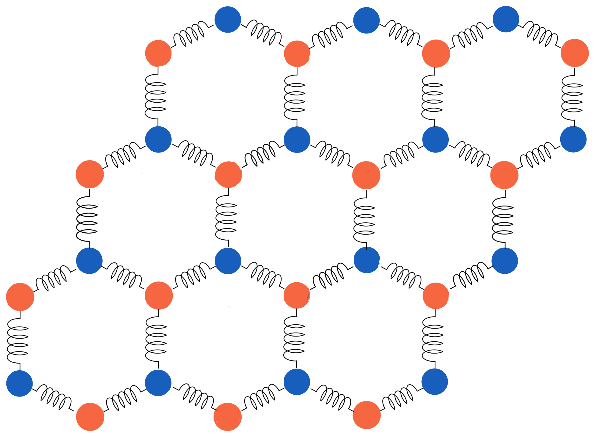
Figure 1: Schematic picture of the mechanical graphene. The system is composed of mass points and springs. The $A$ and $B$ sublattices are denoted by red and blue mass points, respectively.

II.1 Equation of motion without boundaries

Let us consider a system under the periodic boundary condition. The Fourier transformed displacement is written as

$$u_{\bm{k},\alpha}^{\mu}=\frac{1}{N}\sum_{\bm{R}}x_{\bm{R},\alpha}^{\mu}e^{i\bm{k}\cdot\bm{R}},$$ (1)

where $u_{\bm{k},\alpha}^{\mu}$ denotes the Fourier transformed displacement along $\mu$-direction $(\mu,\nu=x,y)$. $\alpha$ denotes sublattice $A,B$. The number of unit cells are denoted by $N$.

By applying the Fourier transformation, the equation of motion is written as,

$$\ddot{u}_{\bm{k},\alpha}^{\mu}=-D^{\mu\nu}_{\alpha\beta}(\bm{k})u^{\nu}_{\bm{k},\beta}-b\hat{1}\dot{u}^{\mu}_{\bm{k},\alpha},$$ (2)

with $\dot{u}^{\mu}_{\bm{k},\alpha}=\frac{du^{\mu}_{\bm{k},\alpha}}{dt}$. Summation over the repeated indices $\mu$, $\nu$ is assumed. The first and second terms describe the potential force and the frictional force proportional to the velocity respectively. The matrix $D(\bm{k})$ includes the mass $m$ of the mass points, the spring constant $\kappa$, and the tension $\eta$ as parameters. The explicit form of $D$ is given in Appendix A.

In a matrix form, the above equation is written as

$$\dot{\bm{\phi}}_{\bm{k}}(t) =M(\bm{k})\bm{\phi}_{\bm{k}}(t),$$ (3a)

$$M(\bm{k}) =\left(\begin{array}[]{cc}0&\hat{1}\\ -D(\bm{k})&-b\hat{1}\end{array}\right),$$ (3d)

with $\bm{\phi}_{\bm{k}}=(\bm{u}_{\bm{k}},\dot{\bm{u}}_{\bm{k}})^{T}$.

We note that the momentum region, where $M(\bm{k})$ cannot be diagonalized, appears as a ring. This ring is knowns as an SPER (for more details such as relevant symmetry of SPERs, see Appendix B). The above results imply that the SPER may affect the dynamics, which is explicitly demonstrated in Sec. IV.

II.2 dynamical properties for systems with boundaries

In the previous section, we have briefly reviewed the case under the periodic boundary condition. In this section, we describe how to obtain data in the wavenumber space from that in the real space when the system has the boundaries.

Let $x^{\mu}_{\bm{\tilde{R}}}$ be the displacement of a mass point at position $\bm{\tilde{R}}$. Then, the time-evolution of $x^{\mu}_{\bm{\tilde{R}}}$ is obtained from the equation of motion for $x^{\mu}_{\bm{\tilde{R}}}$ regardless of the presence/absence of the boundaries. For systems with the boundaries, the data in the wavenumber space is obtained by the Fourier integration. By applying the Fourier integration to $x^{\mu}_{\bm{\tilde{R}}}$, we can calculate the displacement $u^{\mu}_{\bm{k}}$ in the wavenumber space,

$$u^{\mu}_{\bm{k},\alpha}=\frac{1}{2\pi}\int_{-\infty}^{\infty}\int_{-\infty}^{\infty}d^{2}\bm{\tilde{R}}~{}x^{\mu}_{\bm{\tilde{R}},\alpha}e^{i\bm{k}\cdot\bm{\tilde{R}}},$$ (4)

Expressing $x^{\mu}_{\bm{\tilde{R}},\alpha}$ as a function of $\bm{\tilde{R}}$, we can write it as a sum of delta functions,

$$x_{\bm{\tilde{R}},\alpha}^{\mu}=\sum_{i}x_{\bm{\tilde{R}}_{i},\alpha}\delta(\bm{\tilde{R}}-\bm{R}_{i}).$$ (5)

Therefore, Eq. (4) can be expressed as,

$$u_{\bm{k},\alpha}^{\mu}=\sum_{i}x^{\mu}_{\bm{R}_{i},\alpha}e^{i\bm{k}\cdot\bm{R}_{i}},$$ (6)

where the sum is taken for all mass points belonging to sublattice $\alpha$.

Equation (6) is similar to Eq. (1). The difference between them is in the definition of wavenumber. In the latter case, the wavenumber is discrete, while in the former case, the wavenumber is continuous.

The difference between the free boundary and the fixed boundary is determined when solving the equation of motion for the displacement $x_{\bm{\tilde{R}}}$ in the real space.

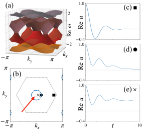
Figure 2: (a): The real-part of dispersion relation for the mechanical graphene. Band touching points correspond to the SPERs. (b): The SPERs for the mechanical graphene. Black dotted lines illustrate the Brillouin zone. (c)-(e): Time-evolution of $\mathrm{Re}u_{\bm{k}}$ at the specific point in the Brillouin zone. (c): Outside of the SPERs, the system shows a underdamping. (d): On the SPERs, the system shows a critical damping. (e): Inside of the SPERs, a overdamping is observed; $\mathrm{Re}u_{\bm{k}}$ remains positive. The data shown in this figure are for $(m,\kappa,\eta,b)=(1,1,0,1)$.

III dynamics of systems without boundary

In this section, we elucidate that the SPERs can be observed by examining the dynamics of displacements in the wavenumber space.

III.1 SPERs and types of damping

By numerically diagonalizing the matrix $M(\bm{k})$, we can obtain the dispersion relation $\omega(\bm{k})$ [see Fig. 2(a)]. In this figure, the band touching points form rings, which corresponds to the SPERs. The violation of the diagonalizability on the SPERs can also be observed in Fig. 2(b). This figure displays the momenta where $M(\bm{k})$ cannot be diagonalized.

In Sec. IV.2, we provides the numerical data elucidating that the SPERs govern the dynamics. Here, prior to the numerical simulation, we note the relation between $\omega(\bm{k})$ and the dispersion relation in the absence of the friction.

Applying a unitary transformation, the matrix $M(\bm{k})$ is rewritten as

$$\tilde{U}^{\dagger}(\bm{k})M(\bm{k})\tilde{U}(\bm{k})=\bigoplus_{n}\left(\begin{array}[]{cc}0&1\\ -\omega_{0n}^{2}&-b\end{array}\right),$$ (9)

where $\tilde{U}(\bm{k})$ is an unitary matrix (see Appendix C). Because the matrix appearing in the left-hand side of Eq. (9) is a set of $2\times 2$-matrix, we obtain

$$\omega_{n}(\bm{k})=-\frac{b}{2}i\pm\sqrt{\omega^{2}_{0n}(\bm{k})-\left(\frac{b}{2}\right)^{2}},$$ (10)

where $\omega^{2}_{0n}$ ($n=1,2,\ldots,\mathrm{dim}D$) denote eigenvalues of the matrix $D(\bm{k})$. Equation (10) indicates that the eigenvalues $\omega(\bm{k})$ take complex values inside of the SPERs. On the other hand, outside of the SPERs, $\omega(\bm{k})$ take real values. It means that the Fourier transformed displacement $u_{\bm{k}}^{\mu}$ behaves differently inside and outside of the SPERs. Specifically, the underdamping (overdamping) is observed outside (inside) of the SPERs. Additionally, on the SPERs, $u_{\bm{k}}$ become the critical damping, which converges most quickly. In Sec. IV.2, we discuss the above behaviors in details.

III.2 Numerical demonstration of dynamics

We demonstrate that the SPERs separates regions of overdamping and regions of underdamping. This fact indicates that the SPERs govern the dynamics.

In the following, we set $u_{\bm{k}}(t=0)$ to $u_{\bm{k}}(t=0)=1$ as the initial condition. This condition corresponds to the case where the mass point at the origin is displaced at $t=0$.

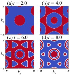
Figure 3: Snapshots of time-evolution of $\mathrm{Re}u_{\bm{k}}$ over all wavenumber (initial condition is $u_{\bm{k}}$ = 1 for all $\bm{k}$). In red (blue) regions, sign of $\mathrm{Re}u_{\bm{k}}$ is plus (minus). White region means $|\mathrm{Re}u_{\bm{k}}|<0.005$. Inside the SPERs, the sign remains positive. In the region around the $\Gamma$ point [i.e., $\bm{k}=(0,0)$], the sign of displacement is unchanged up to $t=6.0$. The boundary of this region corresponds to the SPER.

III.2.1 Specific wavenumber

Let us first discuss the time-evolution for given momenta. Figures 2(c)-2(e) indicate the dynamics of displacement for given wave numbers denoted by a cross, a cycle, and a square in Fig. 2(b).

The contribution of the time-evolution of $u_{\bm{k}}$ can be expressed as $e^{i\omega(\bm{k})t}=e^{-\mathrm{Im}\omega(\bm{k})\cdot t}\cdot e^{i\mathrm{Re}\omega(\bm{k})\cdot t}$. Thus, in addition to the oscillation, damping occurs as $\omega$ takes a complex value [see Fig. 2(c)]. As we approach closer to the inner side of the SPER [i.e., the region denoted by the arrow in Fig. 2(b)], the oscillations reach a critical damping on the SPER, where $\omega$ becomes purely imaginary [see Fig. 2(d)]. Inside of the SPER, overdamping is observed [see Fig. 2(e)]. Here, we note that oscillation is observed even inside of the SPERs and on the SPERs. This is because the gray and orange bands in Fig. 2(a) are also involved in the dynamics.

The displacement insides of the SPERs decays slower than that on the SPERs. This behavior can be understood as follows. Inside of the SPERs, we have two eigenvalues $\omega_{n}=-ib/2\pm i\sqrt{|\omega^{2}_{0n}(\bm{k})-\frac{b}{2}|}$. In contrast, on the SPERs, we have $\omega=-ib/2$ due to band touching. Because the eigenmodes with $\omega_{n}=-ib/2+i\sqrt{|\omega^{2}_{0n}(\bm{k})-\frac{b}{2}|}$ decays slower than the modes with $\omega_{n}=-ib/2$, the displacement inside of the SPERs decays slower than that on the SPERs.

III.2.2 Over all wavenumber

The time-evolution of the displacement in the wavenumber space is shown in Fig. 3. This figure indicates that $u_{\bm{k}}$ changes its sign. The red (blue) region means $u_{\bm{k}}$ takes positive (negative) values. The white region means $u_{\bm{k}}=0$. We confirm that inside of the SPERs $u_{\bm{k}}$ remains positive even if time passes. while outside of the SPERs, the sign of $u_{\bm{k}}$ changes as time passes.

This result indicates that the SPERs for the mechanical graphene can be observed by examining the time-evolution in the wavenumber space.

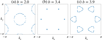
Figure 4: (a), (b) and (c): The SPERs for $b=2.0$, $3.4$ and $3.9$, respectively. The data shown in this figure are obtained for momentum points $\bm{k}_{0}$ satisfying $|\mathrm{det}M(\bm{k}_{0})|<0.005.$

IV Lifshitz transition for mechanical systems

In this section, we point out that the mechanical graphene with the friction exhibits a behavior which is analogous to the Lifshitz transition in quantum systems. The Lifshitz transition is known as changes of the connectivity of the Fermi surface for electronic systems at zero temperature; shifting the Fermi energy changes the connectivity of the Fermi surface. Here, for given Fermi energy, the Fermi surface appears as a cross section of the bands and the Fermi energy.

IV.1 Periodic boundary condition

Firstly, we point out that the SPERs in the mechanical system are similar to the Fermi surface of an electron system. This correspondence can be seen in Eq. (10). This equation indicates that the SPERs emerge as cross section of the dispersion relation $\omega_{0n}(\bm{k})$ and half of the frication coefficient $b/2$. Specifically, at momenta satisfying,

$$\omega_{0n}(\bm{k})=\frac{b}{2},$$ (11)

$M(\bm{k})$ becomes exceptional.

Therefore, with increasing the frictional coefficient, the connectivity of the SPERs changes. Figure 4 plots the SPERs for several values of the frictional coefficient $b$. This figure indicates that with increasing $b$ from $b=2.0$, the SPERs shrinks to points [see Fig. 4(a) and 4(b)]. Further increasing $b$, the SPERs emerges again [see Fig. 4(c)]. This change of the connectivity is analogous to the Lifshitz transition of electron systems.

The above “Lifshitz transition” in the mechanical system also affects the dynamical properties. Figure 5 shows that dynamics of $u_{\bm{k}}$ for $b=3.0$ under the periodic boundary condition. This figure shows that $u_{\bm{k}}$ behaves the overdamping (underdamping) outside (inside) of the SPERs. This behavior for $b=3.0$ is in sharp contrast to that for $b=1.0$. For $b=3.0$, the underdamping is observed inside of the SPERs [i.e., the region denoted by the arrow in Fig. 5(a)] while the overdamping is observed outside of the SPERs. Namely, compared to the case for $b=1.0$, the region of overdamping and that of the underdamping are exchanged.

In the above, we have seen that connectivity of the SPERs changes depending on the frictional force, which is analogous to the Lifshitz transition of electron systems. Our numerical simulation has elucidated that the change of the connectivity also affects the dynamical properties.

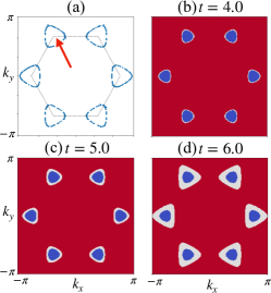
Figure 5: Dynamics of the Fourier transformed displacement $u_{\bm{k}}$ for $b=3.0$ with the periodic boundary. (a): The SPERs for $b=3.0$. (b), (c), and (d): Snapshots of time-evolution of $u_{\bm{k}}$ over all wavenumber (initial condition is $u_{\bm{k}}$ = 1 for all $\bm{k}$) at $t=4.0$, $5.0$, and $6.0$, respectively. In the region around the $K$ point [i.e., $\bm{k}=(2\pi/3\sqrt{3},2\pi/3)$], the sign of the displacement is unchanged up to $t=6.0$. The boundary of this region corresponds to the SPER.

IV.2 Fixed boundary condition

So far, we have analyzed the system under the periodic boundary condition. In this section, we investigate the “Lifshitz transition” for systems with the boundaries because most of experiments are carried out for systems with boundaries.

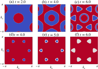
Figure 6: (a), (b), and (c): [(d), (e), and (f):] Snapshot of the dynamics of $u_{\bm{k}}$ at $t=2.0$, $4.0$, and $6.0$ [$t=4.0$, $5.0$, and $6.0$] with the fixed boundary condition at $b=1.0$ [$b=3.0$] respectively. One can see that changing the value of $b$ causes the dynamics to switch between the inside and outside of the SPERs (initial condition is $u_{\bm{k}}$ = 1 for all $\bm{k}$). In panels (a)-(c), the sign of displacement is unchanged up to $t=6.0$ for the region around the $\Gamma$ point [i.e., $\bm{k}=(0,0)$]. The boundary of this region corresponds to the SPER. In panels (d)-(f), the sign of the displacement is unchanged up to $t=6.0$ for the region around the $K$ point [i.e., $\bm{k}=(2\pi/3\sqrt{3},2\pi/3)$]. The boundary of this region corresponds to the SPER.

Figure 6 shows the results of the numerical simulation of the mechanical graphene with the fixed boundary condition. Specifically, the numerical data are obtained for the system composed of 242 sites (for more details see Fig. 9 of Appendix D). For $b=1.0$, the sign of $u_{\bm{k}}$ does not change during the time-evolution in the region surrounded by the SPERs [see Figs. 6(a)-6(c)]. In other words, the overdamping occur in this region. For $b=3.0$, it can be seen that the region of the overdamping expands. The above results are consistent with the results without the boundaries, which indicates the “Lifshitz transition” is also observed for the system under the fixed boundary conditions by examining the dynamics of the displacement in the wavenumber space.

The results with and without the boundaries are consistent when the oscillations do not reach to the boundaries of the system. When the oscillations propagate to the boundaries, the displacement in the wavenumber space behaves differently from the results for the periodic boundary condition due to the influence of reflected waves. Therefore, in order to observe the SPERs, the size of the system must be large enough so that the effect of the boundaries can be neglected (see Appendix D.2). Although Fig. 6 shows the results for the fixed boundary condition, the same results can be obtained for the free boundary condition, since the results are not affected by the reflected wave unless the oscillation reaches to the boundaries.

V Summary

Despite the previous theoretical prediction of the SPERs in mechanical systems, the experimental observation has not been accomplished yet. In this paper, prior to experimental realization, we have theoretically addressed the following issues: (i) how the emergence of the SPERs affects dynamical behaviors which are experimentally accessible; (ii) what is the proper formulation of the Fourier transform in the systems with the boundaries.

Our results elucidate that the SPERs for the mechanical graphene govern the dynamics in the wavenumber space. Outside of the SPERs, the Fourier transformed displacement $u_{\bm{k}}$ shows the underdamping, while inside of the SPERs, $u_{\bm{k}}$ shows the overdamping (i.e., the sign of $u_{\bm{k}}$ remains plus). On the SPERs, critical damping is observed, which switches from the overdamping to the underdamping.

Furthermore, we have observed the phenomenon corresponding the Lifshitz transition of electron systems. Increasing the friction coefficient, connectivity of the SPERs changes. This change of the connectivity, analogous to the Lifshitz transition, is observed by examining the dynamical properties.

VI Acknowledgements

This work is partly supported by JSPS KAKENHI Grants No. 17H06138, No. JP20H04627, and No. JP21K13850.

Appendix A Details of the mechanical graphene

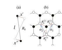
Figure 7: (a): Definitions of $\bm{R}_{0}$, $\bm{x^{\prime}}$, and $\bm{x^{\prime\prime}}$. (b): Definitions of unit vectors $\bm{a}_{1}$ and $\bm{a}_{2}$, the vectors connecting the nearest neighbor mass points $\bm{R}_{0}$.

The model treated in this paper is the mechanical graphene, which is composed of mass points and springs (see Fig. 1). Mass points are aligned in honeycomb lattice. Here, we obtain the motion of equation of the mechanical graphene.

A.1 In case of no friction

First, to find the Lagrangian of the system, we focus the unit cell which is plotted in Fig. 7. Then, the elastic energy is written as

$$U_{s}=\frac{1}{2}\kappa(l-l_{0}),$$ (12)

where $l$ is the length of the spring at the moment, and $l_{0}$ is the natural length of the spring. If $U_{s}$ is expanded to the second order in $\delta\bm{x}=\bm{x}^{\prime}-\bm{x}^{\prime\prime}$, we get

$$U_{s} =\frac{1}{2}\kappa\left((R_{0}-l_{0})^{2}+\right.$$

$$\quad\left.2(R_{0}-l_{0})\hat{\bm{R}}_{0}\cdot\delta\bm{x}+\delta x_{\mu}\gamma_{\hat{\bm{R}}_{0}}^{\mu\nu}\delta x_{\nu}\right),$$ (13)

$$\gamma^{\mu\nu}_{\hat{\bm{R}}_{0}} =(1-\eta)\delta^{\mu\nu}+\eta\hat{R}_{0}^{\mu}\hat{R}_{0}^{\nu},$$ (14)

with $\bm{\hat{R}}_{0}=\bm{R}_{0}/|\bm{R}_{0}|$. Summation over the repeated indices $\mu$, $\nu$ is assumed.

Then, the Lagrangian of this system becomes

$$L =T-V,$$ (15)

$$T =\frac{1}{2}\sum_{\bm{R}a}\dot{x}^{\mu}_{\bm{R}a}\dot{x}^{\mu}_{\bm{R}a},$$ (16)

$$V =\frac{1}{2}\kappa\sum_{\langle\bm{R}^{\prime}a\bm{R}b\rangle}(x^{\mu}_{\bm{\bar{R^{\prime}}}a}-x^{\mu}_{\bm{\bar{R}}b})\gamma^{\mu\nu}_{\bm{\bar{R^{\prime}}}a-\bm{\bar{R}}b}(x^{\nu}_{\bm{\bar{R^{\prime}}}a}-x^{\nu}_{\bm{\bar{R}}b}),$$ (17)

where $\bm{\bar{R}_{a}}$ is a position of the sublattice associated with the lattice point at $\bm{R}$. Summation over $\langle\bm{R}^{\prime}a\bm{R}b\rangle$ means to take sum with respect to adjacent qualities. Assuming the periodic boundary condition, after the Fourier transformation,

$$x_{\bm{R}a}=\frac{1}{N}\sum_{\bm{k}}e^{i\bm{k}\cdot\bm{R}}u_{\bm{k}a}^{\mu},$$ (18)

the Lagrangian is rewritten as

$$L =\frac{1}{N}\sum_{\bm{k}}L_{\bm{k}},$$ (19)

$$L_{\bm{k}} =\frac{1}{2}\sum_{a}\dot{u}^{\mu}_{\bm{k}a}\dot{u}^{\mu}_{-\bm{k}a}-\frac{1}{2}\sum_{ab}D^{\mu\nu}_{ab}u_{\bm{k}a}u_{-\bm{k}b},$$ (20)

where $D^{\mu\nu}_{ab}=D(\bm{k})$,

$$D(\bm{k}) =3\kappa\left(1-\frac{\eta}{2}\right)\hat{1}+\left(\begin{array}[]{cc}0&D_{AB}(\bm{k})\\ D_{AB}^{\dagger}(\bm{k})&0\end{array}\right),$$ (21c)

$$D_{AB}(\bm{k}) =\kappa(\gamma_{1}e^{-i\bm{k}\cdot\bm{a}_{1}}+\gamma_{2}e^{-i\bm{k}\cdot\bm{a}_{2}}+\gamma_{3}),$$ (21d)

$$\gamma_{1} =(1-\eta)\left(\begin{array}[]{cc}1&0\\ 0&1\end{array}\right)+\eta\left(\begin{array}[]{cc}\frac{3}{4}&\frac{\sqrt{3}}{4}\\ \frac{\sqrt{3}}{4}&\frac{3}{4}\end{array}\right),$$ (21i)

$$\gamma_{2} =(1-\eta)\left(\begin{array}[]{cc}1&0\\ 0&1\end{array}\right)+\eta\left(\begin{array}[]{cc}\frac{3}{4}&-\frac{\sqrt{3}}{4}\\ -\frac{\sqrt{3}}{4}&\frac{3}{4}\end{array}\right),$$ (21n)

$$\gamma_{3} =(1-\eta)\left(\begin{array}[]{cc}1&0\\ 0&1\end{array}\right)+\eta\left(\begin{array}[]{cc}0&0\\ 0&1\end{array}\right),$$ (21s)

Then, the equation of motion is given by

$$\ddot{u}_{\bm{k}}^{\mu}=-D^{\mu\nu}_{\alpha\beta}(\bm{k})u^{\nu}_{\bm{k}}.$$ (22)

A.2 In case of friction

Next, we consider the case of the friction. Then, the equation of motion is rewritten as

$$\ddot{u}_{\bm{k}}^{\mu}=-D^{\mu\nu}_{\alpha\beta}(\bm{k})u^{\nu}_{\bm{k}}+\Gamma_{0\alpha\beta}^{\mu\nu}(\bm{k})\dot{u}^{\nu}_{\bm{k}},$$ (23)

The first and second terms describe the potential force and the frictional force proportional to the velocity respectively.

In the matrix form, the above equation is rewritten as

$$\dot{\bm{\phi}}_{\bm{k}}(t) =M(\bm{k})\bm{\phi}_{\bm{k}}(t),$$ (24a)

$$M(\bm{k}) =\left(\begin{array}[]{cc}0&\hat{1}\\ -D(\bm{k})&\Gamma_{0}(\bm{k})\end{array}\right),$$ (24d)

with $\bm{\phi}_{\bm{k}}=(\bm{u}_{\bm{k}},\dot{\bm{u}}_{\bm{k}})^{T}$.

When the friction is homogeneous, matrix $\Gamma_{0}(\bm{k})$ is represented by $\Gamma_{0}(\bm{k})=-b\hat{1}$.

In this way, the mechanical graphene with the friction can be represented by the eigenvalue equation of non-Hermitian matrix. Practically, we can get eigenvalues by diagonalizing $M(\bm{k})$.

A.3 Numerical demonstration

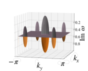
Figure 8: The imaginary-part of dispersion relation for the mechanical graphene.

We demonstrate that the mechanical graphene hosts the SPERs. By diagonalizing the Matrix $M(\bm{k})$, we can obtain the dispersion relations $\omega(\bm{k})$ for $\eta=0$ and $b=1$ which is plotted in Fig. 2(a) and Fig. 8. We can see that rings of band touching points, which is caused by the friction. At the rings of band-touching points, the Hamiltonian becomes defective. In other words, the SPERs emerge for the mechanical graphene. The emergence of SPERs can also be seen in Fig. 2(b). This figure shows that wavenumber points in the Brillouin zone where the Hamiltonian is defective. In other words, these points mean that the determinant of the matrix $U(\bm{k})$ becomes zero. Here, $U(\bm{k})$ is the matrix that lists all eigenvectors of $M(\bm{k})$. The SPERs are characterized by the topological quantity called 0th Chern number.

Appendix B Relation between symmetry and EPs

When there is symmetry in the system, the EPs change the form. In this section, we discuss the symmetry of the mechanical system. Additionally, we also show that EPs become the rings by symmetry.

B.1 Hamiltonian of the mechanical graphene

In order to discuss the symmetry, we describe the corresponding Hamiltonian in the mechanical graphene.

Because the matrix $D(\bm{k})$ is Hermitian and positive semidefinite, using the Hermitian matrix $Q(\bm{k})$, it can be written as follows

$$D(\bm{k})=Q^{2}(\bm{k}).$$ (25)

Therefore, Eq. (24a) can be rewritten as

$$i\frac{\partial}{\partial t}\psi(t) =H(\bm{k})\psi(t),$$ (26a)

$$H(\bm{k}) =\left(\begin{array}[]{cc}0&Q(\bm{k})\\ Q(\bm{k})&i\Gamma_{0}(\bm{k})\end{array}\right),$$ (26d)

with

$$\psi(t) =\left(\begin{array}[]{cc}Q(\bm{k})&0\\ 0&i\hat{1}\end{array}\right)\phi(t).$$ (26g)

The matrix $H(\bm{k})$ and $M(\bm{k})$ in Eq. (24a) have the same eigenvalues. Therefore, the dynamics of the system can be described by the matrix $H(\bm{k})$. In addition, since Eq. (26a) is essentially the same as the Schrödinger equation, the matrix $H(\bm{k})$ can be regarded as Hamiltonian of the system. In the following, we use Hamiltonian $H(\bm{k})$ to discuss symmetry.

When $i\Gamma(\bm{k})$ is Hermitian (e.g. $\Gamma_{0}(\bm{k})=-b\hat{1}$), the system has extended chiral symmetry,

$$\tau_{3}H^{\dagger}(\bm{k})\tau_{3}=-H(\bm{k}),$$ (27)

regardless of its detailed form ($\tau$’s are Pauli matrices).

B.2 Symmetry and exceptional points

Here we show that in a two-dimensional system, EPs form rings when there is a symmetry such as Eq. (27).

For simplicity, we consider the case where the system can be described by $2\times 2$ Hamiltonian $H(\bm{k})$. In general, $2\times 2$ matrix can be written using Pauli matrices $\tau$’s as

$$H(\bm{k})=\sum_{\mu=0,1,2,3}\left[b_{\mu}(\bm{k})+id_{\mu}(\bm{k})\right]\tau_{\mu},$$ (28)

with $b_{\mu},d_{\mu}\in\mathbb{R}~{}(\mu=0,1,2,3)$. The eigenvalues of $H(\bm{k})$ are as follows

$$E_{\pm}=b_{0}+id_{0}\pm\sqrt{b^{2}-d^{2}+2i\bm{b}\cdots\bm{d}},$$ (29)

with $\bm{b}=(b_{1},b_{2},b_{3})^{T}$ and $\bm{d}=(d_{1},d_{2},d_{3})^{T}$. As can be seen from Eq. (29), the band of the system touches the point where the content of the root number becomes zero. That is, the band touches at the points which the following two equations hold

$$b^{2}-d^{2}=0,$$ (30a)

$$\bm{b}\cdot\bm{d}=0.$$ (30b)

Since the system has two dimensions and there are two conditionals, $\bm{k}$ satisfying the conditionals appears as zero-dimensional objects (points). At this points, if we do not apply fine tune, the Hamiltonian $H(\bm{k})$ is no longer diagonalizable. That is, these points are EPs.

Next, we consider the case where the system has symmetry as Eq (27). In this case, the Hamiltonian can be expressed as

$$H(\bm{k})=id_{0}\tau_{0}+b_{1}\tau_{1}+b_{2}\tau_{2}+id_{3}\tau_{3}.$$ (31)

That is, $\bm{b}$ and $\bm{d}$ are respectively as follows

$$\bm{b} =(b_{1},b_{2},0)^{T},$$ (32a)

$$\bm{d} =(0,0,d_{3})^{T}.$$ (32b)

Therefore, one of the conditionals (30b) is automatically satisfied by symmetry. Since the system has two dimensions and there are one conditionals, $\bm{k}$ satisfying the conditionals appears as one-dimensional objects (rings). That is, these points are the SPERs.

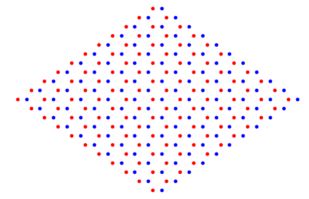
Figure 9: Sketch of the mechanical graphene used in the numerical calculations. There are 242 mass points in total. The unit cells are arranged so that it forms a rhombus. We consider the fixed boundary condition where the mass points of the boundaries are connected to the wall by springs.

Appendix C Properties of SPERs

In fact, we can obtain the eigenvalue of $M(\bm{k})$ analytically. When we consider the condition with the homogeneous friction (in other words, matrix $\Gamma_{0}$ can be represented by $-b\hat{1}$), we can block diagonalize $M(\bm{k})$ using matrix $U(\bm{k})$ which diagonalize $D(\bm{k})$,

$$\left(\begin{array}[]{cc}U(\bm{k})&0\\ 0&U(\bm{k})\end{array}\right)\left(\begin{array}[]{cc}0&\hat{1}\\ -D(\bm{k})&-b\hat{1}\end{array}\right)\left(\begin{array}[]{cc}U^{\dagger}(\bm{k})&0\\ 0&U^{\dagger}(\bm{k})\end{array}\right)$$ (39)

$$=\left(\begin{array}[]{cc}0&\hat{1}\\ -\hat{\omega}^{2}_{0}(\bm{k})&-b\hat{1}\end{array}\right),$$ (42)

where $\hat{\omega}_{0}$ denotes the diagonal matrix with eigenvalues of $D(\bm{k})$ on diagonal components. The above equation can be rewritten as

$$\left(\begin{array}[]{cc}0&\hat{1}\\ -\hat{\omega}^{2}_{0}(\bm{k})&-b\hat{1}\end{array}\right)=\bigoplus_{n}\left(\begin{array}[]{cc}0&1\\ -\omega_{0n}^{2}&-b\end{array}\right),$$ (47)

where $n$ denotes the number of bands for $D(\bm{k})$. From this equation, we can obtain the eigenvalues of $M(\bm{k})$,

$$\omega(\bm{k})=-\frac{b}{2}i\pm\sqrt{\omega_{0n}^{2}(\bm{k})-\left(\frac{b}{2}\right)^{2}}.$$ (48)

This relation indicates that the SPERs emerge to satisfy the following equation,

$$\omega_{0n}(\bm{k})=\frac{b}{2}.$$ (49)

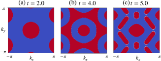
Figure 10: The dynamics of $u_{\bm{k}}$ when the number of mass points is 50 with the fixed boundary (initial condition is $u_{\bm{k}}$ = 1 for all $\bm{k}$). (a), (b), and (c): Snapshots of time-evolution of $u_{\bm{k}}$ over all wavenumber (initial condition is $u_{\bm{k}}$ = 1 for all $\bm{k}$) at $t=2.0$, $4.0$, and $5.0$, respectively.

Appendix D System used in the numerical calculation

In this section, we show the details of the system that we actually considered when performing the numerical calculations. We also discuss how the dynamics is affected by the boundary when the system is small.

D.1 Cases not affected by boundaries

Figure 9 shows a sketch of the mechanical graphene used in the numerical calculations. This system has boundaries, i.e., the mass points at the boundaries are connected to the wall by the spring. The same results as for the periodic boundary condition are obtained even when the system has the boundaries until the oscillation is transmitted to the mass points at the boundaries.

D.2 Cases affected by boundaries

We show that in a system with a boundary, the results for an infinite system cannot be reproduced if the system is affected by reflected waves.

Figure 10 shows the time-evolution of $u_{\bm{k}}$ when the number of mass points is 50. Up to a certain time, the results are consistent for an infinite system, but after the time, the results are clearly not consistent. This is because the vibrations reach the edges and are affected by the reflected waves.

References

- Kane and Mele (2005) C. L. Kane and E. J. Mele, Physical Review Letters 95 (2005), 10.1103/physrevlett.95.146802.
- Bernevig et al. (2006) B. A. Bernevig, T. L. Hughes, and S.-C. Zhang, Science 314, 1757–1761 (2006).
- Konig et al. (2007) M. Konig, S. Wiedmann, C. Brune, A. Roth, H. Buhmann, L. W. Molenkamp, X.-L. Qi, and S.-C. Zhang, Science 318, 766–770 (2007).
- Hatsugai (1993a) Y. Hatsugai, Phys. Rev. B 48, 11851 (1993a).
- Hatsugai (1993b) Y. Hatsugai, Phys. Rev. Lett. 71, 3697 (1993b).
- Hasan and Kane (2010) M. Z. Hasan and C. L. Kane, Reviews of Modern Physics 82, 3045–3067 (2010).
- Qi and Zhang (2011) X.-L. Qi and S.-C. Zhang, Reviews of Modern Physics 83, 1057–1110 (2011).
- Haldane and Raghu (2008) F. D. M. Haldane and S. Raghu, Physical Review Letters 100 (2008), 10.1103/physrevlett.100.013904.
- Wang et al. (2009) Z. Wang, Y. Chong, J. D. Joannopoulos, and M. Soljačić, Nature 461, 772 (2009).
- Raghu and Haldane (2008) S. Raghu and F. D. M. Haldane, Phys. Rev. A 78, 033834 (2008).
- Ningyuan et al. (2015) J. Ningyuan, C. Owens, A. Sommer, D. Schuster, and J. Simon, Phys. Rev. X 5, 021031 (2015).
- Albert et al. (2015) V. V. Albert, L. I. Glazman, and L. Jiang, Phys. Rev. Lett. 114, 173902 (2015).
- Lee et al. (2018) C. H. Lee, S. Imhof, C. Berger, F. Bayer, J. Brehm, L. W. Molenkamp, T. Kiessling, and R. Thomale, Communications Physics 1 (2018), 10.1038/s42005-018-0035-2.
- Yoshida et al. (2020) T. Yoshida, T. Mizoguchi, and Y. Hatsugai, Phys. Rev. Research 2, 022062 (2020).
- Süsstrunk and Huber (2016) R. Süsstrunk and S. D. Huber, Proceedings of the National Academy of Sciences 113, E4767–E4775 (2016).
- Kariyado and Hatsugai (2015) T. Kariyado and Y. Hatsugai, Scientific Reports 5 (2015), 10.1038/srep18107.
- Kane and Lubensky (2013) C. L. Kane and T. C. Lubensky, Nature Physics 10, 39–45 (2013).
- Takahashi et al. (2017) Y. Takahashi, T. Kariyado, and Y. Hatsugai, New Journal of Physics 19, 035003 (2017).
- Takahashi et al. (2019) Y. Takahashi, T. Kariyado, and Y. Hatsugai, Physical Review B 99 (2019), 10.1103/physrevb.99.024102.
- Wakao et al. (2020) H. Wakao, T. Yoshida, H. Araki, T. Mizoguchi, and Y. Hatsugai, Physical Review B 101 (2020), 10.1103/physrevb.101.094107.
- Prodan and Prodan (2009) E. Prodan and C. Prodan, Physical Review Letters 103 (2009), 10.1103/physrevlett.103.248101.
- Po et al. (2016) H. C. Po, Y. Bahri, and A. Vishwanath, Physical Review B 93 (2016), 10.1103/physrevb.93.205158.
- Paulose et al. (2015) J. Paulose, B. G.-g. Chen, and V. Vitelli, Nature Physics 11, 153 (2015).
- Rocklin et al. (2016) D. Z. Rocklin, B. G. Chen, M. Falk, V. Vitelli, and T. Lubensky, Physical Review Letters 116 (2016), 10.1103/physrevlett.116.135503.
- Wang et al. (2015) P. Wang, L. Lu, and K. Bertoldi, Physical Review Letters 115 (2015), 10.1103/physrevlett.115.104302.
- Socolar et al. (2017) J. E. S. Socolar, T. C. Lubensky, and C. L. Kane, New Journal of Physics 19, 025003 (2017).
- Bergholtz et al. (2021) E. J. Bergholtz, J. C. Budich, and F. K. Kunst, Reviews of Modern Physics 93 (2021), 10.1103/revmodphys.93.015005.
- Shen et al. (2018) H. Shen, B. Zhen, and L. Fu, Physical Review Letters 120 (2018), 10.1103/physrevlett.120.146402.
- Shen and Fu (2018) H. Shen and L. Fu, Physical Review Letters 121 (2018), 10.1103/physrevlett.121.026403.
- Ghatak and Das (2019) A. Ghatak and T. Das, Journal of Physics: Condensed Matter 31, 263001 (2019).
- Xiong et al. (2016) Y. Xiong, T. Wang, X. Wang, and P. Tong, “Comment on ”anomalous edge state in a non-hermitian lattice”,” (2016), arXiv:1610.06275 [quant-ph] .
- Kozii and Fu (2017) V. Kozii and L. Fu, “Non-hermitian topological theory of finite-lifetime quasiparticles: Prediction of bulk fermi arc due to exceptional point,” (2017), arXiv:1708.05841 [cond-mat.mes-hall] .
- Hatano and Nelson (1996) N. Hatano and D. R. Nelson, Physical Review Letters 77, 570–573 (1996).
- Bender and Boettcher (1998) C. M. Bender and S. Boettcher, Physical Review Letters 80, 5243–5246 (1998).
- Fukui and Kawakami (1998) T. Fukui and N. Kawakami, Phys. Rev. B 58, 16051 (1998).
- Sone et al. (2020) K. Sone, Y. Ashida, and T. Sagawa, Nature Communications 11 (2020), 10.1038/s41467-020-19488-0.
- Lee (2016) T. E. Lee, Physical Review Letters 116 (2016), 10.1103/physrevlett.116.133903.
- Gong et al. (2017) Z. Gong, S. Higashikawa, and M. Ueda, Physical Review Letters 118 (2017), 10.1103/physrevlett.118.200401.
- Guo et al. (2009) A. Guo, G. J. Salamo, D. Duchesne, R. Morandotti, M. Volatier-Ravat, V. Aimez, G. A. Siviloglou, and D. N. Christodoulides, Phys. Rev. Lett. 103, 093902 (2009).
- Rüter et al. (2010) C. E. Rüter, K. G. Makris, R. El-Ganainy, D. N. Christodoulides, M. Segev, and D. Kip, Nature Physics 6, 192 (2010).
- Regensburger et al. (2012) A. Regensburger, C. Bersch, M. A. Miri, G. Onishchukov, D. N. Christodoulides, and U. Peschel, Nature 488, 167 (2012).
- Zhen et al. (2015) B. Zhen, C. W. Hsu, Y. Igarashi, L. Lu, I. Kaminer, A. Pick, S.-L. Chua, J. D. Joannopoulos, and M. Soljačić, Nature 525, 354–358 (2015).
- Hassan et al. (2017) A. U. Hassan, B. Zhen, M. Soljačić, M. Khajavikhan, and D. N. Christodoulides, Physical Review Letters 118 (2017), 10.1103/physrevlett.118.093002.
- Zhou et al. (2018) H. Zhou, C. Peng, Y. Yoon, C. W. Hsu, K. A. Nelson, L. Fu, J. D. Joannopoulos, M. Soljačić, and B. Zhen, Science 359, 1009–1012 (2018).
- Carlström and Bergholtz (2018) J. Carlström and E. J. Bergholtz, Physical Review A 98 (2018), 10.1103/physreva.98.042114.
- Yoshida et al. (2018) T. Yoshida, R. Peters, and N. Kawakami, Physical Review B 98 (2018), 10.1103/physrevb.98.035141.
- Yoshida et al. (2019) T. Yoshida, R. Peters, N. Kawakami, and Y. Hatsugai, Physical Review B 99 (2019), 10.1103/physrevb.99.121101.
- Budich et al. (2019) J. C. Budich, J. Carlström, F. K. Kunst, and E. J. Bergholtz, Physical Review B 99 (2019), 10.1103/physrevb.99.041406.
- Okugawa and Yokoyama (2019) R. Okugawa and T. Yokoyama, Physical Review B 99 (2019), 10.1103/physrevb.99.041202.
- Zhou and Lee (2019) H. Zhou and J. Y. Lee, Physical Review B 99 (2019), 10.1103/physrevb.99.235112.
- Xu et al. (2017) Y. Xu, S.-T. Wang, and L.-M. Duan, Physical Review Letters 118 (2017), 10.1103/physrevlett.118.045701.
- Yoshida and Hatsugai (2019) T. Yoshida and Y. Hatsugai, Physical Review B 100 (2019), 10.1103/physrevb.100.054109.