figurem tablem

Direct validation of dune instability theory
— Supplementary Information —

Ping Lü^1,∗, Clément Narteau^2,∗, Zhibao Dong¹,

Philippe Claudin³, Sébastien Rodriguez², Zhishan An⁴,

Laura Fernandez-Cascales², Cyril Gadal², Sylvain Courrech du Pont⁵

• School of Geography and Tourism, Shaanxi Normal University, 620 Chang’an West Avenue, Xi’an, Shaanxi 710119, China.

• Université de Paris, Institut de physique du globe de Paris, CNRS, F-75005 Paris, France.

• Physique et Mécanique des Milieux Hétérogènes, UMR 7636 CNRS, ESPCI PSL Research Univ, Sorbonne Univ, Université de Paris, 10 rue Vauquelin, 75005 Paris, France.

• Northwest Institute of Eco-Environment and Resources Donggang West Road 320, Lanzhou, Gansu Province 730000, China.

• Laboratoire Matière et Système Complexes, Université de Paris. UMR 7057 CNRS, Bâtiment Condorcet, 10 rue Alice Domon et Léonie Duquet, 75205 Paris Cedex 13, France.

  ^∗To whom correspondence should be addressed. E-mail: lvping@snnu.edu.cn, narteau@ipgp.fr

1 Supplementary Note 1
Wind data

We installed a 2 m high wind tower in the center of our new experimental site and collected the wind data of the local airport located 10 km east. We use the local tower for the measurements of the transport threshold and the saturation length (see Figs. 2 and 3 of the main manuscript). We check the consistency between the local wind data and those collected at the airport. For the long-term experiment, we only use the wind data of the local airport.

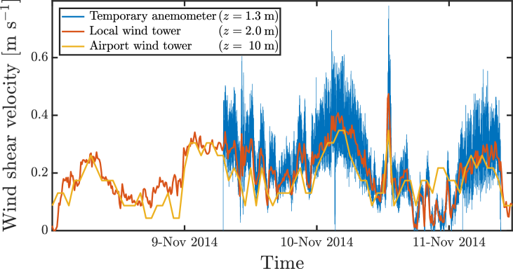
Figure S1: Comparison of wind speed data. Wind shear velocity derived from temporary wind speed measurements made during the threshold experiment (blue) and simultaneous measurements obtained on the local (red) and the airport wind towers (yellow). There is a general agreement between all these data sets.

Fig. S1 shows the shear velocity derived from a local wind measurement, the 2 m high wind tower and the airport meteorological tower during the transport threshold experiment (see Fig. 2 of the main manuscript). All these data are consistent with each other. As a consequence, the threshold shear stress derived from the local measurement can be extrapolated to other wind data to compute sand fluxes (Sec. 3).

2 Supplementary Note 2
Grain size distribution

The landscape-scale experiment site is located close to the oasis city of Shapotu at 8 km from the Yellow River in the Tengger Desert, which covers an area of about 36,700 km² in the northwest part of the Zhongwei County in the Ningxia Hui Autonomous Region of the People’s Republic of China (37° 31´ N, 105° E). This desert is characterized by a lognormal grain size distribution with a mean value $d$=190$\leavevmode\nobreak\ \mu$m (Fig. S2).

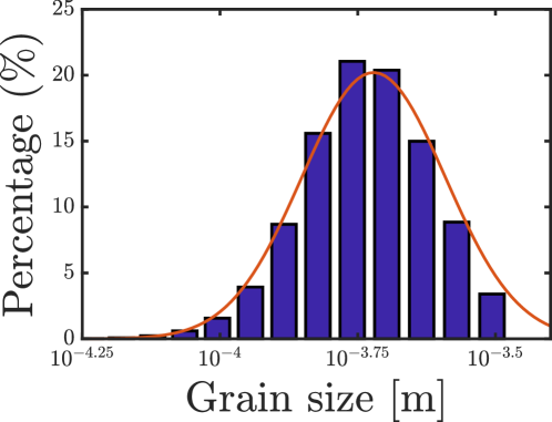
Figure S2: Grain size distribution in the Tengger Desert. The line is the best fit using a lognormal distribution with a mean value $d=190\;\mu{\rm m}\approx 10^{-3.72}\;{\rm m}$.

Variable	Units	Value
Acceleration of gravity $g$	${\rm m\,s}^{-2}$	9.81
Grain size $d$	m	190$\times 10^{-6}$
Air density $\rho_{\rm f}$	${\rm kg\,m}^{-3}$	1.29
Grain density $\rho_{\rm s}$	${\rm kg\,m}^{-3}$	2.55$\times 10^{3}$
Aerodynamic roughness $z_{\rm s}$	m	10-3
von-Kármán constant $\kappa$	$\emptyset$	0.4
Shear velocity and sand flux on a flat sand bed
Threshold shear velocity $u_{\rm th}\;\;\;\;\;\;\;\;\;\;\;$	m s-1	0.19
Mean shear velocity $\langle u_{*}\rangle$	m s-1	0.29
$\langle u_{*}\rangle/u_{\rm th}$	$\emptyset$	1.5
${\rm DP}=\langle\|\overrightarrow{Q}\|\rangle$	m${}^{2}\;$yr-1	18.4
${\rm RDP}=\|\langle\overrightarrow{Q}\rangle\|$	m${}^{2}\;$yr-1	05.7
RDP/DP	$\emptyset$	0.32
${\rm RDD}$	mod 360°	266.6

     

Table S1: Shear velocity and sand fluxes derived from the airport wind data from January 1, 2013 to October 31, 2017. The wind and sand flux roses are shown in Fig. 1B of the main manuscript. See text and Eqs. 1-9 for the description of all the variables. The resultant drift direction (${\rm RDD}$) is measured counterclockwise from East.

3 Supplementary Note 3
Transport properties on a flat sand bed

Wind data are used to predict sand flux properties on a flat sand bed. Tab. S1 shows the results obtained using the formalism that follows.

Wind measurements provide the wind speed $u_{i}$ and direction $\vec{x}_{i}$ at different times $t_{i},\;i\in[1;N]$. For each time step $i$, the shear velocity writes

$$u_{*}^{i}=\displaystyle\frac{u_{i}\kappa}{\log(z/z_{s})},$$ (1)

where $z$ is the height at which the wind velocity $u_{i}$ has been measured and $\kappa$ the von-Kármán constant. Instead of the geometric roughness that depends only on grain size, we consider here the aerodynamic roughness $z_{\rm s}$ that accounts for the height of the transport layer in which saltating grains modify the vertical wind velocity profile. The value of the threshold shear velocity for motion inception is determined using the formula calibrated by Iversen and Rasmussen[1]

$$u_{\rm th}=0.1\displaystyle\sqrt{\frac{\rho_{\rm s}}{\rho_{\rm f}}gd}.$$ (2)

Using the gravitational acceleration $g$, the grain to fluid density ratio $\rho_{\rm s}/\rho_{\rm f}\simeq 2.05\times 10^{3}$ and the grain diameter $d=190\,\mu{\rm m}$, we find $\rm u_{\rm th}=0.19\,m\,s^{-1}$, which corresponds to a threshold wind speed of $u_{10}=4.4\,{\rm m}\,{\rm s}^{-1}$ ten meters above the ground. It is close to the values we measured in the field, which are $u_{\rm th}=0.23\pm 0.0.4$ and $u_{10}=5.3\pm 0.92\,{\rm m}\,{\rm s}^{-1}$.

For each time step $i$, the saturated sand flux $\overrightarrow{Q_{i}}$ on a flat sand bed is computed from the relationship proposed by Ungar and Haff[2] and calibrated by Durán et al.[3]

$$Q_{\rm sat}(u_{*})=\begin{cases}25\,\displaystyle\frac{\rho_{\rm f}}{\rho_{\rm s}}\sqrt{\displaystyle\frac{d}{g}}\left(u_{*}^{2}-u_{\rm th}^{2}\right)&\text{{\small for} $u_{*}>u_{\rm th}$},\\ 0&\text{{\small else}}.\end{cases}$$ (3)

In this formula, the prefactor takes into account a dune compactness of $0.6$.

From the individual saturated sand flux vectors $\overrightarrow{Q_{i}}$, we estimate the mean sand flux vector on a flat erodible bed

$$\langle\overrightarrow{Q}\rangle=\displaystyle{\displaystyle\sum_{i=2}^{N}\overrightarrow{Q_{i}}\delta t_{i}}\bigg{/}{\displaystyle\sum_{i=2}^{N}\delta t_{i}},$$ (4)

where $\delta t_{i}=t_{i}-t_{i-1}.$ The norm of the mean sand flux is usually called the resultant drift potential:

$${\rm RDP}=\|\langle\overrightarrow{Q}\rangle\|.$$ (5)

This quantity is highly dependent on the wind regime. Since it is a vectorial sum, the contributions of winds from opposite directions cancel each other out. For the entire time period, we also calculate the drift potential,

$${\rm DP}=\displaystyle{\displaystyle\sum_{i=2}^{N}\left\|\overrightarrow{Q_{i}}\right\|\delta t_{i}}\bigg{/}{\displaystyle\sum_{i=2}^{N}\delta t_{i}}.$$ (6)

Unlike the resultant drift potential, this mean sand flux does not take into account the orientation of the individual sand fluxes computed from the successive wind measurements[4].

The ratio $\rm RDP/DP$ is a non-dimensional parameter, which is often used to characterize the directional variability of the wind regimes[5, 6]: $\rm RDP/DP$ $\to 1$ indicates that sediment transport tends to be unidirectional; $\rm RDP/DP$ $\to 0$ indicates that most of the transport components cancel each other. Finally, RDD is the resultant drift direction, i.e., the direction of $\langle\overrightarrow{Q}\rangle$.

The mean shear velocity $\langle u_{*}\rangle$ is defined as the shear velocity averaged over the transport periods. i.e. when $Q_{\rm sat}>0$. Using the Heaviside function $H_{u_{\rm th}}$ defined as

$$H_{u_{\rm th}}=\begin{cases}1&\text{{\small for} $u_{*}>u_{\rm th}$},\\ 0&\text{{\small else}}.\end{cases}$$ (7)

the mean shear velocity can be defined directly from the shear velocity

$$\langle u_{*}\rangle={\displaystyle\sum_{i=2}^{N}H_{u_{\rm th}}^{i}u_{*}^{i}}\bigg{/}{\displaystyle\sum_{i=2}^{N}H_{u_{\rm th}}^{i}},$$ (8)

or from the integrated flux using the inverse function $Q_{\rm sat}^{-1}$ of the transport law (Eq. 3)

$$\langle u_{*}\rangle=Q_{\rm sat}^{-1}\left({\rm DP}\times{\displaystyle\sum_{i=2}^{N}\delta t_{i}}\bigg{/}{\displaystyle\sum_{i=2}^{N}H_{u_{\rm th}}^{i}\delta t_{i}}\right).$$ (9)

These two estimations of $\langle u_{*}\rangle$ are close to each other considering wind data from the Tengger Desert.

4 Supplementary Note 4
Estimating the saturation length $l_{\rm sat}$ in the field

Let us consider an infinite flat granular bed under a unidirectional wind in a statistically steady state. Eventually, the transport rate reaches an equilibrium state due to the negative feedback between the density of moving grains and the strength of the flow, which determines the saturated flux $Q_{\rm sat}$ (Eq. 3). We consider now a situation for which the flow and the sediment flux is non-homogeneous or unsteady in space or time. The actual flux $q$ does not immediately adjust to the local value of the shear stress[7, 8, 9]. It needs some space and time to reach its equilibrium $Q_{\rm sat}$-value (Fig. S3). Over bedforms, the transport is never far from its saturated state, so it can be expressed by a first-order linear relaxation in both space and time

$$t_{\rm sat}\,\dfrac{\partial q}{\partial t}+l_{\rm sat}\,\dfrac{\partial q}{\partial x}=q_{\rm sat}-q,$$ (10)

where $l_{\rm sat}$ and $t_{\rm sat}$ are the saturation length and the saturation time, respectively[8, 10, 11]. The $t_{\rm sat}$-value is usually much smaller ($\approx 1$ s) than the characteristic time scale for the evolution of the bed ($\approx 10^{5}$ s). Such a separation in scale justifies the simplifying assumption that the fluid flow and sediment transport can be considered and computed as if the bed was fixed[3]. Neglecting $t_{\rm sat}$, the saturation transient described by Eq. 10 has been successfully applied to the description of dune formation[9, 11, 10, 12, 13]. Under the configuration shown in Fig. S3, we have

$$q(x)=Q_{\rm sat}\left(1-\exp\left(\dfrac{x-x_{0}}{l_{\rm sat}}\right)\right).$$ (11)

In practice, the saturation length $l_{\rm sat}$ scales as $(\rho_{\rm s}/\rho_{\rm f})d$ the distance needed for one grain to be accelerated up to the wind velocity[10, 14, 15, 16]:

$$l_{\rm sat}\approx 2.2\,\dfrac{\rho_{\rm s}}{\rho_{\rm f}}d,$$ (12)

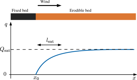
Figure S3: A schematic representation of the saturation length experiment. The saturation length may be described as the relaxation length of the sand flux $q$ toward its saturated value $Q_{\rm sat}$. The experiment set-up is a flat sand bed preceded by a flat non-erodible bed. When the wind blowing over this rigid surface reaches the erodible bed, the sand flux relaxes exponentially towards its saturation value $Q_{\rm sat}$ over a characteristic distance $l_{\rm sat}$ in the direction of the flow.

As shown in Fig. S4 and in Fig. 3 of the main manuscript, we determine the value of $l_{\rm sat}$ from the evolution of the topography of a rectangular sand pile placed downstream of a non-erodible bed composed of gravels. We thus have the experimental setup that best reflects the theoretical conditions presented in Fig. S3. The rectangular sand pile has a length of 12 m and a width of 3 m with its main axis aligned in the northwest-southeast direction, parallel to the orientation of the prevailing wind (Fig. S4a). The initial sand pile was prepared and scanned on April 22, 2014 (Fig. S4b). A storm occurred on April 24 with winds from the north-northwest and irregular wind speeds reaching 15 m s^-1 at a height of 2 m. The sand pile was scanned again on April 25 (Fig. S4c).

Considering the ideal assumption of our initially flat surface under a steady wind of constant direction, strength and transport rate $q$, Eq. 11 can be combined with the equation of conservation of mass to estimate the erosion rate

$$\dfrac{\partial h(x)}{\partial t}=-\dfrac{\partial q(x)}{\partial x}=-\dfrac{Q_{\rm sat}}{l_{\rm sat}}\exp\left(\dfrac{x-x_{0}}{l_{\rm sat}}\right).$$ (13)

This equation can be integrated to estimate the net erosion over a given time period. In this case the exponential regime is expected to hold. However, it cannot be observed from the start of the erodible bed for several reasons, both theoretical and experimental. The main reasons are related to (1) the natural variability of wind speed and direction and (2) the development of a discontinuity in the topographic profile between the non-erodible and the erodible beds. In addition, Eq. 13 neither takes into account the possible dependence of $l_{\rm sat}$ on wind speed[17], nor the spatial shift associated with the establishment of a transport layer when the sand flux starts from zero[16].

Using the field data and despite the number of simplifying assumptions, we study the difference in height $\Delta H$ between the two surface elevations to look for zones where

$$\Delta H\sim-\exp(x/l_{\rm sat}).$$ (14)

In practice, we use 2D elevation profiles aligned with the primary sand transport direction during the storm. It forms an angle of 22° with the orientation of the initial sand pile. This angle is estimated from the sand flux rose as well as from the orientation of ripples and accretion mounds (Fig. S4c).

The slope of the exponential decay in Eq. 14 gives the value of $l_{\rm sat}$ (Fig. 3D of the main manuscript). We find a value of 0.95 m from our field data, a value that can be directly compared to the 0.83 m predicted by Eq. 12 and the parameters given in Tab. S1.

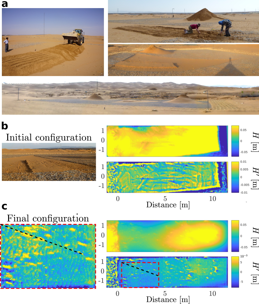
Figure S4: Measuring the saturation length $l_{\rm sat}$ in the field. (a) Setting up the $l_{\rm sat}$ experiment between the two sand piles of the elongating dune experiment in a triangular area of bare sand within a flat bed armored with gravels. In this area, a rectangular sand pile 12 m long and 3 m wide is placed downstream of the non-erodible gravel bed. The long axis is aligned along the northwest-southeast direction, the orientation of the prevailing wind. The sand bed is flattened so that there is no vertical step between the erodible and non-erodible zones. (b) Elevation of the rectangular sand pile on April 22, 2014 before aeolian transport. (c) Elevation of the rectangular sand pile on April 25, 2014 after the passage of a northwestern depression (see flux rose in Fig. 3C of the main manuscript). $H$ is the absolute elevation from a base level. $H^{\prime}$ is the difference of elevation with a smoothed surface obtained using a sliding window with a radius of 20 cm. The inset in c show the transect along which the elevation profile used to estimate $l_{\rm sat}$ has been extracted (see Fig. 3B of the main manuscript). It is parallel to the sand deposits that form downwind of topographic obstacles and perpendicular to aeolian ripples.

5 Supplementary Note 5
Upwind velocity shift at dune crests and troughs

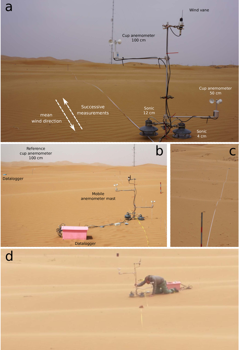
Figure S5: Experimental set-up to estimate the upwind velocity shift at the crests and troughs of incipient dunes. (a) The mobile anemometer mast, with anemometers located at heights of 4 and 12 cm in the inner layer and at heights of 50 and 100 cm in the outer layer. Arrows show the mean wind direction and the measurement path. (b) The anemometer mast and the reference anemometer. (c) A measurement path perpendicular to the crest orientation of the bed instability. (d) Setting a new measurement for 10 min with a sampling frequency of 1 Hz.

5.1 The inner and outer layers

Flows that are topographically forced by obstacles (e.g., hills or sand dunes) accelerates on the upwind slopes and decelerates on the downwind slopes. Then, in order to study sediment transport over a dune, we should first describe some properties of the turbulent flow over an undulating topography. Conceptually, as proposed by Jackson and Hunt (1975)[18] in the limit of small amplitudes bedforms, the turbulent flow over a sinuous bed elevation profile of wavelength $\lambda$ can be decomposed into two layers:

• The outer layer is the external region (supposed infinite) where the pressure gradient set up by the topography is balanced by the inertial forces. The streamlines follow the topography. At a given height, the wind speed is maximum (minimum) above the top (bottom) of the topography. The amplitude of the perturbation vanishes on a characteristic height that varies according to the wavelength of the topography. Then, sufficiently far above the obstacle, the wind speed is finally equal to the undisturbed wind speed in the absence of topography (see Eq. 1).

• The inner layer is a zone in which the longitudinal pressure gradient exerted by the fluid is compensated by the Reynolds shear stress induced by the turbulent motions at the surface of the bed. Then, the pressure gradient is in phase quadrature with the topography and is maximum where the stoss slope is steepest. Hence, there is an upwind velocity shift within the inner layer. The characteristic thickness $l$ of the inner layer depends on both the wavelength of the bed elevation profile and on the aerodynamic roughness $z_{\rm s}$ so that[18, 19]

  $$\dfrac{l}{\lambda}\log^{2}\left(\dfrac{l}{z_{s}}\right)=2\kappa^{2}.$$ (15)

  For typical value of the aerodynamic roughness ($z_{\rm s}<10^{-2}$ m) and wavelengths of hundreds of meters, the inner layer is always confined in a meter scale envelop above the topography. For $\lambda=20\;{\rm m}$ and $z_{\rm s}=10^{-3}\;{\rm m}$, common values observed during the development of aeolian bedforms under high wind speed, the inner layer is less than 20 cm.

5.2 Measuring the upwind velocity shift within the inner layer

A sufficiently strong wind and a stable wind orientation are essential for the quality of the measurements. The sequence of measurements consists in moving an anemoter mast upwind along a given profile of known elevation. The entire procedure to estimate the upwind velocity shift on dunes is described in full details in Claudin et al. (2013)[20]. We follow here the same procedure with the specifications detailed below.

We performed our measurements on low dunes with sinusoidal shape. The density of measurements is high near the crests and troughs ($\approx 20\;{\rm cm}$) but lower in the steeper sections ($\approx 1\;{\rm m}$). Each measurement lasts 10 min with a sampling frequency of 1 Hz. The mobile anemometer mast has sonic anemometers located at heights of 4 and 12 cm and cup anemometers at heights of 50 and 100 cm (Fig. S5a). Given the natural variability in wind speed between two measurements, the wind speeds measured along the mobile mast are normalized by the wind speed measured at one meter high by a reference cup anemometer located at the top of a larger dune in the vicinity (Fig. S5b). The normalized wind speeds along the profile can then reveal how sensitive is the flow to topography at different heights. As shown in Fig. 4B of the main manuscript, in the limit of small sinusoidal oscillations, the wind profiles at all heights reflect the topography, i.e., the spatial variation of the wind speed exhibits the same wavelength as the bedforms. Most importantly for our present purposes, the flow is in phase with the topography at heights of 50 and 100 cm and in phase advance at heights of 4 and 12 cm. It indicates that the inner layer has a thickness between 12 and 50 cm, a range of value that covers entirely the values given by Eq. 15 for aeolian dune systems on Earth.

5.3 From the upwind velocity shift to the hydrodynamic parameters $A$ and $B$

On several occasions during our field campaigns, we have measured wind velocity in the inner and outer layers on a succession of crests and troughs to estimate the phase shift over more than a wavelength of the dune pattern (Fig. S5c,d). Here, we focus only on individual dune crests or troughs, which are approximated by

$$H(x)=H_{\rm ref}+h\cos(kx),$$ (16)

where $k$ is the wave number (wavelength $\lambda=2\pi/k$), $h$ the amplitude. The position of the dune crests and troughs are set at $x=0$ and $x=\lambda/2$, respectively. The arbitrary reference level $H_{\rm ref}$ is here chosen such that $H>0$. Fitting Eq. 16 to the dune elevation data gives the values of $k$ and $h$. The dune aspect ratio is $R=2h/\lambda=hk/\pi$. When the aspect ratio is below $\simeq 0.05$, we expect that the (low) perturbation calculation of the aerodynamics to be valid. A more refined analysis would involve the computation of the Fourier transform of the dune profile, in order to account for a whole range of wave numbers $k$.

Alike topography, the wind profile at a given height along the dune can also be fitted by a sinusoidal function of the same wave number $k$ as for the dune elevation:

$$u_{\rm b}(x)=u_{\rm b}^{0}+\delta u_{\rm b}\cos(kx+\varphi_{\rm b}).$$ (17)

As said in Sec. 5.1, the topography $Z(x)$ and the wind velocity $u_{\rm b}(x)$ are not in phase for anemometers at heights of 4 and 12 cm: the velocity reaches its maximum upstream of the crest. Here the phase difference is $\varphi_{\rm b}$ so that the upwind velocity shift in the inner layer is $\varphi_{\rm b}/k$.The two other fitting parameters are $u_{\rm b}^{0}$ and $\delta u_{\rm b}$.

Because the logarithmic law of the wall (Eq. 1) locally holds in the inner layer at each position $x$, the velocity can be used as a proxy to calculate the basal shear stress with $\tau_{\rm b}\propto\rho_{\rm f}u_{\rm b}^{2}$. By expansion to the first order, we can then write:

$$\tau_{\rm b}(x)\propto\rho_{\rm f}(u_{\rm b}^{0})^{2}\left(1+kh\left(A\cos(kx)-B\sin(kx)\right)\right),$$ (18)

where $A$ and $B$ are given by

$$A=2\times\frac{\delta u_{\rm b}}{u_{\rm b}^{0}}\times\dfrac{\cos(\varphi_{\rm b})}{kh}\;\;\;\;\;\;\;\;\;\;\;\;\;\;\;\mbox{and}\;\;\;\;\;\;\;\;\;\;\;\;\;\;\;B=2\times\frac{\delta u_{\rm b}}{u_{\rm b}^{0}}\times\dfrac{\sin(\varphi_{\rm b})}{kh}\,.$$ (19)

Eqs. 18 and 19 are specific to the quadratic relation between $\tau_{\rm b}$ to $u_{\rm b}$. Since sediment transport is controlled by the basal shear stress, these two parameters $A$ and $B$ are all that are needed as aerodynamical inputs in bedform evolution models. As described in the introduction of the main manuscript, they are of fundamental importance for the understanding of the mechanisms of dune growth and dune size-election (see also Sec. 6 and Eqs. 23-24). Tab. S2 shows the results obtained in April and November 2015 in our experiment. We observe no significant trend in the variation of $A$ and $B$ during dune growth.

Variable		Units		Description
Topography
$\lambda$		m-1		dune wavelength
$k$		m-1		Dune wave number
$h$		m-1		Amplitude of the dune
$R$		$\emptyset$		Dune aspect ratio
Flow
$\delta u_{\rm b}$		${\rm m\;s}^{-1}$		Amplitude of wind speed variation in the inner layer.
$u_{\rm b}^{0}$		${\rm m\;s}^{-1}$		Mean wind speed in the inner layer.
$\varphi_{\rm b}$		o		Phase shift between the flow and the topography in the inner layer.
Hydrodynamic parameters
$A$		$\emptyset$		In-phase hydrodynamic parameter
$B$		$\emptyset$		In-quadrature hydrodynamic parameter

	14/04	15/04	15/04∗	15/04	16/04	18/04	03/11	03/11∗	03/11	15/11
Topography
$\lambda$	14.84	18.57	10.50	16.45	21.92	14.51	25.05	14.49	21.06	14.33
$k$	0.423	0.338	0.598	0.382	0.287	0.433	0.251	0.437	0.298	0.439
$h$	0.297	0.262	0.185	0.414	0.358	0.338	0.662	0.323	0.264	0.361
$R$	0.020	0.014	0.018	0.025	0.016	0.023	0.026	0.022	0.012	0.025
Flow
$\delta u_{\rm b}$	0.126	0.111	0.108	0.198	0.0624	0.143	0.306	0.134	0.132	0.174
$u_{\rm b}^{0}$	0.683	0.650	0.656	0.678	0.743	0.701	0.568	0.622	0.739	0.661
$\varphi_{\rm b}$	25.51	11.89	15.95	20.79	45.95	10.92	11.36	19.13	17.42	9.80
Hydrodynamic parameters
$A$	2.648	3.770	2.860	3.453	1.138	2.737	6.362	2.906	4.328	3.278
$B$	1.264	0.794	0.817	1.311	1.176	0.528	1.278	1.008	1.358	0.566

Table S2: Topography and wind measurements carried out in April and November 2015. Measurements on dune troughs are shown with a ^∗ on April 4 and November 3, 2015. They are located between two dune crests along the same transect to estimate the phase shift over more than one wavelength of the dune pattern.

6 Supplementary Note 6
Dispersion diagram from successive topographic surveys

Dispersion relations are plotted as growth rate $\sigma$ and phase velocity $c$ with respect to wave number $k$. They are used in linear stability analysis to identify the most unstable wavelength, which is likely to be observed. We describe here how we measure the growth rate of dunes as a function of their wave numbers $k$ from successive topographic surveys throughout the duration of our experiment. Before, we present the rational for studying dune formation as a linear instability in a landscape scale experiment.

6.1 Aeolian dune formation as a linear instability

In what follows, the term instability characterizes the growth of a small perturbation in a system, which is often considered to be as homogeneous and simple as possible. Conversely, stability refers to the ability of this system to return to its original state when perturbed. The main objective of stability analysis is to identify the ranges of perturbation wavelengths over which the system exhibits stable or unstable behavior. Quantitative approaches consists of estimating the initial growth rate of each mode (wavelength) considering that all these modes are independent of each other. Obviously, the highest and zero growth rates are particularly important. The highest ones are associated with the most unstable modes, which will have the greatest impact on the system. Those at zero are neutral modes that often mark the transition between stable and unstable regimes.

The analysis of the time and length scales of instabilities by means of linearized equations is a standard approach in hydrodynamics and many other branches of physics. By identifying stabilizing and destabilizing mechanisms, these linear stability analysis reveal how they together govern the the evolution of the system over the entire range of possible wavelengths. During the first stage of the instability (the linear regime), the initial wavelength $\lambda_{\rm g}$ of the perturbation is assumed to stay constant, whereas its amplitude $h$ grows exponentially with time

$$h(k_{\rm g},t)\propto\exp(\sigma(k_{\rm g})t).$$ (20)

In this expression, $k_{\rm g}=2\pi/\lambda_{\rm g}$ is the wave number and $\sigma(k_{\rm g})$ the growth rate with units of frequency. Positive and negative growth rates correspond to unstable and stable modes, respectively. The dispersion relation $\sigma(k)$ gives the growth rate value of the perturbation as a function of the wave number $k$. The largest positive $\sigma$-value corresponds to the most unstable mode $\{k_{\rm max},\,\lambda_{\rm max}\}$. Zero values corresponds to neutral modes $\{k_{0},\,\lambda_{0}\}$. In diffusive systems, dispersion relations are often characterized by a transition from a stable to an unstable regime. for an increasing wavelength. In other words, $\sigma(k)>0$ for $k<k_{0}$ and $\sigma(k)<0$ for $k>k_{0}$. Beyond the linear stage of the instability, when the amplitude of the initial perturbation is too high, the dispersion relation no longer applies because the different modes interact with one another. It is described as the non-linear stage of the instability.

Here, we study the formation of aeolian dunes as a linear instability. More exactly, we focus on the dependence and feedback between bed forms, wind flow and sand transport properties. The governing equations lead to the theoretical expression of a dispersion relation as a function of the different physical parameters of the system (see Eq. 1 of the main manuscript). Thus, the minimum size for dunes is associated with a neutral mode and a transition from unstable to stable regime for decreasing wavelength. The emergence and growth of periodic dune patterns are associated with a most unstable mode which is going to prevail within the whole dune field. Based on observation of mature aeolian dunes in nature, previous studies have measured the wavelength and the migration rate of dunes in order to derive values of $\lambda_{0}$, $\lambda_{\rm max}$ and $\sigma_{\rm max}$ under various conditions. Dispersion relations have been given less attention or even disregarded, certainly because of the length and time scales involved in the mechanism of aeolian dune growth. Then, a direct validation of the dune instability theory is to investigate whether or not dispersion diagrams can be derived from field data. Another solution is to verify whether the theoretical formalism used with the values of the underlying physical parameters measured independently in the field is actually capable of accurately predicting the observations.

Here, we apply this methodology to the formation of dunes in a landscape scale experiment. Our initial system is a sand bed after flattening by a bulldozer. In such an experimental set up, but also in all natural dune environments, there are always heterogeneities and defects at all length scales and our initial condition already contains all the perturbation wavelengths.

6.2 The transition from the linear to the non-linear phases of dune growth

The continuous transition from the linear to the non-linear phases of dune growth is controlled by dune aspect-ratio, which is the main control parameter for aerodynamic non-linearities. Figs. S6a-b show the elevation and slope maps during incipient dune growth in our experimental field from April 10, 2014 to July 6, 2015. There is a significant change in slope maps between October 30 and November 12, 2014. Over this time interval, the local slopes not only become steeper, they also become spatially organized, just like dune crest, to form more regular transverse structures across the flattened area. This occurs for a mean slope of about 0.03 (Fig. S6c) at the same time as incipient slip faces a few centimeter high emerge (Fig. S7). The mean slope $\langle\|\vec{\nabla}H\|\rangle$ variations can be compared to the amplitude of the bedforms in Figs. S6b-c. Based on these observations, we set the transition between October 30 and November 12, 2014. This transition is not spontaneous but it is surely completed in April 2015, when the mean slope reaches a value of about 0.07.

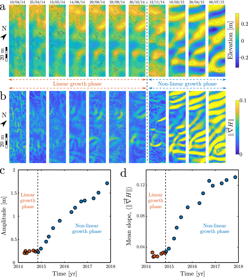
Figure S6: The transition from the linear to the non-linear phases of dune growth. (a) Elevation and (b) slope maps during incipient dune growth from April 10, 2014 to July 6, 2015. The colormap in Fig. S6b is saturated to distinguish the slopes of bedforms in fall 2014, around the transition from the linear to the non-linear phases of dune growth. In non-saturated areas, ripples can be observed. A cable crosses the experimental field from 28 April 2015. (c) The mean amplitude $2\sqrt{2}(\langle h^{2}\rangle-\langle h\rangle^{2})^{1/2}$ of bedforms and (d) the mean slope $\langle\|\vec{\nabla}H\|\rangle$ with respect to time. The higher mean slope value on April 10, 2014, after the flattening, is due to bulldozer tracks that can be seen in Fig.S6b. Colors and dashed lines are used to separate the linear (orange) and the non-linear (blue) phases of dune growth. For comparison with slope data, Fig. S6d is the same as Fig. 5C of the main manuscript.

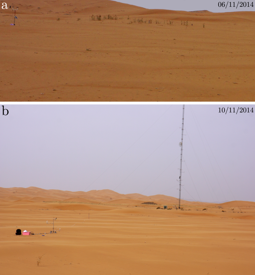
Figure S7: Bedforms during the transition from the linear to the non-linear phases of dune growth. (a) Incipient slip faces a few centimetres high on November 6, 2014. (b) Periodic dune patterns on November 10, 2014. This pictures can be compared to elevation and slope maps of October 30, 2014 and November 12, 2014 shown in Fig. S6a and S6b.

6.3 A transport time scale for dune growth under variable wind strength

In order to quantify dune growth under variable wind strength, it is necessary to define a new time scale that accounts for the intensity of transport. For example, periods during which there is no transport should not be used as time increments, while storm periods should contribute more to the total time.

In practice, the new time scale is defined sequentially from the wind data using the saturated sand flux (Eq. 3) and the saturation length $l_{\rm sat}$. Starting at $t=0$ at the flattening time, the new times write

$$t_{\rm a}(t)=\dfrac{\displaystyle\sum_{i=1}^{t}\|\overrightarrow{Q_{i}}\|\delta t_{i}}{l_{\rm sat}^{2}}.$$ (21)

This time scale is dimensionless allowing for comparison across different time series and various time periods. Using the saturated sand flux derived from the local wind data (Eq. 3), Fig. S8 shows the dimensionless times with respect to time from April 10, 2014 to October 31, 2017 using the saturation length $l_{\rm sat}=0.95\leavevmode\nobreak\ {\rm m}$ measured in the field (Fig. 3 of the main manuscript). By definition, periods of stronger winds are associated with steeper slopes, and vice versa. The choice of the characteristic length for the computation of the dimensionless transport time scale, (here $l_{\rm sat}$) is of minor significance since we consider it to be constant.

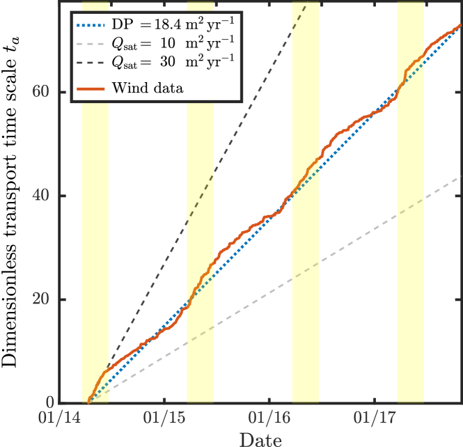
Figure S8: A dimensionless transport time scale for dune growth under variable wind strength. Using the saturated sand flux derived from wind data (Eq. 3), the red solid line shows the dimensionless transport time scale $t_{a}$ as a function of time from April 10, 2014, when the dune field was flattened. By definition, the mean slope is given by the RDP (blue line, Eq. 5). Light and dark gray lines show the transport time scale for constant sand fluxes of 10 and 30 ${\rm m}^{2}\,{\rm yr}^{-1}$, respectively. Highlighted areas show the spring periods from March 21 to June 21.

6.4 Topographic surveys during experimental dune growth

From April 2014 to November 2017, we performed a series of topographic surveys of the dunes developing from the flat sand bed using a ground-based laser scanner Leica Scanstation C10 (Fig. S9a). To compare these different measurements, a reference system of concrete posts was installed over the entire experimental dune field (Figs. S9b-d). For each survey, the zone under investigation is scanned from four different view points. Over the 42 months of the experiment, the density of points varies from 472 to 2368 points/m².

To map surface elevation, we select only elevation points within the 4-sided polygon determined by reference points t6, t7, t8 and t9 (Figs. S9c-d). Within this polygon, to avoid disturbances from the surrounding bedforms, we have chosen a central rectangular area with a width of 48 m and a length of 82 m (ABCD in Figs. S9c-d). The long side of this rectangle is oriented Northwest-Southeast to align perpendicular to the final orientation of the dunes at the end of the experiment. We remove the mean slope of this rectangular area by adjusting a plane to the elevation data. This plane has always a southwest-facing slope during the entire duration of the experiment. The residual topography is shown for different times in Fig. 5A of the main manuscript. Within the rectangular area, we study 2D transects parallel to the main axis using a spacing of 1.4 m between two transects (see for example transect $aa^{\prime}$ in Figs. S9c-d). For each of the 34 transects, we select the elevation data points in a 0.2 m wide band on either side. All these points are horizontally projected on their respective transect line. After substracting the average slope and the mean elevation, we resample these data to a regular spacing of 0.1, 0.25 and 0.35 m. Thus, we can use the fast Fourier transform method to explore different values within the frequency domain.

Fig. 5B of the main manuscript shows the elevation profiles with respect to time for the transect $aa^{\prime}$ shown in Figs. S9c-d. Over the 42 months of the experiment, the amplitude of the dunes varies from a few centimeters to a few meters.

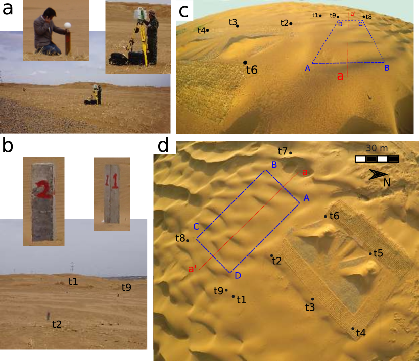
Figure S9: Topographic surveys during experimental dune growth. (a) Ground laser scanning in the landscape-scale experiment. (b) Ground view of three posts of the local reference system. (c,d) Reference system (dots) and selected area (blue rectangle) for the entire duration of the experiment. All 2D elevation profiles are taken parallel to the transect $aa^{\prime}$ (red line). They are separated by a distance of 1.4 m. The elevation profiles of the same transects at different times are used to study the dune instability.

6.5 Spectral analysis, amplitude and phase

For each transect and all topographic surveys, we use a fast Fourier transform method to analyze the signal in the frequency domain (Figs. S10a,b). By selecting only one frequency value, the individual contribution of each wavelength is computed by an inverse Fourier transform (Fig. S10c). Thus, we obtain a sine wave

$$H_{\lambda_{i}}^{j}(t_{n})=h_{\lambda_{i}}^{j}(t_{n})\cos(k_{i}x+\phi^{j}_{\lambda_{i}}(t_{n}))$$ (22)

for each wavelength $\lambda_{i}=2\pi/k_{i}$ of each transect $j$ at the different times $t_{n}$ of the $n^{\rm th}$ topographic survey. Considering the 34 different transects, the amplitude $h$ and the phase $\phi$ can be used to estimate growth rates $\sigma_{\lambda_{i}}$ and phase velocities $c_{\lambda_{i}}$ with respect to time, respectively. We perform this analysis on the same elevation profiles sampled at different rates (0.1, 0.25 and 0.35 m) to verify that it has no effect on the spectral behavior.

Taking as an example transect N^o 20 in the middle of the selected area, Fig. S11 shows the logarithm of the amplitude $A_{\lambda}^{20}$ of individual wavelengths with respect to the dimensionless time scale. A sudden change in behavior is observed between $t_{a}=10.7$ and $t_{a}=11.3$, i.e. from October 30 to November 12, 2014. Over this time period, there is an abrupt increase in growth rate and then a more irregular behavior than during the initial phase. As shown in Fig. 5C of the main manuscript, it is also during this period that the mean amplitude of the bedforms begins to increase more rapidly. These behaviors are interpreted as the transition between linear and non-linear growth phases. This interpretation is supported by the observation of the first slip faces downwind of the crest under the prevailing wind.

In order to quantify dune growth in the linear phase according to the dune instability (see Sec. 6.1 and Eq. 20), we perform an exponential fit to the amplitude data from $t_{a}=0$ to $t_{a}=10.7$, i.e. from April 10 to October 30, 2014, for each wavelength and each transect (see red lines in Fig. S11). The agreement between the exponential regime and the data as well as the variation of the exponential rate at different wavelengths indicate that there is a coherent behavior at different length scales, which can be analyzed thanks to a dispersion diagram.

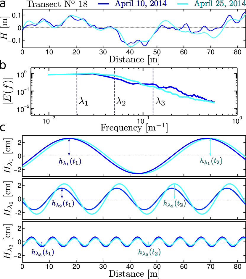
Figure S10: Spectral analysis of elevation profiles with respect to time. (a) Two consecutive elevation profiles of transect N^o 18 during dune growth. (b) Power spectral density of the elevation profiles using a fast Fourier transform. Dashed lines show wavelengths $\lambda_{\{1,2,3\}}$ of $\{51.2,\,20.5,\,7.9\}$ m. (c) The reconstructed elevation profiles using individual wavelengths $\lambda_{\{1,2,3\}}$ and the inverse Fourier transform. By definition, they take the form of sine waves $H_{\lambda_{i}}=h_{\lambda_{i}}\cos(k_{i}x+\phi_{\lambda_{i}})$ where $k_{i}=2\pi/\lambda_{i}$ is the wave number and $\phi_{\lambda_{i}}$ the phase. Values of $h_{\lambda_{i}}$ and $\phi_{\lambda_{i}}$ at different times can be used to estimate growth rate $\sigma_{\lambda_{i}}$ and phase velocity $c_{\lambda_{i}}$, respectively.

6.6 Dispersion diagram of the growth rate

Fig. S11 shows the dispersion relation for transect N^o20 during the linear phase from $t_{a}=0$ to $t_{a}=10.7$, i,e. from April 10 to October 30, 2014. In this figure, the exponential rates of growth or decay of the different wavelengths $\lambda_{i}$ are plotted with respect to the wave number $k_{i}=2\pi/\lambda_{i}$. From the longest wavelengths (i.e. smallest wave numbers), there is an increase in the growth rate. The maximum growth rate is reached for $k_{\rm max}\approx 0.43\leavevmode\nobreak\ {\rm m}^{-1}$ ($\lambda_{\rm max}\approx 14.6\leavevmode\nobreak\ {\rm m}$). For shorter wavelengths, the growth rate is decreasing and the neutral mode is reached for a value of $k_{0}$ of about $0.67\leavevmode\nobreak\ {\rm m}^{-1}$ ($\lambda_{\rm c}\approx 9.3\leavevmode\nobreak\ {\rm m}$). Then, shorter wavelengths have negative growth rates. These decay rates are associated with small amplitudes of less than one centimeter, so that their rapid variations can not be captured given the resolution of our topographic data.

Fig. S12a shows the dispersion relations of the growth rate for all transects and the three sampling rates. The mean and standard deviation of these growth rates are plotted with respect to the wave number in Fig. S12b. Using these data, we find $k_{\rm max}\approx 0.45\leavevmode\nobreak\ {\rm m}^{-1}$ ($\lambda_{\rm max}\approx 14\leavevmode\nobreak\ {\rm m}$) and $k_{\rm c}\approx 0.7\leavevmode\nobreak\ {\rm m}^{-1}$ ($\lambda_{\rm c}\approx 9\leavevmode\nobreak\ {\rm m}$).

Theoretically, the growth rate writes

$$\sigma(k)=Q\,k^{2}\,\dfrac{B-A\,k\,l_{\rm sat}}{1+\left(k\,l_{\rm sat}\right)^{2}}$$ (23)

where $A$ and $B$ are the aerodynamic parameters (Sec. 5), $l_{\rm sat}$ the saturation length (Sec. 4), $Q$ a constant flux proportional to $u_{*}^{2}$. This equation does not take into account the transport threshold and is therefore theoretically valid only within the limit of strong winds when the sand flux is large. However, the role of the transport threshold is included in our estimates thanks to the dimensionless time scale and a prefactor correcting for the intensity of the sand flux. In practice, the growth rate derived from the elevation profiles scales as $\sigma(k)/Q$ and we consider a prefactor $\langle u_{*}\rangle^{2}/(\langle u_{*}\rangle^{2}-u_{\rm th}^{2})$ that integrates all the variations of wind strength. Thus, the parameter $A$ and $B$ in Eq. 18 and in Eq. 23 are compatible with one another.

The dispersion relation using Eq. 23 and the values of $\{l_{\rm sat},\,A,\,B\}=\{0.95,\,3,\,1.5\}$ measured independently in the field are plotted in orange in Figs S11 and S12 as in Fig. 6B of the main manuscript. The blue curve in these figures corresponds to a dispersion relation with the best-fit values of $\{l_{\rm sat},\,A,\,B\}=\{0.7,\,1.96,\,0.96\}$. In addition, to investigate the sensitivity of the dispersion relation to the values of $\{l_{\rm sat},\,A,\,B\}$, the shaded area in Fig. 3c of the main manuscript shows the best-fit values of $A$ and $B$ using values of $l_{\rm sat}\in[0.5;\,1.1]$ in Eq. 23. All these results underline the consistency of the experimental dispersion diagram derived from the topographic data not only with the theory but also with our independent measurements of flow and transport properties in the field.

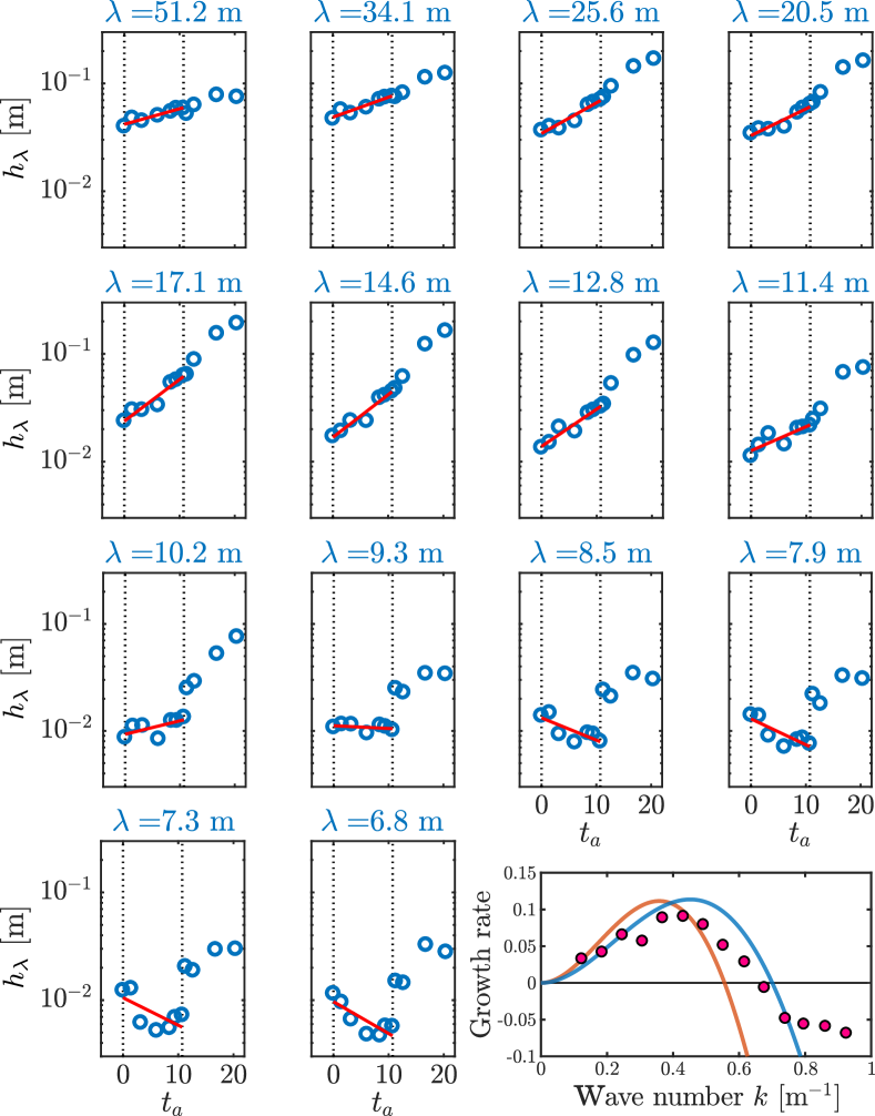
Figure S11: Growth rate of individual wavelengths. Considering the elevation profiles of transect N^o20 and a sampling rate of 25 cm, figures show the logarithm of the amplitude $h_{\lambda}$ of individual wavelengths with respect to the dimensionless time scale; $t_{a}=0$ is set for April 10, 2014. Two different regimes are observed before and after $t_{a}=10.7$, November 30, 2014. There are associated with the linear and non-linear growth phases. The growth rate of each wavelength is determined by an exponential fit performed during the linear phase ($0\leq t_{a}\leq 10.7$, dashed lines). As a synthesis, the bottom right figure shows the dispersion relation, i.e. the growth rate with respect to the wave number $k=2\pi/\lambda$. Solid lines are the same dispersion relations as in Fig. 6B of the main manuscript: $\{l_{\rm sat},\,A,\,B\}=\{0.95,\,3,\,1.5\}$ (orange) and $\{0.7,\,1.96,\,0.96\}$ (blue). Note that small wavelengths have amplitude of less than one centimeter. These amplitudes are comparable to the noise level of our topographic measurements, which prevents the estimation of the exponential decrease in growth rate for short wavelengths ($\leq$ 8 m).

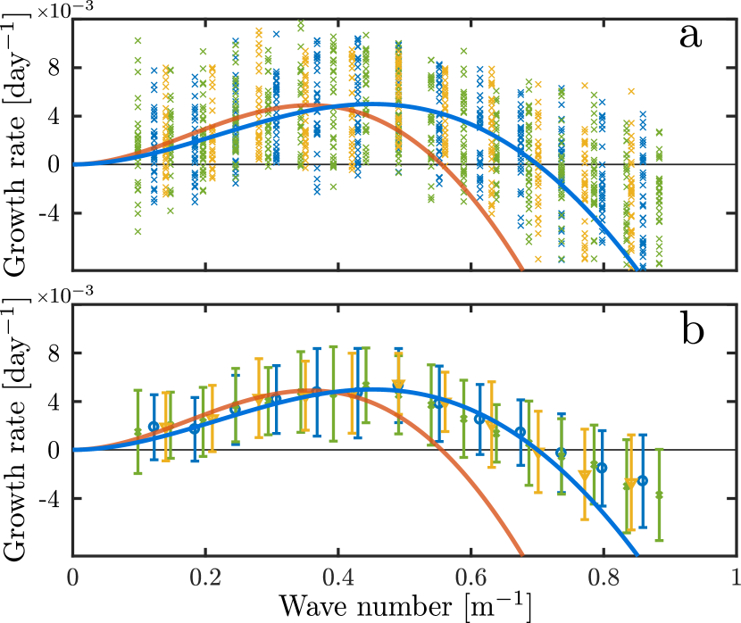
Figure S12: Dispersion diagram of the growth rate for all transects at different sampling rates. (a) Growth rates during the linear phase, i.e. from April 10, 2014 to November 30, 2014, with respect to the wave number $k=2\pi/\lambda$ for each transect and sampling rates of 0.1 m (blue), 0.25 m (yellow) and 0.35 m (green). (b) Mean and standard deviation of the growth rates averaged on all transects. Solid lines are the same dispersion relations as in Fig. 6B of the main manuscript and in Fig. S11: $\{l_{\rm sat},\,A,\,B\}=\{0.95,\,3,\,1.5\}$ (orange) and $\{0.7,\,1.96,\,0.96\}$ (blue).

6.7 Dispersion diagram of the phase velocity

During the linear-growth phase, the analysis of the variation of the phase $\phi(\lambda_{i})$ (Eq. 22) as a function of time do not at present provide conclusive evidence about the dispersion diagram of the phase velocity. An obvious limitation comes from the time delay between two consecutive topographic surveys. Indeed, the phase shift can be too large to be accurately computed, even by folding the data modulo the period from large to short wavelengths. The orientation and magnitude of the resultant sand flux associated with each time interval is another obvious issue. In fact, wind reversals and the subsequent back and forth of the incipient bedforms were frequent during the experiment. Variation of the phase data during periods of strong winds and small resultant sand flux are particularly difficult to be interpreted.

To simplify the problem, we can also estimate dune migration distance by cross correlation between two elevation profiles over a time interval over which the wind is almost unidirectional, from April 25 to May 13, 2014, (Figs. S13a,b). The dune migration rate can then be computed using the dimensionless time scale to be compared to theoretical dispersion relations. With the same notation as in Eq. 23, dispersion relations write

$$c(k)=Q\,k\,\dfrac{A+B\,k\,l_{\rm sat}}{1+\left(k\,l_{\rm sat}\right)^{2}}.$$ (24)

Considering the dimensionless time scale and the same prefactor as for the growth rate, Fig. S13c shows the dispersion relations of the phase velocity using the same parameters as in Figs. S11 and S12. It also shows the phase velocity of the most unstable wavelength $\lambda_{\rm max}$, the mean value of the migration rate averaged over all transects and the corresponding standard deviation. As expected, the migration rate derived from the cross correlation is close to the phase velocity of the most unstable wavelength.

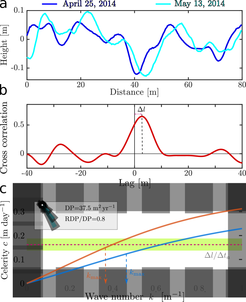
Figure S13: Dispersion diagram of the phase velocity. (a) Two consecutive elevation profiles of transect N^o 16 during dune growth. (b) The maximum value of the cross correlation diagram between the two elevation profiles determines the dune migration distance $\Delta l=3.25\leavevmode\nobreak\ {\rm m}$ from April 25 to May 13, 2014 (i.e. $\Delta t_{a}=1.77$). (c) Dispersion diagram of the phase velocity using the same parameters as in Fig. 6B of the main manuscript and in Figs. S11 and S12b: $\{l_{\rm sat},\,A,\,B\}=\{0.95,\,3,\,1.5\}$ (orange) and $\{0.7,\,1.96,\,0.96\}$ (blue). Vertical dashed lines show the most unstable wavelength $\lambda_{\rm max}$ in both cases. Using cross correlation, the horizontal dashed lines shows the mean migration velocity $\Delta l/\Delta t_{a}$ averaged over all transects. The shaded area has a width of two standard deviation using the same data. There is a quantitative agreement between $c(\lambda_{\rm max})$ and the migration rate derived from $\Delta l/\Delta t_{a}$. This is possible because during this period of time of the linear growth phase the wind regime is almost unidirectional (see inset).

References

- [1] Iversen, J. D. & Rasmussen, K. R. The effect of wind speed and bed slope on sand transport. Sedimentology 46, 723–731 (1999).
- [2] Ungar, J. & Haff, P. Steady state saltation in air. Sedimentology 34, 289–299 (1987).
- [3] Durán, O., Claudin, P. & Andreotti, B. On aeolian transport: Grain-scale interactions, dynamical mechanisms and scaling laws. Aeolian Research 3, 243–270 (2011).
- [4] Fryberger, S. G. & Dean, G. Dune forms and wind regime. A study of global sand seas 1052, 137–169 (1979).
- [5] Pearce, K. I. & Walker, I. J. Frequency and magnitude biases in the ‘Fryberger’ model, with implications for characterizing geomorphically effective winds. Geomorphology 68, 39–55 (2005).
- [6] Tsoar, H. Sand dunes mobility and stability in relation to climate. Physica A 357, 50–56 (2005).
- [7] Bagnold, R. The physics of wind blown sand and desert dunes: London (1941).
- [8] Sauermann, G., Kroy, K. & Herrmann, H. J. Continuum saltation model for sand dunes. Physical Review E 6403, art. no.–031305 (2001).
- [9] Narteau, C., Zhang, D., Rozier, O. & Claudin, P. Setting the length and time scales of a cellular automaton dune model from the analysis of superimposed bed forms. J. Geophys. Res. 114 (2009).
- [10] Andreotti, B., Claudin, P. & Douady, S. Selection of dune shapes and velocities: Part 1: Dynamics of sand, wind and barchans. Eur. Phys. J. B 28, 321–339 (2002).
- [11] Charru, F. Selection of the ripple length on a granular bed. Phys. Fluids 18, 121–508 (2006).
- [12] Elbelrhiti, H., Claudin, P. & Andreotti, B. Field evidence for surface-wave-induced instability of sand dunes. Nature 437, 720–723 (2005).
- [13] Fourrière, A., Claudin, P. & Andreotti, B. Bedforms in a turbulent stream: formation of ripples by primary linear instability and of dunes by nonlinear pattern coarsening. Journal of Fluid Mechanics 649, 287–328 (2010).
- [14] Hersen, P., Douady, S. & Andreotti, B. Relevant length scale of barchan dunes. Physical Review Letters 89 (2002).
- [15] Andreotti, B. The song of dunes as a wave-particle mode locking. Physical Review Letters 93 (2004).
- [16] Andreotti, B., Claudin, P. & Pouliquen, O. Measurements of the aeolian sand transport saturation length. Geomorphology 123, 343–348 (2010).
- [17] Pähtz, T., Kok, J. F., Parteli, E. J. & Herrmann, H. J. Flux saturation length of sediment transport. Physical review letters 111, 218002 (2013).
- [18] Jackson, P. & Hunt, J. Turbulent wind flow over a low hill. Q. J. R. Meteorol. Soc. 101, 929–955 (1975).
- [19] Sykes, R. I. An asymptotic theory of incompressible turbulent boundary layer flow over a small hump. Journal of Fluid Mechanics 101, 647–670 (1980).
- [20] Claudin, P., Wiggs, G. & Andreotti, B. Field evidence for the upwind velocity shift at the crest of low dunes. Boundary-layer meteorology 148, 195–206 (2013).