Exact quench dynamics of symmetry resolved entanglement in a free fermion chain

Abstract

The study of the entanglement dynamics plays a fundamental role in understanding the behaviour of many-body quantum systems out of equilibrium. In the presence of a globally conserved charge, further insights are provided by the knowledge of the resolution of entanglement in the various symmetry sectors. Here, we carry on the program we initiated in [Phys. Rev. B 103, L041104 (2021)], for the study of the time evolution of the symmetry resolved entanglement in free fermion systems. We complete and extend our derivations also by defining and quantifying a symmetry resolved mutual information. The entanglement entropies display a time delay that depends on the charge sector that we characterise exactly. Both entanglement entropies and mutual information show effective equipartition in the scaling limit of large time and subsystem size. Furthermore, we argue that the behaviour of the charged entropies can be quantitatively understood in the framework of the quasiparticle picture for the spreading of entanglement, and hence we expect that a proper adaptation of our results should apply to a large class of integrable systems. We also find that the number entropy grows logarithmically with time before saturating to a value proportional to the logarithm of the subsystem size.

1 Introduction

Understanding the dynamics of entanglement in out-of-equilibrium quantum many-body systems is a prominent challenge in many problems of contemporary physics, such as the equilibration and thermalisation of isolated many-body systems [1, 2, 3, 4, 5], the emergence of thermodynamics in quantum systems [6, 7, 8, 9] or the effectiveness of classical computers to simulate quantum dynamics [10, 11, 12, 13, 14].

Let us consider a system in a pure state $|\psi\rangle$ described by the density matrix $\rho=|\psi\rangle\langle\psi|$. The entanglement between a subsystem $A$ and its complement $B$, is encoded in the reduced density matrix $\rho_{A}$ of system $A$, defined as $\rho_{A}=\text{Tr}_{B}\rho$. The Rényi entropies are entanglement measures labelled by a parameter $n$ (which is integer in the replica approach [15]), and are defined as

$$S_{n}\equiv\frac{1}{1-n}\log\text{Tr}\rho_{A}^{n}.$$ (1.1)

The knowledge of the Rényi entropies for all $n>0$ gives access to the full spectrum of $\rho_{A}$ [16]. The limit $n\to 1$ of Eq. (1.1) defines the entanglement entropy $S_{1}$. It is the von Neumann entropy of the reduced density matrix of system $A$, i.e.

$$S_{1}\equiv\lim_{n\to 1}S_{n}=-\text{Tr}\rho_{A}\log\rho_{A}.$$ (1.2)

The entanglement entropy, and more generally the Rényi entropies $S_{n}$, quantify the entanglement between a subsystem $A$ and its complement. This is independent of the topology of $A$. For example, when $A$ consists of two or more disconnected subsets, $S_{n}$ is still a measure of entanglement between $A$ and the remainder. However, by no means does $S_{n}$ quantify the entanglement between two subsets of $A$. It can anyway be used to construct a measure of the total correlations between the subsets. Let us denote two subsystems $A_{1}$ and $A_{2}$ with $A=A_{1}\cup A_{2}$. The mutual information

$$I_{1}^{A_{1}:A_{2}}\equiv S_{1}^{A_{1}}+S_{1}^{A_{2}}-S_{1}^{A_{1}\cup A_{2}},$$ (1.3)

is a very useful measure of the total correlation between $A_{1}$ and $A_{2}$ [17]. This definition can readily be generalised to a Rényi mutual information

$$I_{n}^{A_{1}:A_{2}}=S^{A_{1}}_{n}+S^{A_{2}}_{n}-S^{A_{1}\cup A_{2}}_{n}=\frac{1}{n-1}\log\left(\frac{\text{Tr}\rho_{A_{1}\cup A_{2}}^{n}}{\text{Tr}\rho_{A_{1}}^{n}\text{Tr}\rho_{A_{2}}^{n}}\right).$$ (1.4)

However, as a very important difference compared to the von Neumann mutual information (1.3), the Rényi one is not a measure of the correlations (e.g., it can be negative for some states [18]). The definition of a proper and calculable Rényi mutual information is a long standing problem, see, e.g., the discussion in the very recent manuscript [19]. We mention that a proper measure to quantify the entanglement between non-complementary subsystems is instead the entanglement negativity [20], that is much more difficult to deal with, especially out of equilibrium [21, 22, 23, 24, 25, 26, 27], and will be investigated in a forthcoming publication [28].

The last decade witnessed an intense theoretical effort aimed at better understanding the dynamics of quantum many-body systems after a quantum quench, the simplest and most broadly studied protocol to drive a quantum system out of equilibrium [29, 30]. In integrable systems, the entanglement dynamics after a quench is well described and understood in terms of the quasiparticle picture [31, 32, 33, 34]. These intense theoretical progress moved together with groundbreaking cold-atom and ion-trap experiments. Most notably, it has been possible to measure the many-body entanglement of non-equilibrium states [35, 36, 37, 38]. In particular, in the experimental paper [36], the authors pointed out that a refined understanding of how the entanglement arises from the various symmetry sectors is necessary to better grasp the full many-body dynamics. Even though the study of the symmetry resolution of entanglement became a very active research area of the last years [39, 40, 42, 43, 49, 45, 50, 41, 46, 51, 44, 52, 53, 55, 56, 57, 58, 59, 60, 62, 66, 54, 63, 65, 61, 70, 64, 67, 68, 69], only few results are available for out-of-equilibrium situations [46, 45, 63, 64], see also [47, 48] as earlier works on the charged moments.

This article is a completion and an extension of our initial Letter [45]. On the one hand, we report many details of calculations in a system of free fermions after a global quantum quench that were only sketched in Ref. [45] due to the lack of space. On the other hand, we also present various new results that we obtained in the meantime, in particular concerning a proposal for the definition of a symmetry resolved mutual information and for the number entropy. We focus on exact lattice calculations for two distinct quenches and compare our results with the quasiparticle picture predictions.

This paper is organised as follows. In Sec. 2 we provide the definitions of the symmetry resolved entanglement entropies and mutual information. We then introduce the model of free fermions that we consider in Sec. 3. Sections 4 and 5 are devoted to the analytical study of the dynamics of the symmetry resolved quantities after a quench from two distinct initial states: the Néel state and the Majumdar-Ghosh dimer state, respectively. In Sec. 6 we give an interpretation of our results in the framework of the quasiparticle picture for the dynamics of entanglement in integrable models. Finally, we give a summary of the results and future outlook of this work in Sec. 7.

2 Symmetry resolution and flux insertion

In this section we give the general definitions of the main quantities of interest, namely the symmetry resolved entanglement entropies and mutual information. We consider an extended quantum system with an internal $U(1)$ symmetry generated by a local operator $Q$. If the symmetry is not broken, we have $[\rho,Q]=0$. For a bipartition in two complementary subsystems $A$ and $B$, by locality the charge $Q$ splits as sum of operators that act on the degrees of freedom of the two parts, $Q=Q_{A}+Q_{B}$. Hence, the trace over the degrees of freedom of subsystem $B$ in the commutation relation $[\rho,Q]=0$ yields $[\rho_{A},Q_{A}]=0$. This relation implies that the reduced density matrix $\rho_{A}$ acquires a block diagonal form, where each block corresponds to a given eigenvalue $q$ of $Q_{A}$. We thus have

$$\rho_{A}=\oplus_{q}\Pi_{q}\rho_{A}=\oplus_{q}[p(q)\rho_{A}(q)]$$ (2.1)

where $\Pi_{q}$ is the projector on the eigenspace of the eigenvalue $q$ and $p(q)=\text{Tr}\left(\Pi_{q}\rho_{A}\right)$ is the probability that a measurement of $Q_{A}$ gives $q$ as outcome. The reduced density matrix in the sector $q$ is normalised so that $\text{Tr}{\rho_{A}}(q)=1$.

2.1 Symmetry resolved entropies

The block structure of the reduced density matrix induces a decomposition of the entropy into contributions associated to each charge sector. For example, plugging Eq. (2.1) into the definition of the von Neumann entropy (1.2), we obtain

$$S_{1}=\sum_{q}p(q)S_{1}(q)-\sum_{q}p(q)\log(p(q))\equiv S^{c}+S^{n}$$ (2.2)

where $S_{1}(q)$ is the symmetry resolved entanglement entropy associated to the charge sector $q$, i.e.

$$S_{1}(q)\equiv-\text{Tr}[\rho_{A}(q)\log\rho_{A}(q)].$$ (2.3)

The two terms in Eq. (2.2) are the configurational entropy ($S^{c}$)[36, 71, 72], which quantifies the average of the entanglement in each charge sector, and number entropy ($S^{n}$) [36, 73, 74, 77, 75, 78, 76], which measures the entropy due to the fluctuations of the value of the charge within subsystem $A$.

Similarly, we define the symmetry resolved Rényi entropies as

$$S_{n}(q)\equiv\frac{1}{1-n}\log\text{Tr}[\rho_{A}(q)]^{n}.$$ (2.4)

A decomposition of the total Rényi entropies into symmetry sectors can also be written down [49], but it is less informative and clear than Eq. (2.2) for the von Neumann entropy.

In principle, the evaluation of the symmetry resolved contributions requires the knowledge of the resolution of the spectrum of $\rho_{A}$ in $Q_{A}$. This is a highly non-trivial problem, mainly because of the non-local nature of the projector $\Pi_{q}$. A different strategy, put forward in Ref. [39, 40], is based on the evaluation of the charged moments

$$Z_{n}({\alpha})\equiv\mbox{Tr}[\rho_{A}^{n}\mathsf{e}^{\mathrm{i}\alpha Q_{A}}]$$ (2.5)

and their Fourier transform

$$\mathcal{Z}_{n}(q)=\int_{-\pi}^{\pi}\frac{d\alpha}{2\pi}\mathsf{e}^{-\mathrm{i}q\alpha}{Z}_{n}(\alpha)\equiv\mbox{Tr}[\Pi_{q}\rho_{A}^{n}].$$ (2.6)

From these quantities, the symmetry resolved entropies are simply given by

$$S_{n}(q)=\frac{1}{1-n}\log\left[\frac{\mathcal{Z}_{n}(q)}{\mathcal{Z}_{1}(q)^{n}}\right],\quad\quad S_{1}(q)=-\partial_{n}\left[\frac{\mathcal{Z}_{n}(q)}{\mathcal{Z}_{1}(q)^{n}}\right]_{n=1},$$ (2.7)

and the probability $p(q)$ is

$$p(q)=\mathcal{Z}_{1}(q).$$ (2.8)

2.2 Symmetry resolved mutual information

The mutual information defined in Eq. (1.3) is constructed from three different entanglement entropies and so from three different reduced density matrices $\rho_{A_{1}}$, $\rho_{A_{2}}$, and $\rho_{A_{1}\cup A_{2}}$. Each of them admits its independent symmetry decomposition, and it is not obvious how to combine them to construct a symmetry resolved quantity, and whether it is possible at all. We propose to define the symmetry resolved mutual information as follows:

$$I^{A_{1}:A_{2}}_{1}(q)=\sum_{q_{1}=0}^{q}p(q_{1},q-q_{1})\Big{(}S^{A_{1}}_{1}(q_{1})+S^{A_{2}}_{1}(q-q_{1})\Big{)}-S^{A_{1}\cup A_{2}}_{1}(q),$$ (2.9)

where the superscripts $A_{1}$, $A_{2}$ or $A_{1}\cup A_{2}$ indicate to which system the various quantities pertain to. The idea of Eq. (2.9) is that for a given charge sector $q$ of the whole subsystem $A$, we take a weighted sum over the contributions from charge sectors $q_{1}$ and $q_{2}$ of $A_{1}$ and $A_{2}$ such that $q_{1}+q_{2}=q$. The weight $p(q_{1},q-q_{1})$ is the probability that a simultaneous measurement of the charges $Q_{A_{1}}$ and $Q_{A_{2}}$ yields $q_{1}$ and $q-q_{1}$, respectively, while the charge sector of the whole system $A$ is fixed to $q$. It is given by

$$p(q_{1},q-q_{1})=\frac{\mathcal{Z}_{1}^{A_{1}:A_{2}}(q_{1},q-q_{1})}{\mathcal{Z}_{1}^{A_{1}\cup A_{2}}(q)}$$ (2.10a)

where $$\mathcal{Z}_{1}^{A_{1}:A_{2}}(q_{1},q-q_{1}) q_{1} q-q_{1} A_{1} A_{2}$$ is the probability of obtaining and by simultaneous measure of the charge in and , respectively, and satisfies

$$\sum_{q_{1}=0}^{q}p(q_{1},q-q_{1})=1.$$ (2.10b)

The above definition of symmetry resolved mutual information is sort of natural, but does not represent a measure of the total correlations within the symmetry sector (e.g., we shall see that it can be negative) and does not account for many processes (e.g., the total charge $q$ of $A$ should not be split as a direct sum of eigenvalues $q_{1},q_{2}$). It is very likely that a more appropriate symmetry resolved mutual information can be defined and we strongly hope that this manuscript will boost the research in this direction. In spite of all these caveats, we will see that the symmetry resolved mutual information defined in (2.9) satisfies an equipartition for small $q-\langle Q_{A}\rangle$ after a quench.

In full analogy with $\mathcal{Z}_{1}^{A}(q)$, $\mathcal{Z}_{1}^{A_{1}:A_{2}}(q_{1},q-q_{1})$ can be reconstructed from the knowledge of a more complicated charged moment given by

$$Z_{1}^{A_{1}:A_{2}}(\alpha,\beta)=\text{Tr}[\rho_{A}\mathsf{e}^{\mathrm{i}\alpha Q_{A_{1}}+\mathrm{i}\beta Q_{A_{2}}}]$$ (2.11)

and performing the double Fourier transform

$$\mathcal{Z}_{1}^{A_{1}:A_{2}}(q_{1},q_{2})=\int_{-\pi}^{\pi}\frac{d\alpha}{2\pi}\frac{d\beta}{2\pi}\mathsf{e}^{-\mathrm{i}q_{1}\alpha}\mathsf{e}^{-\mathrm{i}q_{2}\beta}Z_{1}^{A_{1}:A_{2}}(\alpha,\beta).$$ (2.12)

The charged moment $Z_{1}^{A_{1}:A_{2}}(\alpha,\beta)$ is a new quantity that, to the best of our knowledge, has not yet been studied in the literature, even in equilibrium.

Similarly to the entanglement entropy, it is possible to reconstruct the total mutual information from the symmetry resolved ones. We have

$$I^{A_{1}:A_{2}}_{1}=\sum_{q}p(q)I^{A_{1}:A_{2}}_{1}(q)+S^{A_{1},n}+S^{A_{2},n}-S^{A_{1}\cup A_{2},n}=\sum_{q}p(q)I^{A_{1}:A_{2}}_{1}(q)+I^{A_{1}:A_{2},n},$$ (2.13)

where the notation $S^{s,n}$ stands for the number entropy associated with system $s$, and $p(q)=\mathcal{Z}_{1}^{A_{1}\cup A_{2}}(q)$. The last equality defines the number mutual information $I^{A_{1}:A_{2},n}\equiv S^{A_{1},n}+S^{A_{2},n}-S^{A_{1}\cup A_{2},n}$.

3 Free fermions

In this paper, we study the time evolution of the symmetry resolved entanglement after a global quench in the tight-binding model. It is a model of free fermions constrained on a one-dimensional lattice with $L$ sites and endowed with periodic boundary conditions. The Hamiltonian is

$$H=\sum_{j=1}^{L}(c_{j}^{\dagger}c_{j+1}+c_{j+1}^{\dagger}c_{j}),$$ (3.1)

where $c_{j}$ and $c_{j}^{\dagger}$ are the canonical spinless fermionic annihilation and creation operators on site $j$, that satisfy the anticommutation relations $\{c_{i},c_{j}^{\dagger}\}=\delta_{i,j}$ and $\{c_{i},c_{j}\}=\{c_{i}^{\dagger},c_{j}^{\dagger}\}=0$. The model is equivalent to the spin-$1/2$ XX spin chain via the Jordan-Wigner transformation. The conserved charge is the fermion number

$$Q=\sum\limits_{j=1}^{L}c_{j}^{\dagger}c_{j},$$ (3.2)

i.e. the $z$-component of the spin in the spin chain.

We consider a subsystem $A$ of length $\ell$ and its complement $B$, of length $L-\ell$. Because of locality, the global conserved charge $Q$ trivially splits as a sum over $A$ and $B$,

$$Q=\sum_{j\in A}c_{j}^{\dagger}c_{j}+\sum_{j\in B}c_{j}^{\dagger}c_{j}=Q_{A}+Q_{B}.$$ (3.3)

We will study both the cases in which $A$ is a block of $\ell$ consecutive sites or the union of two disjoint blocks $A=A_{1}\cup A_{2}$ where the subsystems have respective lengths $\ell_{1}$ and $\ell_{2}=\ell-\ell_{1}$ and are separated by $d$ lattice sites. The reduced density matrix of $A$ is always written in terms of the correlations matrix $C_{A}=\langle c_{x}^{\dagger}c_{x^{\prime}}\rangle$ with $x,x^{\prime}\in A$ [79, 80, 81], using the property that the many-body time-dependent state is a Slater determinant and so $\rho_{A}$ is a Gaussian operator at any time. Using the standard algebra of Gaussian operators, the charged moments $Z_{n}(\alpha)$ defined in Eq. (2.5) can be expressed as [39]

$$\log Z_{n}(\alpha)=\text{Tr}\log\left[(C_{A})^{n}\mathsf{e}^{\mathrm{i}\alpha}+(1-C_{A})^{n}\right].$$ (3.4)

For later convenience, we introduce the $\ell\times\ell$ matrix $J_{A}$ defined as $C_{A}=\frac{1}{2}(\mathbb{I}_{\ell}+J_{A})$, with eigenvalues $\nu_{i}$. In terms of the latter, the charged moments are recast as

$$\log Z_{n}(\alpha)=\sum_{i=1}^{\ell}\log\left[\left(\frac{1+\nu_{i}}{2}\right)^{n}\mathsf{e}^{\mathrm{i}\alpha}+\left(\frac{1-\nu_{i}}{2}\right)^{n}\right].$$ (3.5)

To perform analytical calculations, it is useful to express the charged moments as a Taylor series in $\text{Tr}J_{A}^{m}$. We thus introduce the function $h_{n,\alpha}(x)$ and the coefficients $c_{n,\alpha}(m)$ as

$$h_{n,\alpha}(x)=\log\left[\left(\frac{1+x}{2}\right)^{n}\mathsf{e}^{\mathrm{i}\alpha}+\left(\frac{1-x}{2}\right)^{n}\right]\equiv\sum_{m=0}^{\infty}c_{n,\alpha}(m)x^{m}$$ (3.6)

and conclude

$$\log Z_{n}(\alpha)=\sum_{m=0}^{\infty}c_{n,\alpha}(m)\text{Tr}J_{A}^{m}.$$ (3.7)

As we shall see in the following sections, the precise form of the coefficients $c_{n,\alpha}(m)$ is never needed and hence will not be reported.

In the case of disjoint intervals, the matrix $J_{A_{1}\cup A_{2}}$ has a structure

$$J_{A_{1}\cup A_{2}}=\begin{pmatrix}J_{11}&J_{12}\\ J_{21}&J_{22}\end{pmatrix},$$ (3.8)

in which the notation $J_{ab}$, $a,b=1,2$, refers to correlations between sites in $A_{a}$ and $A_{b}$. We recall that for disjoint blocks, fermionic and spin entanglement are not equal [82, 83, 84] and here we focus only on the fermionic one. The computation of $Z_{n}^{A}(\alpha)$ is not affected by the fact that $A$ is not a connected block. Instead, to compute the symmetry resolved mutual information, we need to evaluate $Z_{1}^{A_{1}:A_{2}}(\alpha,\beta)$ defined in Eq. (2.11). Since the reduced density matrix $\rho_{A}$ does not commute with the charges $Q_{A_{1}}$ and $Q_{A_{2}}$ of the two disjoint subsystems, the method used to compute $Z_{n}(\alpha)$ and find Eq. (3.5) does not apply. To circumvent this problem, we adapt a technique devised in [85] to compute the full counting statistics of the magnetisation in the transverse field Ising chain. The idea is to express $Z_{1}^{A_{1}:A_{2}}(\alpha,\beta)$ in terms of a trace of two non-commuting putative density matrices. We recast Eq. (2.11) as

$$Z_{1}^{A_{1}:A_{2}}(\alpha,\beta)=\tilde{Z}_{A}\text{Tr}_{A}(\rho_{A}\tilde{\rho}_{A})$$ (3.9)

were

$$\tilde{\rho}_{A}=\frac{1}{\tilde{Z}_{A}}\mathsf{e}^{\mathrm{i}\alpha Q_{A_{1}}+\mathrm{i}\beta Q_{A_{2}}},\quad\tilde{Z}_{A}=\text{Tr}_{A}\Big{(}\mathsf{e}^{\mathrm{i}\alpha Q_{A_{1}}+\mathrm{i}\beta Q_{A_{2}}}\Big{)}$$ (3.10)

and the normalisation $\tilde{Z}_{A}$ ensures that $\text{Tr}_{A}\tilde{\rho}_{A}=1$. It is simply given by

$$\tilde{Z}_{A}=(1+\mathsf{e}^{\mathrm{i}\alpha})^{\ell_{1}}(1+\mathsf{e}^{\mathrm{i}\beta})^{\ell_{2}}.$$ (3.11)

Obviously, $\tilde{\rho}_{A}$ is not a true density matrix (it is not even hermitian), but it is a very simple Gaussian operator and can be associated to a two-point correlation matrix. We can thus use the rules for composition of Gaussian operators. In particular, the trace of a product of two $\ell\times\ell$ density matrices $\rho_{1}$ and $\rho_{2}$ is [84, 86]

$$\text{Tr}(\rho_{1}\rho_{2})=\det\Big{(}\frac{\mathbb{I}_{\ell}+J_{1}J_{2}}{2}\Big{)}$$ (3.12)

where

$$J_{j}=2C_{j}-\mathbb{I}_{\ell},\quad[C_{j}]_{x,x^{\prime}}=\text{Tr}(\rho_{j}c^{\dagger}_{x}c_{x^{\prime}}).$$ (3.13)

To ease the comparison with Ref. [85] we mention that for free fermionic systems without particle number conservation (i.e. the Ising and XY spin chain), one also has to consider correlations of the form $\text{Tr}(\rho_{j}c^{\dagger}_{x}c^{\dagger}_{x^{\prime}})$ and $\text{Tr}(\rho_{j}c_{x}c_{x^{\prime}})$. For that reason, the size of the correlation matrices are $2\ell$ instead of $\ell$, and the right-hand side of Eq. (3.12) is then written with an overall square root in [85].

For the case of interest here, the two correlation matrices are

$$\begin{split}[C_{A}]_{x,x^{\prime}}=\text{Tr}_{A}(\rho_{A}c^{\dagger}_{x}c_{x^{\prime}}),\quad x,x^{\prime}\in A,\\ [\tilde{C}_{A}]_{x,x^{\prime}}=\text{Tr}_{A}(\tilde{\rho}_{A}c^{\dagger}_{x}c_{x^{\prime}}),\quad x,x^{\prime}\in A.\end{split}$$ (3.14)

Of course, $C_{A}$ is the usual correlation matrix related to $J_{A_{1}\cup A_{2}}$ given in Eq. (3.8), by definition. The second one, $\tilde{C}_{A}$, is very easy to compute because $Q_{A_{1}}$ and $Q_{A_{2}}$ are diagonal operators in terms of the fermion operators $c_{j}$. We then find

$$\begin{split}\text{Tr}_{A}(\tilde{\rho}_{A}c^{\dagger}_{x}c_{x^{\prime}})&=\delta_{x,x^{\prime}}\left\{\begin{array}[]{cl}\frac{1}{\tilde{Z}_{A}}\mathsf{e}^{\mathrm{i}\alpha}(1+\mathsf{e}^{\mathrm{i}\alpha})^{\ell_{1}-1}(1+\mathsf{e}^{\mathrm{i}\beta})^{\ell_{2}}&x\in A_{1},\\[4.26773pt] \frac{1}{\tilde{Z}_{A}}\mathsf{e}^{\mathrm{i}\beta}(1+\mathsf{e}^{\mathrm{i}\alpha})^{\ell_{1}}(1+\mathsf{e}^{\mathrm{i}\beta})^{\ell_{2}-1}&x\in A_{2},\end{array}\right.\\[8.5359pt] &=\delta_{x,x^{\prime}}\left\{\begin{array}[]{ll}\frac{\mathsf{e}^{\mathrm{i}\alpha}}{1+\mathsf{e}^{\mathrm{i}\alpha}}&x\in A_{1},\\[4.26773pt] \frac{\mathsf{e}^{\mathrm{i}\beta}}{1+\mathsf{e}^{\mathrm{i}\beta}}&x\in A_{2}.\end{array}\right.\end{split}$$ (3.15)

Finally, combining Eqs. (3.9), (3.11), (3.12) and (3.15), we have

$$Z_{1}^{A_{1}:A_{2}}(\alpha,\beta)=(1+\mathsf{e}^{\mathrm{i}\alpha})^{\ell_{1}}(1+\mathsf{e}^{\mathrm{i}\beta})^{\ell_{2}}\det\Big{(}\frac{\mathbb{I}_{\ell}+J_{\alpha\beta}}{2}\Big{)}$$ (3.16)

where

$$J_{\alpha\beta}=\begin{pmatrix}J_{11}&J_{12}\\ J_{21}&J_{22}\end{pmatrix}\cdot\begin{pmatrix}\frac{\mathsf{e}^{\mathrm{i}\alpha}-1}{\mathsf{e}^{\mathrm{i}\alpha}+1}\mathbb{I}_{\ell_{1}}&0\\ 0&\frac{\mathsf{e}^{\mathrm{i}\beta}-1}{\mathsf{e}^{\mathrm{i}\beta}+1}\mathbb{I}_{\ell_{2}}\end{pmatrix}.$$ (3.17)

Similarly to the charged entropies, we write $Z_{1}^{A_{1}:A_{2}}(\alpha,\beta)$ as an expansion in terms of the traces of the powers of $J_{\alpha\beta}$, namely

$$\log Z_{1}^{A_{1}:A_{2}}(\alpha,\beta)=\ell_{1}\log(1+\mathsf{e}^{\mathrm{i}\alpha})+\ell_{2}\log(1+\mathsf{e}^{\mathrm{i}\beta})+\sum_{m=0}^{\infty}\tilde{c}(m)\text{Tr}J_{\alpha\beta}^{m}$$ (3.18)

where $\tilde{c}(m)$ are the Taylor coefficient of the function $\tilde{h}(x)=\log[(1+x)/2]$.

In this work, we focus on the quench dynamics starting from two low-entangled initial states $|\psi_{0}\rangle$ that are invariant under $U(1)$ symmetry and with a resulting time-dependent correlation matrix $C_{A}(t)=\langle\psi_{0}|\mathsf{e}^{\mathrm{i}tH}c_{x}^{\dagger}c_{x^{\prime}}\mathsf{e}^{-\mathrm{i}tH}|\psi_{0}\rangle$ which is exactly known when $H$ is the tight-binding Hamiltonian (3.1). Those are the Néel and the dimer states, denoted by $|N\rangle$ and $|D\rangle$, respectively, defined as

$$\begin{split}|N\rangle&=\prod_{j=1}^{L/2}c_{2j}^{\dagger}|0\rangle,\\ |D\rangle&=\prod_{j=1}^{L/2}\frac{c_{2j}^{\dagger}-c_{2j-1}^{\dagger}}{\sqrt{2}}|0\rangle.\end{split}$$ (3.19)

4 Quench from the Néel state

The correlation function after a quench from the Néel state $|N\rangle$ in the tight-binding model (3.1) is known in the thermodynamic limit and reads (see, e.g., [24])

$$[C(t)]_{x,x^{\prime}}=\frac{\delta_{x,x^{\prime}}}{2}+\frac{(-1)^{x^{\prime}}}{2}\int_{-\pi}^{\pi}\frac{\mathrm{d}k}{2\pi}\mathsf{e}^{\mathrm{i}k(x-x^{\prime})+4\mathrm{i}t\cos k}.$$ (4.1)

As explained in Sec. 3, the expression of the time-dependent correlation matrix is the starting point to compute the charged moments, and hence symmetry resolved entanglement measures. In the following subsection, we separately consider the situations where the subsystem $A$ is a single interval of adjacent sites and where $A=A_{1}\cup A_{2}$ is made of two disjoint intervals.

4.1 Single interval

In this subsection we study the case where $A$ is a connected interval of $\ell$ neighbouring sites in an infinite chain. The correlation matrix is then simply $C_{A}=\frac{1}{2}(\mathbb{I}_{\ell}+J_{A})$ with

$$[J_{A}(t)]_{x,x^{\prime}}=(-1)^{x^{\prime}}\int_{-\pi}^{\pi}\frac{\mathrm{d}k}{2\pi}\mathsf{e}^{\mathrm{i}k(x-x^{\prime})+4\mathrm{i}t\cos k},\quad x,x^{\prime}\in\{1,2,\dots,\ell\}.$$ (4.2)

Because of the structure of the initial state, we only work with $\ell$ even.

4.1.1 Charged moments

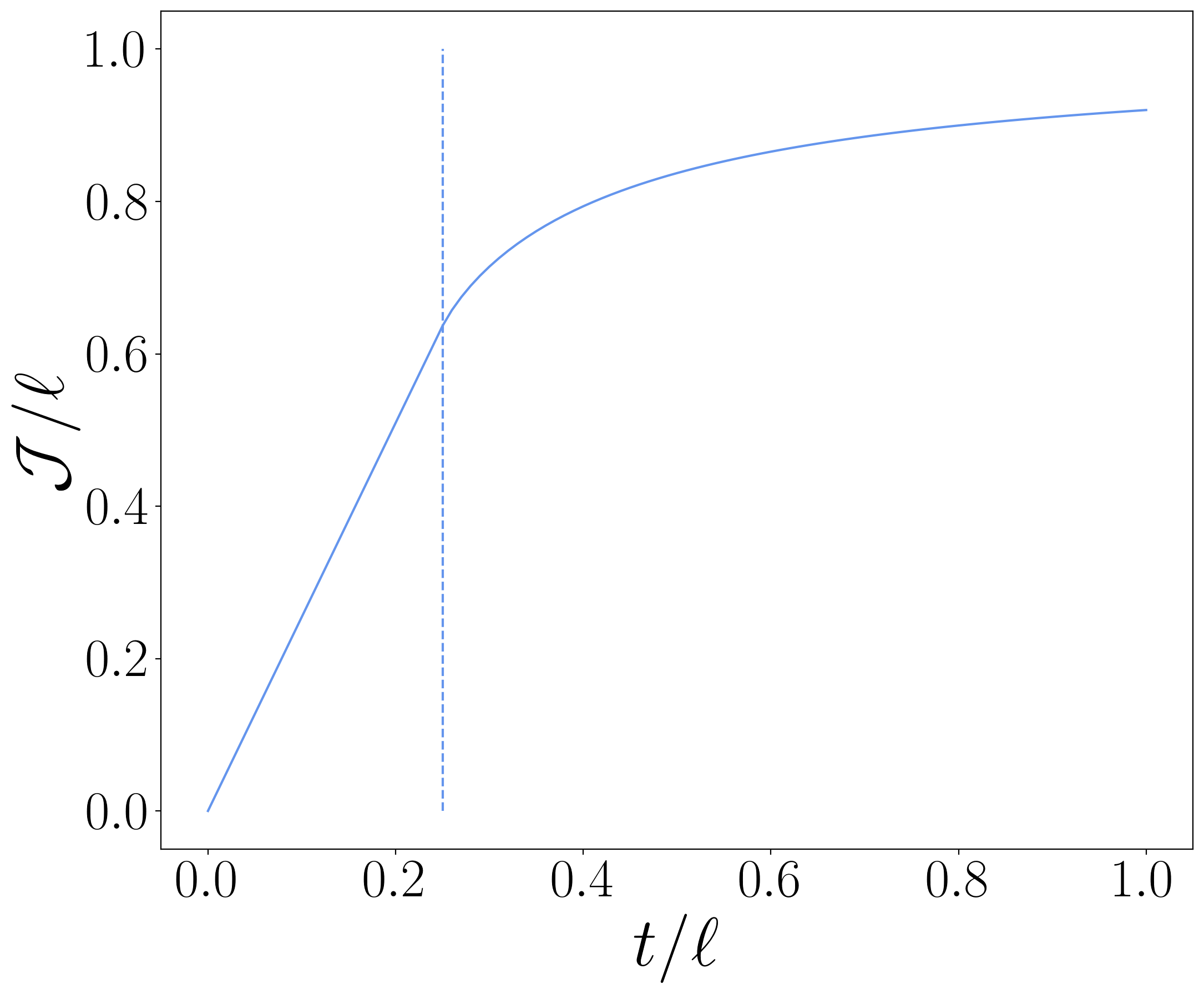
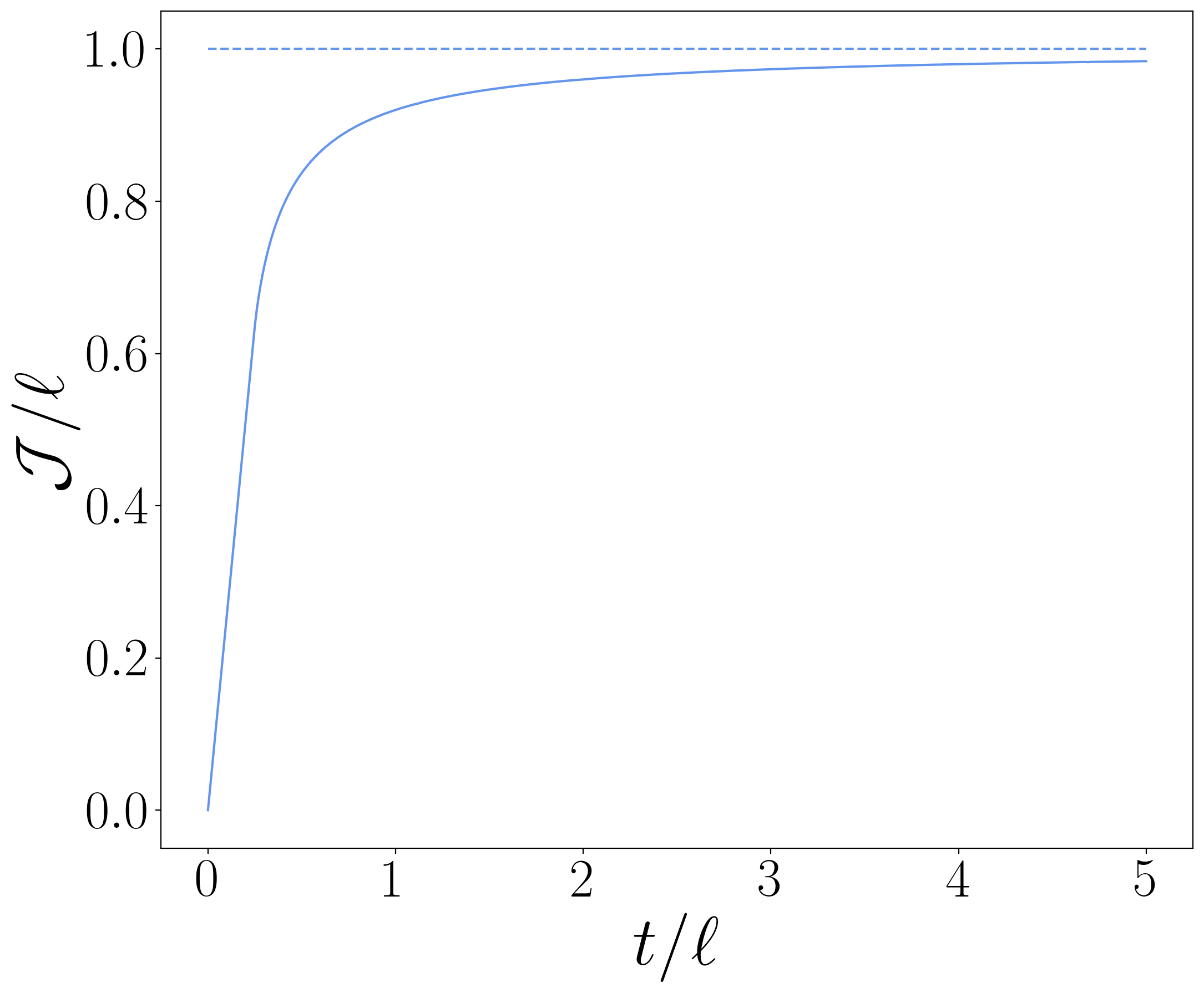
Figure 1: Time evolution of $\mathcal{J}/\ell$ in Eq. (4.8) as a function of $t/\ell$. Left: The crossover between the linear growth and the saturation; the vertical dashed line indicates the time at which the transition occurs, i.e. $t/\ell=1/4$ (in agreement with $t/\ell=1/(2v_{M})$ and $v_{M}=2$). Right: For large time, $\mathcal{J}/\ell$ saturates to $1$ (horizontal dashed line).

The first step to compute the charged moments $Z_{n}(\alpha)$ is the evaluation of the trace of powers of $J_{A}$. With the exact expression (4.2), it is possible to perform this calculation analytically using the multidimentional stationary phase approximation in the scaling limit where $t,\ell~{}\to~{}\infty$ with a fixed finite ratio $t/\ell$. Actually, the computation of $\text{Tr}J_{A}(t)^{j}$ is a simple adaptation of the calculations reported in Ref. [87], and the final result can be written as

$$\text{Tr}J_{A}(t)^{2j}=\ell-\int_{-\pi}^{\pi}\frac{\mathrm{d}k}{2\pi}\min(\ell,2v_{k}t),\quad\text{Tr}J_{A}(t)^{2j+1}=0,$$ (4.3)

with $v_{k}=2|\sin k|$. We note that, with our normalisation, the maximal velocity $v_{M}=\textrm{max}_{k}v_{k}$ is $v_{M}=2$. To compute the charged moments $Z_{n}(\alpha)$, we evaluate the sum (3.7) with (4.3). We use the fact that $\text{Tr}J_{A}(t)^{m}$ only depends on the parity of the exponent for $m>0$, and $\text{Tr}J_{A}(t)^{0}=\ell$. We then find

$$\log Z_{n}(\alpha)=\ell c_{n,\alpha}(0)+\text{Tr}J_{A}(t)^{2}\sum_{m=1}^{\infty}c_{n,\alpha}(2m),$$ (4.4)

where the coefficients $c_{n,\alpha}(k)$ are defined in (3.6). To proceed, we notice that the coefficient $c_{n,\alpha}(0)$, as well as the sum $\sum_{m=1}^{\infty}c_{n,\alpha}(2m)$ in fact correspond to the function $h_{n,\alpha}(x)$ from Eq. (3.6) evaluated in certain simple points. Indeed, we have

$$\begin{split}c_{n,\alpha}(0)&=h_{n,\alpha}(0)=(1-n)\log 2+\log\cos\frac{\alpha}{2}+\mathrm{i}\frac{\alpha}{2},\\ \sum_{m=1}^{\infty}c_{n,\alpha}(2m)&=\left(\frac{h_{n,\alpha}(1)+h_{n,\alpha}(-1)}{2}-c_{n,\alpha}(0)\right)=(n-1)\log 2-\log\cos\frac{\alpha}{2}.\end{split}$$ (4.5)

It immediately follows that

$$\log Z_{n}(\alpha)=\mathrm{i}\ell\frac{\alpha}{2}+\int_{-\pi}^{\pi}\frac{\mathrm{d}k}{2\pi}\mathrm{Re}[h_{n,\alpha}(0)]\min(\ell,2v_{k}t),\quad$$ (4.6)

or

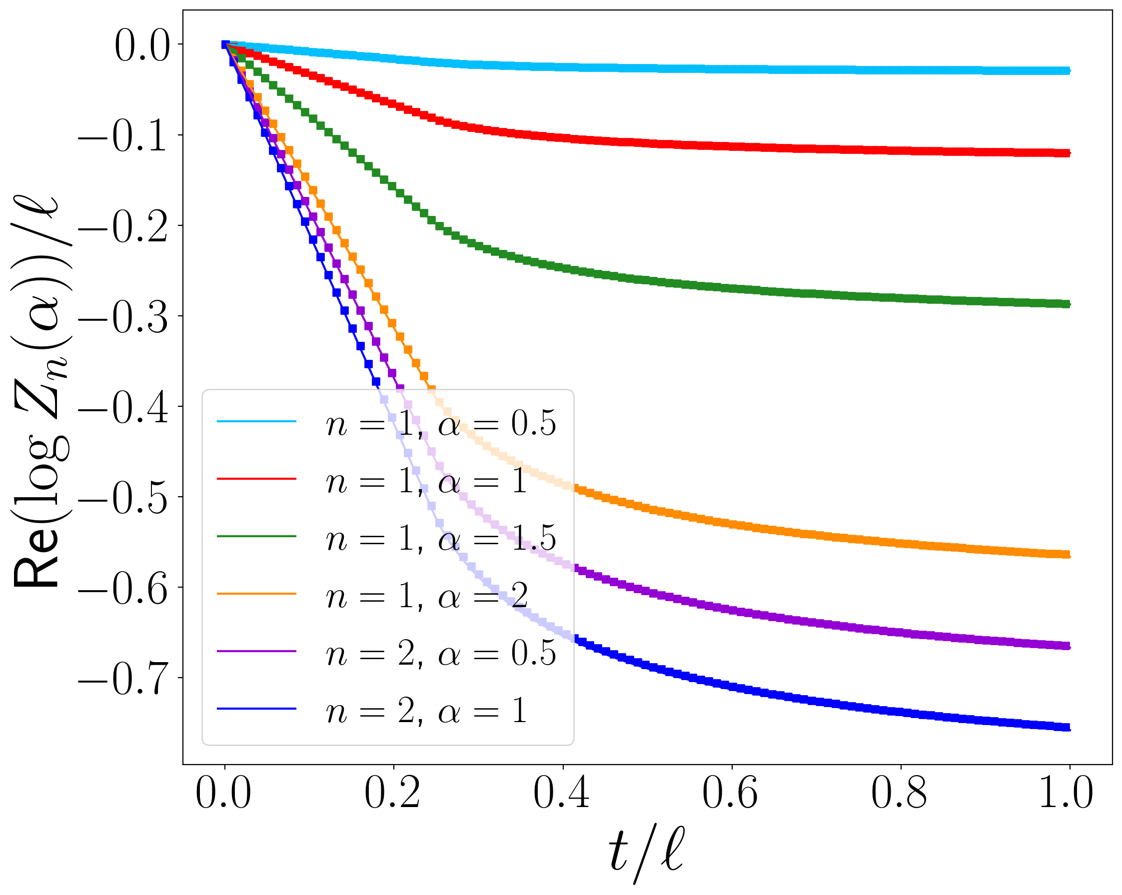
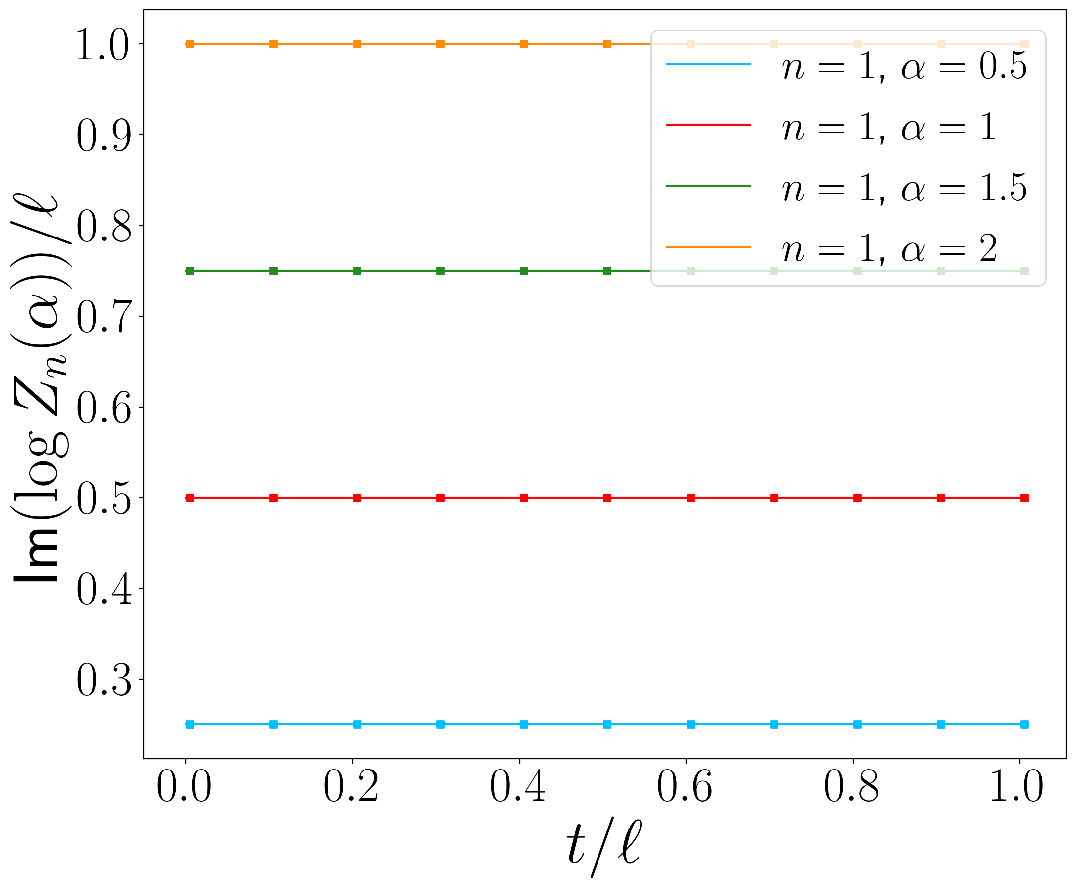
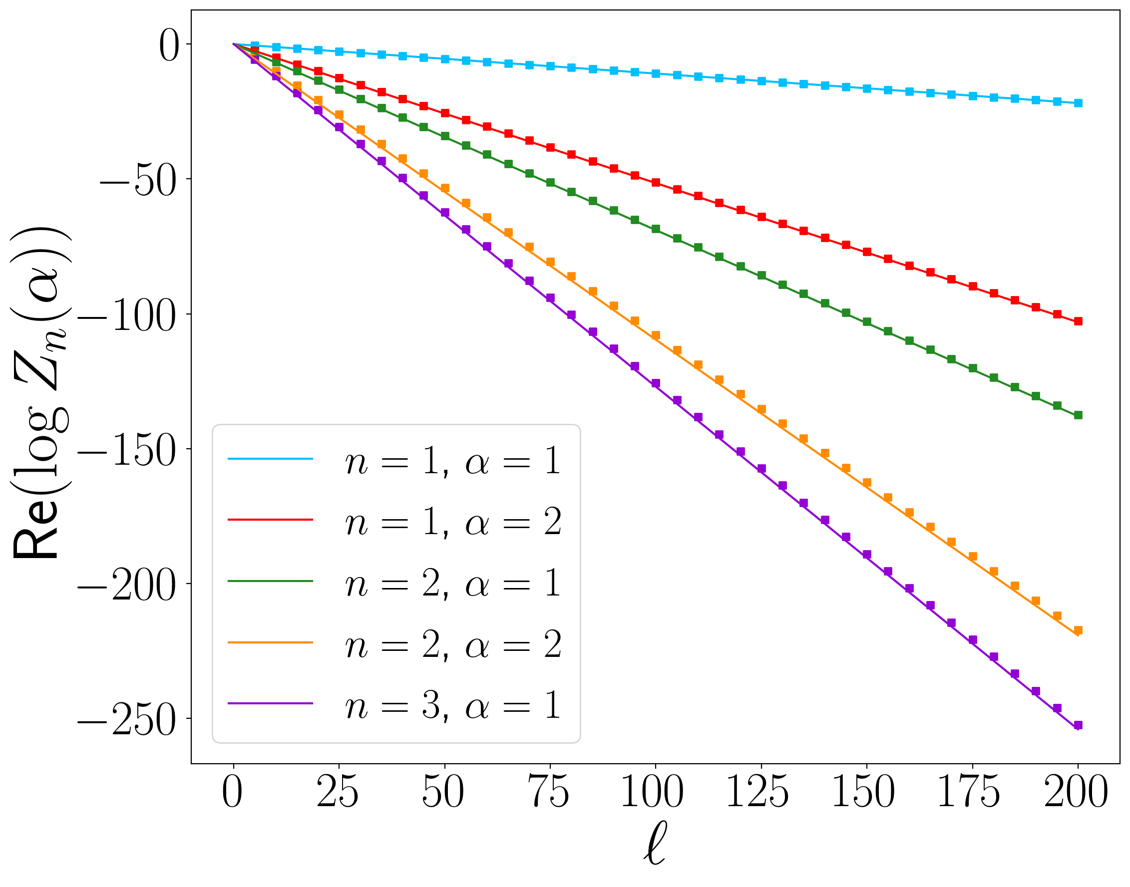
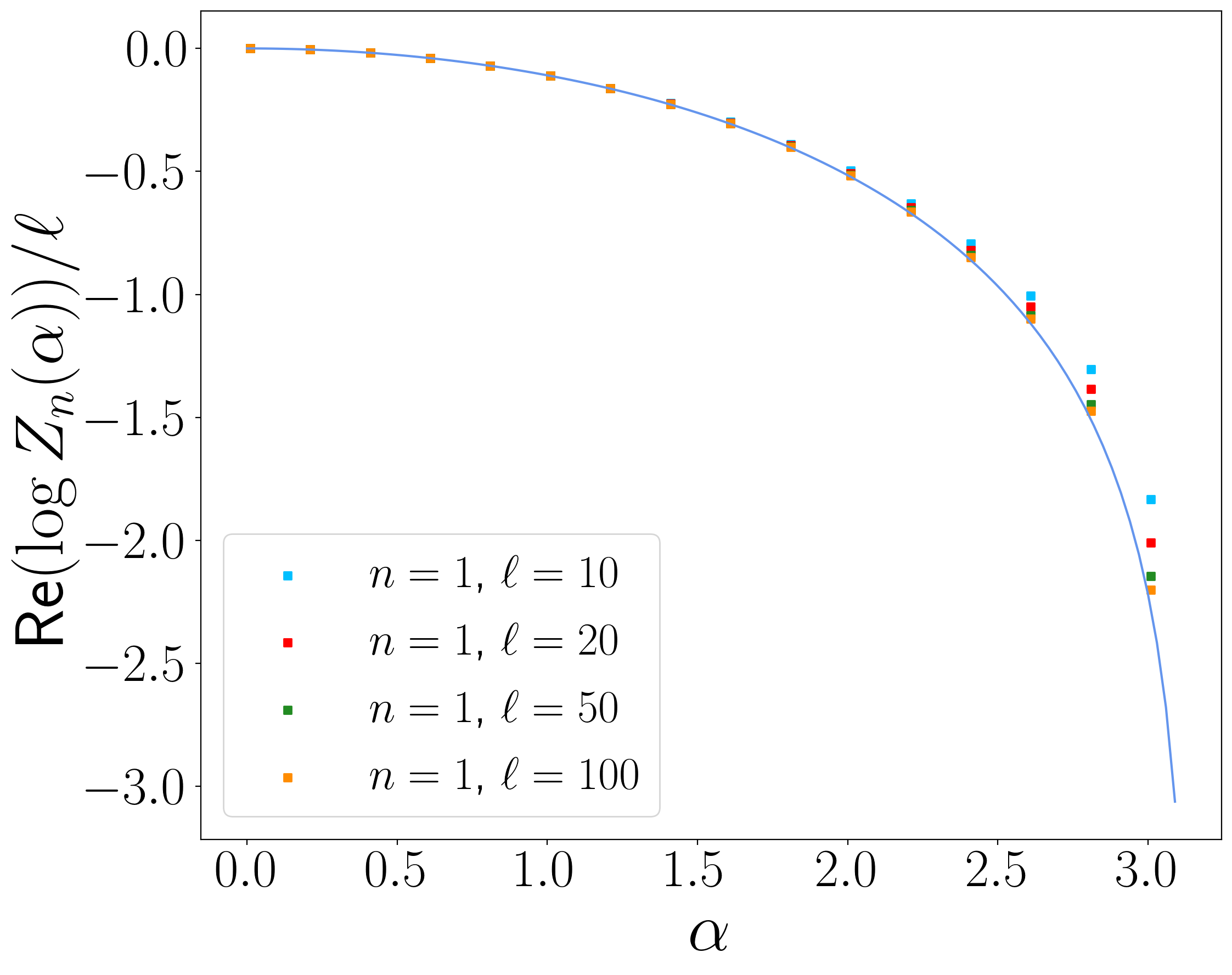
Figure 2: Comparison between the asymptotic result (4.7) (solid lines) and exact numerical data (symbols) for $\log Z_{n}(\alpha)$ after a quench from the Néel state in the free fermion model (3.1). Top left: Time evolution of the real part of $\log Z_{n}(\alpha)$ as a function of $t/\ell$ with $\ell=120$. Top right: Time evolution of the imaginary part of $\log Z_{n}(\alpha)$ as a function of $t/\ell$ with $\ell=20$ and $n=1$. Bottom left: Real part of $\log Z_{n}(\alpha)$ as a function of $\ell$ with $t/\ell=0.5$. Bottom right: Real part of $\log Z_{n}(\alpha)$ as a function of $\alpha$ with $t/\ell=0.5$ and $n=1$.

$$Z_{n}(\alpha)=\left(\frac{\cos\frac{\alpha}{2}}{2^{n-1}}\right)^{\mathcal{J}}\mathsf{e}^{\mathrm{i}\ell\frac{\alpha}{2}}$$ (4.7)

where we introduced the quantity

$$\mathcal{J}\equiv\ell-\text{Tr}J_{A}(t)^{2}=\int_{-\pi}^{\pi}\frac{\mathrm{d}k}{2\pi}\min(\ell,2v_{k}t).$$ (4.8)

The function $\mathcal{J}(t)$ is an increasing function of time, going from $\mathcal{J}(t=0)=0$ to $\mathcal{J}(t=\infty)=\ell$. Its time evolution is separated in two distinct regimes. For short times $t<\ell/(2v_{M})$, $\mathcal{J}(t)\propto t$ increases linearly with time. On the other hand, for $t>\ell/(2v_{M})$, $\mathcal{J}(t)$ slowly saturates to its asymptotic value $\ell$. These behaviours are illustrated in Fig. 1. The ratio $\mathcal{J}(t)/\ell$ is a scaling function of $t/\ell$, a fact that we will use repeatedly in what follows.

In Fig. 2 we compare the prediction (4.7) for the charged moments $Z_{n}(\alpha)$ with ab-initio computations. The dependence of $Z_{n}(\alpha)$ in $t$ and $\ell$ is perfectly reproduced by the exact result, as can be seen from top left, right and bottom left panels. For this quench, the imaginary part is trivial since it is given by the average conserved charge. Concerning the $\alpha$-dependence, we observe that away from $\alpha=\pi$, the analytic prediction and numerical data match perfectly, even for relatively small $\ell$. However, as $\alpha$ gets closer to $\pm\pi$, the difference between the numerical results and the exact prediction gets larger. To highlight this phenomenon, we zoom on the region in the vicinity of $\alpha=\pi$ in Fig. 3. It is clear that for large $\ell$, the data approach the asymptotic result for any $\alpha\neq\pi$. As is well known also in equilibrium, see e.g. [42, 44], as $\alpha$ gets closer to $\pm\pi$, the match between the numerical data and the analytical predictions only holds for very large values of $\ell$. Additional subleading terms (vanishing in the scaling limit) in the expansion of $\mathcal{J}$ should be considered to correctly describe the large corrections in finite size. However, this point will not affect the asymptotic behaviour of the symmetry resolved quantities which are calculated by a saddle point integral close to $\alpha=0$ and will not be further discussed.

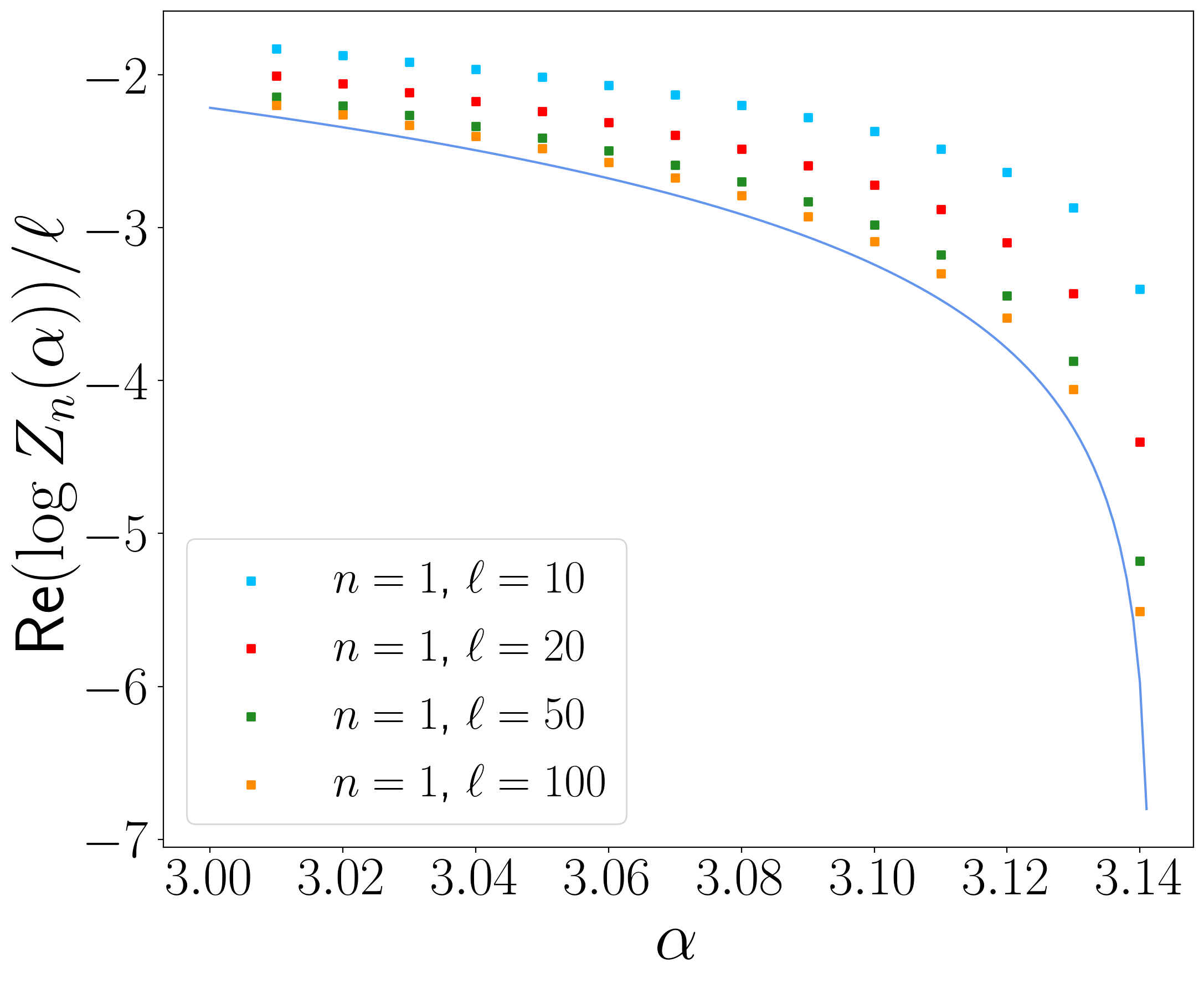
Figure 3: Real part of $\log Z_{n}(\alpha)$ after a quench from the Néel state in the free fermion model (3.1) as a function of $\alpha$ with $t/\ell=0.5$ and $n=1$ near the value $\alpha=\pi$.

4.1.2 Fourier transform

The symmetry resolved moments $\mathcal{Z}_{n}(q)$ with $q=\Delta q+\langle Q_{A}\rangle$ are defined as the Fourier transform of the charged moments $Z_{n}(\alpha)$. Using Eq. (2.6), the asymptotic formula (4.7), and $\langle Q_{A}\rangle=\ell/2$, we have

$$\mathcal{Z}_{n}(q)\simeq 2^{(1-n)\mathcal{J}}\int_{-\pi}^{\pi}\frac{\mathrm{d}\alpha}{2\pi}\left(\cos\frac{\alpha}{2}\right)^{\mathcal{J}}\mathsf{e}^{-\mathrm{i}\alpha\Delta q}.$$ (4.9)

First of all, we stress that this formula is valid for arbitrary $\Delta q$, but only for asymptotically large $\mathcal{J}$ because we used the asymptotic behaviour of $Z_{n}(\alpha)$. Indeed, as we shall see, the integral in Eq. (4.9) can be also negative for small $\mathcal{J}$. Furthermore, in the scaling limit $\Delta q$ should be taken proportional to $\ell$ (or, equivalently, $t$), otherwise one obtains trivial results.

Since the $n$-dependence in Eq. (4.9) is trivial, we focus on $n=1$. The integral in Eq. (4.9) can be evaluated in closed form in terms of the Euler Beta function $B(x,y)=\frac{\Gamma(x)\Gamma(y)}{\Gamma(x+y)}$, where $\Gamma(z)$ is the Gamma function. The result reads [88]

$$\zeta_{1}(q)=2^{-\mathcal{J}}\frac{\Gamma(\mathcal{J}+1)}{\Gamma\big{(}\frac{\mathcal{J}+2\Delta q+2}{2}\big{)}\Gamma\big{(}\frac{\mathcal{J}-2\Delta q+2}{2}\big{)}},$$ (4.10)

and we recall

$${\cal Z}_{1}(q)\simeq\zeta_{1}(q),\qquad\rm{for}\;\mathcal{J}\gg 1.$$ (4.11)

We now discuss the properties of the function $\zeta_{1}(q)$ and in particular its limit for $\mathcal{J}\gg 1$ when it tends to the physical probability ${\cal Z}_{1}(q)$. The function $\Gamma(z)$ has poles when $z$ is a negative integer. Since $\mathcal{J}\geq 0$, it follows that $\zeta_{1}(q)$ vanishes when $\mathcal{J}<2|\Delta q|$ is an even integer. For other values of $\mathcal{J}$ in the regime $\mathcal{J}<2|\Delta q|$, the function $\zeta_{1}(q)$ oscillates in $\ell$ around zero, as can be seen in Fig. 4 (top panels). The amplitude of these oscillations decays quickly to zero and, in the scaling limit, averages to $\zeta_{1}(q)\simeq\mathcal{Z}_{1}(q)\simeq 0$ for all the relevant physics. Actually, the last zero of $\zeta_{1}(q)$ is at position $\mathcal{J}=2|\Delta q|-2$ and afterward it monotonically increases with $\mathcal{J}$ (see Fig. 4, bottom panels). At $\mathcal{J}=2|\Delta q|$, we have $\zeta_{1}(q)=2^{-\mathcal{J}}=2^{-2|\Delta q|}$. Thus, in the scaling limit, when $\Delta q$ also grows with $\ell$, the entire window $2|\Delta q|-2<\mathcal{J}<2|\Delta q|$ shrinks to zero length, and $\mathcal{Z}_{1}(q)$ can be considered zero up to $\mathcal{J}=2|\Delta q|$. Anyhow, for finite $q$, ${\cal Z}_{1}(q)$ is expected to grow from $\mathcal{J}=2|\Delta q|-2$. We illustrate these behaviours in Fig. 4 for relatively small values of $\ell$.

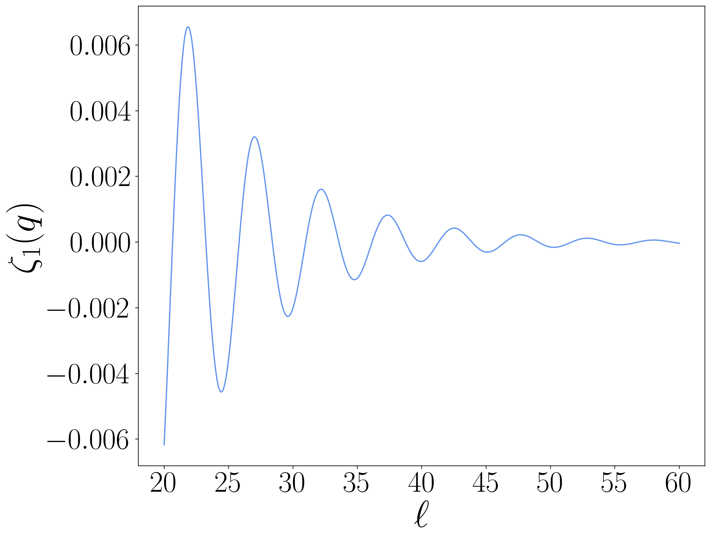
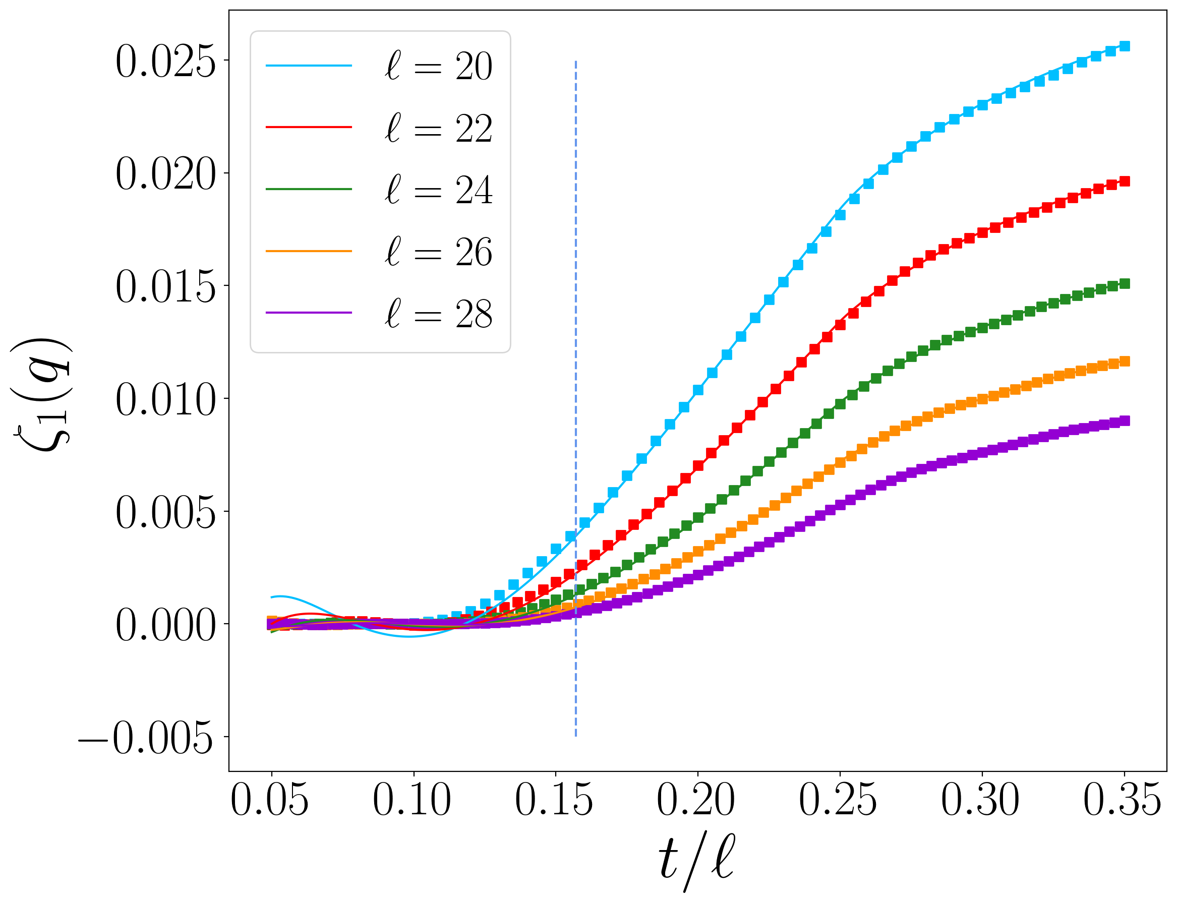
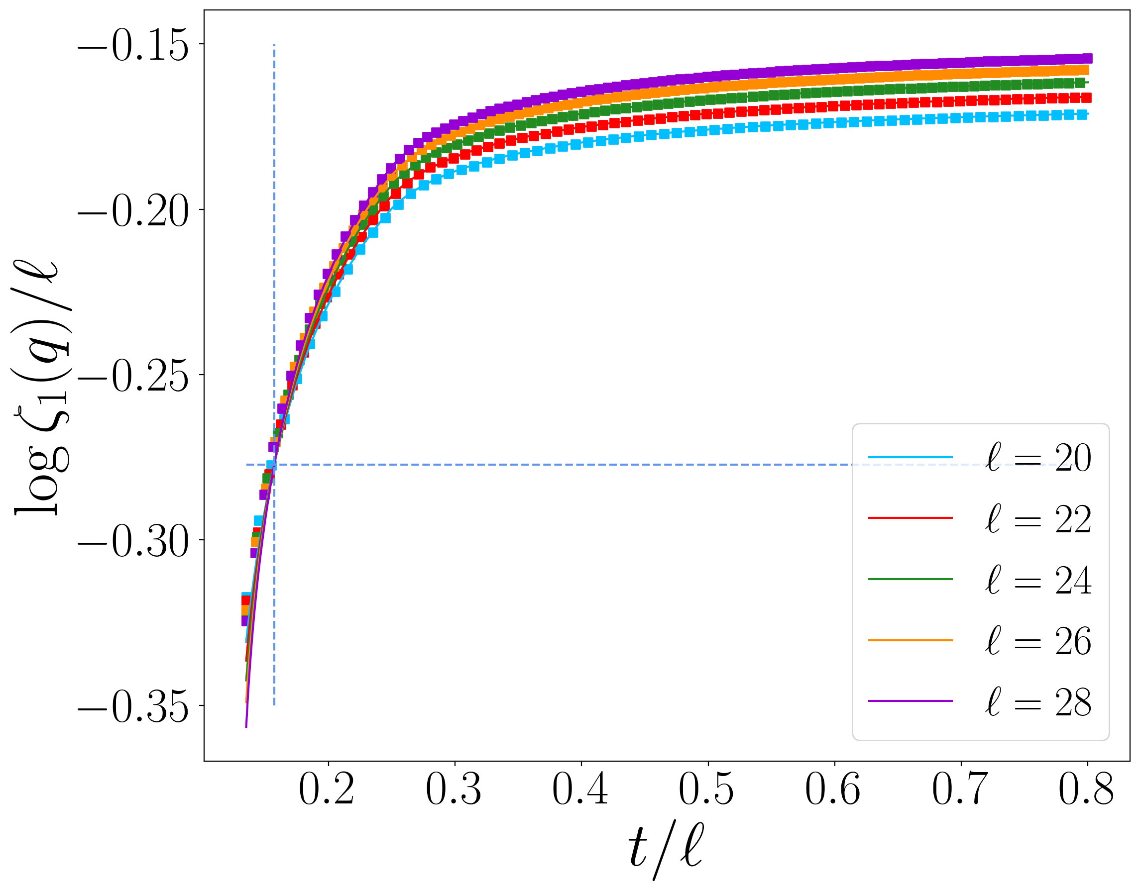
Figure 4: Study of the function $\zeta_{1}(q)$ in Eq. (4.10) that tends to the physical probability $\mathcal{Z}_{1}(q)$ for large $\mathcal{J}$ after a quench from the Néel state in the tight-biding model (3.1). Top: Short time regime $\mathcal{J}<2|\Delta q|$. Left: $\zeta_{1}(q)$ as a function of $\mathcal{J}/\ell$ for $q=\ell$ and various values of $\ell$. As $\ell$ increases, $\zeta_{1}(q)$ quickly averages to zero. Right: $\zeta_{1}(q)$ as a function of $\ell$ with $q=9\ell/10$ and fixed $\mathcal{J}=\ell/100$. Bottom: $\zeta_{1}(q)$ (left) and $(\log\zeta_{1}(q))/\ell$ (right) as a function of $\mathcal{J}/\ell$ with $q=7\ell/10$. We compare the exact formula of Eq. (4.10) for $\zeta_{1}(q)$ (solid lines) with numerical data for $\mathcal{Z}_{1}(q)$ (symbols). The vertical dashed lines are placed at $\mathcal{J}/\ell=2|\Delta q|/\ell=2/5$ in both panels. Left: $\zeta_{1}(q)$ starts growing monotonically at $\mathcal{J}=2|\Delta q|-2$. Right: The horizontal dashed line is at position $\log\zeta_{1}(q)=-2|\Delta q|\log 2$. All the curves collapse on the point $\zeta_{1}(q)=2^{-\mathcal{J}}$ at $\mathcal{J}=2|\Delta q|$.

In the regime $\mathcal{J}>2|\Delta q|\gg 1$, we use Stirling formula to derive the asymptotic behaviour of $\zeta_{1}(q)$ and hence of $\mathcal{Z}_{1}(q)$. We find

$$\log\mathcal{Z}_{1}(q)=-\Big{(}\frac{\mathcal{J}}{2}+|\Delta q|\Big{)}\log\Big{(}1+\frac{2|\Delta q|}{\mathcal{J}}\Big{)}-\Big{(}\frac{\mathcal{J}}{2}-|\Delta q|\Big{)}\log\Big{(}1-\frac{2|\Delta q|}{\mathcal{J}}\Big{)}\\ +\frac{1}{2}\log\Big{(}\frac{4\mathcal{J}}{(\mathcal{J}+2\Delta q)(\mathcal{J}-2\Delta q)}\Big{)}-\frac{1}{2}\log 2\pi.$$ (4.12)

The first line of Eq. (4.12) contains the leading terms, the second one gives the first corrections, and sub-leading terms are omitted. We stress that the corrections due to the subleading terms in $Z_{n}(\alpha)$ enter at an order higher than the ones in Eq. (4.12).

We have seen that in the scaling regime $\mathcal{Z}_{1}(q)$ is zero for short $\mathcal{J}$ and starts growing at $\mathcal{J}=2\Delta q$. These relations can be transferred from the auxiliary variable $\mathcal{J}$ to the physical time $t$. The crossover between the zero probability regime and the growing one takes place at a time $t_{D}$ that we dub delay time. The latter is defined by the relation $\mathcal{J}(t_{D})=2|\Delta q|$. In general, this relation is not explicit. However, from Eq. (4.8), we have that for $2v_{M}t<\ell$

$$\mathcal{J}=2t\int_{-\pi}^{\pi}\frac{\mathrm{d}k}{2\pi}v_{k},\quad 2v_{M}t<\ell.$$ (4.13)

Since $v_{k}=2|\sin k|$ and $v_{M}=2$, we find

$$4t_{D}\int_{-\pi}^{\pi}\frac{\mathrm{d}k}{2\pi}|\sin k|=2|\Delta q|,\quad 4t_{D}<\ell,$$ (4.14)

and conclude

$$t_{D}=\pi\frac{|\Delta q|}{4},\quad{\rm for}\quad|\Delta q|<\frac{\ell}{\pi}.$$ (4.15)

For larger $|\Delta q|$, there is no closed form for $t_{D}$. In Fig. 5 we compare the numerical solution of $\mathcal{J}(t_{D})=2|\Delta q|$ (symbols) with the linear result $t_{D}=\pi\frac{|\Delta q|}{4}$ (solid line). For $|\Delta q|<\frac{\ell}{\pi}$ the match is perfect, but for larger $\Delta q$ the delay grows very quickly.

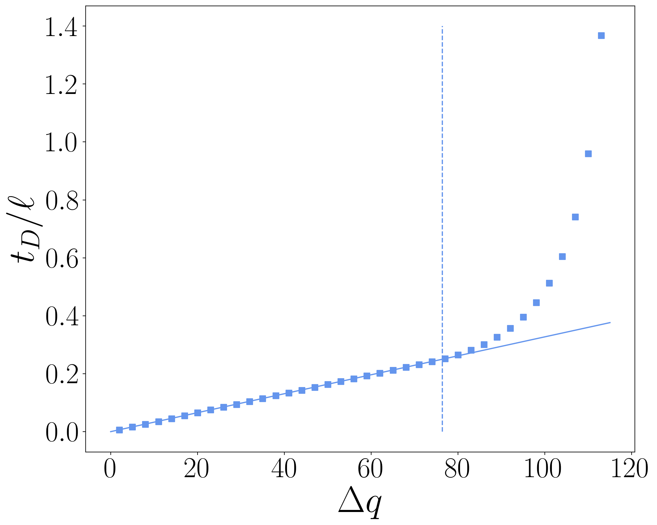
Figure 5: Delay $t_{D}$ obtained from the numerical solution of $\mathcal{J}(t_{D})=2|\Delta q|$ for $\ell=240$ (symbols) compared with the linear result $t_{D}=\pi\frac{|\Delta q|}{4}$ (solid line), valid up to $\Delta q=\frac{\ell}{\pi}$ (dashed vertical line).

Even though the scaling behaviour of $\mathcal{Z}_{1}(q)$ is completely encoded in Eq. (4.10), we also analyse it with the saddle point approximation. The reason is that this method is useful in the cases where there are no analytical formulas like Eq. (4.10). We recast Eq. (4.9) as

$$\mathcal{Z}_{1}(q)=\int_{-\pi}^{\pi}\frac{\mathrm{d}\alpha}{2\pi}\mathsf{e}^{\ell h(\alpha)},\quad h(\alpha)=-\mathrm{i}\alpha\frac{\Delta q}{\ell}+\frac{\mathcal{J}}{\ell}\log\cos\frac{\alpha}{2},$$ (4.16)

so that the saddle point $\alpha^{*}$, defined as $h^{\prime}(\alpha^{*})=0$, is

$$\alpha^{*}=-2\mathrm{i}\,{\rm arctanh}\left(\frac{2\Delta q}{\mathcal{J}}\right)\\ =\mathrm{i}\log\left(\frac{\mathcal{J}-2\Delta q}{\mathcal{J}+2\Delta q}\right).$$ (4.17)

We have two regimes, (i) $\mathcal{J}<2|\Delta q|$, where $\alpha^{*}$ has a real part, and (ii) $\mathcal{J}>2|\Delta q|$, where $\alpha^{*}$ is purely imaginary. In the first regime, the real part of $\alpha^{*}$ leads to a non-zero imaginary part of $h(\alpha^{*})$ and $\mathcal{Z}_{1}(q)$ oscillates quickly in $\ell$ around zero. This behaviour is the same as the one we found by analyzing the exact formula (4.10). In the scaling limit, these oscillations average to zero for all the relevant physics.

Conversely, for $t>t_{D}$ (i.e. $\mathcal{J}>2|\Delta q|$), we deform the integration contour to pass through $\alpha^{*}$ while remaining in the analyticity region of the integrand. The saddle point method gives

$$\mathcal{Z}_{1}(q)=\mathsf{e}^{\ell h(\alpha^{*})}\sqrt{\frac{1}{2\pi\ell|h^{\prime\prime}(\alpha^{*})|}}.$$ (4.18)

The logarithm of this equation precisely gives back Eq. (4.12), as expected. In the limit where $\mathcal{J}\gg|\Delta q|$ we have

$$\mathcal{Z}_{1}(q)\simeq\sqrt{\frac{2}{\mathcal{J}\pi}}\mathsf{e}^{-\frac{2\Delta q^{2}}{\mathcal{J}}}$$ (4.19)

at leading order.

4.1.3 Symmetry resolved Rényi entropies

We now turn to the evaluation of the symmetry resolved Rényi entropies. Plugging Eq. (4.9) into Eq. (2.7), $S_{n}(q)$ reads

$$\begin{split}S_{n}(q)&=\mathcal{J}\log 2+\log\mathcal{Z}_{1}(q)\\ \end{split}$$ (4.20)

and does not depend on $n$. In the scaling regime $\mathcal{J}>2|\Delta q|\gg 1$, $\log\mathcal{Z}_{1}(q)$ is given by (4.12).

Following the discussion of the previous section, in the scaling limit, the entropies start to grow for $t>t_{D}$. In the top panels of Fig. 6, we compare ab-initio calculations of $S_{n}(q)$ and the exact prediction (4.20), finding perfect agreement. In particular, Fig. 6 convincingly shows that the numerical results for $S_{n}(q)$ do not depend on $n$. We thus focus on $S_{1}(q)$ for the rest of this subsection. We also compare the prediction (4.15) for the delay with the numerical results at a finite $\ell$ (we fix $\ell=240$ and we calculated the delay time as the time when $S_{1}(q)/\ell=0.007$) in the bottom right panel of Fig. 6 and again find a very good agreement.

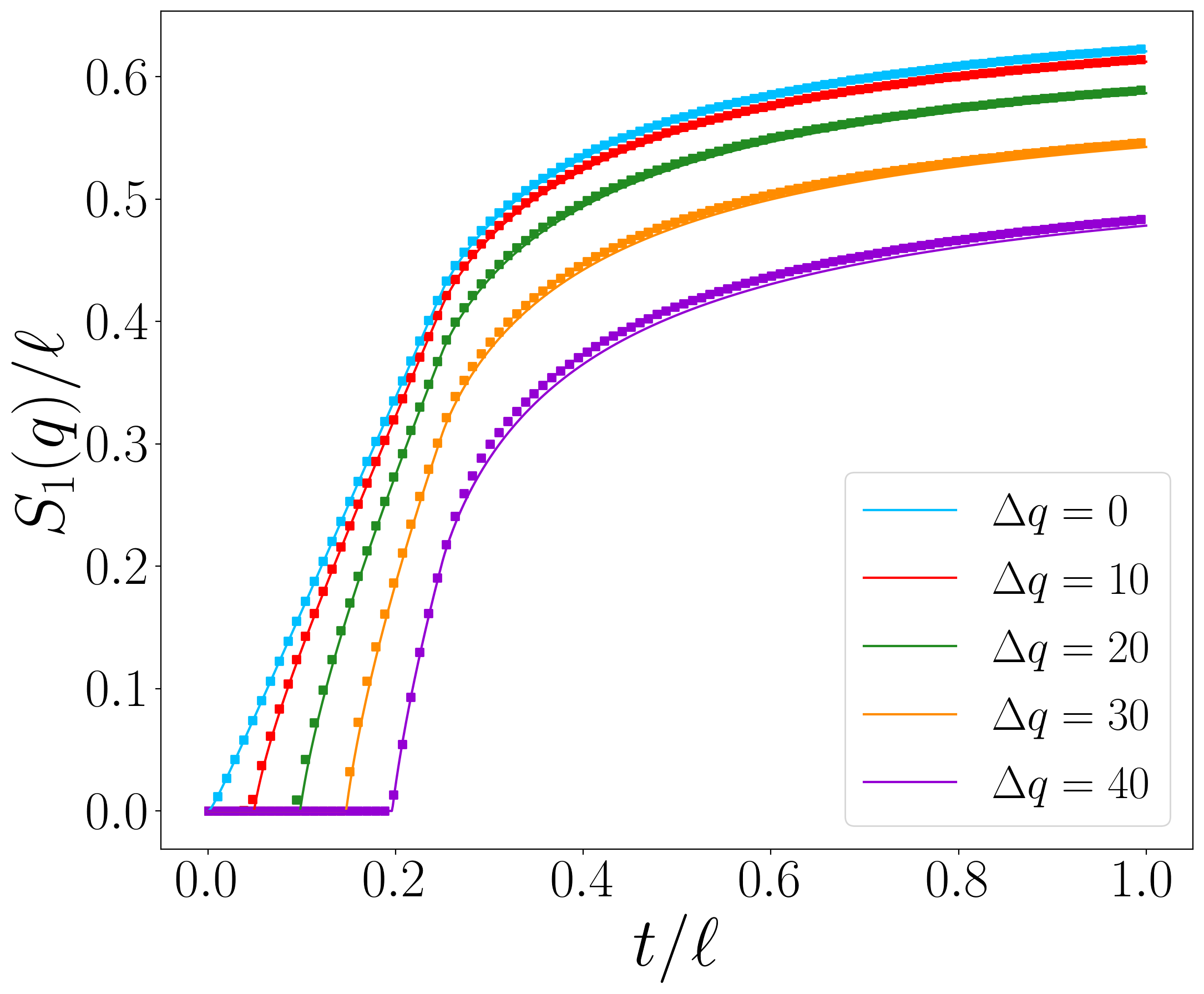
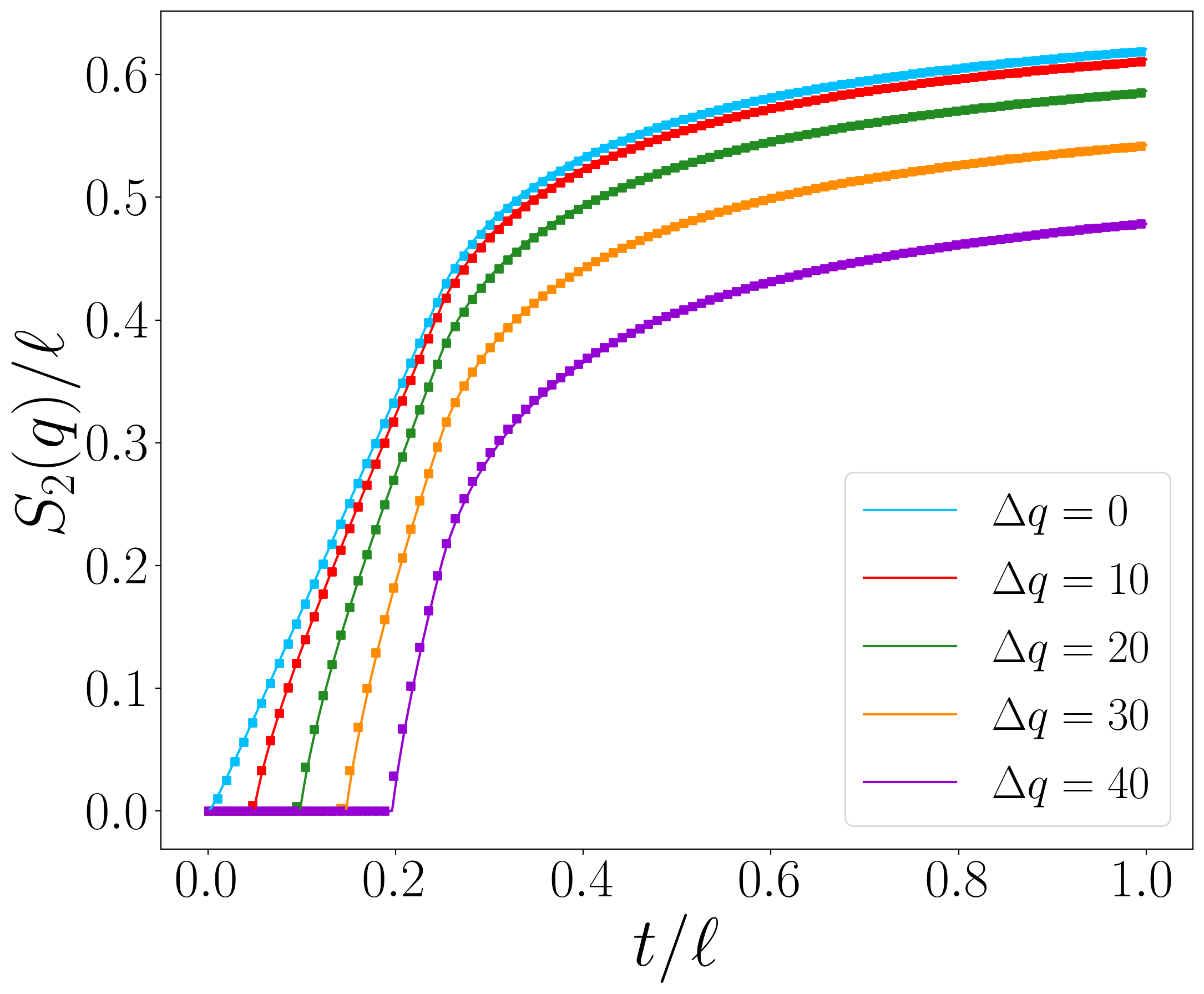
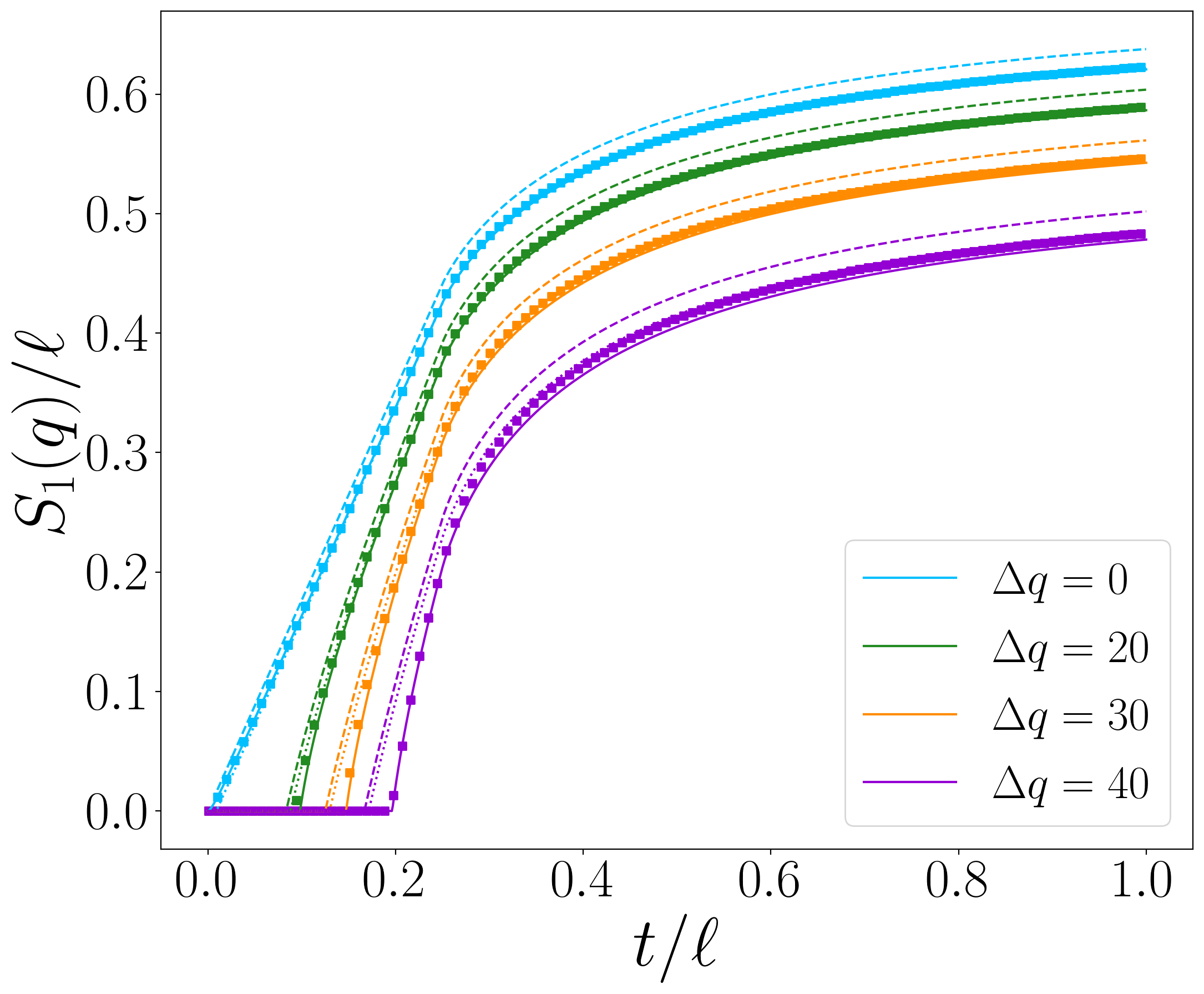
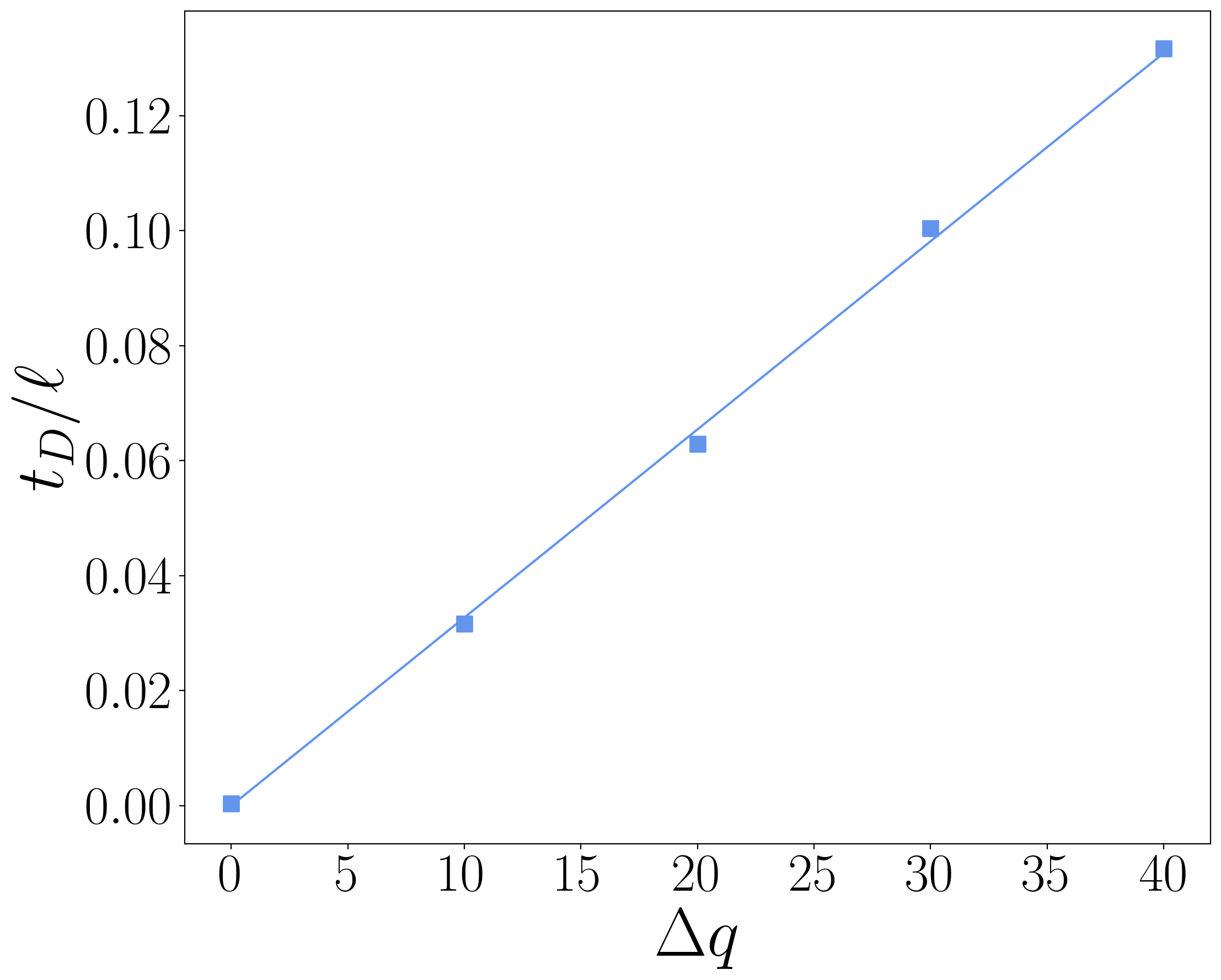
Figure 6: Top and bottom left: Time evolution of the symmetry resolved entanglement entropies $S_{n}(q)$ after a quench from the Néel state in the tight-binding model (3.1). The symbols are the exact numerical results for $\ell=160$ and various $\Delta q$. The solid lines are our prediction (4.20) that perfectly match the numerical data. Bottom left: The dashed lines are the saddle-point approximation (4.21) and the dotted ones are the same approximation with the logarithmic correction. Bottom right: Delay time $t_{D}$ for various $\Delta q$ and $\ell=240.$ The solid line is the analytic prediction (4.15) and the symbols are the numerical results. They are obtained as the time for which $S_{1}(q)/\ell=0.007$.

If in the scaling limit with $\ell$, we also take $\mathcal{J}\gg|\Delta q|$, we can use Eq. (4.12) and plug it into (4.20). Expanding the result in powers of $|\Delta q|/\mathcal{J}$, we find

$$S_{n}(q)=\mathcal{J}\left(\log 2-2\Big{(}\frac{\Delta q}{\mathcal{J}}\Big{)}^{2}\right).$$ (4.21)

Eq. (4.21) implies that for small $|\Delta q|$ there is an effective equipartition of entanglement between the various symmetry sectors, with violations of order $(\Delta q)^{2}/\ell$. We report this prediction as dashed lines in the bottom left panel of Fig. 6. There appears to be some discrepancies, close to the delay time, between this approximation and the numerical results, even for small $|\Delta q|$, where one would expect the approximation to be very accurate. The reason for such disagreement is, obviously, that at the delay time $\mathcal{J}(t_{D})=0$ and so the subleading terms in (4.21) cannot be neglected. Looking at Eq. (4.12) (or equivalently Eq. (4.18)), we see that the first correction to $S_{n}(q)$ in the large-$\ell$ expansion is proportional to $\log\ell$. In the same panel of Fig. 6, we add this correction and report $\frac{\mathcal{J}}{\ell}\left(\log 2-2\Big{(}\frac{\Delta q}{\mathcal{J}}\Big{)}^{2}\right)-1/(2\ell)\log\ell$ as the dotted lines. These curves get closer to the numerical data and fit them perfectly for $t\gg t_{D}$, i,e, in the region where $\mathcal{J}$ is significantly larger than $|\Delta q|$. This correction is subleading in the scaling limit and hence we conclude that Eq. (4.21) correctly reproduces the numerical data in the large-$\ell$ limit.

4.1.4 Total and number entropy

A final question worth investigating is whether our results for the symmetry resolved entanglement entropy are coherent with the known results for the dynamics of the total entanglement entropy $S_{1}$. To this aim, we should also investigate the contribution of the number entropy $S^{n}$ to the total entanglement. The number entropy $S^{n}$ is defined in Eq. (2.2), providing in our case

$$S^{n}=-\sum\limits_{q=0}^{\ell}\mathcal{Z}_{1}(q)\log\mathcal{Z}_{1}(q)$$ (4.22)

and, using the same asymptotic calculations as in Sec. 4.1.2 and Eq. (4.19), we find

$$S^{n}=\sqrt{\frac{2}{\mathcal{J}\pi}}\sum_{\Delta q=-\ell/2}^{\ell/2}\Big{(}\frac{2\Delta q^{2}}{\mathcal{J}}+\frac{1}{2}\log\frac{\mathcal{J}\pi}{2}\Big{)}\mathsf{e}^{-\frac{2\Delta q^{2}}{\mathcal{J}}}$$ (4.23)

for $\mathcal{J}\gg|\Delta q|$. The latter condition is not met for the extreme values of $|\Delta q|$ in the sum, where instead we have $\mathcal{J}\sim|\Delta q|$. However, such values of the subsystem charge have a very low probability and so this approximation is expected to give excellent results, as we will soon confirm numerically. Since we are in the limit of large $\ell$, we transform the sums into Gaussian integrals. Their evaluation is straightforward and we have

$$S^{n}=\frac{1}{2}\Big{(}1+\log\frac{\mathcal{J}\pi}{2}\Big{)},$$ (4.24)

i.e. the number entropy grows logarithmically with time until saturation to a value which is proportional to $\log\ell$. Such behaviour is reminiscent of what found in many other different contexts [73, 74, 77].

In Fig. 7 we compare this result (solid lines) with ab-initio calculations of $S^{n}$ (symbols), and find perfect agreement. The inset in the left panel shows the time-evolution of $S^{n}$ in a log-linear scale and highlights the logarithmic growth in time before the saturation. It directly follows from Eq. (4.24) that the large-time limit of the number entropy is $\displaystyle\lim_{t\to\infty}S^{n}=\frac{1}{2}\Big{(}1+\log\frac{\ell\pi}{2}\Big{)}$, reported as a dotted horizontal line in the left panel of Fig. 7. This analysis shows that in the scaling limit, the number entropy has a negligible contribution to the total entropy, $\displaystyle\lim_{t\to\infty}S^{n}/S_{1}=\mathcal{O}(\ell^{-1}\log\ell)$.

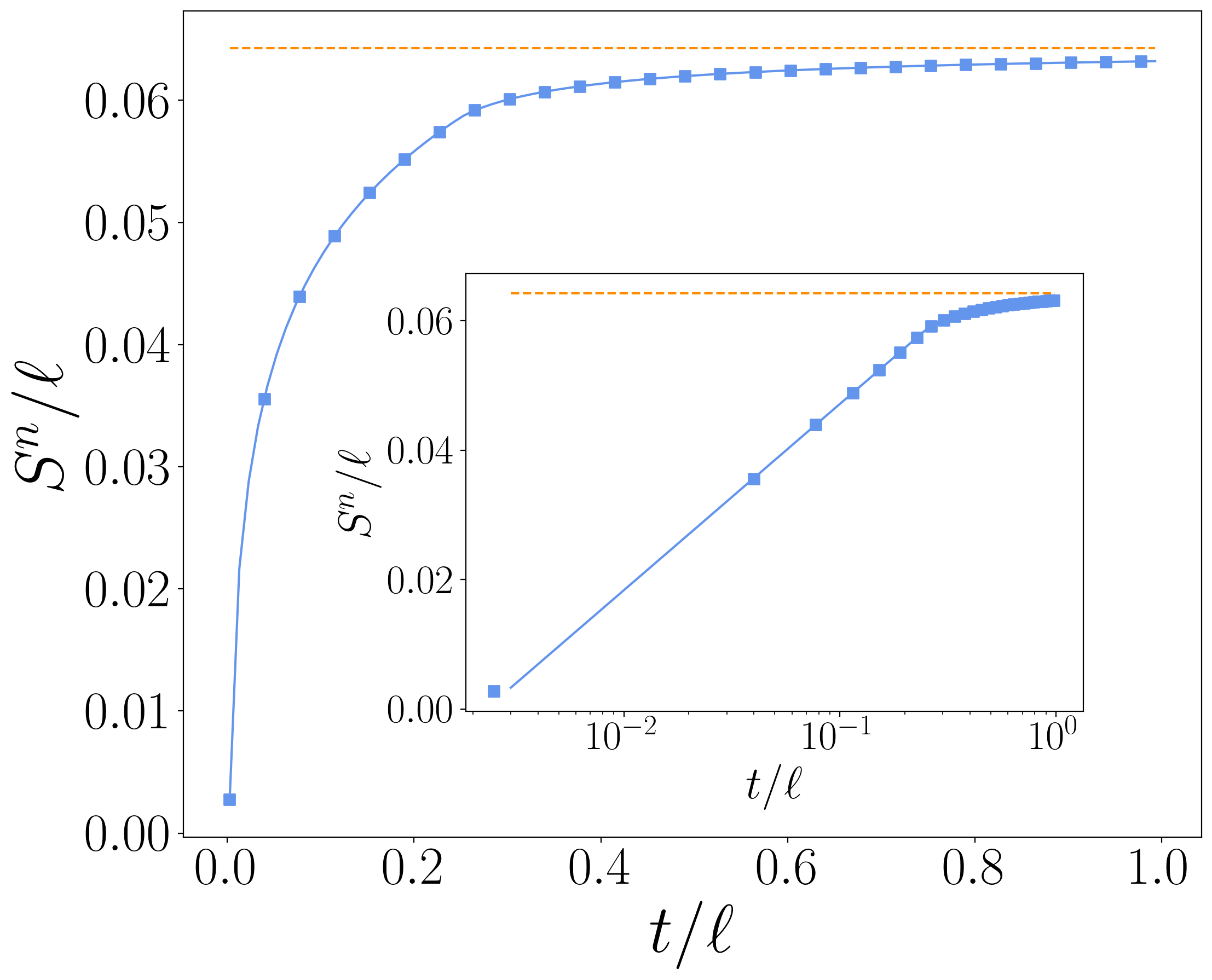
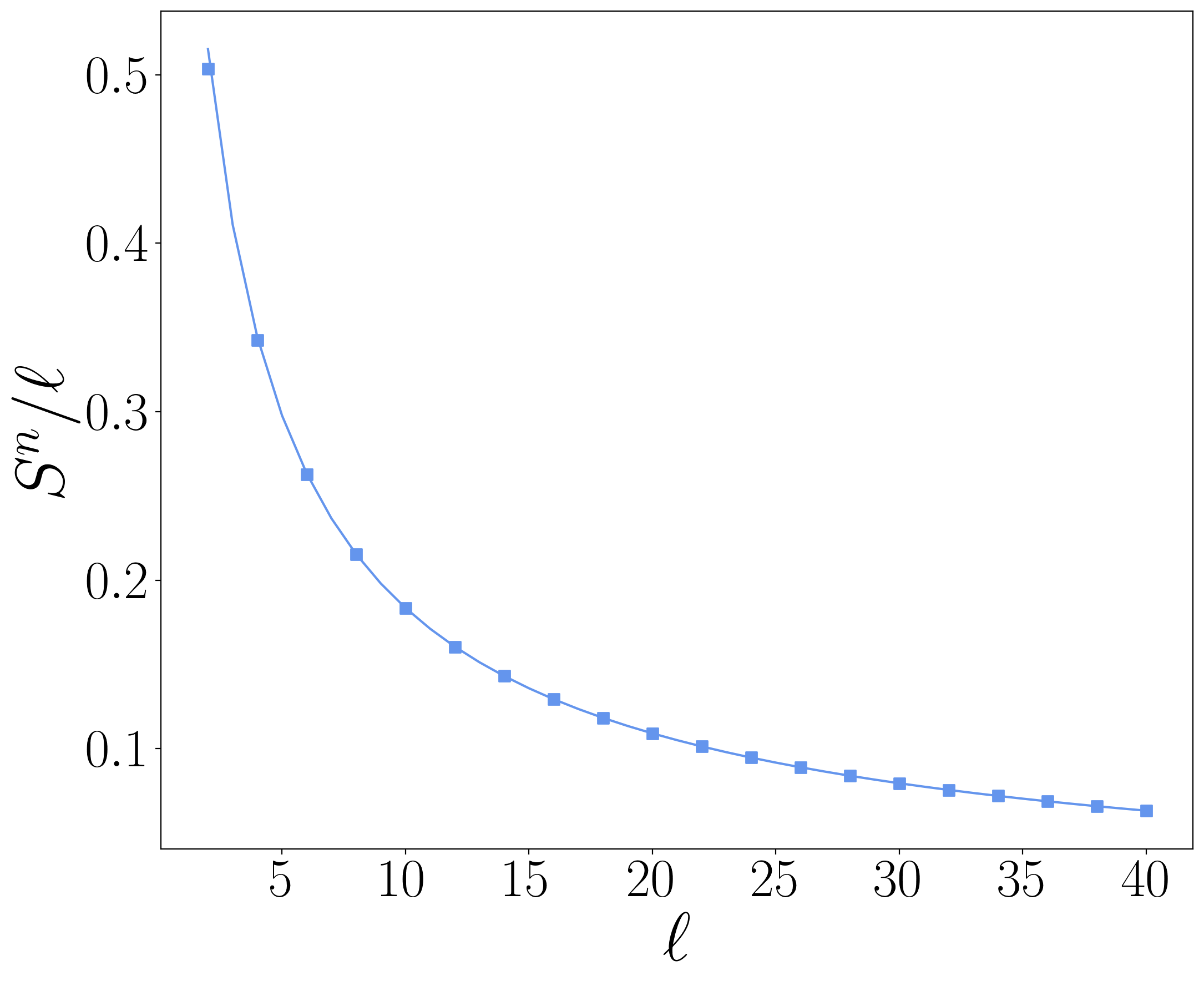
Figure 7: Evolution of $S^{n}$ after a quench from the Néel state in the tight-binding model (3.1) as a function of $t/\ell$ for $\ell=40$ (left panel), and as a function of $\ell$ with $t/\ell=1$ (right panel). The prediction (4.24) (solid line) perfectly matches the numerical results (symbols). In the left panel, the horizontal dotted line is the asymptotic value $\frac{1}{2\ell}\Big{(}1+\log\frac{\ell\pi}{2}\Big{)}$ for large times. In the same panel, the inset shows $S^{n}$ as a function of $t/\ell$ in a log-linear scale.

For the total entropy, we plug Eq. (4.20) into Eq. (2.2) and find

$$S_{1}=\sum_{q=0}^{\ell}\mathcal{Z}_{1}(q)\mathcal{J}\log 2,$$ (4.25)

where we used the relation $p(q)=\mathcal{Z}_{1}(q)$ from Eq. (2.8). The latter satisfies $\sum_{q=0}^{\ell}\mathcal{Z}_{1}(q)=1$, as it should. We thus recover the known result for the total entanglement entropy after a quench from the Néel state [32, 33], namely

$$S_{1}=\log 2\int\frac{\mathrm{d}k}{2\pi}\min(\ell,2v_{k}t).$$ (4.26)

For large times, we have $\displaystyle\lim_{t\to\infty}S_{1}=\ell\log 2$. We finally mention that it is straightforward to show that the number entropy exactly compensate for the $\log\ell$ subleading corrections present in the entanglement of each symmetry sector.

4.2 Disjoint intervals

In this subsection, we move to the analysis of the charged and symmetry resolved entropies for two disjoint intervals, as well as the symmetry resolved mutual information.

The starting point is the correlation matrix $C_{A_{1}\cup A_{2}}(t)$ that encodes correlations within the system $A=A_{1}\cup A_{2}$ where the two subsystems have respective lengths $\ell_{1}$ and $\ell_{2}=\ell-\ell_{1}$, and are separated by $d$ lattice sites. The correlation matrix has the form

$$C_{A_{1}\cup A_{2}}(t)=\begin{pmatrix}C_{11}(t)&C_{12}(t)\\ C_{21}(t)&C_{22}(t)\end{pmatrix}$$ (4.27)

with

$$[C_{11}(t)]_{j,k} =[C(t)]_{j,k},\quad j,k=1,\dots\ell_{1},$$ (4.28)

$$[C_{22}(t)]_{j,k} =[C(t)]_{j+d,k+d},\quad j,k=1,\dots\ell_{2},$$ (4.29)

$$[C_{12}(t)]_{j,k} =[C(t)]_{j,k+d},\quad j=1,\dots\ell_{1},\quad k=1,\dots\ell_{2},$$ (4.30)

$$[C_{21}(t)]_{j,k} =[C(t)]_{j+d,k},\quad j=1,\dots\ell_{2},\quad k=1,\dots\ell_{1},$$ (4.31)

where the matrix elements are given in Eq. (4.1).

4.2.1 Charged moments

In order to compute the charged moments and the symmetry resolved entanglement measures, we compute the trace of arbitrary powers of the matrix $J_{A_{1}\cup A_{2}}(t)=2C_{A_{1}\cup A_{2}}(t)-\mathbb{I}_{\ell}$. We perform the computation of $\text{Tr}J_{A_{1}\cup A_{2}}(t)^{m}$ in the scaling limit $t,\ell,\ell_{1},\ell_{2},d\to\infty$ where the various ratios are kept constant. The calculation uses the multidimensional stationary phase approximation, and generalises the methods used in [87] to the case of an arbitrary separation $d$, see [89]. We find

$$\begin{split}\text{Tr}J_{A_{1}\cup A_{2}}(t)^{2j}&=\ell-\int\frac{\mathrm{d}k}{2\pi}[\min(\ell_{1},2v_{k}t)+\min(\ell_{2},2v_{k}t)]\\ &+\int\frac{\mathrm{d}k}{2\pi}[\max(d,2v_{k}t)+\max(d+\ell,2v_{k}t)-\max(d+\ell_{1},2v_{k}t)-\max(d+\ell_{2},2v_{k}t)],\\ \text{Tr}J_{A_{1}\cup A_{2}}(t)^{2j+1}&=0,\end{split}$$ (4.32)

with $v_{k}=2|\sin k|$. We note that the case $d=0$ reduces to the known result of Eq. (4.3) for a single interval. The computation of the charged moments $Z_{n}^{A_{1}\cup A_{2}}(\alpha)$ proceeds exactly as for the case of a single interval discussed in Sec. 4.1.1. We thus find

$$Z_{n}^{A_{1}\cup A_{2}}(\alpha)=\left(\frac{\cos\frac{\alpha}{2}}{2^{n-1}}\right)^{\mathcal{J}_{d}}\mathsf{e}^{\mathrm{i}\ell\frac{\alpha}{2}}$$ (4.33)

where we introduced

$$\begin{split}\mathcal{J}_{d}\equiv&\ell-\text{Tr}J_{{A_{1}\cup A_{2}}}(t)^{2}\\ =&\int\frac{\mathrm{d}k}{2\pi}[\min(\ell_{1},2v_{k}t)+\min(\ell_{2},2v_{k}t)]\\ &-\int\frac{\mathrm{d}k}{2\pi}[\max(d,2v_{k}t)+\max(d+\ell,2v_{k}t)-\max(d+\ell_{1},2v_{k}t)-\max(d+\ell_{2},2v_{k}t)].\end{split}$$ (4.34)

In Fig. 8 we compare the prediction (4.33) for $Z_{n}^{A_{1}\cup A_{2}}(\alpha)$ with ab-initio calculations and find perfect agreement.

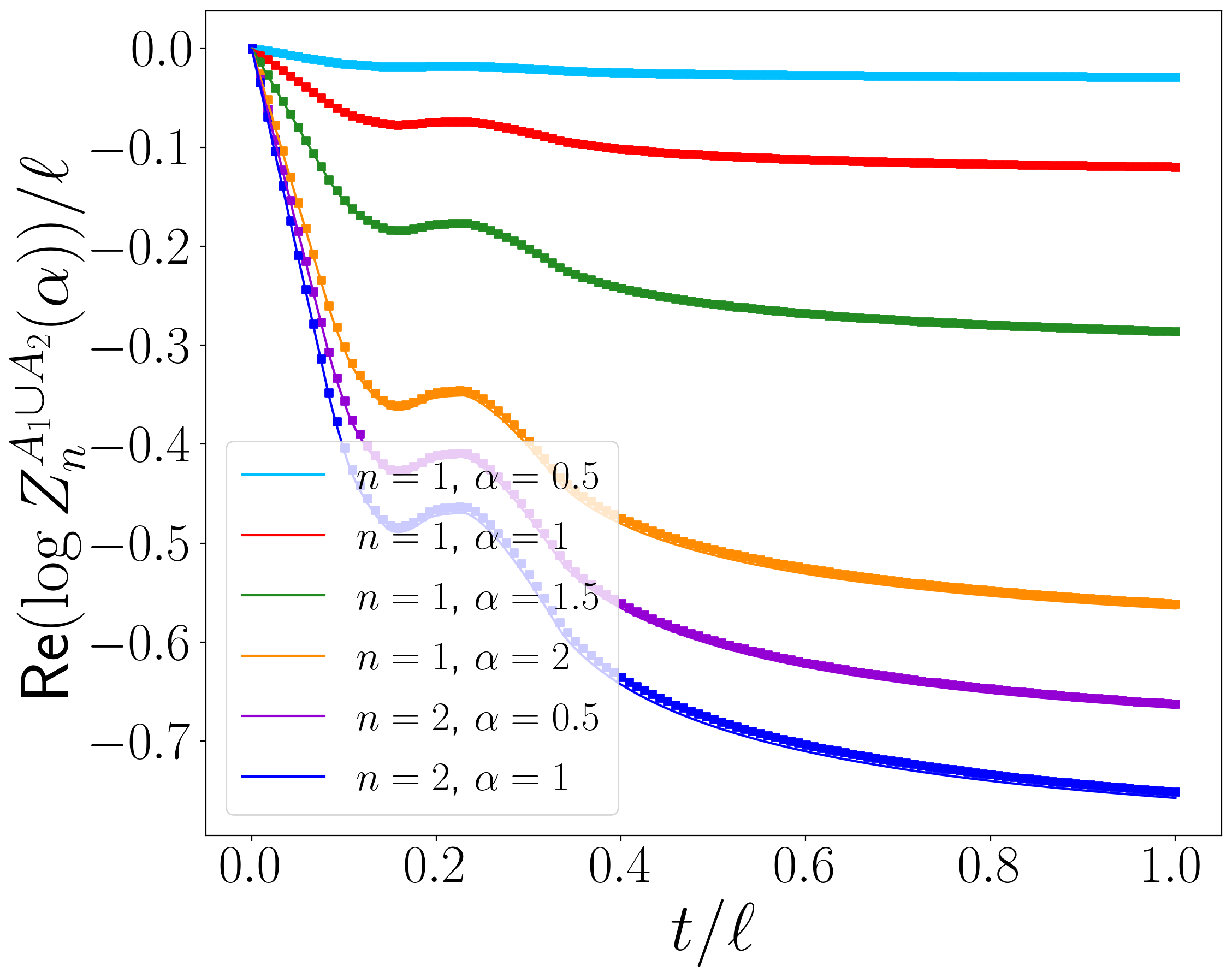
Figure 8: Time evolution of the charged moments $Z_{n}^{A_{1}\cup A_{2}}(\alpha)$ after a quench from the Néel state in the tight-binding model (3.1) as a function of $t/\ell$ with $\ell_{1}=100$, $\ell_{2}=140$ and $d=80$. The analytical prediction of Eq. (4.33) (solid lines) perfectly matches the numerical data (symbols).

4.2.2 Fourier transform and symmetry resolved Rényi entropies

The calculations for the symmetry resolved moments and Rényi entropies are exactly the same as the computations of Secs. 4.1.2 and 4.1.3 where $\mathcal{J}$ is systematically replaced by $\mathcal{J}_{d}$. We thus have

$$\begin{split}S_{n}^{A_{1}\cup A_{2}}(q)=\mathcal{J}_{d}\log 2+\log\mathcal{Z}_{1}^{A_{1}\cup A_{2}}(q),\quad\mathcal{Z}_{1}^{A_{1}\cup A_{2}}(q)\simeq 2^{-\mathcal{J}_{d}}\frac{\Gamma(\mathcal{J}_{d}+1)}{\Gamma\big{(}\frac{\mathcal{J}_{d}+2\Delta q+2}{2}\big{)}\Gamma\big{(}\frac{\mathcal{J}_{d}-2\Delta q+2}{2}\big{)}},\end{split}$$ (4.35)

and

$$S_{n}^{A_{1}\cup A_{2}}(q)=\mathcal{J}_{d}\left(\log 2-2\Big{(}\frac{\Delta q}{\mathcal{J}_{d}}\Big{)}^{2}\right),\quad\mathcal{Z}_{1}^{A_{1}\cup A_{2}}(q)\simeq\sqrt{\frac{2}{\mathcal{J}_{d}\pi}}\mathsf{e}^{-\frac{2\Delta q^{2}}{\mathcal{J}_{d}}},$$ (4.36)

in the limit where $\ell$ is large and $\mathcal{J}_{d}\gg|\Delta q|$. We do not report numerical tests for these symmetry resolved entropies because they do not to add any information compared to the single interval case.

4.2.3 Symmetry resolved mutual information

We now turn to the computation of the symmetry resolved mutual information defined as in Eq. (2.9). The first step is to compute $Z_{1}^{A_{1}:A_{2}}(\alpha,\beta)$. To do so, we compute the trace of powers of the matrix $J_{\alpha\beta}$ in Eq. (3.17). We adapt the calculations of Sec. 4.2.1 for the trace of $J_{A_{1}\cup A_{2}}$ and find

$$\begin{split}\text{Tr}J_{\alpha\beta}(t)^{2j}&=\Big{(}\frac{\mathsf{e}^{\mathrm{i}\alpha}-1}{\mathsf{e}^{\mathrm{i}\alpha}+1}\Big{)}^{2j}\Big{[}\ell_{1}-\int\frac{\mathrm{d}k}{2\pi}\min(\ell_{1},2v_{k}t)\Big{]}\\ &+\Big{(}\frac{\mathsf{e}^{\mathrm{i}\beta}-1}{\mathsf{e}^{\mathrm{i}\beta}+1}\Big{)}^{2j}\Big{[}\ell_{2}-\int\frac{\mathrm{d}k}{2\pi}\min(\ell_{2},2v_{k}t)\Big{]}\\ +(-1)^{j}\Big{(}\tan\frac{\alpha}{2}\tan\frac{\beta}{2}\Big{)}^{j}\int\frac{\mathrm{d}k}{2\pi}&[\max(d,2v_{k}t)+\max(d+\ell,2v_{k}t)-\max(d+\ell_{1},2v_{k}t)-\max(d+\ell_{2},2v_{k}t)],\\[14.22636pt] \text{Tr}J_{\alpha\beta}(t)^{2j+1}&=0.\end{split}$$ (4.37)

The re-summation in Eq. (3.18) is direct and we find

$$\begin{split}\log Z_{1}^{A_{1}:A_{2}}(\alpha,\beta)&=\mathrm{i}\frac{\ell_{1}\alpha+\ell_{2}\beta}{2}+\log\Big{(}\cos\frac{\alpha}{2}\Big{)}\mathcal{J}_{A_{1}}+\log\Big{(}\cos\frac{\beta}{2}\Big{)}\mathcal{J}_{A_{2}}\\ &+\frac{1}{2}\log\Big{(}1+\tan\frac{\alpha}{2}\tan\frac{\beta}{2}\Big{)}(\mathcal{J}_{A_{1}}+\mathcal{J}_{A_{2}}-\mathcal{J}_{d})\end{split}$$ (4.38)

where $\mathcal{J}_{d}$ is given in Eq. (4.34) and the straightforward notation $\mathcal{J}_{A_{1,2}}=\mathcal{J}|_{\ell\to\ell_{1,2}}=\int\frac{\mathrm{d}k}{2\pi}\min(\ell_{1,2},2v_{k}t)$. As a consistency check, $Z_{1}^{A_{1}:A_{2}}(\alpha,\alpha)$ is equal to the charged moment $Z_{1}^{A_{1}\cup A_{2}}(\alpha)$ given in Eq. (4.33). We compare the prediction of Eq. (4.38) with numerical results in Fig. 9 and find a perfect agreement.

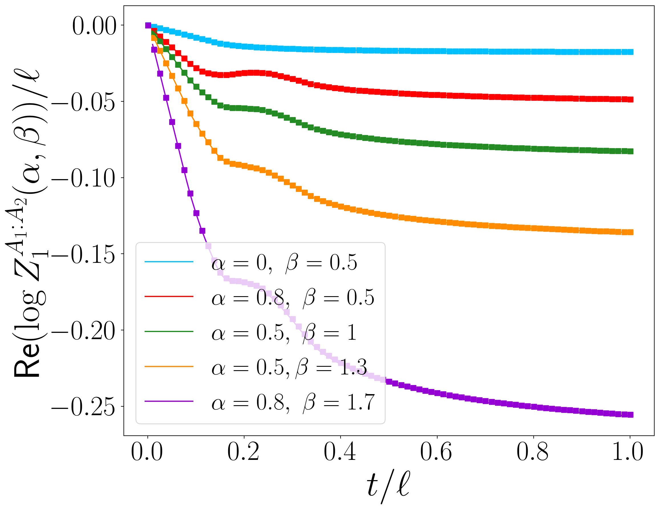
Figure 9: Time evolution of $Z_{1}^{A_{1}:A_{2}}(\alpha,\beta)$ after a quench from the Néel state in the tight-binding model (3.1) as a function of $t/\ell$ with $\ell_{1}=100$, $\ell_{2}=140$ and $d=80$. The analytical prediction of Eq. (4.38) (solid lines) perfectly matches the numerical data (symbols).

To perform the double Fourier transform in Eq. (2.12) for $\mathcal{Z}_{1}^{A_{1}:A_{2}}(q_{1},q-q_{1})$, we exploit the saddle point approximation and expand $Z_{1}^{A_{1}:A_{2}}(\alpha,\beta)$ at quadratic order, obtaining

$$\log Z_{1}^{A_{1}:A_{2}}(\alpha,\beta)=\mathrm{i}\frac{\ell_{1}\alpha+\ell_{2}\beta}{2}-\frac{\alpha^{2}}{8}\mathcal{J}_{A_{1}}-\frac{\beta^{2}}{8}\mathcal{J}_{A_{2}}+\frac{\alpha\beta}{8}(\mathcal{J}_{A_{1}}+\mathcal{J}_{A_{2}}-\mathcal{J}_{d}).$$ (4.39)

In this approximation, the Fourier transform is given as

$$\mathcal{Z}_{1}^{A_{1}:A_{2}}(q_{1},q-q_{1})=\frac{2}{\pi\sqrt{\mathcal{J}_{A_{1}}\mathcal{J}_{A_{2}}-\frac{\mathcal{J}_{m}^{2}}{4}}}\mathsf{e}^{-\frac{8}{4\mathcal{J}_{A_{1}}\mathcal{J}_{A_{2}}-\mathcal{J}_{m}^{2}}\Big{[}\Delta q_{1}^{2}\mathcal{J}_{A_{2}}+(\Delta q-\Delta q_{1})^{2}\mathcal{J}_{A_{1}}+\Delta q_{1}(\Delta q-\Delta q_{1})\mathcal{J}_{m}\Big{]}}$$ (4.40)

where we have introduced $\mathcal{J}_{m}=(\mathcal{J}_{A_{1}}+\mathcal{J}_{A_{2}}-\mathcal{J}_{d})$ to lighten the notations, and we have $\Delta q=q-\ell/2$ and $\Delta q_{1}=q_{1}-\ell_{1}/2$. Importantly, the weight $p(q_{1},q-q_{1})=\mathcal{Z}_{1}^{A_{1}:A_{2}}(q_{1},q-q_{1})/\mathcal{Z}_{1}^{A_{1}\cup A_{2}}(q)$ defined in Eq. (2.10) satisfies $\sum_{q_{1}=0}^{q}p(q_{1},q-q_{1})=1$ also when the sum is approximated as an integral and the quantities are given by their Gaussian approximations of Eqs. (4.36) and (4.40).

Using the Gaussian expression for each term involved in the definition of Eq. (2.9) and the same type of asymptotic calculations as in the previous sections, we find

$$\begin{split}I^{A_{1}:A_{2}}_{1}(q)&=(\mathcal{J}_{A_{1}}+\mathcal{J}_{A_{2}}-\mathcal{J}_{d})\log 2-\frac{1}{2}\Big{(}\log\frac{\mathcal{J}_{A_{1}}\mathcal{J}_{A_{2}}\pi}{2\mathcal{J}_{d}}\Big{)}-\frac{4\mathcal{J}_{A_{1}}\mathcal{J}_{A_{2}}-\mathcal{J}_{m}^{2}}{8\mathcal{J}_{d}}\Big{(}\frac{1}{\mathcal{J}_{A_{1}}}+\frac{1}{\mathcal{J}_{A_{2}}}\Big{)}\\ &-2\Delta q^{2}\Big{\{}\Big{(}\frac{-\mathcal{J}_{A_{1}}+\mathcal{J}_{A_{2}}-\mathcal{J}_{d}}{2\mathcal{J}_{d}}\Big{)}^{2}\frac{1}{\mathcal{J}_{A_{1}}}+\Big{(}\frac{\mathcal{J}_{A_{1}}-\mathcal{J}_{A_{2}}-\mathcal{J}_{d}}{2\mathcal{J}_{d}}\Big{)}^{2}\frac{1}{\mathcal{J}_{A_{2}}}-\frac{1}{\mathcal{J}_{d}}\Big{\}}.\end{split}$$ (4.41)

Eq. (4.41) implies that at the leading order there is equipartition of the symmetry resolved mutual information. Furthermore, for $t<d/4$ and in the limit $t\to\infty$, the subleading term vanishes, because $\mathcal{J}_{d}=\mathcal{J}_{A_{1}}+\mathcal{J}_{A_{2}}$ in these two regimes, and the equipartition is broken at higher order. In Fig. 10 we compare the prediction (4.41) (solid lines) with the ab-initio calculation of Eq. (2.9) where the entropies have been replaced by their expressions in terms of Gamma functions, and the weights are replaced by their Gaussian expressions (symbols). We find a perfect agreement between asymptotic prediction and exact numerics. The slight negative values for early times arise from the term $-\frac{1}{2}\log\frac{\mathcal{J}_{A_{1}}\mathcal{J}_{A_{2}}\pi}{2\mathcal{J}_{d}}$ in Eq. (4.41). This term is at most of order $\log\ell$ and is negligible in the scaling limit. For intermediate times, the equipartition is broken at order $\Delta q^{2}/\ell$.

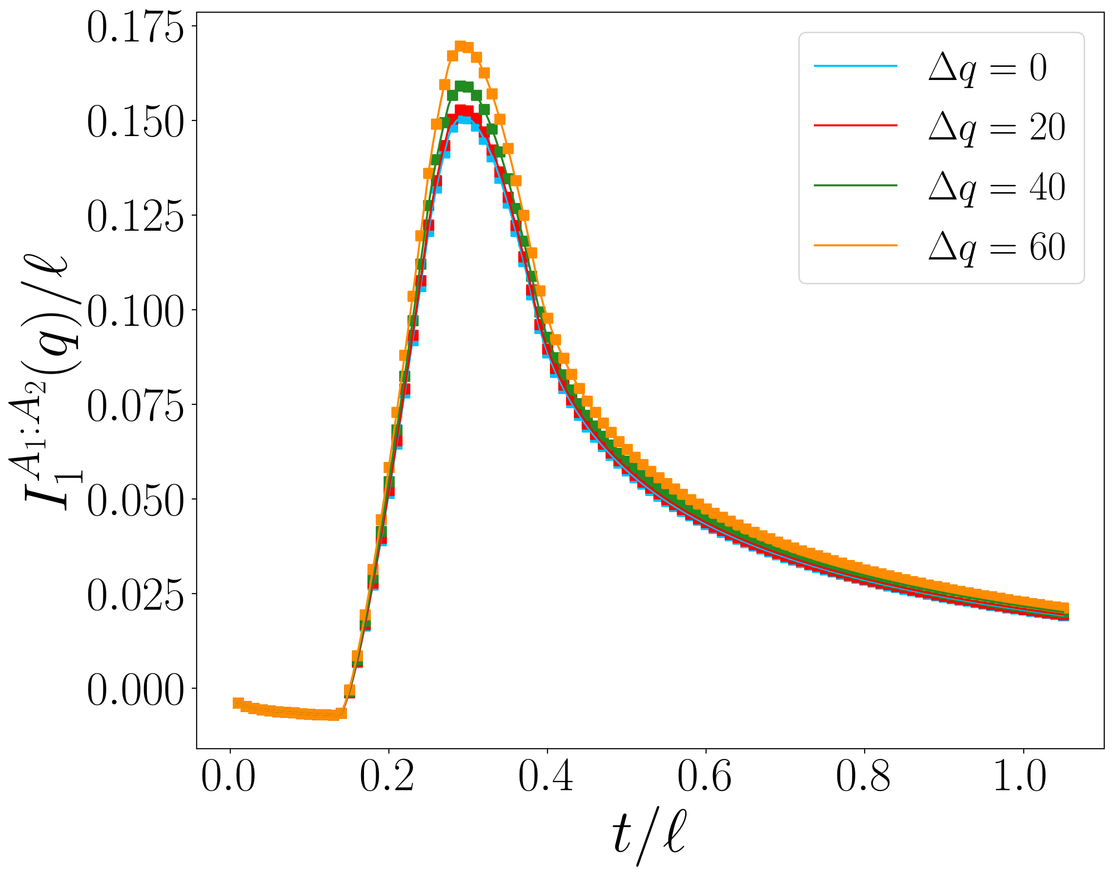
Figure 10: Time evolution of $I^{A_{1}:A_{2}}_{1}(q)$ after a quench from the Néel state in the tight-binding model (3.1) as a function of $t/\ell$ with $\ell_{1}=180$, $\ell_{2}=220$ and $d=220$ for various values of $\Delta q$. We compare the approximation of Eq. (4.41) (solid lines) with the exact result given by Eq. (2.9) where the entropies are replaced by their exact formulas of the form of Eq. (4.20) and the weights are given by their Gaussian approximations (symbols).

The leading term in Eq. (4.41) is the total mutual information,

$$\begin{split}I^{A_{1}:A_{2}}_{1}&=(\mathcal{J}_{A_{1}}+\mathcal{J}_{A_{2}}-\mathcal{J}_{d})\log 2\\ &=\log 2\int\frac{\mathrm{d}k}{2\pi}[\max(d,2v_{k}t)+\max(d+\ell,2v_{k}t)-\max(d+\ell_{1},2v_{k}t)-\max(d+\ell_{2},2v_{k}t)].\end{split}$$ (4.42)

This immediately follow from the definition of Eq. (1.3) and the exact results of Eqs. (4.20) and (4.36) for the entanglement entropies. This integral is precisely the form predicted by the quasiparticle picture for the spreading of entanglement between two non-complementary subsystems [24]. It is vanishing for times $t<d/4$ as well as in the large-time limit. To verify the consistency of our calculations, we must recover the total mutual information from the symmetry resolved ones with the combination given in Eq. (2.13). Using the same Gaussian results as before, Eq. (4.41) and the asymptotic result for the number entropy of Eq. (4.24), we indeed find

$$\sum_{q=0}^{\ell}\mathcal{Z}_{1}^{A_{1}\cup A_{2}}(q)I^{A_{1}:A_{2}}_{1}(q)+S^{A_{1},n}+S^{A_{2},n}-S^{A_{1}\cup A_{2},n}=(\mathcal{J}_{A_{1}}+\mathcal{J}_{A_{2}}-\mathcal{J}_{d})\log 2.$$ (4.43)

5 Quench from the dimer state

For the quench from the dimer state $|D\rangle$ (cf. Eq. (3.19)) in the tight binding model, the starting point is also the correlation matrix. For this quench, it is convenient to write it in a block form as follows (see e.g. [90]):

$$[C(t)]_{j,k}=\Big{\langle}\begin{pmatrix}c_{2j-1}^{\dagger}\\ c_{2j}^{\dagger}\end{pmatrix}\begin{pmatrix}c_{2k-1}&c_{2k}\end{pmatrix}\Big{\rangle}=\frac{1}{2}\big{(}\delta_{j,k}\mathbb{I}_{2}+\Pi_{k-j}\big{)}$$ (5.1)

where $\Pi_{m}$ is

$$\Pi_{m}=\int_{-\pi}^{\pi}\frac{\mathrm{d}k}{2\pi}\mathsf{e}^{-2\mathrm{i}mk}\ \begin{pmatrix}-f(k,t)&-g(k,t)\\ -g(k,t)^{*}&f(k,t)\\ \end{pmatrix}$$ (5.2)

with

$$\begin{split}f(k,t)&=\sin k\sin(4\cos(k)t),\\ g(k,t)&=\mathsf{e}^{-\mathrm{i}k}(\cos k+\mathrm{i}\sin k\cos(4\cos(k)t)).\end{split}$$ (5.3)

5.1 Single interval

Similarly to the Néel quench, we start by considering the case where $A$ is a block of $\ell$ consecutive sites. The correlation matrix $C_{A}(t)=\frac{1}{2}(\mathbb{I}_{\ell}+J_{A}(t))$ is the $\ell\times\ell$ matrix whose entries are $[C(t)]_{j,k}$ given in Eq. (5.1) with $j,k\in\{1,\dots,\ell/2\}$.

5.1.1 Charged moments

We compute the trace of $J_{A}(t)^{m}$ in the scaling limit where $t,\ell~{}\to~{}\infty$ with a fixed finite ratio. The computation is exactly the same as in [87] and we find

$$\text{Tr}J_{A}(t)^{2j}=\ell-\int\frac{\mathrm{d}k}{2\pi}(1-[\cos k]^{2j})\min(\ell,2v_{k}t),\quad\text{Tr}J_{A}(t)^{2j+1}=0$$ (5.4)

with $v_{k}=2|\sin k|$. As for the quench from the Néel state, the maximal velocity is $v_{M}=2$. We evaluate the sum (3.7) with (5.4) and find

$$\log Z_{n}(\alpha)=\mathrm{i}\ell\frac{\alpha}{2}+\int\frac{\mathrm{d}k}{2\pi}\mathrm{Re}[h_{n,\alpha}(\cos k)]\min(\ell,2v_{k}t)$$ (5.5)

where $h_{n,\alpha}(x)$ is given in Eq. (3.6). This result is very similar to Eq. (4.6) for the Néel quench, with the difference that the function $h_{n,\alpha}(x)$ is now evaluated in $x=\cos k$ and hence cannot be factorised out of the integral. In Fig. 11 we compare this prediction with the exact numerical data for the charged moments and find a very good agreement. As observed for the Néel quench and in many other cases, the corrections to the scaling are larger as $\alpha$ gets closer to $\pm\pi$ and as $n$ increases.

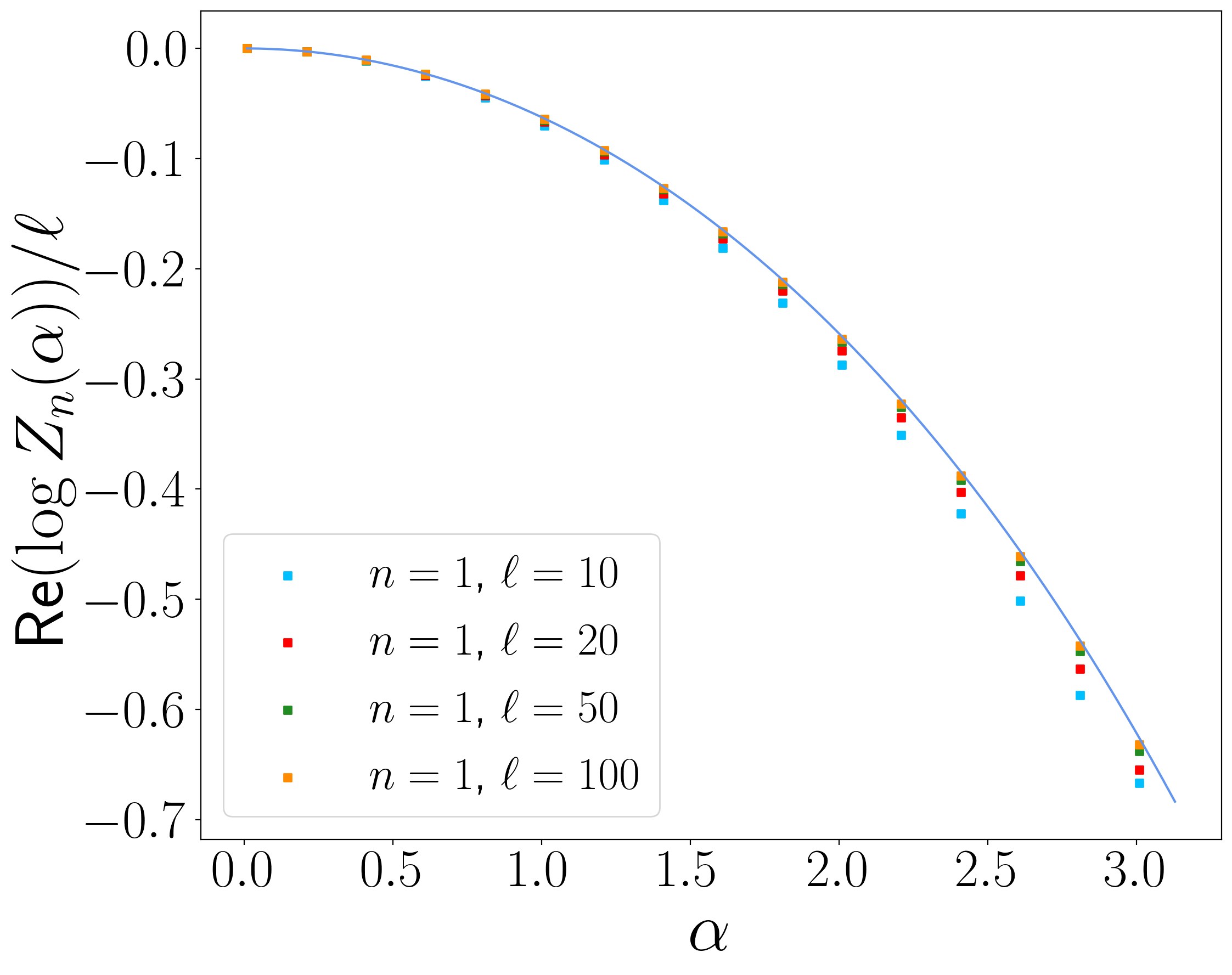
Figure 11: Comparison between the exact result (5.5) (solid lines) and numerical results (symbols) for $\log Z_{n}(\alpha)$ after a quench from the dimer state in the free fermion model (3.1). Top left: Time evolution of the real part of $\log Z_{n}(\alpha)$ as a function of $t/\ell$ with $\ell=120$. Top right: Time evolution of the imaginary part of $\log Z_{n}(\alpha)$ as a function of $t/\ell$ with $\ell=20$ and $n=1$. Bottom left: Real part of $\log Z_{n}(\alpha)$ as a function of $\ell$ with $t/\ell=0.5$. Bottom right: Real part of $\log Z_{n}(\alpha)$ as a function of $\alpha$ with $t/\ell=0.5$ and $n=1$.

5.1.2 Fourier transform and symmetry resolved Rényi entropies

The symmetry resolved moments $\mathcal{Z}_{n}(q)$ with $q=\Delta q+\langle Q_{A}\rangle$ are defined in Eq. (2.6). With Eq. (5.5) and $\langle Q_{A}\rangle=\ell/2$, we have

$$\mathcal{Z}_{n}(q)=\int\frac{\mathrm{d}\alpha}{2\pi}\mathsf{e}^{-\mathrm{i}\alpha\Delta q+\int\frac{\mathrm{d}k}{2\pi}\mathrm{Re}[h_{n,\alpha}(\cos k)]\min(\ell,2v_{k}t)}.$$ (5.6)

Contrarily to the Néel quench, there is no closed-form expression similar to Eq. (4.10) for this integral. We can nonetheless infer the validity of our two main results, namely the existence of a time delay that grows linearly in $|\Delta q|$ for small values of $|\Delta q|$, and an effective equipartition of entanglement broken at order $(\Delta q)^{2}/\ell$.

For the delay, we analyse Eq. (5.6) with the saddle point approximation in the regime where $2v_{M}t<\ell$. The saddle point equation is

$$-\mathrm{i}\Delta q+\mathrm{i}t\int\frac{\mathrm{d}k}{2\pi}\partial_{\mathrm{i}\alpha}\big{(}\mathrm{Re}[h_{n,\alpha}(\cos k)]\big{)}2v_{k}=0$$ (5.7)

and admits a solution for imaginary $\alpha$ only. In that case, the integral $\int\frac{\mathrm{d}k}{2\pi}\partial_{\mathrm{i}\alpha}\big{(}\mathrm{Re}[h_{n,\alpha}(\cos k)]\big{)}2v_{k}$ is a monotonic function of $\mathrm{i}\alpha$, going from $4/\pi$ at $\alpha=-\mathrm{i}\infty$ to $-4/\pi$ at $\alpha=\mathrm{i}\infty$. It thus follows that Eq. (5.7) only admits a solution for $t>\frac{\pi|\Delta q|}{4}$. Hence we find precisely the same delay as for the Néel quench, with the same self-consistency relation $|\Delta q|<\ell/\pi$, as given in Eq. (4.15).

For the equipartition, we expand the charged moments at quadratic order in $\alpha$,

$$\log Z_{n}(\alpha)=\mathrm{i}\ell\frac{\alpha}{2}+\log Z_{n}(0)-\frac{\alpha^{2}}{8}\mathcal{J}^{(n)}$$ (5.8)

with

$$\mathcal{J}^{(n)}=\int\frac{\mathrm{d}k}{2\pi}j_{n}(k)\ \text{min}\big{(}\ell,2v_{k}t\big{)}$$ (5.9)

where

$$j_{n}(k)=\frac{4\sin^{2n}k}{((1+\cos k)^{n}+(1-\cos k)^{n})^{2}}.$$ (5.10)

In the following, we also need the value of the derivative of $j_{n}(k)$ with respect to $n$ at $n=1$. It reads

$$(\partial_{n}j_{n}(k))|_{n=1}=[-(1-\cos k)\log(1-\cos k)-(1+\cos k)\log(1+\cos k)+2\log\sin k]\sin^{2}k.$$ (5.11)

These $\mathcal{J}^{(n)}$ integrals generalise $\mathcal{J}$ of Eq. (4.8). In particular, we have $\mathcal{J}^{(0)}=\mathcal{J}$. With this quadratic expansion, we compute the Fourier transform and find

$$\mathcal{Z}_{n}(q)=Z_{n}(0)\mathsf{e}^{-\frac{2\Delta q^{2}}{\mathcal{J}^{(n)}}}\sqrt{\frac{2}{\pi\mathcal{J}^{(n)}}}.$$ (5.12)

Plugging this result in Eq. (2.7), we find at leading order

$$S_{n}(q)=S_{n}-\frac{2\Delta q^{2}}{(1-n)}\Big{\{}\frac{1}{\mathcal{J}^{(n)}}-\frac{n}{\mathcal{J}^{(1)}}\Big{\}}$$ (5.13)

where we used that $\log Z_{1}(0)=0$ and the total entropy is $S_{n}=\frac{1}{1-n}\log Z_{n}(0)$. The symmetry resolved entanglement entropy is obtained as the limit $n\to 1$ of Eq. (5.13), and reads

$$S_{1}(q)=S_{1}-\frac{2\Delta q^{2}}{\mathcal{J}^{(1)}}\Big{\{}\frac{(\partial_{n}\mathcal{J}^{(n)})|_{n=1}}{\mathcal{J}^{(1)}}+1\Big{\}}$$ (5.14)

where $S_{1}=-(\partial_{n}Z_{n}(0))|_{n=1}$. Equations (5.13) and (5.14) are physically equivalent to Eq. (4.21). Similarly to the case of a quench from the Néel state, the match with the numerical data is better when we include the sub-leading terms that arise from the square root in Eq. (5.12). The result reads

$$S_{n}(q)=S_{n}-\frac{2\Delta q^{2}}{(1-n)}\Big{\{}\frac{1}{\mathcal{J}^{(n)}}-\frac{n}{\mathcal{J}^{(1)}}\Big{\}}+\frac{1}{2}\log\frac{2}{\pi}-\frac{1}{2(1-n)}\log\frac{\mathcal{J}^{(n)}}{(\mathcal{J}^{(1)})^{n}}$$ (5.15)

and the limit $n\to 1$ is

$$S_{1}(q)=S_{1}-\frac{2\Delta q^{2}}{\mathcal{J}^{(1)}}\Big{\{}\frac{(\partial_{n}\mathcal{J}^{(n)})|_{n=1}}{\mathcal{J}^{(1)}}+1\Big{\}}+\frac{1}{2}\log\frac{2}{\pi}+\frac{1}{2}\Big{(}\frac{(\partial_{n}\mathcal{J}^{(n)})|_{n=1}}{\mathcal{J}^{(1)}}-\log\mathcal{J}^{(1)}\Big{)}.$$ (5.16)

We compare these predictions with ab-initio results in Fig. 12. As expected, the delay is not well reproduced by the approximation for large $|\Delta q|$, but the asymptotic values match convincingly. The reason of this disagreement at intermediate times is the same as for the Néel quench and is not discussed again here. In the same figure we report the delays for $S_{1}(q)$ and $S_{2}(q)$ and compare them with the prediction $t_{D}=\frac{\pi|\Delta q|}{4}$. For $S_{1}(q)$, the match is perfect. We expect that finite-size effects play an increasing role for larger values of $n$ and $|\Delta q|$, and indeed the match is less precise for $S_{2}(q)$ at large $|\Delta q|$.

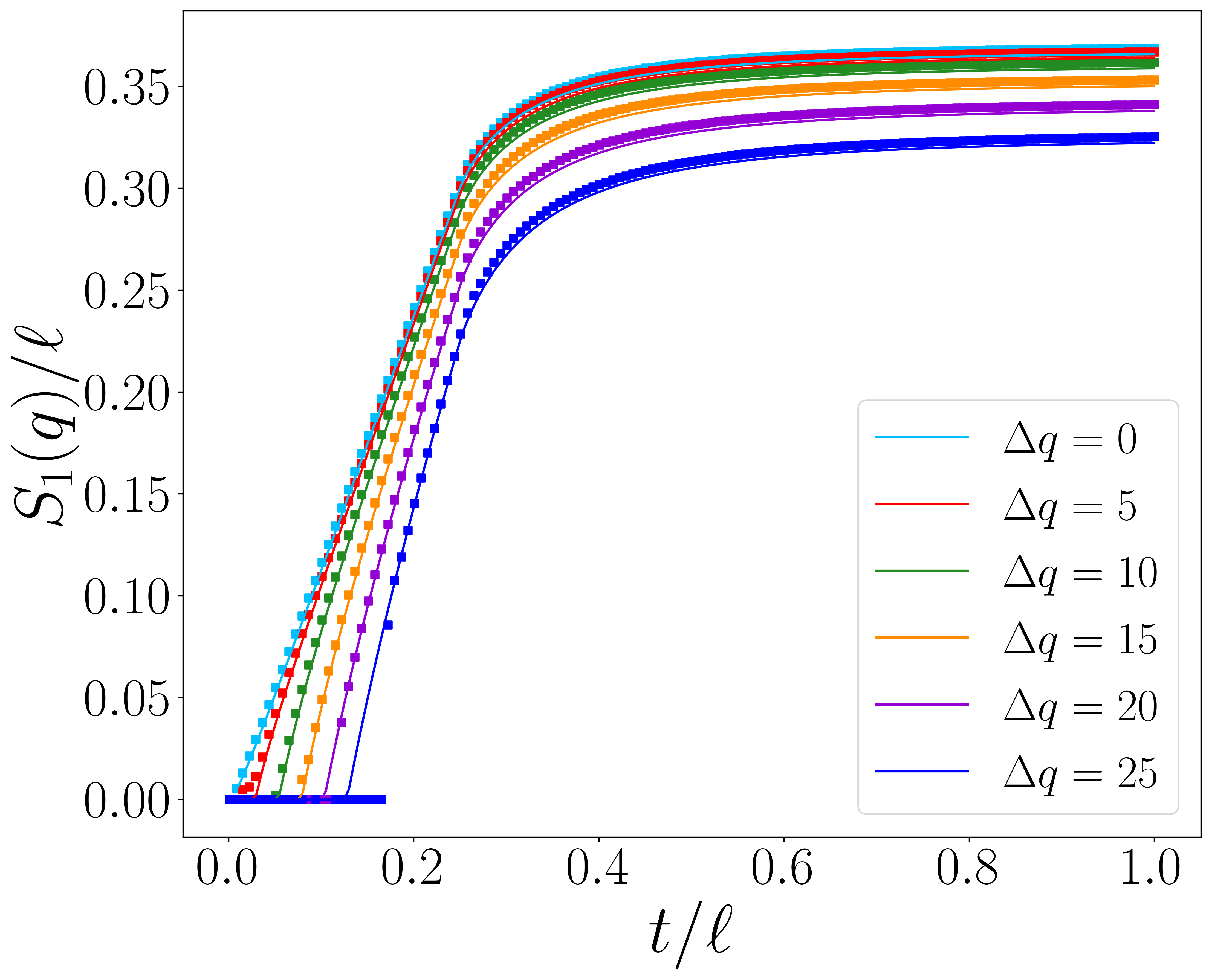
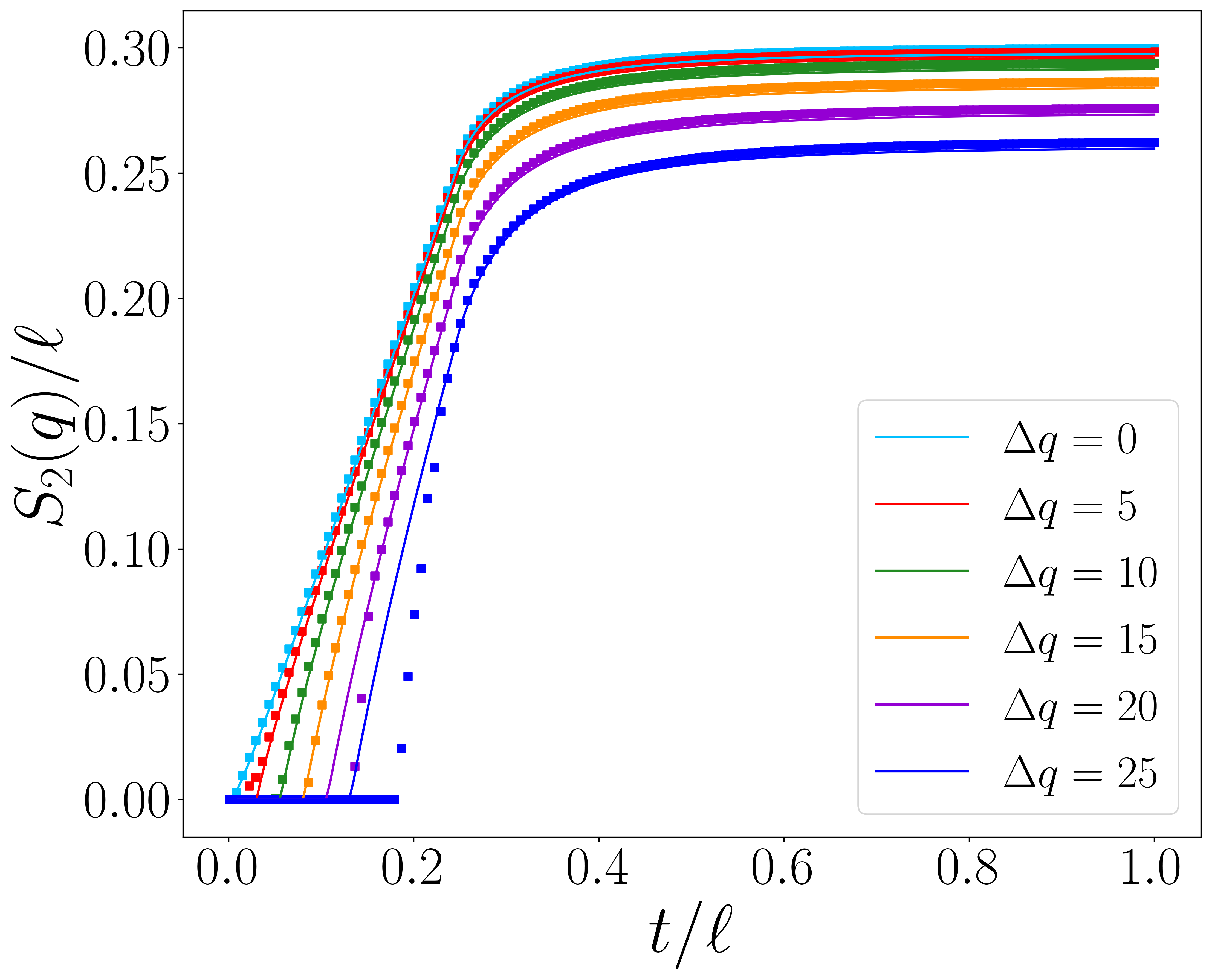
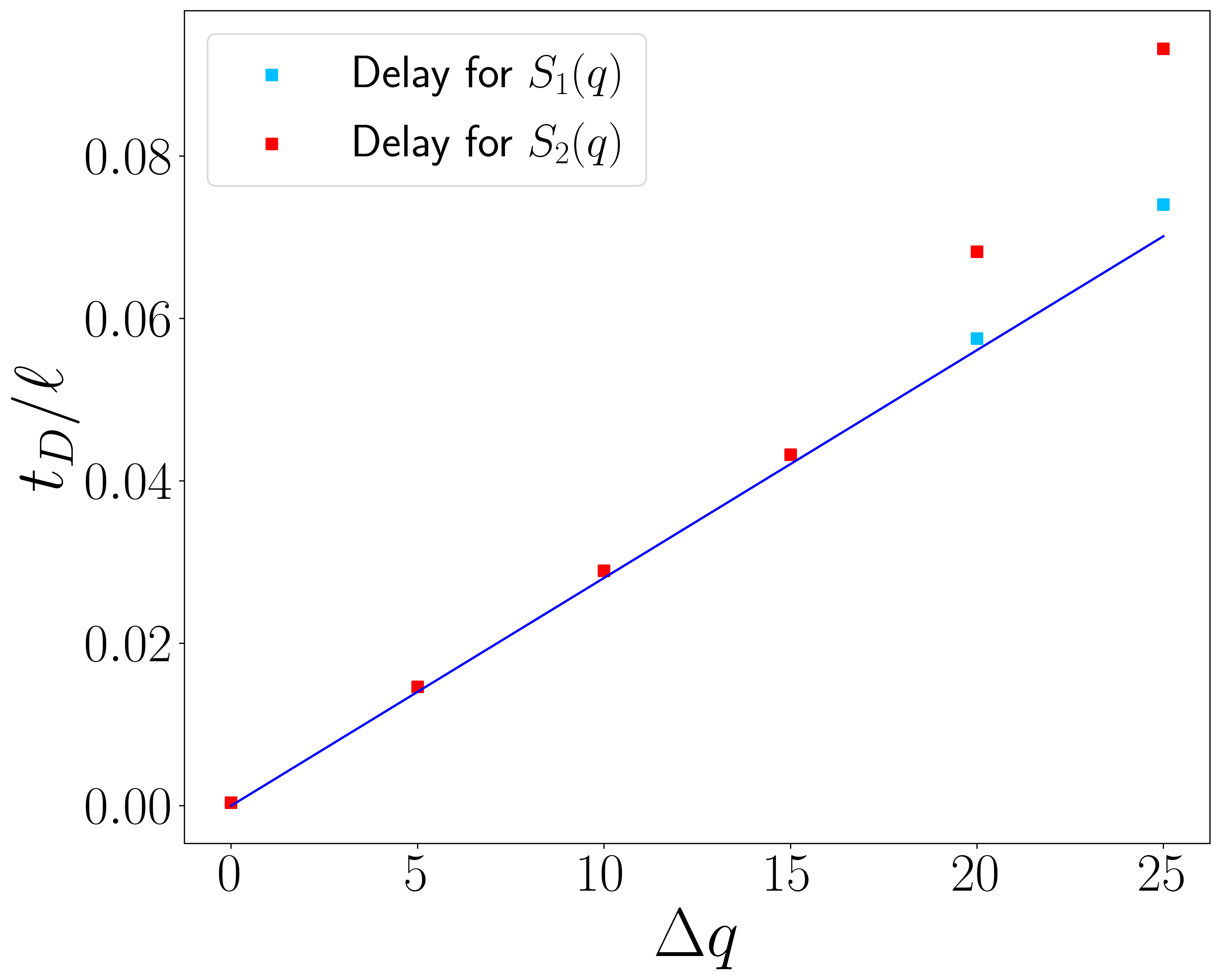
Figure 12: Top: Time evolution of the symmetry resolved entropies $S_{1}(q)$ and $S_{2}(q)$ after a quench from the dimer state in the tight-binding model (3.1) for $\ell=140$ and various $\Delta q$. We compare the predictions of Eqs. (5.15) and (5.16) (solid lines) with numerical data (symbols). Bottom: Delay time $t_{D}$ for various $\Delta q$ and $\ell=280.$ The solid line is the analytic prediction $t_{D}=\frac{\pi|\Delta q|}{4}$ and the symbols are the numerical results. They are obtained as the time for which $S_{1,2}(q)/\ell=0.01$.

5.1.3 Total and number entropy

The total entropies are given by $S_{n}=\frac{1}{1-n}\log Z_{n}(0)$. With Eq. (5.5) we have

$$S_{n}=\frac{1}{1-n}\int\frac{\mathrm{d}k}{2\pi}h_{n,0}(\cos k)\min(\ell,2v_{k}t)$$ (5.17)

where

$$h_{n,0}(\cos k)=\log\left[\left(\frac{1+\cos k}{2}\right)^{n}+\left(\frac{1-\cos k}{2}\right)^{n}\right]$$ (5.18)

is a specialisation of Eq. (3.6). The term $n_{k}=\frac{1+\cos k}{2}$ is the mode occupation in the steady state. The limit $n\to 1$ yields

$$S_{1}=\int\frac{\mathrm{d}k}{2\pi}(-n_{k}\log n_{k}-(1-n_{k})\log(1-n_{k}))\min(\ell,2v_{k}t)$$ (5.19)

that matches the quasiparticle prediction [32, 33]. As in the case of a quench from the Néel state, we recover the total entanglement entropy $S_{1}$ from the symmetry resolved quantities using Eq. (2.2). To see this, we plug the Gaussian approximations (5.12) and (5.16) into Eq. (2.2) and find

$$S_{1}=-(\partial_{n}Z_{n}(0))|_{n=1}+\frac{(\partial_{n}\mathcal{J}^{(n)})|_{n=1}}{\mathcal{J}^{(1)}}\Big{(}\frac{1}{2}-\sqrt{\frac{2}{\pi\mathcal{J}^{(1)}}}\sum_{q=0}^{\ell}\frac{2\Delta q^{2}}{\mathcal{J}^{(1)}}\mathsf{e}^{-\frac{2\Delta q^{2}}{\mathcal{J}^{(1)}}}\Big{)}$$ (5.20)

where we also used $\sum_{q}\mathcal{Z}_{1}(q)=1$. In the large-$\ell$ limit, the sum in the right-hand side becomes a Gaussian integral. The whole parenthesis then vanishes and we recover $S_{1}=-(\partial_{n}Z_{n}(0))|_{n=1}$, as desired.

The number entropy is given in Eq. (4.22) and only depends on $\mathcal{Z}_{1}(q)$. We use the quadratic approximation (5.12) and find that the calculations are exactly the same as in Sec. 4.1.4 where $\mathcal{J}$ is replaced by $\mathcal{J}^{(1)}=\int\frac{\mathrm{d}k}{2\pi}(1-\cos^{2}k)\min(\ell,2v_{k}t).$ We thus find

$$S^{n}=\frac{1}{2}\Big{(}1+\log\frac{\mathcal{J}^{(1)}\pi}{2}\Big{)}.$$ (5.21)

In Fig. 13 we compare this result (solid lines) with ab-initio calculations of $S^{n}$ (symbols), and find perfect agreement. The inset in the left panel shows the time-evolution of $S^{n}$ in a log-linear scale. We note that $\mathcal{J}^{(1)}$ saturates to the value $\ell/2$ for large times, so that $\displaystyle\lim_{t\to\infty}S^{n}=\frac{1}{2}\Big{(}1+\log\frac{\ell\pi}{4}\Big{)}$. This asymptotic value is reported as a dotted horizontal line in the left panel of Fig. 13. Similarly to the quench from the Néel state, the number entropy grows logarithmically with time before saturation, and has negligible contribution to the total entropy in the large-time limit, $\lim_{t\to\infty}S^{n}/S_{1}=\mathcal{O}(\ell^{-1}\log\ell)$.

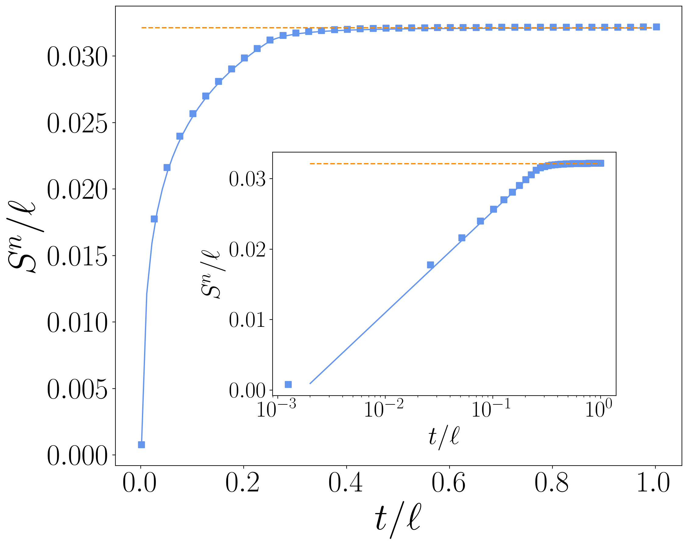
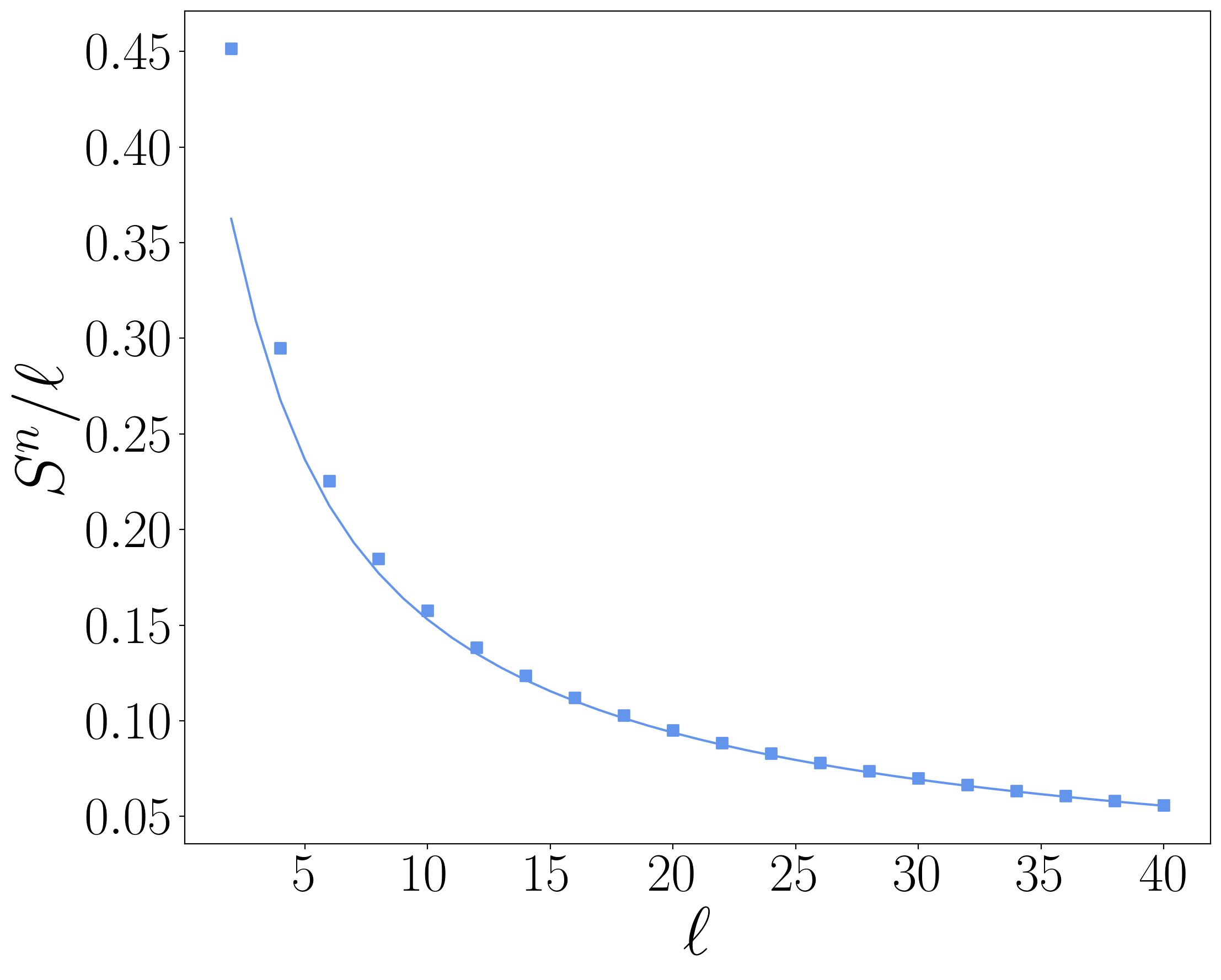
Figure 13: Evolution of $S^{n}$ after a quench from the dimer state in the tight-binding model (3.1) as a function of $t/\ell$ for $\ell=80$ (left panel), and as a function of $\ell$ with $t/\ell=1$ (right panel). The prediction (5.21) (solid line) perfectly matches the numerical results (symbols). In the left panel, the horizontal dotted line is the asymptotic value $\frac{1}{2\ell}\Big{(}1+\log\frac{\ell\pi}{4}\Big{)}$ for large times. In the same panel, the inset shows $S^{n}$ as a function of $t/\ell$ in a log-linear scale.

5.2 Disjoint intervals

We now turn to the case where the system $A$ is composed of two disjoint subsystems $A_{1}$ and $A_{2}$ of lengths $\ell_{1}$ and $\ell_{2}=\ell-\ell_{1}$ and separated by a distance $d$. The correlation matrix has the form of Eqs. (4.27) and (4.28) with the entries given in Eq. (5.1).

5.2.1 Charged moments

Similarly to the calculations of Sec. 4.2.1, we compute the trace of arbitrary powers of the matrix $J_{A_{1}\cup A_{2}}(t)=2C_{A_{1}\cup A_{2}}(t)-\mathbb{I}_{\ell}$. We perform the computation of $\text{Tr}J_{A_{1}\cup A_{2}}(t)^{m}$ in the scaling limit $t,\ell,\ell_{1},\ell_{2},d\to\infty$ where the various ratios are kept constant. We find

$$\begin{split}\text{Tr}&J_{A_{1}\cup A_{2}}(t)^{2j}=\ell-\int\frac{\mathrm{d}k}{2\pi}(1-[\cos k]^{2j})[\min(\ell_{1},2v_{k}t)+\min(\ell_{2},2v_{k}t)]\\ &+\int\frac{\mathrm{d}k}{2\pi}(1-[\cos k]^{2j})[\max(d,2v_{k}t)+\max(d+\ell,2v_{k}t)-\max(d+\ell_{1},2v_{k}t)-\max(d+\ell_{2},2v_{k}t)],\\[9.95863pt] \text{Tr}&J_{A_{1}\cup A_{2}}(t)^{2j+1}=0,\end{split}$$ (5.22)

with $v_{k}=2|\sin k|$. We note that the case $d=0$ reduces to the known result (5.4) for a single interval. The calculation is similar to case of a single interval as presented in Sec. 5.1.1, and we find

$$\begin{split}\log Z&{}^{A_{1}\cup A_{2}}_{n}(\alpha)=\mathrm{i}\ell\frac{\alpha}{2}+\int\frac{\mathrm{d}k}{2\pi}\mathrm{Re}[h_{n,\alpha}(\cos k)](\min(\ell_{1},2v_{k}t)+\min(\ell_{2},2v_{k}t))\\ &-\int\frac{\mathrm{d}k}{2\pi}\mathrm{Re}[h_{n,\alpha}(\cos k)](\max(d,2v_{k}t)+\max(d+\ell,2v_{k}t)-\max(d+\ell_{1},2v_{k}t)-\max(d+\ell_{2},2v_{k}t)).\end{split}$$ (5.23)

We compare the prediction of Eq. (5.23) for $Z_{n}^{A_{1}\cup A_{2}}(\alpha)$ with ab-initio calculations in Fig. 14 and find perfect agreement.

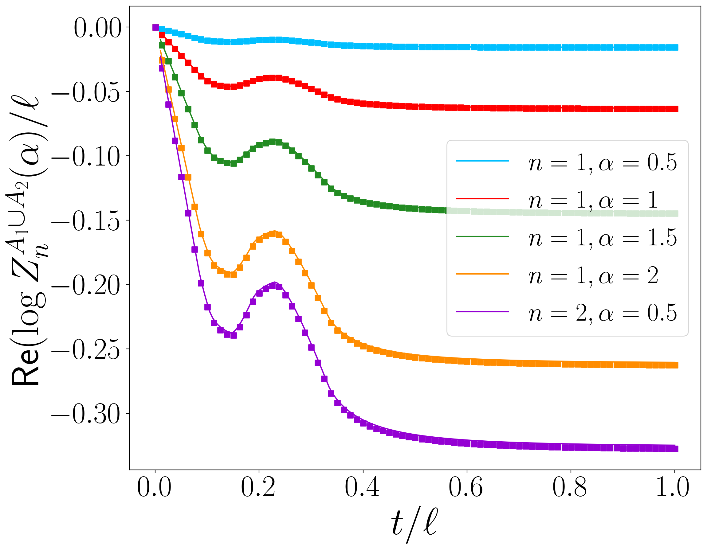
Figure 14: Time evolution of the charged moments $Z_{n}^{A_{1}\cup A_{2}}(\alpha)$ after a quench from the dimer state in the tight-binding model (3.1) as a function of $t/\ell$ with $\ell_{1}=100$, $\ell_{2}=140$ and $d=80$. The analytical prediction of Eq. (5.23) (solid lines) perfectly matches the numerical data (symbols).

5.2.2 Fourier transform and symmetry resolved Rényi entropies

In order to perform analytical calculations, we approximate $\log Z^{A_{1}\cup A_{2}}_{n}(\alpha)$ at quadratic order in $\alpha$,

$$\log Z^{A_{1}\cup A_{2}}_{n}(\alpha)=\mathrm{i}\ell\frac{\alpha}{2}+\log Z^{A_{1}\cup A_{2}}_{n}(0)-\frac{\alpha^{2}}{8}\mathcal{J}_{d}^{(n)}$$ (5.24)

with

$$\begin{split}&\mathcal{J}_{d}^{(n)}=\int\frac{\mathrm{d}k}{2\pi}j_{n}(k)(\min(\ell_{1},2v_{k}t)+\min(\ell_{2},2v_{k}t))\\ &-\int\frac{\mathrm{d}k}{2\pi}j_{n}(k)(\max(d,2v_{k}t)+\max(d+\ell,2v_{k}t)-\max(d+\ell_{1},2v_{k}t)-\max(d+\ell_{2},2v_{k}t))\end{split}$$ (5.25)

where $j_{n}(k)$ is given in Eq. (5.10). As in the case of a single interval, these $\mathcal{J}_{d}^{(n)}$ integrals generalise $\mathcal{J}_{d}$ of Eq. (4.34). In particular, we have $\mathcal{J}_{d}^{(0)}=\mathcal{J}_{d}$. We follow Sec. 5.1.2 and find

$$\mathcal{Z}^{A_{1}\cup A_{2}}_{n}(q)=Z^{A_{1}\cup A_{2}}_{n}(0)\mathsf{e}^{-\frac{2\Delta q^{2}}{\mathcal{J}_{d}^{(n)}}}\sqrt{\frac{2}{\pi\mathcal{J}_{d}^{(n)}}},$$ (5.26)

$$S^{A_{1}\cup A_{2}}_{n}(q)=S^{A_{1}\cup A_{2}}_{n}-\frac{2\Delta q^{2}}{(1-n)}\Big{\{}\frac{1}{\mathcal{J}_{d}^{(n)}}-\frac{n}{\mathcal{J}_{d}^{(1)}}\Big{\}}+\frac{1}{2}\log\frac{2}{\pi}-\frac{1}{2(1-n)}\log\frac{\mathcal{J}_{d}^{(n)}}{(\mathcal{J}_{d}^{(1)})^{n}},$$ (5.27)

for $|\Delta q|\ll\ell$. We used that $\log Z^{A_{1}\cup A_{2}}_{1}(0)=0$ and the total entropy is $S^{A_{1}\cup A_{2}}_{n}=\frac{1}{1-n}\log Z^{A_{1}\cup A_{2}}_{n}(0)$. The symmetry resolved entanglement entropy is

$$S_{1}^{A_{1}\cup A_{2}}(q)=S^{A_{1}\cup A_{2}}_{1}-\frac{2\Delta q^{2}}{\mathcal{J}_{d}^{(1)}}\Big{\{}\frac{(\partial_{n}\mathcal{J}_{d}^{(n)})|_{n=1}}{\mathcal{J}_{d}^{(1)}}+1\Big{\}}+\frac{1}{2}\log\frac{2}{\pi}+\frac{1}{2}\Big{(}\frac{(\partial_{n}\mathcal{J}_{d}^{(n)})|_{n=1}}{\mathcal{J}_{d}^{(1)}}-\log\mathcal{J}_{d}^{(1)}\Big{)}.$$ (5.28)

5.2.3 Symmetry resolved mutual information

We now turn to the computation of the symmetry resolved mutual information after a quench from the dimer state. Most of the results and computations are similar to those presented in Sec. 4.2.3 in the case of a quench from the Néel state. The first step is to compute $Z_{1}^{A_{1}:A_{2}}(\alpha,\beta)$ and hence the trace of powers of the matrix $J_{\alpha\beta}$ defined in Eq. (3.17). We adapt the calculations of Sec. 5.2.1 for the trace of $J_{A_{1}\cup A_{2}}$ and find

$$\begin{split}\text{Tr}J_{\alpha\beta}(t)^{2j}&=\Big{(}\frac{\mathsf{e}^{\mathrm{i}\alpha}-1}{\mathsf{e}^{\mathrm{i}\alpha}+1}\Big{)}^{2j}\Big{[}\ell_{1}-\int\frac{\mathrm{d}k}{2\pi}(1-[\cos k]^{2j})\min(\ell_{1},2v_{k}t)\Big{]}\\ &+\Big{(}\frac{\mathsf{e}^{\mathrm{i}\beta}-1}{\mathsf{e}^{\mathrm{i}\beta}+1}\Big{)}^{2j}\Big{[}\ell_{2}-\int\frac{\mathrm{d}k}{2\pi}(1-[\cos k]^{2j})\min(\ell_{2},2v_{k}t)\Big{]}\\ +\int\frac{\mathrm{d}k}{2\pi}\xi(k,j)&[\max(d,2v_{k}t)+\max(d+\ell,2v_{k}t)-\max(d+\ell_{1},2v_{k}t)-\max(d+\ell_{2},2v_{k}t)],\\[14.22636pt] \text{Tr}J_{\alpha\beta}(t)^{2j+1}&=0,\end{split}$$ (5.29)

where

$$\xi(k,j)=\sum_{s=1}^{j}\sum_{t=0}^{2j-2s}(-1)^{t}\Big{(}\frac{\mathsf{e}^{\mathrm{i}\alpha}-1}{\mathsf{e}^{\mathrm{i}\alpha}+1}\Big{)}^{s+t}\Big{(}\frac{\mathsf{e}^{\mathrm{i}\beta}-1}{\mathsf{e}^{\mathrm{i}\beta}+1}\Big{)}^{2j-s-t}\gamma_{s,t,j}\cos k^{2j-2s}\sin k^{2s}$$ (5.30)

and

$$\gamma_{s,t,j}=\frac{sj}{(2j-s-t)(s+t)}\begin{pmatrix}2j-s-t\\ s\end{pmatrix}\begin{pmatrix}s+t\\ s\end{pmatrix}.$$ (5.31)

Let us stress that the function $\gamma_{s,t,j}$ satisfies the crucial relation

$$\sum_{t=0}^{2j-2s}(-1)^{t}\gamma_{s,t,j}=\begin{pmatrix}j\\ s\end{pmatrix}.$$ (5.32)

The re-summation in Eq. (3.18) yields the formal expression

$$\begin{split}\log Z_{1}^{A_{1}:A_{2}}(\alpha,\beta)&=\mathrm{i}\frac{\ell_{1}\alpha+\ell_{2}\beta}{2}+\int\frac{\mathrm{d}k}{2\pi}\mathrm{Re}[h_{1,\alpha}(\cos k)]\min(\ell_{1},2v_{k}t)+\int\frac{\mathrm{d}k}{2\pi}\mathrm{Re}[h_{1,\beta}(\cos k)]\min(\ell_{2},2v_{k}t)\\ &+\int\frac{\mathrm{d}k}{2\pi}\Xi(k)(\max(d,2v_{k}t)+\max(d+\ell,2v_{k}t)-\max(d+\ell_{1},2v_{k}t)-\max(d+\ell_{2},2v_{k}t))\end{split}$$ (5.33)

with the infinite sum

$$\Xi(k)=\sum_{j=1}^{\infty}\tilde{c}(2j)\xi(k,j),\quad\tilde{c}(2j)=-\frac{1}{2j},$$ (5.34)

where we recall that the coefficients $\tilde{c}(j)$ are the Taylor coefficients of the function $\tilde{h}(x)=\log[(1+x)/2]$. Despite its cumbersome form, the sum can be simplified. We find

$$\Xi(k)=-\frac{1}{2}\mathrm{Re}[h_{1,\alpha}(\cos k)+h_{1,\beta}(\cos k)-h_{1,\alpha-\beta}(\cos k)],$$ (5.35)

and hence

$$\log Z_{1}^{A_{1}:A_{2}}(\alpha,\beta)=\mathrm{i}\frac{\ell_{1}\alpha+\ell_{2}\beta}{2}+\int\frac{\mathrm{d}k}{2\pi}\mathrm{Re}[h_{1,\alpha}(\cos k)]\min(\ell_{1},2v_{k}t)+\int\frac{\mathrm{d}k}{2\pi}\mathrm{Re}[h_{1,\beta}(\cos k)]\min(\ell_{2},2v_{k}t)\\ -\frac{1}{2}\int\frac{\mathrm{d}k}{2\pi}\mathrm{Re}[h_{1,\alpha}(\cos k)+h_{1,\beta}(\cos k)-h_{1,\alpha-\beta}(\cos k)](\max(d,2v_{k}t)\\ +\max(d+\ell,2v_{k}t)-\max(d+\ell_{1},2v_{k}t)-\max(d+\ell_{2},2v_{k}t)).$$ (5.36)

It is direct to show that $Z_{1}^{A_{1}:A_{2}}(\alpha,\alpha)$ in Eq. (5.36) reduces to $Z_{1}^{A_{1}\cup A_{2}}(\alpha)$ given in Eq. (5.23), as expected. Moreover, replacing $\cos k$ by $0$ in Eq. (5.36) yields the result of Eq. (4.38) for the quench from the Néel state. We compare the prediction of Eq. (5.36) with ab-initio calculations in Fig. 15 and find perfect agreement.

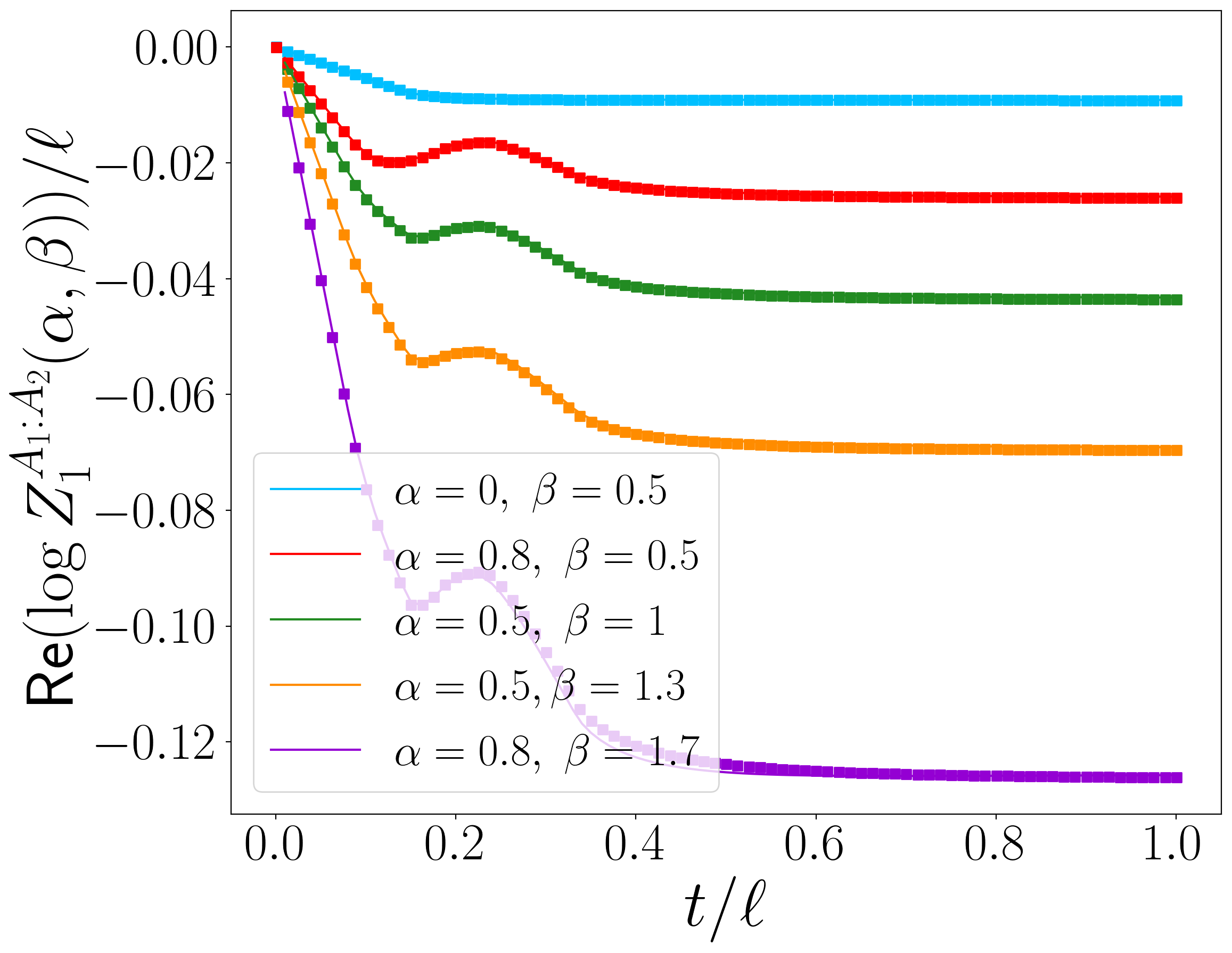
Figure 15: Time evolution of $Z_{1}^{A_{1}:A_{2}}(\alpha,\beta)$ after a quench from the dimer state in the tight-binding model (3.1) as a function of $t/\ell$ with $\ell_{1}=100$, $\ell_{2}=140$ and $d=80$. The analytical prediction of Eq. (5.36) (solid lines) perfectly matches the numerical data (symbols).

To proceed, we expand $Z_{1}^{A_{1}:A_{2}}(\alpha,\beta)$ at quadratic order in $\alpha$ and $\beta$. We find

$$\log Z_{1}^{A_{1}:A_{2}}(\alpha,\beta)=\mathrm{i}\frac{\ell_{1}\alpha+\ell_{2}\beta}{2}-\frac{\alpha^{2}}{8}\mathcal{J}^{(1)}_{A_{1}}-\frac{\beta^{2}}{8}\mathcal{J}^{(1)}_{A_{2}}+\frac{\alpha\beta}{8}(\mathcal{J}^{(1)}_{A_{1}}+\mathcal{J}^{(1)}_{A_{2}}-\mathcal{J}^{(1)}_{d}),$$ (5.37)

and the double Fourier transform is

$$\mathcal{Z}_{1}^{A_{1}:A_{2}}(q_{1},q-q_{1})=\frac{2}{\pi\sqrt{\mathcal{J}^{(1)}_{A_{1}}\mathcal{J}^{(1)}_{A_{2}}-\frac{(\mathcal{J}^{(1)}_{m})^{2}}{4}}}\mathsf{e}^{-\frac{8}{4\mathcal{J}^{(1)}_{A_{1}}\mathcal{J}^{(1)}_{A_{2}}-(\mathcal{J}^{(1)}_{m})^{2}}\Big{[}\Delta q_{1}^{2}\mathcal{J}^{(1)}_{A_{2}}+(\Delta q-\Delta q_{1})^{2}\mathcal{J}^{(1)}_{A_{1}}+\Delta q_{1}(\Delta q-\Delta q_{1})\mathcal{J}^{(1)}_{m}\Big{]}}$$ (5.38)

with $\mathcal{J}^{(1)}_{m}=(\mathcal{J}^{(1)}_{A_{1}}+\mathcal{J}^{(1)}_{A_{2}}-\mathcal{J}^{(1)}_{d})$ to lighten the notations, where $\mathcal{J}_{A_{1,2}}^{(n)}$ is simply $\mathcal{J}^{(n)}$ from Eq. (5.9) where $\ell$ is replaced by $\ell_{1,2}$, and $\mathcal{J}_{d}^{(n)}$ is given in Eq. (5.25). We also have $\Delta q=q-\ell/2$ and $\Delta q_{1}=q_{1}-\ell_{1}/2$. These two results are the same as Eqs. (4.39) and (4.40) where the $\mathcal{J}_{s}$ integrals are systematically replaced by $\mathcal{J}_{s}^{(1)}$. In a similar fashion as for the quench from the Néel state, the weight $p(q_{1},q-q_{1})=\mathcal{Z}_{1}^{A_{1}:A_{2}}(q_{1},q-q_{1})/\mathcal{Z}_{1}^{A_{1}\cup A_{2}}(q)$ defined in Eq. (2.10) satisfies $\sum_{q_{1}=0}^{q}p(q_{1},q-q_{1})=1$.

To compute the symmetry resolved mutual information, we use Eq. (2.9) and replace each quantity by its Gaussian approximation, namely Eqs. (5.12), (5.38), (5.16) and (5.28). The calculations are similar to those of Sec. 4.2.3. We find

$$\begin{split}&I^{A_{1}:A_{2}}_{1}(q)=S_{1}^{A_{1}}+S_{1}^{A_{2}}-S_{1}^{A_{1}\cup A_{2}}-\frac{1}{2}\Big{(}\log\frac{\mathcal{J}^{(1)}_{A_{1}}\mathcal{J}^{(1)}_{A_{2}}\pi}{2\mathcal{J}^{(1)}_{d}}\Big{)}+\frac{1}{2}\Big{(}\frac{\partial_{n}(\mathcal{J}_{A_{1}}^{(n)})|_{n=1}}{\mathcal{J}^{(1)}_{A_{1}}}+\frac{\partial_{n}(\mathcal{J}_{A_{2}}^{(n)})|_{n=1}}{\mathcal{J}^{(1)}_{A_{2}}}-\frac{\partial_{n}(\mathcal{J}_{d}^{(n)})|_{n=1}}{\mathcal{J}^{(1)}_{d}}\Big{)}\\ &-\frac{4\mathcal{J}^{(1)}_{A_{1}}\mathcal{J}^{(1)}_{A_{2}}-(\mathcal{J}^{(1)}_{m})^{2}}{8\mathcal{J}^{(1)}_{d}}\Big{\{}\frac{1}{\mathcal{J}^{(1)}_{A_{1}}}\Big{(}\frac{\partial_{n}(\mathcal{J}_{A_{1}}^{(n)})|_{n=1}}{\mathcal{J}^{(1)}_{A_{1}}}+1\Big{)}+\frac{1}{\mathcal{J}^{(1)}_{A_{2}}}\Big{(}\frac{\partial_{n}(\mathcal{J}_{A_{2}}^{(n)})|_{n=1}}{\mathcal{J}^{(1)}_{A_{2}}}+1\Big{)}\Big{\}}\\ &-2\Delta q^{2}\Big{\{}\Big{(}\frac{-\mathcal{J}^{(1)}_{A_{1}}+\mathcal{J}^{(1)}_{A_{2}}-\mathcal{J}^{(1)}_{d}}{2\mathcal{J}^{(1)}_{d}}\Big{)}^{2}\Big{(}\frac{\partial_{n}(\mathcal{J}_{A_{1}}^{(n)})|_{n=1}}{(\mathcal{J}^{(1)}_{A_{1}})^{2}}+\frac{1}{\mathcal{J}^{(1)}_{A_{1}}}\Big{)}+\Big{(}\frac{\mathcal{J}^{(1)}_{A_{1}}-\mathcal{J}^{(1)}_{A_{2}}-\mathcal{J}^{(1)}_{d}}{2\mathcal{J}^{(1)}_{d}}\Big{)}^{2}\Big{(}\frac{\partial_{n}(\mathcal{J}_{A_{2}}^{(n)})|_{n=1}}{(\mathcal{J}^{(1)}_{A_{2}})^{2}}+\frac{1}{\mathcal{J}^{(1)}_{A_{2}}}\Big{)}\Big{\}}\\ &+2\Delta q^{2}\Big{(}\frac{\partial_{n}(\mathcal{J}_{d}^{(n)})|_{n=1}}{(\mathcal{J}^{(1)}_{d})^{2}}+\frac{1}{\mathcal{J}^{(1)}_{d}}\Big{)}.\end{split}$$ (5.39)

We compare this prediction with the definition of Eq. (2.9) where the various quantities are replaced by their Gaussian approximations in Fig. 16, and find a perfect match. The result of Eq. (5.39) has the same physical interpretation as Eq. (4.41), namely the first three terms of the right-hand side precisely yield the quasiparticle prediction for the total mutual information, equipartition is broken at order $\Delta q^{2}/\ell$ for intermediate times and at higher order for $t<d/4$ and $t\to\infty$, since $\mathcal{J}_{d}^{(n)}=\mathcal{J}^{(n)}_{A_{1}}+\mathcal{J}^{(n)}_{A_{2}}$ in those regimes. As for the quench from the Néel state, the combination of Eq. (2.13) yields the total mutual information, namely

$$\sum_{q=0}^{\ell}\mathcal{Z}_{1}^{A_{1}\cup A_{2}}(q)I^{A_{1}:A_{2}}_{1}(q)+S^{A_{1},n}+S^{A_{2},n}-S^{A_{1}\cup A_{2},n}=I^{A_{1}:A_{2}}_{1}$$ (5.40)

where

$$I^{A_{1}:A_{2}}_{1}=-\int\frac{\mathrm{d}k}{2\pi}\partial_{n}h_{n,0}(\cos k)|_{n=1}(\max(d,2v_{k}t)+\max(d+\ell,2v_{k}t)-\max(d+\ell_{1},2v_{k}t)-\max(d+\ell_{2},2v_{k}t)).$$ (5.41)

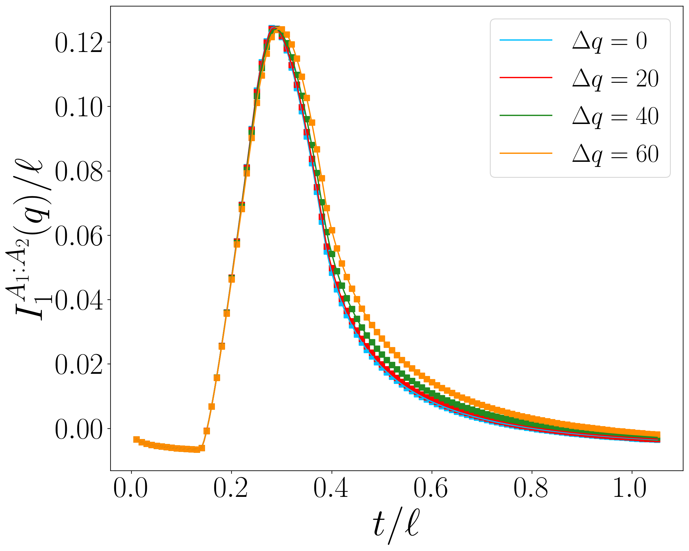
Figure 16: Time evolution of $I^{A_{1}:A_{2}}_{1}(q)$ after a quench from the dimer state in the tight-binding model (3.1) as a function of $t/\ell$ with $\ell_{1}=180$, $\ell_{2}=220$ and $d=220$ for various values of $\Delta q$. We compare the approximation of Eq. (5.39) (solid lines) with the definition of Eq. (2.9) where the various quantities are replaced by their Gaussian approximations with the first corrections (symbols).

6 Quasiparticle picture for the charged moments

In this section we use the quasiparticle picture to get general results for the dynamics of the charged moments for the entanglement entropy. On the one hand, this picture provides a physical explanation of the findings of the previous sections. On the other hand, it gives a generalisation valid for any free-fermion (or free-boson) model for arbitrary Rényi entropies. It also suggests a conjecture for the charged entropies for arbitrary interacting models, but many quantitative details are still missing and its validity should eventually be tested against numerical simulations.

6.1 Dynamics of the entanglement entropies

Let us consider a many-body quantum system prepared in an initial state $|\psi_{0}\rangle$ with an extensive energy on top of the ground state of the Hamiltonian $H$ which governs its time evolution. The initial state can be regarded as a source of quasiparticle excitations, which are assumed to be produced in independent pairs with opposite momenta $k$ and $-k$. (The assumption can be weakened in free models, see e.g. [91, 92, 93], it is instead fundamental for interacting integrable systems [94].) This situation is illustrated in Fig. 17. We first suppose that the quasiparticles are all of the same species, so that we can characterise them only by their momentum $k$. After being produced, each particle moves ballistically with velocity $v(k)$. The key assumption of this description is that the quasiparticles emitted from different points are incoherent, while those emitted from the same point are entangled and as they move far from each other they spread the entanglement and the correlations through the system. In particular, the entanglement of a subsystem $A$ with its complement after a time $t$ is proportional to the total number of entangled pairs shared by the two parts at that time. Hence, just by counting these pairs, when the subsystem $A$ is an interval of length $\ell$ embedded in an infinite system, the entanglement entropy evolves as [31]

$$S_{1}(t)=2t\int_{2v(k)t<\ell}\mathrm{d}k\ v(k)s(k)+\ell\int_{2v(k)t>\ell}\mathrm{d}k\ s(k),$$ (6.1)

where the function $s(k)$ depends on the rate of production of the quasiparticles with momentum $\pm k$ and their contribution to the entanglement entropy. The velocity $v(k)$ has a maximum value $v_{M}$, whose existence, for spin chains, is guaranteed by the Lieb-Robinson bound [95]. Hence, the two terms of Eq. (6.1) give two different regimes as the entropy evolves in time. For times $t\leqslant\ell/(2v_{M})$ the domain of integration of the second integral vanishes, and the entropy grows linearly in time. For larger times, the entanglement growth slows down and for $t\gg\ell/2v_{M}$ the second integral dominates and the entropy is finally extensive in the subsystem length.

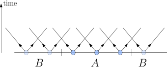
Figure 17: Illustration of the quasiparticle picture for the entanglement spreading in a one-dimensional integrable system. The arrows indicate the propagation of the quasiparticles with the largest velocity $v_{M}$.

In the presence of different species of independent quasiparticles the result can be generalised by summing over them [32],

$$S_{1}(t)=\sum_{m}\left[2t\int_{2v_{m}(k)t<\ell}\mathrm{d}k\ v_{m}(k)s_{m}(k)+\ell\int_{2v_{m}(k)t>\ell}\mathrm{d}k\ s_{m}(k)\right].$$ (6.2)

By properly characterising the functions $v_{m}(k)$ and $s_{m}(k)$, Eq. (6.2) can be applied to all integrable systems [32, 33, 34]. For what follows, it is important to stress that while the generalisation to the Rényi entropies is very easy for free models (in Eq. (6.1) it is enough to replace $s(k)$ with an appropriate $s_{n}(k)$, see [96] and below), it is still an open problem for interacting integrable models [96, 97, 98, 99, 100].

The quasiparticle description can be used to derive analytical predictions for free fermions [32]. The main idea of Ref. [32] is that the kernel $s(k)$ in Eq. (6.1) can be read off from the limit $t\to\infty$, where the density of entanglement entropy equals the density of the thermodynamic entropy in the stationary state, leading to

$$s(k)=\frac{1}{2\pi}(-n_{k}\log n_{k}-(1-n_{k})\log(1-n_{k}))$$ (6.3)

and so

$$S_{1}=\int\frac{\mathrm{d}k}{2\pi}(-n_{k}\log n_{k}-(1-n_{k})\log(1-n_{k}))\min(\ell,2v_{k}t).$$ (6.4)

Here $n_{k}$ is the probability of occupation of the mode $k$ in the steady state. For simplicity, we recast the sum of the two integrals as the integral where the function $\min(\ell,2v_{k}t)$ is included in the integrand. As anticipated, for free models, Eq. (6.1) also holds for the Rényi entropy with the replacement [96]

$$s(k)\to s_{n}(k)=\frac{1}{2\pi}\frac{1}{1-n}\log[n_{k}^{n}+(1-n_{k})^{n}]\,.$$ (6.5)

At this point, it is very natural to generalise the quasiparticle result to charged moments with the natural conjecture

$$\log Z_{n}(\alpha)=\mathrm{i}\alpha\langle Q_{A}\rangle+\int\frac{\mathrm{d}k}{2\pi}\log[n_{k}^{n}\mathsf{e}^{\mathrm{i}\alpha}+(1-n_{k})^{n}]\min(\ell,2v_{k}t).$$ (6.6)

This conjecture matches the exact results for the two quenches considered here where $n_{k}=1/2$ (Néel case) and $n_{k}=(1+\cos k)/2$ (dimer case).

Actually, within free fermion models, the validity of the quasiparticle result (6.6) can be inferred from the following argument. For the Rényi entropy, the quasiparticles conjecture is

$$S_{n}(t)=\frac{1}{1-n}\int\frac{\mathrm{d}k}{2\pi}h_{n,0}(x_{k})\min(\ell,2v_{k}t)=\frac{1}{1-n}\sum_{j=0}^{\infty}c_{n,0}(2j)\int\frac{\mathrm{d}k}{2\pi}x_{k}^{2j}\min(\ell,2v_{k}t),$$ (6.7)

where $x_{k}$ is related to the probability of occupation of the mode $k$ by $n_{k}=(1+x_{k})/2$ and $h_{n,0}(x)$ is given in Eq. (3.6) and has been expanded in $x$ (as in the rightmost side of Eq. (3.6)). In terms of the function $s_{n}(k)$, it is just $h_{n,0}(2n_{k}-1)=2\pi(1-n)s_{n}(k)$. Similarly, the starting formula for the Rényi entropy in terms of the correlation matrix can be expanded as

$$S_{n}(t)=\frac{1}{1-n}\sum_{i=1}^{\ell}\log\left[\left(\frac{1+\nu_{i}}{2}\right)^{n}+\left(\frac{1-\nu_{i}}{2}\right)^{n}\right]=\frac{1}{1-n}\sum_{j=0}^{\infty}c_{n,0}(2j)\text{Tr}J(t)^{2j}.$$ (6.8)

Matching Eqs. (6.8) and (6.7) and properly keeping track of the normalisations (i.e. $\sum_{j=0}^{\infty}c_{n,0}(2j)=h_{n,0}(1)=0$ and $\text{Tr}J(t)^{0}=\ell$), we get

$$\text{Tr}J(t)^{2j}=\ell+\int\frac{\mathrm{d}k}{2\pi}(x_{k}^{2j}-1)\min(\ell,2v_{k}t).$$ (6.9)

Plugging Eq. (6.9) in Eq. (3.7), we obtain the desired result (6.6). As for the total entropies, we conjecture that in the presence of different species of quasiparticles, the result of Eq. (6.6) generalises to a sum over the different species.

6.2 Dynamics of the mutual information

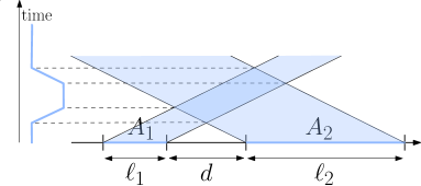
Figure 18: Illustration of the entanglement and mutual information dynamics of two disjoint subsystems. On the left we report the shape of the mutual information with a single velocity of quasiparticles. In the main plot, the dark blue area counts the quasiparticles shared between the two disjoint sets.

Let us consider the case in which the subsystem $A$ of length $\ell$ is formed by two disjoint intervals $A_{1}$ and $A_{2}$ of respective lengths $\ell_{1}$ and $\ell_{2}$ that are separated by a distance $d$. Without loss of generality we consider $\ell_{1}\leqslant\ell_{2}$. Since the total mutual information is a combination of entanglement entropies for which the quasiparticle picture holds, it is natural that it must be related to the number of entangled pairs that, once emitted from the same point, are shared by the two subsystem at subsequent times.

This counting of quasiparticles is straightforward, but we report it here for completeness. Let us first assume that the quasiparticles possess a single velocity $v$. It follows that for short times $t\leqslant d/(2v)$ there are no entangled quasiparticles shared by the two intervals and the mutual information is zero. It then increases linearly for $d/(2v)\leqslant t\leqslant(d+\ell_{1})/(2v)$. There is a plateau for $(d+\ell_{1})/(2v)\leqslant t\leqslant(d+\ell_{2})/(2v)$, after which it decreases linearly in time up to $t=(d+\ell)/2v$. There are no longer any quasiparticles shared between the subsystems for larger times, so that the mutual information vanishes for $t\geqslant(d+\ell)/2v$. We illustrate this behaviour in Fig. 18. Accordingly, the resulting dynamics of the mutual information is proportional to $[\max(d,2vt)+\max(d+\ell,2vt)-\max(d+\ell_{1},2vt)-\max(d+\ell_{2},2vt)]$[21, 24].

In the presence of a non-trivial dispersion (and hence different velocities $v(k)$), it is enough to integrate over $k$ to get [32, 33]

$$I_{1}^{A_{1}:A_{2}}=\int\mathrm{d}k\ s(k)[\max(d,2v(k)t)+\max(d+\ell,2v(k)t)-\max(d+\ell_{1},2v(k)t)-\max(d+\ell_{2},2v(k)t)],$$ (6.10)

with $s(k)$ in Eq. (6.3) for free fermions.

For the charged moment $\log Z_{n}^{A_{1}\cup A_{2}}(\alpha)$ it is straightforward to adapt the argument of the previous subsection to get

$$\log Z_{n}^{A_{1}\cup A_{2}}(\alpha)=\mathrm{i}\alpha\langle Q_{A}\rangle+\int\frac{\mathrm{d}k}{2\pi}\mathrm{Re}[h_{n,\alpha}(x_{k})][\min(\ell_{1},2v_{k}t)+\min(\ell_{2},2v_{k}t)]\\ -\int\frac{\mathrm{d}k}{2\pi}\mathrm{Re}[h_{n,\alpha}(x_{k})][\max(d,2v_{k}t)+\max(d+\ell,2v_{k}t)-\max(d+\ell_{1},2v_{k}t)-\max(d+\ell_{2},2v_{k}t)].$$ (6.11)

This equation precisely matches our analytical results from Eqs. (4.33) with $x_{k}=0$ for the quench from the Néel state, and (5.23) with $x_{k}=\cos k$ in the case of the quench from the dimer state.

To determine the symmetry resolved mutual information, we also need the moment $Z_{1}(\alpha,\beta)$ defined in Eq. (2.11). Our results of Eqs. (4.38) and (5.36) suggest the general quasiparticle expression

$$\log Z_{1}^{A_{1}:A_{2}}(\alpha,\beta)=\mathrm{i}\alpha\langle Q_{A_{1}}\rangle+\mathrm{i}\beta\langle Q_{A_{2}}\rangle+\int\frac{\mathrm{d}k}{2\pi}\mathrm{Re}[h_{1,\alpha}(x_{k})]\min(\ell_{1},2v_{k}t)+\int\frac{\mathrm{d}k}{2\pi}\mathrm{Re}[h_{1,\beta}(x_{k})]\min(\ell_{2},2v_{k}t)\\ -\frac{1}{2}\int\frac{\mathrm{d}k}{2\pi}\mathrm{Re}[h_{1,\alpha}(x_{k})+h_{1,\beta}(x_{k})-h_{1,\alpha-\beta}(x_{k})](\max(d,2v_{k}t)\\ +\max(d+\ell,2v_{k}t)-\max(d+\ell_{1},2v_{k}t)-\max(d+\ell_{2},2v_{k}t)).$$ (6.12)

As in the case of a single interval, we conjecture that in the presence of different species of quasiparticles, the results of Eqs. (6.11) and (6.12) generalise to a sum over the different species.

7 Conclusions

In this manuscript, we study the symmetry resolved entanglement after a quantum quench in the one-dimensional tight binding model. We start from the calculation of the charged moments $Z_{n}(\alpha)$ (cf. Eq. (2.5)) that have been exactly determined by adapting the multidimensional stationary phase calculation of Ref. [87], see [89]. Our results for $Z_{n}(\alpha)$ are also valid when the subsystem $A$ consists of two (or more) disjoint intervals. From the charged moments, the symmetry resolved entropy is obtained by Fourier transform and saddle point approximation in the charge flux. The structure of charged moments leads to two main physical results. First, the symmetry resolved entanglement with charge $\Delta q=q-\langle Q_{A}\rangle$ starts evolving only after a (calculable) delay time proportional to $|\Delta q|$. Second, for small $|\Delta q|$ there is an effective equipartition of entanglement broken at order $\Delta q^{2}/\ell$. We also introduced a symmetry resolved mutual information (2.9) that requires the computation of a charged moment with two independent flux insertions, see Eq. (2.11). We worked out exact predictions for this more complicated charged moment for two quenches in our models. We also found that the number entropy grows logarithmically with time before saturating to a value proportional to the logarithm of the subsystem size.

Our results for free fermions naturally lead to a conjecture based on the quasiparticle picture for $Z_{n}(\alpha)$ that can generically be written as

$$\log Z_{n}(\alpha)=\mathrm{i}\alpha\langle Q_{A}\rangle+\sum_{m}\int\frac{\mathrm{d}k}{2\pi}s_{n,\alpha}^{m}(k)\min(\ell,2v_{m}(k)t)$$ (7.1)

where the sum is over the independent quasiparticles’ species (where the velocities $v_{m}(k)$ also depend on the state [101]). To give predictive power to this conjecture we should still devise a way to fix the kernel $s_{n,\alpha}^{m}(k)$, but how to do this is still not know for an interacting model, as already discussed for the Rényi entropy in Refs. [96, 97, 98, 99, 100]. The solution is known only in the neighbourhood of $n=1$ where the kernel is the Yang-Yang entropy [32]. It would already be interesting to generalise this result at $n=1$ and small $\alpha\neq 0$, that would be enough for the saddle-point approximation necessary to get the symmetry resolution. Independently of the details of the function $s_{n,\alpha}^{m}(k)$, the form of the conjecture (7.1) is sufficient to deduce the two main physical results, i.e. existence of the delay time and equipartition for small $|\Delta q|$ for a generic integrable model. Moreover, the logarithmic growth of the number entropy follows from the behaviour of $Z_{1}(\alpha)$ close to $\alpha=0$ and so follows generically from  Eq. (7.1).

Similarly to the charged moments, we conjectured that the doubly-charged moments $Z_{1}(\alpha,\beta)$ in Eq. (2.11) needed to investigate the symmetry resolved mutual information can be described in the framework of the quasiparticle picture, see Eq. (6.12).

We conclude this manuscript by speculating on some generalisations of our results. A first question is whether symmetry resolved entropies can be obtained in inhomogeneous settings, as done for the total entropy in Refs. [103, 104, 105, 106, 107, 108]. Then, it is natural to wonder if some of the techniques developed for non-integrable models [109, 110, 111, 114, 115, 116, 117, 118, 112, 113, 119] apply to the symmetry resolved quantities and whether our main physical findings, time delay and equipartition, are robust.

References

- [1] A. Polkovnikov, K. Sengupta, A. Silva, and M. Vengalattore, Colloquium: Nonequilibrium dynamics of closed interacting quantum systems, Rev. Mod. Phys. 83, 863 (2011).
- [2] C. Gogolin and J. Eisert, Equilibration, thermalisation, and the emergence of statistical mechanics in closed quantum systems, Rep. Prog. Phys. 79, 056001 (2016).
- [3] L. D’Alessio, Y. Kafri, A. Polkovnikov, and M. Rigol, From Quantum Chaos and Eigenstate Thermalization to Statistical Mechanics and Thermodynamics, Adv. Phys. 65, 239 (2016).
- [4] P. Calabrese, F. H. L. Essler, and G. Mussardo, Introduction to ’Quantum Integrability in Out of Equilibrium Systems’, J. Stat. Mech. (2016) 064001.
- [5] F. H. L. Essler and M. Fagotti, Quench dynamics and relaxation in isolated integrable quantum spin chains, J. Stat. Mech. (2016) 064002.
- [6] P. Calabrese, Entanglement and thermodynamics in non-equilibrium isolated quantum systems, Physica A 504, 31 (2018).
- [7] J. M. Deutsch, H. Li, and A. Sharma, Microscopic origin of thermodynamic entropy in isolated systems, Phys. Rev. E 87, 042135 (2013).
- [8] L. F. Santos, A. Polkovnikov, and M. Rigol, Entropy of Isolated Quantum Systems after a Quench, Phys. Rev. Lett. 107, 040601 (2011).
- [9] M. Collura, M. Kormos, and P. Calabrese, Stationary entanglement entropies following an interaction quench in Bose gas, J. Stat. Mech. (2014) P01009.
- [10] N. Schuch, M. M. Wolf, F. Verstraete, and J. I. Cirac, Entropy Scaling and Simulability by Matrix Product States, Phys. Rev. Lett. 100, 030504 (2008).
- [11] N. Schuch, M. M. Wolf, K. G. H. Vollbrecht, and J. I. Cirac, On entropy growth and the hardness of simulating time evolution, New J. Phys. 10, 033032 (2008).
- [12] A. Perales and G. Vidal, Entanglement growth and simulation efficiency in one-dimensional quantum lattice systems, Phys. Rev. A 78, 042337 (2008).
- [13] P. Hauke, F. M. Cucchietti, L. Tagliacozzo, I. Deutsch, and M. Lewenstein, Can one trust quantum simulators? Prog. Phys. 75 082401 (2012).
- [14] J. Dubail, Entanglement scaling of operators: a conformal field theory approach, with a glimpse of simulability of long-time dynamics in 1+1d, J. Phys. A 50, 234001 (2017).
- [15] P. Calabrese and J. Cardy, Entanglement entropy and quantum field theory, J. Stat. Mech. (2004) P06002
- [16] P. Calabrese and A. Lefevre, Entanglement spectrum in one-dimensional systems, Phys. Rev. A 78, 032329 (2008)
- [17] M. M. Wolf, F. Verstraete, M.B. Hastings, and I. J. Cirac, Area Laws in Quantum Systems: Mutual Information and Correlations, Phys. Rev. Lett. 100, 070502 (2008).
- [18] M. Kormos and Z. Zimboras, Temperature driven quenches in the Ising model: appearance of negative Rényi mutual information, J. Phys. A 50, 264005 (2017).
- [19] S. O. Scalet, A. M. Alhambra, G. Styliaris, and J. I. Cirac, Computable Rényi mutual information: Area laws and correlations, arXiv:2103.01709.
- [20] G. Vidal and R. F. Werner, Computable measure of entanglement, Phys. Rev. A 65, 032314 (2002).
- [21] A. Coser, E. Tonni, and P. Calabrese, Entanglement negativity after a global quantum quench, J. Stat. Mech. (2014) P12017.
- [22] V. Eisler and Z. Zimborás, Entanglement negativity in the harmonic chain out of equilibrium, New J. Phys. 16, 123020 (2014).
- [23] M. Hoogeveen and B. Doyon, Entanglement negativity and entropy in non-equilibrium conformal field theory, Nucl. Phys. B 898, 78 (2015).
- [24] V. Alba and P. Calabrese, Quantum information dynamics in multipartite integrable systems, EPL 126, 60001 (2019).
- [25] M. J. Gullans and D. A. Huse, Entanglement Structure of Current-Driven Diffusive Fermion Systems, Phys. Rev. X 9, 021007 (2019).
- [26] J. Kudler-Flam, Y. Kusuki, and S. Ryu, The quasi-particle picture and its breakdown after local quenches: mutual information, negativity, and reflected entropy, JHEP 03 (2021) 146.
- [27] E. Wybo, M. Knap, and F. Pollmann, Entanglement dynamics of a many-body localized system coupled to a bath, Phys. Rev. B 102, 064304 (2020).
- [28] G. Parez, R. Bonsignori, P. Calabrese, Dynamics of charge-imbalance-resolved entanglement negativity after a quench in a free-fermion model, J. Stat. Mech. (2022) 053103.
- [29] P. Calabrese and J. Cardy, Time-dependence of correlation functions following a quantum quench, Phys. Rev. Lett. 96 136801 (2006).
- [30] P. Calabrese and J. Cardy, Quantum Quenches in Extended Systems, J. Stat. Mech. (2007) P06008.
- [31] P. Calabrese and J. Cardy, Evolution of Entanglement Entropy in One-Dimensional Systems, J. Stat. Mech. (2005) P04010.
- [32] V. Alba and P. Calabrese, Entanglement and thermodynamics after a quantum quench in integrable systems, PNAS 114, 7947 (2017).
- [33] V. Alba and P. Calabrese, Entanglement dynamics after quantum quenches in generic integrable systems, SciPost Phys. 4, 017 (2018).
- [34] P. Calabrese, Entanglement spreading in non-equilibrium integrable systems, Lectures for Les Houches Summer School on “Integrability in Atomic and Condensed Matter Physics”, SciPost Phys. Lect. Notes 20 (2020).
- [35] A. M. Kaufman, M. E. Tai, A. Lukin, M. Rispoli, R. Schittko, P. M. Preiss, and M. Greiner, Quantum thermalisation through entanglement in an isolated many-body system, Science 353, 794 (2016).
- [36] A. Lukin, M. Rispoli, R. Schittko, M. E. Tai, A. M. Kaufman, S. Choi, V. Khemani, J. Leonard, and M. Greiner, Probing entanglement in a many-body localized system, Science 364, 6437 (2019).
- [37] T. Brydges, A. Elben, P. Jurcevic, B. Vermersch, C. Maier, B. P. Lanyon, P. Zoller, R. Blatt, and C. F. Roos, Probing Rényi entanglement entropy via randomized measurements, Science 364, 260 (2019).
- [38] A. Elben, R. Kueng, H.-Y. Huang, R. van Bijnen, C. Kokail, M. Dalmonte, P. Calabrese, B. Kraus, J. Preskill, P. Zoller, and B. Vermersch, Mixed-state entanglement from local randomized measurements, Phys. Rev. Lett. 125, 200501 (2020).
- [39] M. Goldstein and E. Sela, Symmetry Resolved Entanglement in Many-Body Systems, Phys. Rev. Lett. 120, 200602 (2018).
- [40] J. C. Xavier, F. C. Alcaraz, and G. Sierra, Equipartition of the entanglement entropy, Phys. Rev. B 98, 041106 (2018).
- [41] E. Cornfeld, M. Goldstein, and E. Sela, Imbalance Entanglement: Symmetry Decomposition of Negativity, Phys. Rev. A 98, 032302 (2018).
- [42] R. Bonsignori, P. Ruggiero, and P. Calabrese, Symmetry resolved entanglement in free fermionic systems, J. Phys. A: Math. Theor. 52, 475302 (2019).
- [43] R. Bonsignori and P. Calabrese, Boundary effects on symmetry resolved entanglement, J. Phys. A: Math. Theor. 54, 015005 (2020).
- [44] S. Fraenkel and M. Goldstein, Symmetry resolved entanglement: Exact results in 1d and beyond, J. Stat. Mech. (2020) 033106.
- [45] G. Parez, R. Bonsignori and P. Calabrese, Quasiparticle dynamics of symmetry-resolved entanglement after a quench: Examples of conformal field theories and free fermions Phys. Rev. B 103, L041104 (2021).
- [46] N. Feldman and M. Goldstein, Dynamics of Charge-Resolved Entanglement after a Local Quench, Phys. Rev. B 100, 235146 (2019).
- [47] P. Caputa, G. Mandal, and R. Sinha, Dynamical entanglement entropy with angular momentum and U(1) charge, J. High Energ. Phys. 2013, 52 (2013)
- [48] P. Caputa, M. Nozaki, and T. Numasawa, Charged entanglement entropy of local operators, Phys. Rev. D 93, 105032 (2016)
- [49] L. Capizzi, P. Ruggiero, and P. Calabrese, Symmetry resolved entanglement entropy of excited states in a CFT , J. Stat. Mech. (2020) 073101.
- [50] N. Laflorencie and S. Rachel, Spin-resolved entanglement spectroscopy of critical spin chains and Luttinger liquids, J. Stat. Mech. (2014) P11013.
- [51] S. Murciano, G. Di Giulio, and P. Calabrese, Entanglement and symmetry resolution in two dimensional free quantum field theories, JHEP 08 (2020) 073.
- [52] S. Murciano, G. Di Giulio, and P. Calabrese, Symmetry resolved entanglement in gapped integrable systems: a corner transfer matrix approach, SciPost Phys. 8, 046 (2020).
- [53] P. Calabrese, M. Collura, G. Di Giulio, and S. Murciano, Full counting statistics in the gapped XXZ spin chain, EPL 129, 60007 (2020).
- [54] S. Murciano, R. Bonsignori, P. Calabrese, Symmetry decomposition of negativity of massless free fermions, SciPost Phys. 10, 111 (2021)
- [55] M. T. Tan and S. Ryu, Particle number fluctuations, Rényi and symmetry-resolved entanglement entropy in two-dimensional Fermi gas from multi-dimensional bosonisation, Phys. Rev. B 101, 235169 (2020).
- [56] S. Murciano, P. Ruggiero, and P. Calabrese, Symmetry resolved entanglement in two-dimensional systems via dimensional reduction, J. Stat. Mech. (2020) 083102.
- [57] X. Turkeshi, P. Ruggiero, V. Alba, and P. Calabrese, Entanglement equipartition in critical random spin chains, Phys. Rev. B 102, 014455 (2020).
- [58] K. Monkman and J. Sirker, Operational Entanglement of Symmetry-Protected Topological Edge States, Phys. Rev. Res. 2, 043191 (2020).
- [59] E. Cornfeld, L. A. Landau, K. Shtengel, and E. Sela, Entanglement spectroscopy of non-Abelian anyons: Reading off quantum dimensions of individual anyons, Phys. Rev. B 99, 115429 (2019).
- [60] D. X. Horváth and P. Calabrese, Symmetry resolved entanglement in integrable field theories via form factor bootstrap, JHEP 11 (2020) 131.
- [61] D. X. Horvath, L. Capizzi, and P. Calabrese, U(1) symmetry resolved entanglement in free 1+1 dimensional field theories via form factor bootstrap, arXiv:2103.03197.
- [62] D. Azses and E. Sela, Symmetry-resolved entanglement in symmetry-protected topological phases, Phys. Rev. B 102, 235157 (2020).
- [63] V. Vitale, A. Elben, R. Kueng, A. Neven, J. Carrasco, B. Kraus, P. Zoller, P. Calabrese, B. Vermersch, and M. Dalmonte, Symmetry-resolved dynamical purification in synthetic quantum matter, arXiv:2101.07814.
- [64] S. Fraenkel and M. Goldstein, Entanglement Measures in a Nonequilibrium Steady State: Exact Results in One Dimension, arXiv:2105.00740.
- [65] A. Neven, J. Carrasco, V. Vitale, C. Kokail, A. Elben, M. Dalmonte, P. Calabrese, P. Zoller, B. Vermersch, R. Kueng, and B. Kraus, Symmetry-resolved entanglement detection using partial transpose moments, arXiv:2103.07443
- [66] B. Estienne, Y. Ikhlef and A. Morin-Duchesne, Finite-size corrections in critical symmetry-resolved entanglement, SciPost Phys. 10, 54 (2021).
- [67] H.-H. Chen, Symmetry decomposition of relative entropies in conformal field theory, arXiv:2104.03102.
- [68] L. Capizzi and P. Calabrese, Symmetry resolved relative entropies and distances in conformal field theory, arXiv:2105.08596.
- [69] D. X. Horvath, P. Calabrese, and O. A. Castro-Alvaredo, Branch Point Twist Field Form Factors in the sine-Gordon Model II: Composite Twist Fields and Symmetry Resolved Entanglement, arXiv:2105.13982.
- [70] S. Zhao, C. Northe, and R. Meyer Symmetry-Resolved Entanglement in AdS3/CFT2 coupled to Chern-Simons Theory, arXiv:2012.11274
- [71] H. M. Wiseman and J. A. Vaccaro, Entanglement of Indistinguishable Particles Shared between Two Parties, Phys. Rev. Lett. 91, 097902 (2003).
-
[72]
H. Barghathi, C. M. Herdman, and A. Del Maestro, Rényi Generalization of the Accessible Entanglement Entropy,
Phys. Rev. Lett. 121, 150501 (2018);
H. Barghathi, E. Casiano-Diaz, and A. Del Maestro, Operationally accessible entanglement of one dimensional spinless fermions, Phys. Rev. A 100, 022324 (2019). - [73] M. Kiefer-Emmanouilidis, R. Unanyan, J. Sirker, and M. Fleischhauer, Bounds on the entanglement entropy by the number entropy in non-interacting fermionic systems, SciPost Phys. 8, 083 (2020).
- [74] M. Kiefer-Emmanouilidis, R. Unanyan, J. Sirker, and M. Fleischhauer, Evidence for unbounded growth of the number entropy in many-body localized phases, Phys. Rev. Lett. 124, 243601 (2020).
- [75] M. Kiefer-Emmanouilidis, R. Unanyan, M. Fleischhauer, and J. Sirker, Slow delocalization of particles in many-body localized phases, Phys. Rev. B 103, 024203 (2021).
- [76] Y. Zhao, D. Feng, Y. Hu, S. Guo, and J. Sirker, Entanglement dynamics in the three-dimensional Anderson model, Phys. Rev. B 102, 195132 (2020).
- [77] M. Kiefer-Emmanouilidis, R. Unanyan, M. Fleischhauer, and J. Sirker, Unlimited growth of particle fluctuations in many-body localized phases, Ann. Phys. 168481 (2021).
- [78] X. Cao, A. Tilloy, and A. De Luca, Entanglement in a fermion chain under continuous monitoring, SciPost Phys. 7, 024 (2019).
- [79] M. C. Chung and I. Peschel, Density-matrix spectra of solvable fermionic systems, Phys. Rev. B 64, 064412 (2001).
- [80] I. Peschel, Calculation of reduced density matrices from correlation functions, J. Phys. A 36, L205 (2003).
- [81] I. Peschel and V. Eisler, Reduced density matrices and entanglement entropy in free lattice models, J. Phys. A 42, 504003 (2009).
- [82] V. Alba, L. Tagliacozzo, and P. Calabrese, Entanglement entropy of two disjoint blocks in critical Ising models, Phys. Rev. B 81, 060411 (2010).
- [83] F. Igloi and I. Peschel, On reduced density matrices for disjoint subsystems, EPL 89, 40001 (2010).
- [84] M. Fagotti and P. Calabrese, Entanglement entropy of two disjoint blocks in XY chains, J. Stat. Mech. (2010) P04016.
- [85] S. Groha, F. Essler, and P.Calabrese, Full counting statistics in the transverse field Ising chain, SciPost Phys. 4, 043 (2018).
- [86] R. Balian and E. Brezin, Nonunitary Bogoliubov transformations and extension of Wick’s theorem, Il Nuovo Cimento B 64, 37 (1969).
- [87] M. Fagotti and P. Calabrese, Evolution of entanglement entropy following a quantum quench: Analytic results for the XY chain in a transverse magnetic field, Phys. Rev. A 78, 010306(R).
- [88] Eq. (4.9) is an integral representation of the reciprocal function, see Wikipedia. Alternatively, see Eq. 3.631-9 in Gradshteyn and Ryzhik’s, Table of Integrals, Series, and Products, 5th edition, Academic Press.
- [89] G. Parez and R. Bonsignori, Analytical results for the entanglement dynamics of disjoint blocks in the XY spin chain, arXiv:2210.03637.
- [90] M. Fagotti, On conservation laws, relaxation and pre-relaxation after a quantum quench, J. Stat. Mech. (2014) P03016.
- [91] B. Bertini, E. Tartaglia, and P. Calabrese, Entanglement and diagonal entropies after a quench with no pair structure, J. Stat. Mech. (2018) 063104.
- [92] A. Bastianello and P. Calabrese, Spreading of entanglement and correlations after a quench with intertwined quasiparticles, SciPost Phys. 5, 033 (2018).
- [93] A. Bastianello and M. Collura, Entanglement spreading and quasiparticle picture beyond the pair structure, SciPost Phys. 8, 045 (2020).
- [94] L. Piroli, B. Pozsgay, and E. Vernier, What is an integrable quench?, Nucl. Phys. B 925, 362 (2017).
- [95] E.H. Lieb and D. W. Robinson, The finite group velocity of quantum spin systems, Commun. Math. Phys. 28, 251 (1972).
- [96] V. Alba and P. Calabrese, Quench action and Rényi entropies in integrable systems, Phys. Rev. B 96, 115421 (2017).
- [97] V. Alba and P. Calabrese, Rényi entropies after releasing the Néel state in the XXZ spin-chain, J. Stat. Mech. (2017) 113105.
- [98] M. Mestyán, V. Alba, and P. Calabrese, Rényi entropies of generic thermodynamic macrostates in integrable systems, J. Stat. Mech. (2018) 083104.
- [99] O. A. Castro-Alvaredo, M. Lencses, I. M. Szecsenyi and J. Viti, Entanglement dynamics after a quench in Ising field theory: a branch point twist field approach, JHEP 12 (2019) 079.
- [100] K. Klobas and B. Bertini, Entanglement dynamics in Rule 54: exact results and quasiparticle picture, arXiv:2104.04513
- [101] L. Bonnes, F.H.L. Essler, and A. M. Läuchli, Light-cone dynamics after quantum quenches in spin chains, Phys. Rev. Lett. 113, 187203 (2014).
- [102] G. Perfetto, L. Piroli, and A. Gambassi, Quench action and large deviations: Work statistics in the one-dimensional Bose gas, Phys. Rev. E 100, 032114 (2019).
- [103] V. Alba, Entanglement and quantum transport in integrable systems, Phys. Rev. B 97, 245135 (2018).
- [104] B. Bertini, M. Fagotti, L. Piroli, and P. Calabrese, Entanglement evolution and generalised hydrodynamics: noninteracting systems, J. Phys. A 51, 39LT01 (2018).
- [105] V. Alba, B. Bertini, and M. Fagotti, Entanglement evolution and generalised hydrodynamics: interacting integrable systems, SciPost Phys. 7, 005 (2019).
- [106] V. Alba, Towards a generalized hydrodynamics description of Rényi entropies in integrable systems, Phys. Rev. B 99, 045150 (2019).
- [107] J. Dubail, J.-M. Stéphan, J. Viti, and P. Calabrese, Conformal field theory for inhomogeneous one-dimensional quantum systems: the example of non-interacting Fermi gases, SciPost Phys. 2, 002 (2017).
- [108] P. Ruggiero, P. Calabrese, B. Doyon, and J. Dubail, Quantum Generalized Hydrodynamics, Phys. Rev. Lett. 124, 140603 (2020)
- [109] A. Nahum, J. Ruhman, S. Vijay, and J. Haah, Quantum Entanglement Growth under Random Unitary Dynamics, Phys. Rev. X 7, 031016 (2017).
- [110] A. Nahum, S. Vijay, and J. Haah, Operator Spreading in Random Unitary Circuits, Phys. Rev. X 8, 021014 (2018).
- [111] T. Zhou and A. Nahum, The entanglement membrane in chaotic many-body systems, Phys. Rev. X 10, 031066 (2020).
- [112] A. Chan, A. De Luca, and J. T. Chalker, Solution of a minimal model for many-body quantum chaos, Phys. Rev. X 8, 041019 (2018).
- [113] A. J. Friedman, A. Chan, A. De Luca, and J. T. Chalker, Spectral statistics and many-body quantum chaos with conserved charge, Phys. Rev. Lett. 123, 210603 (2019).
- [114] B. Bertini, P. Kos, and T. Prosen, Entanglement Spreading in a Minimal Model of Maximal Many-Body Quantum Chaos, Phys. Rev. X 9, 021033 (2019).
- [115] S. Gopalakrishnan and A. Lamacraft, Unitary circuits of finite depth and infinite width from quantum channels, Phys. Rev. B 100, 064309 (2019).
- [116] B. Bertini and P. Calabrese, Prethermalisation and Thermalisation in the Entanglement Dynamics, Phys. Rev. B 102, 094303 (2020).
- [117] L. Piroli, B. Bertini, J. I. Cirac, and T. Prosen, Exact dynamics in dual-unitary quantum circuits, Phys. Rev. B 101, 094304 (2020).
- [118] R. Modak, V. Alba, and P. Calabrese, Entanglement revivals as a probe of scrambling in finite quantum systems, J. Stat. Mech. (2020) 083110.
- [119] T. Rakovszky, F. Pollmann, and C. W. von Keyserlingk, Sub-ballistic Growth of Rényi Entropies due to Diffusion, Phys. Rev. Lett. 122, 250602 (2019).