Angular momentum distribution in a relativistic configuration: Magnetic quantum number analysis

Abstract

This paper is devoted to the analysis of the distribution of the total magnetic quantum number $M$ in a relativistic subshell with $N$ equivalent electrons of momentum $j$. This distribution is analyzed through its cumulants and through their generating function, for which an analytical expression is provided. This function also allows us to get the values of the cumulants at any order. Such values are useful to obtain the moments at various orders. Since the cumulants of the distinct subshells are additive this study directly applies to any relativistic configuration. Recursion relations on the generating function are given. It is shown that the generating function of the magnetic quantum number distribution may be expressed as a n-th derivative of a polynomial. This leads to recurrence relations for this distribution which are very efficient even in the case of large $j$ or $N$. The magnetic quantum number distribution is numerically studied using the Gram-Charlier and Edgeworth expansions. The inclusion of high-order terms may improve the accuracy of the Gram-Charlier representation for instance when a small and a large angular momenta coexist in the same configuration. However such series does not exhibit convergence when high orders are considered and the account for the first two terms often provides a fair approximation of the magnetic quantum number distribution. The Edgeworth series offers an interesting alternative though this expansion is also divergent and of asymptotic nature.

I Introduction

The theoretical study of emission or absorption spectral properties of hot plasmas, encountered for instance in stellar physics, inertial-confinement fusion, or laser-plasma experiments, implies taking into account complex ions, i.e., multi-electron configurations with several open subshells. The issue of finding the number of states corresponding to a given $(J,M)$ set — $J$ being the magnitude of the total angular momentum operator and $M$ the eigenvalue (in units of $\hbar$) of its projection on the $z$-axis — in the case of a set of indistinguishable particles was first investigated by Bethe in 1936 for nuclear systems [1]. The problem of the classification of atomic energy levels is discussed in many textbooks about quantum mechanics. The determination of the spectroscopic terms arising in a given electronic configuration was addressed by different methods, the first one being the so-called vector model [2]. The properties (regularities, trends) of such terms were also investigated [3]. The problem of listing the terms arising in a complex configuration can be solved from elementary group theory [4, 5, 6, 7, 8]. Besides, the determination of the number of lines between two configurations is of great interest. Using group-theoretical methods, Krasnitz obtained a compact formula only in the simple case of configurations built with non-equivalent electrons [9]. The statistics of electric-dipole (E1) lines was studied by Moszkowski [10], Bancewicz [11], Bauche and Bauche-Arnoult [12, 13], and more recently by Gilleron and Pain [14]. Such a quantity is important for opacity codes, for instance, in order to decide whether a transition array can be described statistically or requires a detailed-line accounting calculation, relying on the diagonalization of the Hamiltonian [15]. In the same spirit, the statistics of electric quadrupole (E2) lines was also investigated [16]. A particular case of fluctuation, the odd-even staggering (i.e., the fact that, in an electronic configuration, the number of odd values of $J$ can differ from the number of even values of $J$), was studied by Bauche and Cossé [17] and later revisited using the generating-function technique [18].

Except maybe for the odd-even staggering, the knowledge of the moments or cumulants can be very useful to build a statistical modeling. This was carried out by Bauche et al. [12] for the distributions of energy levels and spectroscopic terms in an electronic configuration or for the distribution of absorption or emission lines. For instance, following the pioneering work of Moszkowski [19], the first two moments of the line energies weighted by their strengths in a transition array were calculated exactly by Bauche et al. [9]. The work on averages of products of operators by Ginocchio [20] enabled Kučas and Karazija [21, 22] to find an algorithm to generate the moment of any order and the impact of higher-order moments (without calculating them explicitly) was studied recently by Gilleron and Pain [23]. Kyniėne et al. investigated the statistical properties of Auger transitions and obtained a fair approximation for the number of Auger amplitudes [24]. The authors showed that statistical properties of Auger spectra mainly depend on the orbital quantum numbers of shells involved in the transitions and that rather large values of skewness and excess kurtosis indicate a significant deviation of the distribution of Auger amplitudes from the normal distribution. Moreover, the generating-function formalism is a powerful tool for tackling the counting problems, either for finding analytical expressions, deriving recursion relations or performing a statistical analysis. Using such a formalism, we recently published explicit and recurrence formulas for the number of electronic configurations in an atom [25], together with a statistical analysis through the computation of cumulants.

The object of this work is to show that similar considerations apply to the distribution of the magnetic quantum number in a relativistic configuration. The present paper is organized as follows. General formulas for the magnetic quantum number distribution $P(M)$ are recalled in section II. The generating function of cumulants of this distribution in a single- or multiple-subshell configuration is derived in the same section. In section III, recurrence relations are deduced from the expression of the quantum number distribution as a n-th derivative. The analytical expression of the cumulants is obtained in section IV and an additional recurrence relation for their generating function is provided in section V. An analysis of the distribution using Gram-Charlier and Edgeworth series is carried out in sections VI and VII respectively, and the paper ends with instructive general considerations about the distribution $P(M)$.

II Characterization of the magnetic quantum number distribution: the cumulant generating function

II.1 Definitions

Our main objective is to determine the statistics of the angular quantum number $J$. However, due to the fact that the quantum number $J$ is the eigenvalue of no simple operator, its mathematical study is tedious. Therefore, it is more appropriate to study the distribution of the magnetic quantum number $M$, another advantage being that when different subshells are present their contributions to $M$ simply add up. The $J$ values can be obtained from the $M$ values by means of the method of Condon and Shortley [26], which enables one to express the number $Q(J)$ of levels with angular momentum $J$ in a configuration as

$$Q(J)=\sum_{M=J}^{J+1}(-1)^{J-M}P\left(M\right)=P\left(M=J\right)-P\left(M=J+1\right),$$ (II.1)

where $P$ represents the distribution of the angular-momentum projection $M$. In this work, we consider the case of relativistic configurations, which means that individual electrons are labeled by their total angular momentum $j$. Pauli principle is fully accounted for. For a configuration $j_{1}^{N_{1}}j_{2}^{N_{2}}j_{3}^{N_{3}}\cdots j_{w}^{N_{w}}$, $P(M)$ is determined through the relation

$$P_{N_{1},N_{2},\cdots}\left(M\right)=\left(P_{N_{1}}\otimes P_{N_{2}}\otimes P_{N_{3}}\otimes\cdots\otimes P_{N_{w}}\right)\left(M\right),$$ (II.2)

where the distributions are convolved two at a time, which means that

$$\left(P_{N_{i}}\otimes P_{N_{j}}\right)\left(M\right)=\sum_{M^{\prime}=-\infty}^{\infty}P_{N_{i}}\left(M^{\prime}\right)P_{N_{j}}\left(M-M^{\prime}\right).$$ (II.3)

Let us consider a system of $N$ identical fermions in a configuration consisting of a single orbital of degeneracy $g$, $m_{i}$ being the angular momentum projection of electron state $i$. Two constraints must be satisfied:

$$N=n_{1}+\cdots+n_{g}=\sum_{i=1}^{g}n_{i},$$ (II.4)

where $n_{i}$ is the number of electrons in state $i$ and

$$M=n_{1}m_{1}+\cdots+n_{g}m_{g}=\sum_{i=1}^{g}n_{i}m_{i},$$ (II.5)

where $n_{i}=0$ or 1 $\forall i$. In the particular case of the relativistic configuration $j^{N}$, the maximum total angular momentum is

$$J_{\text{max}}=\sum_{m=j-N+1}^{j}m=(2j+1-N)N/2.$$ (II.6)

As stated in statistical treatises [27], the whole information about the distribution $P(M)$ of magnetic quantum number is contained in the exponential of the cumulant generating function defined as

$$\exp(K(t))=\left<\exp(tM)\right>=\sum_{M}P(M)e^{tM}\left/\sum_{M}P(M)\right.$$ (II.7)

where $P(M)$ is the number of $N$-electron states such as $m_{1}+\cdots m_{N}=M$. From the Pauli principle this normalization factor is given by the product of simple binomial coefficients

$$\sum_{M}P(M)=\prod_{s=1}^{w}\binom{2j_{s}+1}{N_{s}}.$$ (II.8)

II.2 Derivation from a recurrence relation in a single-subshell case

As a first step we consider relativistic configurations containing only one subshell symbolically written $j^{N}$. One may express the population $P(M)$ as a multiple-sum over each magnetic level population [14]

$$P(M)=\sum_{p_{1}=0}^{1}\sum_{p_{2}=0}^{1}\cdots\sum_{p_{g}=0}^{1}\delta\left(M-\sum_{k=1}^{g}p_{k}m_{k}\right)\ \delta\left(N-\sum_{k=1}^{g}p_{k}\right)$$ (II.9)

where $p_{k}$ is the $k$-state population and $g=2j+1$ the subshell degeneracy. The Kronecker symbol $\delta_{i,j}$ is written here $\delta(i-j)$ for the sake of readability. Each $p_{k}$ is either 0 or 1, and the individual magnetic quantum numbers are

$$m_{1}=-j,m_{2}=-j+1,\cdots m_{g}=j.$$ (II.10)

Writing the numerator in (II.7) as

$$s(N,j,t)=\sum_{M}P(M)e^{Mt}$$ (II.11)

one has

$$s(N,j,t)=\sum_{M}\sum_{p_{1}=0}^{1}\sum_{p_{2}=0}^{1}\cdots\sum_{p_{g}=0}^{1}\delta\left(M-\sum_{k=1}^{g}p_{k}m_{k}\right)\ \delta\left(N-\sum_{k=1}^{g}p_{k}\right)e^{Mt}$$ (II.12)

in which the sum over $M$ may be eliminated

$$s(N,j,t)=\sum_{p_{1}=0}^{1}\sum_{p_{2}=0}^{1}\cdots\sum_{p_{g}=0}^{1}\delta\left(N-\sum_{k=1}^{g}p_{k}\right)\exp\left(\sum_{k=1}^{g}p_{k}m_{k}t\right).$$ (II.13)

Isolating in this multiple sum the contributions of the $p_{g}$ index and then the $p_{1}$ index, one gets

$$s(N,j,t)= \sum_{p_{1}=0}^{1}\sum_{p_{2}=0}^{1}\cdots\sum_{p_{g-1}=0}^{1}\delta\left(N-\sum_{k=1}^{g-1}p_{k}\right)\exp\left(\sum_{k=1}^{g-1}p_{k}m_{k}t\right)$$

$$+e^{m_{g}t}\sum_{p_{1}=0}^{1}\sum_{p_{2}=0}^{1}\cdots\sum_{p_{g-1}=0}^{1}\delta\left(N-1-\sum_{k=1}^{g-1}p_{k}\right)\exp\left(\sum_{k=1}^{g-1}p_{k}m_{k}t\right)$$ (II.14a)

$$= \sum_{p_{2}=0}^{1}\cdots\sum_{p_{g-1}=0}^{1}\delta\left(N-\sum_{k=2}^{g-1}p_{k}\right)\exp\left(\sum_{k=2}^{g-1}p_{k}m_{k}t\right)$$

$$+e^{m_{1}t}\sum_{p_{2}=0}^{1}\cdots\sum_{p_{g-1}=0}^{1}\delta\left(N-1-\sum_{k=2}^{g-1}p_{k}\right)\exp\left(\sum_{k=2}^{g-1}p_{k}m_{k}t\right)$$

$$+e^{m_{g}t}\left[\sum_{p_{2}=0}^{1}\cdots\sum_{p_{g-1}=0}^{1}\delta\left(N-1-\sum_{k=2}^{g-1}p_{k}\right)\exp\left(\sum_{k=2}^{g-1}p_{k}m_{k}t\right)\right.$$

$$\left.+e^{m_{1}t}\sum_{p_{2}=0}^{1}\cdots\sum_{p_{g-1}=0}^{1}\delta\left(N-2-\sum_{k=1}^{g-1}p_{k}\right)\exp\left(\sum_{k=2}^{g-1}p_{k}m_{k}t\right)\right]$$ (II.14b)

where we have used the fact that $p_{1},p_{g}$ are equal to 0 or 1. One may easily verify that the multiple sum over $p_{2}\cdots p_{g-1}$ generates the subshell with angular momentum $j-1$ and population $M^{\prime}=\sum_{k=2}^{g-1}p_{k}$. Using the definitions (II.10), one gets the recurrence property on the generating function

$$s(N,j,t)=s(N,j-1,t)+2\cosh(jt)s(N-1,j-1,t)+s(N-2,j-1,t).$$ (II.15)

The argument consisting in specifying the populations $p_{1}$ and $p_{g}$ has been used by Talmi [28] who obtained a recurrence relation on the populations $P(M)$ formally similar to Eq. (II.15). The recurrence relation (II.15) may be initialized by the $N=1$ value. One writes from the definition (II.11)

$$s(1,j,t)=\sum_{m=-j}^{j}e^{mt}=e^{-jt}\frac{e^{(2j+1)t}-1}{e^{t}-1}=\frac{\sinh((2j+1)t/2)}{\sinh(t/2)}.$$ (II.16)

Accordingly on may define the initial values for the $j=1/2$ case

$$s(0,1/2,t)=s(2,1/2,t)=1,\quad s(1,1/2,t)=2\cosh(t/2),\quad s(N,1/2,t)=0\text{ if }N>2.$$ (II.17)

In order to derive the general expression of the sum $s(N,j,t)$ we performed a series of explicit computations for various $N,j$. This work leads us to propose the result

$$s(N,j,t)=\frac{\displaystyle\prod_{p=1}^{N}\sinh((2j+2-p)t/2)}{\displaystyle\prod_{p=1}^{N}\sinh(pt/2)}.$$ (II.18)

This form agrees with the $N=1$ value (II.16), and with the $j=1/2$ value (II.17). Its general validity is proved here by recurrence. Let us assume the property is true up to angular momentum $j-1$. To complete the proof one must compute with the above analytical form the ratio

$$\rho=\Big{(}s(N,j-1,t)+2\cosh(jt)s(N-1,j-1,t)+s(N-2,j-1,t)\Big{)}/s(N,j,t)$$ (II.19)

and show that it is equal to 1. The expression (II.18) leads to

$$\rho =\frac{\sinh((2j+1-N)u)\sinh((2j-N)u)}{\sinh((2j+1)u)\sinh(2ju)}$$

$$\qquad+2\cosh(2ju)\frac{\sinh(Nu)\sinh((2j+1-N)u)}{\sinh((2j+1)u)\sinh(2ju)}+\frac{\sinh(Nu)\sinh((N-1)u)}{\sinh((2j+1)u)\sinh(2ju)}$$ (II.20a)

$$=\frac{\mathscr{N}}{\sinh((2j+1)u)\sinh(2ju)}$$ (II.20b)

with $u=t/2$ and the numerator

$$\mathscr{N}=\sinh((2j+1-N)u)\sinh((2j-N)u)+2\cosh(2ju)\sinh(Nu)\sinh((2j+1-N)u)\\ \quad+\sinh(Nu)\sinh((N-1)u).$$ (II.21)

Using some elementary trigonometric formulas one easily verifies that

$$\mathscr{N}=\sinh((2j+1)u)\sinh(2ju)$$ (II.22)

so that $\rho=1$. This completes the proof of (II.18) by recurrence. An alternate derivation based on term counting is briefly mentioned in Appendix A. Another useful property on the sum $s$ is

$$s(N,j,t)=\frac{\sinh((2j+2-N)t/2)}{\sinh(Nt/2)}s(N-1,j,t)$$ (II.23)

from which one can conventionally define

$$s(0,j,t)=1$$ (II.24)

whatever $j$.

II.3 Case of several subshells

As deduced from a well-known property of the Laplace transform, since the distribution $P(M)$ is obtained from the convolution of the distributions of every subshell (II.2), the Laplace transform for the most general relativistic configuration $\sum_{M}P(M)e^{Mt}$ will be given by the product of the individual Laplace transforms. For instance if two subshells are involved, the exponential of the cumulant generating function is given by

$$e^{K(t)}=\sum_{M}\sum_{M_{1}}P_{1}(M_{1})P_{2}(M-M_{1})e^{Mt}\left/\sum_{M}\sum_{M_{1}}P_{1}(M_{1})P_{2}(M-M_{1})\right.$$ (II.25)

and since the sums in the numerator and the denominator are the products of the individual subshell contributions one easily checks that

$$e^{K(t)}=e^{K_{1}(t)}e^{K_{2}(t)}.$$ (II.26)

In other words, using the analytical form (II.18) one gets for the configuration $j_{1}^{N_{1}}...j_{w}^{N_{w}}$

$$e^{K(t)}=\left.\prod_{i=1}^{w}\frac{\displaystyle\prod_{p_{i}=1}^{N_{i}}\sinh((2j_{i}+2-p_{i})t/2)}{\displaystyle\prod_{p_{i}=1}^{N}\sinh(p_{i}t/2)}\right/\prod_{i=1}^{w}\binom{2j_{i}+1}{N_{i}}.$$ (II.27)

Accordingly, the cumulant generating function $K(t)$ will be given by the sum of each subshell cumulant generating function.

III Expression of the quantum number distribution as a n-th derivative; application to recurrence relations

We consider here the case of a configuration made of a single subshell $j^{N}$. The above expression (II.18) for the exponential of the cumulant generating function may be reformulated slightly differently. Defining $z=e^{t}$, the product of hyperbolic sines may be rewritten after simple transformations as

$$\sum_{M}P(M)z^{M}=z^{-J_{\text{max}}}\prod_{p=1}^{N}\frac{z^{2j+2-p}-1}{z^{p}-1}$$ (III.1)

where $J_{\text{max}}=N(2j+1-N)/2$ is the maximum total angular momentum as defined previously. Knowing that

$$n=M+J_{\text{max}}$$ (III.2)

is an integer varying from 0 to $2J_{\text{max}}$, one may express $P(M)$ as a n-th derivative of the function

$$\mathscr{F}(j,N;z)=\sum_{n=0}^{2J_{\text{max}}}P(n-J_{\text{max}})z^{n}=\prod_{p=1}^{N}\frac{z^{2j+2-p}-1}{z^{p}-1}.$$ (III.3)

The $\mathscr{F}(j,N;z)$ function is also known in numerical analysis as the Gaussian binomial coefficient or $q$-binomial coefficient [29]. Using standard notation, one has

$$\mathscr{F}(j,N;z)=\left[\begin{array}[]{c}2j+1\\ N\end{array}\right]_{z}.$$ (III.4)

From well-known Pascal-like relations on these polynomials, two recurrence relations on the $P(M)$ can be deduced, as shown in Appendix B.

One may also use the expansion (III.1) to get an expression of the $P(M)$ values as an integral. Namely, with $z=e^{2it}$, this expansion can be rewritten as

$$\prod_{q=1}^{N}\frac{\sin((2j+2-q)t)}{\sin(qt)}=e^{-2iJ_{\text{max}}t}\sum_{n=0}^{2J_{\text{max}}}P(n-J_{\text{max}})e^{2int}=\sum_{M}P(M)e^{2iMt}.$$ (III.5)

After multiplication by $e^{-2iMt}$ and integration over $t$ on the $[-\pi,\pi]$ interval, one gets, accounting for the parity of the above expression

$$P(M)=\frac{1}{2\pi}\int_{-\pi}^{\pi}dt\>e^{-2iMt}\prod_{q=1}^{N}\frac{\sin((2j+2-q)t)}{\sin(qt)}=\frac{1}{\pi}\int_{0}^{\pi}dt\>\cos(2Mt)\prod_{q=1}^{N}\frac{\sin((2j+2-q)t)}{\sin(qt)}.$$ (III.6)

The above written integrand exhibits a sharp peak close to $t=0$ and this may be used to derive an approximate value of $P(M)$ using the saddle-point method.

Identifying the expansion (III.1) as a Taylor expansion at $z=0$, one gets

$$P(n-J_{\text{max}})=\frac{1}{n!}\left.\frac{d^{n}}{dz^{n}}\left(\frac{\left(z^{2j+1}-1\right)\left(z^{2j}-1\right)\cdots\left(z^{2j+2-N}-1\right)}{\left(z^{N}-1\right)\left(z^{N-1}-1\right)\cdots\left(z-1\right)}\right)\right|_{z=0}$$ (III.7)

which amounts to evaluate the derivative of a rational fraction. One may transform the n-th derivative (III.7) with the Leibniz rule. However while the q-th-derivative at $z=0$ of $z^{2j+2-p}-1$ is elementary since equal to $q!\delta(q-(2j+2-p))$, the q-th derivative of $1/(z^{p}-1)$ is nonzero whatever $q$. Therefore the above n-th derivative can be expressed via the Leibniz rule as a multiple sum of limited usefulness.

Of course for given $j$ and $N$ a direct analytical computation is tractable. For instance if $j=1/2,N=1$

$$\mathscr{F}(1/2,1;z)=\frac{z^{2}-1}{z-1}=1+z$$ (III.8)

for which the 0-th and first order derivatives in $z=0$ are 1, so that $P(1/2)=P(-1/2)=1$. Accordingly if $j=3/2,N=2$

$$\mathscr{F}(3/2,2;z)=\frac{(z^{4}-1)(z^{3}-1)}{(z^{2}-1)(z-1)}=(1+z^{2})(1+z+z^{2})=1+z+2z^{2}+z^{3}+z^{4}$$ (III.9)

and the derivatives from order 0 to 4 provide $P(\pm 2)=1,P(\pm 1)=1,P(0)=2$. However obtaining an analytical formula valid for any $j$ and $N$ from formula (III.7) is not straightforward.

Moreover, the identity (III.3) allows the derivation of a recurrence property on $N$. The relation

$$\mathscr{F}(j,N;z)(z^{N}-1)=\mathscr{F}(j,N-1;z)(z^{2j+2-N}-1)$$ (III.10)

implies, after $n$ derivations with respect to $z$ and use of the Leibniz rule

$$\sum_{s}\binom{n}{s}\mathscr{F}^{(s)}(j,N;z)(z^{N}-1)^{(n-s)}=\sum_{t}\binom{n}{t}\mathscr{F}^{(t)}(j,N-1;z)(z^{2j+2-N}-1)^{(n-t)}$$ (III.11)

where $f^{(n)}(z)$ is the n-th derivative of $f(z)$ with respect to $z$. The above derivatives at $z=0$ are fairly simple. Namely one has

$$\sum_{s}\binom{n}{s}s!P(s-J_{\text{max}}(N);j,N)\left(N!\delta_{N,n-s}-\delta_{0,n-s}\right)\\ =\sum_{t}\binom{n}{t}t!P(t-J_{\text{max}}(N-1);j,N-1)\left((2j+2-N)!\delta_{2j+2-N,n-t}-\delta_{0,n-t}\right)$$ (III.12)

which provides after basic simplifications the relation between the $P(M;j,N)$ and the $P(M^{\prime};j,N-1)$

$$P(n-N-N(2j+1-N)/2;j,N)-P(n-N(2j+1-N)/2;j,N)\\ =P(n-2j-2+N-(N-1)(2j+2-N)/2;j,N-1)-P(n-(N-1)(2j+2-N)/2;j,N-1).$$ (III.13)

With the definition

$$\mathscr{P}_{j,N}(n)=P(n-N(2j+1-N)/2;j,N)$$ (III.14)

with $n$ integer in the range $0\leq n\leq N(2j+1-N)$, one gets the more compact formula

$$\mathscr{P}_{j,N}(n)=\mathscr{P}_{j,N-1}(n)-\mathscr{P}_{j,N-1}(n-2j-2+N)+\mathscr{P}_{j,N}(n-N)$$ (III.15)

This relation proves to be very efficient in determining $P(M;j,N)$ whatever $j$ and $N$, since the first distribution is elementary

$$P(M;j,1)=\mathscr{P}_{j,1}(M+j)=1\text{\quad if }-j\leq M\leq+j.$$ (III.16)

For the first $n$ values ($0\leq n<N$), the first member of the recurrence (III.13) is reduced to the second term $P(n-N(2j+1-N)/2;j,N)$. The same behavior occurs for each $n$ below $N$. For larger $n$, in the difference $P(n-N-N(2j+1-N)/2;j,N)-P(n-N(2j+1-N)/2;j,N)$ the first $P(M)$ has already been computed, which defines the population $P(n-N-N(2j+1-N)/2;j,N)$ since the $P(M;j,N-1)$ are assumed to be known.

The identity (III.3) may be used by varying $j$ too. Explicitly

$$\mathscr{F}(j,N;z)(z^{2j-N}-1)(z^{2j+1-N}-1)=\mathscr{F}(j-1,N;z)(z^{2j+1}-1)(z^{2j}-1)$$ (III.17)

from which one gets after $n$ derivations in $z=0$

$$\sum_{s}\binom{n}{s}s!P(s-J_{\text{max}};j,N)\\ \times\left[(4j+1-2N)!\delta_{4j+1-2N,n-s}-(2j+1-N)!\delta_{2j+1-N,n-s}-(2j-N)!\delta_{2j-N,n-s}+\delta_{0,n-s}\right]\\ =\sum_{t}\binom{n}{t}t!P(t-J^{\prime}_{\text{max}};j-1,N)\left((4j+1)!\delta_{4j+1,n-t}-(2j+1)!\delta_{2j+1,n-t}-(2j)!\delta_{2j,n-t}+\delta_{0,n-t}\right)$$ (III.18)

with $J_{\text{max}}=N(2j+1-N)/2$, $J^{\prime}_{\text{max}}=N(2j-1-N)/2$. After some basic simplifications, one gets the relation involving four $P$ for each $j$ value, using the notation (III.14)

$$\mathscr{P}_{j,N}(n-4j-1+2N)-\mathscr{P}_{j,N}(n-2j-1+N)-\mathscr{P}_{j,N}(n-2j+N)+\mathscr{P}_{j,N}(n)\\ =\mathscr{P}_{j-1,N}(n-4j-1)-\mathscr{P}_{j-1,N}(n-2j-1)-\mathscr{P}_{j-1,N}(n-2j)+\mathscr{P}_{j-1,N}(n)$$ (III.19)

which is less tractable than the recurrence on $N$ (III.15). A better option is to allow $j$ to vary by 1/2 instead of 1 and to deal with $\mathscr{F}(j,N;z)$ with integer $j$ as intermediate calculation values without physical meaning. From

$$\mathscr{F}(j,N;z)(z^{2j+1-N}-1)=\mathscr{F}(j-1/2,N;z)(z^{2j+1}-1)$$ (III.20)

one gets after multiple derivation in $z=0$

$$\sum_{s}\binom{n}{s}s!P(s-N(2j+1-N)/2;j,N)\left((2j+1-N)!\delta_{2j+1-N,n-s}-\delta_{0,n-s}\right)\\ =\sum_{t}\binom{n}{t}t!P(t-N(2j-N)/2;j-1/2,N)\left((2j+1)!\delta_{2j+1,n-t}-\delta_{0,n-t}\right)$$ (III.21)

from which, using the above notation (III.14)

$$\mathscr{P}_{j,N}(n)=\mathscr{P}_{j-1/2,N}(n)-\mathscr{P}_{j-1/2,N}(n-2j-1)+\mathscr{P}_{j,N}(n-2j-1+N).$$ (III.22)

In practical cases, if one has to compute the distribution $P(M)$ for a very large $j$ and moderate $N$ the recurrence on $N$ (III.15) will be faster. In the opposite situation the recurrence on $j$ (III.22) will perform better.

These properties are interesting alternatives to the method previously proposed by Gilleron and Pain [14]. To this respect we may estimate the number of operations needed to obtain the whole set of $P(M)$ values in a $j^{N}$ relativistic subshell. The brute force technique consists in evaluating all the

$$N_{\text{bf}}=\binom{2j+1}{N}$$ (III.23)

n-tuple elements and compute the sum $\sum_{i=1}^{N}m_{i}$ for each of them. The much better alternative provided by the recurrence method by Gilleron and Pain [14] amounts to perform roughly

$$N_{\text{GP}}=N(2j+1)\big{(}N(2j+1-N)+1\big{)}$$ (III.24)

operations. As a third option, the recurrence over $N$ (III.15) will be initialized by the $N=0$ value and then applied for every $-J_{\text{max}}(j,\nu)\leq M\leq J_{\text{max}}(j,\nu)$ for $1\leq\nu\leq N$ with $J_{\text{max}}(j,\nu)=\nu(2j+1-\nu)/2$. Since the formula expresses $P(M)$ as a function of 3 other $P$s, the number of required operations is

$$N_{\text{recN}}=3\sum_{\nu=1}^{N}\left(\nu(2j+1-\nu)+1\right)=N\left(3j(N+1)-N^{2}+4\right).$$ (III.25)

This is even an overestimate since in some cases due to selection rules the recurrence formula involves less than 3 terms in its second member. Moreover the symmetry property $P(-M)=P(M)$ is not used. Accordingly the recurrence (III.22) will be used initialized with the minimum value $j_{0}=(N-1)/2$. If $i$ represents twice the iterated angular momentum, ranging from $N$ to $2j$, the number of operations will be

$$N_{\text{recj}}=3\sum_{i=N}^{2j}\left(N(i+1-N)+1\right)=\frac{3}{2}(2j+1-N)\left(N(2j+1-N)+N+2\right).$$ (III.26)

Some examples for the numbers (III.23,III.24,III.25,III.26) are given in Table 1, in the case of an half-filled subshell which leads to the maximum complexity. It may be noted that the recurrence on $j$ (III.22), though using “unphysical” quantities, is sometimes more efficient than the recurrence on $N$.

$j$	1/2	3/2	7/2	11/2	15/2	19/2	23/2	27/2
$N_{\text{bf}}$	2	6	70	924	12870	184756	2704156	40116600
$N_{\text{GP}}$	4	40	544	2664	8320	20200	41760	77224
$N_{\text{recN}}$	6	27	162	501	1140	2175	3702	5817
$N_{\text{recj}}$	6	24	132	396	888	1680	2844	4452

Table 1: Number of operations needed to obtain the $P(M)$ distribution for the $j^{N}$ configuration with $N=j+1/2$, using a brute-force technique or recurrence relations. Numbers are given according to formulas (III.23,III.24,III.25,III.26).

IV Determination of the cumulants and moments

IV.1 Analytical form of the cumulants

According to the definitions (II.7) and the normalization (II.8) the cumulant generating function is

$$K(t) =\log\left(\sum_{M}P(M)e^{Mt}\left/\binom{2j+1}{N}\right.\right)$$ (IV.1a)

$$=\sum_{p=1}^{N}\Big{[}\log(\sinh((2j+2-p)t/2)-\log(2j+2-p)-\log(\sinh(pt/2))+\log p\,\Big{]}.$$ (IV.1b)

From the expansion

$$\log(\sinh x)=\log x+\sum_{n=1}^{\infty}\frac{B_{2n}}{2n}\frac{(2x)^{2n}}{(2n)!}$$ (IV.2)

where $B_{j}$ are the Bernoulli numbers [30], one gets the series expansion for the cumulant generating function

$$K(t)=\sum_{k=1}^{\infty}\frac{B_{2k}}{2k}\left[\sum_{p=1}^{N}(2j+2-p)^{2k}-\sum_{p=1}^{N}p^{2k}\right]\frac{t^{2k}}{(2k)!}.$$ (IV.3)

This expansion allows us to obtain the cumulants $\kappa_{n}$ defined by [27]

$$K(t)=\sum_{n=1}^{\infty}\kappa_{n}\frac{t^{n}}{n!}$$ (IV.4)

where $\kappa_{1}$ is the distribution average, $\kappa_{2}$ the variance, $\kappa_{3}$ the asymmetry, $\kappa_{4}$ the excess kurtosis, etc. Identifying this expansion with the analytical form (IV.3) one directly obtains the even-order cumulants of the $M$ distribution

$$\kappa_{2k}=\frac{B_{2k}}{2k}\left[\sum_{p=1}^{N}(2j+2-p)^{2k}-\sum_{p=1}^{N}p^{2k}\right]$$ (IV.5)

while of course odd-order cumulants vanish. This expression may be rewritten

$$\kappa_{2n}(j^{N})=\frac{B_{2n}}{2n}\left[\sum_{p=0}^{2j+1}p^{2n}-\sum_{p=0}^{N}p^{2n}-\sum_{p=0}^{2j+1-N}p^{2n}\right]$$ (IV.6)

which makes more obvious the invariance of the cumulant under the transformation $N\rightarrow 2j+1-N$. Using the relation

$$\sum_{k=0}^{n-1}k^{m}=\frac{B_{m+1}(n)-B_{m+1}(0)}{m+1},$$ (IV.7)

where $B_{n}(x)$ is the $n$-th Bernoulli polynomial [30], one gets

$$\kappa_{2n}(j^{N})=\frac{B_{2n}}{2n}\frac{\left[B_{2n+1}(2j+2)-B_{2n+1}(N)-B_{2n+1}(2j+2-N)\right]}{2n+1}.$$ (IV.8)

IV.2 Explicit expressions for the first cumulants

A careful analysis of the formula (IV.5) shows that the cumulant at order $2k$ may be expressed as a polynomial of order $2k$ in $N$. Furthermore, because of the symmetry $P(M)=P(2j+1-N)$, one knows that changing $N\rightarrow 2j+1-N$ the cumulant must be invariant. Therefore this cumulant must be a polynomial of order $k$ in the variable $N(2j+1-N)$. One defines

$$\kappa_{2k}=\sum_{p=1}^{k}C(2k,p)\left[N(2j+1-N)\right]^{p}.$$ (IV.9)

The values for $C(2k,p)$ have been computed for $k$ up to 6 with Mathematica software using the explicit form (IV.5). One gets

$$C(2,1) =\frac{j+1}{6}$$ (IV.10a)

$$C(4,1) =-\frac{1}{30}(j+1)^{2}(2j+1)$$ (IV.10b)

$$C(4,2) =\frac{j+1}{60}$$ (IV.10c)

$$C(6,1) =\frac{1}{126}(j+1)^{2}(2j+1)\left(8j^{2}+12j+3\right)$$ (IV.10d)

$$C(6,2) =-\frac{1}{252}(j+1)(2j+1)(8j+9)$$ (IV.10e)

$$C(6,3) =\frac{j+1}{126}$$ (IV.10f)

$$C(8,1) =-\frac{1}{90}(j+1)^{2}(2j+1)\left(24j^{4}+72j^{3}+70j^{2}+24j+3\right)$$ (IV.10g)

$$C(8,2) =\frac{1}{180}(j+1)(2j+1)\left(36j^{3}+96j^{2}+76j+15\right)$$ (IV.10h)

$$C(8,3) =-\frac{1}{90}(j+1)(2j+1)(5j+6)$$ (IV.10i)

$$C(8,4) =\frac{j+1}{120}$$ (IV.10j)

$$C(10,1) =\frac{1}{66}(j+1)^{2}(2j+1)\left(4j^{2}+6j+1\right)\left(32j^{4}+96j^{3}+92j^{2}+30j+5\right)$$ (IV.10k)

$$C(10,2) =-\frac{1}{132}(j+1)(2j+1)\left(256j^{5}+1072j^{4}+1648j^{3}+1112j^{2}+312j+35\right)$$ (IV.10l)

$$C(10,3) =\frac{1}{66}(j+1)(2j+1)\left(56j^{3}+156j^{2}+128j+25\right)$$ (IV.10m)

$$C(10,4) =-\frac{5}{132}(j+1)(2j+1)(4j+5)$$ (IV.10n)

$$C(10,5) =\frac{j+1}{66}$$ (IV.10o)

$$C(12,1) =-\frac{691}{8190}(j+1)^{2}(2j+1)$$

$$\quad\times\left(256j^{8}+1536j^{7}+3712j^{6}+4608j^{5}+3160j^{4}+1272j^{3}+338j^{2}+48j+3\right)$$ (IV.10p)

$$C(12,2) =\frac{691}{16380}(j+1)(2j+1)$$

$$\quad\times\left(640j^{7}+3648j^{6}+8288j^{5}+9488j^{4}+5756j^{3}+1872j^{2}+356j+27\right)$$ (IV.10q)

$$C(12,3) =-\frac{691}{8190}(j+1)(2j+1)\left(192j^{5}+832j^{4}+1316j^{3}+900j^{2}+247j+28\right)$$ (IV.10r)

$$C(12,4) =\frac{691}{32760}(j+1)(2j+1)\left(224j^{3}+644j^{2}+542j+105\right)$$ (IV.10s)

$$C(12,5) =-\frac{691}{8190}(j+1)(2j+1)(7j+9)$$ (IV.10t)

$$C(12,6) =\frac{691}{16380}(j+1)$$ (IV.10u)

IV.3 Computation of the distribution moments

From these expressions one may also derive the even-order moments, i.e., the average values inside a relativistic subshell

$$\mu_{2k}=\sum_{M}M^{2k}P(M)/\sum_{M}P(M).$$ (IV.11)

The relation between moments and cumulants, found in textbooks about statistics [27], may be written as

$$\mu_{n}=\kappa_{n}+\sum_{m=1}^{n-1}\binom{n-1}{m-1}\kappa_{m}\mu_{n-m}.$$ (IV.12)

The expressions for the moments $\mu_{2k}$ are given in the appendix C for $k$ up to 6.

V Another recurrence relation on the generating function

Another relation between $s_{N}$ and values for lower $N$ but the same $j$ may be obtained considering the explicit sum definition with $m_{k}$ indices. Defining

$$S_{N}(t)=N!s(N,j,t)$$ (V.1)

one has

$$S_{N}(t) =N!\sum_{m_{1}<m_{2}<\cdots<m_{N}}e^{(m_{1}+\cdots+m_{N})t}=\sum_{\stackrel{{\scriptstyle m_{1}\cdots m_{N}}}{{\text{all }\neq}}}e^{(m_{1}+\cdots+m_{N})t}$$ (V.2a)

$$=\sum_{\stackrel{{\scriptstyle m_{1}\cdots m_{N-1}}}{{\text{all }\neq}}}e^{(m_{1}+\cdots+m_{N-1})t}\sum_{m_{N}}e^{m_{N}t}-(N-1)\sum_{\stackrel{{\scriptstyle m_{1}\cdots m_{N-1}}}{{\text{all }\neq}}}e^{(m_{1}+\cdots+m_{N-2}+2m_{N-1})t}$$ (V.2b)

$$=S_{N-1}(t)S_{1}(t)-(N-1)\sum_{\stackrel{{\scriptstyle m_{1}\cdots m_{N-1}}}{{\text{all }\neq}}}e^{(m_{1}+\cdots+m_{N-2}+2m_{N-1})t}$$ (V.2c)

and repeating the process for the sum over $$m_{1}\cdots m_{N-1}$$

$$S_{N}(t) =S_{N-1}(t)S_{1}(t)-(N-1)\sum_{\stackrel{{\scriptstyle m_{1}\cdots m_{N-2}}}{{\text{all }\neq}}}e^{(m_{1}+\cdots+m_{N-2})t}S_{1}(2t)$$

$$\quad+(N-1)(N-2)\sum_{\stackrel{{\scriptstyle m_{1}\cdots m_{N-2}}}{{\text{all }\neq}}}e^{(m_{1}+\cdots+m_{N-3}+3m_{N-2})t}$$ (V.2d)

$$=S_{N-1}(t)S_{1}(t)-(N-1)S_{N-2}(t)S_{1}(2t)+(N-1)(N-2)S_{N-3}(t)S_{1}(3t)$$

$$\quad-(N-1)(N-2)(N-3)\sum_{\stackrel{{\scriptstyle m_{1}\cdots m_{N-3}}}{{\text{all }\neq}}}e^{(m_{1}+\cdots+m_{N-4}+4m_{N-3})t}.$$ (V.2e)

One verifies that the $k$-th term in the expansion is $(-1)^{k-1}(N-1)\cdots(N-k+1)S_{N-k}(t)S_{1}(kt)$. The recurrence is closed by studying the last two-index sum for $k=N-1$. One has

$$(-1)^{N-2}(N-1)\cdots 2\sum_{\stackrel{{\scriptstyle m_{1},m_{2}}}{{m_{1}\neq m_{2}}}}e^{\Big{(}m_{1}+(N-1)m_{2}\Big{)}t}=(-1)^{N-2}\frac{(N-1)!}{1!}\left[S_{1}(t)S_{1}((N-1)t)-S_{1}(Nt)\right].$$ (V.3)

We have thus proven the general formula

$$S_{N}(t)=S_{N-1}(t)S_{1}(t)+\sum_{p=2}^{N-1}(-1)^{p-1}\frac{(N-1)!}{(N-p)!}S_{N-p}(t)S_{1}(pt)+(-1)^{N-1}\frac{(N-1)!}{0!}S_{1}(Nt).$$ (V.4)

This equation may be simplified using the initial value (II.24) which allows us to write the above sum as

$$s(N,j,t)=\frac{1}{N}\sum_{p=1}^{N}(-1)^{p-1}s(N-p,j,t)s(1,j,pt).$$ (V.5)

From this expression one obtains a recurrence relation on the distribution moments, as shown in Appendix D.

VI Gram-Charlier series

VI.1 General formulas

An interesting property of distributions for which the moments or the cumulants are known up to a certain order is that they can be approximated by analytical forms. The magnetic quantum number distribution in any relativistic configuration may be approximated by a Gram-Charlier expansion defined as (see Sec. 6.17 in Ref.[27])

$$F_{\text{GC}}(M)=\frac{G}{(2\pi)^{1/2}\sigma}\exp\left[-\frac{(M-\left<M\right>)^{2}}{2\sigma^{2}}\right]\left[1+\sum_{k\geq 3}c_{k}He_{k}\left(\frac{M-\left<M\right>}{\sigma}\right)\right]$$ (VI.1)

in which $M$ is allowed to vary continuously, while the mean value $\left<M\right>$ vanishes for symmetry reasons. In the above equation, $He_{n}$ is the Chebyshev-Hermite polynomial [27]

$$He_{k}(X)=k!\sum_{m=0}^{\lfloor k/2\rfloor}\frac{(-1)^{m}X^{k-2m}}{2^{m}m!(k-2m)!}$$ (VI.2)

and $\lfloor x\rfloor$ is the integer part of $x$. The Gram-Charlier coefficients $c_{k}$ are related to the moments $\mu_{k}$ — which are here centred, i.e, $\mu_{1}=0$ — through the relation

$$c_{k}=\sum_{j=0}^{\lfloor k/2\rfloor}\frac{(-1)^{j}\mu_{k-2j}/\sigma^{k-2j}}{2^{j}j!(k-2j)!}$$ (VI.3)

and from this definition the coefficients $c_{1}$ and $c_{2}$ cancel. It is interesting to note that Ginocchio and Yen have used a very similar approach to model the state density in nuclei [31]. However in the case they considered, the asymmetry term $c_{3}$ was present and the expansion was truncated after the fourth term (excess kurtosis).

For a symmetric distribution considered here, all the odd-order terms $c_{2k+1}$ vanish. The coefficient $G$ in Eq. (VI.1) is given by the normalization condition

$$G=\int_{-\infty}^{\infty}\!\!dM\;F_{\text{GC}}(M)=\prod_{s}\binom{2j_{s}+1}{N_{s}},$$ (VI.4)

the average value is 0, and the variance is derived from (IV.10a)

$$\sigma^{2}=\frac{1}{6}\sum_{s}(j_{s}+1)N_{s}(2j_{s}+1-N_{s}).$$ (VI.5)

As shown in Appendix of our previous paper [25], one may also express the Gram-Charlier coefficients as a function of the cumulants. For instance owing to the parity of $P(M)$, one has $c_{4}=\kappa_{4}/(4!\sigma^{4})$, $c_{6}=\kappa_{6}/(6!\sigma^{6})$, $c_{8}=\Big{(}\kappa_{4}/(4!\sigma^{4})\Big{)}^{2}/2+\kappa_{8}/(8!\sigma^{8})$, etc. Since the cumulants $\kappa_{2k}$ are easily obtained from their analytical expression for any relativistic configuration this might look as the preferred method. However in order to get $c_{2k}$ this procedure requires to build the various partitions of the integer $k$, which becomes tedious when $k$ is large. Therefore we have used the relation (VI.3), the moments at any order being given by formula (IV.12).

The Gram-Charlier expansion truncated for various $k_{\text{max}}$ has been computed and compared to exact values for the $P(M)$ distribution. The exact values were obtained exactly from the recursive procedure described by Gilleron and Pain [14] or from the above recurrence relations on $N$ (III.15) or $j$ (III.22). In the following subsections, “GC 1 term” will refer to the value of this series for $k_{\text{max}}=2$, i.e., the plain Gaussian form, “GC 2 terms” is the series truncated at $k_{\text{max}}=4$, i.e., involving the excess kurtosis, etc.

VI.2 Numerical accuracy and convergence considerations

The accuracy of the Gram-Charlier series (VI.1) is evaluated by truncating the series at some maximum $k$. Let us define

$$P_{\text{GC}}(M;k_{\text{max}})=\frac{G}{(2\pi)^{1/2}\sigma}\exp\left(-M^{2}/2\sigma^{2}\right)\left(1+\sum_{k\leq k_{\text{max}}}c_{k}He_{k}\left(M/\sigma\right)\right).$$ (VI.6)

We define the global absolute error as

$$\Delta_{\text{abs}}(k)=\left[\sum_{M=-J_{\text{max}}}^{J_{\text{max}}}\Big{(}P_{\text{GC}}(M;k)-P(M)\Big{)}^{2}/(2J_{\text{max}}+1)\right]^{1/2}$$ (VI.7)

and the global relative error

$$\Delta_{\text{rel}}(k)=\left[\sum_{M=-J_{\text{max}}}^{J_{\text{max}}}\Big{(}P_{\text{GC}}(M;k)/P(M)-1\Big{)}^{2}/(2J_{\text{max}}+1)\right]^{1/2}.$$ (VI.8)

We have computed Gram-Charlier series in a wide range of cases using first a fully numerical approach with high floating-point accuracy (Fortran with 16-byte real numbers, i.e., about 32-digit accuracy), then using formal calculation through Mathematica software working with arbitrary precision — the $c_{k}$ coefficients are indeed rational fractions which can be manipulated “exactly”, the only numerical conversion being done when the non-rational exponential and the normalization factors in Eq. (VI.1) are computed. We observed that these two approaches provide very different results when high order terms are computed. Indeed, while the moments $\mu_{2k}$ are all positive, the coefficients (VI.3) of this series involve a sum with alternating signs. The definition of $c_{k}$ as a function of the cumulants [25] only involves positive coefficients, but the cumulants themselves are of alternate signs. We could numerically check that when considering very large $k$ the series $c_{k}$ indeed tends to 0 but the Fortran computation provides values larger by order of magnitudes than the Mathematica computation. This numerical divergence may appear for $k$ not greater than 50. For instance in the case illustrated by Fig. 1, we noticed a very strong divergence of the 16-byte computation for $k\simeq 40$. As a consequence, when numerical instabilities were observed, we have monitored the computation accuracy by comparing to arbitrary precision results. This leads us to realize that some of the “divergences” observed in our previous work [25] were of numerical nature. However one must keep in mind that due to the strong compensation occurring in the Gram-Charlier coefficient computation any numerical approach will encounter this loss of accuracy when high enough orders are reached. General considerations about the Gram-Charlier series convergence will be provided at the end of this Section.

VI.3 Example of small j and small N

As a first example we compare on Fig. 1(a) the exact $P(M)$ distribution and its Gram-Charlier approximation in the case $j=7/2$ and $N=4$, for which $J_{\text{max}}=8$. Configurations with similar $j$ and $N$ are quite common in plasma spectroscopy, for instance in the context of source design for nanolithography [32]. In the $j=7/2$ and $N=4$ case, the distribution $P(M)$ exhibits plateaus at $P=1$, 5 and 7, and can hardly be described by a Gaussian form with great accuracy. Nevertheless except for $M=\pm 8$ the relative accuracy is about 10%. One notes on this figure that including as many as 32 terms in the Gram-Charlier series does not significantly improves the agreement. To get a more quantitative description we have plotted in Fig. 1(b) various accuracy estimates for the Gram-Charlier expansion. The absolute error defined by Eq. (VI.7) and the relative error from Eq. (VI.8) are plotted as a function of the half truncation index $k/2$. On this figure we have also plotted the errors $P_{\text{GC}}(M;k)-P(M)$ for $M=0$ and $M=J_{\text{max}}$. One observes that the relative error (VI.8) stays roughly constant at 20% for $k<32$. One notes that absolute error is almost constant for large $k$, while the error at $M=\pm J_{\text{max}}$ slowly decreases with $k$. It turns out that the residual error comes from the $M$values close to 0. As seen from the definition (VI.8) the relative error is mostly sensitive to the $M$ values where $P(M)$ is small, i.e., $|M|\simeq J_{\text{max}}$, and accordingly this error slowly drops when $k_{\text{max}}$ increases.

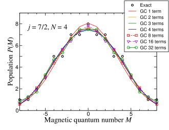
(a) $M$ distribution: exact and Gram-Charlier approximation. The Gram-Charlier expansion includes 1, 2, 3, 4, 8, 16 or 32 terms in the sum (VI.1).

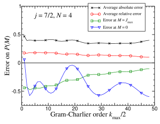
(b) Evaluation of the Gram-Charlier approximation. The average absolute and relative errors are defined in main text. The error at $M_{0}=J_{\text{max}}$ or $M_{0}=0$ is the value of the difference $P_{\text{GC}}(M_{0};k_{\text{max}})-P(M_{0})$ plotted as a function of the half truncation index $k_{\text{max}}/2$.

Figure 1: Exact and Gram-Charlier approximation for the magnetic quantum number $P(M)$ in the relativistic configuration $j=7/2$, $N=4$ (e.g., $4g_{7/2}^{4}$). The one-term computation is the Gaussian form, the 2-term form includes the $c_{4}$ contribution, i.e., the excess kurtosis, the 3-term form includes $c_{4}$ and $c_{6}$, etc.

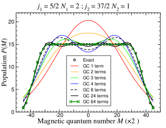
(a) $M$ distribution

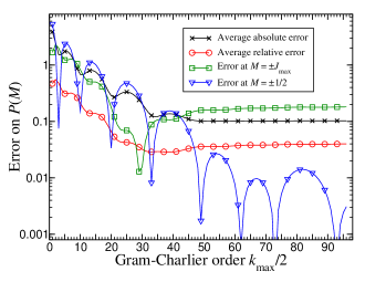
(b) Accuracy of Gram-Charlier approximation as a function of the “half-truncation order” $k/2$. See main text for the definitions.

Figure 2: Exact and Gram-Charlier approximations for the magnetic quantum number $P(M)$ in the relativistic configuration $j_{1}=5/2$ $N_{1}=2,j_{2}=37/2,N_{2}=1$.

Another interesting example is provided by $P(M)$ distributions exhibiting a wide plateau around $M=0$, which occur in configurations containing both high and low $j$ values. Configurations involving high-$j$ spectators are created for instance by electron capture into high-lying Rydberg states in collisions between multiply charged ions and light target gases [33]. Let us consider the configuration $j_{1}=5/2,N_{1}=2,j_{2}=37/2,N_{2}=1$ which is analogous to the case considered in Ref. [14]. The magnetic quantum number distribution for this case is plotted in Fig. 2(a). One notes that the first orders of the Gram-Charlier expansion provide a poor representation of the wide plateau extending from $M=-29/2$ to $M=29/2$. The quality of this approximation slowly improves with $k_{\text{max}}$, but obtaining a good agreement with the exact $P(M)$ distribution requires large $k_{\text{max}}$ values. The evolution of the accuracy with the truncation index in the Gram-Charlier series is quantitatively analyzed on Fig. 2. It appears that all the $P(M)$ values, including those for $M\simeq 0$ and $M\simeq\pm J_{\text{max}}$ are correctly described for a cut-off $k_{\text{max}}/2\simeq 40$. The average absolute error is then $0.28$, the average relative error is $0.066$, the error at $M=\pm J_{\text{max}}$ is $0.18$ and the error at $M=\pm 1/2$ is $-0.035$, which means that the relative error $|P_{\text{GC}}(M;k)/P(M)-1|$ is below 15% for any $M$. Above this $k$ value, adding more terms slightly improves the accuracy in the $M\simeq 0$ region, while the larger $|M|$ values are almost insensitive to these high-order terms. Though we did not develop a rigorous mathematical analysis, it appears that the Gram-Charlier series provides an asymptotic-type convergence: for a large range of $k_{\text{max}}$ values, the absolute error levels off at 0.28, and for very large truncation index, a divergence is expected.

VI.4 Example of large j and large N

One may note that several works in plasma physics or EBIT spectroscopy deal with ions involving almost half-filled d or f subshells [34, 35, 36]. Such subshells also deserve consideration in plasma sources for nanolithography [32, 37]. We have plotted the exact and Gram-Charlier distributions for $P(M)$ in the half-filled subshell $N=j+1/2$ with $j=15/2$ on Fig. 3(a), for which $J_{\text{max}}=32$. One observes that the Gram-Charlier approximation performs well on the whole $M$-range. In more detail the simple 1-term form is accurate everywhere except close to the $M=0$ region, and the 2-term form, including variance and kurtosis, provides a fair approximation whatever $M$. In order to get a more quantitative picture, we have plotted in Fig. 3(b) the various evaluations of the error done as a function of the half truncation index $k/2$. On this figure the errors at $M=\pm J_{\text{max}}$ or $M=0$ are indeed the absolute differences $|P_{\text{GC}}(M;k_{\text{max}})-P(M)|$ to allow for a logarithmic scale, but it is noticeable that, for both $M$ values, the sign of the differences $P_{\text{GC}}(M;k_{\text{max}})-P(M)$ is positive for $k_{\text{max}}=2$, and negative for higher $k$. It turns out that including terms in the Gram-Charlier expansion beyond $k=4$ brings little improvement in the analytical representation of $P(M)$. It is even surprising that the various plotted errors tend to some asymptotic value, namely one notes that, for $M=J_{\text{max}}$, one has $P_{\text{GC}}(M;k)-P(M)\rightarrow-0.4$ for large $k$, and for $M=0$ the “limit” is $\sim-2.5$ with some oscillations. Therefore the “convergence” of the Gram-Charlier series is really poor in this case, the two-term expansion including up to the excess kurtosis providing a fair approximation for such half-filled subshells. This agrees with the conclusions obtained previously by Bauche et al [12], though the effect of high-order terms was not quantitatively evaluated in this paper. Once again this case study suggests that the Gram-Charlier expansion provides an asymptotic representation of the magnetic momentum distribution.

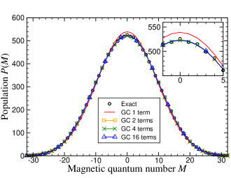
(a) $M$ distribution. For $k_{\text{max}}\geq 4$ the plots are almost indistinguishable at the drawing accuracy.

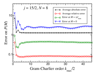
(b) Test of Gram-Charlier approximation as a function of the half-truncation order $k_{\text{max}}/2$. The green line with square symbols (resp. blue line with triangle symbols) is the absolute value $|P_{\text{GC}}(M;k_{\text{max}})-P(M)|$ for $M=\pm J_{\text{max}})$ (resp. $M=0$).

Figure 3: Exact and Gram-Charlier approximation for the magnetic quantum number $P(M)$ in the relativistic configuration $j=15/2$, $N=8$.

VI.5 Example of multiple subshells

It is not obvious to find situations where configurations with many open subshells contribute significantly to plasma spectra. However it is worth noting that the case of several singly-populated subshells is connected to the numbering of configurations contained in a superconfiguration analyzed in Ref. [25] because the cumulants are formally identical. Consequently, as a last illustration for the analysis of the $P(M)$ distribution we consider here a configuration with 10 subshells $j=1/2$–$19/2$, all containing a single electron. For this 10-electron configuration one has $J_{\text{max}}=50$, the degeneracy is $2^{10}.10!=3.7158912\times 10^{9}$, and the population $P(M)$ varies on 8 orders of magnitude. We have plotted in Fig. 4 the $P(M)$ distribution computed exactly and the differences between Gram-Charlier expansion truncated at various orders and the exact value. It turns out that the approximation with one term differs from the exact value, while Gram-Charlier approximation with at least 2 terms agrees with the exact value at the drawing accuracy. A more quantitative picture is provided by Figs 5(a) and 5(b). The former is a plot of the absolute and relative errors. The latter is the plot of the absolute difference between Gram-Charlier and exact values $\left|P_{\text{GC}}(M;k)-P(M)\right|$ for various $k$ values at $M=0$ and $M=J_{\text{max}}$. The differences $\left|P_{\text{GC}}(M;k)-P(M)\right|$ may also be divided by the exact $P(M)$ which are $P(0)=1.27707302\times 10^{8}$ and $P(J_{\text{max}})=1$ respectively. Therefore from Fig. 5(b) it appears that the relative accuracy is much better for $M=0$ than for $M=J_{\text{max}}$.

As seen on these figures, the description of the distribution $P(M)$ by the Gram-Charlier expansion improves continuously with $k_{\text{max}}$. With 16-byte floating point accuracy, we noticed a divergence on the absolute and relative errors for $k_{\text{max}}\simeq 64$, while such behavior disappears in the present computations using Mathematica software. One notes that using $k_{\text{max}}=5$, the gain in accuracy versus an approximation including only the kurtosis ($k_{\text{max}}=5$) is significant, which gives a certain interest to the present analysis.

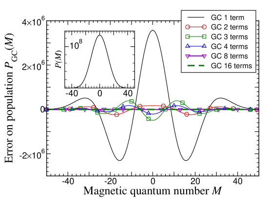
Figure 4: Difference between Gram-Charlier approximation at various orders and exact value for the distribution $P(M)$. The relativistic configuration analyzed consists of 10 subshells $j=1/2$–$19/2$, all containing a single electron. The inset shows the exact distribution.

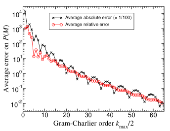
(a) Average error done in using the Gram-Charlier formula for the distribution $P(M)$ according to formulas (VI.7,VI.8)

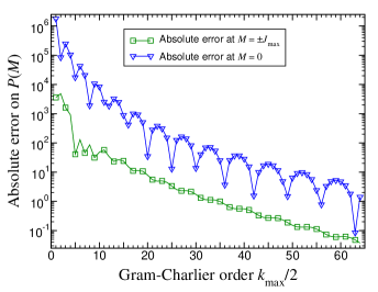
(b) Absolute error done in using the Gram-Charlier formula for the values $P(J_{\text{max}})$ and $P(0)$.

Figure 5: Analysis of the Gram-Charlier series convergence for the $P(M)$ distribution in the relativistic configuration with 10 subshells $j=1/2$–$19/2$, all containing a single electron.

VI.6 Convergence of the Gram-Charlier series

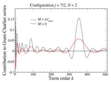
(a) Configuration $j=7/2,N=2$

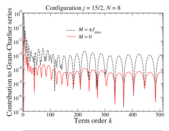
(b) Configuration $j=15/2,N=8$

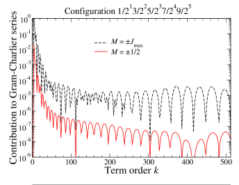
(c) Configuration with 5 subshells, $j_{i}=i-1/2,N_{i}=i$ ($i=$1–5)

Figure 6: Dependence of the generic term in the Gram-Charlier expansion $c_{k}He_{k}(M/\sigma)$ versus $k$ for three relativistic configurations and for two $M$ values. In the last two cases, the absolute value of this term is plotted in order to allow for logarithmic scale.

While we estimate the question of the mathematical convergence of the Gram-Charlier series to be outside the scope of this work, it is useful to check how the generic term of the sum in Eq. (VI.1) varies with $k$. To this respect, we have plotted in Fig. 6 the term $c_{k}He_{k}(M/\sigma)$ or its absolute value versus $k$ for the values $M=J_{\text{max}}$ and $M=0$ or $M=\pm 1/2$ for three configurations. Of course these computations were performed with arbitrary precision software to avoid inaccuracies when computing large-order coefficients. In Fig. 6(a) illustrating a 2-electron configuration case we notice that the $c_{k}He_{k}$ term oscillates with $k$ and do not decrease in absolute value below 0.1. For the more populated configurations shown in Fig. 6(b) (resp. 6(c)) the generic term of the series also oscillates and decreases to lower values. One notices a plateau in the oscillation amplitudes at $10^{-4}$ for $M=0$ (resp. $10^{-7}$ for $M=1/2$). However, as far as we could check, we did not observe a subsequent decrease of this generic term for greater $k$ values. These numerical considerations lead us to estimate that the Gram-Charlier series is probably not convergent, though accounting for a large number of terms may significantly improve the quality of this approximation, with better results for configurations with a large number of electrons. This behavior is characteristic of an asymptotic expansion.

VII Edgeworth series

VII.1 Definition

As mentioned by various authors [38, 39] some statistical distributions are better represented by Edgeworth series than by Gram-Charlier series. The Edgeworth distribution of the variable $X$ is naturally expressed in terms of cumulants, and is written as an expansion versus powers of the standard deviation

$$E(X)=G\frac{\exp(-x^{2}/2)}{\sqrt{2\pi}\sigma}\left[1+\sum_{s=1}^{\infty}\sigma^{s}\sum_{\{k_{m}\}}He_{s+2r}(x)\prod_{m=1}^{s}\frac{1}{k_{m}!}\left(\frac{S_{m+2}}{(m+2)!}\right)^{k_{m}}\right]$$ (VII.1a)

where we have introduced the reduced variable $$x=(X-\left<X\right>)/\sigma S_{n}=\kappa_{n}/\sigma^{2n-2} \{k_{m}\} s$$ and the modified cumulants . The set of indices refer to all -tuples verifying

$$r=k_{1}+k_{2}+\cdots k_{s}$$ (VII.1b)

$$k_{1}+2k_{2}+\cdots+sk_{s}=s,$$ (VII.1c)

i.e., partitions of the integer $s$. Since the analyzed distribution $P(M)$ is even, this series involves only even $s$ orders. An inspection of the above formulas shows that the $s=1$ contribution in the sum is proportional to the asymmetry $\kappa_{3}$ which cancels for the $P(M)$ distribution. The $s=2$ term is proportional to the excess kurtosis $\kappa_{4}$ and is identical to the first correction in the Gram-Charlier series. More generally one can check that the sum of coefficients factoring a polynomial of given order $He_{k}(x)$ in the expansion (VII.1a) is equal to the coefficient of the same order $c_{k}$ in the Gram-Charlier series. This property has been used to check the consistency of the coefficients in these expansions. It means that the Edgeworth series is indeed a rearrangement of the Gram-Charlier series, where each individual term is recast in various orders of the Edgeworth series.

VII.2 A test of Edgeworth accuracy

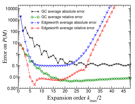
Figure 7: Absolute error and relative done in using the Gram-Charlier and Edgeworth formula for the $P(M)$ distribution. The analyzed configuration is $j_{1}=1/2,N_{1}=1,j_{2}=3/2,N_{2}=2,j_{3}=5/2,N_{3}=3,j_{4}=7/2,N_{4}=4,j_{5}=9/2,N_{5}=5$.

The relative efficiency of Edgeworth and Gram-Charlier series is illustrated in Fig. 7 for the configuration with 5 half-filled subshells $j_{1}=1/2,N_{1}=1,j_{2}=3/2,N_{2}=2,j_{3}=5/2,N_{3}=3,j_{4}=7/2,N_{4}=4,j_{5}=9/2,N_{5}=5$, where we have plotted the errors (VI.7) and (VI.8) for both series as functions of the half truncation index $k_{\text{max}}/2$. For the lowest $k_{\text{max}}$ values, the Edgeworth series provides a better approximation by a factor of 10. For greater values of this index, the Gram-Charlier expansion tends toward an acceptable approximation, with a relative error below 0.01. Conversely, the Edgeworth expansion is clearly divergent for $k_{\text{max}}\gtrsim 40$ or 50.

This expansion has been studied numerically using high-precision arithmetic in Fortran and arbitrary precision in Mathematica, which allows us to conclude that the divergence is not an artifact due to loss of accuracy in numerical computations but really a mathematical divergence. This behavior is similar to that observed for Gram-Charlier expansion, with two noticeable differences: the “best-convergence plateau” is reached earlier in the present case, and the onset of the divergence is also earlier and more pronounced here.

VIII Discussion and conclusion

We have studied in this paper various aspects of the statistics of the total quantum magnetic number distribution $P(M)$ in the most general relativistic configuration, accounting for the fermion character of the electrons. We have mentioned that atomic configurations considered here may be of importance in several domains such as plasma spectroscopy, nanolithography-source design or EBIT facilities. Up to our knowledge, there exists no compact analytical expression for the quantum magnetic number distribution, which justifies the present effort. Using the cumulant generating function formalism we have derived a recurrence relation for this function connecting four adjacent $j$ and $N$ values in the case of a single subshell $j^{N}$. This relation allowed us to establish a compact analytical expression for the cumulant generating function, which is straightforwardly generalized to a relativistic configuration with any subshell number. In the case of a single subshell this generating function allows us to express $P(M)$ as a n-th derivative. This formal property leads to two recurrence relations on $P(M)$ for adjacent $N$ or $j$, $j$ being allowed to span integer as well as half-integer values. Such recurrences prove to be quite efficient in obtaining the whole $P(M)$ distribution for complex configurations. We have been able to express the cumulants of the $P(M)$ distribution at any order for the most general relativistic configuration. This allowed us to build a Gram-Charlier approximation of the magnetic quantum number distribution at any order. The Gram-Charlier analysis performed here has provided a variety of results. First, it has been stressed that the handling of series with several tens of terms requires the use of arbitrary precision, since a “divergence” due to a loss of numerical accuracy may be observed for a $k_{\text{max}}\sim 40$. For a subshell with significant population — e.g., an half-filled subshell with large $j$ — the first two terms of the expansion provide a very good approximation while adding many more terms do not improve the approximation at all. Conversely, in the cases with a large number of subshells each one with a small population, the quality of the Gram-Charlier expansion improves as more terms are added. Similar conclusions holds for “exotic” configurations for which the $M$-distribution shows a broad plateau, which can be fairly reproduced by including several tens of terms.

It has been verified that configurations with a large number of electrons are better represented by Edgeworth expansion for a moderate value of the truncation index, reaching a best-approximation plateau before the Gram-Charlier expansion. Furthermore, a better accuracy is achieved for configurations with a large number of electrons. However both expansions appear to be asymptotic and not convergent, with an earlier divergence for the Edgeworth series. Such conclusions are similar to what we obtained when considering the statistics of configurations inside a superconfiguration. A physically important application of this analysis is that it leads to useful information on the distribution of total angular momentum $J$ and on line numbers. This will be considered in a forthcoming paper.

Appendix A Alternate proposal for a derivation of the expression of the cumulant generating function

In order to prove the general expression (II.18) one may directly establish the two-term relation (II.23) with

$$s_{N}(t)=\sum_{M}P(M)e^{Mt}=\sum_{m_{1}<m_{2}<\cdots<m_{N}}e^{(m_{1}+\cdots+m_{N})t}.$$ (A.1)

The recurrence (II.23) may be written

$$\left(e^{(j+1-N/2)t}-e^{-(j+1-N/2)t}\right)s_{N-1}(t)=\left(e^{Nt/2}-e^{-Nt/2}\right)s_{N}(t)$$ (A.2)

or after some elementary transformation

$$\left(e^{-(j+1-N)t}+e^{-(j-N)t}+\cdots+e^{jt}\right)s_{N-1}(t)=\left(1+e^{t}+\cdots+e^{(N-1)t}\right)s_{N}(t).$$ (A.3)

The left member contains $(2j+2-N)\binom{2j+1}{N-1}$ terms and the right member contains $N\binom{2j+1}{N}$ terms which are both equal. A detailed inspection of the terms in both members shows that they are indeed identical. However this verification is somewhat tedious and the proof given in Section II is easier to establish.

Appendix B Derivation of recurrence relations using generalized Pascal-triangle relations for the Gaussian binomial coefficients

From the definition of the Gaussian binomial coefficients (III.3), after elementary algebraic operations, we get the well-known triangle-like relation

$$\left[\begin{array}[]{c}2j+1\\ N\end{array}\right]_{z}=z^{N}\left[\begin{array}[]{c}2j\\ N\end{array}\right]_{z}+\left[\begin{array}[]{c}2j\\ N-1\end{array}\right]_{z}$$ (B.1)

and, deriving this equation $n$ times versus $z$ using the Leibniz rule, we obtain

$$\left.\frac{\partial^{n}}{\partial z^{n}}\left[\begin{array}[]{c}2j+1\\ N\end{array}\right]_{z}\right|_{z=0}=\left.\sum_{k=0}^{N}\binom{n}{k}\frac{\partial^{n-k}}{\partial z^{n-k}}z^{N}.\frac{\partial^{k}}{\partial z^{k}}\left[\begin{array}[]{c}2j\\ N\end{array}\right]_{z}\right|_{z=0}+\left.\frac{\partial^{n}}{\partial z^{n}}\left[\begin{array}[]{c}2j\\ N-1\end{array}\right]_{z}\right|_{z=0}.$$ (B.2)

From the value of the n-th derivative of $z^{N}$ at the origin, and after dividing by $n!$, we get

$$\frac{1}{n!}\left.\frac{\partial^{n}}{\partial z^{n}}\left[\begin{array}[]{c}2j+1\\ N\end{array}\right]_{z}\right|_{z=0}=\left.\frac{1}{(n-N)!}.\left.\frac{\partial^{n-N}}{\partial z^{n-N}}\left[\begin{array}[]{c}2j\\ N\end{array}\right]_{z}\right|_{z=0}+\frac{1}{n!}\frac{\partial^{n}}{\partial z^{n}}\left[\begin{array}[]{c}2j\\ N-1\end{array}\right]_{z}\right|_{z=0},$$ (B.3)

so that, with the definition (III.7) of $P(M)$ as a multiple derivative and the substitution $M=n-N(2j+1-N)/2$,

$$P(M;j,N)=P\left(M-\frac{N}{2};j-\frac{1}{2},N\right)+P\left(M+\frac{2j+1-N}{2};j-\frac{1}{2},N-1\right).$$ (B.4)

With $0\leq n\leq 2J_{\mathrm{max}}$, using the notation $\mathscr{P}_{j,N}(n)$ introduced in Eq. (III.14), we obtain

$$\mathscr{P}_{j,N}\left(n\right)=\mathscr{P}_{j-1/2,N}\left(n-N\right)+\mathscr{P}_{j-1/2,N-1}\left(n\right).$$ (B.5)

It is also quite simple to derive from the definition (III.3) another triangle-like equation

$$\left[\begin{array}[]{c}2j+1\\ N\end{array}\right]_{z}=\left[\begin{array}[]{c}2j\\ N\end{array}\right]_{z}+z^{2j+1-N}\left[\begin{array}[]{c}2j\\ N-1\end{array}\right]_{z}$$ (B.6)

and therefore, applying the same procedure as above, we get

$$\left.\frac{\partial^{n}}{\partial z^{n}}\left[\begin{array}[]{c}2j+1\\ N\end{array}\right]_{z}\right|_{z=0}=\left.\frac{\partial^{n}}{\partial z^{n}}\left[\begin{array}[]{c}2j\\ N\end{array}\right]_{z}\right|_{z=0}+\left.\binom{n}{2j+1-N}\frac{\partial^{2j+1-N}}{\partial z^{2j+1-N}}z^{2j+1-N}.\frac{\partial^{n-2j-1+N}}{\partial z^{n-2j-1+N}}\left[\begin{array}[]{c}2j\\ N-1\end{array}\right]_{z}\right|_{z=0},$$ (B.7)

i.e.

$$P(M;j,N)=P\left(M+\frac{N}{2};j-\frac{1}{2},N\right)+P\left(M-\frac{2j+1-N}{2};j-\frac{1}{2},N-1\right).$$ (B.8)

Since the distribution $P(M)$ is even, one easily checks that this recurrence relation is indeed equivalent to the previous one (B.4). With $0\leq n\leq 2J_{\mathrm{max}}$ and using the $\mathscr{P}_{j,N}$ notation, we obtain

$$\mathscr{P}_{j,N}\left(n\right)=\mathscr{P}_{j-1/2,N}\left(n\right)+\mathscr{P}_{j-1/2,N-1}\left(n-2j-1+N\right).$$ (B.9)

Combining Eqs. (B.5) and (B.9), one gets

$$\mathscr{P}_{j-1/2,N}\left(n-N\right)+\mathscr{P}_{j-1/2,N-1}\left(n\right)=\mathscr{P}_{j-1/2,N}\left(n\right)+\mathscr{P}_{j-1/2,N-1}\left(n-2j-1+N\right),$$ (B.10)

which is exactly the recurrence relation over $N$ (III.15) with the substitution $j\rightarrow j-1/2$. Similarly, making the substitution $n\rightarrow n-2j-1+N$ in Eq. (B.5), we get

$$\mathscr{P}_{j-1/2,N-1}\left(n-2j-1+N\right)=\mathscr{P}_{j,N}\left(n-2j-1+N\right)-\mathscr{P}_{j-1/2,N}\left(n-2j-1\right).$$ (B.11)

Combining Eq. (B.9) with Eq. (B.11) yields exactly the recurrence relation over $j$ (III.22).

Appendix C Explicit values for the moments in a relativistic configuration

The explicit value for the cumulants (IV.5) and the relation between moments and cumulants (IV.12) shows that the polynomial form of the moments inside a $j^{N}$-subshell is written as

$$\mu_{2k}=\sum_{p=1}^{k}M(2k,p)\left[N(2j+1-N)\right]^{p}.$$ (C.1)

The first values for $M(2k,p)$ are listed below.

$$M(2,1) =\frac{j+1}{6}$$ (C.2a)

$$M(4,1) =-\frac{1}{30}(j+1)^{2}(2j+1)$$ (C.2b)

$$M(4,2) =\frac{1}{60}(j+1)(5j+6)$$ (C.2c)

$$M(6,1) =\frac{1}{126}(j+1)^{2}(2j+1)\left(8j^{2}+12j+3\right)$$ (C.2d)

$$M(6,2) =-\frac{1}{252}(j+1)(2j+1)\left(21j^{2}+50j+30\right)$$ (C.2e)

$$M(6,3) =\frac{1}{504}(j+1)\left(35j^{2}+91j+60\right)$$ (C.2f)

$$M(8,1) =-\frac{1}{90}(j+1)^{2}(2j+1)\left(24j^{4}+72j^{3}+70j^{2}+24j+3\right)$$ (C.2g)

$$M(8,2) =\frac{1}{540}(j+1)(2j+1)\left(202j^{4}+815j^{3}+1177j^{2}+693j+126\right)$$ (C.2h)

$$M(8,3) =-\frac{1}{540}(j+1)(2j+1)(3j+4)\left(35j^{2}+92j+63\right)$$ (C.2i)

$$M(8,4) =\frac{1}{2160}(j+1)(5j+7)\left(35j^{2}+98j+72\right)$$ (C.2j)

$$M(10,1) =\frac{1}{66}(j+1)^{2}(2j+1)\left(4j^{2}+6j+1\right)\left(32j^{4}+96j^{3}+92j^{2}+30j+5\right)$$ (C.2k)

$$M(10,2) =-\frac{1}{396}(j+1)(2j+1)\left(1144j^{6}+6488j^{5}+14634j^{4}+16450j^{3}+9419j^{2}+2520j+270\right)$$ (C.2l)

$$M(10,3) =\frac{1}{792}(j+1)(2j+1)\left(1342j^{5}+7755j^{4}+17546j^{3}+19076j^{2}+9599j+1620\right)$$ (C.2m)

$$M(10,4) =-\frac{1}{792}(j+1)(2j+1)\left(385j^{4}+2211j^{3}+4840j^{2}+4784j+1800\right)$$ (C.2n)

$$M(10,5) =\frac{1}{3168}(j+1)\left(385j^{4}+2310j^{3}+5291j^{2}+5478j+2160\right)$$ (C.2o)

$$M(12,1) =-\frac{691}{8190}(j+1)^{2}(2j+1)$$

$$\quad\times\left(256j^{8}+1536j^{7}+3712j^{6}+4608j^{5}+3160j^{4}+1272j^{3}+338j^{2}+48j+3\right)$$ (C.2p)

$$M(12,2) =\frac{1}{49140}(j+1)(2j+1)$$

$$\quad\times\left(1663792j^{8}+12141368j^{7}+37081404j^{6}+60997498j^{5}+58017896j^{4}\right.$$

$$\qquad\left.+32097489j^{3}+10156029j^{2}+1829949j+136818\right)$$ (C.2q)

$$M(12,3) =-\frac{1}{98280}(j+1)(2j+1)$$

$$\quad\times\left(2126124j^{7}+16084328j^{6}+50719883j^{5}+85218445j^{4}+80675641j^{3}\right.$$

$$\qquad\left.+41715213j^{2}+10549422j+1094544\right)$$ (C.2r)

$$M(12,4) =\frac{1}{196560}(j+1)(2j+1)\left(1431430j^{6}+11062051j^{5}+35328306j^{4}\right.$$

$$\quad\left.+59068682j^{3}+53560409j^{2}+24090798j+3830904\right)$$ (C.2s)

$$M(12,5) =-\frac{1}{393120}(j+1)(2j+1)$$

$$\quad\times\left(525525j^{5}+4059055j^{4}+12765753j^{3}+20419373j^{2}+16593534j+5472720\right)$$ (C.2t)

$$M(12,6) =\frac{1}{786240}(j+1)$$

$$\quad\times\left(175175j^{5}+1401400j^{4}+4569565j^{3}+7583576j^{2}+6396156j+2189088\right)$$ (C.2u)

One notes that as a rule the moments exhibit a more complex expression than the cumulants.

Appendix D A recurrence relation on the distribution moments

From the expressions of the moments (IV.11) and of the generating function (II.11) one gets the non-normalized moments

$$\mathscr{M}_{k}(j^{N})=\binom{2j+1}{N}\mu_{k}=\left.\frac{\partial^{k}}{\partial t^{k}}s(N,j,t)\right|_{t=0}.$$ (D.1)

After deriving Eq. (V.4) $k$ times versus $t$ using the Leibniz rule, one gets the relation

$$\mathscr{M}_{k}(j^{N})=\frac{1}{N}\sum_{p=1}^{N}(-1)^{p-1}\sum_{q=0}^{k}\binom{k}{q}p^{k-q}\mathscr{M}_{q}(j^{N-p})\mathscr{M}_{k-q}(j^{1})$$ (D.2)

and for the normalized moments

$$\mu_{k}(j^{N})=\frac{2j+1}{N}\sum_{p=1}^{N}(-1)^{p-1}\frac{N!(2j+1-N)!}{(N-p)!(2j+1-N+p)!}\sum_{q=0}^{k}\binom{k}{q}p^{k-q}\mu_{q}(j^{N-p})\mu_{k-q}(j^{1})$$ (D.3)

which indeed involves only even indices $k,q$. In the above equations one must define the moments for the empty subshell $j^{0}$, which are $\mathscr{M}_{s}(j^{0})=\mu_{s}(j^{0})=0$ if $s>0$, and $\mathscr{M}_{0}(j^{0})=\mu_{0}(j^{0})=1$. The even-order moments for a single-electron subshell $j^{1}$, defined as $\mathscr{M}_{2k}(j^{1})=\sum_{m=-j}^{j}m^{2k}$ are simply related to Bernoulli numbers $B_{n}(x)$

$$\mathscr{M}_{2k}(j^{1})=\frac{B_{2k+1}(j+1)-B_{2k}(-j)}{2k+1}.$$ (D.4)

References

- Bethe [1936] H. A. Bethe, An attempt to calculate the number of energy levels of a heavy nucleus, Phys. Rev. 50, 332 (1936).
- Cowan [1981] R. D. Cowan, The Theory of Atomic Structure and Spectra, Los Alamos Series in Basic and Applied Sciences (University of California Press, Ltd., Berkeley, 1981).
- Judd [1968] B. R. Judd, Atomic term patterns, Phys. Rev. 173, 39 (1968).
- Breit [1926] G. Breit, An application of Pauli’s method of coordination to atoms having four magnetic parts, Phys. Rev. 28, 334 (1926).
- Curl and Kilpatrick [1960] R. F. Curl and J. E. Kilpatrick, Atomic term symbols by group theory, Am. J. Phys. 28, 357 (1960).
- Karayianis [1965] N. Karayianis, Atomic terms for equivalent electrons, J. Math. Phys. 6, 1204 (1965).
- Katriel and Novoselsky [1989] J. Katriel and A. Novoselsky, Term multiplicities in the LS-coupling scheme, J. Phys. A: Math. Gen. 22, 1245 (1989).
- Xu and Dai [2006] R. Xu and Z. Dai, Alternative mathematical technique to determine LS spectral terms, J. Phys. B: At. Mol. Opt. Phys. 39, 3221 (2006).
- Bauche et al. [1988] J. Bauche, C. Bauche-Arnoult, and M. Klapisch, Transition arrays in the spectra of ionized atoms, Adv. At. Mol. Phys. 23, 131 (1988).
- Moszkowski [1960] S. A. Moszkowski, Some statistical properties of level and line distributions in atomic spectra, Tech. Rep. (RAND Corp., Santa Monica, California, 1960).
- Bancewicz and Karwowski [1984] M. Bancewicz and J. Karwowski, A study on atomic energy level distribution, Acta Phys. Pol. Ser. A 65, 279 (1984).
- Bauche and Bauche-Arnoult [1987] J. Bauche and C. Bauche-Arnoult, Level and line statistic in atomic spectra, J. Phys. B: At. Mol. Opt. Phys. 20, 1659 (1987).
- Bauche and Bauche-Arnoult [1990] J. Bauche and C. Bauche-Arnoult, Statistical properties of atomic spectra, Comp. Phys. Rep. 12, 1 (1990).
- Gilleron and Pain [2009] F. Gilleron and J.-C. Pain, Efficient methods for calculating the number of states, levels and lines in atomic configurations, High Energy Density Phys. 5, 320 (2009).
- Porcherot et al. [2011] Q. Porcherot, J.-C. Pain, F. Gilleron, and T. Blenski, A consistent approach for mixed detailed and statistical calculation of opacities in hot plasmas, High Energy Density Phys. 7, 234 (2011).
- Pain et al. [2012] J.-C. Pain, F. Gilleron, J. Bauche, and C. Bauche-Arnoult, Statistics of electric-quadrupole lines in atomic spectra, J. Phys. B: At. Mol. Opt. Phys. 45, 135006 (2012).
- Bauche and Cossé [1997] J. Bauche and P. Cossé, Odd-even staggering in the J and L distributions of atomic configurations, J. Phys. B: At. Mol. Opt. Phys. 30, 1411 (1997).
- Pain [2013] J.-C. Pain, Regularities and symmetries in atomic structure and spectra, High Energy Density Phys. 9, 392 (2013).
- Moszkowski [1962] S. A. Moszkowski, On the energy distribution of terms and line arrays in atomic spectra, Progr. Theor. Phys. 28, 1 (1962).
- Ginocchio [1973] J. N. Ginocchio, Operator averages in a shell-model basis, Phys. Rev. C 8, 135 (1973).
- Karazija [1991] R. Karazija, Evaluation of explicit expressions for mean characteristics of atomic spectra, Acta Phys. Hung. 70, 367 (1991).
- Kučas et al. [1995] S. Kučas, V. Jonauskas, R. Karazija, and I. Martinson, Global characteristics of atomic spectra and their use for the analysis of spectra. II. characteristic emission spectra, Phys. Scr. 51, 566 (1995).
- Gilleron et al. [2008] F. Gilleron, J. C. Pain, J. Bauche, and C. Bauche-Arnoult, Impact of high-order moments on the statistical modeling of transition arrays, Phys. Rev. E 77, 026708 (2008).
- Kyniėne et al. [2002] A. Kyniėne, R. Karazija, and V. Jonauskas, Statistical properties of Auger amplitudes and rates, J. Electron Spectrosc. Relat. Phenom. 122, 181 (2002).
- Pain and Poirier [2020] J.-C. Pain and M. Poirier, Analytical and numerical expressions for the number of atomic configurations contained in a supershell, J. Phys. B: At. Mol. Opt. Phys. 53, 115002 (2020).
- Condon and Shortley [1935] E. U. Condon and G. H. Shortley, The theory of atomic spectra (Cambridge University Press, Cambridge, UK, 1935).
- Stuart and Ord [1994] A. Stuart and J. K. Ord, Kendall’s Advanced Theory of Statistics – Distribution Theory, Vol. 1 (John Wiley and Sons, London UK, 1994).
- Talmi [2005] I. Talmi, Number of states with given spin of fermions in a orbit, Phys. Rev. C 72, 037302 (2005).
- Andrews [1984] G. E. Andrews, The Theory of Partitions, Encyclopedia of Mathematics and its Applications (Cambridge University Press, 1984).
- Abramowitz and Stegun [1972] M. Abramowitz and I. Stegun, Handbook of Mathematical Functions (National Bureau of Standards, Washington DC, USA, 1972).
- Ginocchio and Yen [1975] J. Ginocchio and M. Yen, The dependence of shell model state densities on angular momentum, Nucl. Phys. A 239, 365 (1975).
- Shevelko et al. [1998] A. P. Shevelko, L. A. Shmaenok, S. S. Churilov, R. K. F. J. Bastiaensen, and F. Bijkerk, Extreme ultraviolet spectroscopy of a laser plasma source for lithography, Phys. Scr. 57, 276 (1998).
- Hvelplund et al. [1981] P. Hvelplund, H. K. Haugen, H. Knudsen, L. Andersen, H. Damsgaard, and F. Fukusawa, Electron capture into high-lying Rydberg states in collisions between multiply charged ions and H2, Phys. Scr. 24, 40 (1981).
- Zigler et al. [1987] A. Zigler, M. Givon, E. Yarkoni, M. Kishinevsky, E. Goldberg, B. Arad, and M. Klapisch, Use of unresolved transition arrays for plasma diagnostics, Phys. Rev. A 35, 280 (1987).
- Radtke et al. [2001] R. Radtke, C. Biedermann, J. L. Schwob, P. Mandelbaum, and R. Doron, Line and band emission from tungsten ions with charge to in the 45–70-Å range, Phys. Rev. A 64, 012720 (2001).
- Jonauskas et al. [2012] V. Jonauskas, A. Kynienė, R. Kisielius, and Š. Masys, Theoretical study of W20+ spectra formation in EBIT plasma, J. Phys. Conf. Ser. 388, 042016 (2012).
- O’Sullivan et al. [2015] G. O’Sullivan, P. Dunne, T. Higashiguchi, B. Li, L. Liu, R. Lokasani, E. Long, H. Ohashi, F. O’Reilly, P. Sheridan, E. Sokell, C. Suzuki, and T. Wu, Spectroscopy for identification of plasma sources for lithography and water window imaging, J. Phys. Conf. Ser. 635, 012026 (2015).
- Blinnikov and Moessner [1998] S. Blinnikov and R. Moessner, Expansions for nearly Gaussian distributions, Astron. Astrophys. Suppl. Ser. 130, 193 (1998).
- de Kock et al. [2011] M. B. de Kock, H. C. Eggers, and J. Schmiegel, Edgeworth versus Gram-Charlier series: x-cumulant and probability density tests, Phys. Part. Nucl. Lett. 8, 1023 (2011).