Autoformer: Decomposition Transformers with
Auto-Correlation for Long-Term Series Forecasting

Abstract

Extending the forecasting time is a critical demand for real applications, such as extreme weather early warning and long-term energy consumption planning. This paper studies the long-term forecasting problem of time series. Prior Transformer-based models adopt various self-attention mechanisms to discover the long-range dependencies. However, intricate temporal patterns of the long-term future prohibit the model from finding reliable dependencies. Also, Transformers have to adopt the sparse versions of point-wise self-attentions for long series efficiency, resulting in the information utilization bottleneck. Going beyond Transformers, we design Autoformer as a novel decomposition architecture with an Auto-Correlation mechanism. We break with the pre-processing convention of series decomposition and renovate it as a basic inner block of deep models. This design empowers Autoformer with progressive decomposition capacities for complex time series. Further, inspired by the stochastic process theory, we design the Auto-Correlation mechanism based on the series periodicity, which conducts the dependencies discovery and representation aggregation at the sub-series level. Auto-Correlation outperforms self-attention in both efficiency and accuracy. In long-term forecasting, Autoformer yields state-of-the-art accuracy, with a 38% relative improvement on six benchmarks, covering five practical applications: energy, traffic, economics, weather and disease. Code is available at this repository: https://github.com/thuml/Autoformer.

1 Introduction

Time series forecasting has been widely used in energy consumption, traffic and economics planning, weather and disease propagation forecasting. In these real-world applications, one pressing demand is to extend the forecast time into the far future, which is quite meaningful for the long-term planning and early warning. Thus, in this paper, we study the long-term forecasting problem of time series, characterizing itself by the large length of predicted time series. Recent deep forecasting models [48, 23, 26, 34, 29, 35, 25, 41] have achieved great progress, especially the Transformer-based models. Benefiting from the self-attention mechanism, Transformers obtain great advantage in modeling long-term dependencies for sequential data, which enables more powerful big models [8, 13].

However, the forecasting task is extremely challenging under the long-term setting. First, it is unreliable to discover the temporal dependencies directly from the long-term time series because the dependencies can be obscured by entangled temporal patterns. Second, canonical Transformers with self-attention mechanisms are computationally prohibitive for long-term forecasting because of the quadratic complexity of sequence length. Previous Transformer-based forecasting models [48, 23, 26] mainly focus on improving self-attention to a sparse version. While performance is significantly improved, these models still utilize the point-wise representation aggregation. Thus, in the process of efficiency improvement, they will sacrifice the information utilization because of the sparse point-wise connections, resulting in a bottleneck for long-term forecasting of time series.

To reason about the intricate temporal patterns, we try to take the idea of decomposition, which is a standard method in time series analysis [1, 33]. It can be used to process the complex time series and extract more predictable components. However, under the forecasting context, it can only be used as the pre-processing of past series because the future is unknown [20]. This common usage limits the capabilities of decomposition and overlooks the potential future interactions among decomposed components. Thus, we attempt to go beyond pre-processing usage of decomposition and propose a generic architecture to empower the deep forecasting models with immanent capacity of progressive decomposition. Further, decomposition can ravel out the entangled temporal patterns and highlight the inherent properties of time series [20]. Benefiting from this, we try to take advantage of the series periodicity to renovate the point-wise connection in self-attention. We observe that the sub-series at the same phase position among periods often present similar temporal processes. Thus, we try to construct a series-level connection based on the process similarity derived by series periodicity.

Based on the above motivations, we propose an original Autoformer in place of the Transformers for long-term time series forecasting. Autoformer still follows residual and encoder-decoder structure but renovates Transformer into a decomposition forecasting architecture. By embedding our proposed decomposition blocks as the inner operators, Autoformer can progressively separate the long-term trend information from predicted hidden variables. This design allows our model to alternately decompose and refine the intermediate results during the forecasting procedure. Inspired by the stochastic process theory [9, 30], Autoformer introduces an Auto-Correlation mechanism in place of self-attention, which discovers the sub-series similarity based on the series periodicity and aggregates similar sub-series from underlying periods. This series-wise mechanism achieves $\mathcal{O}(L\log L)$ complexity for length-$L$ series and breaks the information utilization bottleneck by expanding the point-wise representation aggregation to sub-series level. Autoformer achieves the state-of-the-art accuracy on six benchmarks. The contributions are summarized as follows:

• To tackle the intricate temporal patterns of the long-term future, we present Autoformer as a decomposition architecture and design the inner decomposition block to empower the deep forecasting model with immanent progressive decomposition capacity.

• We propose an Auto-Correlation mechanism with dependencies discovery and information aggregation at the series level. Our mechanism is beyond previous self-attention family and can simultaneously benefit the computation efficiency and information utilization.

• Autoformer achieves a 38% relative improvement under the long-term setting on six benchmarks, covering five real-world applications: energy, traffic, economics, weather and disease.

2 Related Work

2.1 Models for Time Series Forecasting

Due to the immense importance of time series forecasting, various models have been well developed. Many time series forecasting methods start from the classic tools [38, 10]. ARIMA [7, 6] tackles the forecasting problem by transforming the non-stationary process to stationary through differencing. The filtering method is also introduced for series forecasting [24, 12]. Besides, recurrent neural networks (RNNs) models are used to model the temporal dependencies for time series [42, 32, 47, 28]. DeepAR [34] combines autoregressive methods and RNNs to model the probabilistic distribution of future series. LSTNet [25] introduces convolutional neural networks (CNNs) with recurrent-skip connections to capture the short-term and long-term temporal patterns. Attention-based RNNs [46, 36, 37] introduce the temporal attention to explore the long-range dependencies for prediction. Also, many works based on temporal convolution networks (TCN) [40, 5, 4, 35] attempt to model the temporal causality with the causal convolution. These deep forecasting models mainly focus on the temporal relation modeling by recurrent connections, temporal attention or causal convolution.

Recently, Transformers [41, 45] based on the self-attention mechanism shows great power in sequential data, such as natural language processing [13, 8], audio processing [19] and even computer vision [16, 27]. However, applying self-attention to long-term time series forecasting is computationally prohibitive because of the quadratic complexity of sequence length $L$ in both memory and time. LogTrans [26] introduces the local convolution to Transformer and proposes the LogSparse attention to select time steps following the exponentially increasing intervals, which reduces the complexity to $\mathcal{O}(L(\log L)^{2})$. Reformer [23] presents the local-sensitive hashing (LSH) attention and reduces the complexity to $\mathcal{O}(L\log L)$. Informer [48] extends Transformer with KL-divergence based ProbSparse attention and also achieves $\mathcal{O}(L\log L)$ complexity. Note that these methods are based on the vanilla Transformer and try to improve the self-attention mechanism to a sparse version, which still follows the point-wise dependency and aggregation. In this paper, our proposed Auto-Correlation mechanism is based on the inherent periodicity of time series and can provide series-wise connections.

2.2 Decomposition of Time Series

As a standard method in time series analysis, time series decomposition [1, 33] deconstructs a time series into several components, each representing one of the underlying categories of patterns that are more predictable. It is primarily useful for exploring historical changes over time. For the forecasting tasks, decomposition is always used as the pre-processing of historical series before predicting future series [20, 2], such as Prophet [39] with trend-seasonality decomposition and N-BEATS [29] with basis expansion and DeepGLO [35] with matrix decomposition. However, such pre-processing is limited by the plain decomposition effect of historical series and overlooks the hierarchical interaction between the underlying patterns of series in the long-term future. This paper takes the decomposition idea from a new progressive dimension. Our Autoformer harnesses the decomposition as an inner block of deep models, which can progressively decompose the hidden series throughout the whole forecasting process, including both the past series and the predicted intermediate results.

3 Autoformer

The time series forecasting problem is to predict the most probable length-$O$ series in the future given the past length-$I$ series, denoting as input-$I$-predict-$O$. The long-term forecasting setting is to predict the long-term future, i.e. larger $O$. As aforementioned, we have highlighted the difficulties of long-term series forecasting: handling intricate temporal patterns and breaking the bottleneck of computation efficiency and information utilization. To tackle these two challenges, we introduce the decomposition as a builtin block to the deep forecasting model and propose Autoformer as a decomposition architecture. Besides, we design the Auto-Correlation mechanism to discover the period-based dependencies and aggregate similar sub-series from underlying periods.

3.1 Decomposition Architecture

We renovate Transformer [41] to a deep decomposition architecture (Figure 1), including the inner series decomposition block, Auto-Correlation mechanism, and corresponding Encoder and Decoder.

Series decomposition block

To learn with the complex temporal patterns in long-term forecasting context, we take the idea of decomposition [1, 33], which can separate the series into trend-cyclical and seasonal parts. These two parts reflect the long-term progression and the seasonality of the series respectively. However, directly decomposing is unrealizable for future series because the future is just unknown. To tackle this dilemma, we present a series decomposition block as an inner operation of Autoformer (Figure 1), which can extract the long-term stationary trend from predicted intermediate hidden variables progressively. Concretely, we adapt the moving average to smooth out periodic fluctuations and highlight the long-term trends. For length-$L$ input series $\mathcal{X}\in\mathbb{R}^{L\times d}$, the process is:

$$\begin{split}\mathcal{X}_{\mathrm{t}}&=\mathrm{AvgPool}(\mathrm{Padding}(\mathcal{X}))\\ \mathcal{X}_{\mathrm{s}}&=\mathcal{X}-\mathcal{X}_{\mathrm{t}},\\ \end{split}$$ (1)

where $\mathcal{X}_{\mathrm{s}},\mathcal{X}_{\mathrm{t}}\in\mathbb{R}^{L\times d}$ denote the seasonal and the extracted trend-cyclical part respectively. We adopt the $\mathrm{AvgPool}(\cdot)$ for moving average with the padding operation to keep the series length unchanged. We use $\mathcal{X}_{\mathrm{s}},\mathcal{X}_{\mathrm{t}}=\mathrm{SeriesDecomp}(\mathcal{X})$ to summarize above equations, which is a model inner block.

Model inputs

The inputs of encoder part are the past $I$ time steps $\mathcal{X}_{\mathrm{en}}\in\mathbb{R}^{I\times d}$. As a decomposition architecture (Figure 1), the input of Autoformer decoder contains both the seasonal part $\mathcal{X}_{\mathrm{des}}\in\mathbb{R}^{(\frac{I}{2}+O)\times d}$ and trend-cyclical part $\mathcal{X}_{\mathrm{det}}\in\mathbb{R}^{(\frac{I}{2}+O)\times d}$ to be refined. Each initialization consists of two parts: the component decomposed from the latter half of encoder’s input $\mathcal{X}_{\mathrm{en}}$ with length $\frac{I}{2}$ to provide recent information, placeholders with length $O$ filled by scalars. It’s formulized as follows:

$$\begin{split}\mathcal{X}_{\mathrm{ens}},\mathcal{X}_{\mathrm{ent}}&=\mathrm{SeriesDecomp}({\mathcal{X}_{\mathrm{en}}}_{\frac{I}{2}:I})\\ \mathcal{X}_{\mathrm{des}}&=\mathrm{Concat}(\mathcal{X}_{\mathrm{ens}},\mathcal{X}_{0})\\ \mathcal{X}_{\mathrm{det}}&=\mathrm{Concat}(\mathcal{X}_{\mathrm{ent}},\mathcal{X}_{\mathrm{Mean}}),\\ \end{split}$$ (2)

where $\mathcal{X}_{\mathrm{ens}},\mathcal{X}_{\mathrm{ent}}\in\mathbb{R}^{\frac{I}{2}\times d}$ denote the seasonal and trend-cyclical parts of $\mathcal{X}_{\mathrm{en}}$ respectively, and $\mathcal{X}_{0},\mathcal{X}_{\mathrm{Mean}}\in\mathbb{R}^{O\times d}$ denote the placeholders filled with zero and the mean of $\mathcal{X}_{\mathrm{en}}$ respectively.

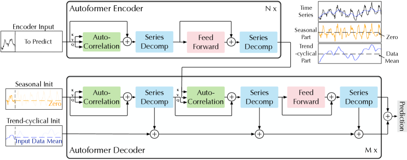
Figure 1: Autoformer architecture. The encoder eliminates the long-term trend-cyclical part by series decomposition blocks (blue blocks) and focuses on seasonal patterns modeling. The decoder accumulates the trend part extracted from hidden variables progressively. The past seasonal information from encoder is utilized by the encoder-decoder Auto-Correlation (center green block in decoder).

Encoder

As shown in Figure 1, the encoder focuses on the seasonal part modeling. The output of the encoder contains the past seasonal information and will be used as the cross information to help the decoder refine prediction results. Suppose we have $N$ encoder layers. The overall equations for $l$-th encoder layer are summarized as $\mathcal{X}_{\mathrm{en}}^{l}=\mathrm{Encoder}(\mathcal{X}_{\mathrm{en}}^{l-1})$. Details are shown as follows:

$$\begin{split}\mathcal{S}_{\mathrm{en}}^{l,1},\underline{~{}~{}}&=\mathrm{SeriesDecomp}\Big{(}\mathrm{Auto\text{-}Correlation}(\mathcal{X}_{\mathrm{en}}^{l-1})+\mathcal{X}_{\mathrm{en}}^{l-1}\Big{)}\\ \mathcal{S}_{\mathrm{en}}^{l,2},\underline{~{}~{}}&=\mathrm{SeriesDecomp}\Big{(}\mathrm{FeedForward}(\mathcal{S}_{\mathrm{en}}^{l,1})+\mathcal{S}_{\mathrm{en}}^{l,1}\Big{)},\\ \end{split}$$ (3)

where “$\underline{~{}~{}}$” is the eliminated trend part. $\mathcal{X}_{\mathrm{en}}^{l}=\mathcal{S}_{\mathrm{en}}^{l,2},l\in\{1,\cdots,N\}$ denotes the output of $l$-th encoder layer and $\mathcal{X}_{\mathrm{en}}^{0}$ is the embedded $\mathcal{X}_{\mathrm{en}}$. $\mathcal{S}_{\mathrm{en}}^{l,i},i\in\{1,2\}$ represents the seasonal component after the $i$-th series decomposition block in the $l$-th layer respectively. We will give detailed description of $\mathrm{Auto\text{-}Correlation}(\cdot)$ in the next section, which can seamlessly replace the self-attention.

Decoder

The decoder contains two parts: the accumulation structure for trend-cyclical components and the stacked Auto-Correlation mechanism for seasonal components (Figure 1). Each decoder layer contains the inner Auto-Correlation and encoder-decoder Auto-Correlation, which can refine the prediction and utilize the past seasonal information respectively. Note that the model extracts the potential trend from the intermediate hidden variables during the decoder, allowing Autoformer to progressively refine the trend prediction and eliminate interference information for period-based dependencies discovery in Auto-Correlation. Suppose there are $M$ decoder layers. With the latent variable $\mathcal{X}_{\mathrm{en}}^{N}$ from the encoder, the equations of $l$-th decoder layer can be summarized as $\mathcal{X}_{\mathrm{de}}^{l}=\mathrm{Decoder}(\mathcal{X}_{\mathrm{de}}^{l-1},\mathcal{X}_{\mathrm{en}}^{N})$. The decoder can be formalized as follows:

$$\begin{split}\mathcal{S}_{\mathrm{de}}^{l,1},\mathcal{T}_{\mathrm{de}}^{l,1}&=\mathrm{SeriesDecomp}\Big{(}\mathrm{Auto\text{-}Correlation}(\mathcal{X}_{\mathrm{de}}^{l-1})+\mathcal{X}_{\mathrm{de}}^{l-1}\Big{)}\\ \mathcal{S}_{\mathrm{de}}^{l,2},\mathcal{T}_{\mathrm{de}}^{l,2}&=\mathrm{SeriesDecomp}\Big{(}\mathrm{Auto\text{-}Correlation}(\mathcal{S}_{\mathrm{de}}^{l,1},\mathcal{X}_{\mathrm{en}}^{N})+\mathcal{S}_{\mathrm{de}}^{l,1}\Big{)}\\ \mathcal{S}_{\mathrm{de}}^{l,3},\mathcal{T}_{\mathrm{de}}^{l,3}&=\mathrm{SeriesDecomp}\Big{(}\mathrm{FeedForward}(\mathcal{S}_{\mathrm{de}}^{l,2})+\mathcal{S}_{\mathrm{de}}^{l,2}\Big{)}\\ \mathcal{T}_{\mathrm{de}}^{l}&=\mathcal{T}_{\mathrm{de}}^{l-1}+\mathcal{W}_{l,1}\ast\mathcal{T}_{\mathrm{de}}^{l,1}+\mathcal{W}_{l,2}\ast\mathcal{T}_{\mathrm{de}}^{l,2}+\mathcal{W}_{l,3}\ast\mathcal{T}_{\mathrm{de}}^{l,3},\\ \end{split}$$ (4)

where $\mathcal{X}_{\mathrm{de}}^{l}=\mathcal{S}_{\mathrm{de}}^{l,3},l\in\{1,\cdots,M\}$ denotes the output of $l$-th decoder layer. $\mathcal{X}_{\mathrm{de}}^{0}$ is embedded from $\mathcal{X}_{\mathrm{des}}$ for deep transform and $\mathcal{T}_{\mathrm{de}}^{0}=\mathcal{X}_{\mathrm{det}}$ is for accumulation. $\mathcal{S}_{\mathrm{de}}^{l,i},\mathcal{T}_{\mathrm{de}}^{l,i},i\in\{1,2,3\}$ represent the seasonal component and trend-cyclical component after the $i$-th series decomposition block in the $l$-th layer respectively. $\mathcal{W}_{l,i},i\in\{1,2,3\}$ represents the projector for the $i$-th extracted trend $\mathcal{T}_{\mathrm{de}}^{l,i}$.

The final prediction is the sum of the two refined decomposed components, as $\mathcal{W}_{\mathcal{S}}\ast\mathcal{X}_{\mathrm{de}}^{M}+\mathcal{T}_{\mathrm{de}}^{M}$, where $\mathcal{W}_{\mathcal{S}}$ is to project the deep transformed seasonal component $\mathcal{X}_{\mathrm{de}}^{M}$ to the target dimension.

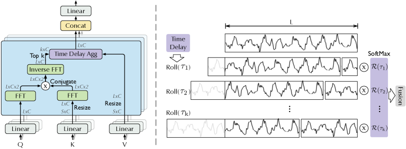
Figure 2: Auto-Correlation (left) and Time Delay Aggregation (right). We utilize the Fast Fourier Transform to calculate the autocorrelation $\mathcal{R}(\tau)$, which reflects the time-delay similarities. Then the similar sub-processes are rolled to the same index based on selected delay $\tau$ and aggregated by $\mathcal{R}(\tau)$.

3.2 Auto-Correlation Mechanism

As shown in Figure 2, we propose the Auto-Correlation mechanism with series-wise connections to expand the information utilization. Auto-Correlation discovers the period-based dependencies by calculating the series autocorrelation and aggregates similar sub-series by time delay aggregation.

Period-based dependencies

It is observed that the same phase position among periods naturally provides similar sub-processes.

Inspired by the stochastic process theory [9, 30], for a real discrete-time process $\{\mathcal{X}_{t}\}$, we can obtain the autocorrelation $\mathcal{R}_{\mathcal{X}\mathcal{X}}(\tau)$ by the following equations:

$$\begin{split}\mathcal{R}_{\mathcal{X}\mathcal{X}}(\tau)=\lim_{L\to\infty}\frac{1}{L}\sum_{t=1}^{L}\mathcal{X}_{t}\mathcal{X}_{t-\tau}.\end{split}$$ (5)

$\mathcal{R}_{\mathcal{X}\mathcal{X}}(\tau)$ reflects the time-delay similarity between $\{\mathcal{X}_{t}\}$ and its $\tau$ lag series $\{\mathcal{X}_{t-\tau}\}$. As shown in Figure 2, we use the autocorrelation $\mathcal{R}(\tau)$ as the unnormalized confidence of estimated period length $\tau$. Then, we choose the most possible $k$ period lengths $\tau_{1},\cdots,\tau_{k}$. The period-based dependencies are derived by the above estimated periods and can be weighted by the corresponding autocorrelation.

Time delay aggregation

The period-based dependencies connect the sub-series among estimated periods. Thus, we present the time delay aggregation block (Figure 2), which can roll the series based on selected time delay $\tau_{1},\cdots,\tau_{k}$. This operation can align similar sub-series that are at the same phase position of estimated periods, which is different from the point-wise dot-product aggregation in self-attention family. Finally, we aggregate the sub-series by softmax normalized confidences.

For the single head situation and time series $\mathcal{X}$ with length-$L$, after the projector, we get query $\mathcal{Q}$, key $\mathcal{K}$ and value $\mathcal{V}$. Thus, it can replace self-attention seamlessly. The Auto-Correlation mechanism is:

$$\begin{split}\tau_{1},\cdots,\tau_{k}&=\mathop{\arg\mathrm{Topk}}_{\tau\in\{1,\cdots,L\}}\left(\mathcal{R}_{\mathcal{Q},\mathcal{K}}(\tau)\right)\\ \widehat{\mathcal{R}}_{\mathcal{Q},\mathcal{K}}(\tau_{1}),\cdots,\widehat{\mathcal{R}}_{\mathcal{Q},\mathcal{K}}(\tau_{k})&=\mathrm{SoftMax}\left(\mathcal{R}_{\mathcal{Q},\mathcal{K}}(\tau_{1}),\cdots,\mathcal{R}_{\mathcal{Q},\mathcal{K}}(\tau_{k})\right)\\ \mathrm{Auto\text{-}Correlation}(\mathcal{Q},\mathcal{K},\mathcal{V})&=\sum_{i=1}^{k}\mathrm{Roll}(\mathcal{V},\tau_{i})\widehat{\mathcal{R}}_{\mathcal{Q},\mathcal{K}}(\tau_{i}),\end{split}$$ (6)

where $\arg\mathrm{Topk}(\cdot)$ is to get the arguments of the $\mathrm{Topk}$ autocorrelations and let $k=\lfloor c\times\log L\rfloor$, $c$ is a hyper-parameter. $\mathcal{R}_{\mathcal{Q},\mathcal{K}}$ is autocorrelation between series $\mathcal{Q}$ and $\mathcal{K}$. $\mathrm{Roll}(\mathcal{X},\tau)$ represents the operation to $\mathcal{X}$ with time delay $\tau$, during which elements that are shifted beyond the first position are re-introduced at the last position. For the encoder-decoder Auto-Correlation (Figure 1), $\mathcal{K},\mathcal{V}$ are from the encoder $\mathcal{X}_{\mathrm{en}}^{N}$ and will be resized to length-$O$, $\mathcal{Q}$ is from the previous block of the decoder.

For the multi-head version used in Autoformer, with hidden variables of $d_{\mathrm{model}}$ channels, $h$ heads, the query, key and value for $i$-th head are $\mathcal{Q}_{i},\mathcal{K}_{i},\mathcal{V}_{i}\in\mathbb{R}^{L\times\frac{d_{\mathrm{model}}}{h}},i\in\{1,\cdots,h\}$. The process is:

$$\begin{split}\mathrm{MultiHead}(\mathcal{Q},\mathcal{K},\mathcal{V})&=\mathcal{W_{\mathrm{output}}}\ast\mathrm{Concat}(\mathrm{head}_{1},\cdots,\mathrm{head}_{h})\\ \mathrm{where}\ \mathrm{head}_{i}&=\mathrm{Auto\text{-}Correlation}(\mathcal{Q}_{i},\mathcal{K}_{i},\mathcal{V}_{i}).\end{split}$$ (7)

Efficient computation

For period-based dependencies, these dependencies point to sub-processes at the same phase position of underlying periods and are inherently sparse. Here, we select the most possible delays to avoid picking the opposite phases. Because we aggregate $\mathcal{O}(\log L)$ series whose length is $L$, the complexity of Equations 6 and 7 is $\mathcal{O}(L\log L)$. For the autocorrelation computation (Equation 5), given time series $\{\mathcal{X}_{t}\}$, $\mathcal{R}_{\mathcal{X}\mathcal{X}}(\tau)$ can be calculated by Fast Fourier Transforms (FFT) based on the Wiener–Khinchin theorem [43]:

$$\begin{split}\mathcal{S}_{\mathcal{X}\mathcal{X}}(f)&=\mathcal{F}\left(\mathcal{X}_{t}\right)\mathcal{F}^{\ast}\left(\mathcal{X}_{t}\right)=\int_{-\infty}^{\infty}\mathcal{X}_{t}e^{-i2\pi tf}{\rm d}t\overline{\int_{-\infty}^{\infty}\mathcal{X}_{t}e^{-i2\pi tf}{\rm d}t}\\ \mathcal{R}_{\mathcal{X}\mathcal{X}}(\tau)&=\mathcal{F}^{-1}\left(\mathcal{S}_{\mathcal{X}\mathcal{X}}(f)\right)=\int_{-\infty}^{\infty}\mathcal{S}_{\mathcal{X}\mathcal{X}}(f)e^{i2\pi f\tau}{\rm d}f,\\ \end{split}$$ (8)

where $\tau\in\{1,\cdots,L\}$, $\mathcal{F}$ denotes the FFT and $\mathcal{F}^{-1}$ is its inverse. $\ast$ denotes the conjugate operation and $\mathcal{S}_{\mathcal{X}\mathcal{X}}(f)$ is in the frequency domain. Note that the series autocorrelation of all lags in $\{1,\cdots,L\}$ can be calculated at once by FFT. Thus, Auto-Correlation achieves the $\mathcal{O}(L\log L)$ complexity.

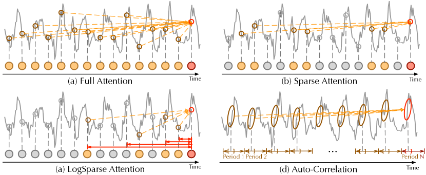
Figure 3: Auto-Correlation vs. self-attention family. Full Attention [41] (a) adapts the fully connection among all time points. Sparse Attention [23, 48] (b) selects points based on the proposed similarity metrics. LogSparse Attention [26] (c) chooses points following the exponentially increasing intervals. Auto-Correlation (d) focuses on the connections of sub-series among underlying periods.

Auto-Correlation vs. self-attention family

Different from the point-wise self-attention family, Auto-Correlation presents the series-wise connections (Figure 3). Concretely, for the temporal dependencies, we find the dependencies among sub-series based on the periodicity. In contrast, the self-attention family only calculates the relation between scattered points. Though some self-attentions [26, 48] consider the local information, they only utilize this to help point-wise dependencies discovery. For the information aggregation, we adopt the time delay block to aggregate the similar sub-series from underlying periods. In contrast, self-attentions aggregate the selected points by dot-product. Benefiting from the inherent sparsity and sub-series-level representation aggregation, Auto-Correlation can simultaneously benefit the computation efficiency and information utilization.

4 Experiments

We extensively evaluate the proposed Autoformer on six real-world benchmarks, covering five mainstream time series forecasting applications: energy, traffic, economics, weather and disease.

Datasets

Here is a description of the six experiment datasets: (1) ETT [48] dataset contains the data collected from electricity transformers, including load and oil temperature that are recorded every 15 minutes between July 2016 and July 2018. (2) Electricity dataset contains the hourly electricity consumption of 321 customers from 2012 to 2014. (3) Exchange [25] records the daily exchange rates of eight different countries ranging from 1990 to 2016. (4) Traffic is a collection of hourly data from California Department of Transportation, which describes the road occupancy rates measured by different sensors on San Francisco Bay area freeways. (5) Weather is recorded every 10 minutes for 2020 whole year, which contains 21 meteorological indicators, such as air temperature, humidity, etc. (6) ILI includes the weekly recorded influenza-like illness (ILI) patients data from Centers for Disease Control and Prevention of the United States between 2002 and 2021, which describes the ratio of patients seen with ILI and the total number of the patients. We follow standard protocol and split all datasets into training, validation and test set in chronological order by the ratio of 6:2:2 for the ETT dataset and 7:1:2 for the other datasets.

Table 1: Multivariate results with different prediction lengths $O\in\{96,192,336,720\}$. We set the input length $I$ as 36 for ILI and 96 for the others. A lower MSE or MAE indicates a better prediction.

Models		Autoformer		Informer[48]		LogTrans[26]		Reformer[23]		LSTNet[25]		LSTM[17]		TCN[4]
Metric		MSE	MAE	MSE	MAE	MSE	MAE	MSE	MAE	MSE	MAE	MSE	MAE	MSE	MAE
ETT∗	96	0.255	0.339	0.365	0.453	0.768	0.642	0.658	0.619	3.142	1.365	2.041	1.073	3.041	1.330
	192	0.281	0.340	0.533	0.563	0.989	0.757	1.078	0.827	3.154	1.369	2.249	1.112	3.072	1.339
	336	0.339	0.372	1.363	0.887	1.334	0.872	1.549	0.972	3.160	1.369	2.568	1.238	3.105	1.348
	720	0.422	0.419	3.379	1.388	3.048	1.328	2.631	1.242	3.171	1.368	2.720	1.287	3.135	1.354
Electricity	96	0.201	0.317	0.274	0.368	0.258	0.357	0.312	0.402	0.680	0.645	0.375	0.437	0.985	0.813
	192	0.222	0.334	0.296	0.386	0.266	0.368	0.348	0.433	0.725	0.676	0.442	0.473	0.996	0.821
	336	0.231	0.338	0.300	0.394	0.280	0.380	0.350	0.433	0.828	0.727	0.439	0.473	1.000	0.824
	720	0.254	0.361	0.373	0.439	0.283	0.376	0.340	0.420	0.957	0.811	0.980	0.814	1.438	0.784
Exchange	96	0.197	0.323	0.847	0.752	0.968	0.812	1.065	0.829	1.551	1.058	1.453	1.049	3.004	1.432
	192	0.300	0.369	1.204	0.895	1.040	0.851	1.188	0.906	1.477	1.028	1.846	1.179	3.048	1.444
	336	0.509	0.524	1.672	1.036	1.659	1.081	1.357	0.976	1.507	1.031	2.136	1.231	3.113	1.459
	720	1.447	0.941	2.478	1.310	1.941	1.127	1.510	1.016	2.285	1.243	2.984	1.427	3.150	1.458
Traffic	96	0.613	0.388	0.719	0.391	0.684	0.384	0.732	0.423	1.107	0.685	0.843	0.453	1.438	0.784
	192	0.616	0.382	0.696	0.379	0.685	0.390	0.733	0.420	1.157	0.706	0.847	0.453	1.463	0.794
	336	0.622	0.337	0.777	0.420	0.733	0.408	0.742	0.420	1.216	0.730	0.853	0.455	1.479	0.799
	720	0.660	0.408	0.864	0.472	0.717	0.396	0.755	0.423	1.481	0.805	1.500	0.805	1.499	0.804
Weather	96	0.266	0.336	0.300	0.384	0.458	0.490	0.689	0.596	0.594	0.587	0.369	0.406	0.615	0.589
	192	0.307	0.367	0.598	0.544	0.658	0.589	0.752	0.638	0.560	0.565	0.416	0.435	0.629	0.600
	336	0.359	0.395	0.578	0.523	0.797	0.652	0.639	0.596	0.597	0.587	0.455	0.454	0.639	0.608
	720	0.419	0.428	1.059	0.741	0.869	0.675	1.130	0.792	0.618	0.599	0.535	0.520	0.639	0.610
ILI	24	3.483	1.287	5.764	1.677	4.480	1.444	4.400	1.382	6.026	1.770	5.914	1.734	6.624	1.830
	36	3.103	1.148	4.755	1.467	4.799	1.467	4.783	1.448	5.340	1.668	6.631	1.845	6.858	1.879
	48	2.669	1.085	4.763	1.469	4.800	1.468	4.832	1.465	6.080	1.787	6.736	1.857	6.968	1.892
	60	2.770	1.125	5.264	1.564	5.278	1.560	4.882	1.483	5.548	1.720	6.870	1.879	7.127	1.918

• ETT means the ETTm2. See Appendix A for the full benchmark of ETTh1, ETTh2, ETTm1.

Implementation details

Our method is trained with the L2 loss, using the ADAM [22] optimizer with an initial learning rate of $10^{-4}$. Batch size is set to 32. The training process is early stopped within 10 epochs. All experiments are repeated three times, implemented in PyTorch [31] and conducted on a single NVIDIA TITAN RTX 24GB GPUs. The hyper-parameter $c$ of Auto-Correlation is in the range of 1 to 3 to trade off performance and efficiency. See Appendix E and B for standard deviations and sensitivity analysis. Autoformer contains 2 encoder layers and 1 decoder layer.

Baselines

We include 10 baseline methods. For the multivariate setting, we select three latest state-of-the-art transformer-based models: Informer [48], Reformer [23], LogTrans [26], two RNN-based models: LSTNet [25], LSTM [17] and CNN-based TCN [4] as baselines. For the univariate setting, we include more competitive baselines: N-BEATS[29], DeepAR [34], Prophet [39] and ARMIA [1].

4.1 Main Results

To compare performances under different future horizons, we fix the input length and evaluate models with a wide range of prediction lengths: 96, 192, 336, 720. This setting precisely meets the definition of long-term forecasting. Here are results on both the multivariate and univariate settings.

Multivariate results

As for the multivariate setting, Autoformer achieves the consistent state-of-the-art performance in all benchmarks and all prediction length settings (Table 10). Especially, under the input-96-predict-336 setting, compared to previous state-of-the-art results, Autoformer gives 74% (1.334$\to$0.339) MSE reduction in ETT, 18% (0.280$\to$0.231) in Electricity, 61% (1.357$\to$0.509) in Exchange, 15% (0.733$\to$0.622) in Traffic and 21% (0.455$\to$0.359) in Weather. For the input-36-predict-60 setting of ILI, Autoformer makes 43% (4.882$\to$2.770) MSE reduction. Overall, Autoformer yields a 38% averaged MSE reduction among above settings. Note that Autoformer still provides remarkable improvements in the Exchange dataset that is without obvious periodicity. See Appendix E for detailed showcases. Besides, we can also find that the performance of Autoformer changes quite steadily as the prediction length $O$ increases. It means that Autoformer retains better long-term robustness, which is meaningful for real-world practical applications, such as weather early warning and long-term energy consumption planning.

Univariate results

We list the univariate results of two typical datasets in Table 2. Under the comparison with extensive baselines, our Autoformer still achieves state-of-the-art performance for the long-term forecasting tasks. In particular, for the input-96-predict-336 setting, our model achieves 14% (0.180$\to$0.145) MSE reduction on the ETT dataset with obvious periodicity. For the Exchange dataset without obvious periodicity, Autoformer surpasses other baselines by 17% (0.611$\to$0.508) and shows greater long-term forecasting capacity. Also, we find that ARIMA [1] performs best in the input-96-predict-96 setting of the Exchange dataset but fails in the long-term setting. This situation of ARIMA can be benefited from its inherent capacity for non-stationary economic data but is limited by the intricate temporal patterns of real-world series.

Table 2: Univariate results with different prediction lengths $O\in\{96,192,336,720\}$ on typical datasets. We set the input length $I$ as 96. A lower MSE or MAE indicates a better prediction.

Models		Autoformer		N-BEATS[29]		Informer[48]		LogTrans[26]		Reformer[23]		DeepAR[34]		Prophet[39]		ARIMA[1]
Metric		MSE	MAE	MSE	MAE	MSE	MAE	MSE	MAE	MSE	MAE	MSE	MAE	MSE	MAE	MSE	MAE
ETT	96	0.065	0.189	0.082	0.219	0.088	0.225	0.082	0.217	0.131	0.288	0.099	0.237	0.287	0.456	0.211	0.362
	192	0.118	0.256	0.120	0.268	0.132	0.283	0.133	0.284	0.186	0.354	0.154	0.310	0.312	0.483	0.261	0.406
	336	0.154	0.305	0.226	0.370	0.180	0.336	0.201	0.361	0.220	0.381	0.277	0.428	0.331	0.474	0.317	0.448
	720	0.182	0.335	0.188	0.338	0.300	0.435	0.268	0.407	0.267	0.430	0.332	0.468	0.534	0.593	0.366	0.487
Exchange	96	0.241	0.387	0.156	0.299	0.591	0.615	0.279	0.441	1.327	0.944	0.417	0.515	0.828	0.762	0.112	0.245
	192	0.273	0.403	0.669	0.665	1.183	0.912	1.950	1.048	1.258	0.924	0.813	0.735	0.909	0.974	0.304	0.404
	336	0.508	0.539	0.611	0.605	1.367	0.984	2.438	1.262	2.179	1.296	1.331	0.962	1.304	0.988	0.736	0.598
	720	0.991	0.768	1.111	0.860	1.872	1.072	2.010	1.247	1.280	0.953	1.894	1.181	3.238	1.566	1.871	0.935

4.2 Ablation studies

Table 3: Ablation of decomposition in multivariate ETT with MSE metric. Ours adopts our progressive architecture into other models. Sep employs two models to forecast pre-decomposed seasonal and trend-cyclical components separately. Promotion is the MSE reduction compared to Origin.

Input-96	Transformer[41]			Informer[48]			LogTrans[23]			Reformer[26]			Promotion
Predict-$O$	Origin	Sep	Ours	Origin	Sep	Ours	Origin	Sep	Ours	Origin	Sep	Ours	Sep	Ours
96	0.604	0.311	0.204	0.365	0.490	0.354	0.768	0.862	0.231	0.658	0.445	0.218	0.069	0.347
192	1.060	0.760	0.266	0.533	0.658	0.432	0.989	0.533	0.378	1.078	0.510	0.336	0.300	0.562
336	1.413	0.665	0.375	1.363	1.469	0.481	1.334	0.762	0.362	1.549	1.028	0.366	0.434	1.019
720	2.672	3.200	0.537	3.379	2.766	0.822	3.048	2.601	0.539	2.631	2.845	0.502	0.079	2.332

Decomposition architecture

With our proposed progressive decomposition architecture, other models can gain consistent promotion, especially as the prediction length $O$ increases (Table 3). This verifies that our method can generalize to other models and release the capacity of other dependencies learning mechanisms, alleviate the distraction caused by intricate patterns. Besides, our architecture outperforms the pre-processing, although the latter employs a bigger model and more parameters. Especially, pre-decomposing may even bring negative effect because it neglects the interaction of components during long-term future, such as Transformer [41] predict-720, Informer [48] predict-336.

Auto-Correlation vs. self-attention family

As shown in Table 4, our proposed Auto-Correlation achieves the best performance under various input-$I$-predict-$O$ settings, which verifies the effectiveness of series-wise connections comparing to point-wise self-attentions (Figure 3). Furthermore, we can also observe that Auto-Correlation is memory efficiency from the last column of Table 4, which can be used in long sequence forecasting, such as input-336-predict-1440.

Table 4: Comparison of Auto-Correlation and self-attention in the multivariate ETT. We replace the Auto-Correlation in Autoformer with different self-attentions. The “-” indicates the out-of-memory.

Input Length $I$		96			192			336
Prediction Length $O$		336	720	1440	336	720	1440	336	720	1440
Auto-	MSE	0.339	0.422	0.555	0.355	0.429	0.503	0.361	0.425	0.574
Correlation	MAE	0.372	0.419	0.496	0.392	0.430	0.484	0.406	0.440	0.534
Full	MSE	0.375	0.537	0.667	0.450	0.554	-	0.501	0.647	-
Attention[41]	MAE	0.425	0.502	0.589	0.470	0.533	-	0.485	0.491	-
LogSparse	MSE	0.362	0.539	0.582	0.420	0.552	0.958	0.474	0.601	-
Attention[26]	MAE	0.413	0.522	0.529	0.450	0.513	0.736	0.474	0.524	-
LSH	MSE	0.366	0.502	0.663	0.407	0.636	1.069	0.442	0.615	-
Attention[23]	MAE	0.404	0.475	0.567	0.421	0.571	0.756	0.476	0.532	-
ProbSparse	MSE	0.481	0.822	0.715	0.404	1.148	0.732	0.417	0.631	1.133
Attention[48]	MAE	0.472	0.559	0.586	0.425	0.654	0.602	0.434	0.528	0.691

4.3 Model Analysis

Time series decomposition

As shown in Figure 4, without our series decomposition block, the forecasting model cannot capture the increasing trend and peaks of the seasonal part. By adding the series decomposition blocks, Autoformer can aggregate and refine the trend-cyclical part from series progressively. This design also facilitates the learning of the seasonal part, especially the peaks and troughs. This verifies the necessity of our proposed progressive decomposition architecture.

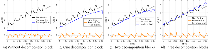
Figure 4: Visualization of learned seasonal $\mathcal{X}_{\mathrm{de}}^{M}$ and trend-cyclical $\mathcal{T}_{\mathrm{de}}^{M}$ of the last decoder layer. We gradually add the decomposition blocks in decoder from left to right. This case is from ETT dataset under input-96-predict-720 setting. For clearness, we add the linear growth to raw data additionally.

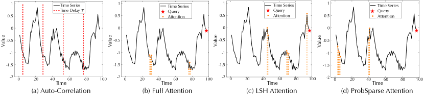
Figure 5: Visualization of learned dependencies. For clearness, we select the top-6 time delay sizes $\tau_{1},\cdots,\tau_{6}$ of Auto-Correlation and mark them in raw series (red lines). For self-attentions, top-6 similar points with respect to the last time step (red stars) are also marked by orange points.

Dependencies learning

The marked time delay sizes in Figure 5(a) indicate the most likely periods. Our learned periodicity can guide the model to aggregate the sub-series from the same or neighbor phase of periods by $\mathrm{Roll}(\mathcal{X},\tau_{i}),\ i\in\{1,\cdots,6\}$. For the last time step (declining stage), Auto-Correlation fully utilizes all similar sub-series without omissions or errors compared to self-attentions. This verifies that Autoformer can discover the relevant information more sufficiently and precisely.

Complex seasonality modeling

As shown in Figure 6, the lags that Autoformer learns from deep representations can indicate the real seasonality of raw series. For example, the learned lags of the daily recorded Exchange dataset present the monthly, quarterly and yearly periods (Figure 6 (b)). For the hourly recorded Traffic dataset (Figure 6 (c)), the learned lags show the intervals as 24-hours and 168-hours, which match the daily and weekly periods of real-world scenarios. These results show that Autoformer can capture the complex seasonalities of real-world series from deep representations and further provide a human-interpretable prediction.

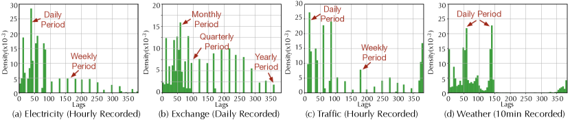
Figure 6: Statistics of learned lags. For each time series in the test set, we count the top 10 lags learned by decoder for the input-96-predict-336 task. Figure (a)-(d) are the density histograms.

Efficiency analysis

We compare the running memory and time among Auto-Correlation-based and self-attention-based models (Figure 7) during the training phase. The proposed Autoformer shows $\mathcal{O}(L\log L)$ complexity in both memory and time and achieves better long-term sequences efficiency.

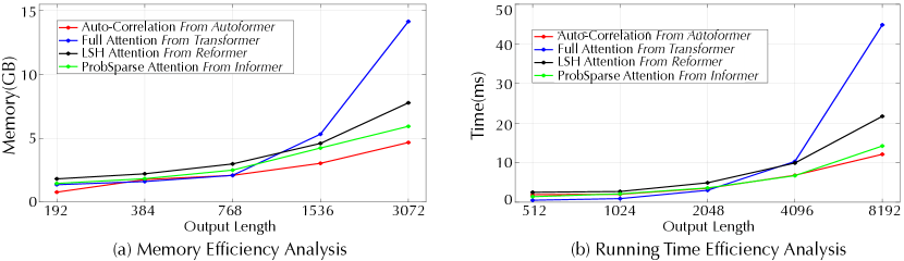
Figure 7: Efficiency Analysis. For memory, we replace Auto-Correlation with self-attention family in Autoformer and record the memory with input 96. For running time, we run the Auto-Correlation or self-attentions $10^{3}$ times to get the execution time per step. The output length increases exponentially.

5 Conclusions

This paper studies the long-term forecasting problem of time series, which is a pressing demand for real-world applications. However, the intricate temporal patterns prevent the model from learning reliable dependencies. We propose the Autoformer as a decomposition architecture by embedding the series decomposition block as an inner operator, which can progressively aggregate the long-term trend part from intermediate prediction. Besides, we design an efficient Auto-Correlation mechanism to conduct dependencies discovery and information aggregation at the series level, which contrasts clearly from the previous self-attention family. Autoformer can naturally achieve $\mathcal{O}(L\log L)$ complexity and yield consistent state-of-the-art performance in extensive real-world datasets.

Appendix A Full Benchmark on the ETT Datasets

As shown in Table 5, we build the benchmark on the four ETT datasets [48], which includes the hourly recorded ETTh1 and ETTh2, 15-minutely recorded ETTm1 and ETTm2.

Autoformer achieves sharp improvement over the state-of-the-art on various forecasting horizons. For the input-96-predict-336 long-term setting, Autoformer surpasses previous best results by 55% (1.128$\to$0.505) in ETTh1, 80% (2.544$\to$0.471) in ETTh2. For the input-96-predict-288 long-term setting, Autoformer achieves 40% (1.056$\to$0.634) MSE reduction in ETTm1 and 66% (0.969$\to$0.342) in ETTm2. These results show a 60% average MSE reduction over previous state-of-the-art.

Table 5: Multivariate results on the four ETT datasets with predicted length as {24, 48, 168, 288, 336, 672, 720}. We fix the input length of Autoformer as 96. The experiments of the main text are on the ETTm2 dataset.

Models		Autoformer		Informer [48]		LogTrans [26]		Reformer [23]		LSTNet [25]		LSTMa [3]
Metric		MSE	MAE	MSE	MAE	MSE	MAE	MSE	MAE	MSE	MAE	MSE	MAE
ETTh1	24	0.384	0.425	0.577	0.549	0.686	0.604	0.991	0.754	1.293	0.901	0.650	0.624
	48	0.392	0.419	0.685	0.625	0.766	0.757	1.313	0.906	1.456	0.960	0.702	0.675
	168	0.490	0.481	0.931	0.752	1.002	0.846	1.824	1.138	1.997	1.214	1.212	0.867
	336	0.505	0.484	1.128	0.873	1.362	0.952	2.117	1.280	2.655	1.369	1.424	0.994
	720	0.498	0.500	1.215	0.896	1.397	1.291	2.415	1.520	2.143	1.380	1.960	1.322
ETTh2	24	0.261	0.341	0.720	0.665	0.828	0.750	1.531	1.613	2.742	1.457	1.143	0.813
	48	0.312	0.373	1.457	1.001	1.806	1.034	1.871	1.735	3.567	1.687	1.671	1.221
	168	0.457	0.455	3.489	1.515	4.070	1.681	4.660	1.846	3.242	2.513	4.117	1.674
	336	0.471	0.475	2.723	1.340	3.875	1.763	4.028	1.688	2.544	2.591	3.434	1.549
	720	0.474	0.484	3.467	1.473	3.913	1.552	5.381	2.015	4.625	3.709	3.963	1.788
ETTm1	24	0.383	0.403	0.323	0.369	0.419	0.412	0.724	0.607	1.968	1.170	0.621	0.629
	48	0.454	0.453	0.494	0.503	0.507	0.583	1.098	0.777	1.999	1.215	1.392	0.939
	96	0.481	0.463	0.678	0.614	0.768	0.792	1.433	0.945	2.762	1.542	1.339	0.913
	288	0.634	0.528	1.056	0.786	1.462	1.320	1.820	1.094	1.257	2.076	1.740	1.124
	672	0.606	0.542	1.192	0.926	1.669	1.461	2.187	1.232	1.917	2.941	2.736	1.555
ETTm2	24	0.153	0.261	0.173	0.301	0.211	0.332	0.333	0.429	1.101	0.831	0.580	0.572
	48	0.178	0.280	0.303	0.409	0.427	0.487	0.558	0.571	2.619	1.393	0.747	0.630
	96	0.255	0.339	0.365	0.453	0.768	0.642	0.658	0.619	3.142	1.365	2.041	1.073
	288	0.342	0.378	1.047	0.804	1.090	0.806	2.441	1.190	2.856	1.329	0.969	0.742
	672	0.434	0.430	3.126	1.302	2.397	1.214	3.090	1.328	3.409	1.420	2.541	1.239

Appendix B Hyper-Parameter Sensitivity

As shown in Table 6, we can verify the model robustness with respect to hyper-parameter $c$ (Equation 6 in the main text). To trade-off performance and efficiency, we set $c$ to the range of 1 to 3. It is also observed that datasets with obvious periodicity tend to have a large factor $c$, such as the ETT and Traffic datasets. For the ILI dataset without obvious periodicity, the larger factor may bring noises.

Table 6: Autoformer performance under different choices of hyper-parameter $c$ in the Auto-Correlation mechanism. We adopt the forecasting setting as input-36-predict-48 for the ILI dataset and input-96-predict-336 for the other datasets.

Dataset	ETT		Electricity		Exchange		Traffic		Weather		ILI
Metric	MSE	MAE	MSE	MAE	MSE	MAE	MSE	MAE	MSE	MAE	MSE	MAE
$c=1$	0.339	0.372	0.252	0.356	0.511	0.528	0.706	0.488	0.348	0.388	2.754	1.088
$c=2$	0.363	0.389	0.224	0.332	0.511	0.528	0.673	0.418	0.358	0.390	2.641	1.072
$c=3$	0.339	0.372	0.231	0.338	0.509	0.524	0.619	0.385	0.359	0.395	2.669	1.085
$c=4$	0.336	0.369	0.232	0.341	0.513	0.527	0.607	0.378	0.349	0.388	3.041	1.178
$c=5$	0.410	0.415	0.273	0.371	0.517	0.527	0.618	0.379	0.366	0.399	3.076	1.172

Appendix C Model Input Selection

C.1 Input Length Selection

Because the forecasting horizon is always fixed upon the application’s demand, we need to tune the input length in real-world applications. Our study shows that the relationship between input length and model performance is dataset-specific, so we need to select the model input based on the data characteristics. For example, for the ETT dataset with obvious periodicity, an input with length-96 is enough to provide enough information. But for the ILI dataset without obvious periodicity, the model needs longer inputs to discover more informative temporal dependencies. Thus, a longer input will provide a better performance in the ILI dataset.

Table 7: Autoformer performance under different input lengths. We fix the forecasting horizon as 48 for ILI and 336 for the others. The input lengths $I$ of the ILI dataset are in the {24, 36, 48, 60}. And for the ETT and Exchange datasets, the input lengths $I$ are in the {96, 192, 336, 720}.

Dataset	ETT		Electricity		Dataset	ILI
Metric	MSE	MAE	MSE	MAE	Metric	MSE	MAE
$I=96$	0.339	0.372	0.231	0.338	$I=24$	3.406	1.247
$I=192$	0.355	0.392	0.200	0.316	$I=36$	2.669	1.085
$I=336$	0.361	0.406	0.225	0.335	$I=48$	2.656	1.075
$I=720$	0.419	0.430	0.226	0.346	$I=60$	2.779	1.091

C.2 Past Information Utilization

For the decoder input of Autoformer, we attach the length-$\frac{I}{2}$ past information to the placeholder. This design is to provide recent past information to the decoder. As shown in Table 8, the model with more past information will obtain a better performance, but it also causes a larger memory cost. Thus, we set the decoder input as $\frac{I}{2}+O$ to trade off both the performance and efficiency.

Table 8: Autoformer performance under different lengths of input of the decoder. $O$, $\frac{I}{2}+O$, $I+O$ corresponds to the decoder input without past information, with half past information, with full past information respectively. We fix the forecasting setting as input-96-predict-336 on the ETT dataset.

Decoder input length	$O$ (without past)	$\frac{I}{2}+O$ (with half past)	$I+O$ (with full past)
MSE	0.360	0.339	0.333
MAE	0.383	0.372	0.369
Memory Cost	3029 MB	3271 MB	3599 MB

Appendix D Ablation of Decomposition Architecture

In this section, we attempt to further verify the effectiveness of our proposed progressive decomposition architecture. We adopt more well-established decomposition algorithms as the pre-processing for separate prediction settings. As shown in Table 9, our proposed progressive decomposition architecture consistently outperforms the separate prediction (especially the long-term forecasting setting), despite the latter being with mature decomposition algorithms and twice bigger model.

Table 9: Ablation of decomposition architecture in ETT dataset under the input-96-predict-$O$ setting, where $O\in\{96,192,336,720\}$. The backbone of separate prediction is canonical Transformer [41]. We adopt various decomposition algorithms as the pre-processing and use two Transformers to separately forecast the seasonal and trend-cyclical parts. The result is the sum of two parts prediction.

Decomposition	Predict $O$	96		192		336		720
	Metric	MSE	MAE	MSE	MAE	MSE	MAE	MSE	MAE
Separately	STL [33]	0.523	0.516	0.638	0.605	1.004	0.794	3.678	1.462
	Hodrick-Prescott Filter [18]	0.464	0.495	0.816	0.733	0.814	0.722	2.181	1.173
	Christiano-Fitzgerald Filter [11]	0.373	0.458	0.819	0.668	1.083	0.835	2.462	1.189
	Baxter-King Filter [44]	0.440	0.514	0.623	0.626	0.861	0.741	2.150	1.175
Progressively	Autoformer	0.255	0.339	0.281	0.340	0.339	0.372	0.422	0.419

Appendix E Supplementary of Main Results

E.1 Multivariate Showcases

To evaluate the prediction of different models, we plot the last dimension of forecasting results that are from the test set of ETT dataset for qualitative comparison (Figures 8, 9, 10, and 11). Our model gives the best performance among different models. Moreover, we observe that Autoformer can accurately predict the periodicity and long-term variation.

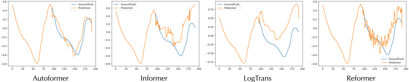
Figure 8: Prediction cases from the ETT dataset under the input-96-predict-96 setting. Blue lines are the ground truth and orange lines are the model prediction. The first part with length 96 is the input.

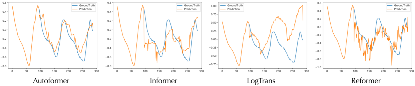
Figure 9: Prediction cases from the ETT dataset under the input-96-predict-192 setting.

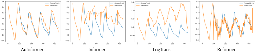
Figure 10: Prediction cases from the ETT dataset under the input-96-predict-336 setting.

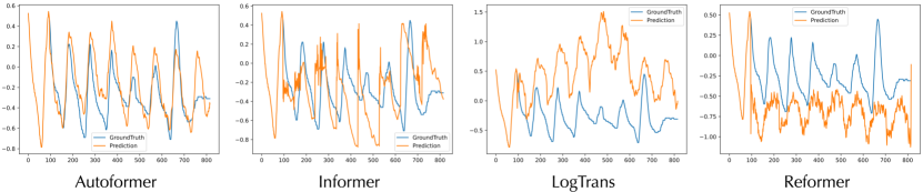
Figure 11: Prediction cases from the ETT dataset under the input-96-predict-720 setting.

E.2 Performance on Data without Obvious Periodicity

Autoformer yields the best performance among six datasets, even in the Exchange dataset that does not have obvious periodicity. This section will give some showcases from the test set of multivariate Exchange dataset for qualitative evaluation. We observed that the series in the Exchange dataset show rapid fluctuations. And because of the inherent properties of economic data, the series does not present obvious periodicity. This aperiodicity causes extreme difficulties for prediction. As shown in Figure 12, compared to other models, Autoformer can still predict the exact long-term variations. It is verified the robustness of our model performance among various data characteristics.

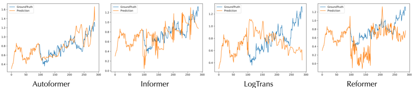
Figure 12: Prediction cases from the Exchange dataset under the input-96-predict-192 setting.

E.3 Univariate Forecasting Showcases

As shown in Figure 13, Autoformer gives the most accurate prediction. Compared to Informer [48], Autoformer can precisely capture the periods of the future horizon. Besides, our model provides better prediction in the center area than LogTrans [26]. Compared with Reformer [23], our prediction series is smooth and closer to ground truth. Also, the fluctuation of DeepAR [34] prediction is getting smaller as prediction length increases and suffers from the over-smoothing problem, which does not happen in our Autoformer.

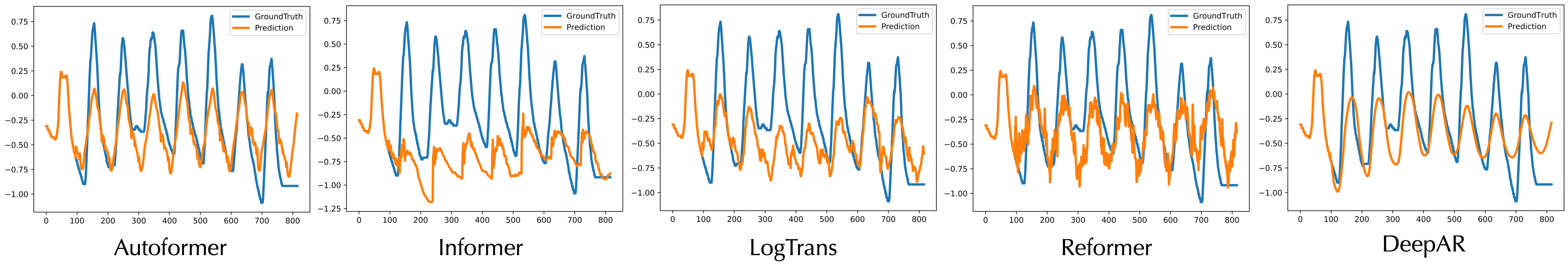
Figure 13: Prediction cases from the ETT dataset under the input-96-predict-720 univariate setting.

E.4 Main Results with Standard Deviations

To get more robust experimental results, we repeat each experiment three times. The results are shown without standard deviations in the main text due to the limited pages. Table 10 shows the standard deviations.

Table 10: Quantitative results with fluctuations under different prediction lengths $O$ for multivariate forecasting. We set the input length $I$ as 36 for ILI and 96 for the other datasets. A lower MSE or MAE indicates a better performance.

Models		Autoformer		Informer[48]		LogTrans[26]		Reformer[23]
Metric		MSE	MAE	MSE	MAE	MSE	MAE	MSE	MAE
ETT	96	0.255 $\pm$0.020	0.339 $\pm$0.020	0.365 $\pm$0.062	0.453 $\pm$0.047	0.768 $\pm$0.071	0.642 $\pm$0.020	0.658 $\pm$0.121	0.619 $\pm$0.021
	192	0.281 $\pm$0.027	0.340 $\pm$0.025	0.533 $\pm$0.109	0.563 $\pm$0.050	0.989 $\pm$0.124	0.757 $\pm$0.049	1.078 $\pm$0.106	0.827 $\pm$0.012
	336	0.339 $\pm$0.018	0.372 $\pm$0.015	1.363 $\pm$0.173	0.887 $\pm$0.056	1.334 $\pm$0.168	0.872 $\pm$0.054	1.549 $\pm$0.146	0.972 $\pm$0.015
	720	0.422 $\pm$0.015	0.419 $\pm$0.010	3.379 $\pm$0.143	1.388 $\pm$0.037	3.048 $\pm$0.140	1.328 $\pm$0.023	2.631 $\pm$0.126	1.242 $\pm$0.014
Electricity	96	0.201 $\pm$0.003	0.317 $\pm$0.004	0.274 $\pm$0.004	0.368 $\pm$0.003	0.258 $\pm$0.002	0.357 $\pm$0.002	0.312 $\pm$0.003	0.402 $\pm$0.004
	192	0.222 $\pm$0.003	0.334 $\pm$0.004	0.296 $\pm$0.009	0.386 $\pm$0.007	0.266 $\pm$0.005	0.368 $\pm$0.004	0.348 $\pm$0.004	0.433 $\pm$0.005
	336	0.231 $\pm$0.006	0.338 $\pm$0.004	0.300 $\pm$0.007	0.394 $\pm$0.004	0.280 $\pm$0.006	0.380 $\pm$0.001	0.350 $\pm$0.004	0.433 $\pm$0.003
	720	0.254 $\pm$0.007	0.361 $\pm$0.008	0.373 $\pm$0.034	0.439 $\pm$0.024	0.283 $\pm$0.003	0.376 $\pm$0.002	0.340 $\pm$0.002	0.420 $\pm$0.002
Exchange	96	0.197 $\pm$0.019	0.323 $\pm$0.012	0.847 $\pm$0.150	0.752 $\pm$0.060	0.968 $\pm$0.177	0.812 $\pm$0.027	1.065 $\pm$0.070	0.829 $\pm$0.013
	192	0.300 $\pm$0.020	0.369 $\pm$0.016	1.204 $\pm$0.149	0.895 $\pm$0.061	1.040 $\pm$0.232	0.851 $\pm$0.029	1.188 $\pm$0.041	0.906 $\pm$0.008
	336	0.509 $\pm$0.041	0.524 $\pm$0.016	1.672 $\pm$0.036	1.036 $\pm$0.014	1.659 $\pm$0.122	1.081 $\pm$0.015	1.357 $\pm$0.027	0.976 $\pm$0.010
	720	1.447 $\pm$0.084	0.941 $\pm$0.028	2.478 $\pm$0.198	1.310 $\pm$0.070	1.941 $\pm$0.327	1.127 $\pm$0.030	1.510 $\pm$0.071	1.016 $\pm$0.008
Traffic	96	0.613 $\pm$0.028	0.388 $\pm$0.012	0.719$\pm$0.015	0.391 $\pm$0.004	0.684 $\pm$0.041	0.384 $\pm$0.008	0.732 $\pm$0.027	0.423 $\pm$0.025
	192	0.616 $\pm$0.042	0.382 $\pm$0.020	0.696 $\pm$0.050	0.379 $\pm$0.023	0.685 $\pm$0.055	0.390 $\pm$0.021	0.733 $\pm$0.013	0.420 $\pm$0.011
	336	0.622 $\pm$0.016	0.337 $\pm$0.011	0.777 $\pm$0.009	0.420 $\pm$0.003	0.733 $\pm$0.069	0.408 $\pm$0.026	0.742 $\pm$0.012	0.420 $\pm$0.008
	720	0.660 $\pm$0.025	0.408 $\pm$0.015	0.864 $\pm$0.026	0.472 $\pm$0.015	0.717 $\pm$0.030	0.396 $\pm$0.010	0.755 $\pm$0.023	0.423 $\pm$0.014
Weather	96	0.266 $\pm$0.007	0.336 $\pm$0.006	0.300 $\pm$0.013	0.384 $\pm$0.013	0.458 $\pm$0.143	0.490 $\pm$0.038	0.689 $\pm$0.042	0.596 $\pm$0.019
	192	0.307 $\pm$0.024	0.367 $\pm$0.022	0.598 $\pm$0.045	0.544 $\pm$0.028	0.658 $\pm$0.151	0.589 $\pm$0.032	0.752 $\pm$0.048	0.638 $\pm$0.029
	336	0.359 $\pm$0.035	0.395 $\pm$0.031	0.578 $\pm$0.024	0.523 $\pm$0.016	0.797 $\pm$0.034	0.652 $\pm$0.019	0.639 $\pm$0.030	0.596 $\pm$0.021
	720	0.419 $\pm$0.017	0.428 $\pm$0.014	1.059 $\pm$0.096	0.741 $\pm$0.042	0.869 $\pm$0.045	0.675 $\pm$0.093	1.130 $\pm$0.084	0.792 $\pm$0.055
ILI	24	3.483 $\pm$0.107	1.287 $\pm$0.018	5.764 $\pm$0.354	1.677 $\pm$0.080	4.480 $\pm$0.313	1.444 $\pm$0.033	4.400 $\pm$0.117	1.382 $\pm$0.021
	36	3.103 $\pm$0.139	1.148 $\pm$0.025	4.755 $\pm$0.248	1.467 $\pm$0.067	4.799 $\pm$0.251	1.467 $\pm$0.023	4.783 $\pm$0.138	1.448 $\pm$0.023
	48	2.669 $\pm$0.151	1.085 $\pm$0.037	4.763 $\pm$0.295	1.469 $\pm$0.059	4.800 $\pm$0.233	1.468 $\pm$0.021	4.832 $\pm$0.122	1.465 $\pm$0.016
	60	2.770 $\pm$0.085	1.125 $\pm$0.019	5.264 $\pm$0.237	1.564 $\pm$0.044	5.278 $\pm$0.231	1.560 $\pm$0.014	4.882 $\pm$0.123	1.483 $\pm$0.016

Appendix F COVID-19: Case Study

We also apply our model to the COVID-19 real-world data [15]. This dataset contains the data collected from countries, including the number of confirmed deaths and recovered patients of COVID-19 recorded daily from January 22, 2020, to May 20, 2021. We select two anonymous countries in Europe for the experiments. The data is split into training, validation and test set in chronological order following the ratio of 7:1:2 and normalized. Note that this problem is quite challenging because the training data is limited.

F.1 Quantitative Results

We still follow the long-term forecasting task and let the model predict the next week, half month, full month respectively. The prediction lengths are 1, 2.1, 4.3 times the input length. As shown in Table 11, Autoformer still keeps the state-of-the-art accuracy under the limited data and short input situation.

Table 11: Quantitative results for COVID-19 data. We set the input length $I$ as 7, which means that the data in one week. The prediction length $O$ is in $\{7,15,30\}$, which represents a week, half a month, a month respectively. A lower MSE or MAE indicates a better prediction.

Models		Autoformer		Informer[48]		LogTrans[26]		Reformer[23]		Transformer[41]
Metric		MSE	MAE	MSE	MAE	MSE	MAE	MSE	MAE	MSE	MAE
Country 1	7	0.110	0.213	0.168	0.323	0.190	0.311	0.219	0.312	0.156	0.254
	15	0.168	0.264	0.443	0.482	0.229	0.361	0.276	0.403	0.289	0.382
	30	0.261	0.319	0.443	0.482	0.311	0.356	0.276	0.403	0.362	0.444
Country 2	7	1.747	0.891	1.806	0.969	1.834	1.013	2.403	1.071	1.798	0.955
	15	1.749	0.905	1.842	0.969	1.829	1.004	2.627	1.111	1.830	0.999
	30	1.749	0.903	2.087	1.116	2.147	1.106	3.316	1.267	2.190	1.172

F.2 Showcases

As shown in Figure 14, compared to other models, our Autoformer can accurately predict the peaks and troughs at the beginning and can almost predict the exact value in the long-term future. The forecasting of extreme values and long-term trends are essential to epidemic prevention and control.

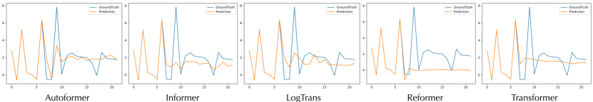
Figure 14: Showcases from the second country of COVID-19 under the input-7-predict-15 setting.

Appendix G Autoformer: Implementation Details

G.1 Model Design

We provide the pseudo-code of Autoformer and Auto-Correlation mechanism in Algorithms 1 and 2 respectively. The tensor shapes and hyper-parameter settings are also included. Besides the above standard version, we speed up the Auto-Correlation to a batch-normalization-style block for efficiency, namely speedup version. All the experiment results of this paper are from the speedup version. Here are the implementation details.

Speedup version

Note that the gather operation in Algorithm 2 is not memory-access friendly. We borrow the design of batch normalization [21] to speedup the Auto-Correlation mechanism. We separate the whole procedure as the training phase and the inference phase. Because of the property of the linear layer, the channels of deep representations are equivalent. Thus, we reduce the channel and head dimension for both the training and inference phases. Especially for the training phase, we average the autocorrelation within a batch to simplify the learned lags. This design speeds up Auto-Correlation and performs as normalization to obtain a global judgment of the learned lags because the series within a batch are samples from the same time-series dataset. The pseudo-code for the training phase is presented in Algorithm 3. For the testing phase, we still use the gather operation with respect to the simplified lags, which is more memory-access friendly than the standard version. The pseudo-code for the inference phase is presented in Algorithm 4.

Complexity analysis

Our model provides the series-wise aggregation for $\lfloor c\times\log L\rfloor$ delayed length-$L$ series. Thus, the complexity is $\mathcal{O}(L\log L)$ for both the standard version and the speedup version. However, the latter is faster because it is more memory-access friendly.

Algorithm 1 Overall Autoformer Procedure

1:Input past time series $\mathcal{X}$; Input Length $I$; Predict length $O$; Data dimension $d$; Hidden state channel $d_{\text{model}}$; Encoder layers number $N$; Decoder layers number $M$; Moving average window size $k$. Technically, we set $d_{\text{model}}$ as 512, $N$ as 2, $M$ as 1, $k$ as 25.

2:$\mathcal{X}_{\text{ens}},\mathcal{X}_{\text{ent}}=\texttt{SeriesDecomp}(\mathcal{X}_{\frac{I}{2}:I})$ $\triangleright$ $\mathcal{X}\in\mathbb{R}^{I\times d},\mathcal{X}_{\text{ens}},\mathcal{X}_{\text{ent}}\in\mathbb{R}^{\frac{I}{2}\times d}$

3:$\mathcal{X}_{0},\mathcal{X}_{\text{mean}}=\texttt{Zeros}([O,d]),\texttt{Repeat}\Big{(}\texttt{Mean}(\mathcal{X}_{\frac{I}{2}:I},\texttt{dim=0}),\texttt{dim=0}\Big{)}$ $\triangleright$ $\mathcal{X}_{0},\mathcal{X}_{\text{mean}}\in\mathbb{R}^{O\times d}$

4:$\mathcal{X}_{\text{des}},\mathcal{X}_{\text{det}}=\texttt{Concat}(\mathcal{X}_{\text{ens}},\mathcal{X}_{0}),\texttt{Concat}(\mathcal{X}_{\text{ent}},\mathcal{X}_{\text{mean}})$ $\triangleright$ $\mathcal{X}_{\text{des}},\mathcal{X}_{\text{det}}\in\mathbb{R}^{(\frac{I}{2}+O)\times d}$

5:$\mathcal{X}^{0}_{\text{en}}=\texttt{Embed}(\mathcal{X})$ $\triangleright$ $\mathcal{X}^{0}_{\text{en}}\in\mathbb{R}^{I\times d_{\text{model}}}$

6:$\textbf{for}\ l\ \textbf{in}\ \{1,\cdots,N\}\textbf{:}$$\triangleright$ Autoformer Encoder

7:$\textbf{{\color[rgb]{1,1,1}for}}\ \mathcal{S}_{\mathrm{en}}^{l,1},\underline{~{}~{}}=\texttt{SeriesDecomp}\Big{(}\texttt{Auto-Correlation}(\mathcal{X}_{\mathrm{en}}^{l-1})+\mathcal{X}_{\mathrm{en}}^{l-1}\Big{)}$$\triangleright$ $\mathcal{S}_{\mathrm{en}}^{l,1}\in\mathbb{R}^{I\times d_{\text{model}}}$

8:$\textbf{{\color[rgb]{1,1,1}for}}\ \mathcal{S}_{\mathrm{en}}^{l,2},\underline{~{}~{}}=\texttt{SeriesDecomp}\Big{(}\texttt{FeedForward}(\mathcal{S}_{\mathrm{en}}^{l,1})+\mathcal{S}_{\mathrm{en}}^{l,1}\Big{)}$$\triangleright$ $\mathcal{S}_{\mathrm{en}}^{l,2}\in\mathbb{R}^{I\times d_{\text{model}}}$

9:$\textbf{{\color[rgb]{1,1,1}for}}\ \mathcal{X}_{\text{en}}^{l}=\mathcal{S}_{\text{en}}^{l,2}$$\triangleright$ $\mathcal{X}_{\text{en}}^{l}\in\mathbb{R}^{I\times d_{\text{model}}}$

10:End for

11:$\mathcal{X}^{0}_{\text{de}}=\texttt{Embed}(\mathcal{X}_{\text{des}}),\ \mathcal{T}^{0}_{\text{de}}=\mathcal{X}_{\text{det}},$ $\triangleright$ $\mathcal{X}^{0}_{\text{de}}\in\mathbb{R}^{(\frac{I}{2}+O)\times d_{\text{model}}},\mathcal{T}^{0}_{\text{de}}\in\mathbb{R}^{(\frac{I}{2}+O)\times d}$

12:$\textbf{for}\ l\ \textbf{in}\ \{1,\cdots,M\}\textbf{:}$$\triangleright$ Autoformer Decoder

13:$\textbf{{\color[rgb]{1,1,1}for}}\ \mathcal{S}_{\mathrm{de}}^{l,1},\mathcal{T}_{\mathrm{de}}^{l,1}=\texttt{SeriesDecomp}\Big{(}\texttt{Auto-Correlation}(\mathcal{X}_{\mathrm{de}}^{l-1})+\mathcal{X}_{\mathrm{de}}^{l-1}\Big{)}$

14:$\textbf{{\color[rgb]{1,1,1}for}}\ \mathcal{S}_{\mathrm{de}}^{l,2},\mathcal{T}_{\mathrm{de}}^{l,2}=\texttt{SeriesDecomp}\Big{(}\texttt{Auto-Correlation}(\mathcal{S}_{\mathrm{de}}^{l,1},\mathcal{X}_{\mathrm{en}}^{N})+\mathcal{S}_{\mathrm{de}}^{l,1}\Big{)}$

15:$\textbf{{\color[rgb]{1,1,1}for}}\ \mathcal{S}_{\mathrm{de}}^{l,3},\mathcal{T}_{\mathrm{de}}^{l,3}=\texttt{SeriesDecomp}\Big{(}\texttt{FeedForward}(\mathcal{S}_{\mathrm{de}}^{l,2})+\mathcal{S}_{\mathrm{de}}^{l,2}\Big{)}$ $\triangleright$ $\mathcal{S}_{\mathrm{de}}^{l,\cdot},\mathcal{T}_{\mathrm{de}}^{l,\cdot}\in\mathbb{R}^{(\frac{I}{2}+O)\times d_{\text{model}}}$

16:$\textbf{{\color[rgb]{1,1,1}for}}\ \mathcal{T}_{\mathrm{de}}^{l}=\mathcal{T}_{\mathrm{de}}^{l-1}+\texttt{MLP}(\mathcal{T}_{\mathrm{de}}^{l,1})+\texttt{MLP}(\mathcal{T}_{\mathrm{de}}^{l,2})+\texttt{MLP}(\mathcal{T}_{\mathrm{de}}^{l,3})$ $\triangleright$ $\mathcal{T}_{\mathrm{de}}^{l}\in\mathbb{R}^{(\frac{I}{2}+O)\times d}$

17:$\textbf{{\color[rgb]{1,1,1}for}}\ \mathcal{X}_{\text{de}}^{l}=\mathcal{S}_{\text{de}}^{l,3}$$\triangleright$ $\mathcal{X}_{\text{de}}^{l}\in\mathbb{R}^{(\frac{I}{2}+O)\times d_{\text{model}}}$

18:End for

19:$\mathcal{X}_{\text{pred}}=\texttt{MLP}(\mathcal{X}_{\text{de}}^{M})+\mathcal{T}_{\mathrm{de}}^{M}$$\triangleright$ $\mathcal{X}_{\text{pred}}\in\mathbb{R}^{(\frac{I}{2}+O)\times d_{\text{model}}}$

20:$\textbf{Return}\ {\mathcal{X}_{\text{pred}}}_{\frac{I}{2}:\frac{I}{2}+O}$ $\triangleright$ Return the prediction results

Algorithm 2 Auto-Correlation (multi-head standard version for a batch of data)

1:Queries $\mathcal{Q}\in\mathbb{R}^{B\times L\times d_{\text{model}}}$; Keys $\mathcal{K}\in\mathbb{R}^{B\times S\times d_{\text{model}}}$; Values $\mathcal{V}\in\mathbb{R}^{B\times S\times d_{\text{model}}}$; Number of heads $h$; Hidden state channel $d_{\text{model}}$; Hyper-parameter $c$. We set $d_{\text{model}}$ as 512, $h$ as 8, $1\leq c\leq 3$.

2:$\mathcal{K},\mathcal{V}=\texttt{Resize}(\mathcal{K}),\texttt{Resize}(\mathcal{V})$ $\triangleright$ Resize is truncation or zero filling. $\mathcal{K},\mathcal{V}\in\mathbb{R}^{B\times L\times d_{\text{model}}}$

3:$\mathcal{Q},\mathcal{K},\mathcal{V}=\texttt{Reshape}(\mathcal{Q}),\texttt{Reshape}(\mathcal{K}),\texttt{Reshape}(\mathcal{V})$$\triangleright$ $\mathcal{Q},\mathcal{K},\mathcal{V}\in\mathcal{R}^{L\times h\times\frac{d_{\text{model}}}{h}}$

4:$\mathcal{Q}=\texttt{FFT}(\mathcal{Q},\texttt{dim=0}),\mathcal{K}=\texttt{FFT}(\mathcal{K},\texttt{dim=0}),$$\triangleright$ $\mathcal{Q},\mathcal{K}\in\mathbb{C}^{B\times L\times h\times\frac{d_{\text{model}}}{h}}$

5:$\text{Corr}=\texttt{IFFT}\Big{(}\mathcal{Q}\times\texttt{Conj}(\mathcal{K}),\texttt{dim=0}\Big{)}$$\triangleright$ Autocorrelation $\text{Corr}\in\mathbb{R}^{B\times L\times h\times\frac{d_{\text{model}}}{h}}$

6:$\text{W}_{\text{topk}},\text{I}_{\text{topk}}=\texttt{Topk}(\text{Corr},\lfloor c\times{\log L}\rfloor,\texttt{dim=0})$$\triangleright$ Largest weights $\text{W}_{\text{topk}}$ and their indices $\text{I}_{\text{topk}}$

7:$\text{W}_{\text{topk}}=\texttt{Softmax}(\text{W}_{\text{topk}},\texttt{dim=0})$$\triangleright$ $\text{W}_{\text{topk}},\text{I}_{\text{topk}}\in\mathbb{R}^{B\times(\lfloor c\times{\log L}\rfloor)\times h\times{\frac{d_{\text{model}}}{h}}}$

8:${\text{Index}}=\texttt{Repeat}\Big{(}\texttt{arange}(L)\Big{)}$$\triangleright$ Initialize series indices. $\text{Index}\in\mathbb{R}^{B\times L\times h\times\frac{d_{\text{model}}}{h}}$

9:$\mathcal{V}=\texttt{Repeat}(\mathcal{V})$$\triangleright$ $\mathcal{V}\in\mathbb{R}^{B\times(2L)\times h\times\frac{d_{\text{model}}}{h}}$

10:$\mathcal{R}=\Big{[}{\text{W}_{\text{topk}}}_{i,:,:}\times\texttt{gather}\Big{(}\mathcal{V},({\text{I}_{\text{topk}}}_{i,:,:}+\text{Index})\Big{)}\ \textbf{for}\ i\ \textbf{in}\ \texttt{range}(\lfloor c\times{\log L}\rfloor)\Big{]}$$\triangleright$ Aggregation

11:$\mathcal{R}=\texttt{Sum}\Big{(}\texttt{Stack}(\mathcal{R},\texttt{dim=0}),\texttt{dim=0}\Big{)}$$\triangleright$ $\mathcal{R}\in\mathbb{R}^{B\times L\times h\times\frac{d_{\text{model}}}{h}}$

12:$\textbf{Return}\ \mathcal{R}$ $\triangleright$ Return transformed results

Algorithm 3 Auto-Correlation (multi-head speedup version for the training phase)

1:Queries $\mathcal{Q}\in\mathbb{R}^{B\times L\times d_{\text{model}}}$; Keys $\mathcal{K}\in\mathbb{R}^{B\times S\times d_{\text{model}}}$; Values $\mathcal{V}\in\mathbb{R}^{B\times S\times d_{\text{model}}}$; Number of heads $h$; Hidden state channel $d_{\text{model}}$; Hyper-parameter $c$. We set $d_{\text{model}}$ as 512, $h$ as 8, $1\leq c\leq 3$.

2:$\mathcal{K},\mathcal{V}=\texttt{Resize}(\mathcal{K}),\texttt{Resize}(\mathcal{V})$ $\triangleright$ Resize is truncation or zero filling. $\mathcal{K},\mathcal{V}\in\mathbb{R}^{B\times L\times d_{\text{model}}}$

3:$\mathcal{Q},\mathcal{K},\mathcal{V}=\texttt{Reshape}(\mathcal{Q}),\texttt{Reshape}(\mathcal{K}),\texttt{Reshape}(\mathcal{V})$$\triangleright$ $\mathcal{Q},\mathcal{K},\mathcal{V}\in\mathcal{R}^{B\times L\times h\times\frac{d_{\text{model}}}{h}}$

4:$\mathcal{Q}=\texttt{FFT}(\mathcal{Q},\texttt{dim=0}),\mathcal{K}=\texttt{FFT}(\mathcal{K},\texttt{dim=0}),$$\triangleright$ $\mathcal{Q},\mathcal{K}\in\mathbb{C}^{B\times L\times h\times\frac{d_{\text{model}}}{h}}$

5:$\text{Corr}=\texttt{IFFT}\Big{(}\mathcal{Q}\times\texttt{Conj}(\mathcal{K}),\texttt{dim=0}\Big{)}$$\triangleright$ Autocorrelation $\text{Corr}\in\mathbb{R}^{B\times L\times h\times\frac{d_{\text{model}}}{h}}$

6:${\text{Corr}}=\texttt{Mean}(\text{Corr},dim=0,2,3)$$\triangleright$ Simplify lags. $\text{Corr}\in\mathbb{R}^{L}$

7:$\text{W}_{\text{topk}},\text{I}_{\text{topk}}=\texttt{Topk}(\text{Corr},\lfloor c\times{\log L}\rfloor,\texttt{dim=0})$$\triangleright$ Largest weights $\text{W}_{\text{topk}}$ and their indices $\text{I}_{\text{topk}}$

8:$\text{W}_{\text{topk}}=\texttt{Softmax}(\text{W}_{\text{topk}},\texttt{dim=0})$$\triangleright$ $\text{W}_{\text{topk}},\text{I}_{\text{topk}}\in\mathbb{R}^{(\lfloor c\times{\log L}\rfloor)}$

9:$\mathcal{R}=\Big{[}{\text{W}_{\text{topk}}}_{i,:,:}\times\texttt{Roll}(\mathcal{V},{\text{I}_{\text{topk}}}_{i,:,:},\texttt{dim=1})\ \textbf{for}\ i\ \textbf{in}\ \texttt{range}(\lfloor c\times{\log L}\rfloor)\Big{]}$$\triangleright$ Aggregation

10:$\mathcal{R}=\texttt{Sum}\Big{(}\texttt{Stack}(\mathcal{R},\texttt{dim=0}),\texttt{dim=0}\Big{)}$$\triangleright$ $\mathcal{R}\in\mathbb{R}^{L\times h\times\frac{d_{\text{model}}}{h}}$

11:$\textbf{Return}\ \mathcal{R}$ $\triangleright$ Return transformed results

Algorithm 4 Auto-Correlation (multi-head speedup version for the inference phase)

1:Queries $\mathcal{Q}\in\mathbb{R}^{B\times L\times d_{\text{model}}}$; Keys $\mathcal{K}\in\mathbb{R}^{B\times S\times d_{\text{model}}}$; Values $\mathcal{V}\in\mathbb{R}^{B\times S\times d_{\text{model}}}$; Number of heads $h$; Hidden state channel $d_{\text{model}}$; Hyper-parameter $c$. We set $d_{\text{model}}$ as 512, $h$ as 8, $1\leq c\leq 3$.

2:$\mathcal{K},\mathcal{V}=\texttt{Resize}(\mathcal{K}),\texttt{Resize}(\mathcal{V})$ $\triangleright$ Resize is truncation or zero filling. $\mathcal{K},\mathcal{V}\in\mathbb{R}^{B\times L\times d_{\text{model}}}$

3:$\mathcal{Q},\mathcal{K},\mathcal{V}=\texttt{Reshape}(\mathcal{Q}),\texttt{Reshape}(\mathcal{K}),\texttt{Reshape}(\mathcal{V})$$\triangleright$ $\mathcal{Q},\mathcal{K},\mathcal{V}\in\mathcal{R}^{L\times h\times\frac{d_{\text{model}}}{h}}$

4:$\mathcal{Q}=\texttt{FFT}(\mathcal{Q},\texttt{dim=0}),\mathcal{K}=\texttt{FFT}(\mathcal{K},\texttt{dim=0}),$$\triangleright$ $\mathcal{Q},\mathcal{K}\in\mathbb{C}^{B\times L\times h\times\frac{d_{\text{model}}}{h}}$

5:$\text{Corr}=\texttt{IFFT}\Big{(}\mathcal{Q}\times\texttt{Conj}(\mathcal{K}),\texttt{dim=0}\Big{)}$$\triangleright$ Autocorrelation $\text{Corr}\in\mathbb{R}^{B\times L\times h\times\frac{d_{\text{model}}}{h}}$

6:${\text{Corr}}=\texttt{Mean}(\text{Corr},dim=0,2,3)$$\triangleright$ Simplify lags. $\text{Corr}\in\mathbb{R}^{L}$

7:$\text{W}_{\text{topk}},\text{I}_{\text{topk}}=\texttt{Topk}(\text{Corr},\lfloor c\times{\log L}\rfloor,\texttt{dim=0})$$\triangleright$ Largest weights $\text{W}_{\text{topk}}$ and their indices $\text{I}_{\text{topk}}$

8:$\text{W}_{\text{topk}}=\texttt{Softmax}(\text{W}_{\text{topk}},\texttt{dim=0})$$\triangleright$ $\text{W}_{\text{topk}},\text{I}_{\text{topk}}\in\mathbb{R}^{(\lfloor c\times{\log L}\rfloor)}$

9:${\text{Index}}=\texttt{Repeat}\Big{(}\texttt{arange}(L)\Big{)}$$\triangleright$ Initialize series indices. $\text{Index}\in\mathbb{R}^{B\times L\times h\times\frac{d_{\text{model}}}{h}}$

10:$\mathcal{V}=\texttt{Repeat}(\mathcal{V})$$\triangleright$ $\mathcal{V}\in\mathbb{R}^{B\times(2L)\times h\times\frac{d_{\text{model}}}{h}}$

11:$\mathcal{R}=\Big{[}{\text{W}_{\text{topk}}}_{i,:,:}\times\texttt{gather}\Big{(}\mathcal{V},({\text{I}_{\text{topk}}}_{i,:,:}+\text{Index})\Big{)}\ \textbf{for}\ i\ \textbf{in}\ \texttt{range}(\lfloor c\times{\log L}\rfloor)\Big{]}$$\triangleright$ Aggregation

12:$\mathcal{R}=\texttt{Sum}\Big{(}\texttt{Stack}(\mathcal{R},\texttt{dim=0}),\texttt{dim=0}\Big{)}$$\triangleright$ $\mathcal{R}\in\mathbb{R}^{B\times L\times h\times\frac{d_{\text{model}}}{h}}$

13:$\textbf{Return}\ \mathcal{R}$ $\triangleright$ Return transformed results

G.2 Experiment Details

All these transformer-based models are built with two encoder layers and one decoder layer for the sake of the fair comparison in performance and efficiency, including Informer [48], Reformer [23], LogTrans [26] and canonical Transformer [41]. Besides, all these models adopt the embedding method and the one-step generation strategy as Informer [48]. Note that our proposed series-wise aggregation can provide enough sequential information. Thus, we do not employ the position embedding as other baselines but keep the value embedding and time stamp embedding.

Appendix H Broader Impact

Real-world applications

Our proposed Autoformer focuses on the long-term time series forecasting problem, which is a valuable and urgent demand in extensive applications. Our method achieves consistent state-of-the-art performance in five real-world applications: energy, traffic, economics, weather and disease. In addition, we provide the case study of the COVID-19 dataset. Thus, people who work in these areas may benefit greatly from our work. We believe that better time series forecasting can help our society make better decisions and prevent risks in advance for various fields.

Academic research

In this paper, we take the ideas from classic time series analysis and stochastic process theory. We innovate a general deep decomposition architecture with a novel Auto-Correlation mechanism, which is a worthwhile addition to time series forecasting models. Code is available at this repository: https://github.com/thuml/Autoformer.

Model Robustness

Based on the extensive experiments, we do not find exceptional failure cases. Autoformer even provides good performance and long-term robustness in the Exchange dataset that does not present obvious periodicity. Autoformer can progressively get purer series components by the inner decomposition block and make it easy to discover the deeply hidden periodicity. But if the data is random or with extremely weak temporal coherence, Autoformer and any other models may degenerate because the series is with poor predictability [14].

Our work only focuses on the scientific problem, so there is no potential ethical risk.

References

- [1] O. Anderson and M. Kendall. Time-series. 2nd edn. J. R. Stat. Soc. (Series D), 1976.
- [2] Reza Asadi and Amelia C Regan. A spatio-temporal decomposition based deep neural network for time series forecasting. Appl. Soft Comput., 2020.
- [3] Dzmitry Bahdanau, Kyunghyun Cho, and Yoshua Bengio. Neural machine translation by jointly learning to align and translate. ICLR, 2015.
- [4] Shaojie Bai, J Zico Kolter, and Vladlen Koltun. An empirical evaluation of generic convolutional and recurrent networks for sequence modeling. arXiv preprint arXiv:1803.01271, 2018.
- [5] Anastasia Borovykh, Sander Bohte, and Cornelis W Oosterlee. Conditional time series forecasting with convolutional neural networks. arXiv preprint arXiv:1703.04691, 2017.
- [6] G. E. P. Box and Gwilym M. Jenkins. Time series analysis, forecasting and control. 1970.
- [7] George EP Box and Gwilym M Jenkins. Some recent advances in forecasting and control. J. R. Stat. Soc. (Series-C), 1968.
- [8] Tom Brown, Benjamin Mann, Nick Ryder, Melanie Subbiah, Jared D Kaplan, Prafulla Dhariwal, Arvind Neelakantan, Pranav Shyam, Girish Sastry, Amanda Askell, Sandhini Agarwal, Ariel Herbert-Voss, Gretchen Krueger, Tom Henighan, Rewon Child, Aditya Ramesh, Daniel Ziegler, Jeffrey Wu, Clemens Winter, Chris Hesse, Mark Chen, Eric Sigler, Mateusz Litwin, Scott Gray, Benjamin Chess, Jack Clark, Christopher Berner, Sam McCandlish, Alec Radford, Ilya Sutskever, and Dario Amodei. Language models are few-shot learners. In NeurIPS, 2020.
- [9] Chris Chatfield. The analysis of time series: an introduction. 1981.
- [10] Renyi Chen and Molei Tao. Data-driven prediction of general hamiltonian dynamics via learning exactly-symplectic maps. ICML, 2021.
- [11] Lawrence J Christiano and Terry J Fitzgerald. The band pass filter. Int. Econ. Rev., 2003.
- [12] Emmanuel de Bézenac, Syama Sundar Rangapuram, Konstantinos Benidis, Michael Bohlke-Schneider, Richard Kurle, Lorenzo Stella, Hilaf Hasson, Patrick Gallinari, and Tim Januschowski. Normalizing kalman filters for multivariate time series analysis. In NeurIPS, 2020.
- [13] J. Devlin, Ming-Wei Chang, Kenton Lee, and Kristina Toutanova. Bert: Pre-training of deep bidirectional transformers for language understanding. In NAACL-HLT, 2019.
- [14] Francis X Diebold and Lutz Kilian. Measuring predictability: theory and macroeconomic applications. J. Appl. Econom., 2001.
- [15] E. Dong, H. Du, and L. Gardner. An interactive web-based dashboard to track covid-19 in real time. Lancet Infect. Dis., 2020.
- [16] Alexey Dosovitskiy, Lucas Beyer, Alexander Kolesnikov, Dirk Weissenborn, Xiaohua Zhai, Thomas Unterthiner, Mostafa Dehghani, Matthias Minderer, Georg Heigold, Sylvain Gelly, Jakob Uszkoreit, and Neil Houlsby. An image is worth 16x16 words: Transformers for image recognition at scale. In ICLR, 2021.
- [17] S. Hochreiter and J. Schmidhuber. Long short-term memory. Neural Comput., 1997.
- [18] Robert J Hodrick and Edward C Prescott. Postwar us business cycles: an empirical investigation. J. Money Credit Bank., 1997.
- [19] Cheng-Zhi Anna Huang, Ashish Vaswani, Jakob Uszkoreit, Ian Simon, Curtis Hawthorne, Noam Shazeer, Andrew M. Dai, Matthew D. Hoffman, Monica Dinculescu, and Douglas Eck. Music transformer. In ICLR, 2019.
- [20] Rob J Hyndman and George Athanasopoulos. Forecasting: principles and practice. 2018.
- [21] Sergey Ioffe and Christian Szegedy. Batch normalization: Accelerating deep network training by reducing internal covariate shift. In ICML, 2015.
- [22] Diederik P. Kingma and Jimmy Ba. Adam: A method for stochastic optimization. In ICLR, 2015.
- [23] Nikita Kitaev, Lukasz Kaiser, and Anselm Levskaya. Reformer: The efficient transformer. In ICLR, 2020.
- [24] Richard Kurle, Syama Sundar Rangapuram, Emmanuel de Bézenac, Stephan Günnemann, and Jan Gasthaus. Deep rao-blackwellised particle filters for time series forecasting. In NeurIPS, 2020.
- [25] Guokun Lai, Wei-Cheng Chang, Yiming Yang, and Hanxiao Liu. Modeling long-and short-term temporal patterns with deep neural networks. In SIGIR, 2018.
- [26] Shiyang Li, Xiaoyong Jin, Yao Xuan, Xiyou Zhou, Wenhu Chen, Yu-Xiang Wang, and Xifeng Yan. Enhancing the locality and breaking the memory bottleneck of transformer on time series forecasting. In NeurIPS, 2019.
- [27] Ze Liu, Yutong Lin, Yue Cao, Han Hu, Yixuan Wei, Zheng Zhang, Stephen Lin, and Baining Guo. Swin transformer: Hierarchical vision transformer using shifted windows. In ICCV, 2021.
- [28] Danielle C Maddix, Yuyang Wang, and Alex Smola. Deep factors with gaussian processes for forecasting. arXiv preprint arXiv:1812.00098, 2018.
- [29] Boris N Oreshkin, Dmitri Carpov, Nicolas Chapados, and Yoshua Bengio. N-BEATS: Neural basis expansion analysis for interpretable time series forecasting. ICLR, 2019.
- [30] Athanasios Papoulis and H Saunders. Probability, random variables and stochastic processes. 1989.
- [31] Adam Paszke, S. Gross, Francisco Massa, A. Lerer, James Bradbury, Gregory Chanan, Trevor Killeen, Z. Lin, N. Gimelshein, L. Antiga, Alban Desmaison, Andreas Köpf, Edward Yang, Zach DeVito, Martin Raison, Alykhan Tejani, Sasank Chilamkurthy, Benoit Steiner, Lu Fang, Junjie Bai, and Soumith Chintala. Pytorch: An imperative style, high-performance deep learning library. In NeurIPS, 2019.
- [32] Syama Sundar Rangapuram, Matthias W Seeger, Jan Gasthaus, Lorenzo Stella, Yuyang Wang, and Tim Januschowski. Deep state space models for time series forecasting. In NeurIPS, 2018.
- [33] Cleveland Robert, C William, and Terpenning Irma. STL: A seasonal-trend decomposition procedure based on loess. J. Off. Stat, 1990.
- [34] David Salinas, Valentin Flunkert, Jan Gasthaus, and Tim Januschowski. DeepAR: Probabilistic forecasting with autoregressive recurrent networks. Int. J. Forecast., 2020.
- [35] Rajat Sen, Hsiang-Fu Yu, and Inderjit S. Dhillon. Think globally, act locally: A deep neural network approach to high-dimensional time series forecasting. In NeurIPS, 2019.
- [36] Shun-Yao Shih, Fan-Keng Sun, and Hung-yi Lee. Temporal pattern attention for multivariate time series forecasting. Mach. Learn., 2019.
- [37] Huan Song, Deepta Rajan, Jayaraman Thiagarajan, and Andreas Spanias. Attend and diagnose: Clinical time series analysis using attention models. In AAAI, 2018.
- [38] Antti Sorjamaa, Jin Hao, Nima Reyhani, Yongnan Ji, and Amaury Lendasse. Methodology for long-term prediction of time series. Neurocomputing, 2007.
- [39] Sean J Taylor and Benjamin Letham. Forecasting at scale. Am. Stat., 2018.
- [40] Aäron van den Oord, S. Dieleman, H. Zen, K. Simonyan, Oriol Vinyals, A. Graves, Nal Kalchbrenner, A. Senior, and K. Kavukcuoglu. Wavenet: A generative model for raw audio. In SSW, 2016.
- [41] Ashish Vaswani, Noam Shazeer, Niki Parmar, Jakob Uszkoreit, Llion Jones, Aidan N Gomez, Ł ukasz Kaiser, and Illia Polosukhin. Attention is all you need. In NeurIPS, 2017.
- [42] Ruofeng Wen, Kari Torkkola, Balakrishnan Narayanaswamy, and Dhruv Madeka. A multi-horizon quantile recurrent forecaster. NeurIPS, 2017.
- [43] Norbert Wiener. Generalized harmonic analysis. Acta Math, 1930.
- [44] Ulrich Woitek. A note on the baxter-king filter. 1998.
- [45] Sifan Wu, Xi Xiao, Qianggang Ding, Peilin Zhao, Ying Wei, and Junzhou Huang. Adversarial sparse transformer for time series forecasting. In NeurIPS, 2020.
- [46] Q. Yao, D. Song, H. Chen, C. Wei, and G. W. Cottrell. A dual-stage attention-based recurrent neural network for time series prediction. In IJCAI, 2017.
- [47] Rose Yu, Stephan Zheng, Anima Anandkumar, and Yisong Yue. Long-term forecasting using tensor-train rnns. arXiv preprint arXiv:1711.00073, 2017.
- [48] Haoyi Zhou, Shanghang Zhang, Jieqi Peng, Shuai Zhang, Jianxin Li, Hui Xiong, and Wancai Zhang. Informer: Beyond efficient transformer for long sequence time-series forecasting. In AAAI, 2021.