Loosely-Stabilizing Phase Clocks and the Adaptive Majority Problem

Abstract

We present a loosely-stabilizing phase clock for population protocols. In the population model we are given a system of $n$ identical agents which interact in a sequence of randomly chosen pairs. Our phase clock is leaderless and it requires $\operatorname{\mathchar 79\relax}(\log n)$ states. It runs forever and is, at any point of time, in a synchronous state w.h.p. When started in an arbitrary configuration, it recovers rapidly and enters a synchronous configuration within $\operatorname{\mathchar 79\relax}(n\log n)$ interactions w.h.p. Once the clock is synchronized, it stays in a synchronous configuration for at least $\operatorname{poly}n$ parallel time w.h.p.

We use our clock to design a loosely-stabilizing protocol that solves the comparison problem introduced by Alistarh et al., 2021. In this problem, a subset of agents has at any time either $A$ or $B$ as input. The goal is to keep track which of the two opinions is (momentarily) the majority. We show that if the majority has a support of at least $\Omega(\log n)$ agents and a sufficiently large bias is present, then the protocol converges to a correct output within $\operatorname{\mathchar 79\relax}(n\log n)$ interactions and stays in a correct configuration for $\operatorname{poly}n$ interactions, w.h.p.

1 Introduction

In this paper we introduce a loosely-stabilizing leaderless phase clock for the population model and demonstrate its usability by applying the clock to the comparison problem introduced in [3]. Population protocols have been introduced by Angluin et al. [5]. A population consists of $n$ anonymous agents. A random scheduler selects in discrete time steps pairs of agents to interact. The interacting agents execute a state transition, as specified by the algorithm of the population protocol. Angluin et al. [5] gave a variety of motivating examples for the population model, including averaging in sensor networks, or modeling a disease monitoring system for a flock of birds. In [DBLP:journals/tcs/SudoNYOKM12] the authors introduce the notion of loose-stabilization. A population protocol is loosely-stabilizing if, from an arbitrary state, it reaches a state with correct output fast and remains in such a state for a polynomial number of interactions. In contrast, self-stabilizing protocols are required to converge to the correct output state from any possible initial configuration and stay in a correct configuration indefinitely. Many population protocols heavily rely on so-called phase clocks which divide the interactions into blocks of $\operatorname{\operatorname{\mathchar 79\relax}}\mathopen{}\mathclose{{}\left(n\log n}\right)$ interactions each. The phase clocks are used to synchronize population protocols. For example, in [23, 16] they are used to efficiently solve leader election and in [15] they are used to solve the majority problem.

In the first part of this paper we present a loosely-stabilizing and leaderless phase clock with $\operatorname{\operatorname{\mathchar 79\relax}}\mathopen{}\mathclose{{}\left(\log n}\right)$ many states per agent. We show that this clock can run forever and that, at any point of time, it is synchronized w.h.p. In contrast to related work [1, 7, 15, 23], our clock protocol recovers rapidly in case of an error: from an arbitrary configuration it always enters a synchronous configuration within $\operatorname{\operatorname{\mathchar 79\relax}}\mathopen{}\mathclose{{}\left(n\log{n}}\right)$ interactions w.h.p. Once synchronized it stays in a synchronous configuration for at least $\operatorname{poly}{n}$ interactions, w.h.p. Our phase clock can be used to synchronize population protocols into phases of $\operatorname{\operatorname{\mathchar 79\relax}}\mathopen{}\mathclose{{}\left(n\log n}\right)$ interactions, guaranteeing that there is a big overlap between the phases of any pair of agents. Our clock protocol is simple, robust and easy to use.

In the second part of this paper we demonstrate how to apply our phase clock by solving an adaptive majority problem motivated by the work of [3, 4]. Our problem is defined as follows. Each agent has either opinion $A$, $B$, or $U$ for being neutral. We say that agents change their input with rate $r$ if in every time step an arbitrary agent can change its opinion with probability $r$. The goal is to output, at any time, the actual majority opinion. The idea of our approach is as follows. Our protocol simply starts, at the beginning of each phase, a static majority protocol as a black box. This protocol is takes as an input the set of opinions at that time and calculates the majority opinion over these inputs. The outcome of the protocol is then used during the whole next phase as majority opinion. In order to highlight the simplicity of our phase clock, we first use the very natural protocol based solely on canceling opposing opinions introduced in [7]. Then we present a variant based on the undecided state dynamics from [8] which works as follows. The agents have one of two opinions $A$ or $B$, or they are undecided. Whenever two agents with the same opinion interact, nothing happens. When two agents with an opposite opinion interact they will become undecided. Undecided agents interacting with an agent with either opinion $A$ or opinion $B$ adopt that opinion.

Without loss of generality we assume that $A$ is the majority opinion in the following. When at least $\Omega(\log n)$ agents have opinion $A$, there is a constant factor bias between $A$ and $B$, and the opinions change at most at rate $1/n$ per interaction, the system outputs $A$ w.h.p. Our protocol requires only $\operatorname{\operatorname{\mathchar 79\relax}}\mathopen{}\mathclose{{}\left(\log{n}}\right)$ many states. For the setting where all agents have either opinion $A$ or $B$ (none of the agent is in the neutral state $U$) and we have an additive bias of $n^{3/4+\varepsilon}$ for some constant $\varepsilon>0$ is present, the system again converges to $A$ w.h.p. In the latter setting we can tolerate a rate of order $r=\operatorname{\Omega}(n^{-1/4+\varepsilon})$.

Related Work

Population protocols have been introduced by Angluin et al. [5]. Many of the early results focus on characterizing the class of problems which are solvable in the population model. For example, population protocols with a constant number of states can exactly compute predicates which are definable in Presburger arithmetic [5, 6, 9]. There are many results for majority and leader election, see [20] and [16] for the latest results. In [DBLP:journals/tcs/SudoNYOKM12] the authors introduce the notion of loose-stabilization to mitigate the fact that self-stabilizing protocols usually require some global knowledge on the population size (or a large amount of states). See [17] for an overview of self-stabilizing population protocols.

In [7] the authors present and analyze a phase clocks which divides the time into phases of $\operatorname{\operatorname{\mathchar 79\relax}}\mathopen{}\mathclose{{}\left(n\log n}\right)$ interactions assuming that a unique leader exists. They also present a generalization of the clock using a junta of size $n^{\varepsilon}$ (for constant $\varepsilon$) instead of a unique leader and analyze the process empirically. In [23] the authors show that the junta-driven phase clock needs $\operatorname{\operatorname{\mathchar 79\relax}}\mathopen{}\mathclose{{}\left(\log\log n}\right)$ many states and it ticks for a polynomial number of interactions. The protocol can easily be modified such that it requires only a constant number of states after the junta election [15]. In the brief announcement [DBLP:conf/podc/KosowskiU18] the authors suggest a phase clocks which, similarly to [23], relies on a junta of size at most $n^{\varepsilon}$. Their clocks are based on the oscillatory dynamics from [22] and need constantly many states in the case that the junta is already selected. In [1] the authors present a leaderless phase clock with $\operatorname{\operatorname{\mathchar 79\relax}}\mathopen{}\mathclose{{}\left(\log n}\right)$ states. In contrast to our leaderless phase clock, the clock from [1] is not self-stabilizing: it runs only for a polynomial number of interactions. The analysis is based on the potential function analysis introduced in [DBLP:conf/icalp/TalwarW14] for the greedy balls-into-bins strategy where each ball has to be allocated into one out of two randomly chosen bins. This analysis assumes an initially balanced configuration and it cannot be adopted to an arbitrary unbalanced state, which would be required to deal with unsynchronized clock configurations. In [10] the authors consider a variant of the population model, so-called clocked population protocols, where agents have an additional flag for clock ticks. The clock signal indicates when the agents have waited sufficiently long for a protocol to have converged. They show that a clocked population protocol running in less than $\omega^{k}$ time for fixed $k\geq 2$ is equivalent in power to nondeterministic Turing machines with logarithmic space.

Another line of related work considers the problem of exact majority, where one seeks to achieve (guaranteed) majority consensus, even if the additive bias is as small as one [21, 1, 14, 13]. The currently best protocol [20] solves exact majority with $\operatorname{\operatorname{\mathchar 79\relax}}(\log n)$ states and $\operatorname{\operatorname{\mathchar 79\relax}}(\log n)$ stabilization time, both in expectation and w.h.p. The authors of [8] solve the approximate majority problem. They introduce the undecided state dynamics in the population model and consider two opinions. They show that their $3$-state protocol reaches consensus w.h.p. in $\operatorname{\operatorname{\mathchar 79\relax}}(n\log{n})$ interactions. If the bias is of order $\operatorname{\omega}(\sqrt{n}\cdot\log n)$ the undecided state dynamics converges towards the initial majority w.h.p. In [18] this required bias is reduced to $\Omega(\sqrt{n\log n})$.

In [2] the authors develop an algorithm to detect whether there is an agent in a given state $Y$ or not. They introduce so-called leak transitions and catalyst transitions. A catalyst transition for a state $X$ is a transition which does not change the number of agents in state $X$. Leak transitions are spurious reactions which can consume and create arbitrary non-catalytic agents. In [3] the authors introduce the robust comparison problem where the goal is to decide which of the two states $A$ and $B$ have the larger support. The authors adopt the model of [2] with leak transitions and catalyst transitions. For the case that the initial support of $A$ and $B$ is at least $\operatorname{\operatorname{\mathchar 79\relax}}\mathopen{}\mathclose{{}\left(\log n}\right)$ the authors present a loosely-stabilizing dynamics. If at least $\Omega(\log n)$ agents are in either $A$ or $B$ and the ratio between the numbers of agents supporting $A$ and $B$ is at least a constant, their protocol solves the problem with $\operatorname{\operatorname{\mathchar 79\relax}}\mathopen{}\mathclose{{}\left(\log n\cdot\log\log{n}}\right)$ states per agent. It converges in $\operatorname{\operatorname{\mathchar 79\relax}}\mathopen{}\mathclose{{}\left(n\log n}\right)$ interactions such that every agent outputs the majorityw.h.p. If the initial support of $A$ and $B$ states is $\operatorname{\Omega}\mathopen{}\mathclose{{}\left(\log^{2}n}\right)$ the authors can strengthen their results such that a ratio between the two base states of $1+\operatorname{o}\mathopen{}\mathclose{{}\left(1}\right)$ is sufficient. The results also hold with leak transitions not affecting agents in state $A$ or $B$ with rate $1/n$. In this case the authors show that most of the agents output the correct majority.

In [4] the authors use the catalytic input model (CI model) where they have two types of agents: $n$ catalysts and $m$ worker agents ($N=n+m$). They solve the approximate majority problem for two opinions w.h.p. in $\operatorname{\operatorname{\mathchar 79\relax}}\mathopen{}\mathclose{{}\left(N\log N}\right)$ interactions in the CI model when the initial bias among the catalysts is $\operatorname{\Omega}\mathopen{}\mathclose{{}\left(\sqrt{N\log N}}\right)$ and $m=\operatorname{\Theta}(n)$. They show that the size of the initial bias is tight up to a $\operatorname{\operatorname{\mathchar 79\relax}}\mathopen{}\mathclose{{}\left(\sqrt{\log N}}\right)$ factor. Additionally, they consider the approximate majority problem in the CI model and in the population model with leaks. Their protocols tolerate a leak rate of at most $\beta=\operatorname{\operatorname{\mathchar 79\relax}}\mathopen{}\mathclose{{}\left(\sqrt{N\log N}/N}\right)$ in the CI model and a leak rate of at most $\beta=\operatorname{\operatorname{\mathchar 79\relax}}\mathopen{}\mathclose{{}\left(\sqrt{n\log n}/n}\right)$ in the population model. They also show a separation between the computational power of the CI model and the population model.

2 Population Model and Problem Definitions

In the population model we are given a set $V$ of $n$ anonymous agents. At each time step two agents are chosen independently and uniformly at random randomly to interact. We assume that interactions between two agents $(u,v)$ are ordered and call $u$ the initiator and $v$ the responder. The interacting agents update their states according to a common transition function of their previous states. Formally, a population protocol is defined as a tuple of a finite set of states $Q$, a transition function $\delta:Q\times Q\rightarrow Q\times Q$, a finite set of output symbols $\Sigma$, and an output function $\omega:Q\rightarrow\Sigma$ which maps every state to an output. A configuration is a mapping $C:V\rightarrow Q$ which specifies the state of each agent. An execution of a protocol is an infinite sequence $C_{0},C_{1},\ldots$ such that for all $C_{i}$ there exist two agents $v_{1},v_{2}$ and a transition $(q_{1},q_{2})\rightarrow(q^{\prime}_{1},q^{\prime}_{2})$ such that $C_{i}(v_{1})=q_{1},C_{i}(v_{2})=q_{2},C_{i+1}(v_{1})=q^{\prime}_{1},C_{i+1}(v_{2})=q^{\prime}_{2}$ and $C_{i}(w)=C_{i+1}(w)$ for all $w\neq v_{1},v_{2}$. The main quality criteria of a population protocol are the required number of states and the running time. The required number of states is given by the size of the state space $Q$, and the running time is given by the number of interactions.

Phase Clocks

Phase clocks are used to synchronize population protocols. We assume a phase clock is implemented by simple counters $\mathsf{clock}[u_{1}],\dots,\mathsf{clock}[u_{n}]$ modulo $|Q|$ (see, e.g., [1, 7, 15, 19, 23]). Whenever $\mathsf{clock}[u]$ crosses zero, agent $u$ receives a so-called signal. These signals divide the time into phases of $\Theta(n\log n)$ interactions each. We say that a $(\tau,w)$-phase clock is synchronous in the time interval $[t_{1},t_{2}]$ if every agent gets a signal every $\Theta(n\log n)$ interactions. More formally:

• Every agent receives a signal in the first $2\cdot(w+1)\cdot\tau\cdot n$ steps of the interval.

• Assume an agent $u$ receives a signal at time $t\in[t_{1},t_{2}]$.

  • For all $v\in V$, agent $v$ receives a signal at time $t_{v}$ with $|t-t_{v}|\leq\tau\cdot n$.

  • Agent $u$ receives the next signal at time $t^{\prime}$ with $(w+1)\cdot\tau\cdot n\leq|t-t^{\prime}|\leq 2\cdot(w+1)\cdot\tau\cdot n$.

The above definition divides the time interval $[t_{1},t_{2}]$ into a sequence of subintervals that alternates between so-called burst-intervals and overlap-intervals.

• A burst-interval has length at most $\tau\cdot n$ and every agent gets exactly one signal.

• An overlap-interval consists of those time steps between two burst-intervals where none of the agents gets a signal. It has length at least $w\cdot\tau\cdot n$.

A burst-interval together with the subsequent overlap-interval forms a phase.

The goal of this paper is to develop a phase clock that is loosely-stabilizing according to the definitions of [DBLP:journals/tcs/SudoNYOKM12]. To formally define loosely-stabilizing phase clocks, we first define the set of synchronous configurations $\mathcal{C}$. Intuitively, we call a state $C_{t}$ of a $(\tau,w)$-phase clock at time $t$ synchronous if the counters of all pairs of agents do not deviate much. More precisely, $\mathsf{clock}[u](t)-\mathsf{clock}[v](t)\leq_{|Q|}(7+2\cdot\sqrt{10+w})\cdot\tau$ for all pairs of agents $(u,v)$ (Here, “$\leq_{|Q|}$” denotes smaller w.r.t. the circular order modulo $|Q|$.) We give the formal definition of a synchronous configuration in the next section.

We now define loosely-stabilizing phase clocks as follows. Consider an infinite sequence of configurations $C_{0},C_{1},\ldots$. For an arbitrary configuration $C_{i}\not\in\mathcal{C}$ the convergence time is defined as the smallest $t$ such that $C_{i+t_{1}}\in\mathcal{C}$. Intuitively, the convergence time bounds the time it takes the clock to reach a synchronous configuration when starting from an asynchronous configuration. For an arbitrary configuration $C_{i}\in\mathcal{C}$ the holding time $t_{2}$ is defined as the largest $t$ such that $C_{i+t_{2}}\in\mathcal{C}$ . Intuitively, the holding time bounds the time during which the clock remains in a synchronous configuration when starting from a synchronous configuration. We say that a phase clock is ($t_{1},t_{2}$)-loosely-stabilizing if the maximum convergence time over all possible configurations is w.h.p. less than $t_{1}$ and the minimum holding time over all synchronous configurations is w.h.p. at least $t_{2}$. Note that the probabilities in our bounds are only a function of the randomly selected interaction sequence.

3 Clock Algorithm

In this section we introduce our phase clock protocol. Our $(\tau,w)$-phase clock has a state space $Q=\set{0,\dots,\mathopen{}\mathclose{{}\left(21+w+6\cdot\sqrt{10+w}}\right)\cdot\tau-1}$. The clock states are divided into $\mathopen{}\mathclose{{}\left(21+w+6\cdot\sqrt{10+w}}\right)$ hours, and each hour consists of $\tau=36\cdot(c+4)\cdot\ln n$ minutes. The parameter $c\geq 0$ is a constant that is defined in Theorem 1. As we will see, $\tau$ is a multiple of the running time of the one-way epidemic (see Lemma 1) and $w\cdot\tau\cdot n$ is the number of interactions in which our clocks are synchronized.

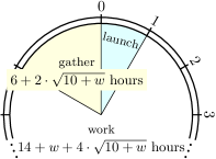
Figure 1: Schematic representation of the clock states.

We divide the hours into three consecutive intervals (see Section 3): the launching interval $\mathchar 73\relax_{\text{launch}}$ (first hour), the working interval $\mathchar 73\relax_{\text{work}}$ ($14+w+4\cdot\sqrt{10+w}$ hours) and the gathering interval $\mathchar 73\relax_{\text{gather}}$ (last $6+2\cdot\sqrt{10+w}$ hours). We say that agent $u$ is in one of the intervals whenever its clock counter $\mathsf{clock}[u]$ is in that interval. If the agents are either all in $\mathchar 73\relax_{\text{gather}}$, all in $\mathchar 73\relax_{\text{work}}$, or all in $\mathchar 73\relax_{\text{launch}}$, we say the configuration is homogeneous. Finally, for two agents $u$ and $v$ we define a distance $d(u,v)=\min\{|\mathsf{clock}[u]-\mathsf{clock}[v]|,|Q|-|\mathsf{clock}[u]-\mathsf{clock}[v]|\}$ that takes the cyclic nature of the clock into account. This allows us to formally define synchronous configurations as follows.

Definition (Synchronous Configuration).

A configuration $C$ is called synchronous if and only if for all pairs of agents $(u,v)$ we have $d(u,v)<(7+2\cdot\sqrt{10+w})\cdot\tau$. Our clock works as follows. Assume agents $(u,v)$ interact. With two exceptions, agent $u$ increments its counter $\mathsf{clock}[u]$ by one minute modulo $|Q|$ (Equations 1 and 2). If, however, $u$ is in $\mathchar 73\relax_{\text{gather}}$ and $v$ is in $\mathchar 73\relax_{\text{launch}}$ then agent $u$ adopts $\mathsf{clock}[v]$ (Equation 3): we say the agent hops. If $u$ is in $\mathchar 73\relax_{\text{gather}}$ and $v$ is in $\mathchar 73\relax_{\text{work}}$ then agent $u$ returns to the beginning of the $\mathchar 73\relax_{\text{gather}}$ interval (Equation 4): we say that the agent resets itself. We define that agent $u$ receives a signal whenever its clock crosses the wrap-around from $\mathchar 73\relax_{\text{gather}}$ to $\mathchar 73\relax_{\text{launch}}$. Formally, our clock uses the following state transitions. $\displaystyle(q_{1},q_{2})\in(Q\setminus\mathchar 73\relax_{\text{gather}})\times Q\colon$ $\displaystyle(q_{1},q_{2})\rightarrow(q_{1}+1,q_{2})$ (step forward) (1) $\displaystyle(q_{1},q_{2})\in\mathchar 73\relax_{\text{gather}}\times\mathchar 73\relax_{\text{gather}}\colon$ $\displaystyle(q_{1},q_{2})\rightarrow(q_{1}+1\bmod|Q|,q_{2})$ (step forward) (2) $\displaystyle(q_{1},q_{2})\in\mathchar 73\relax_{\text{gather}}\times\mathchar 73\relax_{\text{launch}}\colon$ $\displaystyle(q_{1},q_{2})\rightarrow(q_{2},q_{2})$ (hopping) (3) $\displaystyle(q_{1},q_{2})\in\mathchar 73\relax_{\text{gather}}\times\mathchar 73\relax_{\text{work}}\colon$ $\displaystyle(q_{1},q_{2})\rightarrow(|\mathchar 73\relax_{\text{launch}}|+|\mathchar 73\relax_{\text{work}}|,q_{2})$ (reset) (4)

On an intuitive level, the clock works as follows. Assume the clock is synchronized and all agents are in $\mathchar 73\relax_{\text{launch}}$. Now consider the next $k=\operatorname{\Theta}\bigl{(}n\cdot|Q|\bigr{)}$ interactions. All agents step forward according to Equation 1 until they reach $\mathchar 73\relax_{\text{gather}}$. The maximum distance between any agents grows during the $k$ interactions but it is still bounded by $\operatorname{\operatorname{\mathchar 79\relax}}\bigl{(}\sqrt{k/n}\bigr{)}=\operatorname{\operatorname{\mathchar 79\relax}}\bigl{(}\sqrt{|w|\cdot\log n}\bigr{)}$, w.h.p. Hence, due to the choice of $w$ there is no agent left behind in $\mathchar 73\relax_{\text{launch}}$ when the first agent reaches $\mathchar 73\relax_{\text{gather}}$. Additionally, due to the size of $\mathchar 73\relax_{\text{gather}}$ when the last agent enters $\mathchar 73\relax_{\text{gather}}$ all of the other agents are still in $|\mathchar 73\relax_{\text{gather}}|$. As soon as the first agent reaches $\mathchar 73\relax_{\text{launch}}$, Equation 3 (agents hop onto agents in $\mathchar 73\relax_{\text{launch}}$) ensures that all agents start the next phase without a large gap. Hence, there is an interaction after which all agents are in $|\mathchar 73\relax_{\text{launch}}|$ which brings us back to our initial configuration (all agents in $\mathchar 73\relax_{\text{launch}}$).

Now we consider an asynchronous configuration $C_{t}$ where the agents can be arbitrarily distributed over the $|Q|$ states of the clock. The main idea for the recovery of our clock is as follows. We show that after $\operatorname{\mathchar 79\relax}(n\log n)$ interactions there is a time $t$ where $\mathchar 73\relax_{\text{launch}}$ is empty. After $\operatorname{\mathchar 79\relax}(n\log n)$ additional steps most of the agents are in $\mathchar 73\relax_{\text{gather}}$: agents cannot hop since $\mathchar 73\relax_{\text{launch}}$ is empty, and they reset as soon as they interact with an agent in $\mathchar 73\relax_{\text{work}}$. They enter $\mathchar 73\relax_{\text{launch}}$ as soon as the first agent crosses $0$ by increasing its clock counter.

We will show that the following two properties hold for our clock.

Theorem 1.

Let $t_{1},t_{2}$ with $t_{1}\leq t_{2}$ be two points in time and assume that the configuration $C_{t_{1}}$ at time $t_{1}$ is a homogeneous launching configuration and $t_{2}-t_{1}\leq n^{c}$. Then the clock counters of the agents implement a synchronous $(\tau,w)$-phase clock in the time interval $[t_{1},t_{2}]$ w.h.p.

Theorem 2.

The clock counters of the agents implement a $\mathopen{}\mathclose{{}\left(\operatorname{\operatorname{\mathchar 79\relax}}\bigl{(}n\cdot\log n\bigr{)},\operatorname{\Omega}\bigl{(}\text{poly }n\bigr{)}}\right)$-loosely-stabilizing $\mathopen{}\mathclose{{}\left(\operatorname{\Theta}\bigl{(}\log n\bigr{)},w}\right)$-phase clock.

We prove Theorem 1 in Section 4 and Theorem 2 in Section 5.

Auxiliary Results

The one-way-epidemic is a population protocol with state space $\set{0,1}$ and transitions $(q_{1},q_{2})\rightarrow(\max\mathopen{}\mathclose{{}\left(q_{1},q_{2}}\right),q_{2})$. An agent in state $0$ is called susceptible and an agent in state $1$ is called infected. We say agent $u$ infects agent $v$ if $u$ is infected and initiates an interaction with $v$. The following result is folklore, see, e.g., [7]. Additional details can be found in LABEL:apx:one-way-epidemic.

Lemma 1 (One-way-epidemic).

Assume an agent starts the one-way epidemic in step $1$. All agents are infected after $t=\tau/4\cdot n$ many steps with probability at least $1-n^{-(7+2c)}$.

The following lemma bounds the number of interactions initiated by some fixed agent $u$ among a sequence of $t$ interactions. It is used throughout Sections 4 and 5 and follows immediately from Chernoff bounds (see LABEL:thm:chernoff-bounds).

Lemma 2.

Consider an arbitrary sequence of $t$ interactions and let $X_{u}$ be the number of interactions initiated by agent $u$ within this sequence. Then

$$\Pr\mathopen{}\mathclose{{}\left[{X_{u}<(1+\delta)\cdot t/n}}\right]\geq 1-n^{-\frac{12\cdot(c+4)t\cdot\delta^{2}}{n\cdot\tau}}\quad\text{and}\quad\Pr\mathopen{}\mathclose{{}\left[{X_{u}>(1-\delta)\cdot t/n}}\right]\geq 1-n^{-\frac{18\cdot(c+4)t\cdot\delta^{2}}{n\cdot\tau}}.$$

4 Maintenance: Proof of Theorem 1

In this section we first show the following main result. At the end of the section we show how Theorem 1 follows from this proposition.

Proposition 1 (Maintenance).

Consider our $(\tau,w)$-phase clock for $n$ agents with $\tau=12\cdot(c+4)\cdot\ln n$ for any $c\geq 6$ and sufficiently large $w$. Let configuration $C_{t_{1}}$ be a homogeneous launching configuration. Then, with probability at least $1-n^{-(c+1)}$, there exists a $t_{2}=\operatorname{\Theta}\bigl{(}n\cdot w\cdot\log n\bigr{)}$ such that the following holds:

1. $C_{t_{1}+t_{2}}$ is a homogeneous launching configuration,

2. $\forall t\in[t_{1},t_{1}+t_{2}]$: $C_{t}$ is synchronous,

3. in the time interval $[t_{1},t_{1}+t_{2}]$ there exists a contiguous sequence of homogeneous working configurations of length $w\cdot\tau\cdot n$.

We split the proof of Proposition 1 into two parts, Lemmas 3 and 4. The formal proof follows.

Proof.

Assume the configuration $C_{t_{1}}$ at time $t_{1}$ is a homogeneous launching configuration. Statements 1 and 2 of Proposition 1 follow immediately from Lemmas 3 and 4:

• It follows from Lemma 3 that the agents transition via a sequence of synchronous configurations into a homogeneous gathering configuration within $\Theta(n\cdot w\cdot\log n)$ time w.h.p.

• It follow from Lemma 4 that the agents transition via a sequence of synchronous configurations back into a homogeneous launching configuration within $\Theta(n\cdot w\cdot\log n)$ further time w.h.p.

It remains to show Statement 3. Recall that in a synchronous configuration all pairs of agents have distance (w.r.t. the circular order modulo $|Q|$) at most $\Delta=(7+2\cdot\sqrt{10+w})\cdot\tau$. Since $|\mathchar 73\relax_{\text{work}}|=w\cdot\tau+2\Delta$ it immediately follows that there must be $w\cdot\tau\cdot n$ interactions where all agents are in $\mathchar 73\relax_{\text{work}}$. This concludes the proof. ∎

The following lemma establishes that w.h.p. all agents transition from a homogeneous launching configuration into a homogeneous gathering configuration via a sequence of synchronous configurations.

Lemma 3.

Let $C_{t}$ be a homogeneous launching configuration. Let $t^{\prime}=n\cdot\smash{\frac{|\mathchar 73\relax_{\text{launch}}|+|\mathchar 73\relax_{\text{work}}|}{1-\mathopen{}\mathclose{{}\left(2\cdot\sqrt{|\mathchar 73\relax_{\text{work}}|/\tau}}\right)^{-1}}}$. Then the following holds with probability at least $1-n^{-(c+1)}/2$:

1. $C_{t+t^{\prime}}$ is a homogeneous gathering configuration and

2. $\forall t^{\prime\prime}\in[t,t+t^{\prime}]:C_{t^{\prime\prime}}$ is synchronous.

Proof.

In the following we assume w.l.o.g.  $t=0$. We prove the two statements separately.

Statement 1

Our goal is to show that after $t^{\prime}$ interactions all agents are in $\mathchar 73\relax_{\text{gather}}$ when we start from a homogeneous launching configuration $C_{0}$ at time $t=0$. We first show that there is no agent left in $\mathchar 73\relax_{\text{launch}}$ when the first agent enters $\mathchar 73\relax_{\text{gather}}$. Let $t_{a}$ be the first interaction in which an agent enters $\mathchar 73\relax_{\text{gather}}$. Note that before $t_{a}$ all agents are either in $\mathchar 73\relax_{\text{launch}}$ or in $\mathchar 73\relax_{\text{work}}$ and thus the agents increase their counter by one whenever they initiate an interaction.

First we show that w.h.p. $t_{a}\geq 2\cdot\tau\cdot n$. Let $X_{u}(2\cdot\tau\cdot n)$ denote the number of interactions agent $u$ initiates before time $2\cdot\tau\cdot n$. From Lemma 2 it follows with $\delta=1$ that $X_{u}(2\cdot\tau\cdot n)<4\cdot\tau$ with probability at least $1-n^{-24\cdot(c+4)}$. Since $4\cdot\tau<|\mathchar 73\relax_{\text{work}}|$, it holds that $\mathsf{clock}[u](2\cdot\tau\cdot n)<|\mathchar 73\relax_{\text{launch}}|+|\mathchar 73\relax_{\text{work}}|$ in this case. Hence, agent $u$ has not yet reached $\mathchar 73\relax_{\text{gather}}$ with probability at least $1-n^{-24\cdot(c+4)}$ at time $t_{a}$. It follows from a union bound over all agents that no agent has reached $\mathchar 73\relax_{\text{gather}}$ with probability at least $1-n^{-24\cdot(c+4)+1}$ at time $t_{a}$.

Next we show that w.h.p. at time $2\cdot\tau\cdot n$ all agents have left $\mathchar 73\relax_{\text{launch}}$. As before, let $X_{u}(2\cdot\tau\cdot n)$ denote the number of interactions agent $u$ initiates before time $2\cdot\tau\cdot n$. From Lemma 2 it follows with $\delta=1$ that $X_{u}(2\cdot\tau\cdot n)>\tau$ with probability at least $1-n^{-36\cdot(c+4)}$. Since $\tau=|\mathchar 73\relax_{\text{launch}}|$, it holds that $\mathsf{clock}[u](t+2\cdot\tau\cdot n)\geq|\mathchar 73\relax_{\text{launch}}|$ in this case. Hence, agent $u$ has left $\mathchar 73\relax_{\text{launch}}$ with probability at least $1-n^{-36\cdot(c+4)}$ at time $t_{a}$. Again, it follows from a union bound over all agents that all agents have left $\mathchar 73\relax_{\text{launch}}$ with probability at least $1-n^{-36\cdot(c+4)+1}$ at time $t_{a}$.

Let now $t_{b}$ be the first interaction in which an agent enters the last minute of $\mathchar 73\relax_{\text{gather}}$ and observe that $t_{b}>t_{a}$. Then, w.h.p. no agent is in $\mathchar 73\relax_{\text{launch}}$ during the time interval $[t+t_{a},t+t_{b}]$. Therefore, agents cannot hop. Thus, by definition of $t_{b}$, no agent can leave $\mathchar 73\relax_{\text{gather}}$ before time $t_{b}$. Agents that initiate an interaction must therefore either increase their counter by one or reset.

First we show that w.h.p. $t_{b}>t^{\prime}$. From Lemma 2 it follows with $\delta=\mathopen{}\mathclose{{}\left(2\cdot\sqrt{|\mathchar 73\relax_{\text{work}}|/\tau}}\right)^{-1}$ that $X_{u}(t^{\prime})<|\mathchar 73\relax_{\text{work}}|+|\mathchar 73\relax_{\text{gather}}|$ with probability at least $1-n^{-3(c+4)}$. (Note that we use $(1+\delta)/(1-\delta)<1/(1-2\cdot\delta)$ for $\delta<0.5$ and $(|\mathchar 73\relax_{\text{launch}}+|\mathchar 73\relax_{\text{work}}|)/(1-2\cdot\delta)=|\mathchar 73\relax_{\text{work}}|+\frac{w+5\cdot\sqrt{10+w}+16}{\sqrt{10+w}+1}\cdot\tau<|\mathchar 73\relax_{\text{work}}|+|\mathchar 73\relax_{\text{gather}}|$.) Thus, $\mathsf{clock}[u](t^{\prime})\leq\mathsf{clock}[u](0)+X_{u}(t^{\prime})<|\mathchar 73\relax_{\text{launch}}|-1+|\mathchar 73\relax_{\text{work}}|+|\mathchar 73\relax_{\text{gather}}|$ (which is the last state of $\mathchar 73\relax_{\text{gather}}$) with probability at least $1-n^{-3(c+4)}$. By a union bound, this holds for all agents with probability at least $1-n^{-(3c+11)}$.

Next we show that w.h.p. at time $t_{b}$ all agents have reached $\mathchar 73\relax_{\text{gather}}$. From Lemma 2 it follows with $\delta=\mathopen{}\mathclose{{}\left(2\cdot\sqrt{|\mathchar 73\relax_{\text{work}}|/\tau}}\right)^{-1}$ that $X_{u}(t^{\prime})>|\mathchar 73\relax_{\text{launch}}|+|\mathchar 73\relax_{\text{work}}|$ with probability at least $1-n^{-9\cdot(c+4)/2}$. Thus, $\mathsf{clock}[u](t^{\prime})\geq\mathsf{clock}[u](0)+X_{u}(t^{\prime})>0+|\mathchar 73\relax_{\text{launch}}|+|\mathchar 73\relax_{\text{work}}|$, with probability at least $1-n^{-9\cdot(c+4)/2}$. By a union bound, this holds for all agents with probability at least $1-n^{-(17+9/2\cdot c)}$.

Together it follows that at time $t^{\prime}$ no agent has left $\mathchar 73\relax_{\text{gather}}$ but all agents have entered it with probability at least $1-n^{-(c+3)}$. Therefore, $C_{t^{\prime}}$ is a homogeneous gathering configuration.

Statement 2

Recall that a synchronous configuration $C$ is defined as a configuration where $\max_{(u,v)}\set{d(u,v)}<|\mathchar 73\relax_{\text{launch}}|+|\mathchar 73\relax_{\text{gather}}|$. As before, let $X_{u}(i)$ denote the number of interactions agent $u$ initiates before time $i$. Now fix a time $t\leq t^{\prime}$ and a pair of agents $(u,v)$ with $X_{u}(t)<X_{v}(t)$. We use Lemma 2 to bound the deviation of $X_{u}(t)$ and $X_{v}(t)$ at time $t$ as follows: $\Pr\mathopen{}\mathclose{{}\left[{X_{u}(t)>t/n-\mathopen{}\mathclose{{}\left|\mathchar 73\relax_{\text{gather}}}\right|/2}}\right]\geq 1-n^{-6(c+4)}$ and $\Pr\mathopen{}\mathclose{{}\left[{X_{v}(t)<t/n+\mathopen{}\mathclose{{}\left|\mathchar 73\relax_{\text{gather}}}\right|/2}}\right]\geq 1-n^{-4(c+4)}$. Therefore, $|X_{v}(t)-X_{u}(t)|<|\mathchar 73\relax_{\text{gather}}|$ with probability at least $1-n^{-4(c+4)}-n^{-6(c+4)}$.

Note that Lemma 2 allows us to bound the deviation in the numbers of interactions initiated by agents $u$ and $v$. However, this does not immediately give a bound on the difference of the clock counters $|\mathsf{clock}[v](t)-\mathsf{clock}[u](t)|$. To bound the deviation of clock counters (by $|\mathchar 73\relax_{\text{launch}}|+|\mathchar 73\relax_{\text{gather}}|$), we therefore distinguish three cases.

First, assume that neither $u$ nor $v$ have reached $\mathchar 73\relax_{\text{gather}}$ at time $t$. Then $\mathsf{clock}[u](t)=\mathsf{clock}[u](0)+X_{u}(t)$ and $\mathsf{clock}[v](t)=\mathsf{clock}[v](t)+X_{v}(t)$. Observe that by the assumption of the lemma, both $u$ and $v$ are in $\mathchar 73\relax_{\text{launch}}$ at time $t=0$ and thus $|\mathsf{clock}[v](0)-\mathsf{clock}[u](0)|<|\mathchar 73\relax_{\text{launch}}|$. Together with the above bound on $|X_{v}(t)-X_{u}(t)|$ we get $|\mathsf{clock}[v](t)-\mathsf{clock}[u](t)|<|\mathchar 73\relax_{\text{launch}}|+|\mathchar 73\relax_{\text{gather}}|$.

Secondly, assume that $u$ has not reached $\mathchar 73\relax_{\text{gather}}$ but $v$ has reached $\mathchar 73\relax_{\text{gather}}$ at time $t$. Then $\mathsf{clock}[u](t)=\mathsf{clock}[u](0)+X_{u}(t)$. For $\mathsf{clock}[v](t)$, however, it might have occurred that $v$ has reset in some interactions before time $t$. Nevertheless, the clock counter of $v$ is bounded by the number of initiated interactions such that $\mathsf{clock}[v](t)\leq\mathsf{clock}[v](t)+X_{v}(t)$. (Note that $v$ can only increment its $\mathsf{clock}[v]$ counter or reset its value; hopping is not possible since we have shown in the proof of the first statement that $\mathchar 73\relax_{\text{launch}}$ is empty when the first agent enters $\mathchar 73\relax_{\text{gather}}$.) Therefore, we get again $|\mathsf{clock}[v](t)-\mathsf{clock}[u](t)|<|\mathchar 73\relax_{\text{launch}}|+|\mathchar 73\relax_{\text{gather}}|$.

Finally, assume that both $u$ and $v$ are in $\mathchar 73\relax_{\text{gather}}$ at time $t$. Then $|\mathsf{clock}[v](t)-\mathsf{clock}[u](t)|\leq|\mathchar 73\relax_{\text{gather}}|<|\mathchar 73\relax_{\text{launch}}|+|\mathchar 73\relax_{\text{gather}}|$ is trivially true.

There are no further cases: in the proof of the first statement we have shown that all agents transition from a homogeneous launching configuration to a homogeneous gathering configuration during the time interval $[0,t^{\prime}]$. The result now follows from a union bound over all $o(n^{2})$ points in time $t\leq t^{\prime}$ and all $n\cdot(n-1)$ pairs of agents. ∎

The following lemma is the main technical contribution of this section. It establishes that w.h.p. all agents transition from a homogeneous gathering configuration into a homogeneous launching configuration via a sequence of synchronous configurations. Consider a homogeneous gathering configuration and recall that whenever an agent hops from $\mathchar 73\relax_{\text{gather}}$ into $\mathchar 73\relax_{\text{launch}}$ it adopts the state of the responder. The main difficulty is to show that all agents hop into $\mathchar 73\relax_{\text{launch}}$ before the first agent leaves $\mathchar 73\relax_{\text{launch}}$.

Lemma 4.

Let $C_{t}$ be a homogeneous gathering configuration. Then with probability at least $1-n^{-(c+1)}/2$ the following holds:

1. there exists a $t_{0}=\operatorname{\operatorname{\mathchar 79\relax}}\bigl{(}n\cdot\sqrt{w}\cdot\log n\bigr{)}$ such that the first agent enters $\mathchar 73\relax_{\text{launch}}$ at time $t+t_{0}$,

2. there exists a $t^{\prime}\leq\tau/4\cdot n$ such that $C_{t+t_{0}+t^{\prime}}$ is a homogeneous launching configuration,

3. $\forall t^{\prime\prime}\in[t,t+t^{\prime}]:C_{t^{\prime\prime}}$ is synchronous.

Proof.

First we prove that w.h.p. there exists a homogeneous launching configuration $C_{t^{\prime}}$.

Statement 1

Let $t_{0}$ be defined such that the first agent $u$ leaves $\mathchar 73\relax_{\text{gather}}$ at time $t+t_{0}$. Since $C_{t}$ is a homogeneous gathering configuration, $\mathchar 73\relax_{\text{launch}}$ is empty at time $t$ and hence agent $u$ can only leave $\mathchar 73\relax_{\text{gather}}$ by increasing its counter. In every interaction before time $t+t_{0}$ some agent has to increase its state by one. Thus $t_{0}\leq n\cdot|\mathchar 73\relax_{\text{gather}}|=\operatorname{\operatorname{\mathchar 79\relax}}\bigl{(}n\cdot\sqrt{w}\cdot\log n\bigr{)}$.

Statement 2

We continue our analysis at time $t_{0}$ and again assume w.l.o.g. for the sake of brevity of notation that $t_{0}=0$. Note that at that time exactly one agent is in state $0$ and all remaining agents are still in $\mathchar 73\relax_{\text{gather}}$. We show the following: there exists a time $\tilde{t}=\tau/4\cdot n$ such that at time $\tilde{t}$ all agents are in $\mathchar 73\relax_{\text{launch}}$ (Recall that $|\mathchar 73\relax_{\text{launch}}|=\tau\cdot n$).To do so we first define a simplified process with the same state space $Q$, however, we refer to the last state of $\mathchar 73\relax_{\text{launch}}$ as $\mathsf{stop}$. Agents in $\mathsf{stop}$ never change their state (which renders the states of $\mathchar 73\relax_{\text{work}}$ unreachable). The formal definition of the simplified process is as follows.

$$(q_{1},q_{2})\in(\mathchar 73\relax_{\text{launch}}\setminus\set{\mathsf{stop}})\times Q\colon (q_{1},q_{2})\rightarrow(q_{1}+1,q_{2})$$ (step forward)

$$(q_{1},q_{2})\in\mathchar 73\relax_{\text{gather}}\times\mathchar 73\relax_{\text{gather}}\colon (q_{1},q_{2})\rightarrow(q_{1}+1,q_{2})\bmod|Q|$$ (step forward)

$$(q_{1},q_{2})\in\mathchar 73\relax_{\text{gather}}\times\mathchar 73\relax_{\text{launch}}\colon (q_{1},q_{2})\rightarrow(q_{2},q_{2})$$ (hopping)

$$(q_{1},q_{2})\in\set{\mathsf{stop}}\times Q\colon (q_{1},q_{2})\rightarrow(q_{1},q_{2})$$ (stopping)

For this simplified process we show a lower bound: after $\tilde{t}=\operatorname{\Theta}\bigl{(}n\cdot\log n\bigr{)}$ interactions all agents are in $\mathchar 73\relax_{\text{launch}}$. Then we show (for the simplified process) an upper bound: in $C_{\tilde{t}}$ none of the agents are in state $\mathsf{stop}$. A simple coupling of the simplified process and the original process shows that under these circumstances none of the agents entered $\mathchar 73\relax_{\text{work}}$ for our original process. This finishes the proof with $t^{\prime}=\tilde{t}$.

Lower Bound. In the simplified process agents can enter $\mathchar 73\relax_{\text{launch}}$ either via hopping or by making enough steps forward on their own. From Lemma 1 it follows that all agents enter $\mathchar 73\relax_{\text{launch}}$ after at most $\tilde{t}=\tau/4\cdot n$ interactions with probability at least $1-n^{-(5+c)}$. (For the upper bound, one can simply discard setting the clock counter to zero when an agent enters $\mathchar 73\relax_{\text{launch}}$ by increasing its counter.) Showing that none of the agents are in state $\mathsf{stop}$ is much harder. Due to the hopping the clock counters of agents in $\mathchar 73\relax_{\text{launch}}$ are highly correlated. Nevertheless, we can show that the clock counters of each agent can be majorized by independent binomially distributed random variables as follows.

Upper Bound. Let $u_{i}$ be the $i$’th agent that enters $\mathchar 73\relax_{\text{launch}}$ and let $t_{i}$ be the time when $u_{i}$ enters $\mathchar 73\relax_{\text{launch}}$. Let furthermore $X_{i}(t)$ be a random variable for the clock counter of agent $u_{i}$ in $\mathchar 73\relax_{\text{launch}}$ in the time interval $[0,t]$. Formally, we define for a time step $t$ that $X_{i}(t)=0$ if $u_{i}$ is in $\mathchar 73\relax_{\text{gather}}$ and $X_{i}(t)=\mathsf{clock}[u_{i}](t)$ if $u_{i}$ is in $\mathchar 73\relax_{\text{launch}}$. We show by induction on $i$ that $X_{i}(t)$ is majorized by a random variable $Z_{i}(t)$ with binomial distribution $Z_{i}(t)\sim\operatorname{Bin}\mathopen{}\mathclose{{}\left(t,1/n\cdot(1+1/(n-1))^{i-1}}\right)$. Ultimately, our goal is to apply Chernoff bounds to $Z_{i}(\tilde{t})$ which shows that agent $u_{i}$ does not reach $\mathsf{stop}$ w.h.p. The statement for the simplified process then follows from a union bound over all agents w.h.p.

Base Case. For the base case we consider all agents that enter $\mathchar 73\relax_{\text{launch}}$ on their own by incrementing their counters to $0$ (modulo $|Q|$) in $\mathchar 73\relax_{\text{gather}}$. Fix such an agent $u_{i}$. It holds that $X_{i}(t)$ for $t\geq t_{i}$ has binomial distribution $X_{i}(t)\sim\operatorname{Bin}(t-t_{i},1/n)$. Therefore, $X_{i}(t)\prec Z_{i}(t)$ as claimed. (Intuitively, this means that the clock counter of any other agent $u_{i}$ with $i>1$ that enters $\mathchar 73\relax_{\text{launch}}$ at time $t_{i}>0$ is majorized by the clock counter of an agent which enters $\mathchar 73\relax_{\text{launch}}$ at time $t_{1}=0$ and increments its counter with probability $1/n$.)

Induction Step. For the induction step we now consider all agents that enter $\mathchar 73\relax_{\text{launch}}$ by hopping onto some other agent in $\mathchar 73\relax_{\text{launch}}$. Fix such an agent $u_{i}$. Let $S_{i}$ be the event that agent $u_{i}$ is the $i$’th agent that enters $\mathchar 73\relax_{\text{launch}}$. Let furthermore $t_{i}$ be the time when $u_{i}$ enters $\mathchar 73\relax_{\text{launch}}$. We condition on $S_{i}$ and observe that agent $u_{i}$ enters $\mathchar 73\relax_{\text{launch}}$ by hopping onto some other agent $u_{j}\in\set{u_{1},\dots,u_{i-1}}$. Intuitively, we would now like to exploit the fact that the counter of agent $u_{i}$ is copied at time $t_{i}$ from agent $u_{j}$ such that $X_{i}(t_{i})=X_{j}(t_{i})$. Unfortunately, we must be extremely careful here: conditioning on $S_{i}$ alters the probability space! (For example, under $S_{i}$ the agent $u_{i}$ with $i\geq 3$ cannot initiate an interaction with agent $u_{1}$ before agent $u_{2}$ does, since $S_{i}$ rules out that $u_{i}$ enters $\mathchar 73\relax_{\text{launch}}$ before agent $u_{2}$.) We account for the modified probability space as follows.

Let $\Omega_{S_{i}}(t)$ be the probability space of possible interactions conditioned on $S_{i}$ at time $t\leq\tilde{t}$. Without the conditioning on $S_{i}$, the probability space $\Omega(t)$ at time $t$ contains all (ordered) pairs of agents with $|\Omega(t)|=n\cdot(n-1)$. When conditioning on $S_{i}$, the event $S_{i}$ rules out that agent $u_{i}$ interacts with any other agent $u_{j}\in\mathchar 73\relax_{\text{launch}}$ before time $t_{i}$. In particular, agent $u_{i}$ cannot interact with another agent $u_{j}$ with $j<i$ during the time interval $[t_{j},t_{i}]$. In order to give a lower bound on $|\Omega_{S_{i}}(t)|$, we exclude all $(n-1)$ interactions $(u_{i},u_{j})$ for $j\in[n]$ from $\Omega(t)$. Hence $|\Omega_{S_{i}}(t)|\geq n\cdot(n-1)-(n-1)=(n-1)^{2}$ for any time $t\leq t_{i}$. (The probability space after time $t_{i}$ is not affected by conditioning on $S_{i}$, but the majorization holds nonetheless.) We now consider the event $E_{\hat{t}}$ for $\hat{t}\leq t_{i}$ that the interaction at time $\hat{t}$ increments $X_{j}(t)$ by $1$ (recall that $u_{j}$ is the agent onto which $u_{i}$ hopped). It then holds for the reduced probability space $\Omega_{S_{i}}$ that $\Pr\mathopen{}\mathclose{{}\left[{E_{\hat{t}}|S_{i}}}\right]\leq\Pr\mathopen{}\mathclose{{}\left[{E_{\hat{t}}}}\right]\cdot|\Omega(t)|/|\Omega_{S_{i}}(t)|$. (Note that $\Omega_{S_{i}}$ is still a uniform probability space.) We calculate

$$\frac{|\Omega(t)|}{|\Omega_{S_{i}}(t)|}=\frac{n\cdot(n-1)}{(n-1)^{2}}=1+\frac{1}{n-1}$$

and get $\Pr\mathopen{}\mathclose{{}\left[{E_{\hat{t}}|S_{i}}}\right]\leq\Pr\mathopen{}\mathclose{{}\left[{E_{\hat{t}}}}\right]\cdot(1+{1}/{(n-1)})$ for $\hat{t}\leq t_{i}$. Therefore, we use the induction hypothesis (that describes $X_{j}(t_{i})$) and get $X_{i}(t_{i})\prec Z_{i}(t_{i})$, where $Z_{i}(t_{i})\sim\operatorname{Bin}\mathopen{}\mathclose{{}\left(t_{i},1/n\cdot\mathopen{}\mathclose{{}\left(1+1/(n-1)}\right)^{i-1}}\right)$. Similarly, we define $E_{\hat{t}}$ for $\hat{t}\geq t_{i}$ to be the event that $u_{i}$ increments its counter in $\mathchar 73\relax_{\text{launch}}$. Observe that $\Pr\mathopen{}\mathclose{{}\left[{E_{\hat{t}}}}\right]\leq 1/n$ for $\hat{t}>t_{i}$. It follows that $X_{i}(t)\prec Z_{i}(t)$ with distribution $Z_{i}(t)\sim\operatorname{Bin}(\tilde{t},1/n\cdot(1+1/(n-1))^{i-1})$ for $t\leq\tilde{t}$ as claimed. This concludes the induction.

Conclusions. From the induction it follows that for each agent $u_{i}$ the clock counter $\mathsf{clock}[u_{i}](\tilde{t})$ at time $\tilde{t}$ is majorized by a random variable $Z(\tilde{t})$ with binomial distribution $Z(\tilde{t})\sim\operatorname{Bin}(\tilde{t},e/n)$. (Note that we used the inequality $(1+1/(n-1))^{(n-1)}<e$.) From LABEL:thm:chernoff-bounds it follows that $\Pr\mathopen{}\mathclose{{}\left[{Z(\tilde{t})\geq\tau-1}}\right]\leq n^{-(c+4)}$. Finally, the proof for the simplified process follows from a union bound over all agents.

It is now straightforward to couple the actual phase clock process with the simplified process. Assume that we start both processes at time $0$ when exactly one agent is in state $0$. In the simplified process no agent reaches state $\tau$ in $\tau/4\cdot n$ interactions with probability at least $1-n^{-(c+3)}$. In this case, however, the simplified process and the actual phase clock process do not deviate and, in particular, no agent reaches the beginning of $\mathchar 73\relax_{\text{work}}$ in $\tau/4\cdot n$ many interactions. Thus, the configuration $C_{t^{\prime}}$ is a homogeneous launching configuration with probability at least $1-n^{-(c+3)}$.

Statement 3

By definition, all configurations where all agents are in $\mathchar 73\relax_{\text{gather}}\cup\mathchar 73\relax_{\text{launch}}$ are synchronous. ∎

We are now ready to put everything together and prove our first theorem.

Proof of Theorem 1.

The proof of Theorem 1 follows readily from the main result of this section, Proposition 1.

Assume the configuration at time $t_{1}$ is a synchronous launching configuration. Then from Proposition 1 it follows w.h.p. that after $t_{2}=\Theta(n\cdot w\cdot\log n)$ interactions the configuration $C_{t_{2}}$ is again a homogeneous launching configuration, and all configurations in $[t_{1},t_{2}]$ are synchronous. From Statement 3 it follows that no agent receives a signal in a contiguous subinterval $[t_{1}^{\prime},t_{2}^{\prime}]\subset[t_{1},t_{2}]$ of length $t_{2}^{\prime}-t_{1}^{\prime}=w\cdot\tau\cdot n$. This shows that we have w.h.p. the required overlap according to the definition of synchronous $(\tau,w)$-phase clocks.

From Lemma 4 it follows w.h.p. that all agents transition from a homogeneous gathering configuration into a homogeneous launching configuration within $\tau/4\cdot n$ interactions. Recall that whenever an agent crosses zero, it receives a signal. Therefore, when all agents transition from a homogeneous gathering configuration into a homogeneous launching configuration via a sequence of synchronous configurations, all agents receive exactly one signal, and the time between two signals of two agents $(u,v)$ is w.h.p. at most $\tau/4\cdot n$. This shows that we have w.h.p. the required bursts according to the definition of synchronous $(\tau,w)$-phase clocks.

Together, the counters of our clock implement a synchronous $(\tau,w)$-phase clock in $[t_{1},t_{2}]$ with probability $n^{-c}$. It follows from an inductive argument that the clock counters implement a synchronous $(\tau,w)$-phase clock during the $n^{c}$ interactions that follow time $t_{1}$ w.h.p. ∎

5 Recovery: Proof of Theorem 2

In this section we first show the following main result. At the end of the section we show how Theorem 2 follows from this proposition.

Proposition 2 (Recovery).

Consider our $(\tau,w)$-phase clock with $n$ agents and sufficiently large $c$ and $w$. Let $C_{t_{1}}$ be an arbitrary configuration. Then with probability at least $1-1/n$, there exists a $t_{2}=\operatorname{\operatorname{\mathchar 79\relax}}\bigl{(}n\cdot w\cdot\log n\bigr{)}$ such that $C_{t_{1}+t_{2}}$ is a homogeneous launching configuration.

We say a configuration is an almost homogeneous gathering configuration if no agent is in $\mathchar 73\relax_{\text{launch}}$ and at least $0.9\cdot n$ many agents are in $\mathchar 73\relax_{\text{gather}}$. We start our analysis by showing that within $t=\operatorname{\operatorname{\mathchar 79\relax}}\bigl{(}n\cdot w\cdot\log n\bigr{)}$ interactions, we reach an almost homogeneous gathering configuration $C_{t_{1}+t}$.

Lemma 5 (name=,restate=lemmaRecoveryOne,label=lem:any->emptylaunch).

Let $C_{t}$ be an arbitrary configuration. Then with probability at least $1-1/(3n)$, there exists a $t^{\prime}=\operatorname{\operatorname{\mathchar 79\relax}}\bigl{(}n\cdot w\cdot\log n\bigr{)}$ such that $C_{t+t^{\prime}}$ is an almost homogeneous gathering configuration.

Proof Sketch.

The main idea of the proof is as follows. If there are not too many agents in $\mathchar 73\relax_{\text{gather}}$, the reset rule prevents agents from reaching the end of $\mathchar 73\relax_{\text{gather}}$. Agents may still enter $\mathchar 73\relax_{\text{launch}}$ by hopping, but if no agent enters state $0$, eventually there is no agent left in state $0$ to hop on. Then the same argument applies to state $1$, and so on. Eventually, there are no agents left in $\mathchar 73\relax_{\text{launch}}$ to hop onto. This means the agents are trapped in $\mathchar 73\relax_{\text{gather}}$ until a sufficiently large number of agents enters $\mathchar 73\relax_{\text{gather}}$ which renders resetting quite unlikely again. The resulting configuration is what we call an almost homogeneous gathering configuration. ∎

Next, we show that from an almost homogeneous gathering configuration we reach a homogeneous gathering configuration in $\operatorname{\operatorname{\mathchar 79\relax}}\bigl{(}n\cdot w\cdot\log n\bigr{)}$ interactions. From Lemma 4 in Section 4 it then follows that we reach a homogeneous launching configuration in an additional number of $\operatorname{\mathchar 79\relax}(n\cdot\log n)$ interactions.

Lemma 6 (name=,restate=lemmaRecoveryTwo,label=lem:recovery:gather->launch).

Let $C_{t}$ be an almost homogeneous gathering configuration. Then with probability at least $1-1/(3n)$, there exists a $t^{\prime}=\operatorname{\Theta}\bigl{(}n\cdot w\cdot\ln n\bigr{)}$ such that $C_{t+t^{\prime}}$ is a homogeneous gathering configuration.

Proof Sketch.

If $C_{t}$ is an almost homogeneous gathering configuration, then there are no agents in $\mathchar 73\relax_{\text{launch}}$ and at least $0.9\cdot n$ many agents in $\mathchar 73\relax_{\text{gather}}$. Thus, agents cannot hop until an agent enters $\mathchar 73\relax_{\text{launch}}$ on its own. Now there are two cases. If no agent enters $\mathchar 73\relax_{\text{launch}}$ on its own before the last agent enters $\mathchar 73\relax_{\text{gather}}$, we are done: this is by definition of a homogeneous gathering configuration. Otherwise, we will show that a large fraction of agents leave $\mathchar 73\relax_{\text{gather}}$ together. This large fraction behaves similar as in the proof of the maintenance. The remaining agents have a small head start but then they are again trapped in $\mathchar 73\relax_{\text{gather}}$ until the bulk of agents arrives. Once the bulk of agents enters $\mathchar 73\relax_{\text{gather}}$ we have reached a homogeneous gathering configuration and all agents start to run through the clock synchronously. ∎

We are now ready to put everything together and show our second main theorem.

Proof of Theorem 2.

The proof of Theorem 2 follows readily from the main result of this section, Proposition 2. Observe that $\tau=\Theta(\log n)$. According to Proposition 2, our clock recovers to a homogeneous launching configuration in $\operatorname{\mathchar 79\relax}(n\cdot\log n)$ interactions. By Theorem 1, this marks the beginning of a time interval in which the agents implement a synchronous $(\tau,w)$-phase clock. It follows immediately from Theorem 1 that this interval has length $n^{c}$. Together, this implies that our $(\tau,w)$-phase clock is a $(\operatorname{\mathchar 79\relax}(n\cdot logn),\Omega(\operatorname{poly}n))$-loosely-stabilizing $(\Theta(\log n),w)$-phase clock. ∎

6 Adaptive Majority Problem

In this section we consider the adaptive majority problem introduced in [3] under the name robust comparison and defined as follows. At any time, every agent has as input either an opinion ($A$ or $B$) or it has no input, in which case we say it is undecided ($U$). During the execution of the protocol, the inputs to agents can change. In the adaptive majority problem, the goal is that all agents output the opinion which is dominant among all inputs. In this setting we present a loosely-stabilizing protocol that solves the adaptive majority problem.

Recall that the performance of a loosely-stabilizing protocol is measured in terms of the convergence time and the holding time. Note that the loose-stabilization comes from an application of our phase clock (see Section 3). The phase clocks guarantee synchronized phases for polynomial time. During this time we say a configuration $C$ is correct w.r.t. the adaptive majority problem if the following conditions hold. Suppose there is a sufficiently large bias towards one opinion. Then every agent in a correct configuration outputs the majority opinion. Otherwise, if there is no sufficiently large bias, we consider any output of the agents as correct. In this setting, we show the following result: We show that a $(\operatorname{\operatorname{\mathchar 79\relax}}\bigl{(}\log n\bigr{)},\operatorname{poly}n)$-loosely-stabilizing algorithm exists that solves adaptive majority, using $\operatorname{\operatorname{\mathchar 79\relax}}\bigl{(}\log n\bigr{)}$ states per agent.

6.1 Our Protocol

Our protocol is based on the $(\tau,w)$-phase clock defined in Section 3 with $w=566$. In addition to the states required by the clock, every agent $v$ has three variables $\mathsf{input}[v]$, $\mathsf{opinion}[v]$, and output $\mathsf{output}[v]$. The variable $\mathsf{input}[v]$ always reflects the current input to the agent, $\mathsf{opinion}[v]$ holds the current opinion of agent $v$, and $\mathsf{output}[v]$ defines the current output value of agent $v$. All three variables take on values in $\set{A,B,U}$, where $A$ and $B$ stand for the corresponding opinions and $U$ stands for undecided.

We use the $(\tau,w)$-phase clock to synchronize the agents. Then it follows from Proposition 1 that all configurations are synchronous w.h.p. Observe that in a synchronous configuration for our choice of parameters the clock counters of agents do not deviate by more than $\Delta=55\cdot\tau$. This allows us to define three subphases of $\mathchar 73\relax_{\text{work}}$, where agents execute three different protocols, as follows. We split the working interval $\mathchar 73\relax_{\text{work}}$ into six contiguous subintervals of equal length. The clock counters $\mathsf{clock}[u]$ allows us to define a simple interface to the phase clock for each agent $u$ as follows. The variable $\mathsf{subphase}[u]$ for each agent $u$ is then defined as follows. We set $\mathsf{subphase}[u]=1$ if $\mathsf{clock}[u]$ is in the first subinterval of $\mathchar 73\relax_{\text{work}}$, $\mathsf{subphase}[u]=2$ if $\mathsf{clock}[u]$ is in the third subinterval of $\mathchar 73\relax_{\text{work}}$, and $\mathsf{subphase}[u]=3$ if $\mathsf{clock}[u]$ is in the fifth subinterval of $\mathchar 73\relax_{\text{work}}$. Otherwise, $\mathsf{subphase}[u]=\bot$. The clock now assures a clean separation into these subphases such that no two agents perform a different protocol at any time w.h.p. Additionally, we will show the overlap within each subphase is long enough such that the subprotocols for the corresponding subphases succeed w.h.p.

On an intuitive level, our protocol works as follows. At the beginning of the phase, the input is copied to the opinion variable. In the first protocol, the support of opinions $A$ and $B$ is amplified until no undecided agents are left. We call this the Pólya Subphase. In the second protocol, agents with opposite opinions cancel each other out, becoming undecided. We call this the Cancellation Subphase. Finally, in the third protocol the single remaining opinion is amplified again. We call this the Broadcasting Subphase. The resulting opinion is copied to the output variable after the working interval $\mathchar 73\relax_{\text{work}}$. Formally, our protocol is specified in Section 6.1.

1

2update $\mathsf{clock}[u]$ according to Equations 1, 2, 3 and 4 with $w=566$

3 if Agent $u$ receives a signal then

4      $\mathsf{opinion}[u]\leftarrow\mathsf{input}[u]$

5     

6      if $\mathsf{subphase}[u]=1\land\mathsf{opinion}[u]=U$ then

7           $\mathsf{opinion}[u]\leftarrow\mathsf{opinion}[v]$

8          

9           if $\mathsf{subphase}[u]=2\land\mathsf{opinion}[u]\neq\mathsf{opinion}[v]\land\mathsf{opinion}[u],\mathsf{opinion}[v]\neq U$ then

10                $\mathsf{opinion}[u],\mathsf{opinion}[v]\leftarrow U$

11               

12                if $\mathsf{subphase}[u]=3\land\mathsf{opinion}[u]=U$ then

13                     $\mathsf{opinion}[u]\leftarrow\mathsf{opinion}[v]$

14                    

15                     if $\mathsf{clock}[u]\geq|\mathchar 73\relax_{\text{launch}}|+|\mathchar 73\relax_{\text{work}}|$ then

16                          $\mathsf{output}[u]\leftarrow\mathsf{opinion}[u]$

17                         

18                         

Result and Notation

In the remainder of this section, we let $A_{t}$ and $B_{t}$ denote the number of agents $u$ with $\mathsf{opinion}[u]=A$ and $\mathsf{opinion}[u]=B$, respectively, at time $t$. Analogously, we let $A_{t}^{\text{{in}}}$ and $B_{t}^{\text{{in}}}$ denote the number of agents $u$ with $\mathsf{input}[u]=A$ and $\mathsf{input}[u]=B$, respectively, at time $t$. We now state our main result for this section, where we assume w.l.o.g. that $A$ is the majority and $B$ is the minority opinion.

Theorem 3.

21                         Section 6.1 is a $(\operatorname{\operatorname{\mathchar 79\relax}}\bigl{(}n\log n\bigr{)},\operatorname{\Omega}\mathopen{}\mathclose{{}\left(\operatorname{poly}{n}}\right))$-loosely stabilizing adaptive majority protocol.

6.2 Analysis

23                         In the following analysis, we consider an arbitrary but fixed phase. We condition on the event that the clock is synchronized according to Proposition 1 during that phase. We show the following main result, and later in this section we describe how Theorem 3 follows from it this proposition. The proofs for the statements in this section can be found in LABEL:apx:majority.

Proposition 3 (name=,restate=promajority,label=pro:adaptive-majority).

Assume that at time $t_{1}$ the clocks are in a homogeneous launching configuration and we have $A_{t_{1}}\geq\alpha\cdot\log n$ and $A_{t_{1}}\geq\mathopen{}\mathclose{{}\left(1+\beta}\right)\cdot B_{t_{1}}$. If $\alpha$ and $\beta$ are large enough constants, then there exists a $t_{2}=\Theta(n\cdot w\cdot\log n)$ such that all agents output $A$ in configuration $C_{t_{1}+t_{2}}$ with probability $1-n^{-c}$.

25                         The analysis is split into three parts, one for the Pólya Subphase, one for the Cancellation Subphase, and one for the Broadcasting Subphase. First, we assume that no changes in the input occur. This highlights the simplicity of the application of our phase clock. Then we generalize our results: we adopt the undecided state dynamics introduced in [8], and show how we can tolerate input changes at various rates.

26                         Observe that from the guarantees of the phase clock in Theorem 1 we get a strict separation between the subphases: no two agents can be more than $1/6$ of $\mathchar 73\relax_{\text{work}}$ apart. Furthermore we know that every agent has copied its input at the beginning of the phase before the first agent enters the first subphase. At last the total time for the three subphases (including the separation time) is sufficiently large such that every agent has finished its work before the next phase starts.

27                         When we refer to a distribution before a subphase, we mean the distribution at the time just before the first agent performs an interaction in that subphase. Analogously, when we refer to a distribution after a subphase, we mean the distribution at the time when the last agent has performed an interaction in that subphase. Recall that in the following analysis, we let $A_{t}$ and $B_{t}$ denote the number of agents $u$ with $\mathsf{opinion}[u]=A$ and $\mathsf{opinion}[u]=B$, respectively, at time $t$. Furthermore, we let $s_{i}$ and $e_{i}$ (for start and end) be the first and the last time, respectively, when an agent performs an interaction in the $i$’th subphase.

Subphases

We first consider the Pólya Subphase, where we model the process by means of so-called Pólya urns. Pólya urns are defined as follows. Initially, the urn contains $a$ red balls and $b$ blue balls. In each step, a ball is drawn uniformly at random from the urn. The ball’s color is observed, and it is returned into the urn along with an additional ball of the same color. The Pólya-Eggenberger distribution $\operatorname{PE}(a,b,m)$ describes the total number of red balls after $m$ steps of this urn process.

29                         This observation allows us to apply concentration bounds to the opinion distribution after the Pólya Subphase. Recall that $s_{1}$ and $e_{1}$ are the first and the last time steps, respectively, when an agent performs an interaction in the Pólya Subphase. We get the following lemma.

Lemma 7 (name=,restate=lempolya,label=lem:polya).

Let $a=A_{s_{1}-1}$ and $b=B_{s_{1}-1}$. For any constant $\beta>0$ there exists a constant $\alpha$ such that if $a>\alpha\cdot\log n$ and $a>(1+\beta)\cdot b$ then $A_{e_{1}}-B_{e_{1}}=\operatorname{\Omega}\mathopen{}\mathclose{{}\left(n}\right)$ with probability at least $1-n^{-(c+2)}$.

Next we consider the Cancellation Subphase. The goal is to remove any occurrence of the minority opinion. Whenever an agent with opinion $A$ interacts with another agent with opinion $B$, both agents become undecided. Formally, we show the following lemma.

Lemma 8 (name=,restate=lemcancellation,label=lem:cancellation).

If $A_{s_{2}-1}-B_{s_{2}-1}=\operatorname{\Omega}\mathopen{}\mathclose{{}\left(n}\right)$ then $A_{e_{2}}=\operatorname{\Omega}\mathopen{}\mathclose{{}\left(n}\right)$ and $B_{e_{2}}=0$ with probability at least $1-n^{-(c+2)}$.

Finally we consider the Broadcasting Subphase. The goal is to spread the (unique) remaining opinion to all other agents. Whenever an undecided agent $u$ interacts with another agent $v$ that has an opinion, agent $u$ adopts the opinion of agent $v$. This leads to a configuration where every agent has the majority opinion w.h.p. Formally, we show the following lemma.

Lemma 9 (name=,restate=lembroadcasting,label=lem:broadcasting).

If $A_{e_{2}}=\operatorname{\Omega}\mathopen{}\mathclose{{}\left(n}\right)$ and $B_{e_{2}}=0$, then $A_{e_{3}}=n$ and $B_{e_{3}}=0$ with probability at least $1-n^{-(c+2)}$.

33                         We have now everything we need to prove LABEL:pro:adaptive-majority.

Proof of LABEL:pro:adaptive-majority.

We assume the configuration at time $t_{1}$ is a homogeneous launching configuration. From Proposition 1 it follows that all configurations in the time interval $[t_{1},t_{1}+t_{2}]$ for some $t_{2}=\Theta(n\cdot w\cdot\log n)$ are synchronous with probability at least $1-n^{-(c+1)}$. This means that the three subphases are strictly separated as explained above. It therefore follows, each with probability at least $1-n^{-(c+2)}$,

• from LABEL:lem:polya that after the Pólya Subphase no agent is undecided,

• from LABEL:lem:cancellation that after the Cancellation Subphase no agent has opinion $B$, and

• from LABEL:lem:broadcasting that after the Broadcasting Subphase all agents have opinion $A$.

Once all agents have opinion $A$, this becomes the output when the agents enter $\mathchar 73\relax_{\text{gather}}$. Together, this shows that all agents output the majority opinion after $\Theta(n\cdot w\cdot\log{n})$ interactions with probability at least $1-n^{-c}$. ∎

34                         With LABEL:pro:adaptive-majority we can now prove Theorem 3 as follows.

Proof of Theorem 3.

We first show recovery. Note that we do not (yet) consider input changes. Fix a time $t_{1}$ and assume the agents are in an arbitrary configuration at time $t_{1}$. From Theorem 2 it follows the clocks enter a synchronous configuration within $\operatorname{\operatorname{\mathchar 79\relax}}(n\log n)$ interactions and stay in synchronous configurations for $\operatorname{poly}n$ time w.h.p.

36                         Fix a synchronized phase $i<\operatorname{poly}n$. It follows from LABEL:pro:adaptive-majority that all agents enter a correct configuration at the end of phase $i$ with probability at least $1-n^{-c}$. (Recall that in a correct configuration all agents have to output the majority opinion if there is a sufficiently large bias. Without a bias, any output constitutes a correct configuration.)

37                         From the guarantees of the phase clock it follows that the first synchronized phase starts within $\operatorname{\mathchar 79\relax}(n\log n)$ time after time $t_{1}$ w.h.p. This shows a convergence time of $\operatorname{\mathchar 79\relax}(n\log n)$. From a union bound over at most $n^{c-1}$ phases it follows that the protocol is in a correct configuration for $\operatorname{poly}n$ interactions w.h.p. This shows a holding time of $\operatorname{poly}n$. Together, this concludes the proof. ∎

Improving the Bound

In order to show-case the simplicity of the application of our phase clock, we have presented a simplistic protocol, where we assumed a constant factor bias towards the majority opinion. We now show how to obtain a tighter result: we replace the Cancellation Subphase and the Broadcasting Subphase (lines 6 to 9 in Section 6.1) with the undecided state dynamics introduced in [8].

The undecided state dynamics is defined as follows. Each agent is in one of three states, $x$, $y$, or $b$. If an agent $u$ with opinion $x$ ($y$, resp.) interacts with another agent $v$ with opinion $y$ ($x$, resp.), agent $u$ enters the blank state $b$. If an agent $u$ in state $b$ interacts with another agent $v$ in state $x$ or $y$, $u$ adopts $v$’s state. When adopted to our problem, the values $A$, $B$, $U$ of variable $\mathsf{opinion}[u]$ at agent $u$ translate directly to states $x$, $y$, and $b$, respectively. The undecided state dynamics converge to the correct majority w.h.p. even if the multiplicative bias is much smaller than a constant fraction. Formally, we show the following statement.

Observation 1 (name=,restate=proImprovedBounds,label=pro:improved-bounds).

If we use the undecided state dynamics, LABEL:pro:adaptive-majority also holds for $\alpha=\operatorname{\Omega}\mathopen{}\mathclose{{}\left(\beta^{-2}}\right)$ provided that $\beta=\operatorname{\Omega}\mathopen{}\mathclose{{}\left(n^{-1/4+\varepsilon}}\right)$. This means that we can solve the adaptive majority problem with a multiplicative bias of $1+\beta=1+1/\log n=1+\operatorname{o}\bigl{(}1\bigr{)}$ and asymptotically at least $\operatorname{\Omega}\mathopen{}\mathclose{{}\left(\log^{2}n}\right)$ many agents (assuming sufficiently large constants). Hence we match the results of [3].

Robustness Against Input Changes

41                         We finally investigate the effect of input changes, introduced in [3] as leak transitions. Input changes affect the $\mathsf{input}[u]$ variable of an agent $u$: they convert an agent $u$ with majority input $\mathsf{input}[u]=A$ to an agent $u$ with minority input $\mathsf{input}[u]=B$. (Recall that we assume w.l.o.g. that $A$ is the majority and $B$ is the minority opinion.) Our main observation is the following. Let $r$ be the rate of input changes such that in each interaction an input changes with probability $r$. Assume that $r$ bounded and a sufficiently large bias $\beta$ towards the majority opinion is present. Then we show the following result.

Proposition 4 (name=,restate=proInputChanges,label=pro:input-changes).

Assume that at time $t_{1}$ he clocks are in a homogeneous launching configuration and we have $A_{t_{1}}\geq\alpha\cdot\log n$ and $A_{t_{1}}\geq\mathopen{}\mathclose{{}\left(1+\beta}\right)\cdot B_{t_{1}}$. Assume that the inputs change at rate $r$. If

$$\alpha =\operatorname{\Omega}\mathopen{}\mathclose{{}\left(\beta^{-2}}\right)\text{, }\quad\beta=\operatorname{\Omega}\mathopen{}\mathclose{{}\left(n^{-1/4+\varepsilon}}\right)\text{, \quad and }\quad r\leq\frac{\beta\cdot\alpha}{n}$$

then there exists a $t_{2}=\Theta(n\cdot w\cdot\log n)$ such that all agents output $A$ in configuration $C_{t_{1}+t_{2}}$ with probability $1-n^{-c}$.

43                         

44                         

Proof Sketch.

The main idea in the proof of LABEL:pro:input-changes is that we bound the number of input changes in $[t_{1},t_{2}]$ by a simple application of Chernoff bounds. Intuitively, if this number of input changes is at most a constant factor of the bias, we are done. Hence the result follows from the observation that the input configuration does not change quickly enough to turn over the bias: the output of the agents at the end of the phase, even though its calculation is based on an old configuration from the beginning of the phase, is still correct. The formal statement then follows from the previous analysis without input changes. ∎

45                         Finally, observe that also under presence of input changes we match the results of [3] for $r=1/n$, a multiplicative bias of $1+\beta=1+1/\log n$ and $\operatorname{\Omega}\mathopen{}\mathclose{{}\left(\log^{2}n}\right)$ many agents ($\alpha\geq\log n$).

46                         

Dan Alistarh, Bartlomiej Dudek, Adrian Kosowski, David Soloveichik, and Przemyslaw Uznanski. Robust detection in leak-prone population protocols. In DNA Computing and Molecular Programming - 23rd International Conference, DNA, volume 10467 of Lecture Notes in Computer Science, pages 155–171. Springer, 2017. doi:10.1007/978-3-319-66799-7\_11.

Dan Alistarh, Martin Töpfer, and Przemyslaw Uznanski. Comparison dynamics in population protocols. In Avery Miller, Keren Censor-Hillel, and Janne H. Korhonen, editors, PODC ’21: ACM Symposium on Principles of Distributed Computing, Virtual Event, Italy, July 26-30, 2021, pages 55–65. ACM, 2021. doi:10.1145/3465084.3467915.

Talley Amir, James Aspnes, and John Lazarsfeld. Approximate majority with catalytic inputs. In Quentin Bramas, Rotem Oshman, and Paolo Romano, editors, 24th International Conference on Principles of Distributed Systems, OPODIS 2020, December 14-16, 2020, Strasbourg, France (Virtual Conference), volume 184 of LIPIcs, pages 19:1–19:16. Schloss Dagstuhl - Leibniz-Zentrum für Informatik, 2020. doi:10.4230/LIPIcs.OPODIS.2020.19.

Dana Angluin, James Aspnes, Zoë Diamadi, Michael J. Fischer, and René Peralta. Computation in networks of passively mobile finite-state sensors. Distributed Comput., 18(4):235–253, 2006. doi:10.1007/s00446-005-0138-3.

Dana Angluin, James Aspnes, and David Eisenstat. Stably computable predicates are semilinear. In Proceedings of the Twenty-Fifth Annual ACM Symposium on Principles of Distributed Computing, PODC, pages 292–299. ACM, 2006. doi:10.1145/1146381.1146425.

Dana Angluin, James Aspnes, and David Eisenstat. Fast computation by population protocols with a leader. Distributed Comput., 21(3):183–199, 2008. doi:10.1007/s00446-008-0067-z.

Dana Angluin, James Aspnes, and David Eisenstat. A simple population protocol for fast robust approximate majority. Distributed Comput., 21(2):87–102, 2008. doi:10.1007/s00446-008-0059-z.

Dana Angluin, James Aspnes, David Eisenstat, and Eric Ruppert. The computational power of population protocols. Distributed Comput., 20(4):279–304, 2007. doi:10.1007/s00446-007-0040-2.

James Aspnes. Clocked population protocols. J. Comput. Syst. Sci., 121:34–48, 2021. doi:10.1016/j.jcss.2021.05.001.

Gregor Bankhamer, Petra Berenbrink, Felix Biermeier, Robert Elsässer, Hamed Hosseinpour, Dominik Kaaser, and Peter Kling. Fast consensus via the unconstrained undecided state dynamics, 2022. SODA 2022, to appear. arXiv:2103.10366.

Gregor Bankhamer, Robert Elsässer, Dominik Kaaser, and Matjaz Krnc. Positive aging admits fast asynchronous plurality consensus. In PODC ’20: ACM Symposium on Principles of Distributed Computing, pages 385–394. ACM, 2020. doi:10.1145/3382734.3406506.

Stav Ben-Nun, Tsvi Kopelowitz, Matan Kraus, and Ely Porat. An $o(\log^{3/2}n)$ parallel time population protocol for majority with $o(\log n)$ states. In Proceedings of the ACM Symposium on Principles of Distributed Computing, PODC 2020, Virtual Event, Italy, August 3-7, 2020, page to appear, 2020.

Petra Berenbrink, Robert Elsässer, Tom Friedetzky, Dominik Kaaser, Peter Kling, and Tomasz Radzik. Time-space trade-offs in population protocols for the majority problem. Distributed Computing, 2020. doi:10.1007/s00446-020-00385-0.

Petra Berenbrink, Robert Elsässer, Tom Friedetzky, Dominik Kaaser, Peter Kling, and Tomasz Radzik. Time-space trade-offs in population protocols for the majority problem. Distributed Comput., 34(2):91–111, 2021. doi:10.1007/s00446-020-00385-0.

Petra Berenbrink, George Giakkoupis, and Peter Kling. Optimal time and space leader election in population protocols. In Proccedings of the 52nd Annual ACM SIGACT Symposium on Theory of Computing, STOC, pages 119–129. ACM, 2020. doi:10.1145/3357713.3384312.

Janna Burman, Ho-Lin Chen, Hsueh-Ping Chen, David Doty, Thomas Nowak, Eric E. Severson, and Chuan Xu. Time-optimal self-stabilizing leader election in population protocols. In Avery Miller, Keren Censor-Hillel, and Janne H. Korhonen, editors, PODC ’21: ACM Symposium on Principles of Distributed Computing, Virtual Event, Italy, July 26-30, 2021, pages 33–44. ACM, 2021. doi:10.1145/3465084.3467898.

Anne Condon, Monir Hajiaghayi, David G. Kirkpatrick, and Ján Manuch. Approximate majority analyses using tri-molecular chemical reaction networks. Nat. Comput., 19(1):249–270, 2020. doi:10.1007/s11047-019-09756-4.

Shlomi Dolev and Jennifer L. Welch. Self-stabilizing clock synchronization in the presence of byzantine faults. J. ACM, 51(5):780–799, September 2004. doi:10.1145/1017460.1017463.

David Doty, Mahsa Eftekhari, Leszek Gąsieniec, Eric Severson, Grzegorz Stachowiak, and Przemysław Uznański. A time and space optimal stable population protocol solving exact majority, 2022. FOCS 2022, to appear. arXiv:2106.10201.

David Doty and David Soloveichik. Stable leader election in population protocols requires linear time. Distributed Computing, 31(4):257–271, 2018. doi:10.1007/s00446-016-0281-z.

Bartlomiej Dudek and Adrian Kosowski. Universal protocols for information dissemination using emergent signals. In Proceedings of the 50th Annual ACM SIGACT Symposium on Theory of Computing, STOC, pages 87–99. ACM, 2018. doi:10.1145/3188745.3188818.

Leszek Gasieniec and Grzegorz Stachowiak. Fast space optimal leader election in population protocols. In Proceedings of the Twenty-Ninth Annual ACM-SIAM Symposium on Discrete Algorithms, SODA, pages 2653–2667. SIAM, 2018. doi:10.1137/1.9781611975031.169.

Svante Janson. Tail bounds for sums of geometric and exponential variables. Statistics & Probability Letters, 135, 09 2017. doi:10.1016/j.spl.2017.11.017.

Norman Lloyd Johnson and Samuel Kotz. Urn Models and Their Application: An Approach to Modern Discrete Probability Theory. Wiley, 1977.

Algorithm 1 Interaction of agents $(u,v)$ in the adaptive majority protocol.

References

- 47[1] Dan Alistarh, James Aspnes, and Rati Gelashvili. Space-optimal majority in population protocols. In Proceedings of the Twenty-Ninth Annual ACM-SIAM Symposium on Discrete Algorithms, SODA, pages 2221–2239. SIAM, 2018. doi:10.1137/1.9781611975031.144.