Dimensional Interpolation for Random Walk

Abstract

We employ a simple and accurate dimensional interpolation formula for the shapes of random walks at $D=3$ and $D=2$ based on the analytically known solutions at both limits $D=\infty$ and $D=1$. The results obtained for the radii of gyration of an arbitrary shaped object are about $2\%$ error compared with accurate numerical results at $D=3$ and $D=2$. We also calculated the asphericity for a three-dimensional random walk using the dimensional interpolation formula. Result agrees very well with the numerically simulated result. The method is general and can be used to estimate other properties of random walks.

1 Introduction

The random walk problem is introduced by Pearson in 1905 ¹ and the following developed theory successfully implemented in different branches of science and engineering, for e.g., hydrodynamics ², astronomy ³, chemistry ⁴, polymer sciences ^{5, 6}, mathematics ⁷, biology ⁸, and economics ⁹. Many other topics in condensed matter physics include percolation clusters ¹⁰, lattice animals ^{11, 12}, disordered magnetic systems and spin glasses ¹³, anisotropy, and random fractals ¹⁴. The studies exploring the shapes of random walks have appeared, e.g. ^{15, 16}. Dimensional scaling offers simple solutions at $D=1$ and $D\to\infty$ limits, then often interpolates to obtain accurate results for $D=3$, in many areas of chemical physics ^{17, 18, 19, 20, 21, 22, 23, 24, 25, 26, 27}. Recently, we have used the dimensional interpolation formula developed by one of us ²⁸ to obtain the ground state energies for few electron atoms, simple diatomic molecules ²⁹ and also extended systems like metallic hydrogen ³⁰. Rudnick et al studied the random walks in high spacial dimensions ^{21, 31} and developed $1/D$ expansion to study the shape of a random walk in three dimensions. We employ a simple and accurate dimensional interpolation formula using dimensional limits $D=1$ and $D\to\infty$ to analyze the random walk problem at $D=3$ and $D=2$, and obtain physical quantities like radius of gyration and asphericity describing an arbitrary shaped two- and three-dimensional objects.

2 Basic dimensional interpolation formula

As a recapitulation, we start with the dimensional interpolation formula for atomic, molecular, and extended systems developed in our previous works. For dimensional scaling of atoms and molecules, the energy erupts to infinity as $D\to 1$ and vanishes as $D\to\infty$. Hence, we adopt scaled units (with hartree atomic units) whereby $E_{D}=\left(Z/\beta\right)^{2}\epsilon_{D}$ and $\beta=\frac{1}{2}\left(D-1\right)$, so the reduced energy $\epsilon_{D}$ remains finite in both limits.

The interpolation for atoms, developed in Ref. ²⁸, weights the dimensional limits by $\delta=1/D$, providing $\delta\epsilon_{1}$ and $\left(1-\delta\right)\epsilon_{\infty}$ in a simple analytic formula

$$\epsilon_{D}=\delta\epsilon_{1}+\left(1-\delta\right)\epsilon_{\infty}+\left[\epsilon_{D}^{(1)}-\delta\epsilon_{1}^{(1)}-\left(1-\delta\right)\epsilon_{\infty}^{(1)}\right]\lambda.$$ (1)

For a diatomic molecule, a different scaling scheme is used and illustrated. The rescaling of distances is:

$$R\to\delta R^{\prime}\text{ for }D\to 1;~{}R\to\left(1-\delta\right)R^{\prime}\text{ for }D\to\infty.$$ (2)

An approximation for $D=3$ (where $R=R^{\prime}$) emerges:

$$\epsilon_{3}\left(R^{\prime}\right)=\frac{1}{3}\epsilon_{1}\left(\frac{1}{3}R^{\prime}\right)+\frac{2}{3}\epsilon_{\infty}\left(\frac{2}{3}R^{\prime}\right),$$ (3)

interpolating linearly between the dimensional limits ^{32, 33, 34, 35}.

For the random walk problem an important quantity is the principal components of the radius of gyration $R_{i}^{2}$. These are one of the quantities for measuring the anisotropy of a $D$-dimensional random object. We propose to use the following interpolation formula for random walk problem

$$(R_{i}^{2})_{d}=\delta(R_{i}^{2})_{1}+\left(1-\delta\right)(R_{i}^{2})_{\infty},$$ (4)

where $\delta=1/D$, $D=$ dimension, and $(R_{i}^{2})_{D}$ is the $i$-th principle component of the radius of gyration.

3 Random walk at the large-D limit

There are a number of ways to measure the anisotropy of a random object generated by a three dimensional random walk. The shape of an arbitrary solid object in $D$-dimension is described by a quantity called the moment of inertia tensor, which is described as

$$T_{ij}=\frac{1}{N+1}\sum_{l=1}^{N+1}\left(x_{li}-\langle x_{i}\rangle\right)\left(x_{lj}-\langle x_{j}\rangle\right),$$ (5)

with

$$\langle x_{i}\rangle=\frac{1}{N+1}\sum_{l=1}^{N+1}x_{li},$$ (6)

where $x_{li}$ is the $i$-th coordinate of the particle after $l$ steps and $N$ is the total number of steps.

Eigenvalues of $\overset{\leftrightarrow}{T}$ are the square of the components of the radius of gyration $R_{i}^{2}$. The gyration tensor was first introduced by Solc and Stockmeyer in their study of random flight chain ³⁶. These principal components determine the size and shape of a solid object and also inertial properties ⁶. By convention $R_{1}^{2}\geq R_{2}^{2}\geq R_{3}^{2}...$ . The combination of principal radii of gyration is known as the square of the radius of gyration

$$R^{2}=R_{1}^{2}+R_{2}^{2}+R_{3}^{2}+...$$ (7)

The average value $\langle R^{2}\rangle$ for long, unrestricted open chain walks is calculated long ago, $R^{2}=N/6$ ³⁷ and for closed walks $R^{2}=N/12$ ^{38, 39}. From the principal radii of gyration we can compute asphericity or the asymmetry parameter of a solid object which is a one parameter measure to describe how much it is deformed from the perfect sphere ^{40, 41, 42}.

For a $N$-step random walk problem at $D=\infty$, Rudnick et al ²¹ showed that the moment of inertia tensor becomes:

$$(T_{\infty})_{ij} = \frac{i}{(N+1)^{2}}\left(N+1-j\right),\text{ for }i<j,\text{ and }1\leq i,j\leq(N+1),$$

$$= \frac{j}{(N+1)^{2}}\left(N+1-i\right),\text{ for }i>j,$$

$$= 0,\text{ otherwise. }$$

The eigenfunctions of $T_{ij}$ can be written as ³¹:

$$\psi_{n}(i)=\left(\frac{2}{N+1}\right)^{1/2}\sin\left(\frac{n\pi i}{N+1}\right),$$ (9)

and the corresponding eigenvalues are:

$$\lambda_{n}=(R_{n})^{2}=\frac{1}{4(N+1)}\left[\sin^{2}\left(\frac{n\pi}{2(N+1)}\right)\right]^{-1},$$ (10)

where $N$ is the total number of steps. For large $N$, the principal components of the radius of gyration becomes

$$\langle R_{n}^{2}\rangle=\lambda_{n}=\frac{N+1}{\pi^{2}n^{2}}\approx\frac{N}{\pi^{2}n^{2}}.$$ (11)

4 Random walk in one dimension

In one dimension, we have only two possible directions: forward and backward. For total number of steps = $N$, the probability of $m$ forward steps and $n$ backward steps can be written as

$$P(m,n)=\frac{1}{2^{N}}\frac{N!}{m!n!}.$$ (12)

For large $N$ the probability function can be defined as:

$$P(x)=\frac{2}{\sqrt{2\pi N}}e^{-\frac{x^{2}}{2N}},$$ (13)

where $x$ is the distance from the origin.

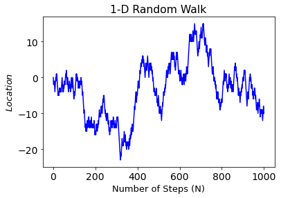
Figure 1: A random walk in one dimension with $1000$ steps. The x-axis describes the number of steps and the y-axis describes the position of the random walker after each step from the origin. The forward and backward directions are assumed to be positive and negative respectively.

We have developed a python program to simulate a random walk in one-dimension. For $N=1000$ steps an example of one dimensional random walk is plotted above in Fig.1.

We calculate the moment of inertia tensor $T$ from Eq.(5) which has one eigenvalue, $R_{1}^{2}$, the principle component of the radius of gyration. We repeat the simulation for $100,000$ times and take the average of all $R^{2}$’s and obtain $\langle R_{1}^{2}\rangle=166.2851794$.

The distribution of all $R_{1}^{2}$s obtained from different simulations is plotted below

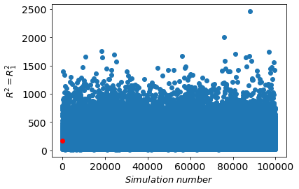
Figure 2: The distributio of all $R^{2}$s obtained from different simulations. The red point is the average $\langle R_{1}^{2}\rangle$ .

5 Random walk in two dimension

In two dimensions the particle can go in any of the two directions X and Y. We simulate a random walk in two spacial dimensions with $N=1000$ steps starting from the origin $(0,0)$. The simulation result of a two dimensional random walk is plotted below

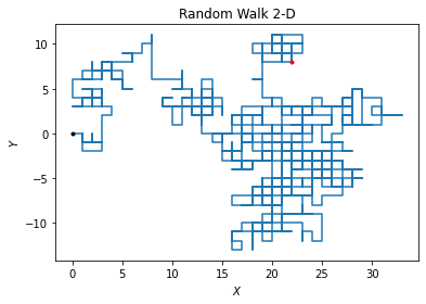
Figure 3: A random walk in two dimension with 1000 steps. The blue and red dots are beginning (origin) and ending points respectively.

We calculate the moment of inertia tensor $T_{ij}$ from Eq.(5), which has two eigenvalues, $R_{1}^{2},R_{2}^{2}$, the principle components of the radius of gyration. By convention $R_{1}^{2}\geq R_{2}^{2}$. We repeat the simulation for $100,000$ times. The distribution of all $R_{1}^{2},R_{2}^{2}$s obtained from different simulations is plotted below

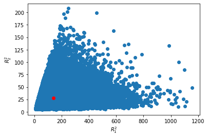
Figure 4: The distribution of all $R_{1}^{2},R_{2}^{2}$s obtained from different simulations. The red point is the average $\langle R^{2}\rangle$.

The averages of all $R_{i}^{2}$’s are given by $\langle R_{1}^{2}\rangle=138.94300$, $\langle R_{2}^{2}\rangle=27.90438$. The radius of gyration is given by: $R^{2}=(R_{1}^{2}+R_{2}^{2})=166.84739$.

Figure 5: plots of frequency and probability of $R_{1}^{2}$, as a function of its values occurring during different simulation.

6 Random walk in three dimension

In three dimensions the particle can go in any of the three X, Y, and Z directions.

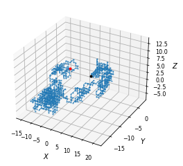
Figure 6: A random walk in three dimension with 1000 steps. The blue and red dots are beginning (origin) and ending points respectively.

We simulate a random walk in three spacial dimensions with $N=1000$ steps starting from the origin $(0,0,0)$. The simulation result of a three dimensional random walk is plotted above in Fig.6. We calculate the moment of inertia tensor $T_{ij}$ from Eq.(5), which has three eigenvalues, $R_{1}^{2},R_{2}^{2},R_{3}^{2}$, the principle components of the radius of gyration. By convention $R_{1}^{2}\geq R_{2}^{2}\geq R_{3}^{2}$. We repeat the simulation for $100,000$ times. The distribution of all $(R_{1}^{2},R_{2}^{2},R_{3}^{2})$s obtained from different simulations is plotted in Fig.7 and the frequency and probability distribution of the $R_{1}^{2}$ is plotted in Fig.8.

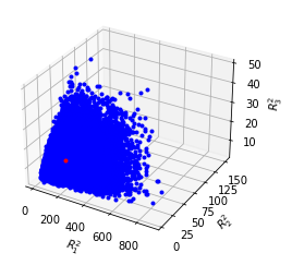
Figure 7: The distribution of all $(R_{1}^{2},R_{2}^{2},R_{3}^{2})$s obtained from different simulations. The red point is the average $\langle R^{2}\rangle$.

Figure 8: Frequency and probability distribution of $R_{1}^{2}$.

The averages of all $R_{i}^{2}$’s are given by $\langle R_{1}^{2}\rangle=126.82723$, $\langle R_{2}^{2}\rangle=28.68618$, $\langle R_{3}^{2}\rangle=10.57850$. The radius of gyration is given by: $R^{2}=(R_{1}^{2}+R_{2}^{2}+R_{3}^{2})=166.0919$.

7 Interpolation at $D=3$

We employ the interpolation formula in Eq.(4) developed by Herschbach ²⁸ for $R_{i}^{2}$ in three-dimension as follows:

$$(R_{i}^{2})_{3}=\frac{1}{3}(R_{i}^{2})_{1}+\frac{2}{3}(R_{i}^{2})_{\infty},$$ (14)

where $(R_{i}^{2})_{D}$ is the $i$-th component of the radius of gyration in D-dimension.

From Eq.(10) we see that

$$(R_{n})^{2}=\frac{1}{4(N+1)}\left[\sin^{2}\left(\frac{n\pi}{2(N+1)}\right)\right]^{-1},\text{ for }m=1,2,3,\text{ and }N=1000.$$ (15)

Therefore from Eq.(15) $(R_{1}^{2})_{\infty}=101.422588$. On the other hand $(R_{1}^{2})_{1}=166.2851794$.

From the above Eq. (14) we can calculate

$$(R_{1}^{2})_{3}=\frac{1}{3}(R_{1}^{2})_{1}+\frac{2}{3}(R_{1}^{2})_{\infty}={123.04345}.$$ (16)

The computer simulation of the three-dimensional random walk gives ${(R_{1}^{2})_{sim}=126.82723}$, which is a very close estimation with $2\%$ error.

In one dimension, there is only one component of the radius of gyration. Therefore, for interpolating the other component of the radius of gyration we have extrapolate the values of $R_{n}^{2}$ at one dimension for the calculation purpose. For $D=\infty$, and large $N$, the principal components of the radii are gyration are as follows:

$$R_{n}^{2}=\frac{1}{n^{2}}R_{1}^{2},$$ (17)

so that

$$(R_{1}^{2})_{\inf}:(R_{2}^{2})_{\inf}:(R_{3}^{2})_{\inf}=9:4:1.$$ (18)

On the other hand at $D=3$ in article ⁶ the authors showed that the following limiting ratios have been found to be approached for the large $N$ limit

$$\langle R_{1}^{2}\rangle:\langle R_{2}^{2}\rangle:\langle R_{3}^{2}\rangle=11.80:2.69:1$$ (19)

From the above Eq.s (18) and (19), we see that the ratios between the radius of gyration changes with the change of dimension. We propose a model for the dimensional dependence of $R_{n}^{2}$ as follows:

$$R_{n}^{2}=\left(\frac{1}{n^{2}(1+\frac{a_{n}}{D})}\right)R_{1}^{2},\text{ for }n=2,3,...,$$ (20)

where $a_{2},a_{3},...$ are constants and $D$ is the dimension. Now from the standard result at $D=3$ from Eq.(19) we can get two sets of equations, which has a solution $a_{2}=0.28996$ and $a_{3}=0.9333$.

With this ratios we can calculate the ratios between $R_{n}^{2}$ at $D=1$

$$(R_{2}^{2})_{1}=\frac{1}{5.15985}(R_{1}^{2})_{1},~{}\text{ and }~{}(R_{3}^{2})_{1}=\frac{1}{17.39997}(R_{1}^{2})_{1},$$ (21)

For $N=1000$, from Eq. (21), at $D=1$, we can calculate the following quantities $(R_{2}^{2})_{1}=32.2267$ and $(R_{3}^{2})_{1}=9.5566$. And from Eq. (15) at $D=\infty$, we compute the following quantities $(R_{2}^{2})_{\infty}=25.3557$ and $(R_{3}^{2})_{\infty}=11.26925$. With the values of $R_{i}^{2}$ at $D=1$ and $D=\infty$, we calculate $(R_{2}^{2})_{3}={27.64604}$ and the computer simulation gives $(R_{2}^{2})_{sim}={28.68618}$. Whereas, $(R_{3}^{2})_{3}={10.6983}$ and the computer simulation gives $(R_{3}^{2})_{sim}={10.5785}$.

The total radius of gyration from the interpolation is given by

$$(R^{2})_{3}=(R_{1}^{2})_{3}+(R_{2}^{2})_{3}+(R_{3}^{2})_{3}={161.38},$$ (22)

which is a fairly good estimation for the $(R^{2})_{sim}={166.0919}$, obtained from random walk simulation at $D=3$.

Now, we also calculate the ratios between the radii of gyrations obtained from the interpolation: $(R_{1}^{2})_{3}:(R_{2}^{2})_{3}:(R_{3}^{2})_{3}=11.5:2.58:1$, where as ratios between the radii of gyrations obtained from simulation is given by $(R_{1}^{2})_{sim}:(R_{2}^{2})_{sim}:(R_{3}^{2})_{sim}=11.98:2.71:1$.

The above estimates from dimensional interpolation are fairly close estimates, because none of the random number generators are perfect random number generator. Therefore the computer simulation of the random walk at $D=3$ is only an approximation for a perfect random walk in three dimensions. We expand our calculation by considering different step sizes to establish the validity of our interpolation formula. The averages are taken over $1000$ samples.

N= 10
Three dimensional simulation of all $R_{i}^{2}$’s are given by $\langle R_{1}^{2}\rangle=1.3640$, $\langle R_{2}^{2}\rangle=0.3242$, $\langle R_{3}^{2}\rangle=0.1139$. On the other hand from $D=\infty$ we have $(R_{1}^{2})_{\infty}=1.1221$ and from $D=1$ we have $(R_{1}^{2})_{1}=1.8226$. Using Eqs (15, 21) with the interpolation formula in Eq. (14) we can calculate $(R_{1}^{2})_{3}={1.35563}$, which is close to the value $\langle R_{1}^{2}\rangle={1.3640}$. Like the previous case we calculate the value of $R_{2}^{2}$ from dimensional interpolation which is equal to $(R_{2}^{2})_{3}=0.3086$, which agrees well with the computer simulation $(R_{2}^{2})_{sim}=0.3242$. For the third component $(R_{3}^{2})_{3}=0.1142$, which agrees well with the computer simulation $(R_{3}^{2})_{sim}=0.1140$.

N= 50
Three dimensional simulation of all $R_{i}^{2}$’s are given by $\langle R_{1}^{2}\rangle=6.3367$, $\langle R_{2}^{2}\rangle=1.4336$, $\langle R_{3}^{2}\rangle=0.54268$. On the other hand from $D=\infty$ we have $(R_{1}^{2})_{\infty}=5.1690$ and from $D=1$ we have $(R_{1}^{2})_{1}=8.29468$. Using Eqs (15, 21) with the interpolation formula in Eq. (14) we can calculate $(R_{1}^{2})_{3}={6.2109}$, which is close to the value $\langle R_{1}^{2}\rangle={6.3367}$. Like the previous case we calculate the value of $R_{2}^{2}$ from dimensional interpolation which is equal to $(R_{2}^{2})_{3}=1.3981676$, which agrees well with the computer simulation $(R_{2}^{2})_{sim}=1.4336$. For the third component $(R_{3}^{2})_{3}=0.5428$, which agrees well with the computer simulation $(R_{3}^{2})_{sim}=0.5427$.

N= 100
Three dimensional simulation of all $R_{i}^{2}$’s are given by $\langle R_{1}^{2}\rangle=12.7003$, $\langle R_{2}^{2}\rangle=2.9590$, $\langle R_{3}^{2}\rangle=1.0776$. On the other hand from $D=\infty$ we have $(R_{1}^{2})_{\infty}=10.2342$ and from $D=1$ we have $(R_{1}^{2})_{1}=17.5066$. Using Eqs (15, 21) with the interpolation formula in Eq. (14) we can calculate $(R_{1}^{2})_{3}={12.6584}$, which is close to the value $\langle R_{1}^{2}\rangle={12.7003}$. Like the previous case we calculate the value of $R_{2}^{2}$ from dimensional interpolation which is equal to $(R_{2}^{2})_{3}=2.83707$, which agrees well with the computer simulation $(R_{2}^{2})_{sim}=2.9590$. For the third component $(R_{3}^{2})_{3}=1.0939$, which agrees well with the computer simulation $(R_{3}^{2})_{sim}=1.0776$.

8 Interpolation at $D=2$

We employ the interpolation formula from Eq.(4) for $R_{i}^{2}$ in three-dimension as follows:

$$(R_{i}^{2})_{2}=\frac{1}{2}(R_{i}^{2})_{1}+\frac{1}{2}(R_{i}^{2})_{\infty},$$ (23)

where $(R_{i}^{2})_{D}$ is the $i$-th component of the radius of gyration in D-dimension.

Therefore from Eq.(10), $(R_{1}^{2})_{\infty}=101.422588$. On the other hand $(R_{1}^{2})_{1}=166.28518$.

From the above Eq. (23) we can calculate

$$(R_{1}^{2})_{2}=\frac{1}{2}(R_{1}^{2})_{1}+\frac{1}{2}(R_{1}^{2})_{\infty}={133.8539}.$$ (24)

From the computer simulation of the two-dimensional random walk gives ${(R_{1}^{2})_{sim}=138.94300}$, which is a fair estimation.

Using Eq. (21) we write the ratio between $R_{2}^{2}$ and $R_{1}^{2}$ at $D=1$

$$(R_{2}^{2})_{1}=\frac{1}{5.15985}(R_{1}^{2})_{1}.$$ (25)

For $N=1000$ from Eq. (25), at $D=1$, we calculate $(R_{2}^{2})_{1}=32.2267$. From Eq. (15) at $D=\infty$, we calculate the following quantities $(R_{2}^{2})_{\infty}=25.3557$. With the above data at $D=1$ and $D=\infty$, we compute $(R_{2}^{2})_{2}={28.7912}$ and the computer simulation gives $(R_{2}^{2})_{sim}={27.9044}$.

The total radius of gyration from the interpolation is given by

$$(R^{2})_{2}=(R_{1}^{2})_{2}+(R_{2}^{2})_{2}={162.6451},$$ (26)

which is a fairly good estimation for the $(R^{2})_{sim}={166.84739}$, obtained from random walk simulation in two dimensions.

Like the three dimensional case, we also calculate the ratios between the radii of gyrations obtained from the interpolation: $(R_{1}^{2})_{2}:(R_{2}^{2})_{3}=133.8539:28.7912=4.65:1$, whereas ratios between the radii of gyrations obtained from simulation is given by $(R_{1}^{2})_{sim}:(R_{2}^{2})_{sim}=138.9430:27.90438=4.97:1$. We expand our calculation by considering different step sizes to establish the validity of our interpolation formula at $D=2$. The averages are taken over $1000$ samples.

N= 50
Two dimensional simulation of all $R_{i}^{2}$’s are given by $\langle R_{1}^{2}\rangle=7.2121$, $\langle R_{2}^{2}\rangle=1.4513$. On the other hand from $D=\infty$ we have $(R_{1}^{2})_{\infty}=5.1690$ and from $D=1$ we have $(R_{1}^{2})_{1}=8.29468$. Using Eqs (15, 21) with the interpolation formula in Eq. (14) we can calculate $(R_{1}^{2})_{3}={6.7318}$, which is close to the value $\langle R_{1}^{2}\rangle={7.2121}$. Like the previous case we calculate the value of $R_{2}^{2}$ from dimensional interpolation which is equal to $(R_{2}^{2})_{2}=1.4505$, which agrees well with the computer simulation $(R_{2}^{2})_{sim}=1.4513$.

N= 100
Two dimensional simulation of all $R_{i}^{2}$’s are given by $\langle R_{1}^{2}\rangle=14.0010$, $\langle R_{2}^{2}\rangle=2.8198$. On the other hand from $D=\infty$ we have $(R_{1}^{2})_{\infty}=10.2342$ and from $D=1$ we have $(R_{1}^{2})_{1}=17.5066$. Using Eqs (15, 21) with the interpolation formula in Eq. (14) we can calculate $(R_{1}^{2})_{2}={13.8704}$, which is close to the value $\langle R_{1}^{2}\rangle={14.0010}$. Like the previous case we calculate the value of $R_{2}^{2}$ from dimensional interpolation which is equal to $(R_{2}^{2})_{2}=2.9760$, which agrees well with the computer simulation $(R_{2}^{2})_{sim}=2.8198$.

9 Asphericity

The radius of gyration is a measure of the average extent of a random walk. However, to get a better idea of its shape a quantity $A_{D}$ is defined, named the asphericity ^{40, 31, 42}. This quantity determines how much a solid object is deviated from the perfect sphere. For example for a perfect spherical object asphericity $A_{D}=0$, on the other hand this quantity has an upper bound of one, a limit that is reached when the walk is extended in one dimension only. Mathematically expression for $A_{D}$ is as follows:

$$A_{D}=\frac{\sum_{i>j}^{D}\left\langle\left(R_{i}^{2}-R_{j}^{2}\right)^{2}\right\rangle}{\left(D-1\right)\left\langle\left(\sum_{i=1}^{D}R_{i}^{2}\right)^{2}\right\rangle}$$ (27)

At the large $D$-dimension Rudnick et. al. ^{40, 31} showed that the expression of asphericity can be written as

$$A_{D}=\frac{2}{5}+\frac{12}{25D}+O\left(\frac{1}{D^{2}}\right).$$ (28)

For $D\to\infty$, $A_{\infty}=\frac{2}{5}$. On the other hand, for $D=1$, $A_{1}=1$.

In ^{43, 44} the authors introduces a dimensional interpolation formula with $D=0$ and $D=\infty$ and calculate the a quantity called asymmetry (similar to asphericity), which is defined as

$$\mathcal{A}_{D}=\frac{1}{D-1}\left\langle\frac{\sum_{i>j}^{D}\left(R_{i}^{2}-R_{j}^{2}\right)^{2}}{\left(\sum_{i=1}^{D}R_{i}^{2}\right)^{2}}\right\rangle.$$ (29)

Although both the above quantities measure the anisotropy, the asymmetry $\mathcal{A}_{D}$ is slightly different from the asphericity $A_{D}$, defined in Eq. (27). Because, the asphericity of each walk in the ensemble calculated first and then the result is averaged. Whereas, for calculating the asphericity $A_{D}$ we take the average over the numerator and denominator part separately. See ^{21, 41} for more details.

Eq. (28) gives a dimensional dependence of $A_{D}$ at the large-$D$ limit as a power series of $1/D$. Although this power series expression for $A_{D}$ does not produce the result at $D=1$, which is $A_{1}=1$. For the interpolation at $D=3$ we modify the above expression in Eq. (28) for $A_{D}$ for the large-$D$ limit, and use the result for $A_{D}$ at $D=1$ . We rewrite the expression for the asphericity in $D$-dimension:

$$A_{D}=\frac{2}{5}+\frac{a}{D}+\frac{a^{2}}{D^{2}}+\frac{a^{3}}{D^{3}}+...,$$ (30)

where $a$ is a parameter to be fixed from a known value of $A_{D}$ at a given dimension. For the calculation purpose we consider the terms up to the cubic order in $(a/D)$. For $D=1$, we know that $A_{D}=1$. We put this $D=1$ result in the above Eq. (30) and get the following condition for $a$

$$5a^{3}+5a^{2}+5a=3,$$ (31)

which has a solution $a=0.3894$. Now, putting back the value of $a$ and $D=3$ in Eq.(30) we obtain

$$A_{3}=0.5488.$$ (32)

We have performed numerical simulation of a random walk at $D=3$ with $N=1000$ steps. Then, we took an average over $100000$ samples and calculate the asphericity using Eq. (27) $A_{sim}=0.5240$, which is in close estimation with the above theoretical prediction.

10 Conclusion

The simplicity of the $D\to\infty$ limit attributed to the removal of the derivatives terms from the Hamiltonian in the case of electronic structure ³⁵. Thus one has to find the minimum energy of an effective potential. For the random walk, at $D\to\infty$ limit, the walker takes a step in along each $D$-dimensional axis. The simplicity of the $D=1$ limit keeps derivatives in a Hamiltonian and is a true hyperquantum limit. Combining these extreme partner limits delivers the dimensional interpolation formula. We have used the interpolation formula successfully for two-electron atoms ²⁸ and generalized it for few electron atoms, simple diatomic molecules ²⁹, and metallic hydrogen³⁰. In this article we implemented the dimensional interpolation formula for the random walks and calculated physical quantities like radii of gyration and asphericity in two and three dimensions to show its robustness in different topics in physics and chemistry.

The complexity of $N$-step random walk problem at $D=3$ is of order order $6^{N}$, where as in $D=1$, it is of the order $2^{N}$. Therefore, in $D=3$ the complexity of the simulation grows exponentially $(6^{N}/2^{N}=3^{N})$ with the number of steps and with the number of dimension. Whereas, for random walks at $D=\infty$ there is an analytical formula, which is described above. It is relatively easy to calculate the $D\to\infty$ and $D=1$ limits, so the interpolation formula can predict results for the physical dimensions, $D=2\text{ or }3$. The interpolation formula is general and might be used to obtain accurate results for other complex systems such as spin systems on different latices used extensively for magnetic materials and quantum computing simulations.

Authors’ information

ORCID IDs: Kumar Ghosh: 0000-0002-4628-6951, Sabre Kais: 0000-0003-0574-5346, Dudley Herschbach: 0000-0003-3225-0648. Note: The authors have no competing financial interest.

References

- Pearson 1905 Pearson, K. The problem of the random walk. Nature 1905, 72, 294
- Lebowitz and Montroll 1984 Lebowitz, J. L.; Montroll, E. W. Nonequilibrium phenomena. II-From stochastics to hydrodynamics. NASA STI/Recon Technical Report A 1984, 85, 43951
- Chandrasekhar 1943 Chandrasekhar, S. Stochastic problems in physics and astronomy. Reviews of modern physics 1943, 15, 1
- Domb and Joyce 1972 Domb, C.; Joyce, G. S. Cluster expansion for a polymer chain. Journal of Physics C: Solid State Physics 1972, 5, 956
- De Gennes and Gennes 1979 De Gennes, P. G.; Gennes, P. G. Scaling concepts in polymer physics; Cornell university press, 1979
- Šolc 1973 Šolc, K. Statistical mechanics of random-flight chains. IV. Size and shape parameters of cyclic, star-like, and comb-like chains. Macromolecules 1973, 6, 378–385
- Mandelbrot 1982 Mandelbrot, B. B. The fractal geometry of nature; W.H. Freeman New York, 1982; Vol. 1
- Codling et al. 2008 Codling, E. A.; Plank, M. J.; Benhamou, S. Random walk models in biology. Journal of the Royal society interface 2008, 5, 813–834
- Cooper 1982 Cooper, J. C. B. World stock markets: Some random walk tests. Applied Economics 1982, 14, 515–531
- Essam et al. 1972 Essam, J. W.; Domb, C.; Green, M. S. Phase transitions and critical phenomena. Phase Transit. Crit. Phenomena 1972, 2, 1583–1585
- Stauffer 1979 Stauffer, D. Scaling theory of percolation clusters. Physics reports 1979, 54, 1–74
- Aronovitz and Stephen 1987 Aronovitz, J.; Stephen, M. Universal features of the shapes of percolation clusters and lattice animals. Journal of Physics A: Mathematical and General 1987, 20, 2539
- Witten and Cates 1986 Witten, T. A.; Cates, M. E. Tenuous structures from disorderly growth processes. Science 1986, 232, 1607–1612
- Family et al. 1985 Family, F.; Vicsek, T.; Meakin, P. Are random fractal clusters isotropic? Physical review letters 1985, 55, 641
- Kuhn 1934 Kuhn, W. über die gestalt fadenförmiger moleküle in lösungen. Kolloid-Zeitschrift 1934, 68, 2–15
- Flory 1953 Flory, P. J. Principles of polymer chemistry; Cornell University Press, 1953
- Herschbach et al. 2012 Herschbach, D. R.; Avery, J. S.; Goscinski, O. Dimensional scaling in chemical physics; Springer Science & Business Media, 2012
- Goodson et al. 1992 Goodson, D. Z.; López-Cabrera, M.; Herschbach, D. R.; Morgan III, J. D. Large-order dimensional perturbation theory for two-electron atoms. J. Chem. Phys. 1992, 97, 8481–8496
- Zhen and Loeser 1993 Zhen, Z.; Loeser, J. Dimensional Scaling in Chemical Physics; Springer, 1993; pp 83–114
- Kais and Herschbach 1994 Kais, S.; Herschbach, D. R. The 1/Z expansion and renormalization of the large-dimension limit for many-electron atoms. J. Chem. Phys. 1994, 100, 4367–4376
- Rudnick and Gaspari 1987 Rudnick, J.; Gaspari, G. The shapes of random walks. Science 1987, 237, 384–389
- Loeser et al. 1991 Loeser, J. G.; Zhen, Z.; Kais, S.; Herschbach, D. R. Dimensional interpolation of hard sphere virial coefficients. J. Chem. Phys. 1991, 95, 4525–4544
- Kais and Herschbach 1993 Kais, S.; Herschbach, D. R. Dimensional scaling for quasistationary states. J. Chem. Phys. 1993, 98, 3990–3998
- Wei et al. 2008 Wei, Q.; Kais, S.; Herschbach, D. Dimensional scaling treatment of stability of simple diatomic molecules induced by superintense, high-frequency laser fields. J. Chem. Phys. 2008, 129, 214110
- Wei et al. 2007 Wei, Q.; Kais, S.; Herschbach, D. Dimensional scaling treatment of stability of atomic anions induced by superintense, high-frequency laser fields. J. Chem. Phys. 2007, 127, 094301
- Kais et al. 1994 Kais, S.; Sung, S. M.; Herschbach, D. R. Large-Z and-N dependence of atomic energies from renormalization of the large-dimension limit. Int. J. Quantum Chem. 1994, 49, 657–674
- Germann and Kais 1993 Germann, T. C.; Kais, S. Large order dimensional perturbation theory for complex energy eigenvalues. J. Chem. Phys. 1993, 99, 7739–7747
- Herschbach et al. 2017 Herschbach, D. R.; Loeser, J. G.; Virgo, W. L. Exploring Unorthodox Dimensions for Two-Electron Atoms. J. Phys. Chem. A 2017, 121, 6336–6340
- Ghosh et al. 2020 Ghosh, K. J. B.; Kais, S.; Herschbach, D. R. Unorthodox Dimensional Interpolations for He, Li, Be Atoms and Hydrogen Molecule. Frontiers in Physics 2020, 8, 331
- Ghosh et al. 2021 Ghosh, K. J. B.; Kais, S.; Herschbach, D. R. Dimensional interpolation for metallic hydrogen. Phys. Chem. Chem. Phys. 2021, 23, 7841–7848
- Rudnick et al. 1987 Rudnick, J.; Beldjenna, A.; Gaspari, G. The shapes of high-dimensional random walks. Journal of Physics A: Mathematical and General 1987, 20, 971
- Frantz and Herschbach 1988 Frantz, D. D.; Herschbach, D. R. Lewis electronic structures as the large-dimension limit for and molecules. Chemical physics 1988, 126, 59–71
- Tan and Loeser 1993 Tan, A. L.; Loeser, J. G. In Dimensional Scaling in Chemical Physics; Herschbach, D. R., Avery, J., Goscinski, O., Eds.; Springer Netherlands: Dordrecht, 1993; pp 230–255
- López-Cabrera et al. 1993 López-Cabrera, M.; Tan, A. L.; Loeser, J. G. Scaling and interpolation for dimensionally generalized electronic structure. J. Phys. Chem. 1993, 97, 2467–2478
- Loeser et al. 1994 Loeser, J. G.; Summerfield, J. H.; Tan, A. L.; Zheng, Z. Correlated electronic structure models suggested by the large-dimension limit. J. Chem. Phys 1994, 100, 5036–5053
- Šolc 1971 Šolc, K. Shape of a Random-Flight Chain. J. Chem. Phys 1971, 55, 335–344
- Debye 1946 Debye, P. The intrinsic viscosity of polymer solutions. J. Chem. Phys 1946, 14, 636–639
- Kramers 1946 Kramers, H. A. The behavior of macromolecules in inhomogeneous flow. J. Chem. Phys 1946, 14, 415–424
- Zimm and Stockmayer 1949 Zimm, B. H.; Stockmayer, W. H. The Dimensions of Chain Molecules Containing Branches and Rings. J. Chem. Phys 1949, 17, 1301–1314
- Theodorou and Suter 1985 Theodorou, D. N.; Suter, U. W. Shape of unperturbed linear polymers: polypropylene. Macromolecules 1985, 18, 1206–1214
- Rudnick and Gaspari 1986 Rudnick, J.; Gaspari, G. The aspherity of random walks. J. Phys. A: Math. Gen. 1986, 19, L191
- Aronovitz and Nelson 1986 Aronovitz, J. A.; Nelson, D. R. Universal features of polymer shapes. Journal de physique 1986, 47, 1445–1456
- Loeser and Herschbach 1996 Loeser, J. G.; Herschbach, D. In New Methods in Quantum Theory; Tsipis, C., Popov, V., Herschbach, D., Avery, J., Eds.; Kluwer Academic Pub: Dordrecht, 1996
- Herschbach 1996 Herschbach, D. R. Dimensional scaling and renormalization. International journal of quantum chemistry 1996, 57, 295–308