Continual Novelty Detection

Abstract

Novelty Detection methods identify samples that are not representative of a model’s training set thereby flagging misleading predictions and bringing a greater flexibility and transparency at deployment time. However, research in this area has only considered Novelty Detection in the offline setting. Recently, there has been a growing realization in the machine learning community that applications demand a more flexible framework - Continual Learning - where new batches of data representing new domains, new classes or new tasks become available at different points in time. In this setting, Novelty Detection becomes more important, interesting and challenging. This work identifies the crucial link between the two problems and investigates the Novelty Detection problem under the Continual Learning setting. We formulate the Continual Novelty Detection problem and present a benchmark, where we compare several Novelty Detection methods under different Continual Learning settings. We show that Continual Learning affects the behaviour of novelty detection algorithms, while novelty detection can pinpoint insights in the behaviour of a continual learner. We further propose baselines and discuss possible research directions. We believe that the coupling of the two problems is a promising direction to bring vision models into practice.

1 Introduction

Novelty or Out of Distribution or Anomaly Detection methods deal with the problem of detecting input data that are unfamiliar to a given model and out of its knowledge scope (Hendrycks & Gimpel, 2016) therefore avoiding misleading predictions and providing the model with a “no” option. In spite of the significant potential of the novelty detection problem in real-life scenarios, most novelty detection methods are designed and tested for detecting input data drawn from datasets that are very different from those used for training (e.g., training on CIFAR-10 and detecting SVHN images Lee et al. (2018)) in which the discrepancy between the datasets can be exploited rather than a difference in the represented objects. It has been noted that novel object detection is harder when they correspond to new categories from the same input domain (Liang et al., 2018). Imagine for example an object detection or recognition model operating on input from driving scenes. For simplicity, let us say that the model is initially trained to recognize cars and pedestrians given available annotations. At deployment time, new objects could be encountered that are not covered by the initial training set e.g., bicycles and motorcycles. First, it is important that those objects are treated neither as cars nor as pedestrians since they behave and should be handled differently. Second, once these objects are spotted as novel, they can be later annotated and used to retrain the model expanding its current knowledge to include cars, pedestrians, cyclists and motorcycles. Even if training data were intended to cover all possible objects, our world is constantly evolving and new objects will always appear e.g., monowheels and e-scooters did not exist a decade ago and now represent a form of transportation used in daily life. The setting when a model is trained incrementally on a new set of classes or new tasks is referred to as lifelong learning, incremental learning or continual learning. Continual learning provides machine learning models with the ability to update and expand their knowledge over time with minimal computation and memory overhead. Research in this field is inspired by biological intelligence, however, mammals in general are known for their distinctive ability to discriminate familiar objects from novel objects (Antunes & Biala, 2012; Broadbent et al., 2010). When faced with a novel object, they try to discover and acquire information on the novel object, thus adding it to the set of familiar known objects. Continual learning and novelty detection are essential interconnected components of intelligence yet they are currently studied as independent problems. Moreover, in continual learning, forgetting of some previously learned skills can be unavoidable and a model’s knowledge is not only expanding but also shifting, raising the question of how forgotten data will or should be treated by a novelty detection method.

In this work, we define and formulate the problem of Continual Novelty Detection, which arises when novelty detection methods are applied in a continual learning scenario where the concerned prediction model is continuously updating its existing knowledge.

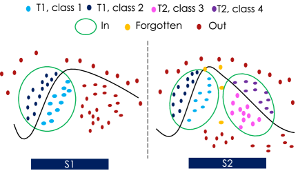
Figure 1: Illustration of three three different sets of samples constructed in the context of continual learning.

We divide the set of inspected samples into three subsets: (In) samples covering those of previously and recently learned concepts, (Forg) forgotten samples subject to mistaken predictions as a result of continual learning and, finally, the (Out) samples, covering those of yet unseen concepts. Our key goals are to understand (a) the existing novelty detection methods behaviour in this setting; (b) whether novelty detection methods are capable of coping with a dynamic (In) set; (c) how potentially forgotten samples are treated by the novelty detection methods. To this end, we propose a benchmark to evaluate several existing novelty detection methods.

We note a clear connection between continual learning and novelty detection and insights that novelty detection methods can provide about a continual learner’s behaviour and vice versa. We also highlight the need for developing new novelty detection methods that are closely linked to the trained model and the deployed continual learning method.
Our contributions are as follows:1) we are the first to investigate the novelty detection problem under the continual learning setting (3); 2) we establish benchmarks for the described continual novelty detection problem and compare different existing methods (4); 3) To stimulate research on this problem, we highlight possible promising directions and propose simple yet effective baselines (A.7).

2 Related Work

Our work lies at the intersection of continual learning, novelty detection and open world recognition. The main challenge faced by the continual learning methods is “the catastrophic” forgetting of previously learned information as a result the new learning episodes. Over the past years, solutions have been proposed for different settings: the multi-head setting (Aljundi et al., 2018; Lee et al., 2017; Kirkpatrick et al., 2017; Finn et al., 2017; Nguyen et al., 2017) where each new learning episode (representing a separate task) has a dedicated output layer, the shared-head setting (Rebuffi et al., 2017; Zhao et al., 2020; Wu et al., 2019; Hou et al., 2019) in which the learnt groups of classes at different episodes share the same, single output layer, and the online setting (Aljundi et al., 2019c; Lopez-Paz et al., 2017; Aljundi et al., 2019a) where learning happens online on a stream of data. We refer to Delange et al. (2021) for a survey. In this work, we consider multi-head and shared-head settings. Further, continual learning methods assume that new classes arrive in batches along with their labelled data while at test time only learned classes are assumed to be present. Very recently, methods were proposed to detect task boundaries (Lee et al., 2020; Zeno et al., 2018; Aljundi et al., 2019b), i.e., when a new task different from the existing training data is encountered. However, this detection assumes that samples of new tasks are received in batches along with their labels and mostly rely on the statistics of the loss function for such detection.
Novelty Detection or Out of distribution detection (OOD) methods (Simonyan & Zisserman, 2014; Hendrycks & Gimpel, 2016; Liang et al., 2018; Hsu et al., 2020; Bodesheim et al., 2015; Schultheiss et al., 2017) tackle the problem of detecting test data that are different from what a model has been trained on. The detection is done offline where it is assumed that In distribution is final. Moreover, evaluation benchmarks don’t usually consider novel objects of similar input domain. Note that OOD approaches are also concerned with detecting adversarial attacks, however, in this work we are mainly interested in detecting relevant novel objects and not random input or adversarial attacks.
Open World Recognition describes the general problem of learning, identifying unknowns and the novel data that should be labelled and added to the existing training set, where new training steps can be performed (Bendale & Boult, 2015). Open world problems typically assume that the test examples which are identified as novel, are then labelled by an expert and used in new learning episodes. However in many scenarios labels are not available for these examples. In this work, data corresponding to the new learning steps are independent of the novelty detection results. Boult et al. (2019) have critically reviewed open world methods demonstrating unsuitably for deep neural networks. To the best of our knowledge, more recent works on open world for classification are very scarce. There is only one extension of (Bendale & Boult, 2015), to deep networks (Mancini et al., 2019) and an improved version (Fontanel et al., 2020) for web aided robotics applications, where training data are extracted from the web. This method simply relies on the nearest class mean distance for detecting novel input. Existing novelty detection methods for classification problems have not been evaluated out of the offline batch setting which is the aim of this work. With regards to the object detection problem, the open world detection methods (Joseph et al., 2021; Yang et al., 2021) are specific to object detectors where background class and multiple instances per image are essential in their formulation, hence not applicable to the general novelty detection problem for classification. These few works lack a proper validation of the novelty detection aspect and focus on the performance and accuracy of the learned classes under the open world setting. Moreover, in the few existing open world works, there is no specific use or discussion of possible continual learning methods, usually a simple stack of previous samples or their features is used to prevent catastrophic forgetting. As such, an evaluation of existing continual learning and novelty detection approaches in such setting is still missing. In summary, the existing few works of open world lack a proper consideration of the main continual leaning challenge, catastrophic forgetting, and how it affects the novelty detection performance. Whilst the open world setting is certainly interesting, we believe it is a complicated problem to start with, given the current state of continual learning and novelty detection. Differently, in this work instead of attempting at solving the whole open world problem at once, we start with the first essential step of studying how novelty detection can be extended to a continual learning scenario.
Given the recent efforts and advances in continual learning: We study how deploying a continual learning method to facilitate learning while preventing catastrophic forgetting affects the performance of existing novelty detection methods. Under this setting, we define 3 sets that emerge from the continual learning process (In, Out and Forg.) We study novelty detection methods behaviour under various continual learning settings with and without example replay, different architectures and different benchmarks.

3 Problem Description

We consider a continual learning scenario where batches of labelled data arrive sequentially at different points in time. Each new batch corresponds to a new group of categories that could form a separate task $\mathcal{T}_{t}$. Given a backbone model $\mathcal{M}$ e.g., a deep neural network, data arriving at time $t$ will be learnt in a stage $S_{t}$ updating the model status from $\mathcal{M}_{t-1}$ to $\mathcal{M}_{t}$, learning at stage $S_{t}$ will generally affect performance on all previous tasks $\mathcal{T}_{1}\cdots\mathcal{T}_{t-1}$. Acquired knowledge will be accumulated and updated across time and access to previously seen data is prohibited or limited. To prevent catastrophic forgetting of previously acquired knowledge, a continual learning method is applied during learning while maintaining a low memory and computational footprint. In between learning stages, the model will be deployed in a given test environment and should perform predictions on input covered by its acquired knowledge while identifying irrelevant input. A continual novelty detection method $\text{ND}(\mathcal{M}_{t})$ should be able to tell after each learning stage $S_{t}$ how familiar and similar a given input is to the current model $\mathcal{M}_{t}$ knowledge. The detection is carried online given each input. Following existing novelty detection methods, the output of a ND method is a score $sc$ that is higher for In distribution samples than for Out of distribution samples. Later on, novel inputs can be gathered and annotated, or other data can become available for training the model “continually” in a new learning stage $S_{t+1}$.

$\text{ND}(\mathcal{M}_{t})$ should reflect the incurred change as $\mathcal{M}_{t-1}$ transition to $\mathcal{M}_{t}$ expanding the set covered by the trained model to contain samples of the previous and the current learning stages. Further, as forgetting of previous knowledge can occur, we want firstly to understand how forgotten data are treated by the ND method and also examine what the novelty detection behaviour could tell about the continual learning. For that purpose, after each stage $S_{T}$, we divide the test data into three sets:

• In: Samples that are represented by the current training stage or those from previous stages whose predictions remain correct (i.e., not forgotten). As in Hendrycks & Gimpel (2016) the In set contains only correctly predicted test samples.

  $$In_{t}=\{x:x,y\sim D^{k}_{x,y}\wedge k\in[1..t]\wedge\mathcal{M}_{t}(x)=y\}$$ (1)

• Out: Samples of unknown tasks, classes or domains that are not covered by the current model, this set contains samples that could be covered in the future.

  $$Out_{t}=\{x:x,y\sim D^{k}_{x,y}\wedge k\notin[1..t]\}$$ (2)

• Forg: Samples of previously learned stages that were predicted correctly and are predicted wrongly now.

  $$Forg_{t}=\{x:x,y\sim D^{k}_{x,y}\wedge k\in[1..t-1]\wedge\mathcal{M}_{t}(x)\neq y\wedge\mathcal{M}_{k}(x)=y\}$$ (3)

  Forgetting is an essential phenomena when training models incrementally, within this work, we aim at understanding how this phenomena affects novelty detection methods. Hence, we construct the Forg set, to examine how forgotten samples are treated by a ND method, as Out or In, or if forgotten samples can be potentially identified as a separate set e.g., with a score lower than In and higher than Out, $sc$(In)$>sc$(Forg)$>sc$(Out). If identified, those samples can be further utilized to update the model, recovering previous important information.

Note that all sets are constructed from test data not seen during the different training stages. Figure 1 illustrates how these sets are constructed during continual learning.

4 Empirical Evaluation of Existing methods

4.1 Datasets

In order to evaluate existing ND methods in the setting of CL, we construct the following learning sequences that are commonly used to evaluate state of the art CL methods:
1) TinyImageNet Sequence: a subset of 200 classes from ImageNet (Stanford, ), rescaled to size $64\times 64$ with 500 samples per class. Each stage represents a learning of a random set of 20 classes composing 10 stages (Delange et al., 2021). Here, all training stages data belong to one dataset in which no data collection artifacts or domain shift can be leveraged in the detection;
2) Eight-Task Sequence: Flower (Nilsback & Zisserman, 2008) $\rightarrow$ Scenes (Quattoni & Torralba, 2009) $\rightarrow$ Caltech USD Birds (Welinder et al., 2010) $\rightarrow$ Cars (Krause et al., 2013) $\rightarrow$ Aircraft (Maji et al., 2013) $\rightarrow$ Actions (Everingham et al., ) $\rightarrow$ Letters (de Campos et al., 2009) $\rightarrow$ SVHN (Netzer et al., 2011). The samples of each task belong to a different dataset and each task represents a super category of objects. This CL sequence has been studied in (Aljundi et al., 2018; Delange et al., 2021) under the multi-head setting.

TinyImageNet

Eight-Task Seq.

Setting

Shared-head

Multi-head

Multi-head

Architecture

ResNet

ResNet

VGG

AlexNet

CL Method

ER 25s

ER 50s

SSIL 25s

SSIL 50s

LwF

MAS

FineTune

LwF

MAS

FineTune

LwF

MAS

FineTune

Acc. $\uparrow$

$26.20\%$

$32.09\%$

$31.26\%$

$33.02\%$

$69.39\%$

$61.59\%$

$37.97\%$

$61.7\%$

$53.94\%$

$32.66\%$

$50.95\%$

$50.26\%$

$29.51\%$

Forg. $\downarrow$

$24.72\%$

$14.2\%$

$15.6\%$

$15.02\%$

$3.5\%$

$2.01\%$

$36.47\%$

$4.01\%$

$9.37\%$

$37.54\%$

$5.0\%$

$2.90\%$

$26.38\%$

Table 1: CL Average Accuracy and Average Forgetting at the end of the training sequence for each considered setting with different continual learning methods. Finetune forgets catastrophically, MAS is more conservative but less flexible compared to LwF. SSIL improves over ER in the low buffer regime.

4.2 Continual Learning Setting

In this work, we consider the setting where training data of each stage $S_{t}$ is learnt offline with multiple epochs. In the context of image classification, we study both multi-head and shared-head settings explained in the sequel.
Multi-head setting. Data of each learning stage $S_{t}$ is learnt with a separate output layer (head). It is largely studied and it is less prone to interference between tasks as the last output layer is not shared among the learned tasks. However, knowledge of the task identity is required at test time to forward the test sample to the corresponding output layer. In order to limit forgetting, we train the prediction model with a CL method. We use two well established methods from two different families: Learning without Forgetting (LwF) (Li & Hoiem, 2016) uses the predictions of the previous model $\mathcal{M}_{t-1}$ given the new stage $S_{t}$ data to transfer previous knowledge to the new model $\mathcal{M}_{t}$ via a knowledge distillation loss. Memory Aware Synapses (MAS) (Aljundi et al., 2018) estimates an importance weight of each model parameter w.r.t. the previous learning stages. An L2 regularization term is applied to penalize changes on parameters deemed important for previous stages. These methods are lightweight, require no retention of data from previous tasks and are well studied in various CL scenarios. We also evaluate a fine-tuning baseline that does not involve any specific technique to reduce forgetting, we refer to this as FineTune. Note that multi-head setting requires at test time a “task oracle” to forward the test data to the corresponding head.
Shared-head setting. Here, the last output layer is shared among categories learned at the different stages. This is a more realistic setting, however prune to severe forgetting of previous tasks. As such, most approaches use a buffer of a subset of previously seen samples. We study shared-head continual learning with a fixed buffer of different sizes corresponding to 25 samples per class and 50 samples per class as in Delange et al. (2021). We consider two continual learning methods: Experience Replay (ER) (Rolnick et al., 2018) where buffer samples of previous classes are simply replayed while learning new classes and Cross Entropy loss is minimized on replayed and new samples together at each iteration. Separated Softmax for Incremental Learning (SSIL) (Ahn et al., 2021) where a Softmax and task wise knowledge distillation are applied to each task logits separately in order to reduce the interference with previous tasks logits activations.
Architecture. We consider three different backbones, ResNet and VGG for TinyImageNet Seq.. For the Eight-Task Seq., we use a pretrained AlexNet model as in Delange et al. (2021); Aljundi et al. (2018).
Training details. For CL, early stopping on a validation set was used at each learning stage. Following Mirzadeh et al. (2020) an appropriate choice of regularization and hyperparameters could lead to a stable SGD training resulting in smaller degrees of forgetting. Hence, we use SGD optimizer where dropout, learning rate schedule, learning rate, and batch size were treated as hyper-parameters. Since our goal is to study the behaviour of ND methods in a CL scenario, we chose CL hyper-parameters that achieve the best possible CL performance, in order to reduce any possible effect of negative training artifacts on the ND performance. Thus, our CL results might be higher than those reported in Delange et al. (2021). Training was performed over ten random seeds and mean accuracy and forgetting are reported.

4.3 Novelty Detection Setting

Deployed ND methods. For novelty detection, a method should be able to perform prediction given an input data point and a model. We do not consider methods that require simultaneous access to the training data due to the continual learning scenario under consideration. We select four different ND methods covering different detection strategies. 1) Softmax the output probability of the predicted class (an image classification scenario) after a softmax layer is used as a score for samples of the In set (Hendrycks & Gimpel, 2016). 2) ODIN (Liang et al., 2018) adds a small perturbation to the input image and uses the probability of the predicted class after applying temperature scaling as a score. 3) Mahalanobis (Lee et al., 2018) estimates the mean of each class and a covariance matrix of all classes given training data features. The Mahalanobis distances of different layers features are used by a linear classifier to discriminate In vs. Out samples. The covariance matrix and the mean are updated when new classes are added. 4) density models have been proposed as a way to perform OOD and we pick deep generative model trained as a VAE (An & Cho, 2015) as an example. Note that in the context of continual learning, the VAE itself is prone to catastrophic forgetting (Nguyen et al., 2017). We treat the choice of VAE input (raw input or features of the model’s last layer before classification) as a hyper parameter.

(a)

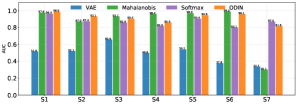
(b)

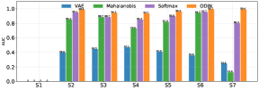
(c)

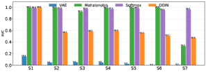
(d)

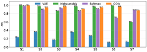
(e)

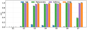
(f)

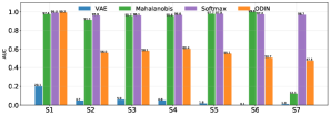
(g)

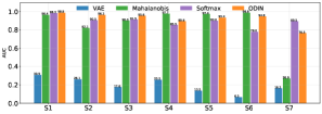
(h)

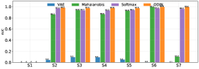
(i)

Figure 2: Novelty detection results for Eight-Task Seq. in terms of Combined  AUC (C.AUC), Recent stage AUC (R.AUC) and Previous stages AUC (P.AUC)  with FineTune  first row, MAS second row  and LwF  third row.

Evaluation. After each stage $S_{t}$ in the learning sequence, we evaluate the ND performance on the following detection problems constructed from the three sets mentioned earlier:
In / Out: It serves to examine the detection ability of samples from unseen categories (Out) vs. samples of learned categories. Note that the In set is changing after each learning stage to contain correctly predicted test samples from all the learning stages. Here Out contains test samples classes that are yet to be encountered in the continual learning sequence. Hence the novelty detection evaluation is carried on until stage $T$-$1$ where $T$ is the length of the sequence.
In / Forg & Forg / Out : We want to examine if the forgotten samples are treated as novel, similarly to those in the Out set. In other words, can an ND method discriminate between a forgotten sample and a correctly predicted one? Moreover, does the predicted score for Out differ from that of Forg. Ideally, if an ND method could tell if a sample is forgotten rather than completely novel, those identified samples can later be treated differently either in the way they are re-annotated or re-learnt by the model.

Metrics. We consider the following metrics: AUC: Area Under the receiver operating Characteristic curve (Hendrycks & Gimpel, 2016). It can be interpreted as the probability that an In sample has a greater score than an Out sample.
AUPR-IN: Area Under the Precision Recall curve where In samples are treated as positives (Hendrycks & Gimpel, 2016). Detection Error (DER): The minimum possible detection error (Liang et al., 2018).
To examine closely the CL effects and how In samples belonging to previous learning stages are treated compared to those of the most recent stage of learning, we propose the following metrics: 1) Combined AUC (C.AUC), measures the novelty detection performance for all In samples regardless of the activated head, this is to check if the predicted scores differ across tasks, 2) the most Recent stage AUC (R.AUC), only concerned with In samples of the latest stage, 3) the Previous stages AUC (P.AUC) where In represents only data relevant to previous stages. For each ND method we tune the hyper-parameters based on an out of distribution dataset, namely CIFAR-10.

4.4 Results

4.4.1 Continual Learning Results

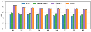
(a)

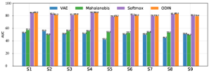
(b)

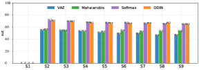
(c)

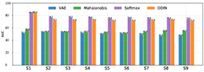
(d)

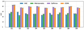
(e)

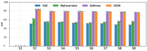
(f)

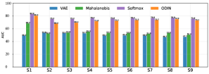
(g)

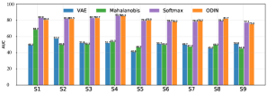
(h)

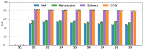
(i)

Figure 3: Novelty Detection results in terms of Combined  AUC (C.AUC), Recent stage AUC (R.AUC) and Previous stages AUC (P.AUC) for TinyImageNet Seq. with FineTune  first row, MAS  second row, and LwF  third row.

We first report CL methods performance in order to note the methods’ behaviour in the studied settings and lay the ground for a better understanding of the ND methods performance in the different cases. Table 1 reports the CL performance in terms of average accuracy and average forgetting at the end of each learning sequence under different settings. In the Appendix, we report each task performance.
MAS applies a regularization term directly to the network parameters, penalizing their changes. As such, in general, MAS is more conservative than LwF and tends to largely preserve the performance of the very first learned classes. However the later stages struggle in the learning process, failing to reach the expected performance of each task. For LwF no direct constraints are applied to the parameters but knowledge distillation is deployed on the network output giving the later learning stages flexibility in steering the parameters towards a better minimum. As such, LwF shows lower accuracy on classes encountered in the early stages and larger forgetting but higher accuracies on the later. LwF performs best especially in TinyImageNet Seq.. FineTune does not control forgetting, resulting in a low performance on previous stages and best performance on the most recent one. For shared head settings, in general larger forgetting rates are shown as a result of the shared output layer. The larger the deployed buffer, the higher the previous tasks performance and the smaller the forgetting. SSIL  succeeds in reducing tasks interference and hence forgetting compared to ER  especially when a small buffer is deployed.

4.4.2 Novelty Detection Results

Having discussed the continual learning performance across different sequences and different methods, here we study the obtained novelty detection performance and how the shown differences in the made CL tradeoffs affect the ND methods performance.
Eight-Task sequence ND results. Figure 2 shows the ND performance based on the AUC metric for the Eight-Task Seq. with FineTune (first row), MAS (second row) and LwF (third row). Due to space limit, performance based on other metrics is shown in  the Appendix. In each row, we show three sub figures: Combined AUC (C.AUC), the current stage AUC (R.AUC) and the previous stages AUC (P.AUC). The achieved novelty detection performance is particularly high for ODIN and Softmax, which leverage directly the multi-head nature by relying on the predicted class probability. For Mahalanobis, that operates in the learned feature space and hence does not leverage the separate output layers, the most recent task performance remains high through the sequence while the previous tasks AUC fluctuates as different tasks are being seen, possibly linked to the various degree of relatedness among the learned tasks since the Out set is composed of yet to be seen tasks samples. Note that for Mahalanobis the mean and covariance estimated on previous tasks remain unchanged and hence might be outdated when significant changes happen on the features. Moreover, in this sequence, the last task is SVHN that is visually similar to its precedent Letters, which explains why the ND performance of the last stage is lower than previous ones. While VAE has a reasonable performance on the first learned task, it rapidly drops as more tasks are learnt due to catastrophic forgetting in the VAE itself. It is worth noting that, the AUC of the first task is high for the Out sets belonging to the next 4 tasks. However for the last 3 tasks of Action, SVHN, Letter VAE fails to identify their samples as Out. On another note, ODIN performance seems the best on the R.AUC and P.AUC metrics, nevertheless, on C.AUC it is lagging behind Softmax and Mahalanobis, indicating that the predicted novelty scores heavily rely on the used output head.

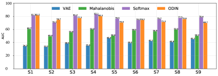
(a)

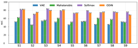
(b)

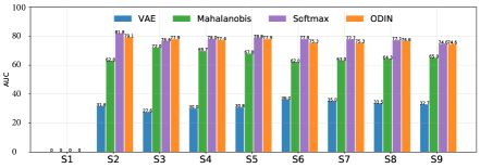
(c)

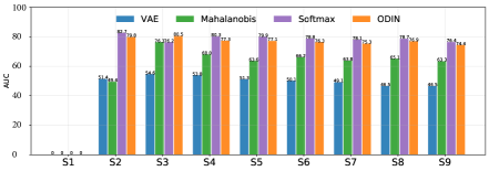
(d)

Figure 4: First row shows current stage  (R.AUC), second row shows previous stages (P.AUC) for TinyImageNet Seq. with  ER  under shared head setting with two different buffer sizes, 25 samples and 50 samples per class.

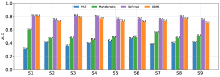
(a)

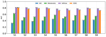
(b)

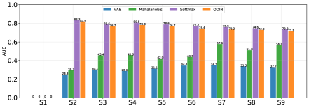
(c)

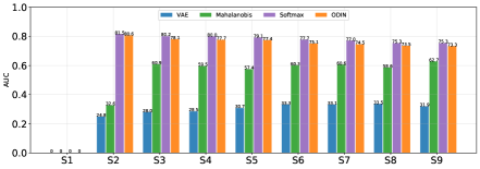
(d)

Figure 5: First row shows current stage  (R.AUC), second row shows previous stages (P.AUC) for TinyImageNet Seq. with  SSIL  under shared head setting with two different buffer sizes, 25 samples and 50 samples per class.

TinyImageNet sequence. Here we examine ND methods performance on TinyImageNet Seq. where new categories are learnt with no shifts in the input domain. Figure 9 shows the C.AUC, R.AUC and P.AUC for FineTune (first row), MAS (second row), LwF (third row).
We make the following observations. First, the overall ND performance of all methods is lower than the Eight-Task Seq., demonstrating the difficulty of this scenario. With FineTune, the R.AUC score is quite similar at the different stages in the sequence. However, the P.AUC score declines as new classes are learnt and it is significantly lower than the R.AUC. With MAS and LwF aiming at reducing catastrophic forgetting, P.AUC scores of ND methods are significantly higher than for FineTune. For example, Softmax P.AUC is $75\%/77\%$ for MAS / LwF at the last evaluation stage compared to $64\%$ with FineTune. Second, the R.AUC scores with MAS / LwF are generally lower than with FineTune (R.AUC $74\%/77\%$ compared to $80\%$ with FineTune). This indicates that, while preserving the performance on previous classes, the current stage suffers learning difficulties, translated into a decline in the ND performance. Another manifestation of the famous stability/plasticity dilemma. With LwF, the R.AUC scores seem slightly better than MAS, which is indicative of the ability of LwF to adapt more to the new learning stage and to leverage the benefits of transfer learning, especially when the learned classes are similar.
When examining the different ND methods performance we can note the following: the simplest method Softmax performs the best especially in the C.AUC, ODIN has consistently lower C.AUC score than Softmax, as also seen in the Eight-Task Seq. evaluation. For Mahalanobis and VAE, the performance is considerably worse than methods operating on the output layer probabilities (ODIN and Softmax). Note that by operating directly on the output probability they benefit from the CL method, while Mahalanobis and VAE suffer from the CL constraints. In the Appendix ND experiments are shown with VGG as a backbone model. Similar trends can be noted, our observations seem to be independent of the deployed backbone.

Overall, in spite of the fact that the In sets are constructed only from correctly predicted samples, a clear degradation in ND performance can be seen as more learning steps are carried. Our results show that the quality of the learning and the characteristic of the continual learning method affect directly the performance of the novelty detection method.

low DER $<20$

medium DER $>20~{}\&<35$

high DER $>35$

Setting	Method	$S_{2}$		$S_{T-1}$		$S_{T}$
		F. vs. N.	F vs. O.	F. vs. N.	F vs. O.	F. vs. N.
Eight-Tasks FineTune	Softmax	19.2	17.5	33.5	35.3	36.6
	ODIN	32.5	7.6	35.7	4.2	36.9
	Mahalanobis	49.9	16.8	49.1	46.6	49.4
	VAE	50.0	50.0	48.8	50.0	49.5
Eight-Tasks MAS	Softmax	7.6	12.4	21.3	14.6	22.3
	ODIN	26.9	3.2	31.6	2.1	31.2
	Mahalanobis	49.9	10.2	48.4	38.2	11.8
	VAE	49.8	50.0	48.8	50.0	49.0
Eight-Tasks LwF	Softmax	15.4	15.3	20.0	16.2	24.7
	ODIN	30.7	10.5	33.1	1.3	35.0
	Mahalanobis	49.8	19.7	48.8	49.9	43.3
	VAE	49.8	50.0	48.8	50.0	49.0
TinyImag. Seq. FineTune	Softmax	31.3	48.3	35.6	49.4	36.4
	ODIN	33.9	46.7	36.5	49.3	36.2
	Mahalanobis	44.8	46.2	45.9	48.0	45.5
	VAE	46.7	47.6	47.2	47.9	46.7
TinyImag. Seq. MAS	Softmax	15.4	49.7	18.9	48.6	16.3
	ODIN	24.4	48.0	29.0	47.0	27.0
	Mahalanobis	42.9	43.8	43.2	44.4	43.0
	VAE	46.7	47.6	47.2	47.9	46.7
TinyImag. Seq. LwF	Softmax	20.6	49.5	8.5	48.3	17.9
	ODIN	24.2	49.4	26.6	46.1	26.5
	Mahalanobis	45.7	46.0	43.2	47.8	44.9
	VAE	46.7	47.6	47.2	47.9	46.7
TinyImag. Seq. ER 25s	Softmax	21.3	46.3	30.6	46.5	30.8
	ODIN	29.6	40.3	32.3	45.5	32.1
	Mahalanobis	37.5	46.1	39.4	47.0	38.5
	VAE	45.3	45.1	47.2	48.6	46.8
TinyImag. Seq. ER 50s	Softmax	19.9	46.4	27.3	46.9	29.5
	ODIN	28.2	45.5	32.4	45.2	31.9
	Mahalanobis	47.3	43.8	40.0	45.4	39.3
	VAE	45.3	45.1	47.2	48.6	46.8
TinyImag. Seq. SSIL 25s	Softmax	27.7	43.1	32.9	42.1	33.0
	ODIN	30.7	38.9	38.0	39.1	37.2
	Mahalanobis	49.1	49.6	45.5	48.4	447.1
	VAE	45.3	48.6	49.0	44.6	47.3
TinyImag. Seq. SSIL 50s	Softmax	24.0	46.3	30.7	39.6	34.1
	ODIN	28.7	41.5	36.4	37.9	38.3
	Mahalanobis	49.1	48.4	46.4	48.0	42.3
	VAE	49.9	49.1	48.5	49.2	49.2

Table 2: Detection errors ($\%$) of Forg (F) vs. In (N) and Forg (F) vs. Out (O) in the studied settings. Due to space limits, we only show the first and the last two stages demonstrating the change. Colors are used to highlight the change across the sequence. In the Appendix, we report all stages and other metrics.

Shared-head results. We move to a setting where some previously seen samples are maintained and a shared output layer is used for all the learned classes.
Figures 4 and  5 show the R.AUC and the P.AUC metrics, with ER  and  SSIL  respectively for different buffer sizes. We do not report the C.AUC as this is a shared-head setting. The further in the sequence, the more the P.AUC scores decline, although a larger buffer mitigates this effect. In the Appendix, we show the performance on each In set at the different learning steps. It can be noticed that even when a replay buffer is used, novelty detection performance on the first learning stage is the highest among all other stages. In the Appendix, we show that the AUC of the first In set is higher than the second In set and the gap increases with increasing the deployed buffer size. This indicates difficulties with learning the new data while maintaining the performance on replayed samples. This is the case for both CL methods, ER  and SSIL.
On the ND methods performance, in general, ODIN R.AUC scores here are lower than Softmax. However, the P.AUC scores for ODIN and Softmax are quite similar. For Mahalanobis, although it does not leverage the replay buffer, better performance with ER  is shown compared to multi-head setting, indicating a better feature preservation. This could suggest that larger rates of forgetting and shift in the features space might be hidden in the multi-head setting.
However when SSIL  is used as a CL method, Mahalanobis performance is close to random and ODIN performance is consistently lower than Softmax. We hypothesize that the focus on the preservation of the Softmax probabilities in  SSIL  comes at a cost of a weaker features reservation.

General observations. We highlight the following points on all the studied settings: 1) The further in the sequence, the worse is the ND performance. The incremental nature of the learning and the suffered forgetting affect even the correctly predicted samples and the way they are represented. 2) ND methods also need a mechanism to control forgetting. What is captured by the ND method of old data can be outdated as a result of the continuous model’s updates, hence unless the ND method uses directly the model output, its performance radically drops. 3) Softmax the simplest method works best. In spite of being the beaten baseline in the typical ND benchmarks, using the predicted class probability outperforms more complex choices. However, a large gap remains between the ND performance in the TinyImageNet Seq. and that of OOD benchmarks suggesting a big room for improvements. 4) ND performance on the “first” stage data is better than later stages. The first stage is learnt alone, while other stages are performed under constraints to prevent forgetting, and for shared-head setting the reminder of the classes (when first learned) have to be discriminated from already well learned classes. Such bias hinders the learning in the later stages.

What happens to the forgotten samples? We want to examine how forgotten samples are treated by the ND method. Since those samples belong to a previous In set, are they treated similarly to the other In samples that are correctly predicted? Or are they now considered by the ND method as Out samples? Can a novelty detection method possibly identify the In vs. Forg vs. Out? Table 4 reports the detection error (DER) of In vs. Forg and Forg vs. Out in the different settings. First of all, similar to previous observations, it can be seen that in later learning stages, the detection errors get higher. For the Eight-Task Seq., forgotten samples can be easily discriminated from unseen task samples (Forg vs. Out). This is the case mostly for ODIN, Softmax and Mahalanobis. It indicates a difference in the output probability and the feature distribution between Forg and Out. Note that the Out samples belong to completely different tasks in this sequence. However, in all other cases, it is extremely hard to discriminate samples of Out sets from Forg set. Does it mean that those are treated similarly? If we look closely, ODIN is constantly better in all cases than Softmax suggesting that the perturbation added to the input affects more Out samples than Forg samples. This could provide a direction on how the separation of Forg samples from Out samples could be approached.
Regarding In vs. Forg, we can see that while at the second stage the detection error might be reasonable and those two sets can be differentiated, as new learning stages are carried the detection gets harder. It is also worth noting that only methods that utilize the output probability could tell the difference, as opposed to those that operate in the feature space, such as Mahalanobis, suggesting that forgetting at first is more present at the output layer. For TinyImageNet Seq., the multi-head setting with a dedicated CL method (MAS or LwF), shows clearly better detection performance of In vs. Forg for Softmax and ODIN when compared to FineTune. Finally, the shared head setting poses the most challenging detection of Forgotten samples. In spite of SSIL showing better CL performance than ER,  Forg  samples are harder to discriminate from In samples when SSIL is deployed compared to ER. Overall, we believe that the study of the novelty detection in the continual learning scenario brings extra insights on the learning characteristics that might be hidden when looking merely at the continual learning performance.

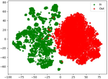
(a)

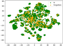
(b)

(c)

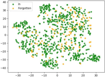
(d)

Figure 6: tSNE 2D visualization. (a) and (c) show the projection of IN and Out samples based on $\mathcal{M}_{1}$, (b) and (d) show the sets of IN and Forg based on $\mathcal{M}_{2}$ for multi-head TinyImageNet Seq. and Eight-Task Seq..

5 Discussion and Additional Baselines

tSNE visualization. With the goal of understanding how the features of the 3 sets are distributed and whether this relates to the nature of the sequence (disjoint tasks vs. different groups of classes), we examine the 2D tSNE projections of the (In, Out, Forg). Figure 6 shows the tSNE projections of the first (In, Out, Forg) sets for Eight-Task Seq. and multi-head TinyImageNet Seq. based on the last layer features. It can be seen that in the later case, the Out samples are projected in between the different clusters of learned categories as opposed to the Out set, being a different dataset, and thus a different domain. This might explain the low ND performance in TinyImageNet Seq. compared to Eight-Task Seq.. In both settings, the forgotten samples appear on the boundaries of a predicted category cluster after a movement from one cluster to another that possibly caused mistaken predictions (forgetting).
A similarity based view.  Boudiaf et al. (2020) shows that the optimal weights of the last classification layer are proportional to the features mean. Similar analogies between the last layer class weights and the class feature mean are made in Lee et al. (2018); Qi et al. (2018). In continual learning, access to old data can be prohibited but the learned features of all categories are frequently updated. As such, we propose to exploit the analogy between the learned classes weights and the features, and treat the last layer class weights as prototypes of the learned classes. Instead of solely relying on the predicted class probabilities, we can directly leverage the similarities of an input sample to different class prototypes. We consider a neural network with no bias term in the last layer. Consider an input sample $x$ and a neural network $\{\phi,\theta\}$ with $\phi$ the feature extraction layers and a fully-connected final classification layer represented by $\theta\in\mathbb{R}^{k\times n}$, where $n$ is the dimensionality of features $\phi(x)$ and $k$ is the number of classes. The $i^{\text{th}}$ column of $\theta$ is denoted as $\theta_{i}$. The network output before the softmax is $\phi(x)\theta^{\intercal}$ and the predicted class satisfies $c=\operatorname*{arg\,max}_{i}(\phi(x)\cdot\theta_{i})=\operatorname*{arg\,max}_{i}(\|\phi(x)\|\|\theta_{i}\|\cos(\alpha_{i}))$, where $\alpha_{i}$ is the angle between $\phi(x)$ and $\theta_{i}$. The norm of an extracted feature $\phi(x)$ and the cosine of the angle between $\phi(x)$ and the most similar class are data-dependent terms i.e., the scalar projection of $\phi(x)$ in the direction of $\theta_{c}$. In the Appendix, we investigate statistics of $\phi(x)$ (mean, std., norm) for the studied sets at different stages. We note that after the first stage, the feature norm of In is significantly larger than that of Out. However, in the later learning stages the difference disappears. This might be a possible cause for the degradation of Softmax performance in the later stages. Particularly, Forg samples show low features norm compared to In samples. In the following, we suggest two additional baselines leveraging the similarities between the features and the class prototypes.
Baseline 1. Given an input $x$, the estimated class probability vector is $p_{x}=[p_{x}^{1},p_{x}^{2},\dots,p_{x}^{k}]$, with $p_{x}^{c}=\frac{e^{\phi(x)\cdot\theta_{c}}}{\sum_{i}{e^{\phi(x)\cdot\theta_{i}}}}$. We hypothesize that In samples can be better explained by the class prototypes than those of Out samples. We thus estimate vector $z=p_{x}\theta^{*}$, where $\theta^{*}\in\mathbb{R}^{k\times n}$ is the matrix of normalized class prototypes. Denoting the normalized sample feature by $\phi^{*}(x)\in\mathbb{R}^{n}$, we define a scalar score $s=\phi^{*}(x)\cdot z$, which we refer to as B1 and use it for novelty detection. Note that $s$ is equal to the weighted sum of cosine similarities between $\phi(x)$ and the prototypes from $\theta^{*}$.
Baseline 2. To further exploit the features/prototypes similarities, we leverage the difference between the estimated similarities to the $(n)$ closest class prototypes. We suggest adding a perturbation to the features vector $\phi(x)$ corresponding to the gradient of the cross-entropy loss given a candidate class as a label. With $y_{n}$ being the $n^{\text{th}}$ closest class, the estimated gradient (perturbation) is $g_{n}=\nabla_{\phi(x)}\ell(\phi(x),y_{n})$ and the updated feature vector is $\phi^{\prime}_{x}=\phi(x)-g_{n}$. Then we estimate the difference $\Delta$ in the cosine similarity between the predicted class $c$ and the $n^{\text{th}}$ closest class as $\Delta=\cos(\alpha_{c})-\cos(\alpha_{n})$. We add this score to the score of B1 and refer to it as B2.

Setting	Method	m.P.AUC $\uparrow$	m.R.AUC$\uparrow$	mAUC$\uparrow$	F/IN$\downarrow$	F/Out$\downarrow$
Multi-head FineTune	Softmax	66.1	81.6	71.0	31.0	43.8
	B1	67.7	83.0	72.5	30.8	43.6
	B2	68.1	83.2	72.8	30.2	43.8
Multi-head MAS	Softmax	78.1	76.7	78.2	14.5	43.4
	B1	78.4	77.1	78.5	22.8	40.8
	B2	79.1	77.7	79.2	20.6	41.9
Multi-head LWF	Softmax	79.7	80.5	80.3	17.1	42.9
	B1	80.3	82.2	81.1	22.6	39.8
	B2	80.8	82.4	81.6	20.4	41.0
Shared-head ER-25s	Softmax	78.4	70.5	76.6	22.8	42.2
	B1	78.7	69.7	76.4	25.5	41.0
	B2	79.8	71.4	77.7	23.7	41.4
Shared-head ER-50s	Softmax	80.1	69.8	77.8	22.2	41.0
	B1	79.1	66.1	76.1	25.9	39.2
	B2	80.7	68.9	78.0	23.5	40.1
Shared-head SSIL-25s	Softmax	77.6	78.6	77.9	27.9	36.9
	B1	76.5	73.0	75.8	32.1	34.6
	B2	78.0	70.6	76.5	29.3	35.9
Shared-head SSIL-50s	Softmax	78.1	77.6	78.0	27.9	37.2
	B1	77.5	72.0	76.4	32.2	34.6
	B2	78.5	69.2	76.7	29.8	36.1

Table 3: ND performance (TinyImageNet Seq.) expressed in the mean of each measure $\%$  w.r.t. Softmax and our baselines (B1,B2).

Results. We retrained the models in TinyImageNet Seq. with no bias term and obtained similar CL performance, we refer to the Appendix for additional details and notes on the shared-head setting. Table 5 compares the ND performance of our proposed baselines to Softmax, the best studied method. Our baselines show better performance than Softmax in the different settings especially in the case of severe forgetting with FineTune. Our proposed baselines serve to stimulate investigating diverse directions. We believe that the ideal solution directly couples an ND module and a CL model, which could better exploit any discriminative patterns of the In set.

6 Conclusion

We introduce the problem of continual novelty detection, a problem that emerges when novelty detection techniques are deployed in a continual learning scenario. We divide the detection problem into three sub-problems, In vs. Out, In vs. Forg and Forg vs. Out. We examine several novelty detection techniques on these sub-problems in various continual learning settings. We show an increase in the detection error of In vs. Out as a result of continual learning. Surprisingly, the most simple ND method, Softmax, works best, yet poorly, in the studied settings opening the door for more sophisticated methods to tackle this challenging problem. When investigating how the Forg set is treated, it appears that as learning stages are carried, the confusion with In set increases. However, unless the Out set is composed of a different dataset, it is extremely hard for current ND methods to discriminate In from Forg. We present baselines improving over Softmax in an attempt to stimulate further research in this problem.

7 Ethics in Continual Novelty Detection

This work introduces the notion of applying novelty detection techniques in the setting of continual learning. As such, ethical implications of both aspects need to be pondered upon in this setting. Regarding novelty detection, the implications are rather positive, as it serves to bring more transparency to whichever knowledge has been embedded in the model. This, in turn, may help to alleviate biases introduced in the training set, or by the unbalanced nature of the data. As for the continual learning aspect of it, we show that the rate of samples that are forgotten as the model learns new tasks gets invariably larger. In our study, we assume that the different tasks share the same importance. However, we foresee the need for methods that are able to continually adjust the relative importance of each task. How this importance is assigned, and the nature of the tasks, may have ethical implications.

Appendix A Appendix

A.1 Introduction

In this appendix, we show the following: 1) For each continual learning method and under the different considered settings, we report each task Accuracy at the end of the sequence, Subsection A.2. 2) We report the novelty detection performance on TinyImageNet Seq. multi-head when using VGG as a backbone model, Subsection A.3. 3) We report the novelty detection performance with AUPR-IN and DER metrics, Subsection A.4. 4) We report the novelty detection performance on each In set before the last learning stage, Subsection A.5. 5) We report the full Forg vs. In and Forg vs. Out scores with different metrics, Subsection A.6. 6) We report statistics of the learnt features under the different settings, Subsection A.7.

A.2 CL Per Task Performance

In the main paper, we have reported the average accuracy and the average forgetting of the various CL settings and deployed methods. Here we report the average accuracy of each task at the end of the sequence for the different settings (Figures 7 & 8). These results support the discussions and the insights on the differences between MAS and LwF as different deployed continual learning methods. MAS is more conservative and tend to preserve the performance on the very first tasks while LwF is more flexible allowing more forgetting of the first tasks but obtaining better accuracy on average.

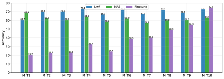
(a)

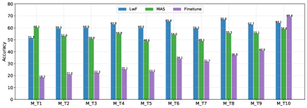
(b)

Figure 7: Seen tasks accuracy at the end of TinyImageNet Seq. with ResNet and VGG as backbones.

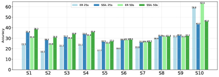
(a)

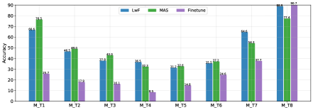
(b)

Figure 8: (a) Seen tasks accuracy at the end of TinyImageNet Seq. with ResNet as a backbone and shared-head setting. (b) Seen tasks accuracy at the end of Eight-Task Seq. with multi-head and AlexNet as a backbone.

A.3 ND Performance on Another Backbone.

In the main paper, we have reported the ND performance for TinyImageNet Seq. multi-head setting with only ResNet as a backbone model. Here, we report the ND performance when using VGG as a backbone model. Figures 9, 10, 11 report the Combined AUC (C.AUC), Recent Stage AUC (R.AUC) and Previous stages AUC (P.AUC) metrics for FineTune, MAS and LwF respectively. It can be seen that the ND performance deteriorates as more learning stages are passing, this is more severe when no continual learning method is applied (FineTune). Softmax and ODIN are the best methods, with Softmax performing best when looking at the Combined AUC (C.AUC) metric. We note that our observations are consistent for both backbones, ResNet and VGG.

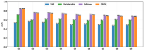
(a)

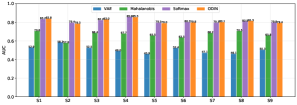
(b)

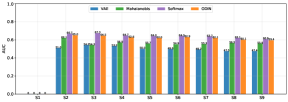
(c)

Figure 9: Novelty detection results in terms of Combined AUC (C.AUC), Recent stage AUC (R.AUC) and Previous stages AUC (P.AUC) for TinyImageNet Seq. with FineTune and VGG network as a backbone.

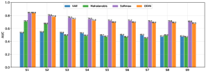
(a)

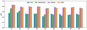
(b)

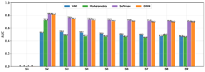
(c)

Figure 10: Novelty detection results in terms of Combined AUC (C.AUC), Recent stage AUC (R.AUC) and Previous stages AUC (P.AUC) for TinyImageNet Seq. with MAS and VGG network as a backbone.

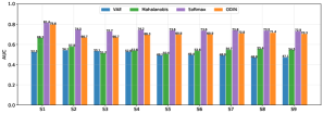
(a)

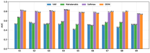
(b)

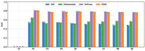
(c)

Figure 11: Novelty detection results in terms of Combined AUC (C.AUC), Recent stage AUC (R.AUC) and Previous stages AUC (P.AUC) for TinyImageNet Seq. with LwF and VGG network as a backbone.

A.4 Novelty detection Performance with Other Metrics

Here, we report the average DER and AUPR-IN scores of the In vs. Out detection problems at each learning stage. Figures 12, 13, 14, 15, 16 show the AUPR-IN scores for Eight-Task Seq., TinyImageNet Seq. multi-head with ResNet, TinyImageNet Seq. multi-head with VGG, TinyImageNet Seq. shared-head with ResNet and ER, shared-head with ResNet and SSIL  respectively. Figures 17, 18, 19, 20, 21 show the DER scores for Eight-Task Seq., TinyImageNet Seq. multi-head with ResNet, TinyImageNet Seq. multi-head with VGG, TinyImageNet Seq. shared-head with ResNet and ER, TinyImageNet Seq. shared-head with ResNet and SSIL  respectively.

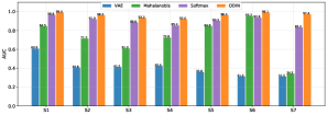
(a)

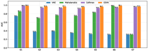
(b)

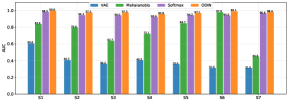
(c)

Figure 12: Novelty detection performance measured by AUPR-IN and estimated after each learning stage and averaged over all possible (In, Out) pairs, for Eight-Task Seq..

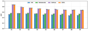
(a)

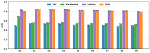
(b)

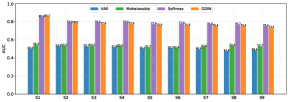
(c)

Figure 13: Novelty detection performance measured by AUPR-IN and estimated after each learning stage and averaged over all possible (In, Out) pairs, for multi-head TinyImageNet Seq. with ResNet.

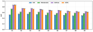
(a)

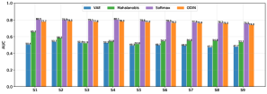
(b)

(c)

Figure 14: Novelty detection performance measured by AUPR-IN and estimated after each learning stage and averaged over all possible (In, Out) pairs, for multi-head TinyImageNet Seq. with VGG.

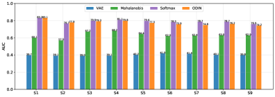
(a)

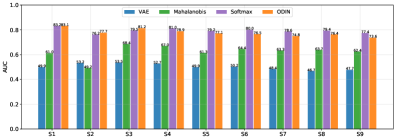
(b)

Figure 15: Novelty detection performance measured by AUPR-IN estimated after each learning stage and averaged over all possible (In, Out) pairs, for shared-head TinyImageNet Seq. with ResNet and ER.

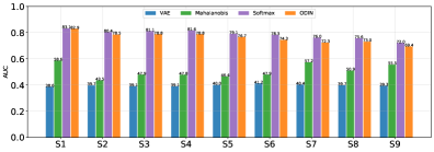
(a)

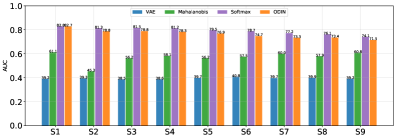
(b)

Figure 16: Novelty detection performance measured by AUPR-IN and estimated after each learning stage and averaged over all possible (In, Out) pairs, for shared-head TinyImageNet Seq. with ResNet and SSIL.

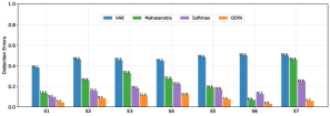
(a)

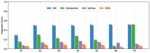
(b)

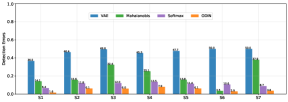
(c)

Figure 17: Novelty detection performance measured by DER (lower is better) after each learning stage averaged over each possible (In, Out) pair, for Eight-Task Seq..

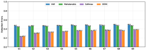
(a)

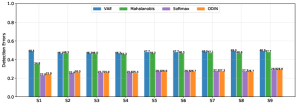
(b)

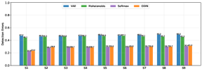
(c)

Figure 18: Novelty detection performance measured by DER (lower is better) after each learning stage averaged over each possible (In, Out) pair, for multi-head TinyImageNet Seq. with ResNet.

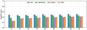
(a)

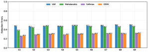
(b)

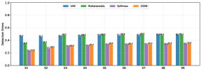
(c)

Figure 19: Novelty detection performance measured by DER (lower is better) after each learning stage averaged over each possible (In, Out) pair, for multi-head TinyImageNet Seq. with VGG.

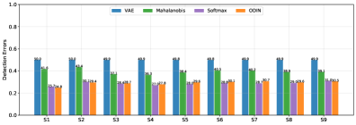
(a)

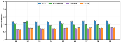
(b)

Figure 20: Novelty detection performance measured by DER performance after each learning stage averaged over each possible (In, Out) pair, for shared-head TinyImageNet Seq. with ResNet and ER.

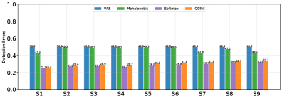
(a)

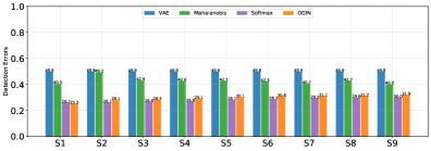
(b)

Figure 21: Novelty detection performance measured by DER performance after each learning stage averaged over each possible (In, Out) pair, for shared-head TinyImageNet Seq. with ResNet and SSIL.

A.5 Inspection of the ND Performance on Each In Set

In the main paper, we note that the ND performance could differ for the different considered In sets. Due to space limit, in the main paper we only report the Previous Stages (P.AUC) and the most Recent Stage (R.AUC) to discriminate between previously learnt sets and the newly learnt one. Here, we report the AUC score for each In set separately. To have an overall view, we consider the model before the last learning stage ($\mathcal{M}_{T-1}$) and we construct In sets for tasks or classes learnt at stages $1\dots T-1$ while the Out set represents the samples of the last task in the considered sequences. Figures 22, 23, 24, 25 show the last stage AUC for Eight-Task Seq., multi-head TinyImageNet Seq. and shared-head TinyImageNet Seq. (ER and SSIL) respectively. In most cases (except from LwF with TinyImageNet Seq.), the AUC scores of the first learnt In set remain higher than that for the consequently learnt In sets (i.e., at stage $2$ or $3$). This indicates that the isolated learning of the classes representing the first set was more stable leading to less forgetting rates compared to the later learnt classes.

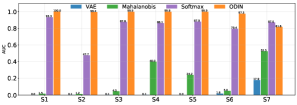
(a)

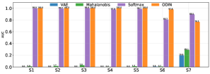
(b)

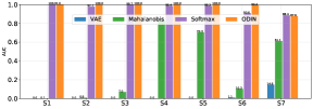
(c)

Figure 22: Novelty Detection Last Stage AUC. The AUC scores for each In set (learnt at each previous stage) vs. the last Out set based on the model before the last stag $\mathcal{M}_{T-1}$ for Eight-Task Seq..

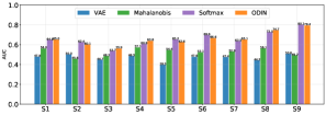
(a)

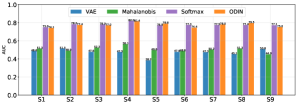
(b)

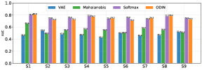
(c)

Figure 23: Last Stage AUC. The AUC scores for each In set (learnt at each previous stage) vs. the last Out set based on the model before the last stag $\mathcal{M}_{T-1}$ for multi-head TinyImageNet Seq. with ResNet.

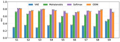
(a)

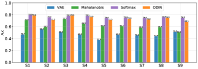
(b)

Figure 24: Last Stage AUC. The AUC scores for each In set (learnt at each previous stage) vs. the last Out set based on the model before the last stag $\mathcal{M}_{T-1}$ for shared-head TinyImageNet Seq. with ResNet with ER

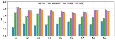
(a)

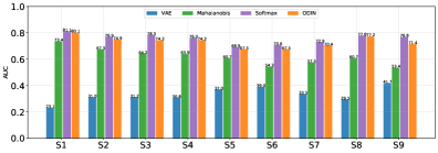
(b)

Figure 25: Last Stage AUC. The AUC scores for each In set (learnt at each previous stage) vs. the last Out set based on the model before the last stag $\mathcal{M}_{T-1}$ for shared-head TinyImageNet Seq. with ResNet with SSIL..

A.6 Forgotten Set (Additional Results)

In the main paper, due to space limit, we have shown the detection scores of Forg samples on 3 selected stages only. Here we show the full detection scores at all the different stages. Table 4 report the detection errors DER of In vs. Forg and Forg vs. Out at the different learning stages and under the different considered settings. Table 5 reports the AUC scores.

low detection error

medium detection error

high detection error

Setting	Method	M-S2		M-S3		M-S4		M-S5		M-S6		M-S7		M-S8		M-S9		M-S10
		F. vs. N.	F vs. O.	F. vs. N.	F vs. O.	F. vs. N.	F vs. O.	F. vs. N.	F vs. O.	F. vs. N.	F vs. O.	F. vs. N.	F vs. O.	F. vs. N.	F vs. O.	F. vs. N.	F vs. O.	F. vs. N.	F vs. O.
Eight-Tasks FineTune	Softmax	19.2	17.5	26.8	18.6	29.3	22.8	35.5	16.1	32.5	9.4	33.5	35.3	36.6	-	-	-	-	-
	ODIN	32.5	7.6	35.8	10.9	37.3	7.1	37.5	4.4	37.1	0.7	35.7	4.2	36.9	-	-	-	-	-
	Mahalanobis	49.9	16.8	47.7	39.5	49.3	19.0	49.7	12.0	49.3	4.9	49.1	46.6	49.4	-	-	-	-	-
	VAE	50.0	50.0	47.6	50.0	48.7	50.0	48.9	50.0	48.8	50.0	48.8	50.0	49.5	-	-	-	-	-
Eight-Tasks MAS	Softmax	7.6	12.4	12.1	15.5	15.0	9.8	21.2	7.6	22.1	5.5	21.3	14.6	22.3	-	-	-	-	-
	ODIN	26.9	3.2	23.9	7.1	27.9	5.3	31.9	3.8	32.4	0.6	31.6	2.1	31.2	-	-	-	-	-
	Mahalanobis	49.9	10.2	45.9	40.4	48.0	24.6	49.1	8.4	47.6	2.5	48.4	38.2	11.8	-	-	-	-	-
	VAE	49.8	50.0	48.6	49.9	49.3	50.0	49.3	50.0	49.0	50.0	48.8	50.0	49.0	-	-	-	-	-
Eight-Tasks LwF	Softmax	15.4	15.3	14.5	16.1	17.9	12.5	17.6	11.9	17.9	9.1	20.0	16.2	24.7	-	-	-	-	-
	ODIN	30.7	10.5	26.8	10.2	30.5	6.7	32.8	4.2	33.3	0.4	33.1	1.3	35.0	-	-	-	-	-
	Mahalanobis	49.8	19.7	49.4	13.2	48.8	14.6	48.2	8.2	46.7	2.7	48.8	49.9	43.3	-	-	-	-	-
	VAE	49.8	50.0	48.6	49.9	49.3	50.0	49.3	50.0	49.0	50.0	48.8	50.0	49.0	-	-	-	-	-
TinyImag. Seq. FineTune	Softmax	31.3	48.3	33.8	49.0	34.5	49.6	34.5	49.5	34.2	49.5	35.7	49.2	35.7	49.3	35.6	49.4	36.4	-
	ODIN	33.9	46.7	33.7	49.1	36.0	49.1	35.7	49.2	36.7	48.4	36.9	48.6	36.7	48.4	36.5	49.3	36.2	-
	Mahalanobis	44.8	46.2	46.1	47.5	46.3	47.8	46.8	47.8	46.2	47.2	46.9	47.5	46.9	47.3	45.9	48.0	45.5	-
	VAE	46.7	47.6	46.2	46.1	46.9	46.2	46.7	46.3	46.4	47.3	45.3	47.1	46.4	47.7	47.2	47.9	46.7	-
TinyImag. Seq. MAS	Softmax	15.4	49.7	16.3	49.7	15.7	48.0	16.9	48.3	15.4	49.0	16.0	49.2	16.2	48.6	18.9	48.6	16.3	-
	ODIN	24.4	48.0	24.5	48.8	27.2	45.6	25.3	47.3	24.9	48.0	25.9	47.3	26.5	47.0	29.0	47.0	27.0	-
	Mahalanobis	42.9	43.8	42.7	46.2	43.4	46.3	41.8	47.0	43.0	46.6	43.0	46.1	43.4	45.4	43.2	44.4	43.0	-
	VAE	46.7	47.6	46.2	46.1	46.9	46.2	46.7	46.3	46.4	47.3	45.3	47.1	46.4	47.7	47.2	47.9	46.7	-
TinyImag. Seq. LwF	Softmax	20.6	49.5	19.5	48.9	18.0	48.4	19.3	47.6	17.3	48.8	18.0	47.9	16.7	48.4	18.5	48.3	17.9	-
	ODIN	24.2	49.4	24.2	45.7	25.6	46.4	26.8	42.3	26.6	43.6	25.2	44.0	24.9	45.5	26.6	46.1	26.5	-
	Mahalanobis	45.7	46.0	43.2	47.5	42.4	46.9	44.5	46.3	44.9	45.4	43.9	46.4	43.0	45.1	43.2	47.8	44.9	-
	VAE	46.7	47.6	46.2	46.1	46.9	46.2	46.7	46.3	46.4	47.3	45.3	47.1	46.4	47.7	47.2	47.9	46.7	-
TinyImag. Seq. ER25s	Softmax	21.3	46.3	29.5	46.3	27.2	47.2	26.9	46.9	25.7	48.6	27.2	47.7	27.0	47.2	30.6	46.5	30.8	-
	ODIN	29.6	40.3	35.4	41.6	31.9	44.2	31.1	45.4	31.0	46.1	31.2	45.6	31.8	45.1	32.3	45.5	32.1	-
	Mahalanobis	37.5	46.1	36.3	44.0	37.3	44.7	37.3	47.2	40.1	47.9	40.7	46.9	40.4	45.5	39.4	47.0	38.5	-
	VAE	45.3	45.1	47.5	44.4	46.0	45.6	46.5	47.1	46.0	46.9	47.9	46.4	46.9	48.8	47.2	48.6	46.8	-
TinyImag. Seq. ER50s	Softmax	19.9	46.4	30.5	44.3	23.3	46.3	25.3	45.5	27.4	45.4	26.1	46.0	25.9	45.8	27.3	46.9	29.5	-
	ODIN	28.2	45.5	32.4	40.5	31.9	43.6	30.9	43.8	34.4	40.9	32.7	43.7	32.1	42.2	32.4	45.2	31.9	-
	Mahalanobis	47.3	43.8	32.8	43.9	38.7	43.9	41.7	44.2	39.0	43.6	40.6	44.0	40.1	43.3	40.0	45.4	39.3	-
	VAE	45.3	45.1	47.5	44.4	46.0	45.6	46.5	47.1	46.0	46.9	47.9	46.4	46.9	48.8	47.2	48.6	46.8	-
TinyImag. Seq. SSIL25s	Softmax	24.0	46.3	30.7	39.6	28.9	41.8	31.1	41.2	32.4	41.1	31.5	42.5	34.1	42.0	35.8	42.6	34.1	-
	ODIN	28.7	41.5	36.4	37.9	34.7	40.4	36.1	39.6	38.7	39.2	37.4	40.6	39.8	39.4	40.3	39.7	38.3	-
	Mahalanobis	49.1	48.4	46.4	48.0	46.4	47.9	47.9	49.0	47.0	48.3	44.1	45.5	45.1	47.9	43.9	45.6	42.3	-
	VAE	49.9	49.1	48.5	49.2	49.3	49.7	49.3	49.6	49.2	49.6	49.1	49.7	49.1	49.6	49.3	49.6	49.2	-
TinyImag. Seq. SSIL50s	Softmax	24.7	43.9	31.9	37.9	31.0	40.0	30.1	43.4	32.2	41.9	29.8	43.4	33.9	42.3	33.3	42.4	33.2	-
	ODIN	29.4	40.2	38.6	36.0	37.1	37.9	34.9	40.6	37.3	39.3	35.3	41.4	39.0	39.8	37.8	40.5	37.7	-
	Mahalanobis	48.5	47.7	38.5	48.4	42.7	44.3	42.2	45.1	42.4	45.5	42.2	44.4	43.9	44.1	42.6	42.4	42.5	-
	VAE	50.0	49.1	49.2	49.6	49.4	49.8	49.4	49.5	49.4	49.5	49.5	49.3	49.3	49.6	49.4	49.7	49.2	-

Table 4: Detection errors of Forgotten samples (F) versus In samples (N) and versus Out samples (O) under the different setting.

Setting	Method	M-S2		M-S3		M-S4		M-S5		M-S6		M-S7		M-S8		M-S9		M-S10
		F. vs. N.	F vs. O.	F. vs. N.	F vs. O.	F. vs. N.	F vs. O.	F. vs. N.	F vs. O.	F. vs. N.	F vs. O.	F. vs. N.	F vs. O.	F. vs. N.	F vs. O.	F. vs. N.	F vs. O.	F. vs. N.	F vs. O.
Eight-Tasks FineTune	Softmax	86.0	89.0	81.3	85.5	73.9	89.4	70.8	91.3	72.1	96.3	71.7	68.8	68.6	-	-	-	-	-
	ODIN	71.5	98.7	70.0	94.0	67.4	96.4	66.7	97.8	66.9	99.7	68.8	95.0	67.0	-	-	-	-	-
	Mahalanobis	83.6	95.7	87.1	97.8	51.1	70.7	54.6	87.8	46.2	94.0	49.1	2.0	40.4	-	-	-	-	-
	VAE	48.4	3.0	49.5	7.3	48.7	2.4	46.9	3.5	48.3	0.1	46.9	0.5	46.3	-	-	-	-	-
Eight-Tasks MAS	Softmax	95.4	90.1	92.7	86.3	90.3	91.7	84.7	95.6	83.8	97.9	84.5	90.3	83.4	-	-	-	-	-
	ODIN	77.8	99.1	81.7	95.0	76.7	97.1	73.1	98.4	72.5	99.9	73.5	99.4	73.4		-	-	-	-
	Mahalanobis	80.3	93.6	78.5	92.2	41.7	77.8	69.3	87.7	59.9	97.8	45.2	5.7	57.4	-	-	-	-	-
	VAE	47.2	3.5	43.4	9.3	42.0	2.2	44.2	2.8	44.9	0.1	42.7	0.2	42.0	-
Eight-Tasks LwF	Softmax	90.4	90.3	90.6	85.8	88.5	90.1	88.1	92.3	87.6	95.8	86.1	85.7	81.4	-	-	-	-	-
	ODIN	75.9	95.8	78.1	95.1	74.2	97.6	72.2	98.3	71.2	100.0	71.0	99.2	68.9	-	-	-	-	-
	Mahalanobis	61.6	87.3	72.9	92.3	56.5	81.7	50.9	90.3	51.8	96.6	42.2	0.9	6.7	-	-	-	-	-
	VAE	42.8	7.9	41.4	12.7	45.4	4.2	46.6	2.8	45.8	0.0	46.3	0.1	46.6	-	-	-	-	-
TinyImag. Seq. FineTune	Softmax	73.5	48.0	70.7	47.6	70.2	46.5	69.1	47.3	70.1	46.1	68.1	47.1	67.7	47.0	68.5	45.3	67.1	-
	ODIN	70.4	50.7	69.8	48.1	68.2	47.7	67.1	48.4	66.5	49.2	66.3	49.5	66.6	49.7	67.3	46.6	67.3	-
	Mahalanobis	52.7	53.3	53.1	51.2	52.1	50.4	51.5	50.3	52.5	51.3	51.3	50.9	51.4	51.4	53.4	49.9	53.7	-
	VAE	50.2	47.8	51.9	52.1	52.6	51.2	51.7	50.1	50.7	50.2	52.3	49.2	51.2	47.5	51.8	45.9	49.6	-
TinyImag. Seq. MAS	Softmax	88.0	42.4	85.4	41.2	88.2	37.2	86.3	39.1	86.7	38.0	87.3	36.2	87.5	35.5	86.1	37.7	85.9	-
	ODIN	77.7	56.1	74.1	53.5	77.9	50.4	76.3	51.8	77.0	48.4	77.6	48.6	76.8	49.6	76.9	48.0	76.5	-
	Mahalanobis	61.1	55.2	54.8	50.9	54.4	50.3	54.7	47.9	53.4	48.7	49.9	52.8	49.0	55.0	50.5	53.3	52.1	-
	VAE	51.4	45.7	54.1	48.5	54.0	48.5	53.1	48.9	50.8	50.4	50.5	47.4	48.3	49.4	51.7	46.2	52.5	-
TinyImag. Seq. LwF	Softmax	85.5	45.1	86.1	42.2	87.1	40.1	86.0	42.5	87.4	39.9	87.0	40.7	88.2	38.4	87.1	38.4	87.3	-
	ODIN	83.7	48.0	80.1	51.2	80.3	50.9	77.8	55.4	78.6	53.2	79.1	52.1	79.8	51.4	78.8	50.0	78.1	-
	Mahalanobis	52.3	53.4	56.0	49.7	56.7	49.4	54.1	50.8	52.9	51.0	53.1	49.8	53.5	50.3	54.5	46.5	52.9	-
	VAE	50.2	47.1	51.8	51.2	50.7	52.0	49.2	52.8	50.6	52.0	49.3	52.8	49.5	50.5	50.4	47.2	50.5	-
TinyImag. Seq. ER25s	Softmax	84.3	47.8	75.3	51.9	77.6	50.6	79.0	50.4	80.2	47.7	78.5	50.0	78.8	48.7	74.3	51.4	73.5	-
	ODIN	74.0	57.2	69.0	59.8	72.4	55.9	74.0	54.9	73.3	53.0	72.9	53.5	73.0	54.8	71.3	54.3	72.1	-
	Mahalanobis	63.9	50.8	67.5	53.7	65.0	54.7	65.5	52.1	61.2	50.2	60.9	52.4	60.6	54.0	62.8	52.4	63.0	-
	VAE	54.1	43.6	49.8	51.4	50.6	51.4	52.4	49.1	52.1	49.5	50.8	50.3	52.7	46.7	51.9	46.0	52.0	-
TinyImag. Seq. ER50s	Softmax	85.7	48.4	73.8	54.7	81.9	48.9	80.2	51.3	77.5	53.0	78.6	50.8	78.9	51.5	77.7	49.9	75.7	-
	ODIN	77.7	52.5	71.5	61.9	71.2	56.7	72.0	55.6	68.5	59.7	70.8	56.1	70.9	58.0	71.4	53.9	72.2	-
	Mahalanobis	63.5	51.4	71.7	55.0	61.5	55.0	60.0	54.5	60.8	55.8	59.7	54.0	59.6	56.3	60.0	53.6	62.1	-
	VAE	56.9	41.7	47.3	54.0	50.3	52.3	51.5	50.1	49.0	51.5	46.4	53.5	50.2	47.8	49.3	48.0	49.8	-
TinyImag. Seq. SSIL25s	Softmax	82.7	52.8	72.0	61.1	76.0	58.4	73.7	58.0	70.6	59.5	72.2	56.7	69.0	57.9	67.6	57.3	69.7	-
	ODIN	76.5	58.8	65.3	64.6	69.1	61.6	67.2	61.5	62.7	62.4	64.2	60.4	61.4	62.6	60.7	61.1	62.7	-
	Mahalanobis	30.7	47.8	50.9	43.7	48.9	46.1	46.0	45.5	47.0	46.4	54.6	53.2	53.1	48.0	54.7	52.3	55.4	-
	VAE	28.0	45.1	36.1	42.5	35.9	41.3	37.6	42.7	41.0	43.1	42.5	41.9	41.4	41.7	42.6	39.9	42.1	-
TinyImag. Seq. SSIL50s	Softmax	79.9	54.8	71.4	63.4	72.8	61.1	75.0	57.0	72.2	58.6	74.5	55.6	69.4	58.8	70.1	57.8	70.6	-
	ODIN	74.6	60.1	62.4	67.6	65.3	65.0	68.4	60.6	64.2	62.3	67.3	59.5	61.7	63.1	63.5	61.1	64.0	-
	Mahalanobis	33.5	49.4	62.5	48.1	54.7	55.5	54.8	53.2	57.8	52.8	56.1	55.2	54.3	54.8	56.4	57.4	56.2	-
	VAE	28.9	43.5	37.8	39.6	37.7	39.6	38.1	42.0	40.3	42.4	39.2	43.1	41.9	40.9	40.8	40.0	40.9	-

Table 5: AUC scores in the detection of Forgotten samples (F) versus In samples (N) and versus Out samples (O) under the different setting.

A.7 Additional Analysis 

In the main paper, in an attempt to gain more insights and open the door for further possible direction to tackle this problem, we present an analogy where the last layer classes weights are treated as prototypes for the different learnt categories. We retrained the models in TinyImageNet Seq. with no bias term and obtained similar CL performance to that when using a bias term in the last layer. However, for shared-head setting, we note an imbalance issue in the last layer weights, a problem spotted in previous works (Zhao et al., 2020; Wu et al., 2019; Hou et al., 2019) thus we train shared-head networks with a normalized classification layer as in Qi et al. (2018).

We have argued that the norm of the last layer features and the angle between the feature vector and the predicted class weight (prototype) are the main data dependent factors for a given sample prediction. We mention that the feature norm differs significantly between the samples of the In set and those of the Out set at the first learning stage, however, the difference diminishes as learning stages are passing. More specifically, Forg samples tend to have smaller features norm than that of In samples. In Figure 26 and Figures ( 27, 28) we report the average features norm of the different studied sets for TinyImageNet Seq. with multi-head and shared-head (ER and SSIL) settings respectively. We divided the concerned In sets into 3 groups: the first In set corresponding to the first learnt task, the last In set corresponding to the last learnt task and the remaining In sets corresponding to remaining previous tasks (pre-in). It can be seen that at the first stage the average features norm of the In set is higher than that of the Out set in all considered settings. The features norm of the Forg set tends to be smaller than In set features norm and similar or slightly larger than that of the Out set in the considered settings. In all cases (except when deploying LwF as a CL method) the features norm of the first In set samples remain higher than other previous In sets. When multi-head setting is considered, the features norm of previous In sets (pre-in) don’t exhibit any significant differences with that of the Out set. We also report the features mean ( Figure 29 and Figures 30, 31)) and features std. (Figure 32, Figures 33, 34) for TinyImageNet Seq. multi-head and shared-head ( ER  and  SSIL ) respectively. The std. of the features show similar trends to the features norm, however the mean is less expressive apart from the first In set large features mean in the shared-head setting.

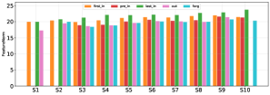
(a)

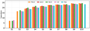
(b)

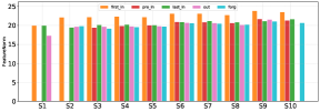
(c)

Figure 26: Features norm of first In set, last In set and the in between In sets along with the features norm of Forg set and Out set for multi-head TinyImageNet Seq. with ResNet

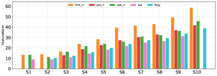
(a)

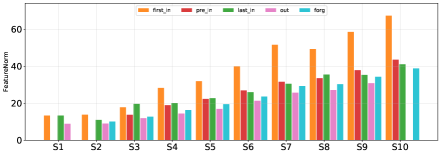
(b)

Figure 27: Features norm of first In set, last In set and the in between In sets along with the features norm of Forg set and Out set for ER  under shared-head on TinyImageNet Seq. with ResNet

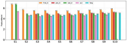
(a)

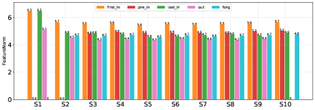
(b)

Figure 28: Features norm of first In set, last In set and the in between In sets along with the features norm of Forg set and Out set for SSIL  under shared-head on TinyImageNet Seq. with ResNet.

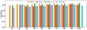
(a)

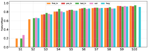
(b)

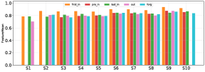
(c)

Figure 29: Features mean of first In set, last In set and the in between In sets along with the features mean of Forg set and Out set for multi-head TinyImageNet Seq. with ResNet.

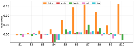
(a)

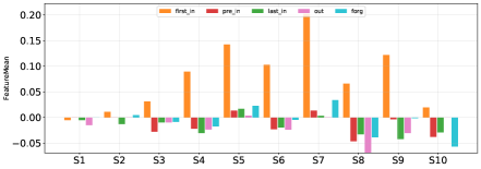
(b)

Figure 30: Features mean of first In set, last In set and the in between In sets along with the features mean of Forg set and Out set for ER  under shared-head on TinyImageNet Seq. with ResNet.

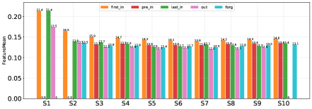
(a)

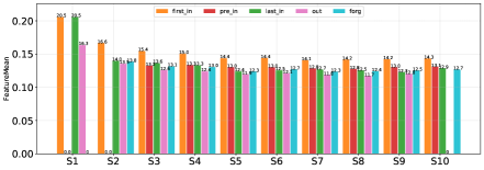
(b)

Figure 31: Features mean of first In set, last In set and the in between In sets along with the features mean of Forg set and Out set for SSIL  under shared-head on TinyImageNet Seq. with ResNet.

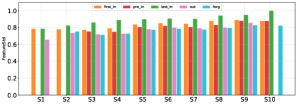
(a)

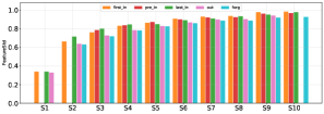
(b)

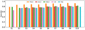
(c)

Figure 32: Features std. of first In set, last In set and the in between In sets along with the features std. of Forg set and Out set for multi-head TinyImageNet Seq. with ResNet.

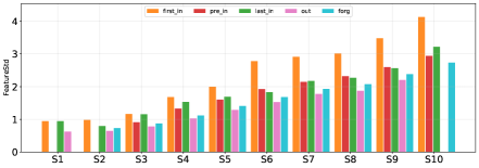
(a)

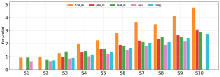
(b)

Figure 33: Features std. of first In set, last In set and the in between In sets along with the features std. of Forg set and Out set for ER  under shared-head on TinyImageNet Seq. with ResNet.

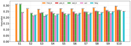
(a)

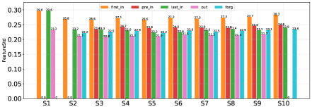
(b)

Figure 34: Features std. of first In set, last In set and the in between In sets along with the features mean of Forg set and Out set for SSIL  under shared-head on TinyImageNet Seq. with ResNet.

References

- Ahn et al. (2021) Hongjoon Ahn, Jihwan Kwak, Subin Lim, Hyeonsu Bang, Hyojun Kim, and Taesup Moon. Ss-il: Separated softmax for incremental learning. In Proceedings of the IEEE/CVF International Conference on Computer Vision, pp. 844–853, 2021.
- Aljundi et al. (2018) Rahaf Aljundi, Francesca Babiloni, Mohamed Elhoseiny, Marcus Rohrbach, and Tinne Tuytelaars. Memory aware synapses: Learning what (not) to forget. In European Conference on Computer Vision, pp. 144–161. Springer, 2018.
- Aljundi et al. (2019a) Rahaf Aljundi, Eugene Belilovsky, Tinne Tuytelaars, Laurent Charlin, Massimo Caccia, Min Lin, and Lucas Page-Caccia. Online continual learning with maximal interfered retrieval. In H. Wallach, H. Larochelle, A. Beygelzimer, F. d'Alché-Buc, E. Fox, and R. Garnett (eds.), Advances in Neural Information Processing Systems, volume 32. Curran Associates, Inc., 2019a. URL https://proceedings.neurips.cc/paper/2019/file/15825aee15eb335cc13f9b559f166ee8-Paper.pdf.
- Aljundi et al. (2019b) Rahaf Aljundi, Klaas Kelchtermans, and Tinne Tuytelaars. Task-free continual learning. In Proceedings of the IEEE Conference on Computer Vision and Pattern Recognition, pp. 11254–11263, 2019b.
- Aljundi et al. (2019c) Rahaf Aljundi, Min Lin, Baptiste Goujaud, and Yoshua Bengio. Online continual learning with no task boundaries. CoRR, abs/1903.08671, 2019c. URL http://arxiv.org/abs/1903.08671.
- An & Cho (2015) Jinwon An and Sungzoon Cho. Variational autoencoder based anomaly detection using reconstruction probability. Special Lecture on IE, 2(1):1–18, 2015.
- Antunes & Biala (2012) M Antunes and Grazyna Biala. The novel object recognition memory: neurobiology, test procedure, and its modifications. Cognitive processing, 13(2):93–110, 2012.
- Bendale & Boult (2015) Abhijit Bendale and Terrance Boult. Towards open world recognition. In Proceedings of the IEEE Conference on Computer Vision and Pattern Recognition, pp. 1893–1902, 2015.
- Bodesheim et al. (2015) Paul Bodesheim, Alexander Freytag, Erik Rodner, and Joachim Denzler. Local novelty detection in multi-class recognition problems. In 2015 IEEE Winter Conference on Applications of Computer Vision, pp. 813–820. IEEE, 2015.
- Boudiaf et al. (2020) Malik Boudiaf, Jérôme Rony, Imtiaz Masud Ziko, Eric Granger, Marco Pedersoli, Pablo Piantanida, and Ismail Ben Ayed. A unifying mutual information view of metric learning: cross-entropy vs. pairwise losses. In European Conference on Computer Vision, pp. 548–564. Springer, 2020.
- Boult et al. (2019) Terrance E Boult, Steve Cruz, Akshay Raj Dhamija, M Gunther, James Henrydoss, and Walter J Scheirer. Learning and the unknown: Surveying steps toward open world recognition. In Proceedings of the AAAI conference on artificial intelligence, volume 33, pp. 9801–9807, 2019.
- Broadbent et al. (2010) Nicola J Broadbent, Stephane Gaskin, Larry R Squire, and Robert E Clark. Object recognition memory and the rodent hippocampus. Learning & memory, 17(1):5–11, 2010.
- de Campos et al. (2009) T. E. de Campos, B. R. Babu, and M. Varma. Character recognition in natural images. In Proceedings of the International Conference on Computer Vision Theory and Applications, Lisbon, Portugal, February 2009.
- Delange et al. (2021) Matthias Delange, Rahaf Aljundi, Marc Masana, Sarah Parisot, Xu Jia, Ales Leonardis, Greg Slabaugh, and Tinne Tuytelaars. A continual learning survey: Defying forgetting in classification tasks. IEEE Transactions on Pattern Analysis and Machine Intelligence, 2021.
- (15) M. Everingham, L. Van Gool, C. K. I. Williams, J. Winn, and A. Zisserman. The PASCAL Visual Object Classes Challenge 2012 (VOC2012) Results. http://www.pascal-network.org/challenges/VOC/voc2012/workshop/index.html.
- Finn et al. (2017) Chelsea Finn, Pieter Abbeel, and Sergey Levine. Model-agnostic meta-learning for fast adaptation of deep networks. In Proceedings of the International Conference on Machine Learning (ICML), 2017.
- Fontanel et al. (2020) Dario Fontanel, Fabio Cermelli, Massimiliano Mancini, Samuel Rota Bulo, Elisa Ricci, and Barbara Caputo. Boosting deep open world recognition by clustering. IEEE Robotics and Automation Letters, 5(4):5985–5992, 2020.
- Hendrycks & Gimpel (2016) Dan Hendrycks and Kevin Gimpel. A baseline for detecting misclassified and out-of-distribution examples in neural networks. arXiv preprint arXiv:1610.02136, 2016.
- Hou et al. (2019) Saihui Hou, Xinyu Pan, Chen Change Loy, Zilei Wang, and Dahua Lin. Learning a unified classifier incrementally via rebalancing. In Proceedings of the IEEE/CVF Conference on Computer Vision and Pattern Recognition, pp. 831–839, 2019.
- Hsu et al. (2020) Yen-Chang Hsu, Yilin Shen, Hongxia Jin, and Zsolt Kira. Generalized odin: Detecting out-of-distribution image without learning from out-of-distribution data. In Proceedings of the IEEE/CVF Conference on Computer Vision and Pattern Recognition, pp. 10951–10960, 2020.
- Joseph et al. (2021) KJ Joseph, Salman Khan, Fahad Shahbaz Khan, and Vineeth N Balasubramanian. Towards open world object detection. In Proceedings of the IEEE/CVF Conference on Computer Vision and Pattern Recognition, pp. 5830–5840, 2021.
- Kirkpatrick et al. (2017) James Kirkpatrick, Razvan Pascanu, Neil Rabinowitz, Joel Veness, Guillaume Desjardins, Andrei A Rusu, Kieran Milan, John Quan, Tiago Ramalho, Agnieszka Grabska-Barwinska, et al. Overcoming catastrophic forgetting in neural networks. Proceedings of the national academy of sciences, pp. 201611835, 2017.
- Krause et al. (2013) Jonathan Krause, Michael Stark, Jia Deng, and Li Fei-Fei. 3d object representations for fine-grained categorization. In Proceedings of the IEEE International Conference on Computer Vision Workshops, pp. 554–561, 2013.
- Lee et al. (2018) Kimin Lee, Kibok Lee, Honglak Lee, and Jinwoo Shin. A simple unified framework for detecting out-of-distribution samples and adversarial attacks. In Advances in Neural Information Processing Systems, pp. 7167–7177, 2018.
- Lee et al. (2017) Sang-Woo Lee, Jin-Hwa Kim, Jaehyun Jun, Jung-Woo Ha, and Byoung-Tak Zhang. Overcoming catastrophic forgetting by incremental moment matching. In Advances in neural information processing systems, pp. 4652–4662, 2017.
- Lee et al. (2020) Soochan Lee, Junsoo Ha, Dongsu Zhang, and Gunhee Kim. A neural dirichlet process mixture model for task-free continual learning. arXiv preprint arXiv:2001.00689, 2020.
- Li & Hoiem (2016) Zhizhong Li and Derek Hoiem. Learning without forgetting. In European Conference on Computer Vision, pp. 614–629. Springer, 2016.
- Liang et al. (2018) Shiyu Liang, Yixuan Li, and R. Srikant. Enhancing the reliability of out-of-distribution image detection in neural networks. In International Conference on Learning Representations, 2018. URL https://openreview.net/forum?id=H1VGkIxRZ.
- Lopez-Paz et al. (2017) David Lopez-Paz et al. Gradient episodic memory for continual learning. In Advances in Neural Information Processing Systems, pp. 6470–6479, 2017.
- Maji et al. (2013) S. Maji, J. Kannala, E. Rahtu, M. Blaschko, and A. Vedaldi. Fine-grained visual classification of aircraft. Technical report, 2013.
- Mancini et al. (2019) Massimiliano Mancini, Hakan Karaoguz, Elisa Ricci, Patric Jensfelt, and Barbara Caputo. Knowledge is never enough: Towards web aided deep open world recognition. In 2019 International Conference on Robotics and Automation (ICRA), pp. 9537–9543. IEEE, 2019.
- Mirzadeh et al. (2020) Seyed Iman Mirzadeh, Mehrdad Farajtabar, Razvan Pascanu, and Hassan Ghasemzadeh. Understanding the role of training regimes in continual learning. arXiv preprint arXiv:2006.06958, 2020.
- Netzer et al. (2011) Yuval Netzer, Tao Wang, Adam Coates, Alessandro Bissacco, Bo Wu, and Andrew Y Ng. Reading digits in natural images with unsupervised feature learning. 2011.
- Nguyen et al. (2017) Cuong V Nguyen, Yingzhen Li, Thang D Bui, and Richard E Turner. Variational continual learning. arXiv preprint arXiv:1710.10628, 2017.
- Nilsback & Zisserman (2008) M-E. Nilsback and A. Zisserman. Automated flower classification over a large number of classes. In Proceedings of the Indian Conference on Computer Vision, Graphics and Image Processing, Dec 2008.
- Qi et al. (2018) Hang Qi, Matthew Brown, and David G Lowe. Low-shot learning with imprinted weights. In Proceedings of the IEEE conference on computer vision and pattern recognition, pp. 5822–5830, 2018.
- Quattoni & Torralba (2009) Ariadna Quattoni and Antonio Torralba. Recognizing indoor scenes. In Computer Vision and Pattern Recognition, 2009. CVPR 2009. IEEE Conference on, pp. 413–420. IEEE, 2009.
- Rebuffi et al. (2017) Sylvestre-Alvise Rebuffi, Alexander Kolesnikov, Georg Sperl, and Christoph H Lampert. icarl: Incremental classifier and representation learning. In Proceedings of the IEEE conference on Computer Vision and Pattern Recognition, pp. 2001–2010, 2017.
- Rolnick et al. (2018) David Rolnick, Arun Ahuja, Jonathan Schwarz, Timothy P. Lillicrap, and Greg Wayne. Experience replay for continual learning. CoRR, abs/1811.11682, 2018. URL http://arxiv.org/abs/1811.11682.
- Schultheiss et al. (2017) Alexander Schultheiss, Christoph Käding, Alexander Freytag, and Joachim Denzler. Finding the unknown: Novelty detection with extreme value signatures of deep neural activations. In German Conference on Pattern Recognition, pp. 226–238. Springer, 2017.
- Simonyan & Zisserman (2014) Karen Simonyan and Andrew Zisserman. Very deep convolutional networks for large-scale image recognition. arXiv preprint arXiv:1409.1556, 2014.
- (42) Stanford. Tiny ImageNet Challenge, CS231N Course. URL https://tiny-imagenet.herokuapp.com/.
- Welinder et al. (2010) P. Welinder, S. Branson, T. Mita, C. Wah, F. Schroff, S. Belongie, and P. Perona. Caltech-UCSD Birds 200. Technical Report CNS-TR-2010-001, California Institute of Technology, 2010.
- Wu et al. (2019) Yue Wu, Yinpeng Chen, Lijuan Wang, Yuancheng Ye, Zicheng Liu, Yandong Guo, and Yun Fu. Large scale incremental learning. In Proceedings of the IEEE/CVF Conference on Computer Vision and Pattern Recognition, pp. 374–382, 2019.
- Yang et al. (2021) Shuo Yang, Peize Sun, Yi Jiang, Xiaobo Xia, Ruiheng Zhang, Zehuan Yuan, Changhu Wang, Ping Luo, and Min Xu. Objects in semantic topology. arXiv preprint arXiv:2110.02687, 2021.
- Zeno et al. (2018) Chen Zeno, Itay Golan, Elad Hoffer, and Daniel Soudry. Task agnostic continual learning using online variational bayes. arXiv preprint arXiv:1803.10123, 2018.
- Zhao et al. (2020) Bowen Zhao, Xi Xiao, Guojun Gan, Bin Zhang, and Shu-Tao Xia. Maintaining discrimination and fairness in class incremental learning. In Proceedings of the IEEE/CVF Conference on Computer Vision and Pattern Recognition, pp. 13208–13217, 2020.