Objective discovery of dominant dynamical processes with intelligible machine learning

Abstract

The advent of big data has vast potential for discovery in natural phenomena ranging from climate science to medicine, but overwhelming complexity stymies insight. Existing theory is often not able to succinctly describe salient phenomena, and progress has largely relied on ad hoc definitions of dynamical regimes to guide and focus exploration. We present a formal definition in which the identification of dynamical regimes is formulated as an optimization problem, and we propose an intelligible objective function. Furthermore, we propose an unsupervised learning framework which eliminates the need for a priori knowledge and ad hoc definitions; instead, the user need only choose appropriate clustering and dimensionality reduction algorithms, and this choice can be guided using our proposed objective function. We illustrate its applicability with example problems drawn from ocean dynamics, tumor angiogenesis, and turbulent boundary layers. Our method is a step towards unbiased data exploration that allows serendipitous discovery within dynamical systems, with the potential to propel the physical sciences forward.

1 Introduction

A salient class of problems in the natural sciences is nonlinear continuum dynamics problems, specifically those pertaining to dynamical systems with uncomputably large numbers of degrees of freedom. Examples span most fields of science; to highlight this diversity we can mention nonlinear waves, plasma dynamics, earthquake dynamics, general relativity, quantum field theory, biochemical reaction-diffusion dynamics, fibrillation dynamics, epilepsy, and turbulent flows (Strogatz, [2018]), as well as fiber optics, droplet formation, wrinkling, biofilm dynamics (Callaham et al., [2021]), weather (Vallis, [2017]), and climate dynamics (Peixoto and Oort, [1992]). The extreme sensitivity of such systems to infinitesimal perturbations (Poincaré, [1905]), known to popular culture as the butterfly effect (Smagorinsky, [1969]), generally prohibits the direct deterministic computation of solutions to governing equations because extreme amounts of high-quality data collection and/or computing power are required to marginally increase limits of predictability.

In lieu of direct computation, scientists and engineers have developed a number of alternatives. A popular method involves the prediction of properties of the probability distributions of the relevant variables. The simplest form of this strategy is to predict the ensemble, spatial, and/or temporal mean of relevant variables. The dynamics of mean variables are sometimes approximately reducible, meaning that local causality can be approximately described by a dominant balance of selected terms from the governing equation (e.g. Callaham et al., [2021]). These local dominant balances, and the boundaries of the solution space in which they are a justifiable truncation of the full dynamics, define what we often refer to as dynamical regimes. In most practical applications the dominant balance of a given dynamical regime is non-asymptotic, meaning that there is no parameter that permits a formal expansion of the equation terms which guarantees the truncation error vanishes according to the limits of said parameter. Much scientific progress has been made by identifying non-asymptotic dominant balances in the aforementioned fields. For example, in a seminal paper on the theory of mid-latitude ocean circulation, Munk, [1950] neglected nonlinear governing equation terms to identify two asymptotic dominant balances within the remaining governing equation terms (Figure 1), which means that this model is non-asymptotic in the context of the full governing equation. Indeed, Sonnewald et al., [2019] identified the same interior dominant balance as Munk, [1950] by using a non-asymptotic unsupervised learning method.

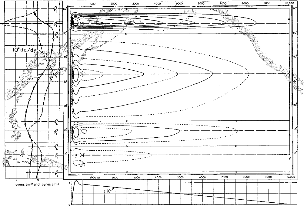
Figure 1: A plot from Munk, [1950] showing the theoretical Pacific Ocean circulation superimposed over the actual coastlines. The interior flow is a dominant balance, referred to as Sverdrup balance, which is adjacent to a western boundary current dominant balance. This idealized circulation correctly hypothesized the dominant mesoscale upper ocean dynamics at mid-latitudes.

Two key attributes of the concept of a dynamical regime are that a) it is local and only applicable to a certain region of sample space, and b) the dominant equation terms are dominant relative to the amplitude of the negligible terms in the same region of sample space. The first attribute defines a partitioning problem: where does one draw the boundary between one regime and another, particularly for non-asymptotic continuum dynamics in which equation term amplitudes may vary smoothly? The second attribute reveals why simple amplitude thresholds cannot be globally applied to a data set that may exhibit two or more dynamical regimes. Instead, the two attributes are closely related and the partitioning of the sample space affects the subset of dominant terms in it, and vice versa. Perhaps the most famous example of this pitfall is the zero drag paradox of d’Alembert, [1752], a false conclusion that was inferred as a consequence of a global threshold that deemed frictional terms negligible everywhere in fluid flow over a sphere. The paradox wasn’t resolved until Prandtl, [1904] discovered friction-induced dynamical regimes within a thin boundary layer over the sphere’s surface, thus enabling the development of boundary layer theory and, subsequently, modern aircraft design, among other applications. We propose that the dynamical regime identification problem can be stated as the question:

what is the optimal partitioning of the data, such that the dominant terms within each partition dominate the negligible terms by the largest amplitude?

Until now, the dynamical regime identification problem has not been formulated as a mathematical expression. In this Article, we 1) mathematically formalize the dynamical regimes problem as an optimization problem, 2) propose an objective function to quantify the optimal solution to this problem, 3) propose a custom dimensionality reduction algorithm for the dynamical regime problem, and 4) propose an unsupervised learning framework (Kohavi and John, [1997], Dy and Brodley, [2004]) for solving the problem, drawing upon recent successes of unsupervised learning as a tool for partitioning dynamical regimes (Sonnewald et al., [2019], Callaham et al., [2021]) and upon the success of dimensionality reduction algorithms (Van Der Maaten et al., [2009]) for labeling dominant balances (Callaham et al., [2021]). Crucially, the proposed objective function defines the optimal for a given clustering algorithm, and it permits objective comparison of the results of different choices of algorithms. By defining the optimal for the dynamical regime problem, we enable the discovery of dominant balances without any prerequisite domain knowledge: the user need not know what dynamical regimes exist in the data before applying our framework.

Throughout this article, we will refer to the dimensionality reduction algorithms as hypothesis selection to emphasize that our unsupervised learning framework is analogous to the scientific method: it proposes dominant balance hypotheses and subsequently tests the fit of those hypotheses to the data. This choice of words reflects our perspective that machine learning for scientific applications should be developed towards the goal of creating an artificial scientific collaborator by systematizing the scientific method, rather than continuing the current paradigm in which the logic of highly predictive algorithms is extremely difficult to discern (Rudin, [2019]). Furthermore, this choice of words also reflects that our formal mathematical definition of the problem of dynamical regime identification is intentionally constructed so that it can be tackled by physical, mathematical, or AI scientists.

2 Methods

In this section we propose a formal mathematical definition of the dynamical regimes problem, an objective function that defines optimal solutions to the dynamical regimes problem, and an unsupervised learning framework that solves the dynamical regimes problem.

2.1 Problem formulation

Given the array of data $\mathbf{E}=[\mathbf{e}_{1},...,\mathbf{e}_{N}]$, consisting of $N$ observations of the $D-$dimensioned vector of equation terms $\mathbf{e}_{n}$, we seek to label each observation with a $D-$dimensioned hypothesis vector $\mathbf{h}_{n}$, where $h_{ni}\in\{0,1\}$ for each $n^{th}$ observation of the $i^{th}$ equation term. We assume that the equation is closed, $\sum_{i=1}^{D}e_{ni}=0$, for all observations. The entire array of data is labeled by $\mathbf{H}=[\mathbf{h}_{1},...,\mathbf{h}_{N}]$, and the zeros of each hypothesis vector $\mathbf{h}_{n}$ indicate the equation terms in $\mathbf{e}_{n}$ that are neglected. We choose a global objective function $\mathcal{M}(\mathbf{E},\mathbf{H})$, such that the optimal fit of hypotheses for the entire data array, $\mathbf{H}_{\text{opt}}$, can be obtained by varying the hypotheses $\mathbf{H}$ to find $\max\mathcal{M}(\mathbf{E},\mathbf{H})$,

$$\mathbf{H}_{\text{opt}}=\begin{cases}\operatorname*{argmax}\limits_{\mathbf{H}}\mathcal{M}(\mathbf{E},\mathbf{H})\quad:\quad\max\mathcal{M}(\mathbf{E},\mathbf{H})>\mathcal{M}(\mathbf{E},\mathbf{1})\\ \mathbf{1}\hskip 82.51299pt\quad:\quad\max\mathcal{M}(\mathbf{E},\mathbf{H})\leq\mathcal{M}(\mathbf{E},\mathbf{1})\end{cases},$$ (1)

where $\mathbf{H}=\mathbf{1}$ is an array of ones indicating all equation terms are retained for the entire data array. We use the notation convention of Bishop, [2006] in which scalars are presented in italics, lower case bold variables represent one dimensional arrays, and upper case bold variables represent two or higher dimensional arrays.

We propose Equation 1 as the definition of the dynamical regime problem, in which one seeks to partition the observations $\mathbf{E}$ into different regimes with different dominant balances, as labeled by $\mathbf{H}_{\text{opt}}$. The dominant balances within $\mathbf{H}_{\text{opt}}$ can be assigned by traditional, heuristic methods for eliminating equation terms, such as using characteristic scales to estimate term magnitudes (Tennekes et al., [1972]), or they can be assigned by partitioning the data using clustering algorithms and subsequently labeling all observations in each cluster with the same dominant balance by using dimensionality reduction algorithms (Callaham et al., [2021]). Next, we propose a simple, intelligible objective function for $\mathcal{M}(\mathbf{E},\mathbf{H})$, and demonstrate how it can be deployed to find $\mathbf{H}_{\text{opt}}$ in Equation 1.

2.2 An intelligible objective function

The global objective function $\mathcal{M}(\mathbf{E},\mathbf{H})$ in Equation 1 must favor the selection of dominant equation terms intelligibly, where we define intelligible as both interpretable (Rudin, [2019]) and congruent with domain knowledge (Wang et al., [2018]). We construct the objective function such that the definition of the optimal satisfies two conditions for each regime:

1. the magnitude difference between the selected dominant terms and the negligible terms must be maximized;

2. the magnitude difference between the terms within the selected dominant set must be minimized;

and such that the global optimal for possibly many regimes satisfies criteria 1) and 2) for the largest weighted percentage of samples. If the first condition is not satisfied, then all equation terms should be retained, i.e., they are all equally dominant.

We begin by defining the local order-of-magnitude score, $\mathcal{M}_{n}(\mathbf{e}_{n},\mathbf{h}_{n})$, hereafter the local magnitude score, pertaining to a single observation, which measures the magnitude gap between dominant terms $\mathbf{h}_{n}\cdot\mathbf{e}_{n}$ and negligible terms $|\mathbf{h}_{n}-\mathbf{1}|\cdot\mathbf{e}_{n}$ in a single observation $\mathbf{e}_{n}$ (recall that the terms that are selected as dominant are labeled by ${h}_{ni}=1$, and the neglected terms are labeled by ${h}_{ni}=0$). Define $\mathrm{F}=\{1,...,D\}$ as the index set (Munkres, [2000]) of the indices of the full set equation terms in vector $\mathbf{e}_{n}$, such that

$$\mathbf{e}_{n}=\bigcup_{i\in\mathrm{F}}e_{ni},$$ (2)

for observation $n$ such that $1\leq n\leq N$.

We refer to the binary sets that represent the dominant terms as hypotheses, because they represent informal equation truncations that are not guaranteed to have asymptotic properties. The hypotheses for the entire data set $\mathbf{E}$ form an array, $\mathbf{H}$, which has the same dimensions as $\mathbf{E}$, namely number of samples $\times$ number of equation terms. The hypothesis vectors for each observation can be expressed as

$$\mathbf{h}_{n}=\bigcup_{i\in\mathrm{F}}h_{ni},$$ (3)

where $\mathbf{h}_{n}$ is an indicator function (Cormen et al., [2009]) that consists entirely of ones and zeros, which represent selected dominant terms and negligible terms, respectively.

The indices of elements in $\mathbf{e}_{n}$ that are selected as dominant terms by the hypothesis $\mathbf{h}_{n}$ form the selection index set $\mathrm{S}_{n}$, where

$$\mathrm{S}_{n}\subseteq\mathrm{F}.$$ (4)

Note that the number of selected elements may vary for each observation $n$, and if $\mathrm{S}_{n}=\mathrm{F}$ then $\mathbf{h}_{n}=\mathbf{1}$ and no equation terms are neglected. It follows that the remainder index set $\mathrm{R}_{n}$ for the $n^{th}$ observation is defined by set subtraction,

$$\mathrm{R}_{n}=\mathrm{F}-\mathrm{S}_{n},$$ (5)

and, therefore, the remainder index set and selected index set are non-overlapping,

$$\mathrm{R}_{n}\cap\mathrm{S}_{n}=\varnothing.$$ (6)

Thus the cardinality, or size, of the selected index set and remainder index set are $2\leq\text{card}(\mathrm{S}_{n})\leq D$ and $0\leq\text{card}(\mathrm{R}_{n})\leq D-2$, respectively. The lower bound of two selected terms is not necessary nor required; we impose it because a dominant balance of just one term is conceptually ambiguous. Let the arrays of selected and remainder equation terms from $\mathbf{e}_{n}$ be $\mathbf{s}_{n}$ and $\mathbf{r}_{n}$, respectively. $\mathbf{s}_{n}$ and $\mathbf{r}_{n}$ are normalized by the smallest element of $\mathbf{e}_{n}$ and defined as

$$\mathbf{s}_{n} =\frac{\bigcup_{i\in\mathrm{S}_{n}}|{e}_{ni}|}{\min\big{(}\bigcup_{i\in\mathrm{F}}|{e}_{ni}|\big{)}},$$ (7)

$$\mathbf{r}_{n} =\frac{\bigcup_{i\in\mathrm{R}_{n}}|{e}_{ni}|}{\min\big{(}\bigcup_{i\in\mathrm{F}}|{e}_{ni}|\big{)}},$$ (8)

respectively. If $\min(\bigcup_{i\in\mathrm{F}}|{e}_{ni}|)=0$, then the minimum non-zero absolute valued element of $\mathbf{e}_{n}$ replaces the denominators in Equations 7 and 8. Let the relative magnitude gap between the normalized subsets, $\Gamma$, be defined as a scalar for each $n^{th}$ observation:

$$\Gamma_{n}=\begin{cases}\frac{\log_{10}(\min(\mathbf{s}_{n})-\max(\mathbf{r}_{n}))}{\log_{10}(\min(\mathbf{s}_{n})+\max(\mathbf{r}_{n}))}\quad\text{if}\quad\min(\mathbf{s}_{n})>\max(\mathbf{r}_{n})\\ 0\hskip 101.00728pt\text{if}\quad\min(\mathbf{s}_{n})\leq\max(\mathbf{r}_{n})\end{cases}.$$ (9)

The magnitude gap $\Gamma$ is normalized such that $\Gamma\in[-\infty,1]$, and the floor condition if $\Gamma<0$ then set $\Gamma=0$ is implemented to correct for spurious large amplitude negative values of $\Gamma$ that arise as $\min(\mathbf{s}_{n})\rightarrow\max(\mathbf{r}_{n})$ from above. $\Gamma\rightarrow 1$ as the number of orders of magnitude between the element with the minimum absolute value of the selected subset and element with the maximum absolute value of the remainder subset approaches infinity, and if $\Gamma=1$ then the hypothesis that the terms in the selected subset dominate the terms in the remainder subset is exact (for any numerical implementation the optimal is limited by machine precision, so $\Gamma\approx 1$). If the magnitude difference between the two subsets vanishes, then $\Gamma\rightarrow 0$, and if a remainder subset term exceeds the absolute magnitude of the selected subset, then the hypothesis does not represent a dominant balance, and $\Gamma=0$ is prescribed.

Since the goal is to choose the selected subset, $\mathbf{s}_{n}$, such that it corresponds to the dominant terms, the feature magnitudes of the selected subset should be approximately the same. Otherwise, the smallest magnitude term(s) in the selected subset should be removed from that subset and added to the remainder subset. To penalize large absolute magnitude differences within the selected subset, we introduce the scalar penalty for the $n^{th}$ observation,

$$\Omega_{n}=\log_{10}(\max(\mathbf{s}_{n}))-\log_{10}(\min(\mathbf{s}_{n}))\in[0,\infty).$$ (10)

A base 10 logarithm is chosen for the penalty because it corresponds most directly to the notion of orders of magnitude. If $\Omega_{n}\rightarrow 0$, the absolute magnitudes of the selected subset terms approach uniformity.

We define the local magnitude score for the $n^{th}$ observation $\mathcal{M}_{n}(\mathbf{e}_{n},\mathbf{h}_{n})$ as

$$\mathcal{M}_{n}(\mathbf{e}_{n},\mathbf{h}_{n})=\frac{\Gamma_{n}}{1+\Omega_{n}}\in[0,1].$$ (11)

By construction, the local magnitude score is a) invariant to the magnitude of the feature vector $\mathbf{x}_{n}$ and b) invariant to the sign of the elements of the feature vector,

$$\mathcal{M}_{n}(\mathbf{e}_{n},\mathbf{h}_{n})=\mathcal{M}_{n}(\pm c\mathbf{e}_{n},\mathbf{h}_{n}),$$ (12)

where $c$ is a positive scalar constant. Therefore, the score is invariant to the choice of dimensional or non-dimensional equations, and, equivalently, it can be applied to Buckingham $\Pi$ theorem to identify dominant $\Pi$ groups. Readers unfamiliar with the Buckingham $\Pi$ theorem and how it pertains to the non-dimensionalization of partial differential equations are referred to Zohuri, [2017].

Finally, we propose the global magnitude score $\mathcal{M}(\mathbf{X},\mathbf{H})$ as an objective function that satisfies Equation 1, which yields a single score for the fit of the hypotheses for all $N$ observations, $\mathbf{H}$, to the entire data set $\mathbf{E}$,

$$\mathcal{M}(\mathbf{E},\mathbf{H})=\frac{\sum_{n=1}^{N}{w}_{n}\cdot\mathcal{M}_{n}(\mathbf{e}_{n},\mathbf{h}_{n})}{\sum_{n=1}^{N}{w}_{n}},$$ (13)

where the array of weights $\mathbf{w}=[w_{1},...,w_{N}]$ are the discrete differentials of the observed domain, e.g. space and/or time differentials. For example, if the $N$ observations of data set $\mathbf{E}$ are of equation terms distributed across a two-dimensional space, then the global magnitude score in Equation 13 is the area-weighted average of all of the scores for each observation. The full set score for the entire data set can be expressed as $\mathcal{M}(\mathbf{E},\mathbf{1})$, where $\mathbf{1}=\{\mathbf{1}_{1},...,\mathbf{1}_{N}\}$. Equation 13 is an evaluation of the fit of potentially many different hypotheses to potentially many different regimes within data set $\mathbf{E}$.

2.2.1 Combinatorial hypothesis selection

We propose a simple hypothesis selection algorithm that we will refer to as the combinatorial hypothesis selection (CHS) algorithm. Since the number of all possible hypotheses for an equation is a permutation of two types (0 or 1) with repetition allowed, the number of possible hypotheses is $\mathcal{O}(2^{D})$. If the number of equation terms, $D$, is not large, then hypotheses can be feasibly generated by calculating the magnitude score (Equation 11) for all possible hypotheses and then selecting the hypothesis that is awarded the highest score. Equation 11 can be applied to a single data sample or to an average of samples. The exponential time complexity limits the feasibility of computing CHS to equations with relatively few terms.

2.3 Unsupervised learning framework

In unsupervised learning, the goal is to partition the data into labeled groups, or clusters, that reveal underlying patterns of sparsity in the data. Clustering algorithms are a class of unsupervised machine learning algorithms that yield a finite set of categories to describe a given data set according to similarities or relationships among its objects (MacQueen et al., [1967], Hartigan, [1975]). Clustering performance scores are objective measures that define the optimal partitioning of the data by quantitatively evaluating the consistency of the statistical properties of the clusters with hypothesized statistical properties of the data. For example, if one wishes to find convex Euclidean (hyper-spherical or hyper-elliptical) clusters, then the silhouette score (Rousseeuw, [1987]) is a useful measure of the fit of the clustering algorithm labels to convex groups of features that may present in the data. Clustering performance scores are particularly useful because clustering results are sensitive to the choice of algorithm parameters (Pedregosa et al., [2011]) and there is no definition of a cluster that is universal to all clustering algorithms (Estivill-Castro, [2002]).

The objective score $\mathcal{M}(\mathbf{E},\mathbf{H})$ in Equation 13 is a quantitative measure of the sparsity of equation terms and a criterion for a framework that includes both clustering and hypothesis selection algorithms. Given equation data set $\mathbf{E}$, clustering algorithms can be coupled with hypothesis selection methods to solve the dynamical regime problem by labeling regions of $\mathbf{E}$ with dominant balance hypotheses $\mathbf{H}$ (Callaham et al., [2021]). We propose a framework for unsupervised learning (Kohavi and John, [1997], Dy and Brodley, [2004]) that utilizes the objective criterion $\mathcal{M}(\mathbf{E},\mathbf{H})$ to loop over algorithm parameters to find optimal dominant balance hypotheses, $\mathbf{H}_{\text{opt}}$, as defined by Equation 1. The framework, akin to the scientific method, is depicted in Figure 2, in which the dynamical regime problem is broken into partitioning, hypothesis selection, and hypothesis testing tasks. The left column describes the historical heuristic method for solving the dynamical regime problem and the right column depicts our algorithmic framework.

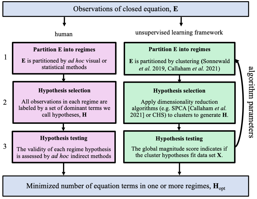
Figure 2: Diagram of the dynamical regime problem, with partitioning and empirical scaling analysis performed by a human (left column), and algorithms capable of performing said tasks (right column). The loop over algorithm parameters illustrates the procedure for obtaining $\mathbf{H}_{\text{opt}}$ in Equation 1.

2.3.1 Partitioning dynamical regimes

The first task shown in Figure 2, row 1, is to classify different dynamical regimes within the feature data (equation terms) with a clustering algorithm. For humans, this task is a simple pattern recognition task of merely noticing markedly different dynamics in one spatio-temporal region versus another: the act of observing and discerning distinct dynamical regimes. Sonnewald et al., [2019] suggested that if the governing equations of the observed dynamics are known, then the heuristic act of noticing different dynamical regimes can be formulated as a partitioning task that can be performed by a clustering algorithm. Dynamical regimes are conventionally defined by dominant average balances, where the averaging is applied to the sample space (e.g. space and/or time). Parametric clustering algorithms like Expectation-Maximization (EM, Bishop, [2006]) clustering algorithms, which assume that the data are drawn from known parametric families of distributions (e.g. Gaussian), are consistent with this precedent, but the cluster means and variances suffer from a sensitivity to outliers (Campello et al., [2015]). Outliers can distort the parametric model density functions by masking or swamping them to produce erroneous model means and to erroneously enlarged or reduced model variances (Pearson and Sekar, [1936]). While nonparametric clustering algorithms detect and remove outliers (Hartigan, [1975], Campello et al., [2015]), the optimal choice of clustering algorithm for the dynamical regime problem is not obvious and will depend on the properties of both the dynamical information and the noise in each data set. The equation data should be standardized in accordance with the choice of clustering algorithm. Crucially, the objective criterion $\mathcal{M}(\mathbf{E},\mathbf{H})$ defines the optimal for a given clustering algorithm, and it permits objective comparisons between the optimal results of different clustering algorithms.

2.3.2 Hypothesis selection

The second task shown in Figure 2 is to generate hypotheses $\mathbf{H}$ for all samples. Humans typically perform this task by carefully estimating characteristic scales from observations, subsequently estimating the magnitude of non-dimensional parameters, and finally choosing which equation terms are negligible in each regime (Zohuri, [2017]). The goal of hypothesis selection is to assign the same hypotheses to all samples within a regime. This is achieved by applying statistical dimensionality reduction techniques to assign active or inactive (negligible) labels to the equation terms uniformly for all samples within each cluster. Therefore, hypothesis selection algorithms are merely algorithms selected from the subclass of dimensionality reduction techniques that pertain to convex data (Van Der Maaten et al., [2009]). This was first demonstrated in the context of equation-spaces by Callaham et al., [2021], who proposed sparse principal component analysis (SPCA, Zou et al., [2006]) as a tenable hypothesis selection algorithm because it labels features with small variances as negligible by performing a least absolute shrinkage and selection operator (LASSO, Tibshirani, [1996]) regression on the principal axes from principal component analysis. SPCA is therefore notionally consistent with EM clustering algorithms (e.g. $K-$means, Gaussian Mixture Models) in the sense that both clustering algorithm and hypothesis selection algorithm are parametric and specifically assume that the sampled cluster feature variances are representative of a unimodal Gaussian or near-Gaussian cluster feature distributions.

2.3.3 Hypotheses testing

The final task shown in Figure 2 is to evaluate the fit of the hypotheses to each regime. In the past, this task has been performed both directly and indirectly. If the observations included not only enough data to estimate the characteristic scales but also enough data to estimate the amplitudes of the equation terms, then direct evaluations of which equation terms are negligible could be performed. Otherwise, hypotheses were indirectly validated through the validation of predictive models that neglected the same equation terms (e.g. aerodynamic drag forces predicted by the “law of the wall”). However, in the case of direct validation, an arbitrary threshold that separates dominant from negligible terms must be selected. The threshold must be applied locally and not globally, meaning it must be applied to each regime individually, because the absolute equation term magnitudes can vary from regime to regime, as exemplified by d’Alembert’s paradox (see Introduction, also Currie, [2016]). Therefore, by defining the optimal hypotheses for the dynamical regime problem, Equation 1 formalizes direct validation of hypotheses. The framework loop over clustering and hypothesis selection algorithm parameters depicted in Figure 2 is thus conceptually akin to a human applying different characteristic scales and/or methods of estimating characteristic scales while searching for the optimal hypotheses for a given data set.

3 Examples

In this section we demonstrate the use of the local magnitude score and the unsupervised learning framework to solve the problem of identification of dynamical regimes, using examples drawn from a variety of disciplines. Complete discussions of the dynamics of each example are beyond the scope of this Article and interested readers are referred to the corresponding citations.

3.1 Local magnitude score example

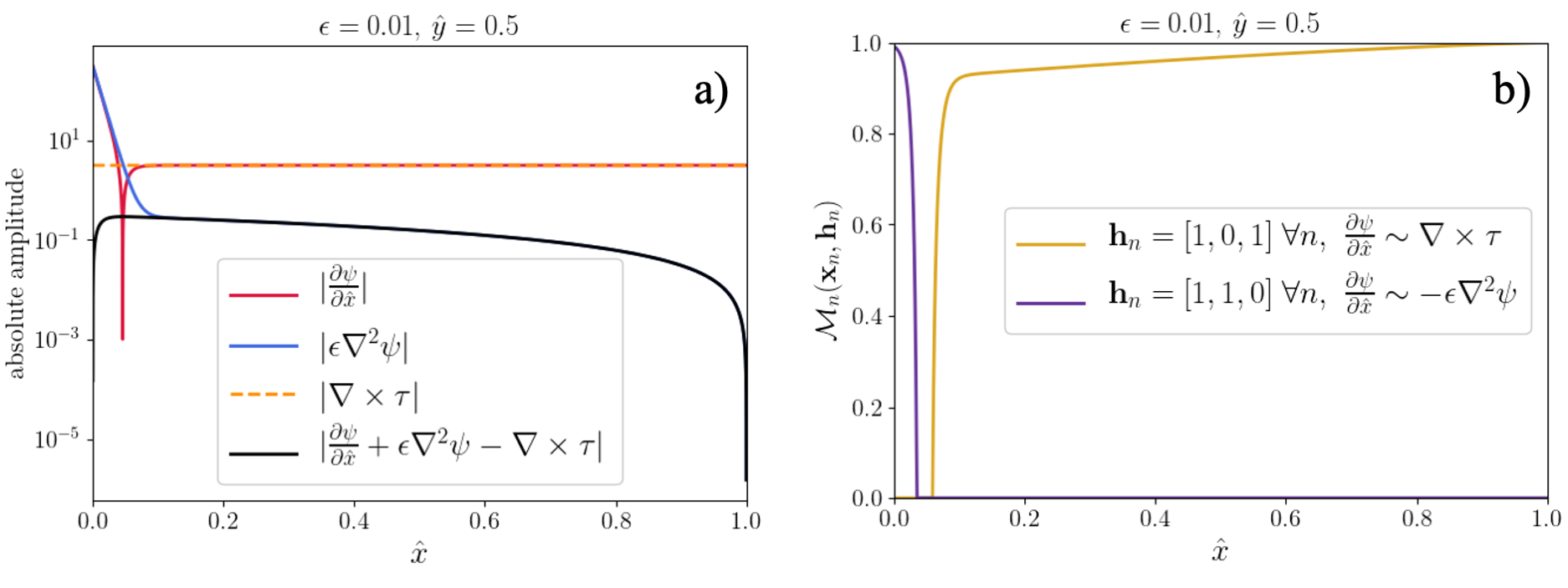
Figure 3: The local magnitude score applied to Munk’s asymptotic matching problem for wind-driven ocean circulation, using the low-order diffusion model of Vallis, [2017]. Panel $a)$ shows the magnitude of each equation term as a function of $\hat{x}$ if $\hat{y}=0.5$, and panel $b)$ shows the local magnitude for two hypotheses, the purple line corresponding to a western boundary current balance and the yellow line corresponding to Sverdrup balance.

Consider the asymptotic matching problem presented by Munk, [1950] in his analysis of the dynamics of wind-driven oceanic heat transport (Figure 1). The two-dimensional steady-state circulation is described by its non-dimensional streamfunction $\psi(\hat{x},\hat{y})$, forced by the non-dimensional wind stress $\boldsymbol{\tau}=-\cos(\pi\hat{y})\mathbf{i}$, and governed by the equation

$$\overbrace{\frac{\partial\psi}{\partial\hat{x}}}^{\begin{subarray}{c}\text{advection of}\\ \text{ planetary vorticity}\end{subarray}}+\hskip 8.53581pt\overbrace{\epsilon\nabla^{2}\psi}^{\begin{subarray}{c}\text{diffusive}\\ \text{torque}\end{subarray}}\hskip 5.69054pt=\hskip 5.69054pt\overbrace{\nabla\times\boldsymbol{\tau}}^{\begin{subarray}{c}\text{wind}\\ \text{stress curl}\end{subarray}},$$ (14)

where $0<\epsilon\ll 1$, $\nabla^{2}=\partial^{2}/\partial\hat{x}^{2}+\partial^{2}/\partial\hat{y}^{2}$, $\hat{x}$ and $\hat{y}$ are the longitudinal and latitudinal coordinates, respectively, the ocean basin geometry is idealized as a square, $0\leq\hat{x}\leq 1$, $0\leq\hat{y}\leq 1$, and we employ the lower-order diffusive torque model of Vallis, [2017] for illustrative purposes. The method of matched asymptotic expansions can be applied to obtain the solution (Vallis, [2017])

$$\psi(\hat{x},\hat{y})\approx(1-x-\mathrm{e}^{-\hat{x}/\epsilon})\pi\sin(\pi\hat{y}),$$ (15)

which approximately satisfies impermeable flow boundary conditions ($\psi=0$) on both the east and west sides of the ocean basin. The solution to this problem, and therefore each possible dynamical regime or truncation of Equation 14, are referred to as asymptotic because the conservation properties converge consistently with $\mathcal{O}(\epsilon)$. However, Equation 14 is an idealized and truncated form of the barotropic vorticity equation, and therefore Equation 15 is not an asymptotic solution of the full vorticity equation.

Figure 3a) shows the magnitude of each equation term in the asymptotic matching problem for $\epsilon=0.01$ at $\hat{y}=0.5$, such that each $n^{th}$ observation $\mathbf{e}_{n}=[\frac{\partial\psi}{\partial\hat{x}},\epsilon\nabla^{2}\psi,\nabla\times\boldsymbol{\tau}]_{n}$ corresponds to a discrete location in the $x$ direction. Figure 3b) shows the variation of local magnitude score over $\hat{x}$ at $\hat{y}=0.5$ for two dominant balances: a dominant balance between planetary advection and diffusion (a.k.a. western boundary current, $\mathbf{h}_{n}=[1,0,1]$, purple) and a dominant balance between the planetary advection and the wind stress curl (a.k.a. Sverdrup balance, $\mathbf{h}_{n}=[1,1,0]$, yellow).

Figure 3b) indicates that, at $\hat{y}=0.5$, the western boundary current and Sverdrup dynamical regimes are unambiguously dominant over distinct ranges of $\hat{x}$ separated by a gap at $\hat{x}\approx 0.04$. However, the boundaries between different dynamical regimes are often not as obvious as in Figure 3b) and an objective method for partitioning the regimes is required. In the next section, we demonstrate how observations can be partitioned into distinct regimes by using the unsupervised learning methods of Sonnewald et al., [2019] and Callaham et al., [2021], which can then be evaluated using the objective function defined by Equation 1 to find the optimal partitioning and labeling of each dynamical regime.

3.2 Unsupervised learning framework examples

3.2.1 Synthetic data

A simple framework test case is a two-dimensional array of data with an even number of features where half of the features are many orders of magnitude larger in one half of the domain and vice versa. Multiplicative sinusoidal noise is added to give the two regions variance that is proportional to 10% of the signal amplitude in each region. The two regions can be considered dynamical regimes: in each, half of the terms dominate the other equation terms by two orders of magnitude. The regions of dominant terms are prescribed by a perturbed Heaviside step function $\mathcal{H}$, such that:

$$\mathbf{e}_{i}(\hat{x},\hat{y}) =(-1)^{i}{\eta}(\hat{y})(\lambda\mathcal{H}(\phi)+\beta),$$ (16)

$$\eta(\hat{y}) =\eta_{0}\sin(\omega\hat{y}),$$ (17)

$$\phi =\begin{cases}\hat{y}-0.5\quad\forall i<D/2\\ 0.5-\hat{y}\quad\forall i\geq D/2\end{cases},$$ (18)

where $\hat{x}$ and $\hat{y}$ are spatial coordinates. The equation closes exactly for all $n$ samples, $\sum_{i=1}^{D}e_{ni}=0$, and the prescribed coefficients are shown in Table 1.

$\lambda$	$\beta$	$\eta_{0}$	$\omega$
$10^{1}$	$10^{-1}$	$10^{-1}$	$10\pi$

Table 1: Prescribed coefficients for the synthetic data set

Figure 4a) shows the synthetic data $e_{ni}$ consisting of $D=8$ equation terms and featuring two regimes in which the dominant terms have amplitudes of $\mathcal{O}(10)$. Each regime is composed of four equation terms, and the inactive terms have amplitudes of $\mathcal{O}(10^{-1})$, and the regimes are separated by a discontinuity at $\hat{y}=0.5$ as prescribed by Equation 16.

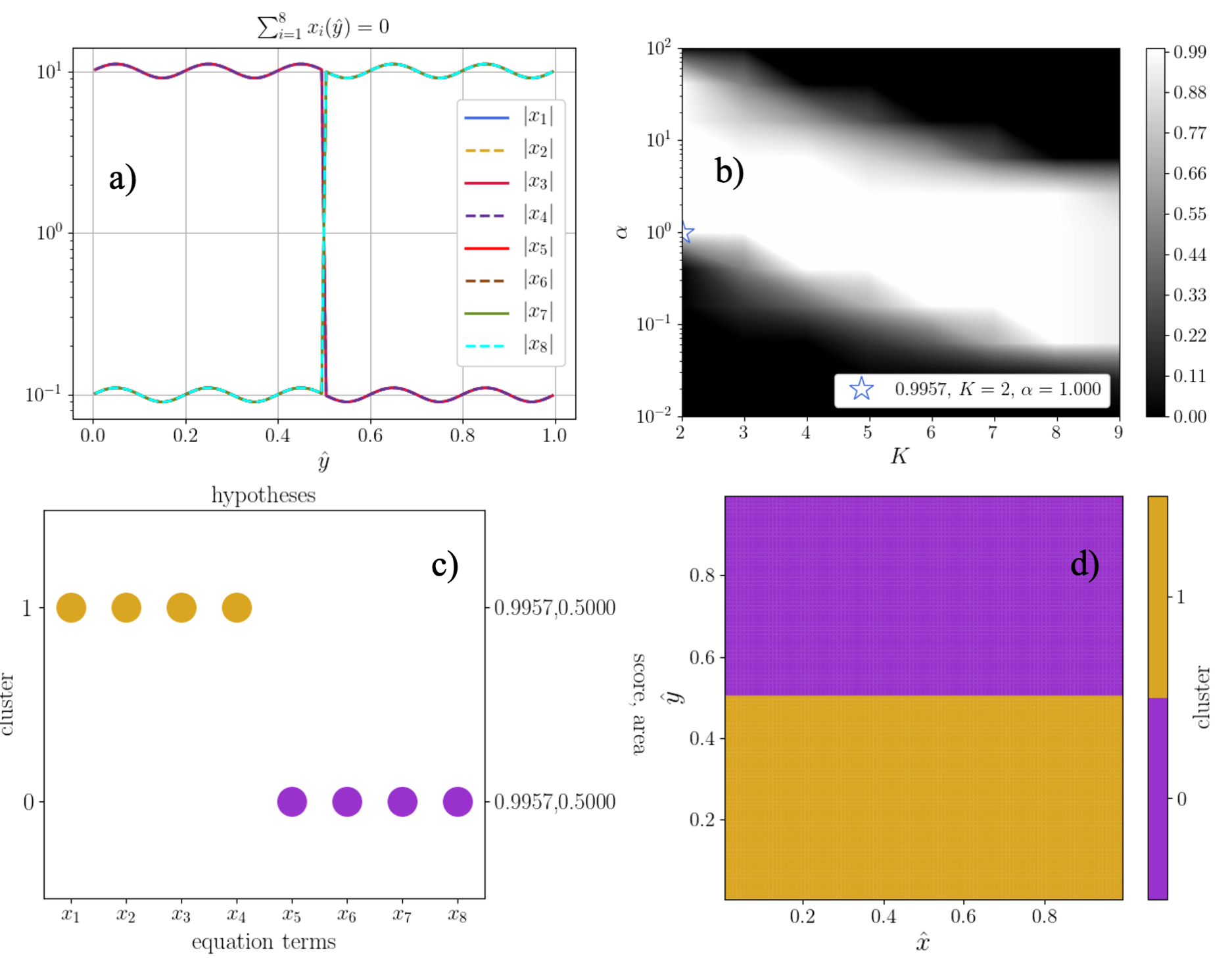
Figure 4: The synthetic data for all $\hat{y}$ at constant $\hat{x}$ is shown in panel $a)$. Panel $b)$ shows the variation global magnitude score as the number of prescribed clusters for $K-$means and the LASSO regression coefficient $\alpha$ for SPCA are varied. Panels $c)$ and $d)$ show the dominant balances and their spatial distribution for the optimal results that occur in the white band in $b)$ which correspond to a global magnitude score of 0.996.

Figures 4b), 4c), and 4d) show the unsupervised learning framework results for the synthetic data using $K-$means for clustering and SPCA for hypothesis selection. Figure 4b) shows the variation of the global magnitude score $\mathcal{M}(\mathbf{E},\mathbf{H})$ as $\alpha$, the LASSO regression coefficient for SPCA, and $K$, the prescribed number of clusters for $K-$means clustering, are varied. The optimal result is marked with the blue star. Figure 4c) shows the dominant equation terms of the optimal result and Figure 4d) shows the spatial distribution of the two clusters of the optimal result. The clusters and their distributions for all of the $\alpha$ and $K$ values within the white band where the global magnitude score is $\mathcal{M}(\mathbf{E},\mathbf{H})=0.9957$ in Figure 4b) are identical to those shown in Figures 4c) and 4d).

The same optimal results as shown in Figures 4b), 4c), and 4d) were obtained by using $K-$means clustering and CHS, by using Hierarchical Density-Based Scan (HDBSCAN) and SPCA, as well as by using HDBSCAN and the CHS algorithm. The robustness of the results shown in Figures 4b), 4c), and 4d) arises because the magnitude separation and spatial distributions of the dominant balances that are implicit in the synthetic data (see Figure 4a)) are pronounced in both amplitude and the sharpness of the boundary. The results may be sensitive to the choice of clustering and hypothesis selection algorithms for data sets that contain mixed order balances and smoothly varying dominant balances. However, the global score (Equation 13) allows for objective comparisons of algorithm choices such that the optimal algorithms can be selected for any given data set. To summarize, Figure 4 shows that the framework (Figure 2) and the proposed objective function (Equation 13) yield robust solutions to Equation 1, independent of the chosen algorithms, for data sets in which the boundaries of dynamical regimes are sharp and the dominant balances within the regimes dominate by at least two orders of magnitude.

3.2.2 Global ocean barotropic vorticity

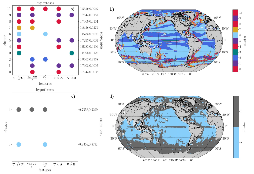
Figure 5: Panels $a)$ and $b)$ show the optimal dominant balances for each cluster and their spatial distributions, respectively, for $K-$means clustering and CHS algorithms. The optimal score $\mathcal{M}(\mathbf{E},\mathbf{H})=0.90$ was found at $K=49$. Panels $c)$ and $d)$ show the optimal dominant balances for each cluster and their spatial distributions, respectively, for HDBSCAN clustering and CHS algorithms. The optimal score $\mathcal{M}(\mathbf{E},\mathbf{H})=0.87$ was found for 50 minimum samples and 200 minimum cluster size. The $K-$means results score higher than the HDBSCAN and they agree with the analysis of Sonnewald et al., [2019].

Sonnewald et al., [2019] calculated the terms in the barotropic vorticity equation for the global ocean, and subsequently used the $K-$means algorithm to partition them into dynamical regimes that were qualitatively interpreted as dominant balances. Since the $K-$means and CHS algorithms and SPCA all implicitly assume that convex, unimodal clusters are present in the data, and the number of equation terms is small, we chose the $K-$means clustering with the CHS algorithm to test the framework shown in Figure 2 on the barotropic vorticity problem of Sonnewald et al., [2019]. They computed a 20-year mean of the Estimating the Circulation and Climate of the Ocean (ECCO) ocean state estimate version 4 release 2 (see Forget et al., [2015], Wunsch and Heimbach, [2013], ECCO Consortium, 2017a , and ECCO Consortium, 2017b ) at 1^∘ resolution to calculate terms of the vertically integrated barotropic vorticity equation, which was grouped and rearranged to be expressed as

$$\overbrace{\nabla\cdot(f\mathbf{U})}^{\begin{subarray}{c}\text{advection of}\\ \text{ planetary vorticity}\end{subarray}}=\hskip 5.69054pt\overbrace{\frac{\nabla p_{b}\times\nabla H}{\rho}}^{\begin{subarray}{c}\text{bottom}\\ \text{pressure torque}\end{subarray}}\hskip 8.53581pt+\overbrace{\frac{\nabla\times\boldsymbol{\tau}}{\rho}}^{\begin{subarray}{c}\text{wind \& bottom}\\ \text{stress curl}\end{subarray}}+\hskip 2.84526pt\overbrace{\nabla\times\mathbf{A}}^{\begin{subarray}{c}\text{nonlinear}\\ \text{torque}\end{subarray}}\hskip 2.84526pt+\hskip 2.84526pt\overbrace{\nabla\times\mathbf{B}}^{\begin{subarray}{c}\text{ diffusive}\\ \text{torque}\end{subarray}}.$$ (19)

In the above, $f$ is the Coriolis parameter, $\mathbf{U}$ is the vertically integrated horizontal velocity, $p_{b}$ is the bottom pressure, $H$ is the depth, $\rho$ is a reference density, $\boldsymbol{\tau}$ represents surface stress, $\nabla$ is applied only to the horizontal coordinates, $\mathbf{A}$ contains nonlinear horizontal momentum fluxes, and $\mathbf{B}$ contains linear horizontal diffusive fluxes.

Figures 5$a)$ and 5$b)$ show the optimal dominant balances for each cluster and their spatial distributions, respectively, for $K-$means clustering and CHS algorithms. The optimal score $\mathcal{M}(\mathbf{E},\mathbf{H})=0.90$ was found at $K=49$. Figures 5$c)$ and 5$d)$ show the optimal dominant balances for each cluster and their spatial distributions, respectively, for HDBSCAN clustering and CHS algorithms. The optimal score $\mathcal{M}(\mathbf{E},\mathbf{H})=0.87$ was found for 50 minimum samples and 200 minimum cluster size. Since the $K-$means results score higher than the HDBSCAN results, $K-$means is the better choice of clustering algorithm for this problem. Figures 5$b)$ and 5$d)$ also show that results that differ only slightly in score can differ in the distribution and labeling of dynamical regimes significantly. This underscores the obligation of the user to choose clustering algorithms that are constructed upon assumptions that are consistent with the notion of a dynamical regime (e.g. dominant mean balances) and that the user must judiciously search parameter space for optimal scores. Crucially, our method allows the user to find the best results (e.g. Figures 5$a)$ and 5$b)$ relative to Figures 5$c)$ and 5$d)$) without relying a priori dynamical knowledge, and the method is applicable to all clustering algorithms and dimensionality reduction algorithms and therefore allows for comparisons of the selected algorithms.

The dominant balances shown in Figures 5$a)$ and 5$b)$ are qualitatively consistent with and quantitatively similar to the analysis of Sonnewald et al., [2019]. In particular, the distribution of the Sverdrup balance (cluster 6, light blue, a balance of planetary advection and wind stress curl) are consistent with the largest magnitude cluster-average terms in Sonnewald et al., [2019] in the same areas, as well as with domain knowledge. The pressure torque $-$ wind stress curl balance (cluster 2, blue) and the nonlinear clusters (purple and red clusters) also agree with Sonnewald et al., [2019].

3.2.3 Reaction-diffusion dynamics in tumor-induced angiogenesis

A common approach to evaluate the dynamical significance of individual equation terms is to calculate numerical solutions with different permutations of terms eliminated. This technique has been used to study tumor angiogenesis (Anderson and Chaplain, [1998], Anderson et al., [2000]), the patterns of growth of cells that facilitate the creation of a pathway for blood to reach a tumor thus enabling tumor growth. We demonstrate that our framework provides a direct evaluation of which terms are dominant without iterating over different eliminated terms.

The continuous tumor-induced angiogenesis model of Anderson and Chaplain, [1998] is composed of conservation laws of three continuous variables: the endothelial-cell density per unit area $n$ (cells that rearrange and migrate from preexisting vasculature to ultimately form new capillaries), the tumor angiogenic factor concentration $c$ (chemicals secreted by the tumor that promote angiogenesis), and the fibronectin concentration $f$ (macromolecules that are secreted by $n$ and stimulate the directional migration of $n$). Endothelial cell migration up the fibronectin concentration gradient is termed haptotaxis (Carter, [1965], Carter, [1967]), while endothelial cell migration up the gradient of tumor angiogenic factor concentration is termed chemotaxis (Sholley et al., [1984]).

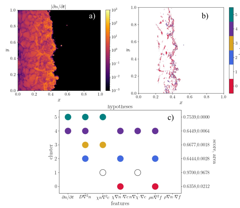
Figure 6: Dominant balance discovery for the nonlinear reaction-diffusion tumor angiogenesis problem of Anderson and Chaplain, [1998], shown at non-dimensional time $t=0.91$. In panel $a)$, the tumor is located at $x,y=1,0.5$, and the endothelial cell growth is propagating in the positive $x$ direction towards the tumor. Panels $b)$ and $c)$ show the regime distributions and dominant balances, respectively, for the optimal results for $K-$means clustering and CHS hypothesis selection.

The non-dimensional, tumor-induced angiogenesis governing equations of Anderson and Chaplain, [1998] are

$$\frac{\partial{n}}{\partial{t}} =\overbrace{D_{a}\nabla^{2}n}^{\text{random motility}}-\hskip 2.84526pt\overbrace{\nabla\cdot(\chi n\nabla c)}^{\text{chemotaxis}}\hskip 2.84526pt-\hskip 2.84526pt\overbrace{\nabla\cdot(\rho_{a}n\nabla f)}^{\text{haptotaxis}},$$ (20)

$$=D_{a}\nabla^{2}n\hskip 2.84526pt-\chi n\nabla^{2}c-\chi\nabla n\cdot\nabla c-n\nabla\chi\cdot\nabla c-\rho_{a}n\nabla^{2}f-\rho_{a}\nabla n\cdot\nabla f,$$ (21)

$$\frac{\partial{f}}{\partial{t}} =\beta_{f}n-\gamma nf,$$ (22)

$$\frac{\partial{c}}{\partial{t}} =-\eta_{c}cn,$$ (23)

where

$$\chi(c)=\frac{\chi_{0}}{1+\alpha_{a}c}.$$ (24)

We numerically solve the same problem as Anderson and Chaplain, [1998], with the exception that 1% amplitude red noise was added to the initial $c$ and $f$ fields in order to provide additional variability for illustrative purposes. Further details of the numerical solutions are provided in the Appendix.

Figure 6 shows the dominant balances of the tumor angiogenesis problem of Anderson and Chaplain, [1998] at non-dimensional time $t=0.91$. The initial conditions are that of Anderson and Chaplain, [1998] with 1% amplitude noise added to the initial angiogenic factor concentration $c$ and fibronectin concentration $f$ fields. $K-$means and CHS algorithms were employed for the partitioning and hypothesis selection tasks of the framework shown in Figure 2. The optimal global magnitude score is $\mathcal{M}(\mathbf{E},\mathbf{H})=0.96$ and it occurs for $K=9$. The dominant balances indicate that the regions of fastest growth/decay of endothelial cell concentration $n$ occur at the front at approximately $x=0.4$, where the $\chi n\nabla^{2}c$ and $\rho_{a}\nabla n\cdot\nabla f$ terms are inactive (cluster 4, purple). The dominant balances also indicate that in regions of weaker growth/decay, the time rate of change endothelial cell concentration is a residual of a balance between $\chi\nabla n\cdot\nabla c\sim\rho_{a}n\nabla^{2}f$, cluster 0 (red). Figure 6 shows that the unsupervised learning framework proposed in this Article provides a more nuanced and direct method for analyzing the effect of individual terms on the growth of a specific variable than running a multitude of simulations with different terms eliminated, as was done by Anderson and Chaplain, [1998].

3.2.4 Spatially-developing turbulent boundary layers

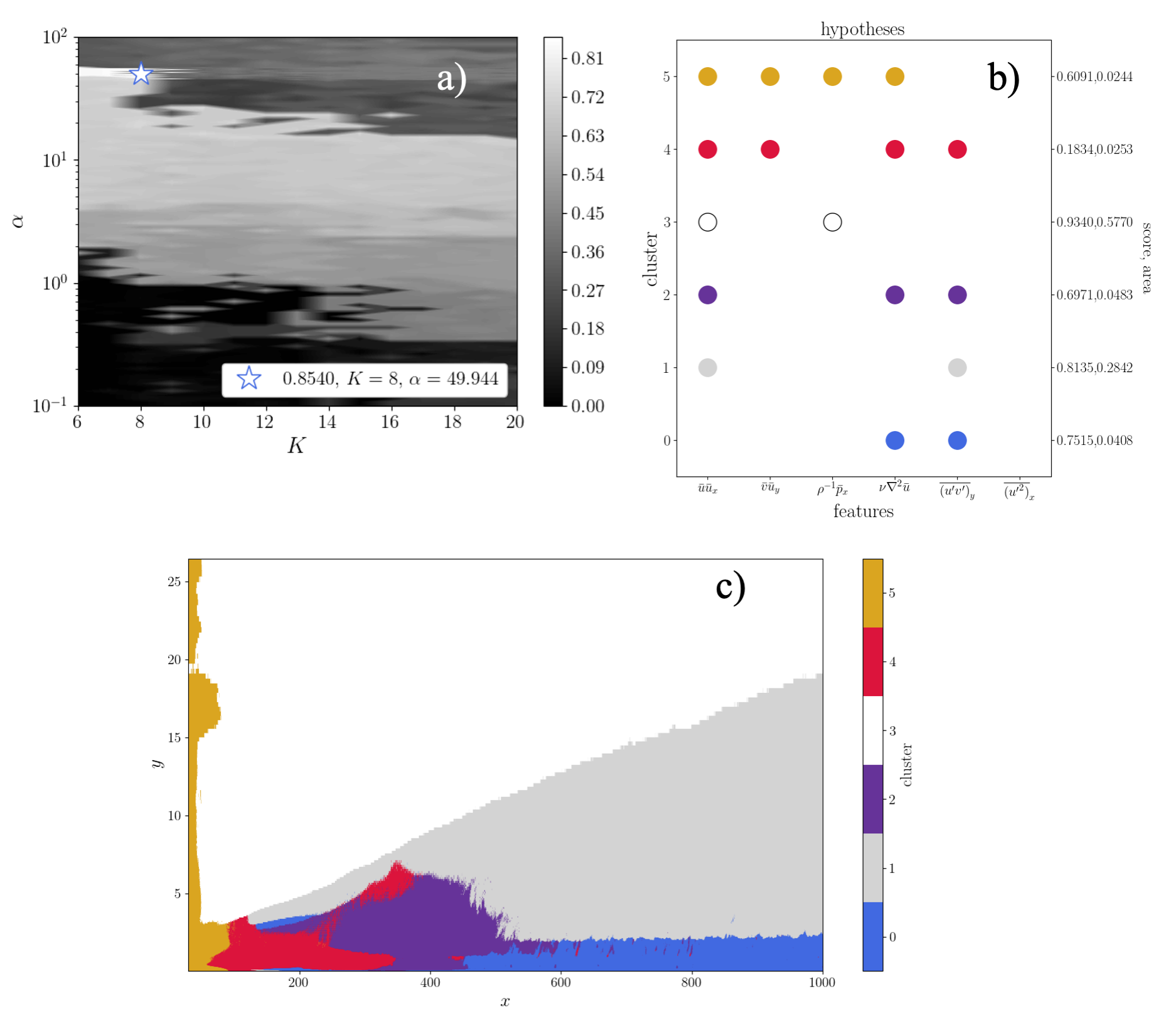
Figure 7: The dominant balances of the spatially-developing turbulent boundary layer. Figure $a)$ shows the global score $\mathcal{M}(\mathbf{E},\mathbf{H})$ as the prescribed number of components for GMM clustering, $K$, and $l_{1}$ LASSO regression coefficient for SPCA, $\alpha$, are varied. The optimal result is $\mathcal{M}(\mathbf{E},\mathbf{H})=0.85$ for $K=8$ and $\alpha=49.94$. Figures $b)$ and $c)$ show that the optimal is consistent with the results shown in Callaham et al., [2021] and with domain knowledge, where the blue cluster is the viscous sublayer, the grey cluster is the region of the so-called law of the wall, and the white cluster is the free stream flow.

In this section we apply the framework in Figure 2 to one of the dynamical regime problems that Callaham et al., [2021] solved by using Gaussian Mixture Model (GMM) clustering and SPCA: the turbulent boundary layer (TBL) that develops as a high speed flow blows over a flat plate. We use the same data set as Callaham et al., [2021]: the turbulent boundary layer direct numerical simulation data available in the Johns Hopkins University turbulence database (Zaki, [2013]). The equation that governs the velocity in the direction of the mean flow, $u$, also known as the boundary layer equation (Tennekes et al., [1972]), is

$$\overbrace{\overline{u}\frac{\partial\overline{u}}{\partial\hat{x}}+{\overline{v}\frac{\partial\overline{u}}{\partial\hat{y}}}}^{\begin{subarray}{c}\text{mean}\\ \text{momentum flux}\\ \text{divergence}\end{subarray}}\hskip 5.69054pt=\overbrace{-\frac{1}{\rho}\frac{\partial\overline{p}}{\partial\hat{x}}}^{\begin{subarray}{c}\text{mean}\\ \text{pressure gradient}\end{subarray}}+\overbrace{\nu\nabla^{2}\overline{u}}^{\begin{subarray}{c}\text{mean}\\ \text{momentum}\\ \text{diffusion}\end{subarray}}-\hskip 2.84526pt\overbrace{\frac{\partial\overline{u^{\prime}v^{\prime}}}{\partial\hat{y}}-\frac{\partial\overline{u^{\prime 2}}}{\partial\hat{x}}}^{\begin{subarray}{c}\text{turbulent}\\ \text{momentum flux}\\ \text{divergence}\end{subarray}},$$ (25)

where the velocity and pressure fields ($u,v,p$) have been decomposed into mean and fluctuating components denoted by overbars and primes, respectively: the $x$ direction points in the downwind direction, and the $y$ direction points in the direction normal to the surface. The averaging operator represents averaging over the spanwise direction as well as averaging over time, and the diffusion operator is defined as $\nabla^{2}=\partial^{2}/\partial\hat{x}^{2}+\partial^{2}/\partial\hat{y}^{2}$. $\rho$ and $\nu$ are constants that represent the fluid density and kinematic viscosity, respectively.

The optimal results shown in Figure 7 are qualitatively consistent with and quantitatively similar to the results of Callaham et al., [2021], with the notable difference that here the optimal clustering and dimensionality reduction parameters are defined by the objective function instead of by the user’s knowledge of the algorithms. Clusters 0, 1, and 3 (blue, grey, and white, respectively) are consistent with established domain knowledge of viscous sublayers, the law of the wall, and free stream flow, respectively (Schetz and Bowersox, [2011]) but have been identified by a completely objective technique for the first time. Slight differences between the results shown in Figure 7 and Callaham et al., [2021] arise from standardization of the equation data prior to clustering and from normalization of the cluster data prior to dimensionality reduction.

4 Time complexity

While our framework (Figure 2) and proposed objective function (Equation 13) yield robust solutions to Equation 1 for data sets with obvious dynamical regimes (e.g. Section 3.2.1), the time complexity of the framework depends upon the chosen clustering algorithm and hypothesis selection algorithms. A comprehensive analysis of all possible algorithm choices is beyond the scope of this Article, though we can infer general properties of the complexity of the framework. The search over hyperparameters may very well be NP-hard; indeed, the search over hyperparameter $K$, the prescribed number of clusters for $K-$means, to minimize the sum of the square of the Euclidean distance of each data point to its nearest center is NP-hard even for just two features, $D=2$ (Mahajan et al., [2012]). Furthermore, a näive search over a potentially infinite number of hyperparameters is obviously unfeasible, therefore practical implementation of the framework depends upon the familiarity of the user with the chosen algorithms and the statistical properties of the given data set.

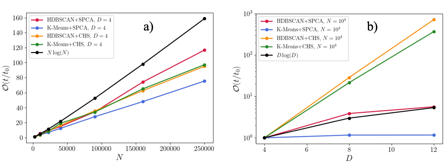
Figure 8: Time complexities of the framework shown in Figure 2 for different clustering and hypothesis selection algorithms as a function of the size of the input data set $N$ ($a$) and as a function of the size of the number of equation terms $D$ ($b$) when computed using the synthetic data described in Equations 16-18 and Table 1. The optimal dominant balances, their distributions, and global magnitude score for all complexity examples are identical.

The time complexity of different clustering and hypothesis selection algorithm choices applied to the synthetic data problem (Figure 4) is shown in Figure 8. Each data point in Figures 8a) and 8b) represents the average wall clock time for one pass through the framework in Figure 2, i.e. for a single set of hyperparameters. Figure 8$a)$ shows that combining SPCA (Zou et al., [2006] with either $K-$means by Expectation-Maximization (Bishop, [2006]) or HDBSCAN (Campello et al., [2015]), which are parametric and non-parametric clustering algorithms, respectively, results in computational times that scale polynomially in the data set sample size $N$. In Figures 8$a)$ and 8$b)$, the computational time spent on one cycle for a given $N$ or $D$, by each algorithmic choice, is normalized by $t_{0}$, the computational time taken for the smallest $N$ or $D$, respectively.

As expected by its construction, Figure 8$b)$ shows that the CHS is prohibitively complex as the number of equation terms increases because its complexity scales with $\mathcal{O}(2^{D})$. However, the advantage of the CHS algorithm is that it has no hyperparameters; therefore, for equations with only a handful of terms, between 3 to 5 terms, we recommend using CHS over SPCA, which has a LASSO regression coefficient that must be optimized in addition to clustering algorithm parameters. For equations with more terms, we recommend SPCA, but there are many other possible choices, viz. Van Der Maaten et al., [2009].

In summary, our framework yields robust solutions to Equation 1 for data sets with obvious dynamical regimes (e.g. Section 3.2.1), but efficient computation requires the user to consider the size of the data set $N$ and the number of equation terms $D$ when selecting clustering and hypothesis selection algorithms.

5 Conclusions

We have formalized the problem of identifying dynamical regimes as an optimization problem in which data, consisting of the terms in an equation that describes the complete dynamics of a physical process, is partitioned into clusters of unique, reduced sets of terms that are dominant in the equation. The optimization is achieved by maximizing an objective function that we have defined such that it favors large magnitude differences between selected and neglected terms, and penalizes large magnitude spread within the selected terms. Our formulation of the problem and our definition of the objective function are independent of the method chosen to label each observation as a dominant balance and, together, they transform a form of analysis of data of dynamical systems that was previously an ad hoc, heuristic notion, into an objective method for the identification of non-asymptotic dynamical regimes.

We demonstrated how this formulation of the problem can be applied to an unsupervised learning framework, in which equation data is partitioned by clustering algorithms (Sonnewald et al., [2019], Callaham et al., [2021]), labeled by hypotheses generated by a dimensionality reduction algorithm (Callaham et al., [2021]), and finally optimized over algorithm parameters using our objective function. This was demonstrated on synthetic data with obvious dominant terms separated by a sharp regime boundary as well as with three examples drawn from climate dynamics, cancer modeling, and aerodynamics. We demonstrate how the dynamical regime problem can be solved by an unsupervised learning framework for fixed algorithm parameters, and we note that a näive search of possible infinite algorithm parameter space for a global optimum is computationally unfeasible. We have effectively exchanged prerequisite domain knowledge with a familiarity with and skill at using clustering and dimensionality reduction algorithms, thus opening the door to rapid dynamical regime discovery within large data sets.

6 Acknowledgements

This work was performed under the auspices of DOE. Financial support comes partly from Los Alamos National Laboratory (LANL), Laboratory Directed Research and Development (LDRD) project ”Machine Learning for Turbulence,” 20180059DR. LANL, an affirmative action/equal opportunity employer, is managed by Triad National Security, LLC, for the National Nuclear Security Administration of the U.S. Department of Energy under contract 89233218CNA000001. Computational resources were provided by the Institutional Computing (IC) program at LANL.

MS acknowledges funding from Cooperative Institute for Modeling the Earth System, Princeton University, under Award NA18OAR4320123 from the National Oceanic and Atmospheric Administration, U.S. Department of Commerce. The statements, findings, conclusions, and recommendations are those of the authors and do not necessarily reflect the views of Princeton University, the National Oceanic and Atmospheric Administration, or the U.S. Department of Commerce.

7 Appendices

7.1 Parameter ranges for time complexity calculations

The average wall time elapsed for the framework computations over hyperparameter ranges are shown in Figure 8. The hyperparameter ranges were specfied as follows. For $K-$means clustering the number of prescribed clusters $K$ was specified as $K=\{2,...,10\}$ and the other hyperparameters were the default choices as provided by SciKit Learn (Pedregosa et al., [2011]). For HDBSCAN clustering the prescribed minimum number of samples for a cluster was specified as 100 samples, and the minimum cluster size was varying from 2000 samples to 3000 samples. For hypothesis selection by SPCA, the LASSO regression coefficient was varied between $10^{-2}$ and $10^{2}$.

7.2 Tumor-induced angiogenesis simulation

A second-order accurate finite difference code was used to calculate each term in the expanded form of the endothelial cell density equation, such that $\mathbf{E}$ is composed of observations of the terms in Equation (21). We employ the same boundary conditions, initial conditions, and constant coefficients ($D_{a}$, $\alpha_{a}$, $\chi_{0}$, $\rho_{a}$, $\beta_{f}$, $\gamma$, and $\eta_{c}$) as Anderson and Chaplain, [1998] at double the resolution. Second-order finite differences were employed for spatial derivatives and 4th-order adaptive Runge-Kutta was employed for the temporal evolution. No-flux boundary conditions were applied to all four boundaries of the square domain:

$$\mathbf{n}\cdot(D_{a}\nabla n-\chi(c)n\nabla c-\rho_{a}n\nabla f)=0,$$ (26)

where $\mathbf{n}$ is the unit normal vector to the boundaries. The initial conditions, for a circular tumor some distance from three clusters of endothelial cells, are:

$$c(x,y,0)=\begin{cases}1,\hskip 22.76219pt\qquad 0\leq r\leq 0.1\\ \frac{(\nu-r)^{2}}{\nu-r_{0}},\qquad 0.1<r\leq 1\end{cases},$$ (27)

where $r=\sqrt{(x-x_{0})^{2}+(y-y_{0})^{2}}$.

$$f(x,y,0)=k\mathrm{e}^{-\frac{x^{2}}{\epsilon_{1}}},$$ (28)

$$n(x,y,0)=\mathrm{e}^{-\frac{x^{2}}{\epsilon_{2}}}\sin^{2}(6\pi y),$$ (29)

where $\nu=(\sqrt{5}-0.1)/(\sqrt{5}-1)$, $r_{0}=0.1$, $x_{0}=1$, $y_{0}=1/2$, $k=0.75$, $\epsilon_{1}=0.45$, $\epsilon_{2}=0.001$. The constant coefficients were specified as $D_{a}=0.00035$, $\alpha_{a}=0.6$, $\chi_{0}=0.38$, $\rho_{a}=0.34$, $\beta_{f}=0.05$, $\gamma=0.1$, and $\eta_{c}=0.1$.

References

- Anderson et al., [2000] Anderson, A. R., Chaplain, M. A., Newman, E. L., Steele, R. J., and Thompson, A. M. (2000). Mathematical modelling of tumour invasion and metastasis. Computational and mathematical methods in medicine, 2(2):129–154.
- Anderson and Chaplain, [1998] Anderson, A. R. and Chaplain, M. A. J. (1998). Continuous and discrete mathematical models of tumor-induced angiogenesis. Bulletin of mathematical biology, 60(5):857–899.
- Bishop, [2006] Bishop, C. M. (2006). Pattern recognition and machine learning. springer.
- Callaham et al., [2021] Callaham, J. L., Koch, J. V., Brunton, B. W., Kutz, J. N., and Brunton, S. L. (2021). Learning dominant physical processes with data-driven balance models. Nature communications, 12(1):1–10.
- Campello et al., [2015] Campello, R. J., Moulavi, D., Zimek, A., and Sander, J. (2015). Hierarchical density estimates for data clustering, visualization, and outlier detection. ACM Transactions on Knowledge Discovery from Data (TKDD), 10(1):1–51.
- Carter, [1965] Carter, S. B. (1965). Principles of cell motility: the direction of cell movement and cancer invasion. Nature, 208(5016):1183–1187.
- Carter, [1967] Carter, S. B. (1967). Haptotaxis and the mechanism of cell motility. Nature, 213(5073):256–260.
- Cormen et al., [2009] Cormen, T. H., Leiserson, C. E., Rivest, R. L., and Stein, C. (2009). Introduction to algorithms. MIT press.
- Currie, [2016] Currie, I. G. (2016). Fundamental mechanics of fluids. CRC press.
- d’Alembert, [1752] d’Alembert, J. L. R. (1752). Essai d’une nouvelle théorie de la résistance des fluides. David l’aîné.
- Dy and Brodley, [2004] Dy, J. G. and Brodley, C. E. (2004). Feature selection for unsupervised learning. Journal of machine learning research, 5(Aug):845–889.
- [12] ECCO Consortium (2017a). A twenty-year dynamical oceanic climatology: 1994-2013. part 1: Active scalar fields: Temperature, salinity, dynamic topography, mixed-layer depth, bottom pressure.
- [13] ECCO Consortium (2017b). A twenty-year dynamical oceanic climatology: 1994-2013. part 2: Velocities, property transports, meteorological variables, mixing coefficients.
- Estivill-Castro, [2002] Estivill-Castro, V. (2002). Why so many clustering algorithms: a position paper. ACM SIGKDD explorations newsletter, 4(1):65–75.
- Forget et al., [2015] Forget, G., Campin, J.-M., Heimbach, P., Hill, C. N., Ponte, R. M., and Wunsch, C. (2015). Ecco version 4: An integrated framework for non-linear inverse modeling and global ocean state estimation.
- Hartigan, [1975] Hartigan, J. A. (1975). Clustering algorithms. John Wiley & Sons, Inc.
- Kohavi and John, [1997] Kohavi, R. and John, G. H. (1997). Wrappers for feature subset selection. Artificial intelligence, 97(1-2):273–324.
- MacQueen et al., [1967] MacQueen, J. et al. (1967). Some methods for classification and analysis of multivariate observations. In Proceedings of the fifth Berkeley symposium on mathematical statistics and probability, volume 1, pages 281–297. Oakland, CA, USA.
- Mahajan et al., [2012] Mahajan, M., Nimbhorkar, P., and Varadarajan, K. (2012). The planar k-means problem is np-hard. Theoretical Computer Science, 442:13–21.
- Munk, [1950] Munk, W. H. (1950). On the wind-driven ocean circulation. Journal of Atmospheric Sciences, 7(2):80–93.
- Munkres, [2000] Munkres, J. R. (2000). Topology: international edition. Pearson Prentice Hall.
- Pearson and Sekar, [1936] Pearson, E. S. and Sekar, C. C. (1936). The efficiency of statistical tools and a criterion for the rejection of outlying observations. Biometrika, 28(3/4):308–320.
- Pedregosa et al., [2011] Pedregosa, F., Varoquaux, G., Gramfort, A., Michel, V., Thirion, B., Grisel, O., Blondel, M., Prettenhofer, P., Weiss, R., Dubourg, V., Vanderplas, J., Passos, A., Cournapeau, D., Brucher, M., Perrot, M., and Duchesnay, E. (2011). Scikit-learn: Machine learning in Python. Journal of Machine Learning Research, 12:2825–2830.
- Peixoto and Oort, [1992] Peixoto, J. P. and Oort, A. H. (1992). Physics of climate.
- Poincaré, [1905] Poincaré, H. (1905). Science and hypothesis. Science Press.
- Prandtl, [1904] Prandtl, L. (1904). Über flussigkeitsbewegung bei sehr kleiner reibung. Verhandl. III, Internat. Math.-Kong., Heidelberg, Teubner, Leipzig, 1904, pages 484–491.
- Rousseeuw, [1987] Rousseeuw, P. J. (1987). Silhouettes: a graphical aid to the interpretation and validation of cluster analysis. Journal of computational and applied mathematics, 20:53–65.
- Rudin, [2019] Rudin, C. (2019). Stop explaining black box machine learning models for high stakes decisions and use interpretable models instead. Nature Machine Intelligence, 1(5):206–215.
- Schetz and Bowersox, [2011] Schetz, J. A. and Bowersox, R. D. (2011). Boundary layer analysis. American Institute of Aeronautics and Astronautics.
- Sholley et al., [1984] Sholley, M., Ferguson, G., Seibel, H., Montour, J., and Wilson, J. (1984). Mechanisms of neovascularization. vascular sprouting can occur without proliferation of endothelial cells. Laboratory investigation; a journal of technical methods and pathology, 51(6):624–634.
- Smagorinsky, [1969] Smagorinsky, J. (1969). Problems and promises of deterministic extended range forecasting. Bulletin of the American Meteorological Society, 50(5):286–312.
- Sonnewald et al., [2019] Sonnewald, M., Wunsch, C., and Heimbach, P. (2019). Unsupervised learning reveals geography of global ocean dynamical regions. Earth and Space Science, 6(5):784–794.
- Strogatz, [2018] Strogatz, S. H. (2018). Nonlinear dynamics and chaos with student solutions manual: With applications to physics, biology, chemistry, and engineering. CRC press.
- Tennekes et al., [1972] Tennekes, H., Lumley, J. L., Lumley, J. L., et al. (1972). A first course in turbulence. MIT press.
- Tibshirani, [1996] Tibshirani, R. (1996). Regression shrinkage and selection via the lasso. Journal of the Royal Statistical Society: Series B (Methodological), 58(1):267–288.
- Vallis, [2017] Vallis, G. K. (2017). Atmospheric and oceanic fluid dynamics. Cambridge University Press.
- Van Der Maaten et al., [2009] Van Der Maaten, L., Postma, E., and Van den Herik, J. (2009). Dimensionality reduction: a comparative. J Mach Learn Res, 10(66-71):13.
- Wang et al., [2018] Wang, J., Oh, J., Wang, H., and Wiens, J. (2018). Learning credible models. In Proceedings of the 24th ACM SIGKDD International Conference on Knowledge Discovery & Data Mining, pages 2417–2426.
- Wunsch and Heimbach, [2013] Wunsch, C. and Heimbach, P. (2013). Dynamically and kinematically consistent global ocean circulation and ice state estimates. In International Geophysics, volume 103, pages 553–579. Elsevier.
- Zaki, [2013] Zaki, T. A. (2013). From streaks to spots and on to turbulence: exploring the dynamics of boundary layer transition. Flow, turbulence and combustion, 91(3):451–473.
- Zohuri, [2017] Zohuri, B. (2017). Dimensional analysis beyond the Pi theorem. Springer.
- Zou et al., [2006] Zou, H., Hastie, T., and Tibshirani, R. (2006). Sparse principal component analysis. Journal of computational and graphical statistics, 15(2):265–286.